


Median Housing Price Prediction Model for D. M. Pan National Real Estate Company 1
Report: Housing Price Prediction Model forD. M. Pan National Real Estate Company
Max Harrop
Southern New Hampshire University

Median Housing Price Model for D. M. Pan National Real Estate Company 2
Introduction
We are trying to predict if the median housing listing price with the median square
footage, this is by using different graphs, tables, linear regression, and samples to make an
analysis. By using liner aggression, we can expect there is some type of correlation between the
two variables. It is most appropriate when we are trying to predict the strength and the trend of a
set data. This can be shown by determining how much the square footage of a house can have an
impact on its listing price. The first variable or the (predictor variable) is going to be used to
predict and the other variable or the (response variable) is what are trying to predict. In this case
the median square footage of the house is the predictor variable, and the median listing price is
the response variable. If we want to detrmine the median listing price we need to use the median
square footage.
Data Collection
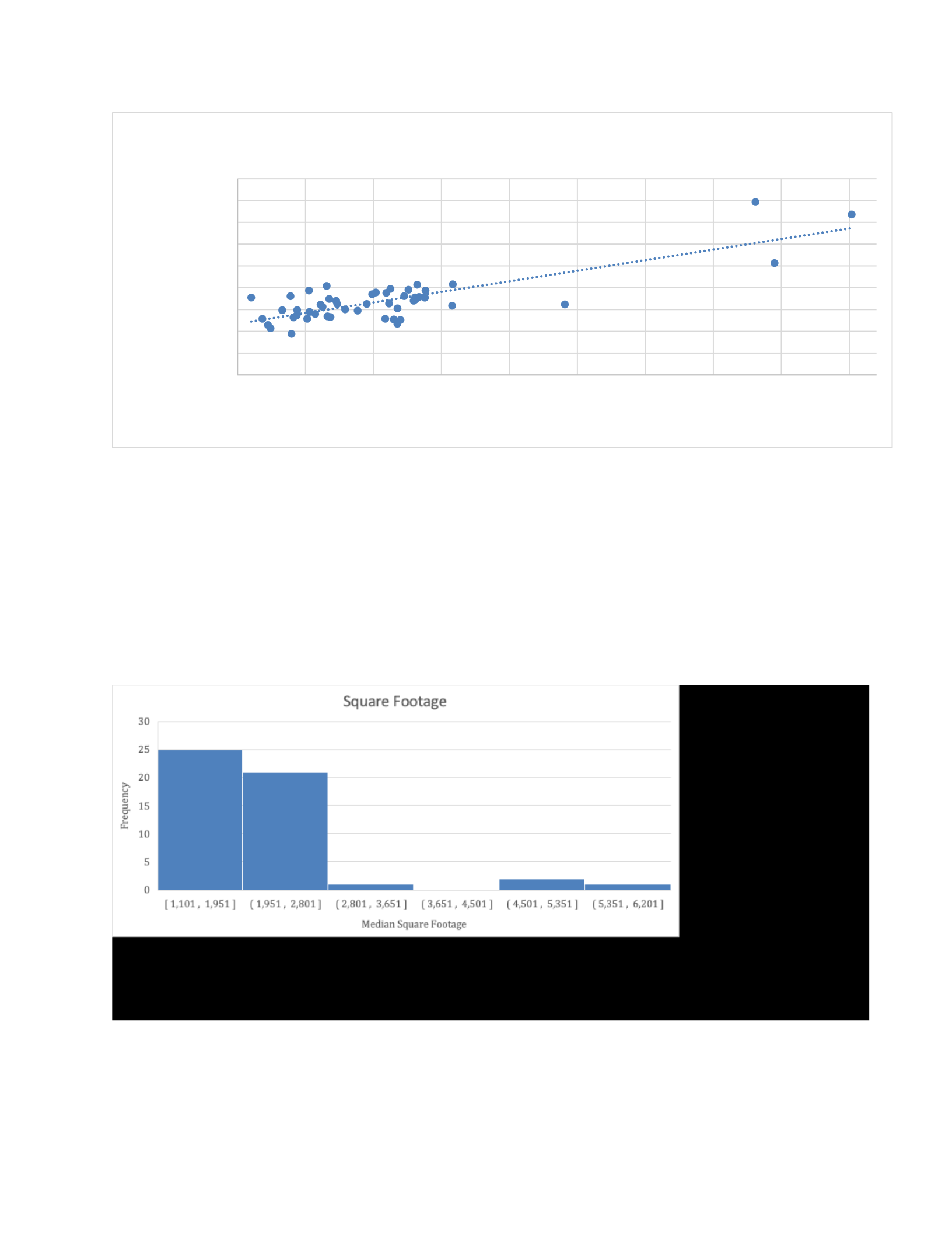
I was able to obtain sample data by using the excel equation =RAND(). I started by
making a new column called random, then put the equation in and it made a bunch of random
numbers. Next, I selected all my columns and sells, then used the sort feature to randomly sort all
my data. I then selected the first 50 counties on the data sheet, X= the median square feet and Y=
the median listing price.
Median Housing Price Model for D. M. Pan National Real Estate Company 3
1,000 1,500 2,000 2,500 3,000 3,500 4,000 4,500 5,000 5,500
-
100,000
200,000
300,000
400,000
500,000
600,000
700,000
800,000
900,000
Square Footage vs. Listing Price
Square Footage
Listing Price
Data Analysis
Before we can create a linear regression model there are assumptions that must be
met. This is so the data, or the true relationship is linear, errors can have equal variance
that is around the line, and errors can be normally distributed. The predictor variable is
median square footage, and the response variable is the median listing price.
Median Housing Price Model for D. M. Pan National Real Estate Company 4
Square Footage Listing Price
Mean 2,082 $340,353
Median 1,971 $325,300
Standard Dev 891,906.00 $106807.33
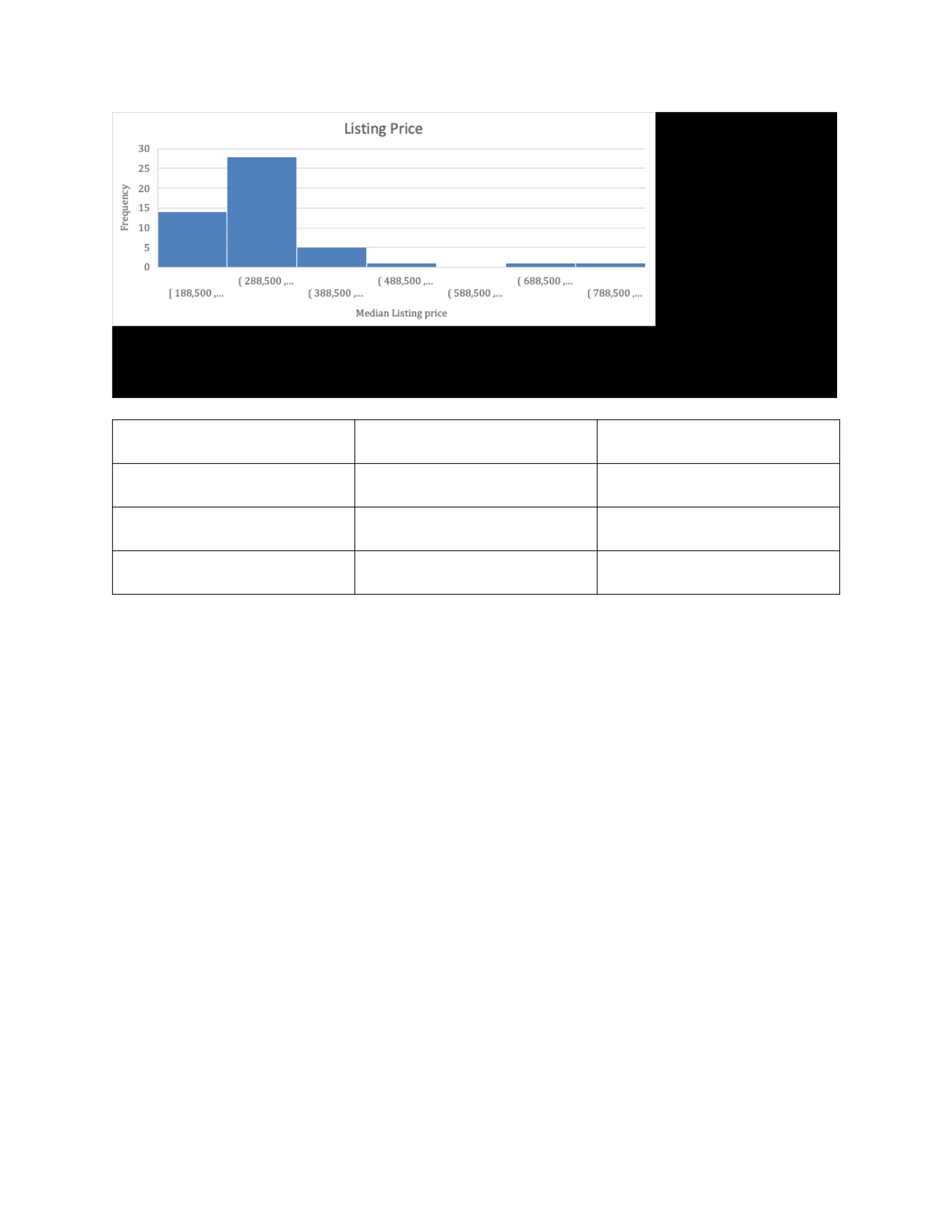
In the first histogram it shows the median square footage of the houses. We can see that
there is a gap in the histogram where the square footage is 3,651-4,501 there are no houses in the
fifty samples that are in that square footage, this would be the biggest outlier in the graph.
Another outlier is that we can see that there are very little houses that are above 2,801 square
feet. All the way to the left it shows us that there are 25 houses that are 1,101-1951 square feet.
This means that most of the houses in this sample are between that square footage. In the second
histogram it shows us that most of the houses about 28 of them are priced from $288,500-
$388,500. There is one big outlier in this histogram as well and that is that there is a gap for
houses that would be priced $588,500-$688,500. Another outlier is that most of the houses are
between $188,500-$388,500)
Median Housing Price Model for D. M. Pan National Real Estate Company 5
When we look at the random sample of fifty counties versus the national average, we see
that the national median square footage is 1,881 and in our sample it’s 1,971. This means that the
median square footage in my sample is 90 square feet more than the national average. When we
look at the fifty counties and the national average, we see that the national median listing price is
$342,365 and the median listing price in my random sample is $325,300. That is about $17,062
difference in the national average and the sample.
1,000 1,500 2,000 2,500 3,000 3,500 4,000 4,500 5,000 5,500
-
100,000
200,000
300,000
400,000
500,000
600,000
700,000
800,000
900,000
f(x) = 97.0081048632925 x + 138394.706809306
R² = 0.656223984620144
Square Footage vs. Listing Price
Square Footage
Listing Price
Develop Regression Model
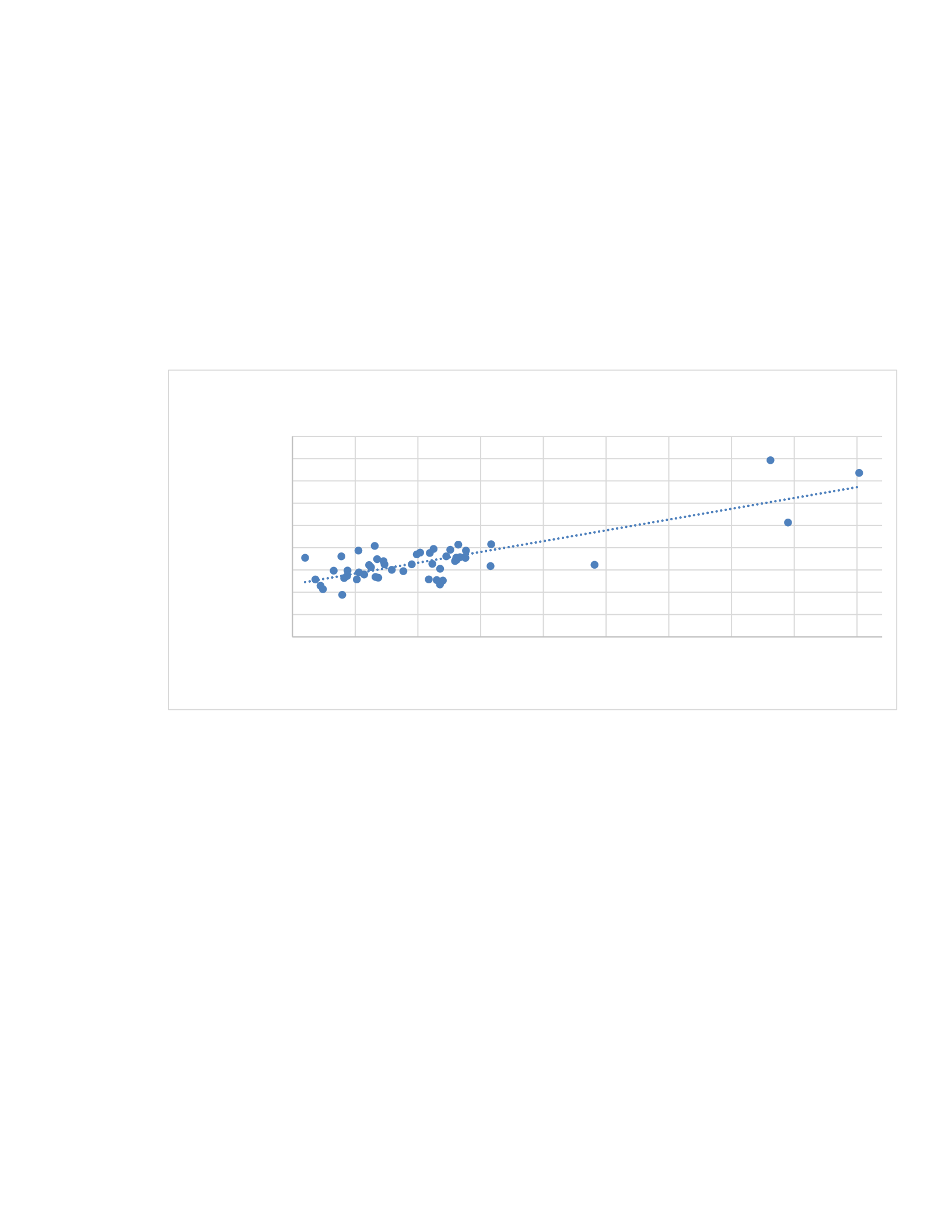
The regression model can be developed for the data, this is because based on the scatterplot
above we can see that the data has a positive correlation, and this is a true linear relationship. We
see this trendline, and it shows us that when the square footage goes up so does the listing price
of the houses. While we can see that there is moderate correlation in the data and it’s a positive
correlation. There are a few dots that we can see that are a bit off the line and if it where up to me
those would be removed. The value of r is 0.81 and these supports a positive correlation, this is
because when one of our variables increases, the other does based on that increase.

Median Housing Price Model for D. M. Pan National Real Estate Company 6
Determine the Line of Best Fit
Regression Equation y=97.008x+138395
What we can see from this equation is that the median listing price or (x) is what a home
should be listed at when (x) is replaced with the square footage of the house. For example, if (x)
was 0 then the listing price would be $138,395, that would mean that value is positive. For every
increase of square footage, the listing price would go up 97.008. R-squared tells us the
percentage of sample data that’s close to the line. That doesn’t tell us the in the future how likely
we are to get on that line because we don’t know what we are going to get in the future. If the
house was 1,500sqft then the listing price would be $283,907. We were able to find this because
we used the regression equation y=97.008(1500) +138396.
Conclusions
When using the data above, I can see that it is suitable to determine what the median
listing price of a house should be based on the square footage of that house. This is what I
thought was going to be found in the data and sample that I used. It was further confirmed that
once built into the histograms and scatterplots that my data shows what we were able to
determine. I think it would be interesting to see this data from a sample of fifty random counites
against another sample to see how different they are. These fifty counites are all from different
regions and states, this is just a national average based on these fifty counties.

