



MATH 402 - LINEAR REGRESSION -
Least Squares Estimation
Question Bank - Set 9
Liberty University
Question 1
Question
Let Ybe a random variable representing the sales revenue (in thousands of dol-
lars) of a company, and let Xbe a random variable representing the advertising
expenditure (in thousands of dollars) of the same company. The following data
was collected for 6 months:
Month 1 2 3 4 5 6
X2 4 6 5 8 7
Y3 5 7 6 9 8
Determine the least squares estimate of the regression line that predicts sales
revenue based on advertising expenditure.
Solution
Step 1: Let’s first calculate the mean values of Xand Y:
¯
X=1
6
6
∑
i=1
Xi=2+4+6+5+8+7
6= 5
¯
Y=1
6
6
∑
i=1
Yi=3+5+7+6+9+8
6= 6.33

Step 2: Next, we calculate the deviations from the means for each month:
dX=X−¯
X= (2 −5) (4 −5) (6 −5)
(5 −5) (8 −5) (7 −5)
=−3−1
1 0 3
dY=Y−¯
Y= (3 −6.33) (5 −6.33) (7 −6.33)
(6 −6.33) (9 −6.33) (8 −6.33)
=−3.33 −1.33
0.67 −0.33 2.67
Step 3: Now, we calculate the sum of the products of the deviations:
∑dXdY= (−3)(−3.33) + (−1)(−1.33) + (1)(0.67) + (0)(−0.33) + (3)(2.67)
∑dXdY= 9.99 + 1.33 + 0.67+0+8.01 = 19
Step 4: Calculate the sum of the squares of the deviations of X:
∑d2
X= (−3)2+ (−1)2+ (1)2+ (0)2+ (3)2= 3 + 1 + 1 + 0 + 9 = 14
Step 5: The least squares estimates of the coefficients are:
ˆ
β1=∑dXdY
∑d2
X
=19
14 ≈1.36
ˆ
β0=¯
Y−ˆ
β1¯
X= 6.33 −1.36 ×5≈ −0.33
Therefore, the least squares estimate of the regression line is ˆ
Y≈ −0.33 +
1.36X.
Question 3
Question
Suppose we have a dataset with the following pairs of data: (x1, y1) = (2,5),
(x2, y2) = (4,9),(x3, y3) = (6,11), and (x4, y4) = (8,14). We want to model
the relationship between xand yusing a linear regression model of the form
ˆy=β0+β1x. Find the regression coefficients β0and β1using the method of
least squares estimation.
Solution
Step 1: Compute the means of xand y. The means are given by:
¯x=1
4(2 + 4 + 6 + 8) = 5
2

¯y=1
4(5 + 9 + 11 + 14) = 9.75
Step 2: Compute the sample variances of xand y. The sample variances are
given by:
s2
x=1
3
4
∑
i=1
(xi−¯x)2=1
3[(2 −5)2+ (4 −5)2+ (6 −5)2+ (8 −5)2] = 6.67
s2
y=1
3
4
∑
i=1
(yi−¯y)2=1
3[(5−9.75)2+(9−9.75)2+(11−9.75)2+(14−9.75)2]≈13.46
Step 3: Compute the sample covariance of xand y. The sample covariance
is given by:
sxy =1
3
4
∑
i=1
(xi−¯x)(yi−¯y) = 1
3[(2−5)(5−9.75)+(4−5)(9−9.75)+(6−5)(11−9.75)+(8−5)(14−9.75)] ≈9.25
Step 4: Compute the regression coefficients β0and β1. The slope β1is
calculated as:
β1=sxy
s2
x
≈9.25
6.67 ≈1.39
The intercept β0is then found from:
β0= ¯y−β1¯x= 9.75 −1.39 ×5≈2.90
Therefore, the estimated regression model is ˆy= 2.90 + 1.39x.
Question 4
Question
Let X=
1 3
1 4
1 5
1 6
and Y=
2
4
6
8
. Find the least squares estimate of the vector
β=(β0
β1)in the linear regression model Y=Xβ +εwhere ε∼N(0, σ2I).
Solution
Step 1: The least squares estimate of βis given by ˆ
β= (XTX)−1XTY.
Step 2: First, we calculate XTX:
XTX=(1111
3456)
1 3
1 4
1 5
1 6
=(4 18
18 86)
3

Step 3: Next, we calculate XTY:
XTY=(1 1 1 1
3 4 5 6)
2
4
6
8
=(20
80)
Step 4: Now, we find (XTX)−1:
(XTX)−1=(4 18
18 86)−1
=1
4·86 −18 ·18 (86 −18
−18 4 )
=1
308 (86 −18
−18 4 )
Step 5: Finally, we calculate ˆ
β:
ˆ
β=1
308 (86 −18
−18 4 )(20
80)=1
308 (1592
232 )=(5.16
0.75)
Therefore, the least squares estimate of βis ˆ
β=(5.16
0.75).
Question 5
Question
Let Y1, Y2, . . . , Ynbe a random sample from a normal population with mean µ
and variance σ2. Consider the simple linear regression model
Yi=β0+β1xi+εi
where εi’s are independent N(0, σ2)random variables.
Show that the least squares estimators ˆ
β0and ˆ
β1are unbiased for β0and
β1, respectively.
Solution
Step 1: To show that ˆ
β0is an unbiased estimator for β0, we need to find E(ˆ
β0)
and show that it equals β0.
E(ˆ
β0) = E(¯
Y−ˆ
β1¯x)=E(1
n
n
∑
i=1
Yi−ˆ
β1
1
n
n
∑
i=1
xi)
4

Step 2: Since ¯
Y=¯
β0+¯
β1¯x, we can expand the expression.
E(ˆ
β0) = 1
n
n
∑
i=1
E(Yi)−ˆ
β1
1
n
n
∑
i=1
E(xi)
Step 3: Since Yifollows a normal distribution with mean µ,E(Yi) = µ. Also,
E(xi) = E(x) = µx.
E(ˆ
β0) = 1
n
n
∑
i=1
µ−ˆ
β1
1
n
n
∑
i=1
µx
Step 4: Simplifying the expression further, we get
E(ˆ
β0) = µ−ˆ
β1µx
Step 5: Since µ=β0and µxis the true mean of x, we have E(ˆ
β0) = β0.
This shows that ˆ
β0is an unbiased estimator for β0.
Step 6: Similarly, we can show that ˆ
β1is an unbiased estimator for β1by
finding E(ˆ
β1)and showing that it equals β1.
Therefore, both least squares estimators ˆ
β0and ˆ
β1are unbiased for β0and
β1, respectively.
Question 6
Question
Let X=
1 1
1 2
1 3
1 4
be the design matrix for a linear regression problem with
response vector Y=
2
4
5
7
. Find the least squares estimate of the regression
coefficients.
Solution
Step 1: The least squares estimate of the regression coefficients ˆ
βis given by
the formula: ˆ
β= (XTX)−1XTY
Step 2: First, calculate XTXby multiplying XTand X:
XT=(1 1 1 1
1 2 3 4)
5

XTX=(1111
1234)
1 1
1 2
1 3
1 4
=(4 10
10 30)
Step 3: Next, calculate XTYby multiplying XTand Y:
Y=
2
4
5
7
XTY=(1 1 1 1
1 2 3 4)
2
4
5
7
=(18
46)
Step 4: Now, calculate (XTX)−1by finding the inverse of XTX:
(XTX)−1=(4 10
10 30)−1
=(3
20 −1
10
−1
10
2
5)
Step 5: Finally, calculate the least squares estimate of the regression coeffi-
cients ˆ
β:
ˆ
β= (XTX)−1XTY=(3
20 −1
10
−1
10
2
5)(18
46)=(2
1)
Therefore, the least squares estimate of the regression coefficients is ˆ
β=
(2
1).
Question 7
Question
Let Yi=a+bXi+eibe a simple linear regression model where Yirepresents
the response variable, Xirepresents the predictor variable, arepresents the
intercept, brepresents the slope, and eirepresents the error term for the ith
observation. Consider the following data points:
X Y
1 4
2 7
3 8
4 11
Determine the least squares estimation for the coefficients aand bin the model.
6

Solution
Step 1: Calculate the means of Xand Y. The means are given by:
¯
X=1+2+3+4
4= 2.5
¯
Y=4+7+8+11
4= 7.5
Step 2: Calculate the sum of products and sum of squares. We need to
calculate: n
∑
i=1
XiYi,
n
∑
i=1
X2
i,and
n
∑
i=1
Y2
i
Substitute the given values:
∑XiYi= 1 ∗4+2∗7+3∗8+4∗11 = 4 + 14 + 24 + 44 = 86
∑X2
i= 12+ 22+ 32+ 42= 1 + 4 + 9 + 16 = 30
∑Y2
i= 42+ 72+ 82+ 112= 16 + 49 + 64 + 121 = 250
Step 3: Calculate the least squares estimations for aand b. The least squares
estimators for the coefficients aand bare given by:
b=n∑XiYi−∑Xi∑Yi
n∑X2
i−(∑Xi)2
a=¯
Y−b¯
X
Substitute the calculated values:
b=4∗86 −10 ∗30
4∗30 −102=344 −300
120 −100 =44
20 = 2.2
a= 7.5−2.2∗2.5 = 7.5−5.5 = 2
Therefore, the least squares estimations for the coefficients aand bare a= 2
and b= 2.2.
Question 8
Question
A researcher is interested in examining the relationship between the number of
hours spent studying for an exam and the exam score received. The researcher
collects data from 10 students and obtains the following results:
7

Hours Studied (x) Exam Score (y)
1 60
2 65
3 71
4 73
5 76
6 79
7 82
8 85
9 88
10 91
Using the least squares estimation method, find the equation of the regression
line that best represents the relationship between the hours studied and the
exam score.
Solution
Step 1: Calculate ¯x,¯y,SSxx, and SSxy .
¯x=1+2+3+4+5+6+7+8+9+10
10 = 5.5
¯y=60+65+71+73+76+79+82+85+88+91
10 = 78
SSxx =
10
∑
i=1
(xi−¯x)2=
10
∑
i=1
(xi−5.5)2= 82.5
SSxy =
10
∑
i=1
(xi−¯x)(yi−¯y) =
10
∑
i=1
(xi−5.5)(yi−78) = 199.5
Step 2: Calculate the slope (b) and intercept (a) of the regression line.
b=SSxy
SSxx
=199.5
82.5≈2.42
a= ¯y−b¯x= 78 −2.42 ×5.5≈65.09
Step 3: Formulate the equation of the regression line. The equation of the
regression line is given by y=a+bx. Substituting the values of aand b:
y= 65.09 + 2.42x
Therefore, the equation of the regression line that best represents the rela-
tionship between the hours studied and the exam score is y= 65.09 + 2.42x.
8

Question 9
Question
Suppose we have a set of data points (x1, y1),(x2, y2),(x3, y3),(x4, y4)where xi
represents the independent variable and yirepresents the dependent variable.
We want to fit a linear regression model y=β0+β1xto this data. The normal
equations for this model are as follows:
nˆ
β0+(∑xi)ˆ
β1=∑yi
(∑xi)ˆ
β0+(∑x2
i)ˆ
β1=∑xiyi
Given the data points (1,3),(2,4),(3,5),(4,6), find the least squares esti-
mates ˆ
β0and ˆ
β1.
Solution
Step 1: Substitute the given data points (xi, yi)into the normal equations:
First equation:
4ˆ
β0+ 10 ˆ
β1= 18
Second equation:
10 ˆ
β0+ 30 ˆ
β1= 44
Step 2: Solve the system of equations to find ˆ
β0and ˆ
β1.
Multiplying the first equation by 3 and subtracting the second equation from
the result:
12 ˆ
β0+ 30 ˆ
β1−10 ˆ
β0−30 ˆ
β1= 54 −44
2ˆ
β0= 10
ˆ
β0= 5
Substitute ˆ
β0= 5 into the first equation:
4(5) + 10 ˆ
β1= 18
20 + 10 ˆ
β1= 18
10 ˆ
β1=−2
ˆ
β1=−0.2
Therefore, the least squares estimates are ˆ
β0= 5 and ˆ
β1=−0.2.
9

Question 10
Question
Let X=
1 1
1 2
1 3
1 4
be the design matrix and y=
2
3
3
4
be the response vector.
Find the least squares estimate of the coefficient vector βin the linear regression
model Y=Xβ +ϵ.
Solution
Step 1: Calculate XTX.
XTX=[1111
1234]
1 1
1 2
1 3
1 4
=[4 10
10 30]
Step 2: Calculate (XTX)−1.
(XTX)−1=[4 10
10 30]−1
=1
4∗30 −10 ∗10 [30 −10
−10 4 ]=[3
40 −1
20
−1
20
1
10 ]
Step 3: Calculate XTy.
XTy=[1111
1234]
2
3
3
4
=[12
30]
Step 4: Calculate the least squares estimate of β, denoted as ˆ
β.
ˆ
β= (XTX)−1XTy=[3
40 −1
20
−1
20
1
10 ][12
30]=[9
10
15
10 ]=[0.9
1.5]
Therefore, the least squares estimate of the coefficient vector βin the linear
regression model is ˆ
β=[0.9
1.5].
Question 11
Question
Suppose we have a dataset with the following five data points: (1, 3), (2, 5), (3,
7), (4, 9), (5, 11). We want to fit a linear regression model to this dataset using
the method of least squares estimation. Find the equation of the regression line
that best fits the data.
10

Solution
Step 1: Calculate the mean of the x-values (¯x) and the mean of the y-values
(¯y). To find ¯xand ¯y, we sum up all the x-values and y-values respectively and
then divide by the total number of data points (in this case, 5).
¯x=1+2+3+4+5
5=15
5= 3
¯y=3+5+7+9+11
5=35
5= 7
Step 2: Calculate the slope (b) of the regression line using the least squares
estimation formula:
b=∑n
i=1(xi−¯x)(yi−¯y)
∑n
i=1(xi−¯x)2
Substitute the given data points and ¯xand ¯yvalues into the formula to
calculate b.
b=(1 −3)(3 −7) + (2 −3)(5 −7) + (3 −3)(7 −7) + (4 −3)(9 −7) + (5 −3)(11 −7)
(1 −3)2+ (2 −3)2+ (3 −3)2+ (4 −3)2+ (5 −3)2
b=(−2)(−4) + (−1)(−2) + (0)(0) + (1)(2) + (2)(4)
(−2)2+ (−1)2+ (0)2+ (1)2+ (2)2
b=8+2+0+2+8
4+1+0+1+4
b=20
10 = 2
Step 3: Calculate the y-intercept (a) of the regression line using the formula:
a= ¯y−b¯x
Substitute the calculated values of ¯x,¯y, and binto the formula to find a.
a= 7 −2×3 = 7 −6 = 1
Step 4: Write the equation of the regression line in the form y=a+bx using
the calculated values of aand b.
y= 1 + 2x
Therefore, the equation of the regression line that best fits the data points
(1, 3), (2, 5), (3, 7), (4, 9), (5, 11) is y= 1 + 2x.
Question 12
Question
Suppose we have a dataset with the following pairs of observations: (x1, y1) =
(1,3),(x2, y2) = (2,7),(x3, y3) = (3,5),(x4, y4) = (4,10). Consider the linear
model Y=β0+β1X+ε, where ε∼N(0, σ2). Find the least squares estimates
of β0and β1.
11

Solution
Step 1: The model we’re considering is:
Y=β0+β1X+ε
Step 2: The least squares estimates of β0and β1are obtained by minimizing
the sum of squared residuals. The residual for the ith observation is given by
ei=yi−(ˆ
β0+ˆ
β1xi).
Step 3: The sum of squared residuals is:
Q(β0, β1) =
n
∑
i=1
e2
i=
n
∑
i=1
(yi−β0−β1xi)2
Step 4: To find the least squares estimates, we differentiate Qwith respect to
β0and β1and set the derivatives equal to zero to obtain the normal equations.
Solving these equations will give us the estimates.
Step 5: The normal equations are:
∂Q
∂β0
=−2
n
∑
i=1
(yi−β0−β1xi) = 0
∂Q
∂β1
=−2
n
∑
i=1
xi(yi−β0−β1xi) = 0
Step 6: Substituting the observed values, we have:
−4(∑yi)+4nβ0+ 10β1= 0
−2(∑xiyi)+4β0+ 14β1= 0
Step 7: Solving these equations simultaneously, we get:
ˆ
β0=35
6
ˆ
β1=15
8
Step 8: Therefore, the least squares estimates of β0and β1are ˆ
β0=35
6and
ˆ
β1=15
8.
Question 13
Question
Let Y=
3
2
1
be the response vector and X=
1 1
1 2
1 3
be the design matrix
in a simple linear regression model Y=β0+β1X+ε. Find the least squares
estimates ˆ
β0and ˆ
β1.
12

Solution
Step 1: The least squares estimates ˆ
β0and ˆ
β1are given by the formulas:
ˆ
β= (X⊺X)−1X⊺Y
Step 2: Let’s start by computing X⊺X, where X⊺is the transpose of X:
X⊺=(111
123)
Step 3: Next, we multiply X⊺by X:
X⊺X=(111
123)
1 1
1 2
1 3
=(3 6
6 14)
Step 4: Now, calculate X⊺Y:
X⊺Y=(1 1 1
1 2 3)
3
2
1
=(6
10)
Step 5: Using the formula ˆ
β= (X⊺X)−1X⊺Y:
ˆ
β=(3 6
6 14)−1(6
10)
Step 6: Solving for ˆ
βyields:
ˆ
β=(−2 1
1.5−0.5)(6
10)=(−2
3)
Therefore, the least squares estimates are ˆ
β0=−2and ˆ
β1= 3.
Question 14
Question
Let Xbe an n×pmatrix and Ybe an n×1matrix. Suppose that the model
Y=Xβ +ϵholds, where ϵ∼N(0, σ2I), and βis the p×1unknown coefficient
vector. Prove that the least squares estimator of β, denoted by ˆ
β, is the solution
to the normal equations XT(Y−Xˆ
β) = 0.
13

Solution
Step 1: Given the least squares estimation of β, we have:
ˆ
β= (XTX)−1XTY
Step 2: To prove that ˆ
βis the solution to the normal equations XT(Y−
Xˆ
β) = 0, we substitute the expression for ˆ
βinto the normal equations:
XT(Y−Xˆ
β) = XT(Y−X(XTX)−1XTY)
Step 3: Expand the terms:
=XTY−XTX(XTX)−1XTY
Step 4: Since (XTX)−1XTX=I, where Iis the identity matrix, the above
expression simplifies to:
=XTY−XTY
Step 5: This simplifies further to:
= 0
Step 6: Therefore, the least squares estimator of β,ˆ
β, is indeed the solution
to the normal equations XT(Y−Xˆ
β) = 0.
Question 15
Question
Let X=
1 1
1−1
1 2
and y=
2
3
1
. Find the least squares estimate of the
column vector βminimizing ||y−Xβ||2.
Solution
Step 1: Calculate XTX.
XTX=(1 1 1
1−1 2)
1 1
1−1
1 2
=(3 1
1 6)
Step 2: Calculate XTy.
XTy=(1 1 1
1−1 2)
2
3
1
=(6
3)
14

Step 3: Solve for ˆ
βby solving the normal equations XTXˆ
β=XTy.
(3 1
1 6)ˆ
β=(6
3)
(3 1
1 6)ˆ
β=(6
3)
Step 4: Solve the system of equations to find ˆ
β.
3ˆ
β1+ˆ
β2= 6
ˆ
β1+ 6 ˆ
β2= 3
Step 5: Solving the system of equations gives ˆ
β1=11
17 and ˆ
β2=9
17 . There-
fore, the least squares estimate of the column vector βis ˆ
β=(11
17
9
17 ).
Question 16
Question
Suppose we have a dataset with the following pairs of values:
x y
1 2
2 3
3 3
4 5
5 4
6 7
Using the least squares method, find the best-fit line for this dataset.
Solution
Step 1: Calculate the mean of xand y: The mean of xis calculated as:
¯x=1+2+3+4+5+6
6=21
6= 3.5
The mean of yis calculated as:
¯y=2+3+3+5+4+7
6=24
6= 4
Step 2: Calculate the covariance and variance of xand y: The covariance of
xand yis calculated as:
Cov(x, y) = ∑n
i=1(xi−¯x)(yi−¯y)
n−1
15

Substitute the values from our dataset:
Cov(x, y) = (1 −3.5)(2 −4) + (2 −3.5)(3 −4) + (3 −3.5)(3 −4) + (4 −3.5)(5 −4) + (5 −3.5)(4 −4) + (6 −3.5)(7 −4)
6−1
Cov(x, y) = (−2.5)(−2) + (−1.5)(−1) + (−0.5)(−1) + (0.5)(1) + (1.5)(0) + (2.5)(3)
5
Cov(x, y) = 5+1.5+0.5+0.5+0−7.5
5=−1
5=−0.2
The variance of xis calculated as:
Var(x) = ∑n
i=1(xi−¯x)2
n−1
Substitute the values from our dataset:
Var(x) = (1 −3.5)2+ (2 −3.5)2+ (3 −3.5)2+ (4 −3.5)2+ (5 −3.5)2+ (6 −3.5)2
6−1
Var(x) = 6.25 + 2.25 + 0.25 + 0.25 + 2.25 + 6.25
5=17.5
5= 3.5
The covariance of yis equal to the variance of y, which is calculated similarly
as:
Var(y) = ∑n
i=1(yi−¯y)2
n−1
Substitute the values from our dataset:
Var(y) = (2 −4)2+ (3 −4)2+ (3 −4)2+ (5 −4)2+ (4 −4)2+ (7 −4)2
6−1
Var(y) = 4+1+1+1+0+9
5=16
5= 3.2
Step 3: Calculate the slope and intercept of the best-fit line: The slope of
the best-fit line is given by:
b=Cov(x, y)
Var(x)
Substitute the calculated values:
b=−0.2
3.5=−1
17.5
The intercept of the best-fit line is given by:
a= ¯y
16

Question 17
Question
Suppose we have a dataset with the following observations for two variables X
and Y:
X Y
1 2
2 3
3 4
4 5
5 7
Calculate the least squares estimates of the intercept and slope for the simple
linear regression model Y=β0+β1X.
Solution
Step 1: Calculate the means of Xand Y:
The mean of Xis ¯
X=1+2+3+4+5
5= 3.
The mean of Yis ¯
Y=2+3+4+5+7
5=21
5= 4.2.
Step 2: Calculate the sums of squares:
SSXX =
n
∑
i=1
(Xi−¯
X)2= (1 −3)2+ (2 −3)2+ (3 −3)2+ (4 −3)2+ (5 −3)2= 10
SSXY =
n
∑
i=1
(Xi−¯
X)(Yi−¯
Y) = (1−3)(2−4.2)+(2−3)(3−4.2)+(3−3)(4−4.2)+(4−3)(5−4.2)+(5−3)(7−4.2) = 7.6
SSY Y =
n
∑
i=1
(Yi−¯
Y)2= (2−4.2)2+(3−4.2)2+(4−4.2)2+(5−4.2)2+(7−4.2)2= 10.8
Step 3: Calculate the least squares estimates:
The slope estimator is ˆ
β1=SSX Y
SSX X =7.6
10 = 0.76.
The intercept estimator is ˆ
β0=¯
Y−ˆ
β1¯
X= 4.2−0.76(3) = 1.92.
Therefore, the least squares estimates of the intercept and slope for the
simple linear regression model are ˆ
β0= 1.92 and ˆ
β1= 0.76, respectively.
Question 18
Question
Suppose we have data points (x1, y1),(x2, y2),(x3, y3),(x4, y4),and (x5, y5)where
xirepresents the independent variable and yirepresents the dependent variable.
17

The linear regression model is given by y=β0+β1x. Using the method of least
squares, find the values of β0and β1that minimize the sum of the squared
differences between the observed values yiand the predicted values ˆyi.
Given data points: (1,3),(2,6),(3,5),(4,10),and (5,8).
Solution
Step 1: The linear regression model can be written as:
ˆy=β0+β1x
Step 2: We want to minimize the sum of squared differences between the
observed yivalues and the predicted ˆyivalues, given by:
n
∑
i=1
(yi−ˆyi)2=
n
∑
i=1
(yi−β0−β1xi)2
Step 3: Substituting the given data points into the above equation, we get:
(3−β0−β1)2+(6−β0−2β1)2+(5−β0−3β1)2+(10−β0−4β1)2+(8−β0−5β1)2
Step 4: Expanding and simplifying the expression, we have:
To be continued...
Question 19
Question
Suppose we have a dataset with the following pairs of data points (xi, yi):
(1,2),(2,3),(3,4),(4,6),(5,6),(6,7)
Perform linear regression to find the least squares estimation of the line
y=mx +bthat best fits these data points.
Solution
Step 1: Calculate the means of xand y.
¯x=1+2+3+4+5+6
6=21
6= 3.5
¯y=2+3+4+6+6+7
6=28
6≈4.67
Step 2: Calculate the slope mand the y-intercept bof the least squares
regression line.
m=∑n
i=1(xi−¯x)(yi−¯y)
∑n
i=1(xi−¯x)2
18

b= ¯y−m¯x
Plugging in the given data points:
6
∑
i=1
(xi−¯x)(yi−¯y) = 7.83
6
∑
i=1
(xi−¯x)2= 8.67
Therefore,
m=7.83
8.67 ≈0.9057
b= 4.67 −0.9057 ·3.5≈1.43
Therefore, the least squares estimation of the line that best fits the given
data points is y= 0.9057x+ 1.43.
Question 20
Question
Let Ybe a dependent variable and Xan independent variable. Consider the
model Y=β0+β1X+ϵ, where ϵis the error term. Suppose the least squares
estimators of β0and β1are ˆ
β0= 3.2and ˆ
β1= 2.5.
Calculate the least squares estimate of Ywhen X= 4 and interpret the
result in the context of the problem.
Solution
Step 1: Substitute the estimated coefficients into the regression model. The
least squares estimate of Yis given by ˆ
Y=ˆ
β0+ˆ
β1X. Substitute ˆ
β0= 3.2and
ˆ
β1= 2.5into the equation:
ˆ
Y= 3.2+2.5×4
Step 2: Calculate the least squares estimate of Y.
ˆ
Y= 3.2+2.5×4 = 3.2 + 10 = 13.2
Therefore, the least squares estimate of Ywhen X= 4 is 13.2.
Step 3: Interpretation of the result. The estimated value of Y(13.2) when
X= 4 suggests that, based on the linear regression model, when the independent
variable Xis equal to 4, the estimated value of the dependent variable Yis 13.2.
This implies that for every unit increase in X,Yis estimated to increase by 2.5
units, holding all else constant.
19

Question 21
Question
Suppose we have a dataset with the following 5 data points: (-2, 1), (-1, 3), (0,
2), (1, 5), (2, 7). We want to perform linear regression to find the best-fitting
line through these points using the least squares method. Find the equation of
the regression line and determine the coefficient of determination R2.
Solution
Step 1: Let’s start by setting up the least squares regression model. The equa-
tion of a linear regression model is given by Y=β0+β1X+ε, where β0is the
y-intercept, β1is the slope, Xis the independent variable, and εis the error
term.
Step 2: We want to find the values of β0and β1that minimize the sum
of the squared residuals. The sum of squared residuals is given by SSres =
∑n
i=1(Yi−(β0+β1Xi))2.
Step 3: We can expand the expression for SSres using the given data points.
Substituting the data points into the sum gives us: SSres = (1 −(β0−2β1))2+
(3 −(β0−β1))2+ (2 −β0)2+ (5 −(β0+β1))2+ (7 −(β0+ 2β1))2.
Step 4: To find the values of β0and β1that minimize SSres, we need to take
partial derivatives of SSres with respect to β0and β1, set them equal to 0, and
solve the resulting system of equations.
Step 5: After solving the system of equations, we find that the least squares
regression line is Y=15
4+7
4X.
Step 6: To determine the coefficient of determination R2, we need to cal-
culate the total sum of squares SStotal and the coefficient of determination R2
using the following formulas: SStotal =∑n
i=1(Yi−¯
Y)2and R2= 1 −SSres
SStotal .
Step 7: Substituting the values into the formulas, we can calculate SStotal
and R2. After the calculations, we find R2= 0.964.
Therefore, the equation of the regression line through the given data points
is Y=15
4+7
4X, and the coefficient of determination R2is 0.964.
Question 22
Question
Let Xbe a random variable with values in {1,2,3,4,5}and let Ybe a ran-
dom variable with values in {1,2,3,4}. The following table shows the joint
probabilities of Xand Y:
20
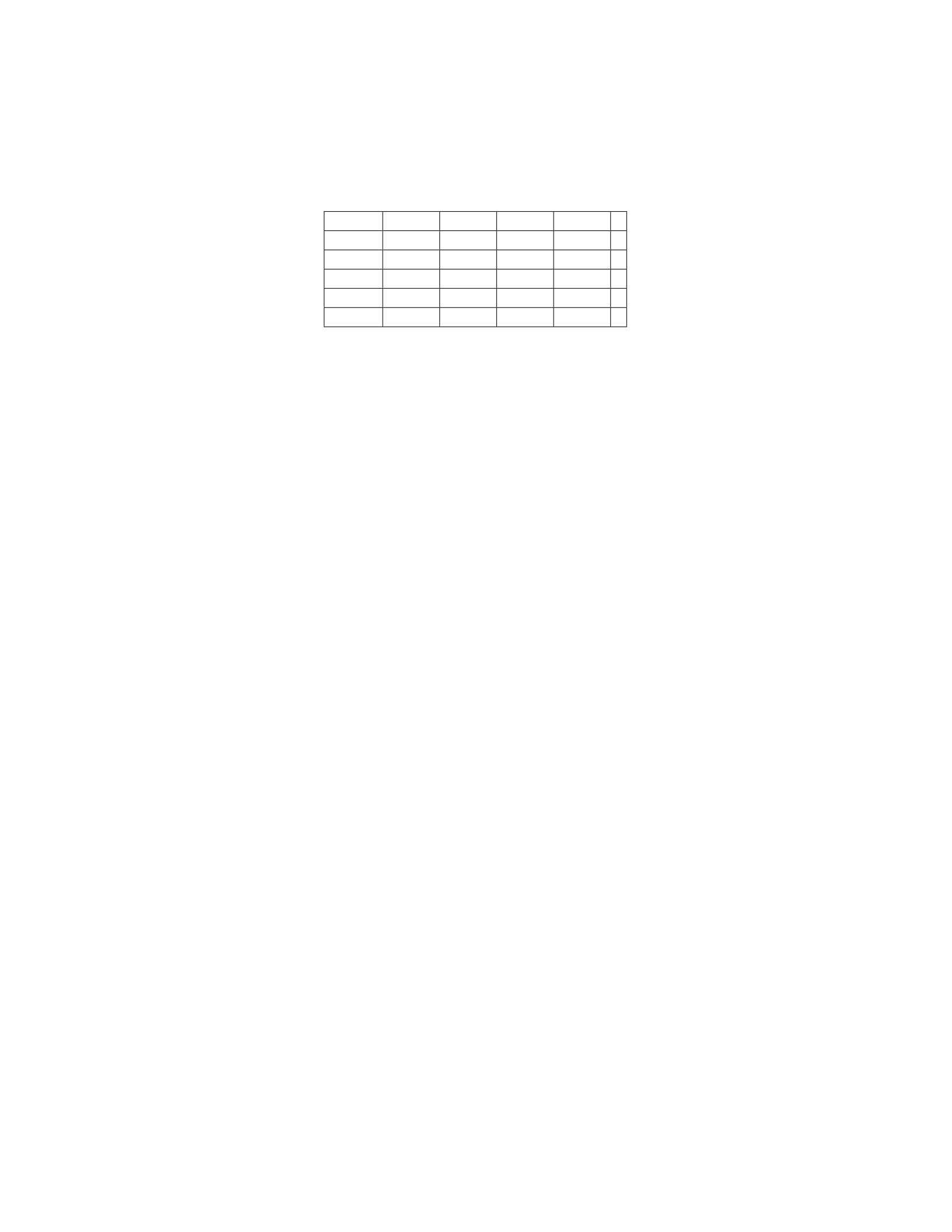
Y= 1 Y= 2 Y= 3 Y= 4
X= 1 0.05 0.10 0.05 0.10
X= 2 0.10 0.15 0.10 0.05
X= 3 0.20 0.15 0.05 0.00
X= 4 0.05 0.10 0.15 0.10
X= 5 0.00 0.00 0.10 0.15
Determine the least squares estimate of the regression coefficients β0and β1
in the simple linear regression model E(Y|X) = β0+β1X.
Solution
Step 1: Calculate the marginal probabilities of Xand Y.
The marginal probability mass function of Xis given by
pX(x) = ∑
y
pXY (x, y) = ∑
y
P(X=x, Y =y)
The marginal probability mass function of Yis given by
pY(y) = ∑
x
pXY (x, y) = ∑
x
P(X=x, Y =y)
Calculating these values gives: pX(1) = 0.30, pX(2) = 0.40, pX(3) =
0.40, pX(4) = 0.40, pX(5) = 0.25
pY(1) = 0.30, pY(2) = 0.35, pY(3) = 0.45, pY(4) = 0.40
Step 2: Calculate the sample means of Xand Y.
The sample means are given by
¯
X=
5
∑
i=1
xipX(xi),¯
Y=
4
∑
j=1
yjpY(yj)
Calculating these values gives: ¯
X= 3.45,¯
Y= 2.55
Step 3: Calculate the sample covariance and variance.
The sample covariance is given by
Cov(X, Y ) =
5
∑
i=1
4
∑
j=1
(xi−¯
X)(yj−¯
Y)pXY (xi, yj)
The sample variance is given by
Var(X) =
5
∑
i=1
(xi−¯
X)2pX(xi),Var(Y) =
4
∑
j=1
(yj−¯
Y)2pY(yj)
After calculating these values, we find: Cov(X, Y )=0.35,Var(X) =
1.2275,Var(Y) = 1.3475
21

Step 4: Calculate the least squares estimates.
The least squares estimates of the regression coefficients are given by
ˆ
β1=Cov(X, Y )
Var(X),ˆ
β0=¯
Y−ˆ
β1¯
X
Substitute the values we calculated above: ˆ
β1=0.35
1.2275 ≈0.2854,ˆ
β0= 2
Question 23
Question
Let y1, y2, y3, y4be a random sample from a normal distribution with unknown
mean µand unknown variance σ2. Consider the following estimator for µ:
ˆµ=1
4(y1+y2+y3+y4)
Show that ˆµis an unbiased estimator of µ.
Solution
Step 1: We need to show that E(ˆµ) = µ
Step 2: By linearity of expectation, we have:
E(ˆµ) = E(1
4(y1+y2+y3+y4))
Step 3: Since expectation is a linear operator, we can write this as:
1
4E(y1) + 1
4E(y2) + 1
4E(y3) + 1
4E(y4)
Step 4: Since y1, y2, y3, y4are from a normal distribution with mean µ, we
have E(yi) = µfor i= 1,2,3,4.
Step 5: Substituting this back into our expression, we get:
1
4(µ+µ+µ+µ) = µ
Step 6: Therefore, E(ˆµ) = µ, which means ˆµis an unbiased estimator of µ.
Question 24
Question
Suppose we have a dataset with the following values of independent variable x
and dependent variable y:
22

x1 2 3 4 5
y3 6 7 11 14
a) Find the least squares regression line that best fits the data.
b) Use the regression line to estimate the value of ywhen x= 6.
Solution
a) To find the least squares regression line, we need to calculate the slope and
intercept that minimize the sum of squared differences between the observed y
values and the predicted values from the regression line.
Step 1: Compute the means of xand yThe means of xand yare given
by:
¯x=1+2+3+4+5
5= 3
¯y=3+6+7+11+14
5= 8.2
Step 2: Calculate the slope of the regression line (b)The formula for
the slope of the least squares regression line is given by:
b=∑n
i=1(xi−¯x)(yi−¯y)
∑n
i=1(xi−¯x)2
where nis the number of data points. Calculating the numerator and denomi-
nator separately:
Numerator = (1 −3)(3 −8.2) + (2 −3)(6 −8.2) + (3 −3)(7 −8.2)
+ (4 −3)(11 −8.2) + (5 −3)(14 −8.2)
=−11.4
Denominator = (1 −3)2+ (2 −3)2+ (3 −3)2+ (4 −3)2+ (5 −3)2
= 10
Therefore, the slope bis given by:
b=−11.4
10 =−1.14
Step 3: Calculate the intercept of the regression line (a)The formula
for the intercept is:
a= ¯y−b¯x
Substitute the values of ¯y,b, and ¯xto find a:
a= 8.2−(−1.14 ×3) = 11.64
Hence, the least squares regression line is given by:
ˆy= 11.64 −1.14x
23

Question 25
Question
Let y=
−1
1
2
and X=
1 1
1 2
1 3
. Find the least squares estimate of βin the
model y=Xβ +ϵ, where ϵ=
1
−1
0
.
Solution
Step 1: Calculate the matrix product XTX.
XTX=(1 1 1
1 2 3)
1 1
1 2
1 3
=(3 6
6 14)
Step 2: Calculate the matrix product XTy.
XTy=(111
123)
−1
1
2
=(2
3)
Step 3: Solve the normal equations XTXˆ
β=XTyfor ˆ
β.
(3 6
6 14)ˆ
β=(2
3)
Step 4: Solve the system of equations to find ˆ
β.
{3ˆ
β1+ 6 ˆ
β2= 2
6ˆ
β1+ 14 ˆ
β2= 3
Solving these equations gives ˆ
β1=−1and ˆ
β2= 1/2.
Therefore, the least squares estimate of βis ˆ
β=(−1
1/2).
24

Step 2: Next, we calculate the deviations from the means for each month:
dX=X−¯
X= (2 −5) (4 −5) (6 −5)
(5 −5) (8 −5) (7 −5)
=−3−1
1 0 3
dY=Y−¯
Y= (3 −6.33) (5 −6.33) (7 −6.33)
(6 −6.33) (9 −6.33) (8 −6.33)
=−3.33 −1.33
0.67 −0.33 2.67
Step 3: Now, we calculate the sum of the products of the deviations:
∑dXdY= (−3)(−3.33) + (−1)(−1.33) + (1)(0.67) + (0)(−0.33) + (3)(2.67)
∑dXdY= 9.99 + 1.33 + 0.67+0+8.01 = 19
Step 4: Calculate the sum of the squares of the deviations of X:
∑d2
X= (−3)2+ (−1)2+ (1)2+ (0)2+ (3)2= 3 + 1 + 1 + 0 + 9 = 14
Step 5: The least squares estimates of the coefficients are:
ˆ
β1=∑dXdY
∑d2
X
=19
14 ≈1.36
ˆ
β0=¯
Y−ˆ
β1¯
X= 6.33 −1.36 ×5≈ −0.33
Therefore, the least squares estimate of the regression line is ˆ
Y≈ −0.33 +
1.36X.
Question 3
Question
Suppose we have a dataset with the following pairs of data: (x1, y1) = (2,5),
(x2, y2) = (4,9),(x3, y3) = (6,11), and (x4, y4) = (8,14). We want to model
the relationship between xand yusing a linear regression model of the form
ˆy=β0+β1x. Find the regression coefficients β0and β1using the method of
least squares estimation.
Solution
Step 1: Compute the means of xand y. The means are given by:
¯x=1
4(2 + 4 + 6 + 8) = 5
2

¯y=1
4(5 + 9 + 11 + 14) = 9.75
Step 2: Compute the sample variances of xand y. The sample variances are
given by:
s2
x=1
3
4
∑
i=1
(xi−¯x)2=1
3[(2 −5)2+ (4 −5)2+ (6 −5)2+ (8 −5)2] = 6.67
s2
y=1
3
4
∑
i=1
(yi−¯y)2=1
3[(5−9.75)2+(9−9.75)2+(11−9.75)2+(14−9.75)2]≈13.46
Step 3: Compute the sample covariance of xand y. The sample covariance
is given by:
sxy =1
3
4
∑
i=1
(xi−¯x)(yi−¯y) = 1
3[(2−5)(5−9.75)+(4−5)(9−9.75)+(6−5)(11−9.75)+(8−5)(14−9.75)] ≈9.25
Step 4: Compute the regression coefficients β0and β1. The slope β1is
calculated as:
β1=sxy
s2
x
≈9.25
6.67 ≈1.39
The intercept β0is then found from:
β0= ¯y−β1¯x= 9.75 −1.39 ×5≈2.90
Therefore, the estimated regression model is ˆy= 2.90 + 1.39x.
Question 4
Question
Let X=
1 3
1 4
1 5
1 6
and Y=
2
4
6
8
. Find the least squares estimate of the vector
β=(β0
β1)in the linear regression model Y=Xβ +εwhere ε∼N(0, σ2I).
Solution
Step 1: The least squares estimate of βis given by ˆ
β= (XTX)−1XTY.
Step 2: First, we calculate XTX:
XTX=(1111
3456)
1 3
1 4
1 5
1 6
=(4 18
18 86)
3

Step 3: Next, we calculate XTY:
XTY=(1 1 1 1
3 4 5 6)
2
4
6
8
=(20
80)
Step 4: Now, we find (XTX)−1:
(XTX)−1=(4 18
18 86)−1
=1
4·86 −18 ·18 (86 −18
−18 4 )
=1
308 (86 −18
−18 4 )
Step 5: Finally, we calculate ˆ
β:
ˆ
β=1
308 (86 −18
−18 4 )(20
80)=1
308 (1592
232 )=(5.16
0.75)
Therefore, the least squares estimate of βis ˆ
β=(5.16
0.75).
Question 5
Question
Let Y1, Y2, . . . , Ynbe a random sample from a normal population with mean µ
and variance σ2. Consider the simple linear regression model
Yi=β0+β1xi+εi
where εi’s are independent N(0, σ2)random variables.
Show that the least squares estimators ˆ
β0and ˆ
β1are unbiased for β0and
β1, respectively.
Solution
Step 1: To show that ˆ
β0is an unbiased estimator for β0, we need to find E(ˆ
β0)
and show that it equals β0.
E(ˆ
β0) = E(¯
Y−ˆ
β1¯x)=E(1
n
n
∑
i=1
Yi−ˆ
β1
1
n
n
∑
i=1
xi)
4

Step 2: Since ¯
Y=¯
β0+¯
β1¯x, we can expand the expression.
E(ˆ
β0) = 1
n
n
∑
i=1
E(Yi)−ˆ
β1
1
n
n
∑
i=1
E(xi)
Step 3: Since Yifollows a normal distribution with mean µ,E(Yi) = µ. Also,
E(xi) = E(x) = µx.
E(ˆ
β0) = 1
n
n
∑
i=1
µ−ˆ
β1
1
n
n
∑
i=1
µx
Step 4: Simplifying the expression further, we get
E(ˆ
β0) = µ−ˆ
β1µx
Step 5: Since µ=β0and µxis the true mean of x, we have E(ˆ
β0) = β0.
This shows that ˆ
β0is an unbiased estimator for β0.
Step 6: Similarly, we can show that ˆ
β1is an unbiased estimator for β1by
finding E(ˆ
β1)and showing that it equals β1.
Therefore, both least squares estimators ˆ
β0and ˆ
β1are unbiased for β0and
β1, respectively.
Question 6
Question
Let X=
1 1
1 2
1 3
1 4
be the design matrix for a linear regression problem with
response vector Y=
2
4
5
7
. Find the least squares estimate of the regression
coefficients.
Solution
Step 1: The least squares estimate of the regression coefficients ˆ
βis given by
the formula: ˆ
β= (XTX)−1XTY
Step 2: First, calculate XTXby multiplying XTand X:
XT=(1 1 1 1
1 2 3 4)
5

XTX=(1111
1234)
1 1
1 2
1 3
1 4
=(4 10
10 30)
Step 3: Next, calculate XTYby multiplying XTand Y:
Y=
2
4
5
7
XTY=(1 1 1 1
1 2 3 4)
2
4
5
7
=(18
46)
Step 4: Now, calculate (XTX)−1by finding the inverse of XTX:
(XTX)−1=(4 10
10 30)−1
=(3
20 −1
10
−1
10
2
5)
Step 5: Finally, calculate the least squares estimate of the regression coeffi-
cients ˆ
β:
ˆ
β= (XTX)−1XTY=(3
20 −1
10
−1
10
2
5)(18
46)=(2
1)
Therefore, the least squares estimate of the regression coefficients is ˆ
β=
(2
1).
Question 7
Question
Let Yi=a+bXi+eibe a simple linear regression model where Yirepresents
the response variable, Xirepresents the predictor variable, arepresents the
intercept, brepresents the slope, and eirepresents the error term for the ith
observation. Consider the following data points:
X Y
1 4
2 7
3 8
4 11
Determine the least squares estimation for the coefficients aand bin the model.
6

Solution
Step 1: Calculate the means of Xand Y. The means are given by:
¯
X=1+2+3+4
4= 2.5
¯
Y=4+7+8+11
4= 7.5
Step 2: Calculate the sum of products and sum of squares. We need to
calculate: n
∑
i=1
XiYi,
n
∑
i=1
X2
i,and
n
∑
i=1
Y2
i
Substitute the given values:
∑XiYi= 1 ∗4+2∗7+3∗8+4∗11 = 4 + 14 + 24 + 44 = 86
∑X2
i= 12+ 22+ 32+ 42= 1 + 4 + 9 + 16 = 30
∑Y2
i= 42+ 72+ 82+ 112= 16 + 49 + 64 + 121 = 250
Step 3: Calculate the least squares estimations for aand b. The least squares
estimators for the coefficients aand bare given by:
b=n∑XiYi−∑Xi∑Yi
n∑X2
i−(∑Xi)2
a=¯
Y−b¯
X
Substitute the calculated values:
b=4∗86 −10 ∗30
4∗30 −102=344 −300
120 −100 =44
20 = 2.2
a= 7.5−2.2∗2.5 = 7.5−5.5 = 2
Therefore, the least squares estimations for the coefficients aand bare a= 2
and b= 2.2.
Question 8
Question
A researcher is interested in examining the relationship between the number of
hours spent studying for an exam and the exam score received. The researcher
collects data from 10 students and obtains the following results:
7

Hours Studied (x) Exam Score (y)
1 60
2 65
3 71
4 73
5 76
6 79
7 82
8 85
9 88
10 91
Using the least squares estimation method, find the equation of the regression
line that best represents the relationship between the hours studied and the
exam score.
Solution
Step 1: Calculate ¯x,¯y,SSxx, and SSxy .
¯x=1+2+3+4+5+6+7+8+9+10
10 = 5.5
¯y=60+65+71+73+76+79+82+85+88+91
10 = 78
SSxx =
10
∑
i=1
(xi−¯x)2=
10
∑
i=1
(xi−5.5)2= 82.5
SSxy =
10
∑
i=1
(xi−¯x)(yi−¯y) =
10
∑
i=1
(xi−5.5)(yi−78) = 199.5
Step 2: Calculate the slope (b) and intercept (a) of the regression line.
b=SSxy
SSxx
=199.5
82.5≈2.42
a= ¯y−b¯x= 78 −2.42 ×5.5≈65.09
Step 3: Formulate the equation of the regression line. The equation of the
regression line is given by y=a+bx. Substituting the values of aand b:
y= 65.09 + 2.42x
Therefore, the equation of the regression line that best represents the rela-
tionship between the hours studied and the exam score is y= 65.09 + 2.42x.
8

Question 9
Question
Suppose we have a set of data points (x1, y1),(x2, y2),(x3, y3),(x4, y4)where xi
represents the independent variable and yirepresents the dependent variable.
We want to fit a linear regression model y=β0+β1xto this data. The normal
equations for this model are as follows:
nˆ
β0+(∑xi)ˆ
β1=∑yi
(∑xi)ˆ
β0+(∑x2
i)ˆ
β1=∑xiyi
Given the data points (1,3),(2,4),(3,5),(4,6), find the least squares esti-
mates ˆ
β0and ˆ
β1.
Solution
Step 1: Substitute the given data points (xi, yi)into the normal equations:
First equation:
4ˆ
β0+ 10 ˆ
β1= 18
Second equation:
10 ˆ
β0+ 30 ˆ
β1= 44
Step 2: Solve the system of equations to find ˆ
β0and ˆ
β1.
Multiplying the first equation by 3 and subtracting the second equation from
the result:
12 ˆ
β0+ 30 ˆ
β1−10 ˆ
β0−30 ˆ
β1= 54 −44
2ˆ
β0= 10
ˆ
β0= 5
Substitute ˆ
β0= 5 into the first equation:
4(5) + 10 ˆ
β1= 18
20 + 10 ˆ
β1= 18
10 ˆ
β1=−2
ˆ
β1=−0.2
Therefore, the least squares estimates are ˆ
β0= 5 and ˆ
β1=−0.2.
9

Question 10
Question
Let X=
1 1
1 2
1 3
1 4
be the design matrix and y=
2
3
3
4
be the response vector.
Find the least squares estimate of the coefficient vector βin the linear regression
model Y=Xβ +ϵ.
Solution
Step 1: Calculate XTX.
XTX=[1111
1234]
1 1
1 2
1 3
1 4
=[4 10
10 30]
Step 2: Calculate (XTX)−1.
(XTX)−1=[4 10
10 30]−1
=1
4∗30 −10 ∗10 [30 −10
−10 4 ]=[3
40 −1
20
−1
20
1
10 ]
Step 3: Calculate XTy.
XTy=[1111
1234]
2
3
3
4
=[12
30]
Step 4: Calculate the least squares estimate of β, denoted as ˆ
β.
ˆ
β= (XTX)−1XTy=[3
40 −1
20
−1
20
1
10 ][12
30]=[9
10
15
10 ]=[0.9
1.5]
Therefore, the least squares estimate of the coefficient vector βin the linear
regression model is ˆ
β=[0.9
1.5].
Question 11
Question
Suppose we have a dataset with the following five data points: (1, 3), (2, 5), (3,
7), (4, 9), (5, 11). We want to fit a linear regression model to this dataset using
the method of least squares estimation. Find the equation of the regression line
that best fits the data.
10

Solution
Step 1: Calculate the mean of the x-values (¯x) and the mean of the y-values
(¯y). To find ¯xand ¯y, we sum up all the x-values and y-values respectively and
then divide by the total number of data points (in this case, 5).
¯x=1+2+3+4+5
5=15
5= 3
¯y=3+5+7+9+11
5=35
5= 7
Step 2: Calculate the slope (b) of the regression line using the least squares
estimation formula:
b=∑n
i=1(xi−¯x)(yi−¯y)
∑n
i=1(xi−¯x)2
Substitute the given data points and ¯xand ¯yvalues into the formula to
calculate b.
b=(1 −3)(3 −7) + (2 −3)(5 −7) + (3 −3)(7 −7) + (4 −3)(9 −7) + (5 −3)(11 −7)
(1 −3)2+ (2 −3)2+ (3 −3)2+ (4 −3)2+ (5 −3)2
b=(−2)(−4) + (−1)(−2) + (0)(0) + (1)(2) + (2)(4)
(−2)2+ (−1)2+ (0)2+ (1)2+ (2)2
b=8+2+0+2+8
4+1+0+1+4
b=20
10 = 2
Step 3: Calculate the y-intercept (a) of the regression line using the formula:
a= ¯y−b¯x
Substitute the calculated values of ¯x,¯y, and binto the formula to find a.
a= 7 −2×3 = 7 −6 = 1
Step 4: Write the equation of the regression line in the form y=a+bx using
the calculated values of aand b.
y= 1 + 2x
Therefore, the equation of the regression line that best fits the data points
(1, 3), (2, 5), (3, 7), (4, 9), (5, 11) is y= 1 + 2x.
Question 12
Question
Suppose we have a dataset with the following pairs of observations: (x1, y1) =
(1,3),(x2, y2) = (2,7),(x3, y3) = (3,5),(x4, y4) = (4,10). Consider the linear
model Y=β0+β1X+ε, where ε∼N(0, σ2). Find the least squares estimates
of β0and β1.
11

Solution
Step 1: The model we’re considering is:
Y=β0+β1X+ε
Step 2: The least squares estimates of β0and β1are obtained by minimizing
the sum of squared residuals. The residual for the ith observation is given by
ei=yi−(ˆ
β0+ˆ
β1xi).
Step 3: The sum of squared residuals is:
Q(β0, β1) =
n
∑
i=1
e2
i=
n
∑
i=1
(yi−β0−β1xi)2
Step 4: To find the least squares estimates, we differentiate Qwith respect to
β0and β1and set the derivatives equal to zero to obtain the normal equations.
Solving these equations will give us the estimates.
Step 5: The normal equations are:
∂Q
∂β0
=−2
n
∑
i=1
(yi−β0−β1xi) = 0
∂Q
∂β1
=−2
n
∑
i=1
xi(yi−β0−β1xi) = 0
Step 6: Substituting the observed values, we have:
−4(∑yi)+4nβ0+ 10β1= 0
−2(∑xiyi)+4β0+ 14β1= 0
Step 7: Solving these equations simultaneously, we get:
ˆ
β0=35
6
ˆ
β1=15
8
Step 8: Therefore, the least squares estimates of β0and β1are ˆ
β0=35
6and
ˆ
β1=15
8.
Question 13
Question
Let Y=
3
2
1
be the response vector and X=
1 1
1 2
1 3
be the design matrix
in a simple linear regression model Y=β0+β1X+ε. Find the least squares
estimates ˆ
β0and ˆ
β1.
12

Solution
Step 1: The least squares estimates ˆ
β0and ˆ
β1are given by the formulas:
ˆ
β= (X⊺X)−1X⊺Y
Step 2: Let’s start by computing X⊺X, where X⊺is the transpose of X:
X⊺=(111
123)
Step 3: Next, we multiply X⊺by X:
X⊺X=(111
123)
1 1
1 2
1 3
=(3 6
6 14)
Step 4: Now, calculate X⊺Y:
X⊺Y=(1 1 1
1 2 3)
3
2
1
=(6
10)
Step 5: Using the formula ˆ
β= (X⊺X)−1X⊺Y:
ˆ
β=(3 6
6 14)−1(6
10)
Step 6: Solving for ˆ
βyields:
ˆ
β=(−2 1
1.5−0.5)(6
10)=(−2
3)
Therefore, the least squares estimates are ˆ
β0=−2and ˆ
β1= 3.
Question 14
Question
Let Xbe an n×pmatrix and Ybe an n×1matrix. Suppose that the model
Y=Xβ +ϵholds, where ϵ∼N(0, σ2I), and βis the p×1unknown coefficient
vector. Prove that the least squares estimator of β, denoted by ˆ
β, is the solution
to the normal equations XT(Y−Xˆ
β) = 0.
13

Solution
Step 1: Given the least squares estimation of β, we have:
ˆ
β= (XTX)−1XTY
Step 2: To prove that ˆ
βis the solution to the normal equations XT(Y−
Xˆ
β) = 0, we substitute the expression for ˆ
βinto the normal equations:
XT(Y−Xˆ
β) = XT(Y−X(XTX)−1XTY)
Step 3: Expand the terms:
=XTY−XTX(XTX)−1XTY
Step 4: Since (XTX)−1XTX=I, where Iis the identity matrix, the above
expression simplifies to:
=XTY−XTY
Step 5: This simplifies further to:
= 0
Step 6: Therefore, the least squares estimator of β,ˆ
β, is indeed the solution
to the normal equations XT(Y−Xˆ
β) = 0.
Question 15
Question
Let X=
1 1
1−1
1 2
and y=
2
3
1
. Find the least squares estimate of the
column vector βminimizing ||y−Xβ||2.
Solution
Step 1: Calculate XTX.
XTX=(1 1 1
1−1 2)
1 1
1−1
1 2
=(3 1
1 6)
Step 2: Calculate XTy.
XTy=(1 1 1
1−1 2)
2
3
1
=(6
3)
14

Step 3: Solve for ˆ
βby solving the normal equations XTXˆ
β=XTy.
(3 1
1 6)ˆ
β=(6
3)
(3 1
1 6)ˆ
β=(6
3)
Step 4: Solve the system of equations to find ˆ
β.
3ˆ
β1+ˆ
β2= 6
ˆ
β1+ 6 ˆ
β2= 3
Step 5: Solving the system of equations gives ˆ
β1=11
17 and ˆ
β2=9
17 . There-
fore, the least squares estimate of the column vector βis ˆ
β=(11
17
9
17 ).
Question 16
Question
Suppose we have a dataset with the following pairs of values:
x y
1 2
2 3
3 3
4 5
5 4
6 7
Using the least squares method, find the best-fit line for this dataset.
Solution
Step 1: Calculate the mean of xand y: The mean of xis calculated as:
¯x=1+2+3+4+5+6
6=21
6= 3.5
The mean of yis calculated as:
¯y=2+3+3+5+4+7
6=24
6= 4
Step 2: Calculate the covariance and variance of xand y: The covariance of
xand yis calculated as:
Cov(x, y) = ∑n
i=1(xi−¯x)(yi−¯y)
n−1
15

Substitute the values from our dataset:
Cov(x, y) = (1 −3.5)(2 −4) + (2 −3.5)(3 −4) + (3 −3.5)(3 −4) + (4 −3.5)(5 −4) + (5 −3.5)(4 −4) + (6 −3.5)(7 −4)
6−1
Cov(x, y) = (−2.5)(−2) + (−1.5)(−1) + (−0.5)(−1) + (0.5)(1) + (1.5)(0) + (2.5)(3)
5
Cov(x, y) = 5+1.5+0.5+0.5+0−7.5
5=−1
5=−0.2
The variance of xis calculated as:
Var(x) = ∑n
i=1(xi−¯x)2
n−1
Substitute the values from our dataset:
Var(x) = (1 −3.5)2+ (2 −3.5)2+ (3 −3.5)2+ (4 −3.5)2+ (5 −3.5)2+ (6 −3.5)2
6−1
Var(x) = 6.25 + 2.25 + 0.25 + 0.25 + 2.25 + 6.25
5=17.5
5= 3.5
The covariance of yis equal to the variance of y, which is calculated similarly
as:
Var(y) = ∑n
i=1(yi−¯y)2
n−1
Substitute the values from our dataset:
Var(y) = (2 −4)2+ (3 −4)2+ (3 −4)2+ (5 −4)2+ (4 −4)2+ (7 −4)2
6−1
Var(y) = 4+1+1+1+0+9
5=16
5= 3.2
Step 3: Calculate the slope and intercept of the best-fit line: The slope of
the best-fit line is given by:
b=Cov(x, y)
Var(x)
Substitute the calculated values:
b=−0.2
3.5=−1
17.5
The intercept of the best-fit line is given by:
a= ¯y
16

Question 17
Question
Suppose we have a dataset with the following observations for two variables X
and Y:
X Y
1 2
2 3
3 4
4 5
5 7
Calculate the least squares estimates of the intercept and slope for the simple
linear regression model Y=β0+β1X.
Solution
Step 1: Calculate the means of Xand Y:
The mean of Xis ¯
X=1+2+3+4+5
5= 3.
The mean of Yis ¯
Y=2+3+4+5+7
5=21
5= 4.2.
Step 2: Calculate the sums of squares:
SSXX =
n
∑
i=1
(Xi−¯
X)2= (1 −3)2+ (2 −3)2+ (3 −3)2+ (4 −3)2+ (5 −3)2= 10
SSXY =
n
∑
i=1
(Xi−¯
X)(Yi−¯
Y) = (1−3)(2−4.2)+(2−3)(3−4.2)+(3−3)(4−4.2)+(4−3)(5−4.2)+(5−3)(7−4.2) = 7.6
SSY Y =
n
∑
i=1
(Yi−¯
Y)2= (2−4.2)2+(3−4.2)2+(4−4.2)2+(5−4.2)2+(7−4.2)2= 10.8
Step 3: Calculate the least squares estimates:
The slope estimator is ˆ
β1=SSX Y
SSX X =7.6
10 = 0.76.
The intercept estimator is ˆ
β0=¯
Y−ˆ
β1¯
X= 4.2−0.76(3) = 1.92.
Therefore, the least squares estimates of the intercept and slope for the
simple linear regression model are ˆ
β0= 1.92 and ˆ
β1= 0.76, respectively.
Question 18
Question
Suppose we have data points (x1, y1),(x2, y2),(x3, y3),(x4, y4),and (x5, y5)where
xirepresents the independent variable and yirepresents the dependent variable.
17

The linear regression model is given by y=β0+β1x. Using the method of least
squares, find the values of β0and β1that minimize the sum of the squared
differences between the observed values yiand the predicted values ˆyi.
Given data points: (1,3),(2,6),(3,5),(4,10),and (5,8).
Solution
Step 1: The linear regression model can be written as:
ˆy=β0+β1x
Step 2: We want to minimize the sum of squared differences between the
observed yivalues and the predicted ˆyivalues, given by:
n
∑
i=1
(yi−ˆyi)2=
n
∑
i=1
(yi−β0−β1xi)2
Step 3: Substituting the given data points into the above equation, we get:
(3−β0−β1)2+(6−β0−2β1)2+(5−β0−3β1)2+(10−β0−4β1)2+(8−β0−5β1)2
Step 4: Expanding and simplifying the expression, we have:
To be continued...
Question 19
Question
Suppose we have a dataset with the following pairs of data points (xi, yi):
(1,2),(2,3),(3,4),(4,6),(5,6),(6,7)
Perform linear regression to find the least squares estimation of the line
y=mx +bthat best fits these data points.
Solution
Step 1: Calculate the means of xand y.
¯x=1+2+3+4+5+6
6=21
6= 3.5
¯y=2+3+4+6+6+7
6=28
6≈4.67
Step 2: Calculate the slope mand the y-intercept bof the least squares
regression line.
m=∑n
i=1(xi−¯x)(yi−¯y)
∑n
i=1(xi−¯x)2
18

b= ¯y−m¯x
Plugging in the given data points:
6
∑
i=1
(xi−¯x)(yi−¯y) = 7.83
6
∑
i=1
(xi−¯x)2= 8.67
Therefore,
m=7.83
8.67 ≈0.9057
b= 4.67 −0.9057 ·3.5≈1.43
Therefore, the least squares estimation of the line that best fits the given
data points is y= 0.9057x+ 1.43.
Question 20
Question
Let Ybe a dependent variable and Xan independent variable. Consider the
model Y=β0+β1X+ϵ, where ϵis the error term. Suppose the least squares
estimators of β0and β1are ˆ
β0= 3.2and ˆ
β1= 2.5.
Calculate the least squares estimate of Ywhen X= 4 and interpret the
result in the context of the problem.
Solution
Step 1: Substitute the estimated coefficients into the regression model. The
least squares estimate of Yis given by ˆ
Y=ˆ
β0+ˆ
β1X. Substitute ˆ
β0= 3.2and
ˆ
β1= 2.5into the equation:
ˆ
Y= 3.2+2.5×4
Step 2: Calculate the least squares estimate of Y.
ˆ
Y= 3.2+2.5×4 = 3.2 + 10 = 13.2
Therefore, the least squares estimate of Ywhen X= 4 is 13.2.
Step 3: Interpretation of the result. The estimated value of Y(13.2) when
X= 4 suggests that, based on the linear regression model, when the independent
variable Xis equal to 4, the estimated value of the dependent variable Yis 13.2.
This implies that for every unit increase in X,Yis estimated to increase by 2.5
units, holding all else constant.
19

Question 21
Question
Suppose we have a dataset with the following 5 data points: (-2, 1), (-1, 3), (0,
2), (1, 5), (2, 7). We want to perform linear regression to find the best-fitting
line through these points using the least squares method. Find the equation of
the regression line and determine the coefficient of determination R2.
Solution
Step 1: Let’s start by setting up the least squares regression model. The equa-
tion of a linear regression model is given by Y=β0+β1X+ε, where β0is the
y-intercept, β1is the slope, Xis the independent variable, and εis the error
term.
Step 2: We want to find the values of β0and β1that minimize the sum
of the squared residuals. The sum of squared residuals is given by SSres =
∑n
i=1(Yi−(β0+β1Xi))2.
Step 3: We can expand the expression for SSres using the given data points.
Substituting the data points into the sum gives us: SSres = (1 −(β0−2β1))2+
(3 −(β0−β1))2+ (2 −β0)2+ (5 −(β0+β1))2+ (7 −(β0+ 2β1))2.
Step 4: To find the values of β0and β1that minimize SSres, we need to take
partial derivatives of SSres with respect to β0and β1, set them equal to 0, and
solve the resulting system of equations.
Step 5: After solving the system of equations, we find that the least squares
regression line is Y=15
4+7
4X.
Step 6: To determine the coefficient of determination R2, we need to cal-
culate the total sum of squares SStotal and the coefficient of determination R2
using the following formulas: SStotal =∑n
i=1(Yi−¯
Y)2and R2= 1 −SSres
SStotal .
Step 7: Substituting the values into the formulas, we can calculate SStotal
and R2. After the calculations, we find R2= 0.964.
Therefore, the equation of the regression line through the given data points
is Y=15
4+7
4X, and the coefficient of determination R2is 0.964.
Question 22
Question
Let Xbe a random variable with values in {1,2,3,4,5}and let Ybe a ran-
dom variable with values in {1,2,3,4}. The following table shows the joint
probabilities of Xand Y:
20
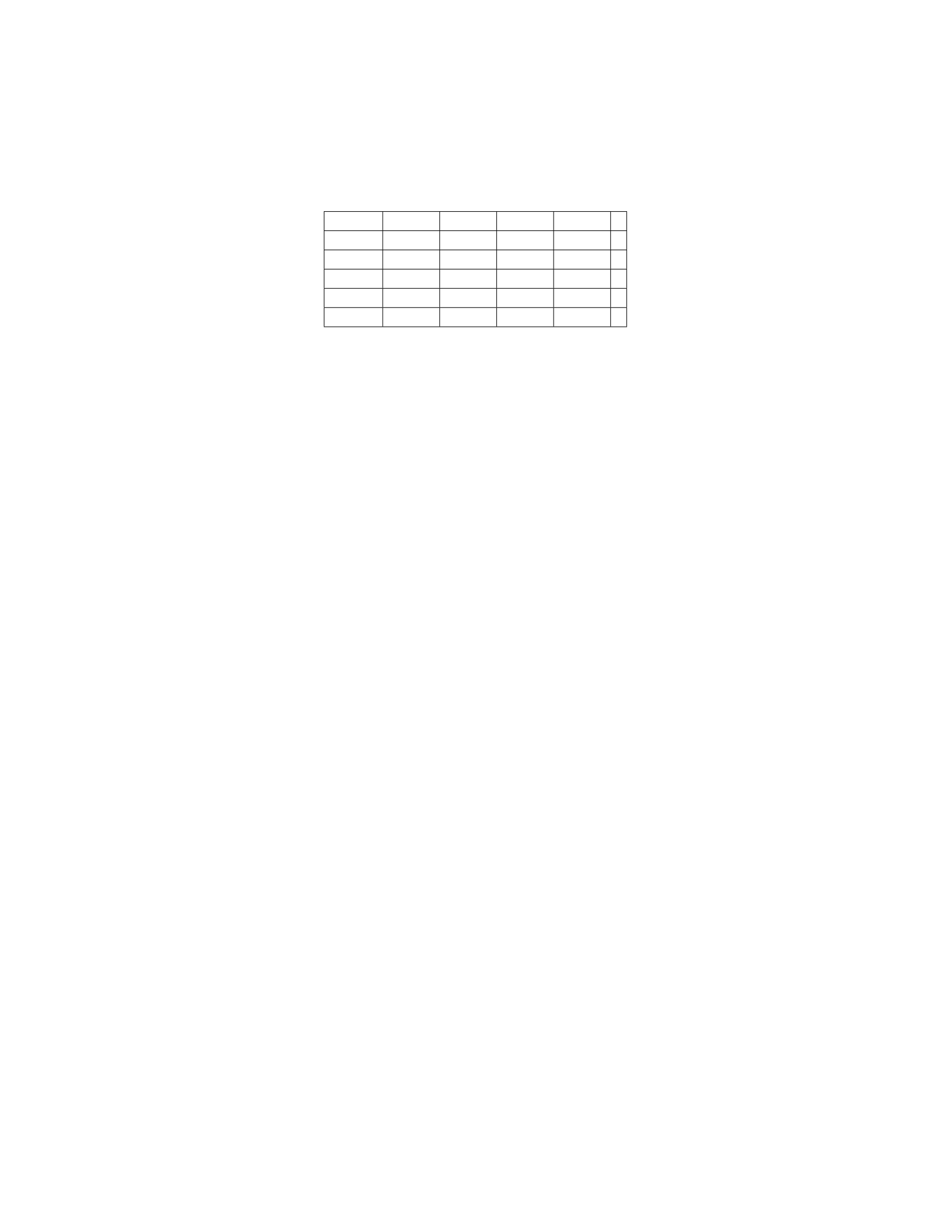
Y= 1 Y= 2 Y= 3 Y= 4
X= 1 0.05 0.10 0.05 0.10
X= 2 0.10 0.15 0.10 0.05
X= 3 0.20 0.15 0.05 0.00
X= 4 0.05 0.10 0.15 0.10
X= 5 0.00 0.00 0.10 0.15
Determine the least squares estimate of the regression coefficients β0and β1
in the simple linear regression model E(Y|X) = β0+β1X.
Solution
Step 1: Calculate the marginal probabilities of Xand Y.
The marginal probability mass function of Xis given by
pX(x) = ∑
y
pXY (x, y) = ∑
y
P(X=x, Y =y)
The marginal probability mass function of Yis given by
pY(y) = ∑
x
pXY (x, y) = ∑
x
P(X=x, Y =y)
Calculating these values gives: pX(1) = 0.30, pX(2) = 0.40, pX(3) =
0.40, pX(4) = 0.40, pX(5) = 0.25
pY(1) = 0.30, pY(2) = 0.35, pY(3) = 0.45, pY(4) = 0.40
Step 2: Calculate the sample means of Xand Y.
The sample means are given by
¯
X=
5
∑
i=1
xipX(xi),¯
Y=
4
∑
j=1
yjpY(yj)
Calculating these values gives: ¯
X= 3.45,¯
Y= 2.55
Step 3: Calculate the sample covariance and variance.
The sample covariance is given by
Cov(X, Y ) =
5
∑
i=1
4
∑
j=1
(xi−¯
X)(yj−¯
Y)pXY (xi, yj)
The sample variance is given by
Var(X) =
5
∑
i=1
(xi−¯
X)2pX(xi),Var(Y) =
4
∑
j=1
(yj−¯
Y)2pY(yj)
After calculating these values, we find: Cov(X, Y )=0.35,Var(X) =
1.2275,Var(Y) = 1.3475
21

Step 4: Calculate the least squares estimates.
The least squares estimates of the regression coefficients are given by
ˆ
β1=Cov(X, Y )
Var(X),ˆ
β0=¯
Y−ˆ
β1¯
X
Substitute the values we calculated above: ˆ
β1=0.35
1.2275 ≈0.2854,ˆ
β0= 2
Question 23
Question
Let y1, y2, y3, y4be a random sample from a normal distribution with unknown
mean µand unknown variance σ2. Consider the following estimator for µ:
ˆµ=1
4(y1+y2+y3+y4)
Show that ˆµis an unbiased estimator of µ.
Solution
Step 1: We need to show that E(ˆµ) = µ
Step 2: By linearity of expectation, we have:
E(ˆµ) = E(1
4(y1+y2+y3+y4))
Step 3: Since expectation is a linear operator, we can write this as:
1
4E(y1) + 1
4E(y2) + 1
4E(y3) + 1
4E(y4)
Step 4: Since y1, y2, y3, y4are from a normal distribution with mean µ, we
have E(yi) = µfor i= 1,2,3,4.
Step 5: Substituting this back into our expression, we get:
1
4(µ+µ+µ+µ) = µ
Step 6: Therefore, E(ˆµ) = µ, which means ˆµis an unbiased estimator of µ.
Question 24
Question
Suppose we have a dataset with the following values of independent variable x
and dependent variable y:
22

x1 2 3 4 5
y3 6 7 11 14
a) Find the least squares regression line that best fits the data.
b) Use the regression line to estimate the value of ywhen x= 6.
Solution
a) To find the least squares regression line, we need to calculate the slope and
intercept that minimize the sum of squared differences between the observed y
values and the predicted values from the regression line.
Step 1: Compute the means of xand yThe means of xand yare given
by:
¯x=1+2+3+4+5
5= 3
¯y=3+6+7+11+14
5= 8.2
Step 2: Calculate the slope of the regression line (b)The formula for
the slope of the least squares regression line is given by:
b=∑n
i=1(xi−¯x)(yi−¯y)
∑n
i=1(xi−¯x)2
where nis the number of data points. Calculating the numerator and denomi-
nator separately:
Numerator = (1 −3)(3 −8.2) + (2 −3)(6 −8.2) + (3 −3)(7 −8.2)
+ (4 −3)(11 −8.2) + (5 −3)(14 −8.2)
=−11.4
Denominator = (1 −3)2+ (2 −3)2+ (3 −3)2+ (4 −3)2+ (5 −3)2
= 10
Therefore, the slope bis given by:
b=−11.4
10 =−1.14
Step 3: Calculate the intercept of the regression line (a)The formula
for the intercept is:
a= ¯y−b¯x
Substitute the values of ¯y,b, and ¯xto find a:
a= 8.2−(−1.14 ×3) = 11.64
Hence, the least squares regression line is given by:
ˆy= 11.64 −1.14x
23

Question 25
Question
Let y=
−1
1
2
and X=
1 1
1 2
1 3
. Find the least squares estimate of βin the
model y=Xβ +ϵ, where ϵ=
1
−1
0
.
Solution
Step 1: Calculate the matrix product XTX.
XTX=(1 1 1
1 2 3)
1 1
1 2
1 3
=(3 6
6 14)
Step 2: Calculate the matrix product XTy.
XTy=(111
123)
−1
1
2
=(2
3)
Step 3: Solve the normal equations XTXˆ
β=XTyfor ˆ
β.
(3 6
6 14)ˆ
β=(2
3)
Step 4: Solve the system of equations to find ˆ
β.
{3ˆ
β1+ 6 ˆ
β2= 2
6ˆ
β1+ 14 ˆ
β2= 3
Solving these equations gives ˆ
β1=−1and ˆ
β2= 1/2.
Therefore, the least squares estimate of βis ˆ
β=(−1
1/2).
24

Step 2: Next, we calculate the deviations from the means for each month:
dX=X−¯
X= (2 −5) (4 −5) (6 −5)
(5 −5) (8 −5) (7 −5)
=−3−1
1 0 3
dY=Y−¯
Y= (3 −6.33) (5 −6.33) (7 −6.33)
(6 −6.33) (9 −6.33) (8 −6.33)
=−3.33 −1.33
0.67 −0.33 2.67
Step 3: Now, we calculate the sum of the products of the deviations:
∑dXdY= (−3)(−3.33) + (−1)(−1.33) + (1)(0.67) + (0)(−0.33) + (3)(2.67)
∑dXdY= 9.99 + 1.33 + 0.67+0+8.01 = 19
Step 4: Calculate the sum of the squares of the deviations of X:
∑d2
X= (−3)2+ (−1)2+ (1)2+ (0)2+ (3)2= 3 + 1 + 1 + 0 + 9 = 14
Step 5: The least squares estimates of the coefficients are:
ˆ
β1=∑dXdY
∑d2
X
=19
14 ≈1.36
ˆ
β0=¯
Y−ˆ
β1¯
X= 6.33 −1.36 ×5≈ −0.33
Therefore, the least squares estimate of the regression line is ˆ
Y≈ −0.33 +
1.36X.
Question 3
Question
Suppose we have a dataset with the following pairs of data: (x1, y1) = (2,5),
(x2, y2) = (4,9),(x3, y3) = (6,11), and (x4, y4) = (8,14). We want to model
the relationship between xand yusing a linear regression model of the form
ˆy=β0+β1x. Find the regression coefficients β0and β1using the method of
least squares estimation.
Solution
Step 1: Compute the means of xand y. The means are given by:
¯x=1
4(2 + 4 + 6 + 8) = 5
2

¯y=1
4(5 + 9 + 11 + 14) = 9.75
Step 2: Compute the sample variances of xand y. The sample variances are
given by:
s2
x=1
3
4
∑
i=1
(xi−¯x)2=1
3[(2 −5)2+ (4 −5)2+ (6 −5)2+ (8 −5)2] = 6.67
s2
y=1
3
4
∑
i=1
(yi−¯y)2=1
3[(5−9.75)2+(9−9.75)2+(11−9.75)2+(14−9.75)2]≈13.46
Step 3: Compute the sample covariance of xand y. The sample covariance
is given by:
sxy =1
3
4
∑
i=1
(xi−¯x)(yi−¯y) = 1
3[(2−5)(5−9.75)+(4−5)(9−9.75)+(6−5)(11−9.75)+(8−5)(14−9.75)] ≈9.25
Step 4: Compute the regression coefficients β0and β1. The slope β1is
calculated as:
β1=sxy
s2
x
≈9.25
6.67 ≈1.39
The intercept β0is then found from:
β0= ¯y−β1¯x= 9.75 −1.39 ×5≈2.90
Therefore, the estimated regression model is ˆy= 2.90 + 1.39x.
Question 4
Question
Let X=
1 3
1 4
1 5
1 6
and Y=
2
4
6
8
. Find the least squares estimate of the vector
β=(β0
β1)in the linear regression model Y=Xβ +εwhere ε∼N(0, σ2I).
Solution
Step 1: The least squares estimate of βis given by ˆ
β= (XTX)−1XTY.
Step 2: First, we calculate XTX:
XTX=(1111
3456)
1 3
1 4
1 5
1 6
=(4 18
18 86)
3

Step 3: Next, we calculate XTY:
XTY=(1 1 1 1
3 4 5 6)
2
4
6
8
=(20
80)
Step 4: Now, we find (XTX)−1:
(XTX)−1=(4 18
18 86)−1
=1
4·86 −18 ·18 (86 −18
−18 4 )
=1
308 (86 −18
−18 4 )
Step 5: Finally, we calculate ˆ
β:
ˆ
β=1
308 (86 −18
−18 4 )(20
80)=1
308 (1592
232 )=(5.16
0.75)
Therefore, the least squares estimate of βis ˆ
β=(5.16
0.75).
Question 5
Question
Let Y1, Y2, . . . , Ynbe a random sample from a normal population with mean µ
and variance σ2. Consider the simple linear regression model
Yi=β0+β1xi+εi
where εi’s are independent N(0, σ2)random variables.
Show that the least squares estimators ˆ
β0and ˆ
β1are unbiased for β0and
β1, respectively.
Solution
Step 1: To show that ˆ
β0is an unbiased estimator for β0, we need to find E(ˆ
β0)
and show that it equals β0.
E(ˆ
β0) = E(¯
Y−ˆ
β1¯x)=E(1
n
n
∑
i=1
Yi−ˆ
β1
1
n
n
∑
i=1
xi)
4

Step 2: Since ¯
Y=¯
β0+¯
β1¯x, we can expand the expression.
E(ˆ
β0) = 1
n
n
∑
i=1
E(Yi)−ˆ
β1
1
n
n
∑
i=1
E(xi)
Step 3: Since Yifollows a normal distribution with mean µ,E(Yi) = µ. Also,
E(xi) = E(x) = µx.
E(ˆ
β0) = 1
n
n
∑
i=1
µ−ˆ
β1
1
n
n
∑
i=1
µx
Step 4: Simplifying the expression further, we get
E(ˆ
β0) = µ−ˆ
β1µx
Step 5: Since µ=β0and µxis the true mean of x, we have E(ˆ
β0) = β0.
This shows that ˆ
β0is an unbiased estimator for β0.
Step 6: Similarly, we can show that ˆ
β1is an unbiased estimator for β1by
finding E(ˆ
β1)and showing that it equals β1.
Therefore, both least squares estimators ˆ
β0and ˆ
β1are unbiased for β0and
β1, respectively.
Question 6
Question
Let X=
1 1
1 2
1 3
1 4
be the design matrix for a linear regression problem with
response vector Y=
2
4
5
7
. Find the least squares estimate of the regression
coefficients.
Solution
Step 1: The least squares estimate of the regression coefficients ˆ
βis given by
the formula: ˆ
β= (XTX)−1XTY
Step 2: First, calculate XTXby multiplying XTand X:
XT=(1 1 1 1
1 2 3 4)
5

XTX=(1111
1234)
1 1
1 2
1 3
1 4
=(4 10
10 30)
Step 3: Next, calculate XTYby multiplying XTand Y:
Y=
2
4
5
7
XTY=(1 1 1 1
1 2 3 4)
2
4
5
7
=(18
46)
Step 4: Now, calculate (XTX)−1by finding the inverse of XTX:
(XTX)−1=(4 10
10 30)−1
=(3
20 −1
10
−1
10
2
5)
Step 5: Finally, calculate the least squares estimate of the regression coeffi-
cients ˆ
β:
ˆ
β= (XTX)−1XTY=(3
20 −1
10
−1
10
2
5)(18
46)=(2
1)
Therefore, the least squares estimate of the regression coefficients is ˆ
β=
(2
1).
Question 7
Question
Let Yi=a+bXi+eibe a simple linear regression model where Yirepresents
the response variable, Xirepresents the predictor variable, arepresents the
intercept, brepresents the slope, and eirepresents the error term for the ith
observation. Consider the following data points:
X Y
1 4
2 7
3 8
4 11
Determine the least squares estimation for the coefficients aand bin the model.
6

Solution
Step 1: Calculate the means of Xand Y. The means are given by:
¯
X=1+2+3+4
4= 2.5
¯
Y=4+7+8+11
4= 7.5
Step 2: Calculate the sum of products and sum of squares. We need to
calculate: n
∑
i=1
XiYi,
n
∑
i=1
X2
i,and
n
∑
i=1
Y2
i
Substitute the given values:
∑XiYi= 1 ∗4+2∗7+3∗8+4∗11 = 4 + 14 + 24 + 44 = 86
∑X2
i= 12+ 22+ 32+ 42= 1 + 4 + 9 + 16 = 30
∑Y2
i= 42+ 72+ 82+ 112= 16 + 49 + 64 + 121 = 250
Step 3: Calculate the least squares estimations for aand b. The least squares
estimators for the coefficients aand bare given by:
b=n∑XiYi−∑Xi∑Yi
n∑X2
i−(∑Xi)2
a=¯
Y−b¯
X
Substitute the calculated values:
b=4∗86 −10 ∗30
4∗30 −102=344 −300
120 −100 =44
20 = 2.2
a= 7.5−2.2∗2.5 = 7.5−5.5 = 2
Therefore, the least squares estimations for the coefficients aand bare a= 2
and b= 2.2.
Question 8
Question
A researcher is interested in examining the relationship between the number of
hours spent studying for an exam and the exam score received. The researcher
collects data from 10 students and obtains the following results:
7

Hours Studied (x) Exam Score (y)
1 60
2 65
3 71
4 73
5 76
6 79
7 82
8 85
9 88
10 91
Using the least squares estimation method, find the equation of the regression
line that best represents the relationship between the hours studied and the
exam score.
Solution
Step 1: Calculate ¯x,¯y,SSxx, and SSxy .
¯x=1+2+3+4+5+6+7+8+9+10
10 = 5.5
¯y=60+65+71+73+76+79+82+85+88+91
10 = 78
SSxx =
10
∑
i=1
(xi−¯x)2=
10
∑
i=1
(xi−5.5)2= 82.5
SSxy =
10
∑
i=1
(xi−¯x)(yi−¯y) =
10
∑
i=1
(xi−5.5)(yi−78) = 199.5
Step 2: Calculate the slope (b) and intercept (a) of the regression line.
b=SSxy
SSxx
=199.5
82.5≈2.42
a= ¯y−b¯x= 78 −2.42 ×5.5≈65.09
Step 3: Formulate the equation of the regression line. The equation of the
regression line is given by y=a+bx. Substituting the values of aand b:
y= 65.09 + 2.42x
Therefore, the equation of the regression line that best represents the rela-
tionship between the hours studied and the exam score is y= 65.09 + 2.42x.
8

Question 9
Question
Suppose we have a set of data points (x1, y1),(x2, y2),(x3, y3),(x4, y4)where xi
represents the independent variable and yirepresents the dependent variable.
We want to fit a linear regression model y=β0+β1xto this data. The normal
equations for this model are as follows:
nˆ
β0+(∑xi)ˆ
β1=∑yi
(∑xi)ˆ
β0+(∑x2
i)ˆ
β1=∑xiyi
Given the data points (1,3),(2,4),(3,5),(4,6), find the least squares esti-
mates ˆ
β0and ˆ
β1.
Solution
Step 1: Substitute the given data points (xi, yi)into the normal equations:
First equation:
4ˆ
β0+ 10 ˆ
β1= 18
Second equation:
10 ˆ
β0+ 30 ˆ
β1= 44
Step 2: Solve the system of equations to find ˆ
β0and ˆ
β1.
Multiplying the first equation by 3 and subtracting the second equation from
the result:
12 ˆ
β0+ 30 ˆ
β1−10 ˆ
β0−30 ˆ
β1= 54 −44
2ˆ
β0= 10
ˆ
β0= 5
Substitute ˆ
β0= 5 into the first equation:
4(5) + 10 ˆ
β1= 18
20 + 10 ˆ
β1= 18
10 ˆ
β1=−2
ˆ
β1=−0.2
Therefore, the least squares estimates are ˆ
β0= 5 and ˆ
β1=−0.2.
9

Question 10
Question
Let X=
1 1
1 2
1 3
1 4
be the design matrix and y=
2
3
3
4
be the response vector.
Find the least squares estimate of the coefficient vector βin the linear regression
model Y=Xβ +ϵ.
Solution
Step 1: Calculate XTX.
XTX=[1111
1234]
1 1
1 2
1 3
1 4
=[4 10
10 30]
Step 2: Calculate (XTX)−1.
(XTX)−1=[4 10
10 30]−1
=1
4∗30 −10 ∗10 [30 −10
−10 4 ]=[3
40 −1
20
−1
20
1
10 ]
Step 3: Calculate XTy.
XTy=[1111
1234]
2
3
3
4
=[12
30]
Step 4: Calculate the least squares estimate of β, denoted as ˆ
β.
ˆ
β= (XTX)−1XTy=[3
40 −1
20
−1
20
1
10 ][12
30]=[9
10
15
10 ]=[0.9
1.5]
Therefore, the least squares estimate of the coefficient vector βin the linear
regression model is ˆ
β=[0.9
1.5].
Question 11
Question
Suppose we have a dataset with the following five data points: (1, 3), (2, 5), (3,
7), (4, 9), (5, 11). We want to fit a linear regression model to this dataset using
the method of least squares estimation. Find the equation of the regression line
that best fits the data.
10

Solution
Step 1: Calculate the mean of the x-values (¯x) and the mean of the y-values
(¯y). To find ¯xand ¯y, we sum up all the x-values and y-values respectively and
then divide by the total number of data points (in this case, 5).
¯x=1+2+3+4+5
5=15
5= 3
¯y=3+5+7+9+11
5=35
5= 7
Step 2: Calculate the slope (b) of the regression line using the least squares
estimation formula:
b=∑n
i=1(xi−¯x)(yi−¯y)
∑n
i=1(xi−¯x)2
Substitute the given data points and ¯xand ¯yvalues into the formula to
calculate b.
b=(1 −3)(3 −7) + (2 −3)(5 −7) + (3 −3)(7 −7) + (4 −3)(9 −7) + (5 −3)(11 −7)
(1 −3)2+ (2 −3)2+ (3 −3)2+ (4 −3)2+ (5 −3)2
b=(−2)(−4) + (−1)(−2) + (0)(0) + (1)(2) + (2)(4)
(−2)2+ (−1)2+ (0)2+ (1)2+ (2)2
b=8+2+0+2+8
4+1+0+1+4
b=20
10 = 2
Step 3: Calculate the y-intercept (a) of the regression line using the formula:
a= ¯y−b¯x
Substitute the calculated values of ¯x,¯y, and binto the formula to find a.
a= 7 −2×3 = 7 −6 = 1
Step 4: Write the equation of the regression line in the form y=a+bx using
the calculated values of aand b.
y= 1 + 2x
Therefore, the equation of the regression line that best fits the data points
(1, 3), (2, 5), (3, 7), (4, 9), (5, 11) is y= 1 + 2x.
Question 12
Question
Suppose we have a dataset with the following pairs of observations: (x1, y1) =
(1,3),(x2, y2) = (2,7),(x3, y3) = (3,5),(x4, y4) = (4,10). Consider the linear
model Y=β0+β1X+ε, where ε∼N(0, σ2). Find the least squares estimates
of β0and β1.
11

Solution
Step 1: The model we’re considering is:
Y=β0+β1X+ε
Step 2: The least squares estimates of β0and β1are obtained by minimizing
the sum of squared residuals. The residual for the ith observation is given by
ei=yi−(ˆ
β0+ˆ
β1xi).
Step 3: The sum of squared residuals is:
Q(β0, β1) =
n
∑
i=1
e2
i=
n
∑
i=1
(yi−β0−β1xi)2
Step 4: To find the least squares estimates, we differentiate Qwith respect to
β0and β1and set the derivatives equal to zero to obtain the normal equations.
Solving these equations will give us the estimates.
Step 5: The normal equations are:
∂Q
∂β0
=−2
n
∑
i=1
(yi−β0−β1xi) = 0
∂Q
∂β1
=−2
n
∑
i=1
xi(yi−β0−β1xi) = 0
Step 6: Substituting the observed values, we have:
−4(∑yi)+4nβ0+ 10β1= 0
−2(∑xiyi)+4β0+ 14β1= 0
Step 7: Solving these equations simultaneously, we get:
ˆ
β0=35
6
ˆ
β1=15
8
Step 8: Therefore, the least squares estimates of β0and β1are ˆ
β0=35
6and
ˆ
β1=15
8.
Question 13
Question
Let Y=
3
2
1
be the response vector and X=
1 1
1 2
1 3
be the design matrix
in a simple linear regression model Y=β0+β1X+ε. Find the least squares
estimates ˆ
β0and ˆ
β1.
12

Solution
Step 1: The least squares estimates ˆ
β0and ˆ
β1are given by the formulas:
ˆ
β= (X⊺X)−1X⊺Y
Step 2: Let’s start by computing X⊺X, where X⊺is the transpose of X:
X⊺=(111
123)
Step 3: Next, we multiply X⊺by X:
X⊺X=(111
123)
1 1
1 2
1 3
=(3 6
6 14)
Step 4: Now, calculate X⊺Y:
X⊺Y=(1 1 1
1 2 3)
3
2
1
=(6
10)
Step 5: Using the formula ˆ
β= (X⊺X)−1X⊺Y:
ˆ
β=(3 6
6 14)−1(6
10)
Step 6: Solving for ˆ
βyields:
ˆ
β=(−2 1
1.5−0.5)(6
10)=(−2
3)
Therefore, the least squares estimates are ˆ
β0=−2and ˆ
β1= 3.
Question 14
Question
Let Xbe an n×pmatrix and Ybe an n×1matrix. Suppose that the model
Y=Xβ +ϵholds, where ϵ∼N(0, σ2I), and βis the p×1unknown coefficient
vector. Prove that the least squares estimator of β, denoted by ˆ
β, is the solution
to the normal equations XT(Y−Xˆ
β) = 0.
13

Solution
Step 1: Given the least squares estimation of β, we have:
ˆ
β= (XTX)−1XTY
Step 2: To prove that ˆ
βis the solution to the normal equations XT(Y−
Xˆ
β) = 0, we substitute the expression for ˆ
βinto the normal equations:
XT(Y−Xˆ
β) = XT(Y−X(XTX)−1XTY)
Step 3: Expand the terms:
=XTY−XTX(XTX)−1XTY
Step 4: Since (XTX)−1XTX=I, where Iis the identity matrix, the above
expression simplifies to:
=XTY−XTY
Step 5: This simplifies further to:
= 0
Step 6: Therefore, the least squares estimator of β,ˆ
β, is indeed the solution
to the normal equations XT(Y−Xˆ
β) = 0.
Question 15
Question
Let X=
1 1
1−1
1 2
and y=
2
3
1
. Find the least squares estimate of the
column vector βminimizing ||y−Xβ||2.
Solution
Step 1: Calculate XTX.
XTX=(1 1 1
1−1 2)
1 1
1−1
1 2
=(3 1
1 6)
Step 2: Calculate XTy.
XTy=(1 1 1
1−1 2)
2
3
1
=(6
3)
14

Step 3: Solve for ˆ
βby solving the normal equations XTXˆ
β=XTy.
(3 1
1 6)ˆ
β=(6
3)
(3 1
1 6)ˆ
β=(6
3)
Step 4: Solve the system of equations to find ˆ
β.
3ˆ
β1+ˆ
β2= 6
ˆ
β1+ 6 ˆ
β2= 3
Step 5: Solving the system of equations gives ˆ
β1=11
17 and ˆ
β2=9
17 . There-
fore, the least squares estimate of the column vector βis ˆ
β=(11
17
9
17 ).
Question 16
Question
Suppose we have a dataset with the following pairs of values:
x y
1 2
2 3
3 3
4 5
5 4
6 7
Using the least squares method, find the best-fit line for this dataset.
Solution
Step 1: Calculate the mean of xand y: The mean of xis calculated as:
¯x=1+2+3+4+5+6
6=21
6= 3.5
The mean of yis calculated as:
¯y=2+3+3+5+4+7
6=24
6= 4
Step 2: Calculate the covariance and variance of xand y: The covariance of
xand yis calculated as:
Cov(x, y) = ∑n
i=1(xi−¯x)(yi−¯y)
n−1
15

Substitute the values from our dataset:
Cov(x, y) = (1 −3.5)(2 −4) + (2 −3.5)(3 −4) + (3 −3.5)(3 −4) + (4 −3.5)(5 −4) + (5 −3.5)(4 −4) + (6 −3.5)(7 −4)
6−1
Cov(x, y) = (−2.5)(−2) + (−1.5)(−1) + (−0.5)(−1) + (0.5)(1) + (1.5)(0) + (2.5)(3)
5
Cov(x, y) = 5+1.5+0.5+0.5+0−7.5
5=−1
5=−0.2
The variance of xis calculated as:
Var(x) = ∑n
i=1(xi−¯x)2
n−1
Substitute the values from our dataset:
Var(x) = (1 −3.5)2+ (2 −3.5)2+ (3 −3.5)2+ (4 −3.5)2+ (5 −3.5)2+ (6 −3.5)2
6−1
Var(x) = 6.25 + 2.25 + 0.25 + 0.25 + 2.25 + 6.25
5=17.5
5= 3.5
The covariance of yis equal to the variance of y, which is calculated similarly
as:
Var(y) = ∑n
i=1(yi−¯y)2
n−1
Substitute the values from our dataset:
Var(y) = (2 −4)2+ (3 −4)2+ (3 −4)2+ (5 −4)2+ (4 −4)2+ (7 −4)2
6−1
Var(y) = 4+1+1+1+0+9
5=16
5= 3.2
Step 3: Calculate the slope and intercept of the best-fit line: The slope of
the best-fit line is given by:
b=Cov(x, y)
Var(x)
Substitute the calculated values:
b=−0.2
3.5=−1
17.5
The intercept of the best-fit line is given by:
a= ¯y
16

Question 17
Question
Suppose we have a dataset with the following observations for two variables X
and Y:
X Y
1 2
2 3
3 4
4 5
5 7
Calculate the least squares estimates of the intercept and slope for the simple
linear regression model Y=β0+β1X.
Solution
Step 1: Calculate the means of Xand Y:
The mean of Xis ¯
X=1+2+3+4+5
5= 3.
The mean of Yis ¯
Y=2+3+4+5+7
5=21
5= 4.2.
Step 2: Calculate the sums of squares:
SSXX =
n
∑
i=1
(Xi−¯
X)2= (1 −3)2+ (2 −3)2+ (3 −3)2+ (4 −3)2+ (5 −3)2= 10
SSXY =
n
∑
i=1
(Xi−¯
X)(Yi−¯
Y) = (1−3)(2−4.2)+(2−3)(3−4.2)+(3−3)(4−4.2)+(4−3)(5−4.2)+(5−3)(7−4.2) = 7.6
SSY Y =
n
∑
i=1
(Yi−¯
Y)2= (2−4.2)2+(3−4.2)2+(4−4.2)2+(5−4.2)2+(7−4.2)2= 10.8
Step 3: Calculate the least squares estimates:
The slope estimator is ˆ
β1=SSX Y
SSX X =7.6
10 = 0.76.
The intercept estimator is ˆ
β0=¯
Y−ˆ
β1¯
X= 4.2−0.76(3) = 1.92.
Therefore, the least squares estimates of the intercept and slope for the
simple linear regression model are ˆ
β0= 1.92 and ˆ
β1= 0.76, respectively.
Question 18
Question
Suppose we have data points (x1, y1),(x2, y2),(x3, y3),(x4, y4),and (x5, y5)where
xirepresents the independent variable and yirepresents the dependent variable.
17

The linear regression model is given by y=β0+β1x. Using the method of least
squares, find the values of β0and β1that minimize the sum of the squared
differences between the observed values yiand the predicted values ˆyi.
Given data points: (1,3),(2,6),(3,5),(4,10),and (5,8).
Solution
Step 1: The linear regression model can be written as:
ˆy=β0+β1x
Step 2: We want to minimize the sum of squared differences between the
observed yivalues and the predicted ˆyivalues, given by:
n
∑
i=1
(yi−ˆyi)2=
n
∑
i=1
(yi−β0−β1xi)2
Step 3: Substituting the given data points into the above equation, we get:
(3−β0−β1)2+(6−β0−2β1)2+(5−β0−3β1)2+(10−β0−4β1)2+(8−β0−5β1)2
Step 4: Expanding and simplifying the expression, we have:
To be continued...
Question 19
Question
Suppose we have a dataset with the following pairs of data points (xi, yi):
(1,2),(2,3),(3,4),(4,6),(5,6),(6,7)
Perform linear regression to find the least squares estimation of the line
y=mx +bthat best fits these data points.
Solution
Step 1: Calculate the means of xand y.
¯x=1+2+3+4+5+6
6=21
6= 3.5
¯y=2+3+4+6+6+7
6=28
6≈4.67
Step 2: Calculate the slope mand the y-intercept bof the least squares
regression line.
m=∑n
i=1(xi−¯x)(yi−¯y)
∑n
i=1(xi−¯x)2
18

b= ¯y−m¯x
Plugging in the given data points:
6
∑
i=1
(xi−¯x)(yi−¯y) = 7.83
6
∑
i=1
(xi−¯x)2= 8.67
Therefore,
m=7.83
8.67 ≈0.9057
b= 4.67 −0.9057 ·3.5≈1.43
Therefore, the least squares estimation of the line that best fits the given
data points is y= 0.9057x+ 1.43.
Question 20
Question
Let Ybe a dependent variable and Xan independent variable. Consider the
model Y=β0+β1X+ϵ, where ϵis the error term. Suppose the least squares
estimators of β0and β1are ˆ
β0= 3.2and ˆ
β1= 2.5.
Calculate the least squares estimate of Ywhen X= 4 and interpret the
result in the context of the problem.
Solution
Step 1: Substitute the estimated coefficients into the regression model. The
least squares estimate of Yis given by ˆ
Y=ˆ
β0+ˆ
β1X. Substitute ˆ
β0= 3.2and
ˆ
β1= 2.5into the equation:
ˆ
Y= 3.2+2.5×4
Step 2: Calculate the least squares estimate of Y.
ˆ
Y= 3.2+2.5×4 = 3.2 + 10 = 13.2
Therefore, the least squares estimate of Ywhen X= 4 is 13.2.
Step 3: Interpretation of the result. The estimated value of Y(13.2) when
X= 4 suggests that, based on the linear regression model, when the independent
variable Xis equal to 4, the estimated value of the dependent variable Yis 13.2.
This implies that for every unit increase in X,Yis estimated to increase by 2.5
units, holding all else constant.
19

Question 21
Question
Suppose we have a dataset with the following 5 data points: (-2, 1), (-1, 3), (0,
2), (1, 5), (2, 7). We want to perform linear regression to find the best-fitting
line through these points using the least squares method. Find the equation of
the regression line and determine the coefficient of determination R2.
Solution
Step 1: Let’s start by setting up the least squares regression model. The equa-
tion of a linear regression model is given by Y=β0+β1X+ε, where β0is the
y-intercept, β1is the slope, Xis the independent variable, and εis the error
term.
Step 2: We want to find the values of β0and β1that minimize the sum
of the squared residuals. The sum of squared residuals is given by SSres =
∑n
i=1(Yi−(β0+β1Xi))2.
Step 3: We can expand the expression for SSres using the given data points.
Substituting the data points into the sum gives us: SSres = (1 −(β0−2β1))2+
(3 −(β0−β1))2+ (2 −β0)2+ (5 −(β0+β1))2+ (7 −(β0+ 2β1))2.
Step 4: To find the values of β0and β1that minimize SSres, we need to take
partial derivatives of SSres with respect to β0and β1, set them equal to 0, and
solve the resulting system of equations.
Step 5: After solving the system of equations, we find that the least squares
regression line is Y=15
4+7
4X.
Step 6: To determine the coefficient of determination R2, we need to cal-
culate the total sum of squares SStotal and the coefficient of determination R2
using the following formulas: SStotal =∑n
i=1(Yi−¯
Y)2and R2= 1 −SSres
SStotal .
Step 7: Substituting the values into the formulas, we can calculate SStotal
and R2. After the calculations, we find R2= 0.964.
Therefore, the equation of the regression line through the given data points
is Y=15
4+7
4X, and the coefficient of determination R2is 0.964.
Question 22
Question
Let Xbe a random variable with values in {1,2,3,4,5}and let Ybe a ran-
dom variable with values in {1,2,3,4}. The following table shows the joint
probabilities of Xand Y:
20
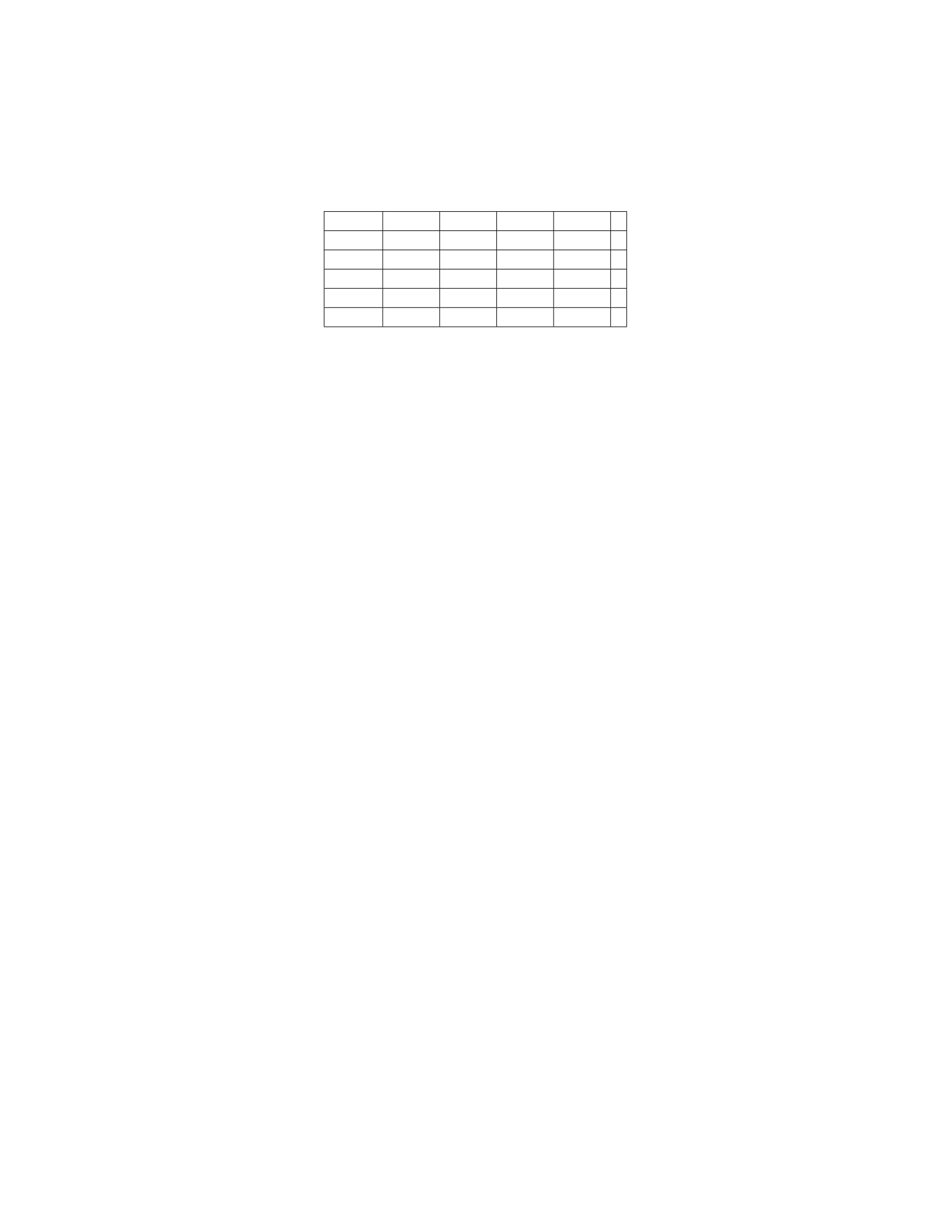
Y= 1 Y= 2 Y= 3 Y= 4
X= 1 0.05 0.10 0.05 0.10
X= 2 0.10 0.15 0.10 0.05
X= 3 0.20 0.15 0.05 0.00
X= 4 0.05 0.10 0.15 0.10
X= 5 0.00 0.00 0.10 0.15
Determine the least squares estimate of the regression coefficients β0and β1
in the simple linear regression model E(Y|X) = β0+β1X.
Solution
Step 1: Calculate the marginal probabilities of Xand Y.
The marginal probability mass function of Xis given by
pX(x) = ∑
y
pXY (x, y) = ∑
y
P(X=x, Y =y)
The marginal probability mass function of Yis given by
pY(y) = ∑
x
pXY (x, y) = ∑
x
P(X=x, Y =y)
Calculating these values gives: pX(1) = 0.30, pX(2) = 0.40, pX(3) =
0.40, pX(4) = 0.40, pX(5) = 0.25
pY(1) = 0.30, pY(2) = 0.35, pY(3) = 0.45, pY(4) = 0.40
Step 2: Calculate the sample means of Xand Y.
The sample means are given by
¯
X=
5
∑
i=1
xipX(xi),¯
Y=
4
∑
j=1
yjpY(yj)
Calculating these values gives: ¯
X= 3.45,¯
Y= 2.55
Step 3: Calculate the sample covariance and variance.
The sample covariance is given by
Cov(X, Y ) =
5
∑
i=1
4
∑
j=1
(xi−¯
X)(yj−¯
Y)pXY (xi, yj)
The sample variance is given by
Var(X) =
5
∑
i=1
(xi−¯
X)2pX(xi),Var(Y) =
4
∑
j=1
(yj−¯
Y)2pY(yj)
After calculating these values, we find: Cov(X, Y )=0.35,Var(X) =
1.2275,Var(Y) = 1.3475
21

Step 4: Calculate the least squares estimates.
The least squares estimates of the regression coefficients are given by
ˆ
β1=Cov(X, Y )
Var(X),ˆ
β0=¯
Y−ˆ
β1¯
X
Substitute the values we calculated above: ˆ
β1=0.35
1.2275 ≈0.2854,ˆ
β0= 2
Question 23
Question
Let y1, y2, y3, y4be a random sample from a normal distribution with unknown
mean µand unknown variance σ2. Consider the following estimator for µ:
ˆµ=1
4(y1+y2+y3+y4)
Show that ˆµis an unbiased estimator of µ.
Solution
Step 1: We need to show that E(ˆµ) = µ
Step 2: By linearity of expectation, we have:
E(ˆµ) = E(1
4(y1+y2+y3+y4))
Step 3: Since expectation is a linear operator, we can write this as:
1
4E(y1) + 1
4E(y2) + 1
4E(y3) + 1
4E(y4)
Step 4: Since y1, y2, y3, y4are from a normal distribution with mean µ, we
have E(yi) = µfor i= 1,2,3,4.
Step 5: Substituting this back into our expression, we get:
1
4(µ+µ+µ+µ) = µ
Step 6: Therefore, E(ˆµ) = µ, which means ˆµis an unbiased estimator of µ.
Question 24
Question
Suppose we have a dataset with the following values of independent variable x
and dependent variable y:
22

x1 2 3 4 5
y3 6 7 11 14
a) Find the least squares regression line that best fits the data.
b) Use the regression line to estimate the value of ywhen x= 6.
Solution
a) To find the least squares regression line, we need to calculate the slope and
intercept that minimize the sum of squared differences between the observed y
values and the predicted values from the regression line.
Step 1: Compute the means of xand yThe means of xand yare given
by:
¯x=1+2+3+4+5
5= 3
¯y=3+6+7+11+14
5= 8.2
Step 2: Calculate the slope of the regression line (b)The formula for
the slope of the least squares regression line is given by:
b=∑n
i=1(xi−¯x)(yi−¯y)
∑n
i=1(xi−¯x)2
where nis the number of data points. Calculating the numerator and denomi-
nator separately:
Numerator = (1 −3)(3 −8.2) + (2 −3)(6 −8.2) + (3 −3)(7 −8.2)
+ (4 −3)(11 −8.2) + (5 −3)(14 −8.2)
=−11.4
Denominator = (1 −3)2+ (2 −3)2+ (3 −3)2+ (4 −3)2+ (5 −3)2
= 10
Therefore, the slope bis given by:
b=−11.4
10 =−1.14
Step 3: Calculate the intercept of the regression line (a)The formula
for the intercept is:
a= ¯y−b¯x
Substitute the values of ¯y,b, and ¯xto find a:
a= 8.2−(−1.14 ×3) = 11.64
Hence, the least squares regression line is given by:
ˆy= 11.64 −1.14x
23

Question 25
Question
Let y=
−1
1
2
and X=
1 1
1 2
1 3
. Find the least squares estimate of βin the
model y=Xβ +ϵ, where ϵ=
1
−1
0
.
Solution
Step 1: Calculate the matrix product XTX.
XTX=(1 1 1
1 2 3)
1 1
1 2
1 3
=(3 6
6 14)
Step 2: Calculate the matrix product XTy.
XTy=(111
123)
−1
1
2
=(2
3)
Step 3: Solve the normal equations XTXˆ
β=XTyfor ˆ
β.
(3 6
6 14)ˆ
β=(2
3)
Step 4: Solve the system of equations to find ˆ
β.
{3ˆ
β1+ 6 ˆ
β2= 2
6ˆ
β1+ 14 ˆ
β2= 3
Solving these equations gives ˆ
β1=−1and ˆ
β2= 1/2.
Therefore, the least squares estimate of βis ˆ
β=(−1
1/2).
24

