BRIEF INTRODUCTION TO TREES

Binary search trees are a subclass of binary trees, which

are a subclass of trees, which are a subclass of graphs.

Here we will only introduce enough details to facilitate an

understanding of binary search trees. In chapter 11, we will

provide more precise mathematical definitions of graphs

and trees.

Trees (as well as graphs in general) consist of

nodes and edges. As a note, nodes are also referred to

as vertices (or vertex

in the singular form). We will use nodes as containers for

data, such as an integer, string, or even a database

record. Nodes are related to other nodes via edges. Each

edge connects two nodes and describes the relationship

between those nodes. Edges in binary trees are

child/parent relationships. One node is the parent, and the

other is a child. Each node has at most one parent. A tree

will have exactly one node without a parent. This node is

called the root. Each node has no more than two children.

A node with zero children is called a leaf. From time to

time, we may consider a subtree, which is any given node

and all its descendants. Although this chapter will focus

mainly on binary trees, you should note the term “m-ary

tree,” where m is any positive integer and represents the

maximum number of children for any given node.

Now we consider some additional tree-related

terms. It is important to note that these terms are not

consistently defined across different textbooks. In order to

be consistent with another source you may likely read

(Wikipedia), I will defer to the definitions found there.

Whenever reading a new text, ensure that you first review

that source’s definition of terms:

• height—the number of nodes from a leaf node to the

root, starting at 1

• depth—the number of nodes from the root to a

particular node, starting at 1

•

level—all descendants of the root that have the same depth

•

full—a given m-ary tree is full if each node has

exactly 0 or m children

•

complete—a given m-ary tree is complete if every

level is filled except possibly the last (which is filled

from left to right)

•

perfect—a given m-ary tree is perfect if it is full

and all leaf nodes are at the same depth

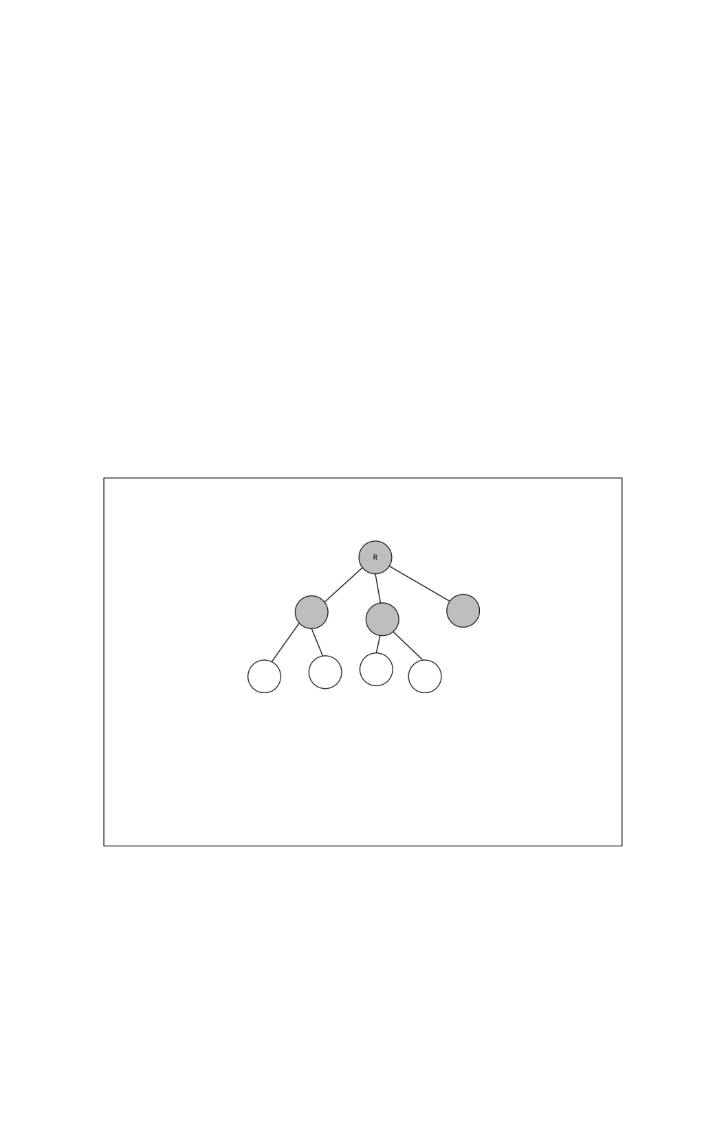
Below is an example of a tree. Interior nodes are gray, and

leaf nodes are white. The root node has been marked with

an “R.” Note that this is a ternary tree because any given

node has at most three children. It is not full, which

implies that it is neither complete nor perfect.

We may now make some useful assertions regarding binary

trees:

•

Because a perfect binary search tree implies that

every interior node has two children, the number of

nodes (n) is 2k − 1, where k is the number of levels in

the tree. In a related manner, the number of levels in a

Figure 8.1

tree is the floor of log

2

n.

•

Of all nodes in a perfect binary search tree, roughly

half are leaf nodes, and the other half are interior.

Precisely, the number of leaf nodes will be the

ceiling of n/2, and the number of interior nodes will

be the floor of n/2.

So far this concept of a tree does not produce

much benefit. We could assign a key to each node, but

what exactly would that mean? What does the relationship

between parent and child imply? To derive value from

trees, binary trees are insufficient, and we must apply

more constraints.

A binary search tree (BST) is a specific type of

binary tree that ensures that

•

each node (N) is assigned a key.

•

each node has a left child (L), which represents the

subtree

rooted at node L. The key of every node in this

subtree is less than the key stored in node N. It is

possible that a given node

has no left child.

•

each node has a right child (R), which represents the

subtree rooted at R. The key of every node in this

subtree is greater than the key in node N. It is

possible that a given node has no right child.

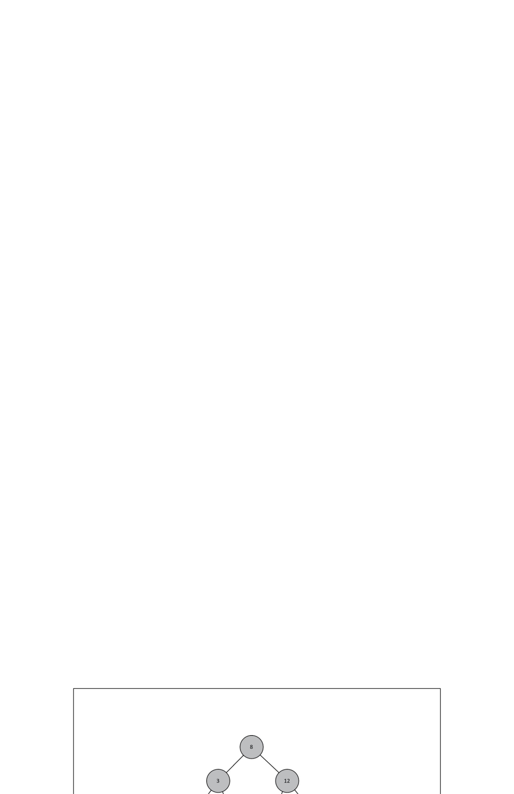
Figure 8.2 is an example of a BST. The key stored

in each node is an integer but could be of any data type

that can be sorted. For convenience, we are assuming that

BSTs do not contain duplicate keys, although we do not

exactly need to. The tree below is perfect, but a BST does

not need to be. As we discuss BSTs further, we will start to

consider more problematic configurations.

Figure 8.2

To understand the structure of a BST better, we can

Figure 8.2

consider an in-order traversal of the tree. This traversal is

one in which we recursively visit the left child, current

node, and right child. If you were to print each key during

an in-order traversal, the result would be all keys from the

tree in ascending order.

As implied in the figure above, nodes are modeled

using the following class. In most practical applications,

the Key property would hold some data other than type

integer. Regardless, the simplicity of this model will be

useful for the remainder of the chapter.

Searching

Searching is a simple operation. You begin at the root node

considering a key (x) you want to find. If the key stored at

the node is x, you have found it. If x is less than the node’s

key, you search the left subtree. If x is greater than the

node’s key, you search the right subtree. You continue this

process until you arrive at a leaf node and have no more

children to consider. Below is the pseudocode to further

clarify the algorithm. The function is originally called with

the root node, which then changes to descendants in the

recursive calls.

Next, we should consider the runtime of searching a BST.

Just as with searching arrays and linked lists, we want to

consider the amount of work necessary as the size of the data

structure increases. In our recursive example above, we

perform between 1 and 5 comparisons on each call to

search (depending on exactly how you count). As a result,

we have no more than 5 comparisons for each node visited.

Because 5 is not dependent on the overall number of nodes,

the amount of work to perform for each node visited is

constant with respect to n.

How many nodes must we visit in the worst-case

scenario? If we compare the desired value to the key at

the root node and do not find the value, we have

immediately eliminated roughly half of the values in our

tree. Once at the second level, we perform the comparison

again and eliminate half of this subtree, which was in turn

half of the original. As a result, we reduce the number of

keys we have to consider by half each time we visit a child.

At worst, we will have to visit only one node in each level

of the tree, resulting in ceiling log

2

n nodes visited. With

O(log n) nodes visited and O(1) amount of work at each

node, search can be run in O(log n) time for a perfect BST.

Insertion

To this point, we have assumed that a BST exists. We have

yet to create one. Insertion simply searches for a valid

position where the key would be if it existed and adds it at

that position. In other words, the search for a nonexistent

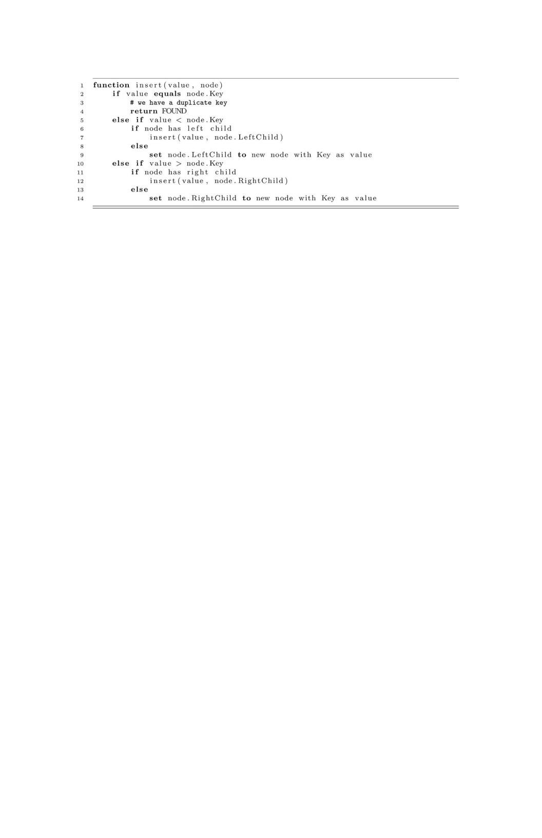
key always terminates in a leaf node. A naïve insertion

algorithm considers this leaf node. If the key to insert is

less than the leaf’s key, you insert a new node as the left

child. If the new key is greater than the leaf’s key, you

insert it as the right child. Pseudocode is included below to

clarify:

Deletion

When possible, it is good practice to enumerate the

possible states that an algorithm may have to consider.

When deleting a key from a BST, the node containing that

key may be in four different states with respect to its

children: no children, left child only, right child only, and

both left and right children.

No Children

First, we must locate the node containing the key to be

deleted. If that node has no children, it is by definition a

leaf node. To delete a key at the leaf node, it suffices to

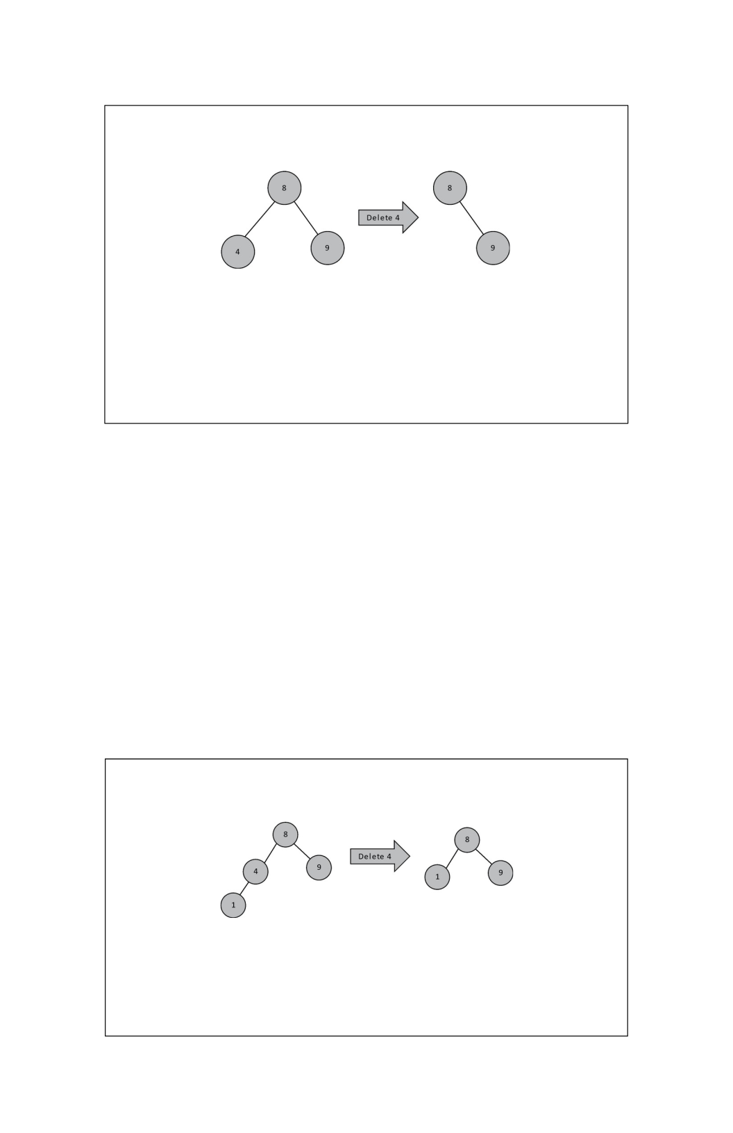
simply remove the parent’s reference to the leaf node. In

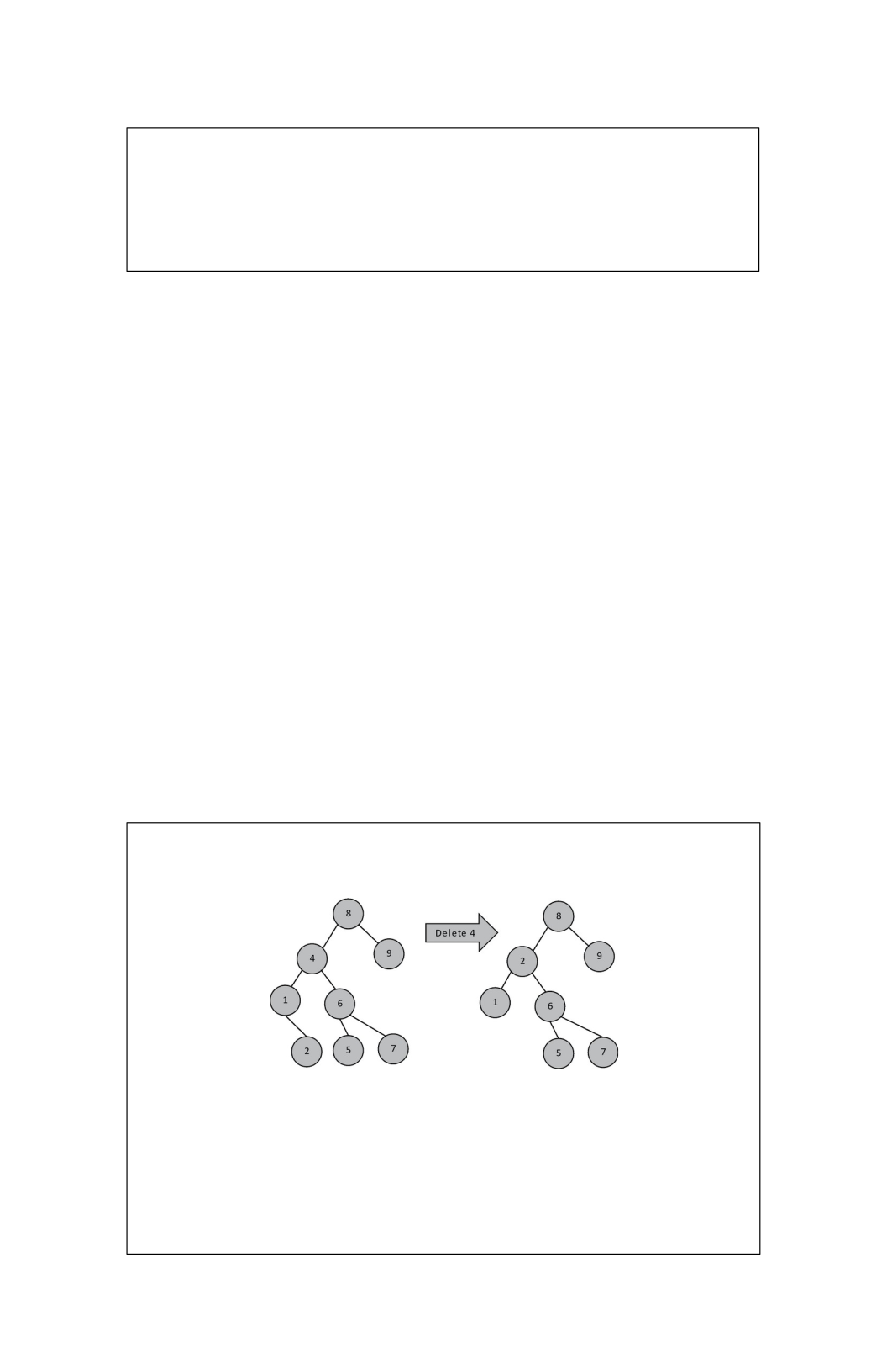
the example below, the node containing the value 4 has no

children. We can simply go to that node’s parent and set

the left child reference to null.

Left Child Only / Right Child Only

If a node contains a key to be deleted and has only

one child, we can shift the appropriate subtree up. We

can do this because all descendants in a node’s left

subtree are less than that node’s value. In the case below,

all left-side descendants of 8 are nodes containing values

less than 8. If 4 only has one child, we can simply promote

that child by setting 8’s left child to that node. Similar

reasoning would apply if 4 only had a right child.

Figure 8.3

Both Left and Right Children

If a node containing a value to be deleted has both left

and right children, we now must consider the possibility

that those children

may also be parents. This notably

complicates the decision of what should be node 8’s left

child. If we were to shift the subtree starting at 1 up to 8’s

left child, that new node would have two right children

(2

and 6), which obviously does not work. You would

encounter a similar issue trying to promote 6 to be 8’s

left child. What we need instead is to find 4’s in-order

predecessor or in-order successor, remove that value

from the tree (it is a leaf), and place it where 4

was. In

the example below, we promoted 4’s in-order predecessor,

but we could have just as easily promoted the value 5.

Figure 8.5

Figure 8.4

Unbalanced

BSTs

When assessing the performance of search in BSTs, we had

silently assumed that trees are perfect (or at least

complete). We relied on this convenient property that the

height of the tree was related to the logarithm of the

number of nodes. In practice, this is rarely the case. Imagine

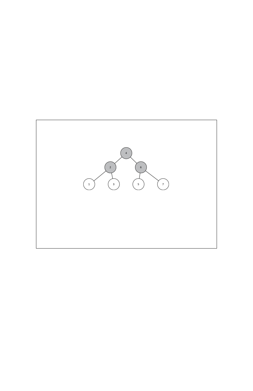
we built a perfect BST using keys 1 through 7.

In figure 8.6, we can visualize the relationship

between the number of nodes and the height of the tree. This

relationship is logarithmic, so we can count on searching,

inserting, and deleting keys to run in logarithmic time.

However, if we perform inserts as specified above (in order

from 1 to 7), we will actually end up with the tree in figure

8.7. Take a moment to trace the algorithm with

pencil and

paper to convince yourself this is the case.

Figure 8.6

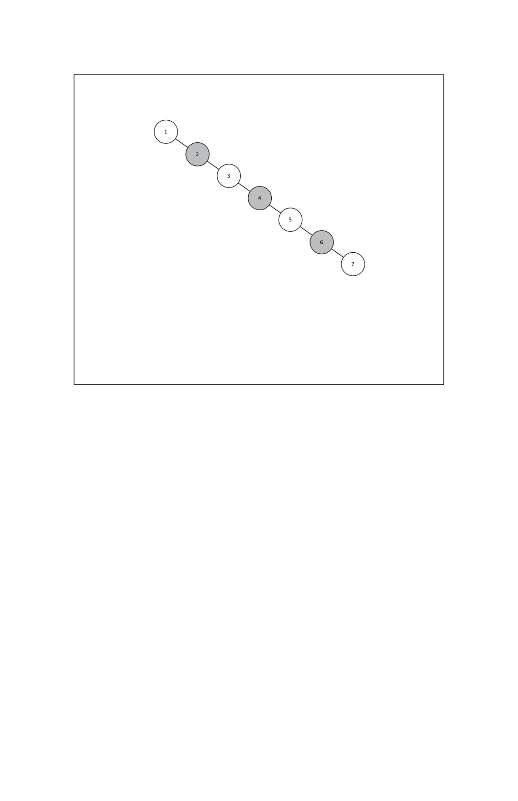
Our resulting structure, although technically a BST,

also closely resembles a sorted linked list. When we

studied linked lists, we were only able to search in linear

time because all n nodes must be visited to ensure we

found the desired key. The lesson learned is this: if we

are not careful about how we perform inserts, we may

likely construct a tree structure that cannot support O(log

n) searches.

Ideally, we would love a tree to be perfect after

each insert. This is not mathematically possible. If you

have a perfect tree with seven nodes and three levels,

inserting an eighth node will create a new level and result

in a state where not all leaf nodes have the same depth. It

may be desirable to maintain a complete tree. However,

recall that complete trees must fill the lowest level from

left to right. This constraint is not necessary, as we will be

just as happy to fill it out right to left or in completely

arbitrary order. As we can see, we need a new term to

describe BSTs that allow for O(log n) searches and avoid

the linked list type of configuration.

Figure 8.7

In a manner of speaking, we want our tree to be

balanced after each insert. At this time, we will loosely

define balance to be the condition such that the subtree

heights of left and right subtrees are roughly equal. That

leads to our next question: Can we modify our insert such

that (1) the tree can remain balanced after each insert and

(2) inserts can still be performed in O(log n) time?

Self-Balancing

Trees

Self-balancing trees are those that maintain a balanced

structure after each insertion and deletion and thus

maintain an O(log n) search time. A thorough survey of

these data structures could constitute chapters of text.

This section will introduce how AVL trees maintain a

balanced structure during insertion. We focus only on the

insertion, but deletion must be addressed as well. Search,

however, does not change from the naïve BST. Additional

resources at the end of the chapter provide more

information about this and other self-balancing trees.

AVL Trees

AVL trees are named after the computer scientists who

developed them (G. M. Adelson-Velsky and E. M. Landis).

After insertions that leave the tree in an unbalanced state,

we achieve balance by performing small constant-timed

adjustments called rotations.

First, we must determine whether an insertion has

resulted in an unbalanced tree. To determine this, we use

a metric called the balance factor. This integer is the

difference in the heights of a node’s left and right

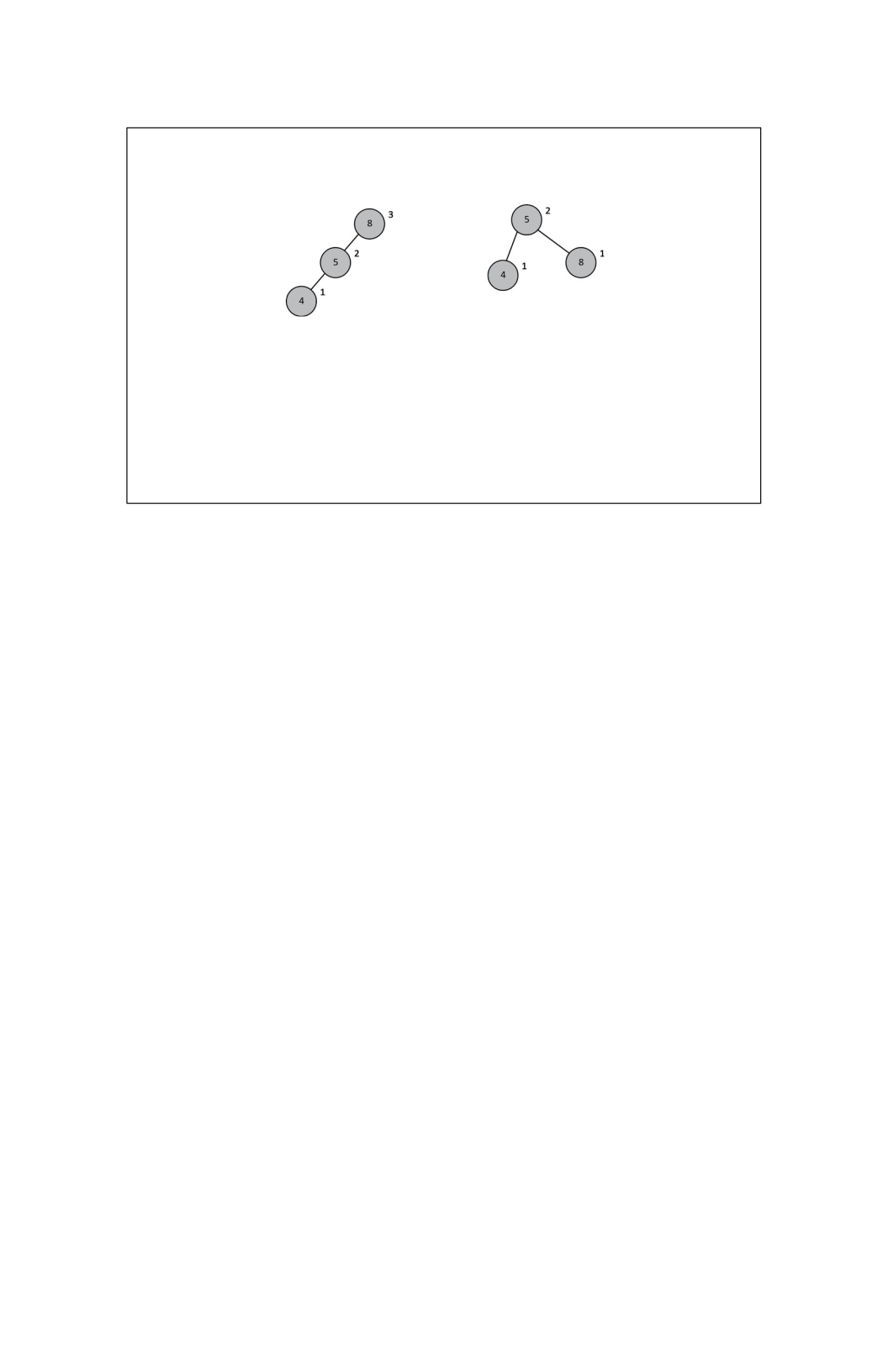
subtrees. Below is the simplest possible tree where we can

witness such an imbalance. As usual, values are stored

inside the node. Subtree heights are stored at the upper

right of

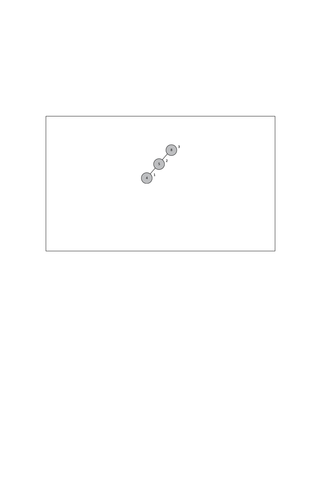
each node. If a left or right child does not exist, then the

subtree height is 0. In this example, the node containing 8

has a left child with subtree height of 2 and a right child

with subtree height of

0. The absolute difference between 2 and 0 is 2. This is

above our threshold of 1, so our tree is unbalanced.

We now have a means for detecting unbalanced

trees and are left to determine how to bring the tree back

into balance. This is where we employ rotations. Rotations

are small, constant-time adjustments to a subtree that

improve the balance of that subtree. They are called

rotations because they have the visual effect of rotating

that subtree to a more balanced state. In figure 8.8, a

rotation makes the 5 node the new root with a left child

of 4 and a right child of 8. This is visually depicted in figure

8.9. Notice that after the rotation, the height of the subtree

starting at 8 is now 1. Node 5 has left and right subtrees

both at height 1. The difference is 0, which is not greater

than 1, indicating that we are now in balance.

Figure 8.8

We make one last consideration regarding AVL

trees. Earlier we had described this modification to BSTs as

“self- balancing” and the heights of left and right subtrees

as roughly equal. What actually happens is more nuanced

and worthy of discussion. With perfect BSTs, we concluded

that the relationship between the number of nodes in the

tree and the number of comparisons required for a search

was logarithmic. For AVL trees, we must be able to show

the same relationship applies.

A proof by induction is able to show that the height

of any AVL tree is O(log n). Note the distinction here.

Perfect binary trees were shown to have a height equal to

the ceiling of log

2

n (or more precisely, log

2

(n+1)). AVL

trees are said to have a height of O(log n), which is less

precise. Rather than reviewing the inductive proof (which

can easily be found online and in many reference

textbooks), let us consider the following two trees:

Figure 8.9

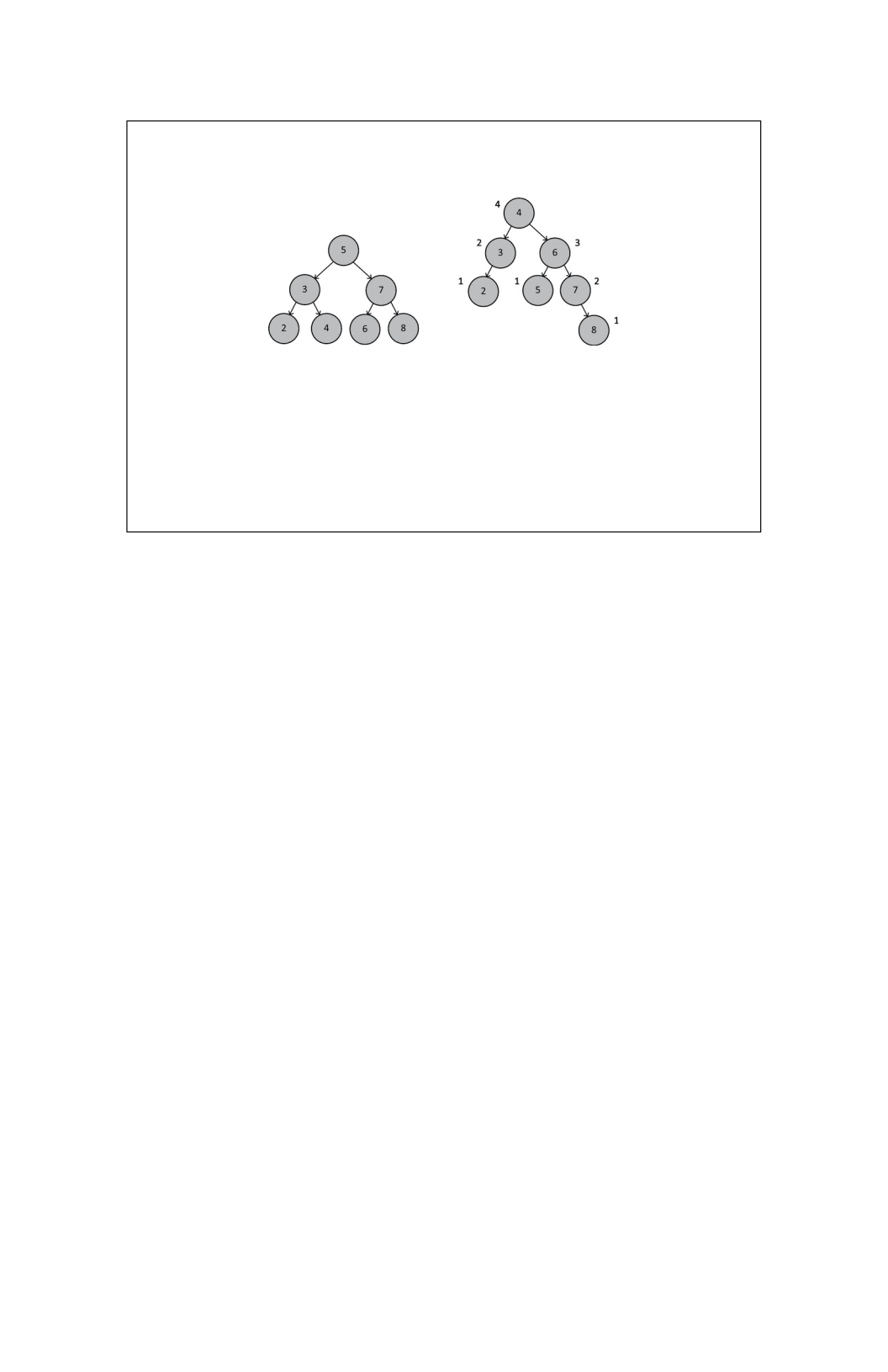
The tree on the left is a perfect BST. It has 7 nodes,

which implies a height of log2(7+1) = 3. The tree on the right

is a balanced AVL tree. Note that the height is no longer 3,

even though we claim that the tree is balanced and that

search times are still O(log n). We point this out to illustrate

that while some algorithms may share the same Big-O

classification, their actual runtimes may differ. Because of

the rotations, we ensure that the difference in heights of

the left and right subtrees is no more than 1. This then

ensures that our AVL tree, while not complete or perfect, has

a height no greater than 1 + log2(n+1). The additional 1

does not significantly impact the growth of the function as n

becomes very large, so we can conclude that searching an

AVL tree can still be accomplished in O(log n) time.

Heaps

A heap is a data structure that guarantees that the

minimum (or maximum) value is easily extracted. The

most common heap is a binary heap, which is a sort of

Figure 8.10

binary tree. In a binary heap, the

“left” or “right” position of

a child node no longer carries any specific

meaning. Rather,

in a max-binary-heap, or just max-heap, the parent is

guaranteed to be greater than both children. Min-binary-

heaps naturally reverse that relationship, with the parent

guaranteed to be less than the children. We call this

quality the heap property. It will allow us to isolate our

reasoning to only subheaps and thus aid our

understanding of heap-related algorithms.

For the remainder of this section, we assume max-

binary- heaps to avoid confusion. We will also assume

unique values in our binary heap. This simplifies the

relationships between parents and their children. If a

particular application of binary heaps

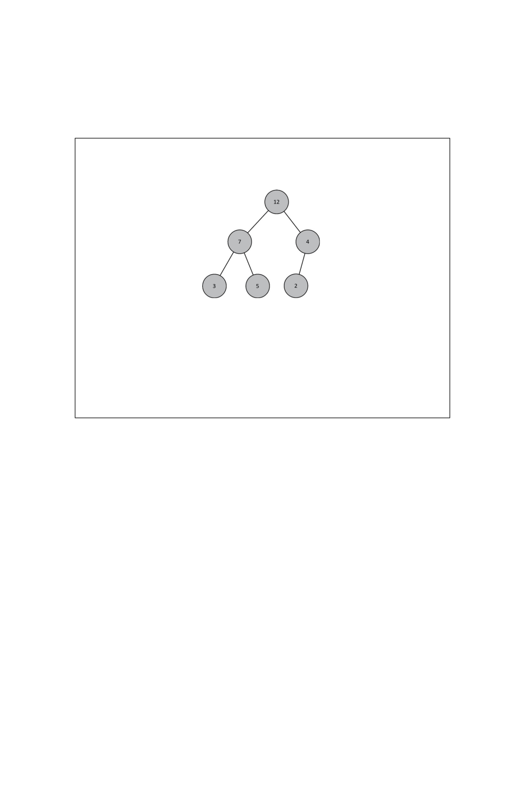
necessitates duplicate keys, this is easily remedied by

adjusting the appropriate comparisons. The figure below

gives an example of a heap:

This distinction between parent and child nodes

leads to two convenient properties of binary heaps:

•

For a given heap, the maximum value (or key) is

easily accessible at the root of the tree. As we will

soon see, this implies not that it is easily extracted

from the structure but simply that finding it is

trivial.

•

For any given node in a binary heap, all descendants

contain values less than that node’s value. In other

words, any given subtree of a max-binary-heap is also

a valid max-binary-heap.

Let us emphasize and further address a common

point of confusion. Although binary heaps are binary tree

structures, their similarities with binary search trees (BST)

end there. Recall from chapter 8 that an in-order traversal

of a binary search tree will produce a sorted result. This is

Figure 9.1

true because, for any given node

in a BST, all left descendants are less than that node, and

all right descendants are greater than it. In binary heaps,

the left descendant is less than the parent, and the right

descendant is less than it as well, but there is no other

defined relationship between the two descendants.

To understand insertion and extraction, first note

the shape of the binary tree above. A tree is a complete

binary tree if each node has two children and all levels are

filled except possibly the last, which is filled from left to

right (chapter 8). Using some clever tricks, we can store a

complete binary tree as an array. Because each level of

the tree is filled and the last is filled left to right, we

can simply list all elements in level 0, followed by all

elements in level 1, and so on. Once these values are

stored in an array, some simple arithmetic on the indexes

allows traversal from a node to its parents or its children.

We will be regularly adding and removing data from the

heap itself. As we have seen in prior chapters, arrays are

an insufficient data structure for accomplishing this. For

the sake of simplicity, we will assume excess capacity at

the end of the array. In practice, we would probably

use some sort of abstract list that is able to grow or shrink

and provides constant-time lookups. This might be

something like an array that automatically reallocates

when its capacity is reached. Implementations of these

lists exist in most modern languages. For the present

discussion, we can just treat the underlying storage as a

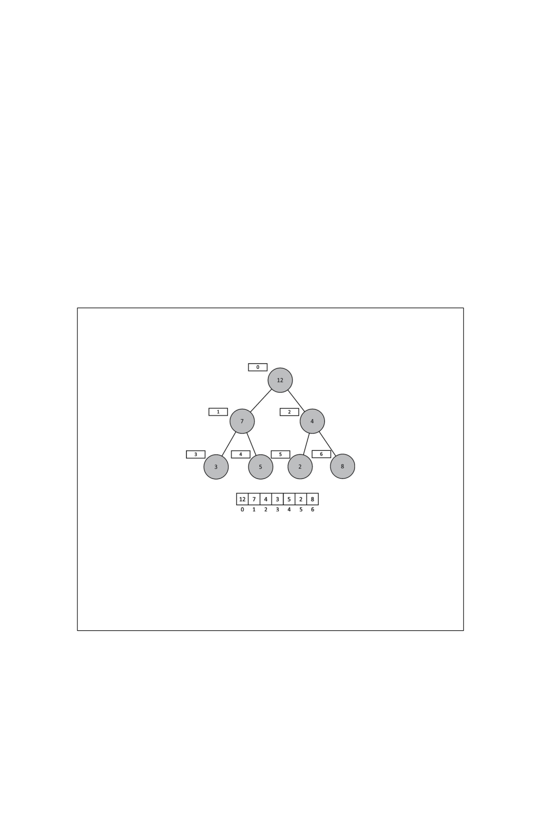
typical array. The image below shows a heap represented

as an array with integer values for the priorities:

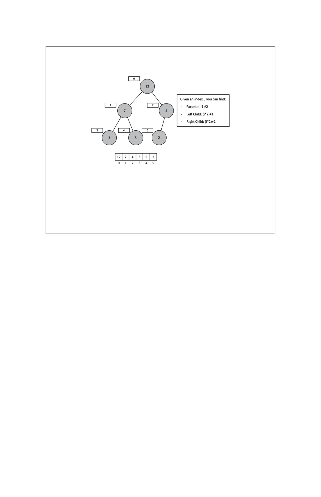
For now, we will work only with integers that

serve as the priorities themselves. To extend this into a

more useful data structure, we would need only to change

the contents of the array to an object or object reference.

This would allow us to hold a more useful structure such as

a student record or a game player’s data. Then the only

other change needed would be to do comparisons on

array[index].priority instead of just array[index]. This

modification is like the one we discussed regarding

Linear Search in chapter

4. Recognize that we can generalize this representation

easily to accommodate data records that are slightly more

sophisticated than just integers.

Operations

on

Binary

Heaps

Before we discuss the general operations on binary

heaps, let’s discuss some helper functions that will help

Figure 9.2

us with our array

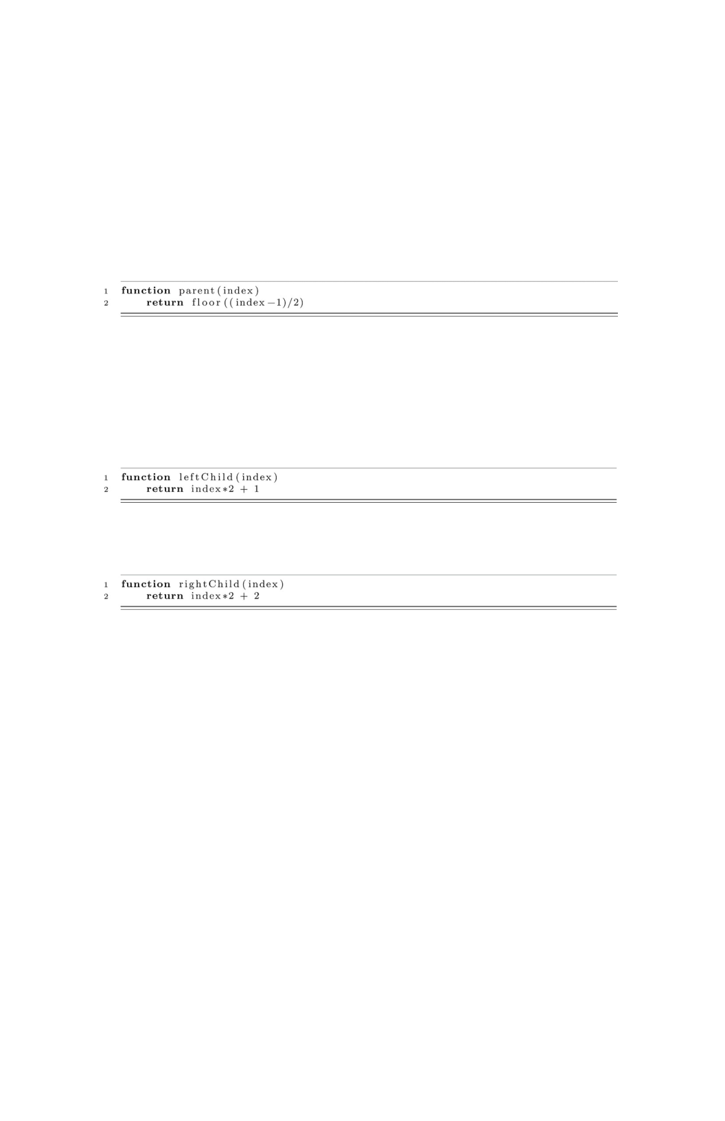
representation. We will define functions that will allow us

to find the parent, left child, and right child indexes given

the index for any node in the tree structure. These would

be helpful to define for any tree structure that we wanted

to implement using an array. For this representation, the

root will always be at the index 0. These are given in the

figure above, but we will provide them as code here:

Here the floor function is the same as the

mathematical function floor. It rounds down to the next

integer.

Heapify and Sift Up

Using the above functions to access positions in our tree,

we can develop two important helper functions that will

allow us to modify the tree and work to maintain our heap

properties. These are the functions heapify and siftUp.

When we are building our heap or modifying the priority of

an item, these functions will be useful. The heapify

function will exchange a parent with the larger of its

children and then recursively heapify the subheap. The

siftUp function will exchange a child with its parent to

maintain the heap property by moving larger elements up

the heap until it either is smaller than its parent or

becomes the root node element. The siftUp function will be

used when we want to increase the priority

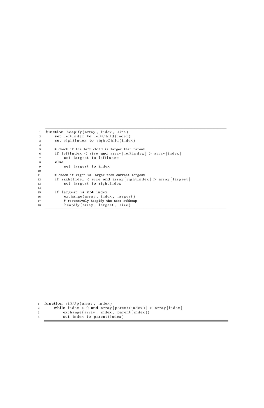
of an element. Let’s look at the pseudocode for these

functions in the context of an array-based max-heap

implementation.

The heapify function below lets a potentially small

value work its way down the max-heap to find its correct

place in the heap ordering of the tree. This code uses a

size parameter that gives the current number of elements

in the heap. This code also makes use of an exchange

function like the one discussed in chapter 3 on sorting. This

simply switches the elements of an array using indexes.

Now we will present the siftUp function. This

function works in the reverse direction from heapify. It

allows for a node with a potentially large value to make its

way up the heap to the correct position to preserve the

heap property. Since siftUp moves items toward index 0,

the size is not needed. This does assume that the given

index is valid.

With these two helper functions, we can now

implement the methods to insert elements and remove the

max-element from our priority queue. Before we move on

though, let’s think about the complexity of these

operations. Each of these methods moves items

up or down the depths of a binary tree. If the tree could

remain balanced, then a traversal from the top to bottom

or bottom to top should only require O(log n) operations,

assuming that the tree is balanced.

Insertion

Consider inserting the number 8 into the prior binary heap

example. Imagine if we simply added that 8 in the array

after the 2 (in position 6).

What can we now claim about the state of our

binary heap? Subheaps starting at indexes 1, 3, 4, and 5

are all still valid subheaps because the heap property is

preserved. In other words, our erroneous insertion of 8

under 4 does not alter the descendants of these 4

nodes. As a result, we could hypothetically leave these

Figure 9.3

subheaps unaltered in our corrected heap. This leaves

nodes at indexes 0 and 2. These are the two nodes that

have had their descendants altered. The heap property

between node indexes 2 and 6 no longer holds, so let us

start there. If we were to switch the 4 and 8, we would

restore the heap property between those two indexes. We

also know that moving 8 into index 2 will not affect the

heap property between indexes 2 and 5. If 2 was less than

4 and 4 was found to be less than 8, switching the 4 and 8

does not impact the heap property between indexes 2

and 5. Once the 4 and 8 are in the correct positions, we

know that the subheap starting at index 2 is correct. From

here, we simply perform the same operations on

subsequent parents until the next parent’s value is greater

than the value we are trying to insert. Given that we are

inserting 8 and our root node’s value is 12, we can stop

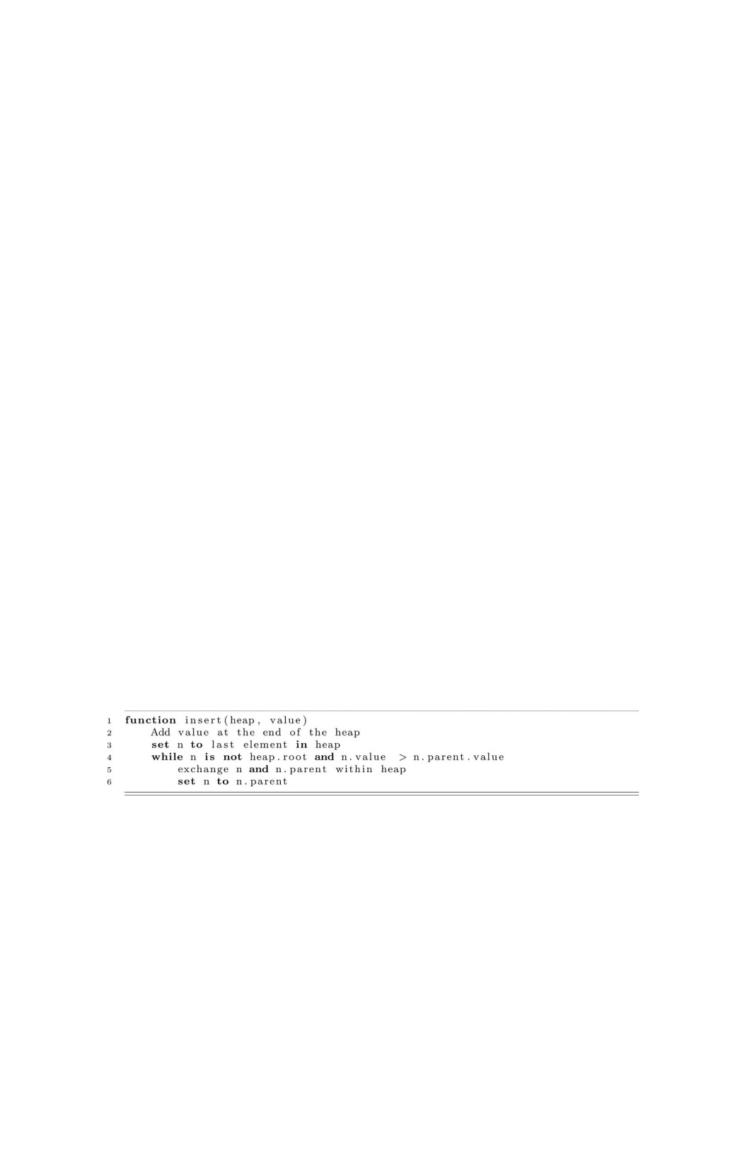
iterating at this point. The pseudocode below is descriptive

but much simpler than practical implementations, which

must consider precise data structures for storing the heap.

This provides the general pattern for inserting into a

binary heap regardless of the underlying implementation.

We place the new element at the end of the heap and then

essentially siftUp that element to the place that will

preserve the heap property.

Runtime of insertion is independent of whether the

heap is stored as object references or an array. In either

case, we have to compare n.value to n.parent.value at

most O(log n) times. Note that, unlike the caveat included

in binary search trees (where traversing an unbalanced

tree may be as slow as O(n)), binary heaps maintain their

balance by building each new depth level before increasing

its depth. This ensures that an imbalanced binary heap

does not occur. This fact guarantees that our insert

operation is O(log n).

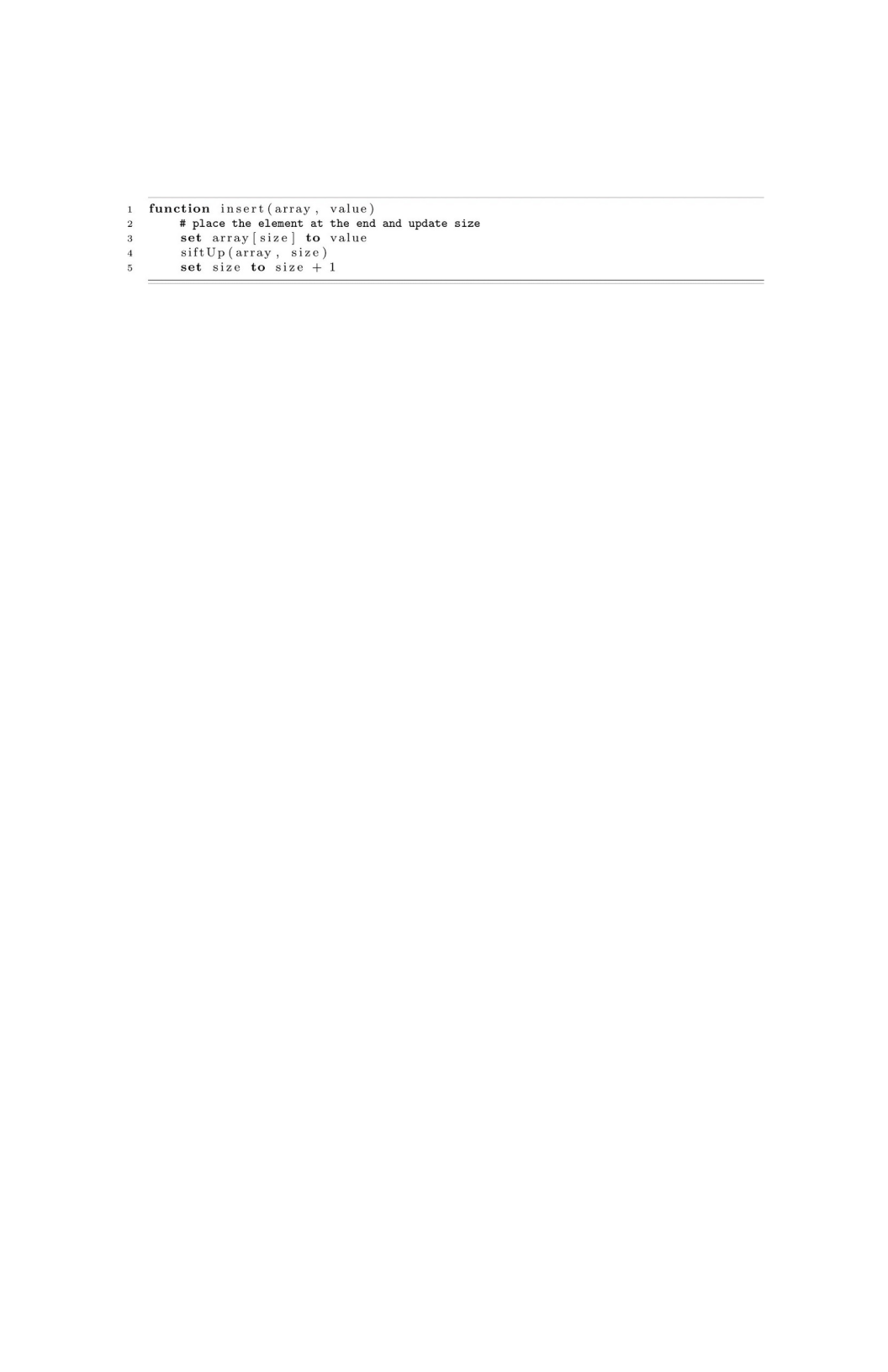
A specific implementation for insert with our array-

based heap is provided below:

Extraction

Extraction is the process of removing the root node of a

binary heap. It works much the same way as insertion but

in reverse. The general strategy is as follows.

To extract an element from the heap…

1.

Extract the root element, and prepare to return it.

2.

Replace the root with the last element in the heap.

3.

Call heapify on the new root to correct any

violations of the heap property.

As an example, consider our corrected heap from

before. If we overwrite our 12 (at index 0) with the last value

from the array (4 at index 6), the result will be as follows in

figure 9.5. Just as we saw with insertion, many of our

subheaps still have the heap property preserved. In fact, the

only two places where the heap property no longer holds

are from indexes 0 to 1 and 0 to 2. If the value at the

root is less than the maximum value of its two children,

then we swap the root value and that maximum. We will

continue this process of pushing the root value down until the

current node is greater than both children, thus conforming

to the heap property. In this case, we swap the 4 with the

8. The root node conforms to the heap property because its

children are 7 and 4. The node with value 4 (now at index 2)

only has one child (2 at index 5). It conforms to the heap

property, and our extraction is complete.

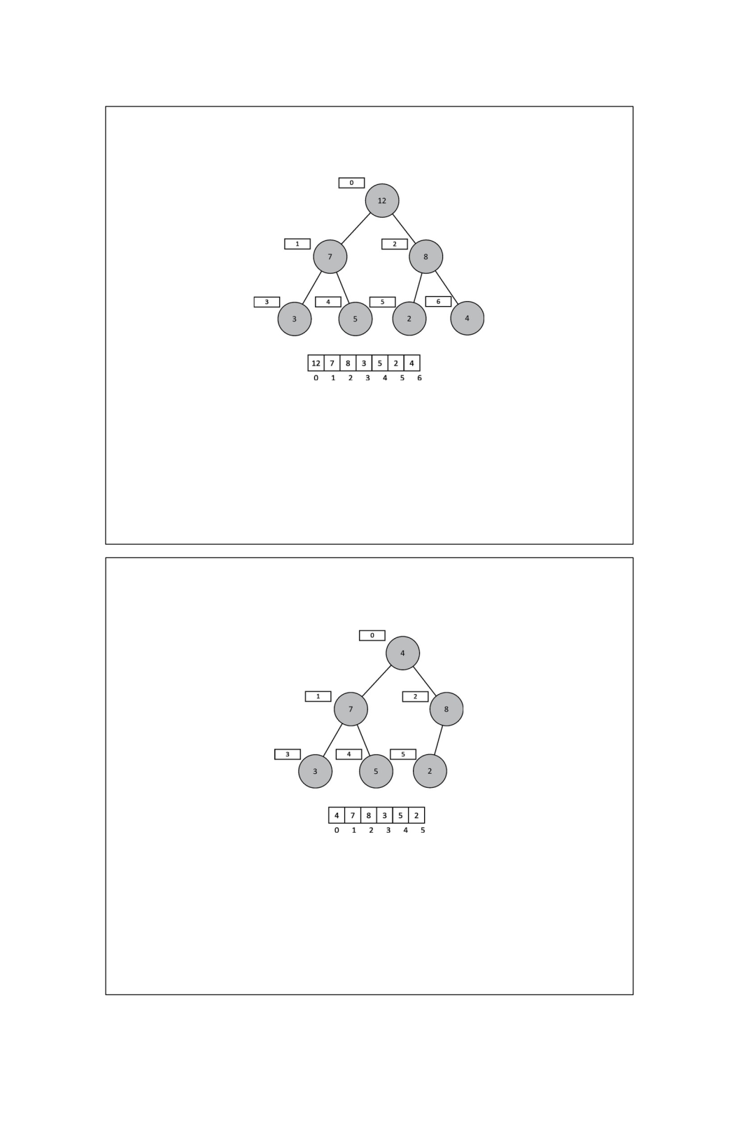
Figure 9.4

Figure 9.5

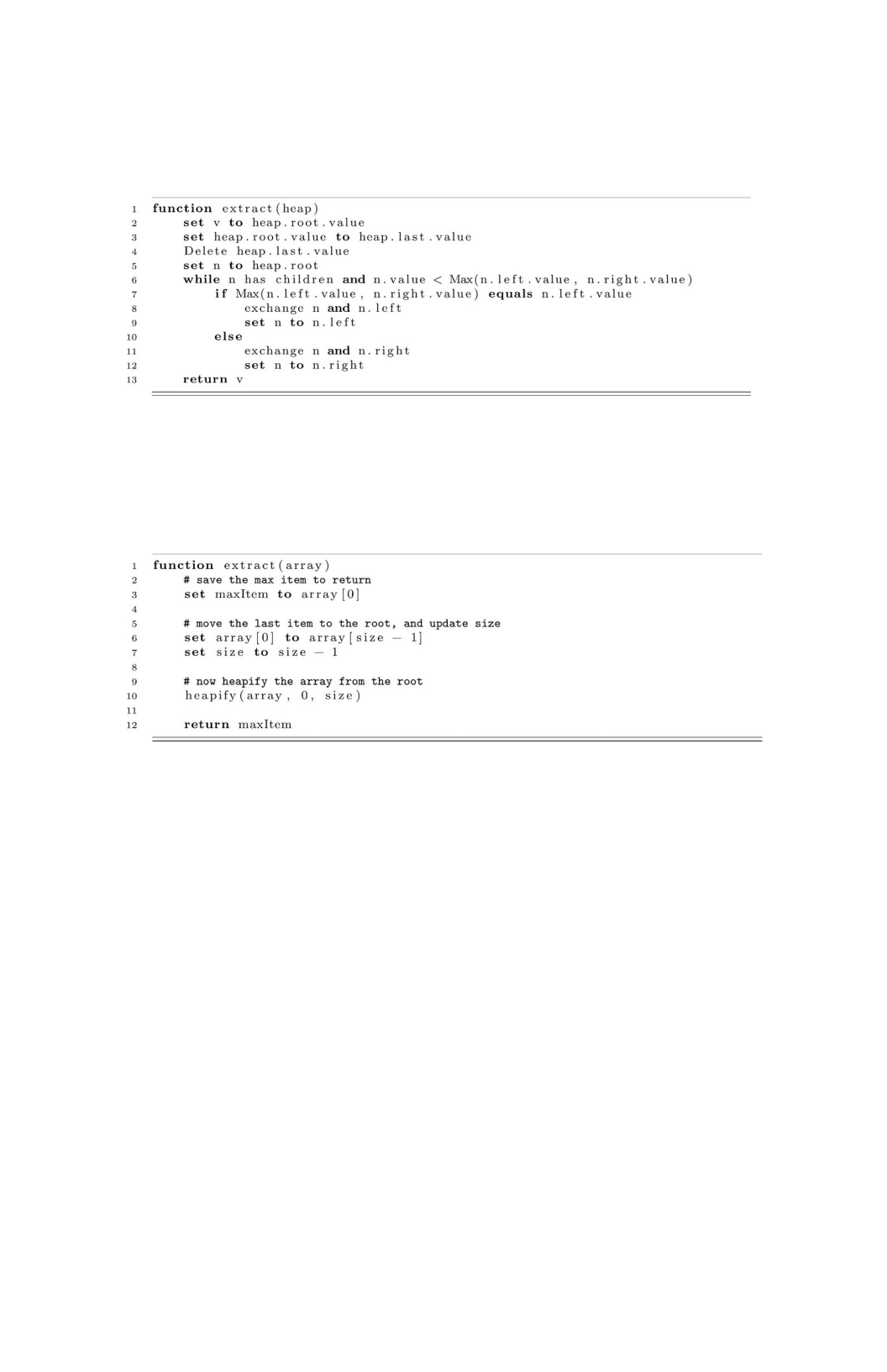
As before, the pseudocode is much simpler than

the actual implementation.

The array-based implementation could use the

heapify function to give the following code:

While accessing the max-element would only

require O(1) time, updating the heap after it is removed

requires a call to heapify. This function requires O(log n).

While not constant time, O(log n) is a great improvement

over our initial naïve implementation ideas from the

introduction. Our initial idea of sorting and then always

copying moving elements up or down would have required

O(n) operations to maintain our priority queue when

inserting and removing elements. The max-heap greatly

improves on these complexity estimates, giving O(log n)

for both insert and extract.

Heap

Sort

Heap Sort presents an interesting use of a priority queue.

It can be used to sort the elements of an array. Once

insertion and extraction have been defined, Heap Sort

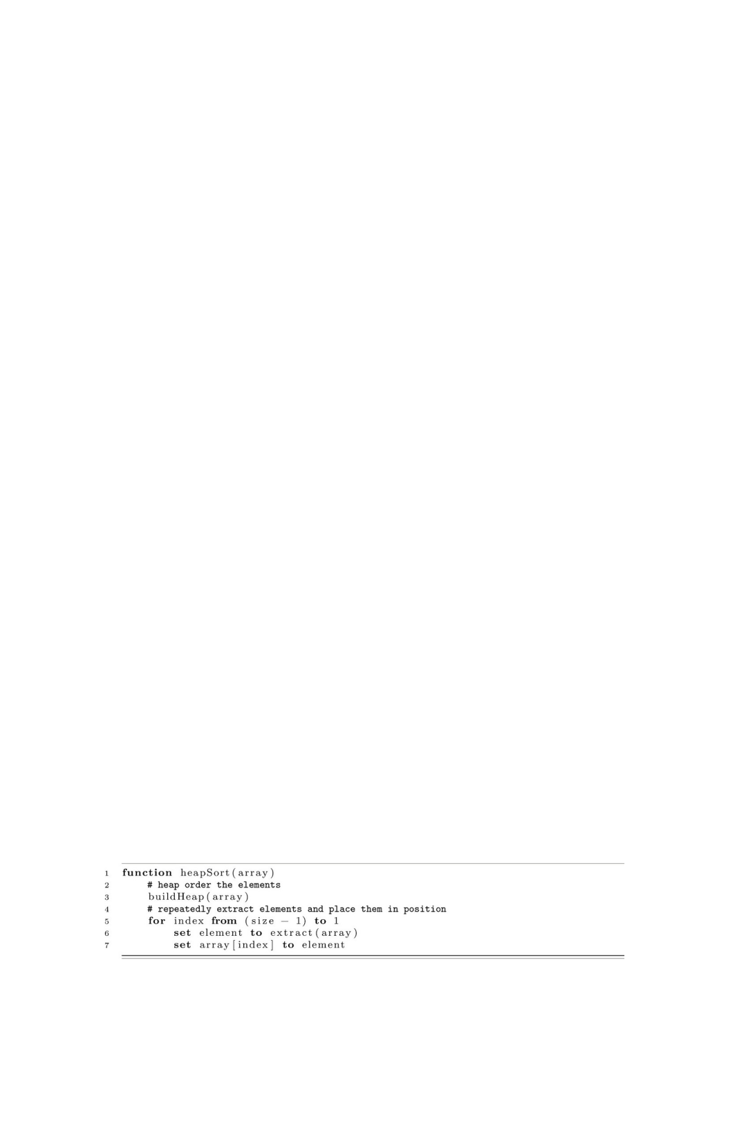
becomes a trivial step. We first build the heap, then

repeatedly extract the maximum element and put it at the

end of the array. Much like Selection Sort, Heap Sort will

find the extreme value, place it into the correct position,

then find the extreme of the remaining values. The trick is

in how we perceive the heap. If we model it using an array,

we can then sort the values in place by extracting the

maximum. The extraction makes the heap smaller by one,

but arrays are fixed size and still have the extra space

allocated at the end. This portion at the end of the array

becomes our sorted portion. As we perform more

extractions and move those extracted values to the end of

the array, our sorted portion gets bigger. See the figure

below for an example. Unlike Selection Sort, where finding

that extreme value requires an O(n) findMax or findMin,

heaps allow us to extract the extreme value and revise our

heap in O(log n) time. We perform this operation O(n)

times, resulting in an O(n log n) sorting algorithm. The

following figure gives an example execution of the sorting

algorithm:

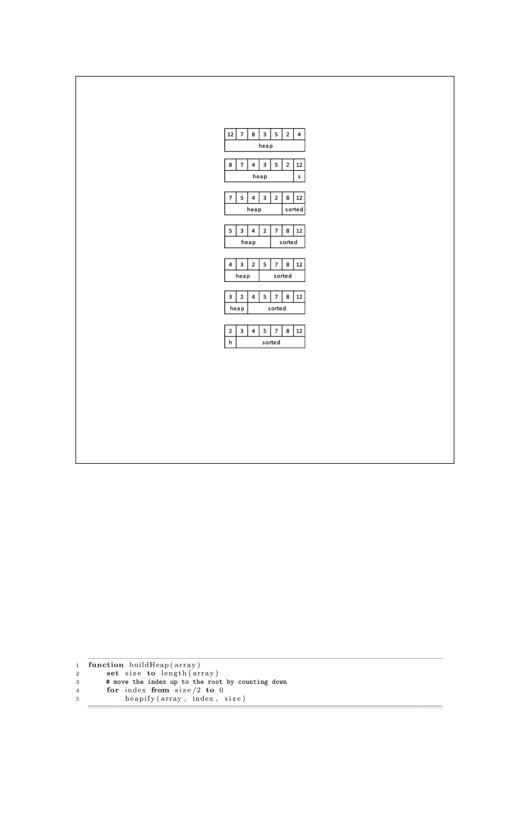
Before we give the implementation of Heap Sort,

we should also mention how to build the heap in the first

place. If we are given an array of random values, there is

no guarantee that these will conform to our requirements

of a heap. This is accomplished by calling the heapify

function repeatedly to build valid heaps starting at the

deeper levels of the balanced tree up to the root. Below

is the code for buildHeap, which will take an array of

elements to be sorted and put them into the correct heap

ordering:

Figure 9.6

It might be unintuitive, but buildHeap is O(n) in its

time complexity. At first glance, we see heapify, an O(log

n) operation, getting called inside a loop that runs from

size/2 down to 0. This might seem like O(n log n). What we

need to remember though is that O(log n) is a worst-case

scenario for heapify. It may be more efficient. As we build

the heap up, we start at position size/2. This is because

half of the heap’s elements will be leaves of the binary tree

located at the deepest level. As we heapify the level just

before the leaves, we only need to consider three

elements: the parent and its two leaf children. As heapify

runs, the amount of work is proportional to the height of

the subtree it is operating on. Only on the very last call

does heapify potentially visit all log n of the levels of the

tree. We will omit the calculation details, but it has been

proven that O(n) gives a tighter bound on the worst-case

time complexity of buildHeap.

Now we are ready to implement Heap Sort. An

implementation is provided below. Our O(n log n)

complexity comes from calling heapify from the root every

time we extract the next largest value. Another useful

feature of this algorithm is that it is an in-place sorting

algorithm. This means the extra space (auxiliary space)

only consumes O(1) space in memory. So Heap Sort

compares favorably to Quick Sort with a better worst-case

complexity (O(n log n) vs. O(n

2

)), and it offers an

improvement over Merge Sort in terms of its auxiliary

space usage (O(1) auxiliary space vs. O(n)). We should

note that Heap Sort may perform poorly in practice due to

cache misses, since traversing a tree skips around the

elements of the array.

This section has provided an overview of heapSort and the

concept of a heap more generally. Heaps are great data

structures for implementing priority queues. They can be

implemented using arrays or linked data structures. The

array implementation also demonstrates an interesting

example of embedding a tree structure into a linear array.

The power and simplicity of heaps make them a popular

data structure. One potential disadvantage of the heap is

that merging two heaps might require O(n) operation. To

combine these two heaps, we would need to create a new

array, recopy the elements, and then call buildHeap, taking

O(n) operations. In the next section, we will discuss a new

data structure that supports an O(log n) union operation.

Binomial

Heaps

The binomial heap supports a fast union operation. When

two heaps are given, union can combine them into a new

heap containing all the combined elements from the two

heaps. Binomial heaps are linked data structures, but they

are a bit more complex than linked lists or binary trees.

There is an interesting characteristic to their structure,

which models the pattern of binary numbers, and

combining them parallels binary addition. Binary numbers

and powers of 2 seem to pop up everywhere in computer

science. In this section, we will present the binomial heap

and demonstrate how it can provide a fast union operation.

Then we will see how many of the other operations on

heaps can be implemented with clever use of the union

function.

Linked

Structures

of

Binomial

Heaps

To build our heap, we need to discuss two main structures.

The first part is the binomial tree. Each binomial tree is

composed of

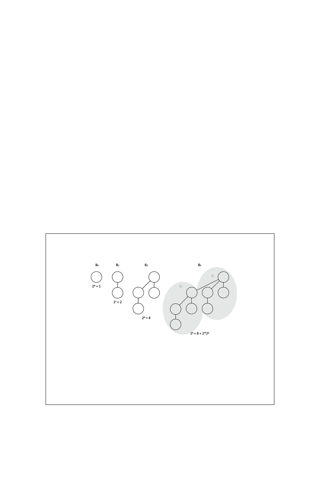
connected binomial nodes. The structure of a binomial

tree can be described recursively. Each binomial tree has

a value k that represents its degree. The degree 0 tree,

B

0

, has one element and no children. A degree k tree, Bk,

has k direct children but 2k nodes in total. When the Bk

tree is constructed, the roots of two Bk−1 trees are

examined. The largest root of the two trees is assigned as

the root of the new tree, assuming a max-binomial-heap.

The heap is then represented as a list of binomial trees.

A collection of trees is known as a forest. The main idea of

the binomial is that each heap is a list of trees, and to

combine the two heaps, one just needs to combine all the

trees of equal degree. To facilitate this, the trees are

always ordered by increasing tree degrees. A few

illustrations will help you understand this process a little

better.

Using these trees, a heap would then be a list of

these trees. To preserve the max-heap property, any

node’s priority must be larger than its child. Below is an

example binomial heap. Let’s call this heapA:

Figure 9.7

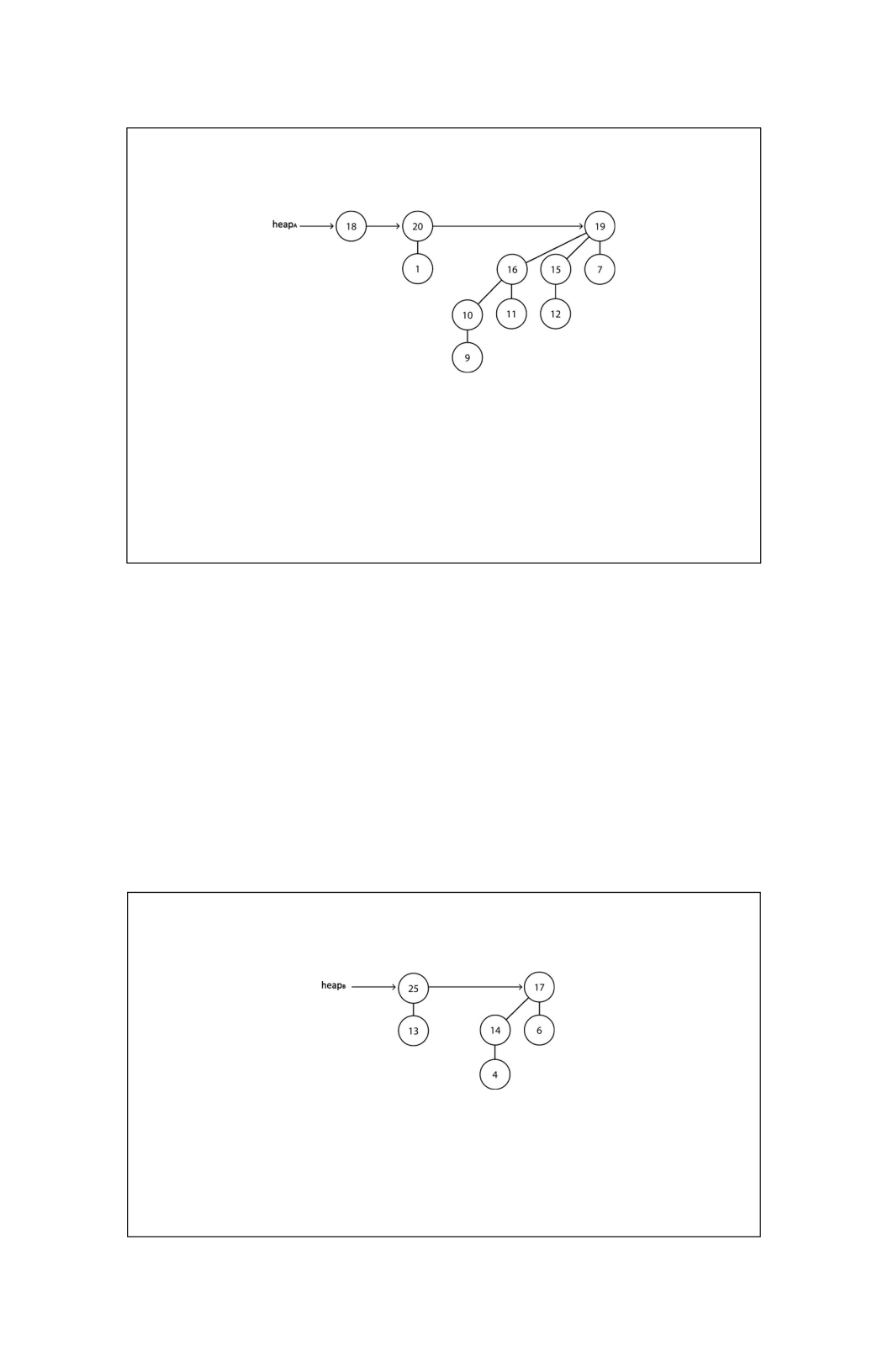
Notice that the maximum element is in B1 tree of this

heap. This illustrates that the actual max-heap element is one

of the root nodes of trees in the list. Now we can make the

connection to binary numbers. This heap will either have a

tree of any given degree or not. This could be indicated by a

0 or 1. So the above heap has a degree 0 tree, a degree 1

tree, and a degree 3 tree. In binary with the bits correctly

ordered, this would be 10112 or the number 1110 in base

10. Suppose there is another heap, heapB, that we wish to

merge with. This is given below:

Figure 9.8

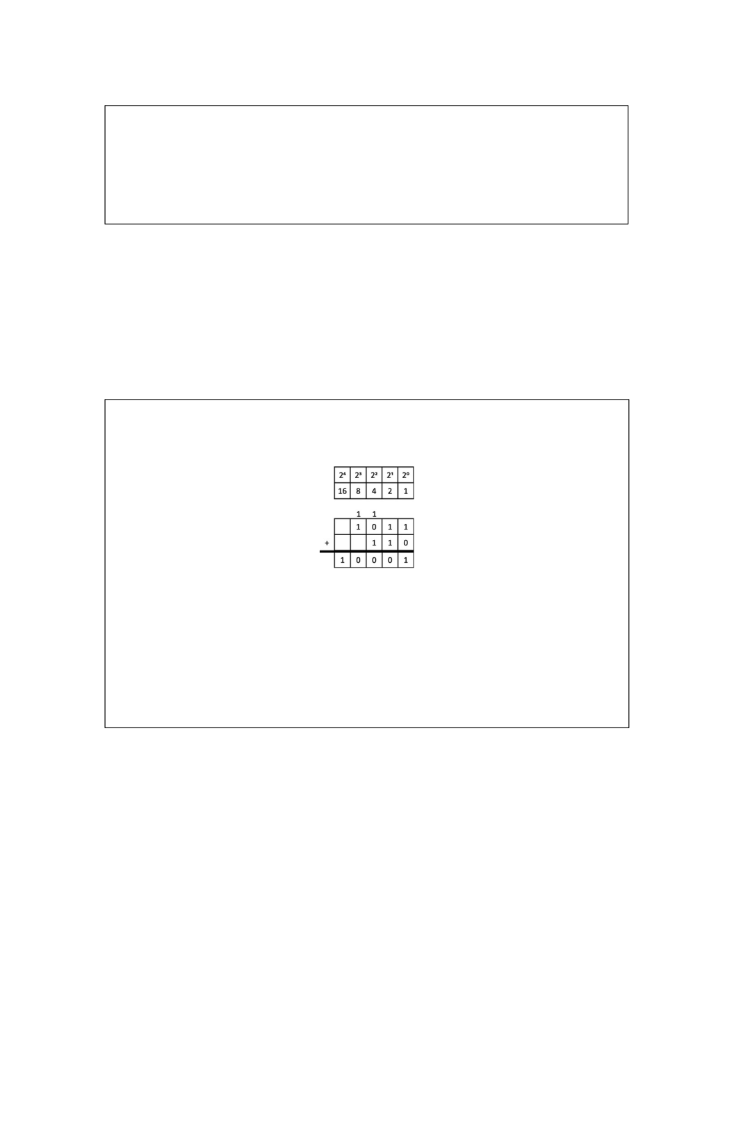
This heap has trees for degrees

1

and 2. In binary,

we could represent this pattern as 1102 or the number

610 in base 10. We will soon look at how these heaps

could be merged, but first let’s consider the process of

binary addition for these two binary numbers:

11

and 6.

The figure below gives an example of the addition:

This diagram of binary addition also demonstrates

how our trees need to be combined to create the correct

structure for our unified trees. The following images will

show these steps in action. First, we will merge the two

lists into another list (but not a heap yet). This merge is

similar to the merge operation in Merge Sort:

Figure 9.10

Figure 9.9

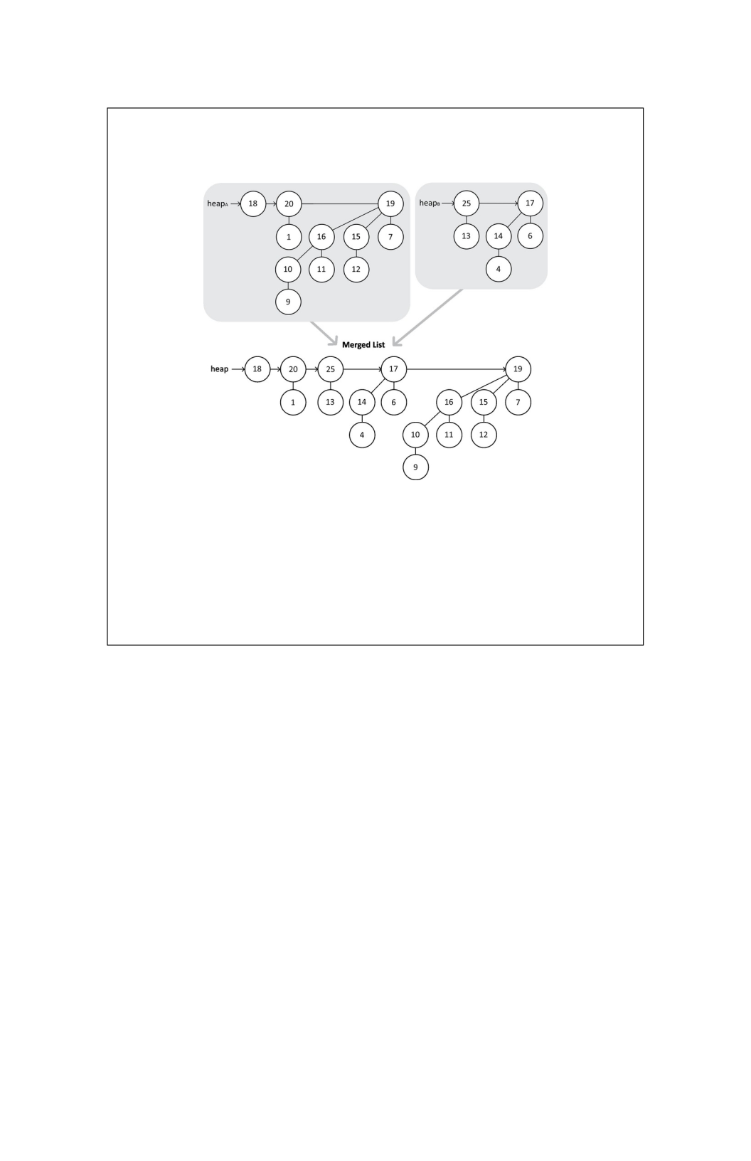
Next, the algorithm will examine two trees at a

time to determine if the trees are the same degree. Any

trees that have an equal degree will be merged.

Because the nodes are ordered by degree, we only need

to consider two nodes at a time and potentially keep track

of a carry node.

Figure 9.11

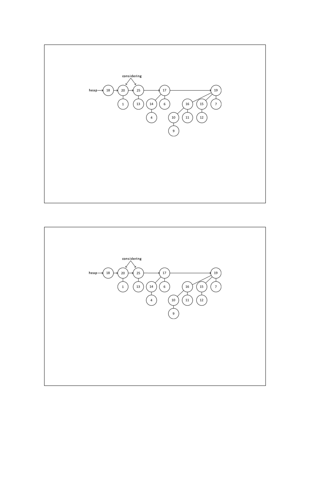
These nodes are not equal in degree. We can move on.

Now we are considering two nodes of equal degree.

These two B1 trees need to become a B2 tree.

Figure 9.12

Figure 9.13

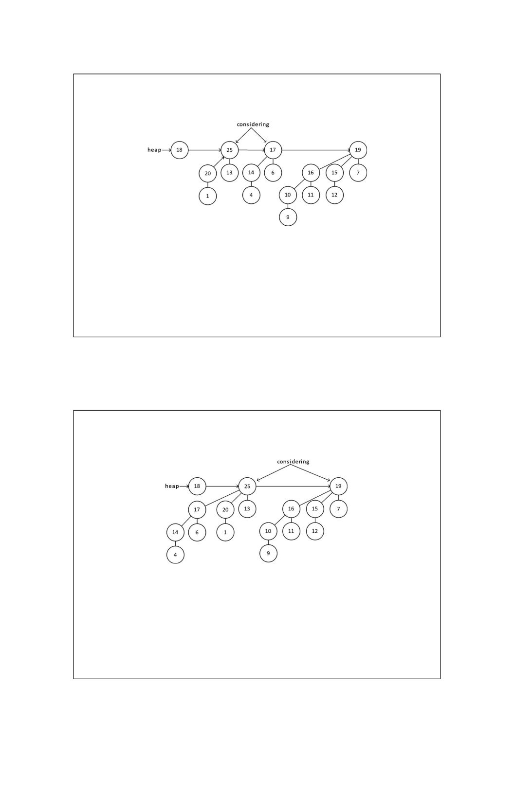
After combining the B

1

trees, we now have two B

2

trees that need to be combined. This will be done such that

the maximum item of the roots becomes the new root.

Again, the “carry” from addition means that we now have

Figure 9.14

Figure 9.15

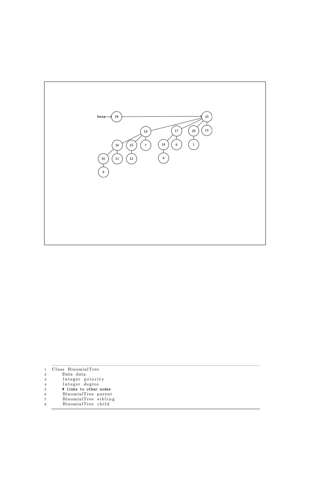
two B3 trees to merge. This step creates a B4 tree with 24 =

16 nodes. The final merged heap is below, with one B

0

node and one B

4

node:

Implementing

Binomial

Trees

To implement Binomial trees, we will need to create a node

class with appropriate links. Again, we will use references,

also known as pointers, for our links. A node—and by

extension, a tree—can be represented with the

BinomialTree class below. In this class, Data would be any

entity that needed storing in the priority queue:

Figure 9.16

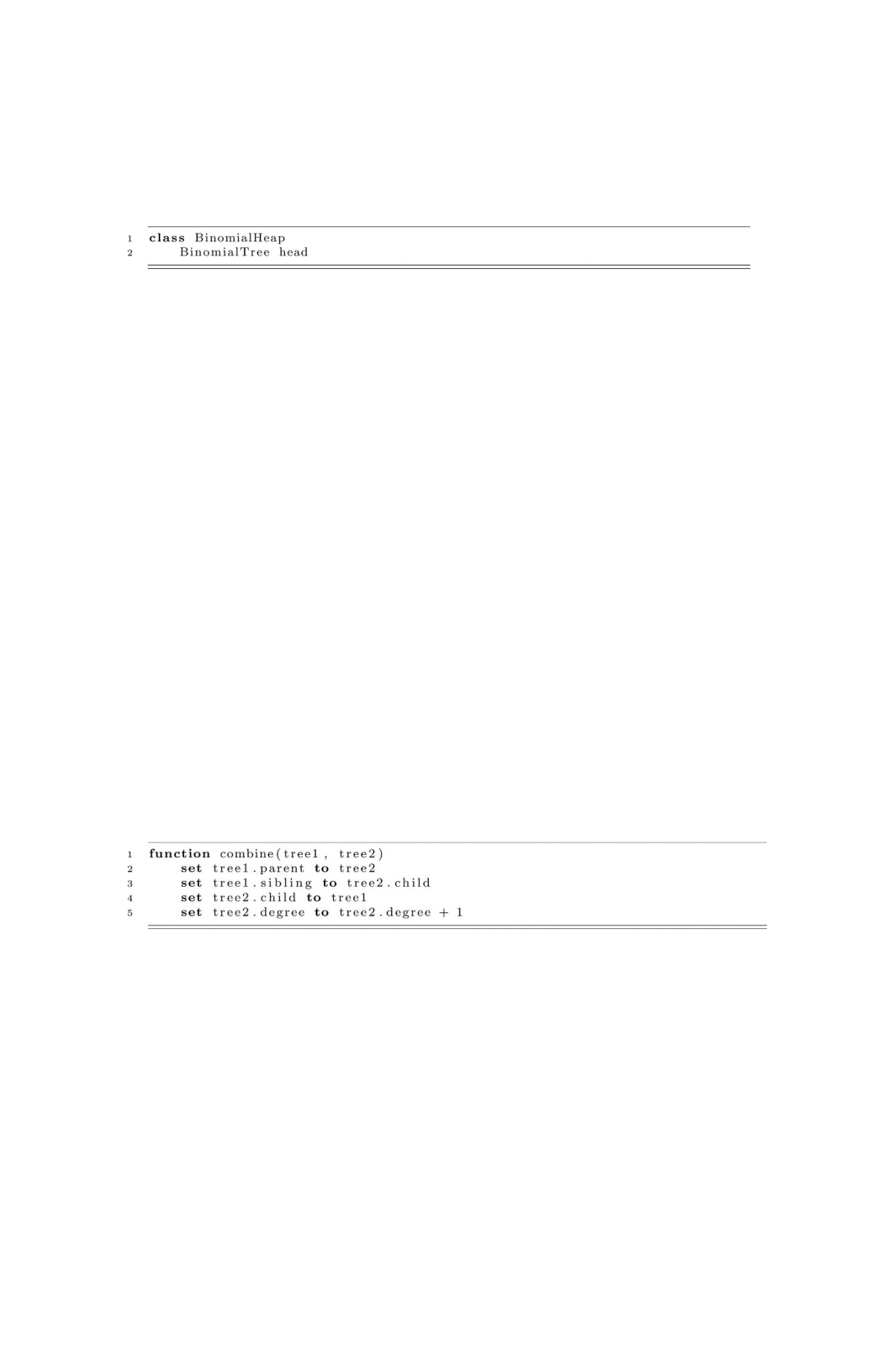
For the BinomialHeap itself, we only need a

reference to the first tree in the forest. This simple

pseudocode is presented below:

As we progress toward a complete implementation,

we will build up the operation that we need, working

toward the union operation. Once union is implemented,

adding or removing items from the heap can be

implemented through the clever usage of union. For now,

let’s implement the combine and merge functions.

Combining

Two

Binomial

Trees

The combine function is given below. This simple function

combines two Bk−1 trees to create a new Bk tree. This

function will make the first tree a child of the second tree.

We will assume that tree1.priority is always less than or

equal to tree2.priority.

The figure below shows how two B

2

trees would be

combined to form a B

3

tree. This figure also identifies the

parent, sibling, and child links for each node. Links that

do not connect to any other node have the value null. This

figure can help you understand the combine function. We

need to maintain these links in a specific way to make the

other operations function correctly. Notice that the children

of the root are all linked together by sibling links, like a

linked list’s next reference.

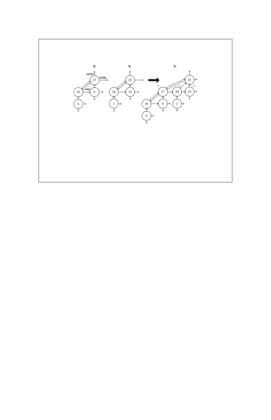
Another interesting feature of binomial trees is that

each tree of degree k contains subtrees of all the degrees

below it. These are the children linked from the first child

of the new tree. For example, the B3 tree contains a B0, B1,

and B2 subtree in descending order. You can observe these

in the figure above. This fact will come in handy when we

implement the extract function for binomial heaps.

Merging

Heaps

Now that we can combine two trees to form a higher-

degree tree, we should implement the mergeHeaps

function. This will take both heaps and their forests of

binomial trees and merge them. You can think of these

“forests” as linked lists of binomial trees. Once these

forests are merged, trees of equal degree will be

adjacent in the list. This sets the stage for our “binary

addition” algorithm that will calculate the union of both

heaps. The code for mergeHeaps is below:

Figure 9.17

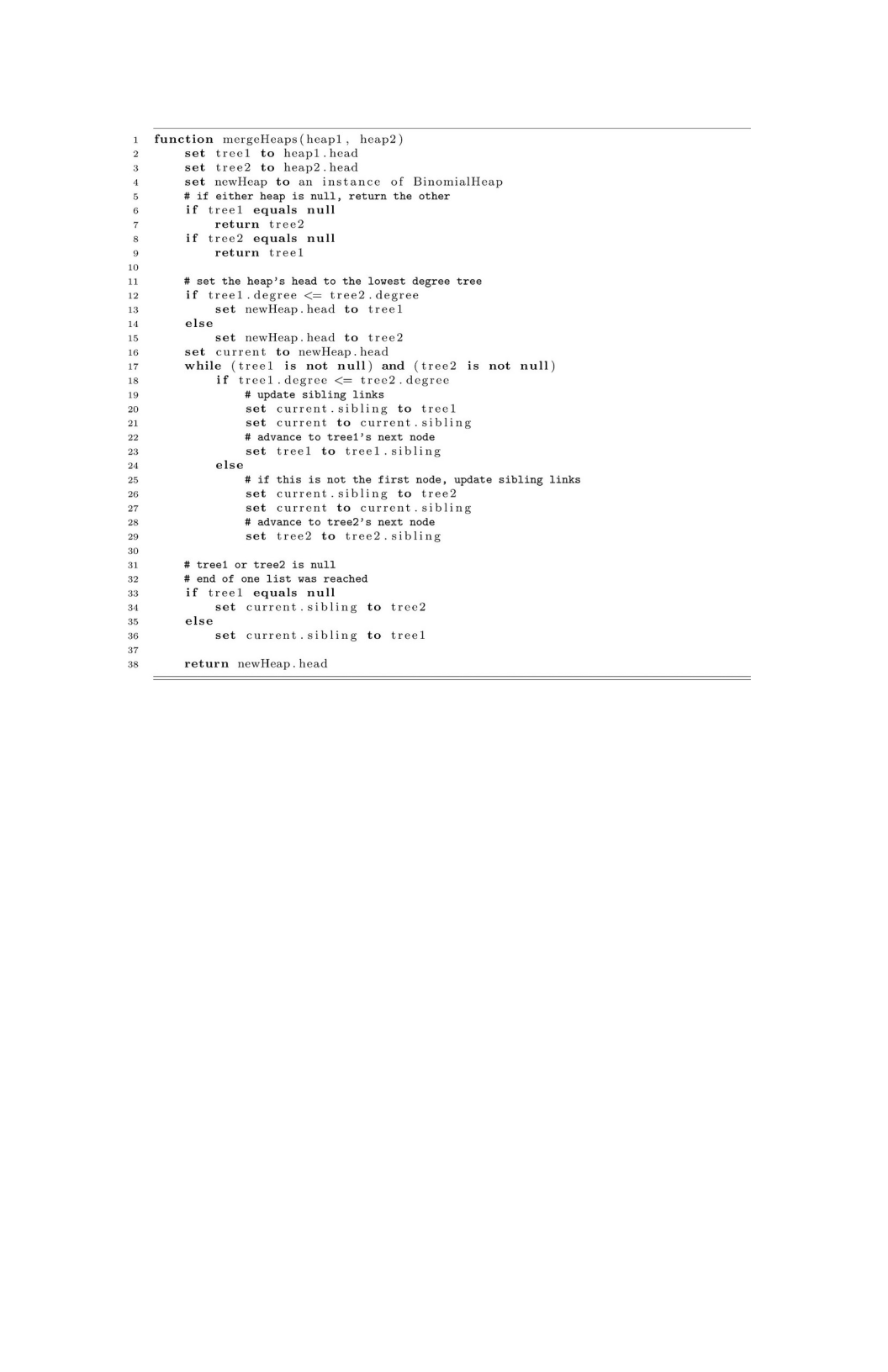
This may look a little difficult to follow, but the

concept is simple. Starting with links to the lists of binomial

trees, we first check to see if any of these are null. If so, we

just return the other one. Afterward, we check which of the

nonnull trees has the lowest degree and set our newHeap’s

head to this tree. The while-loop then appends the tree

with the next smallest degree to the growing list. The loop

continues until one of the two lists of trees reaches its end.

After that, the remaining trees are linked to the list by the

current reference, and the head of our merged list is

returned. Notice that the sibling references serve the same

role as the next pointers of a linked list.

The

Binomial

Heap

Union

Operation

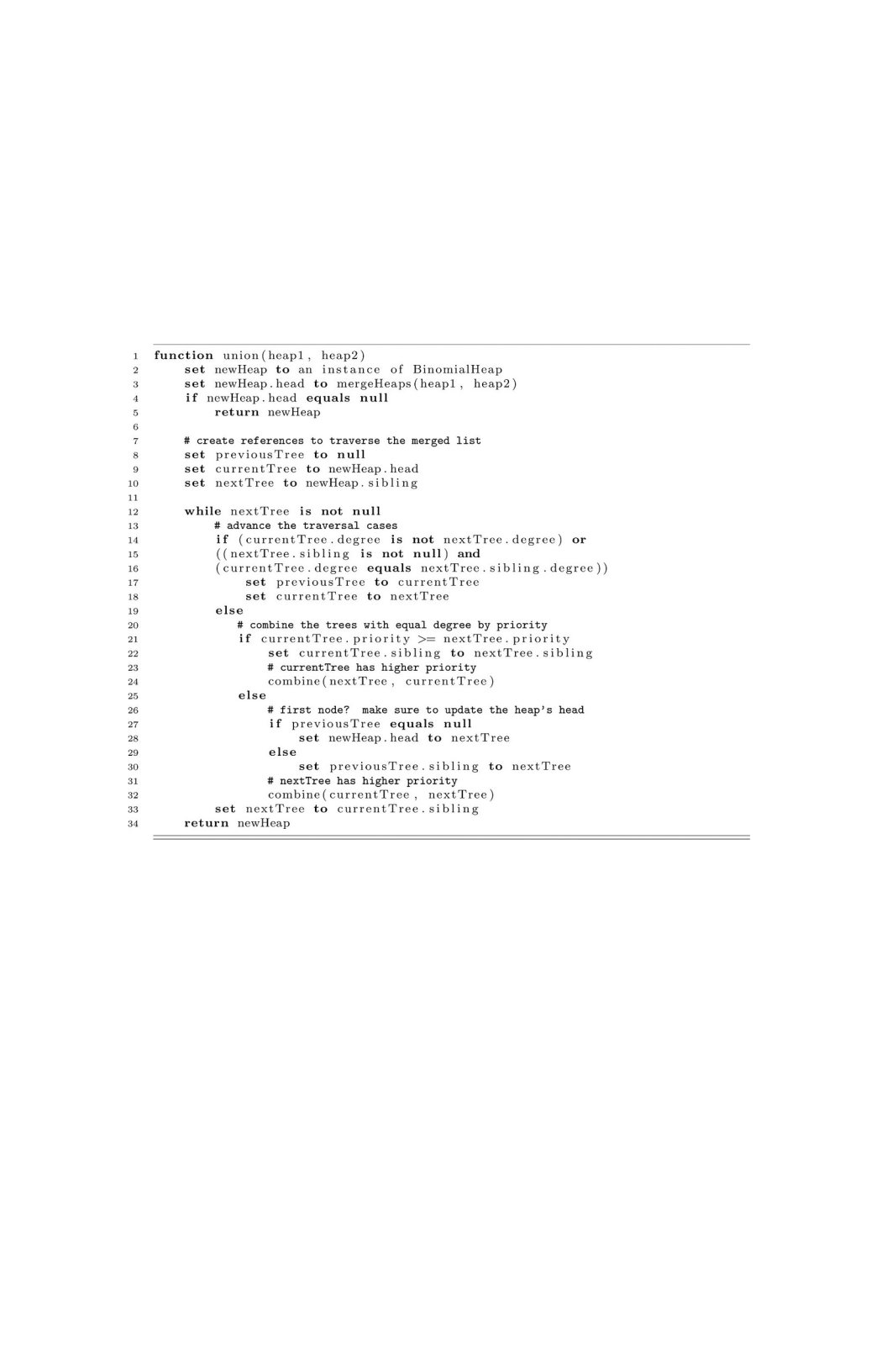
Now we will tackle the union function. This function

performs the final step of combining two binomial heaps by

traversing the merged list and combining any pairs of trees

that have equal degrees. The algorithm is given below:

The union function begins by setting up a new, empty

heap and then merging the two input heaps. Once the

merged list of trees is generated, the algorithm traverses the

list using three references (previousTree, currentTree, and

nextTree). The code will advance the traversal forward if

currentTree and nextTree have different degree values.

Another case that moves the traversal forward is when

nextTree.sibling has the same degree as currentTree and

nextTree. This is because nextTree and nextTree.sibling will

need to combine to occupy the k + 1 degree level. When a

call to combine

is needed, the algorithm checks which tree has the highest

priority, and that tree’s root becomes the root of the k +

1 tree.

Time

Complexity

of

Union

The union operation is completed, but now we should analyze

its complexity. One of the main reasons for choosing a

binomial heap was its fast union operation. How fast is it

though? We will be interested in the time complexity of union.

The algorithm traverses both heaps for the merge and the

sequence combinations. This means that the complexity is

proportional to the number of trees. We need to determine

how many binomial trees are needed to represent all n

elements of the priority queue. Recall that there are many

parallels between binomial heaps and binary numbers. If we

have 3 items in our heap, we need a tree of degree 0 with 1

item and a tree of degree 1, with 2 items. To store 5 items,

we would need a degree 0 tree with 1 item, and a degree 2

tree with 4 items. Here we see that the binary representation

of n indicates which trees of any given degree are needed to

store those elements. A number can be represented in binary

using a maximum number of bits proportional to the log of

that number. So there are log n trees in a binomial heap with

n elements. This means that the time complexity of union is

bounded by O(log n). By similar reasoning, the time cost for

finding the element with the highest priority is O(log n), the

number of binomial trees in the heap.

Inserting

into

a

Binomial

Heap

With union completed, we can see the benefit of this

operation. Below is an implementation of insert using

union. The union operation takes O(log n) time, and all

other operations can be

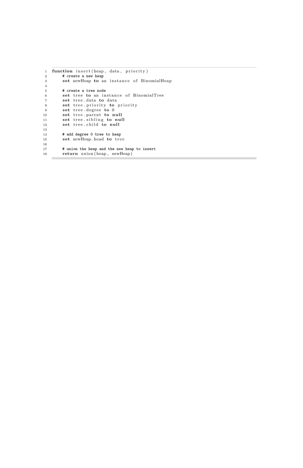
performed in O(1) time. This makes the time complexity

for insert O(log n).

Extracting

the

Max-Priority

Element

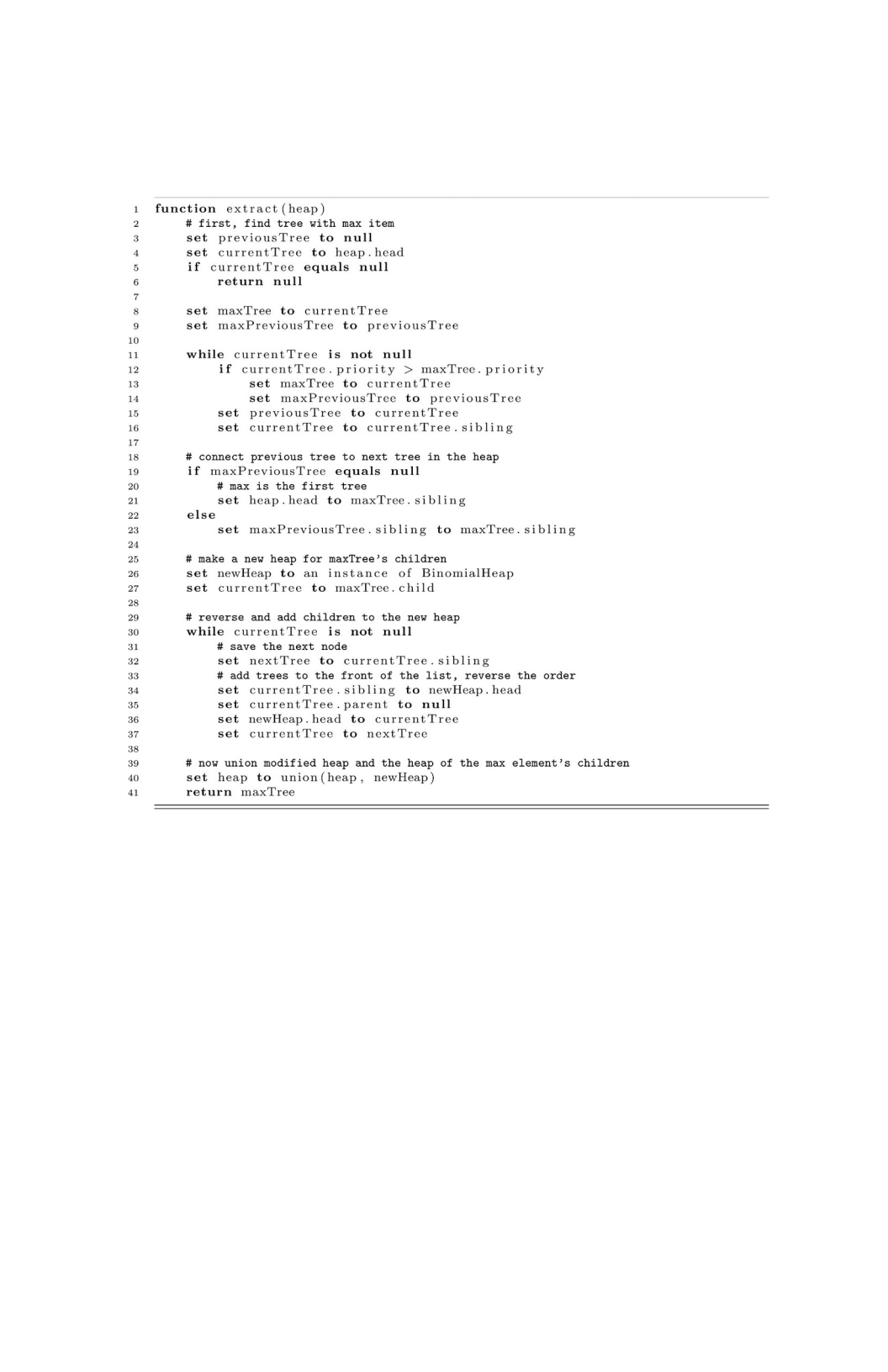
The priority queue would not be complete without a

function to extract the maximum element from the heap.

The extract function takes a bit more work, but

ultimately extract executes in O(log n) time. The

maximum priority element must be the root of one of

the heap’s trees. This function will find the maximum

priority element and remove its entire tree from the heap’s

tree list. Next, the children of the max-element are

inserted into another heap. With the two valid heaps, we

can now call union to create the binomial heap that results

from removing the highest priority element. This element

can be returned, and the binomial heap will have been

updated to reflect its new state. We note that in this

implementation, there is a side effect of extract. This

function returns the maximum priority element and

removes it from the input heap as a side effect that

modifies the input. Another approach would be to

implement an accessMax function to find the maximum

priority element and return it without updating the heap.

This means that extracting the element would require a

call to accessMax to save the element, and then extract

would be called.

We could also consider extracting part of the BinomialHeap

class and avoid passing any heap as input.

Increase-Priority

and

Delete

Operations

We will continue our theme of building new operations by

combining old ones. Here we will present the delete

operation. This operation will make use of extract and

increasePriority, which we will develop next. Creating the

increasePriority function will rely on the parent points that

we have been maintaining. When the priority of an

element is increased, it may need to work its way up the

tree structure toward the root. The following code gives an

implementation of increasePriority. We assume for

simplicity that

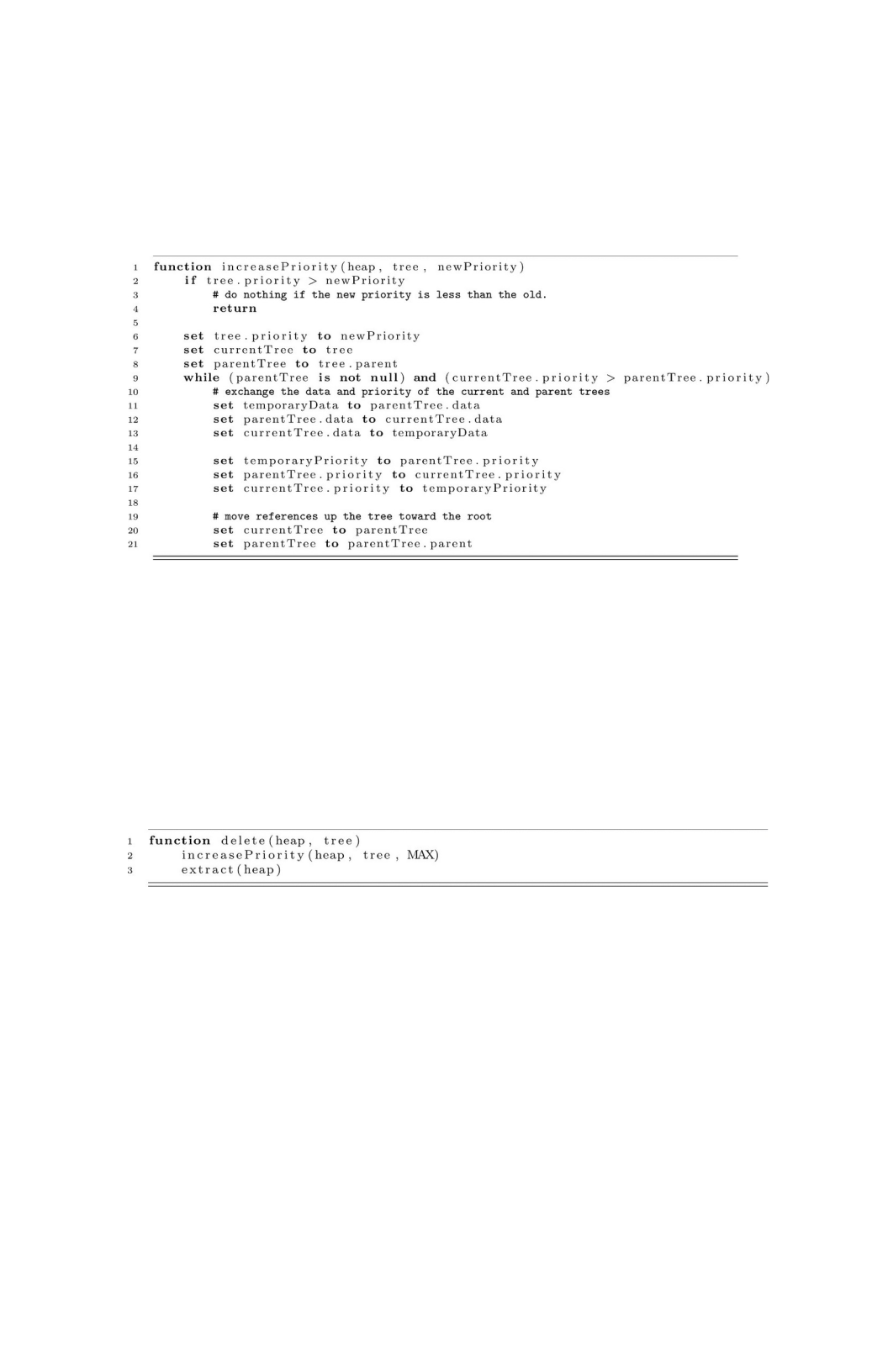
we already have a link to the element whose priority we

want to increase. The element with the highest priority

moves up the tree just like in the binary heap’s siftUp

operation.

Now we can implement delete very easily using the

MAX special value. We increase the element’s priority to

the maximum possible value and then call extract. An

implementation of delete is

provided below. Again, we

assume that a link to the element we wish

to delete is

provided.

The time complexity of delete is derived from the

complexity of increasePriority and extract. Each of these

requires O(log n) time.

Recursion

and

Dynamic

Programming

Recursive algorithms solve problems by breaking them

into smaller subproblems and then combining them.

Solving the subproblems is done by applying the same

recursive algorithm to the smaller subproblems by

breaking the subproblems into sub-subproblems. This

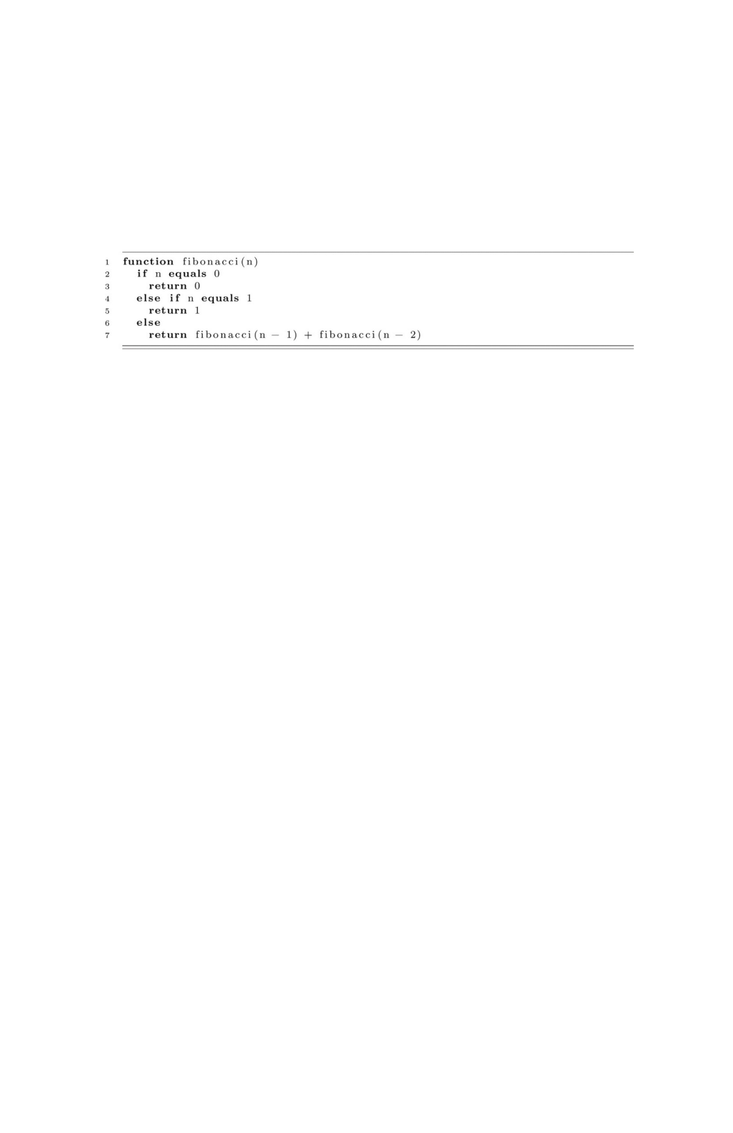
continues until the base case is reached. Below is a

recursive algorithm from chapter 2 for calculating the

Fibonacci numbers:

To solve the problem for fibonacci(n), we need

to solve it for fibonacci(n − 1) and fibonacci(n − 2). We

see that there are subproblems with the same structure as

the original problem.

The Fibonacci numbers algorithm is not an

optimization problem, but it can give us some insight to

help understand how dynamic programming can help us.

Let’s look at a specific instance of this problem. The

recursive formula for Fibonacci numbers is given below:

Now let’s explore calculating the eighth Fibonacci number:

There are two key thoughts we can learn from this

expansion for calculating F

8

. The first thought is that things

are getting out of hand and fast! Every term expands into

two terms. This leads to eight rounds of doubling. Our

complexity looks like O(2n), which should be scary. Already

at n = 20, 2

20

is in the millions, and it only gets worse from

there. The second thought that comes to mind in observing

this explanation is that many of these terms are repeated.

Let’s look at the last line again.

F0 = 0

F1 = 1

Fn = Fn−1 + Fn−2.

F8=F8−1 + F8−2

=F7 + F6

=(F7−1 + F7−2) + (F6−1 + F6−2)

=(F6 + F5) + (F5 + F4)

=((F6−1 + F6−2) + (F5−1 + F5−2)) + ((F5−1 +

F5−2) + (F4−1 + F4−2))

=((F5 + F4) + (F4 + F3)) + ((F4 + F3) + (F3 + F2))

…and so on.

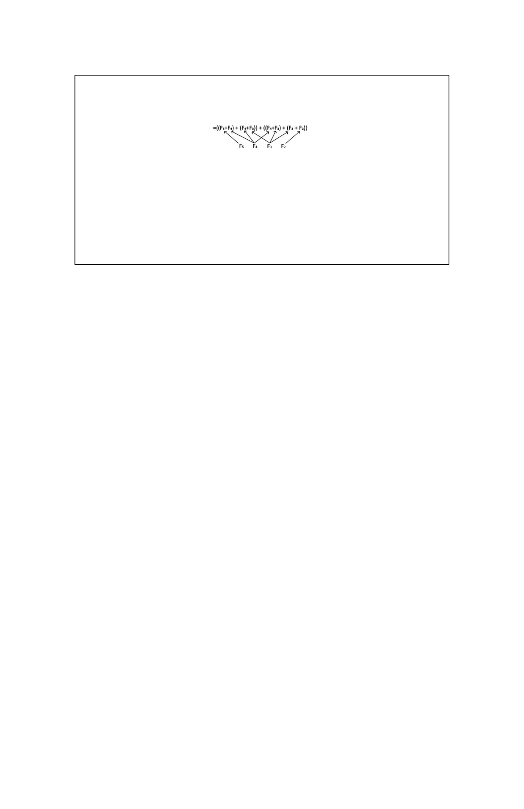
Already, we see that F

4

and F

3

are used three times

each, and they would also be used in the expansion of F

5

and F

4

. If we could calculate each of these just once and

reuse the value, a lot of computation could be saved. This

is the big idea of dynamic programming.

In dynamic programming, a record-keeping system

is employed to avoid recalculating subproblems that have

already been solved. This means that for dynamic

programming to be helpful, subproblems must share sub-

subproblems. In these cases, the subproblems are not

independent of one another. There are some repeated

identical structures shared by multiple subproblems. Not

all recursive algorithms satisfy this property. For example,

sorting one-half of an array with Merge Sort does not

help you sort the other half. With Merge Sort, each part is

independent of the other. In the case of Fibonacci, F

7

and

F

6

both share a need to calculate F

1

through F

5

. Storing

these values for reuse will greatly improve our calculation

time.

Figure 10.1

Requirements for Applying

Dynamic Programming

There are two main requirements for applying dynamic

programming. First, a problem must exhibit the property

known as optimal substructure. This means that an

optimal solution to the problem is constructed from

optimal solutions to the subproblems. We will see an

example of this soon. The second property is called

overlapping subproblems. This means that subproblems

are shared. We saw this in our Fibonacci example.

Optimal Matrix Chain Multiplication

A classic application of dynamic programming concerns

the optimal multiplication order for matrices. Consider the

sequence of matrices {M1, M2, M3, M4}. There are several

ways to multiply these together. These ways correspond

to the number of distinct ways to parenthesize the matrix

multiplication order. For the mathematically curious, the

Catalan numbers give the total number of possible ways.

For example, one way to group these would be (M

1

M2) (M3

M4). Another way could be M1 ((M2 M3) M4). Any grouping

leads to the same final result, but the number of multiply

operations of the overall calculation could differ greatly

with different groupings. To understand this idea, let’s

review matrix multiplication.

Matrix

Multiplication

Review

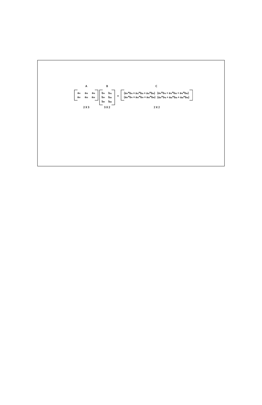
Matrix multiplication is an operation that multiplies and adds the

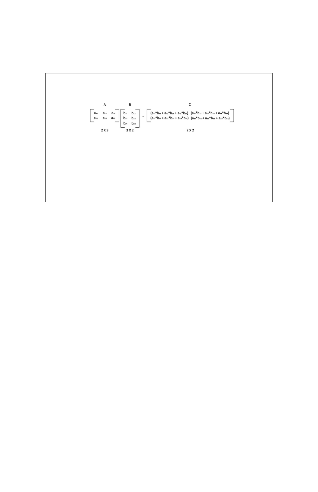
rows of one matrix with the columns of another matrix.

Below is an example:

Here we have the matrix A and the matrix B. A is a

2-by-3 matrix (2 rows and 3 columns), and B is a 3-by-2

matrix (3 rows

and 2 columns). The multiplication of AB is

compatible, which means

the number of columns of A is

equal to the number of rows in the second matrix, B. When

two compatible matrices are multiplied, their result has a

structure where the number of rows equals the number of

rows in the first matrix and the number of columns equals

the number of columns in the second matrix. The process

is the same for compatible matrices of any size.

Implementing

Matrix

Multiplication

Now let’s consider an algorithm for matrix multiplication.

To simplify things, let’s assume we have a Matrix class or

data structure that has a two-dimensional (2D) array.

Another way to think of a 2D array is as an array of

arrays. We could also think of this as a table with rows

and columns. The structure below gives a general example

of a Matrix class. Within this class, we also have

Figure 10.2

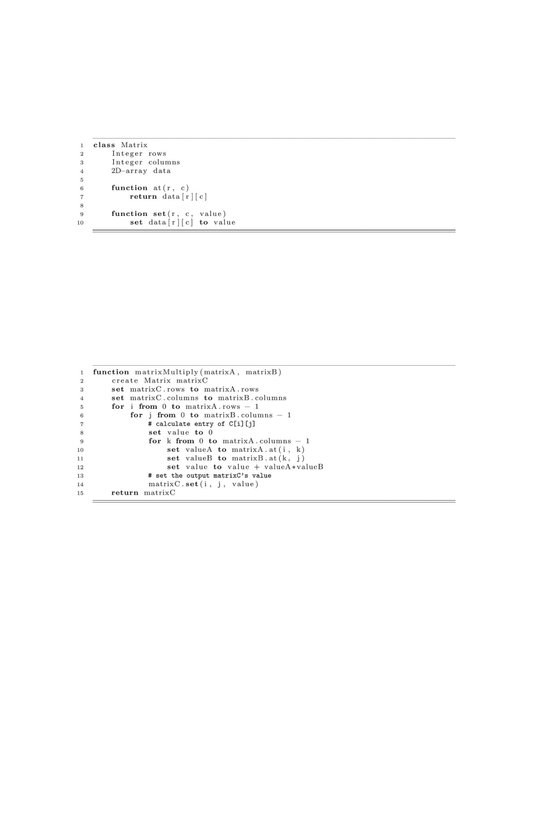
two convenience functions to access and set the values

of the matrix based on the row and column of the 2D

array.

With this structure for a Matrix class, we can

implement a matrix multiplication procedure. Below we

show the process of performing matrix multiplication on

two compatible matrices:

This function implements the matrix multiplication

procedure described above. On line 12, the new value of

the (i, j) entry in the result matrix is calculated. We see

that this involves a multiply operation and an addition

operation. On a typical processor, the multiply operation is

slower than addition. As we think about the complexity of

matrix multiplication, we will mainly consider the number

of multiplications. This is because as the matrices get

large, the cost associated with multiplication will dominate

the cost of addition. For this reason, we only consider the

number of multiplications.

So

how

many

multiplications

are

needed

for

matrix

multiplication? The pattern above has a triple-nested loop.

This gives us a clue to the number of times the inner

code will run. As a result, we can expect the number of

multiplications to be equal to the number of times the

inner code will run. Let’s assume that matrix A has ra rows

and ca columns, and that matrix B, in a similar way, has rb

rows and cb columns. For A and B to be compatible

matrices, the value of ca would have to be equal to rb. We

know that the inner loop with index k runs a total of ca

times. This entire loop is executed once for every cb of B’s

columns (cb * ca). Finally, these two inner loops for j and k

would all run for every row in A, leading to multiplications

proportional to ra * ca * cb. This illustrates that as the size

of the matrices gets larger, the number of multiplications

grows quickly.

Why Order Matters

Now that we have seen how to multiply matrices together

and understand the computational cost, let’s consider just

why choosing to multiply in a specific order is important.

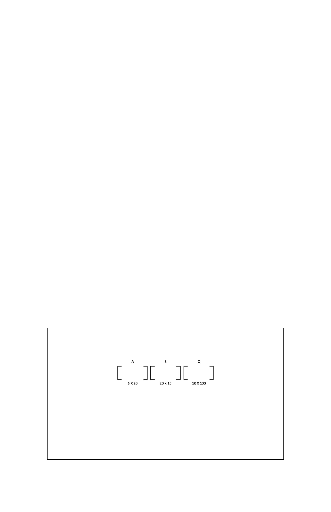
Suppose that we need to multiply three matrices—A, B,

and C—shown in the image below:

Figure 10.3

Multiplying them together could proceed with the

grouping (AB)C, where A and B are multiplied together

first, and then that result is multiplied by C. Alternatively, we

could group them as A(BC) and first multiply B by C, followed

by A multiplied by the result. Which would be better, or

would it even matter?

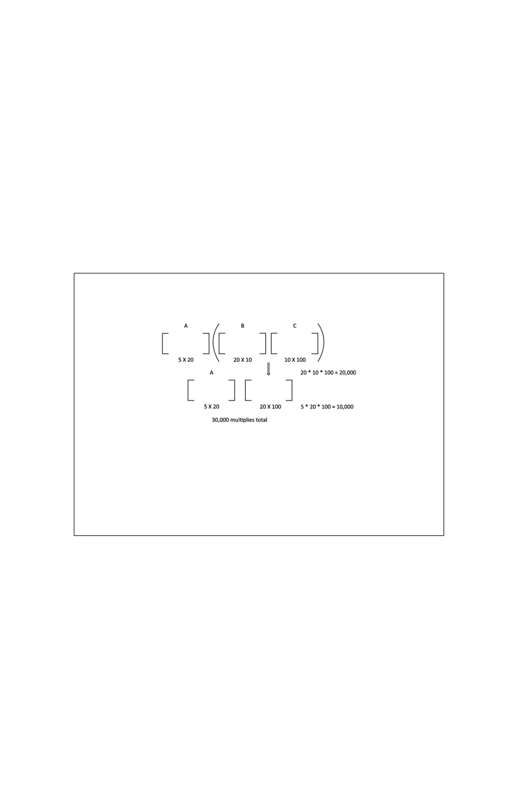
Let’s figure this out by first considering the A(BC)

grouping. The figure below illustrates this example. With

this grouping, calculating the BC multiplication yields

20,000 multiply operations. Multiplying A by this result

gives another 10,000 for a total of 30,000 multiply

operations.

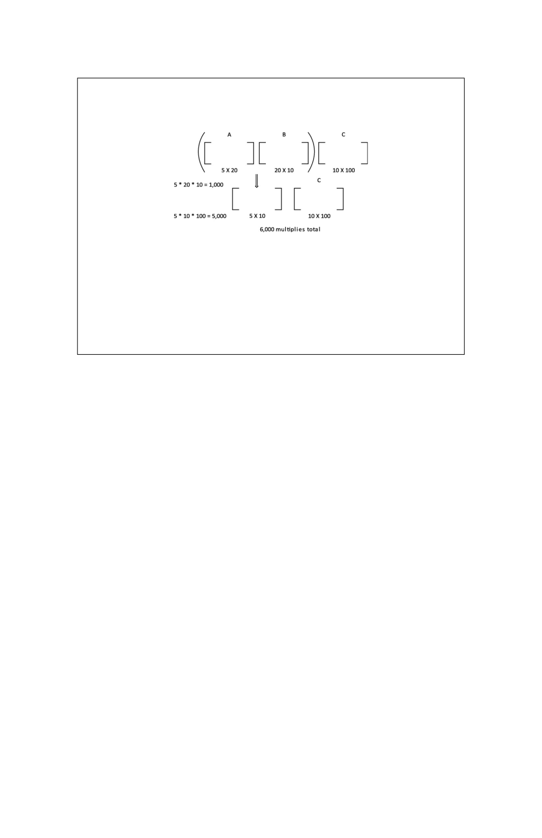
Next, let’s consider the (AB)C grouping. The following

figure

shows a rough diagram of this calculation. The AB

matrix multiplication gives a cost of 1,000 multiply

operations. Then this result multiplied by C gives another

5,000. We now have a total of 6,000 multiply operations

for the (AB)C grouping over the other. This represents a

fivefold decrease in cost!

Figure 10.4

This example illustrates that the order of

multiplication definitely matters in terms of computational

cost. Additionally, as the matrices get larger, there could

be significant cost savings when we find an optimal

grouping for the multiplication sequence.

A Recursive Algorithm

for Optimal Matrix-Chain

Multiplication

We are interested in an algorithm for finding the optimal

ordering of matrix multiplication. This corresponds to

finding a grouping with a minimal cost. Suppose we have a

chain of 5 matrices, M

0

to M

4

. We could write their

dimensions as a list of 6 values. The 6 values come from

the fact that each sequential pair of matrices must be

compatible for multiplication to be possible. The figure

below shows this chain and gives the dimensions as a list.

Figure 10.5

An algorithm that minimizes the cost must find an

optimal split for the final two matrices. Let’s call these final

two matrices A and B. For the result to be optimal, then A

and B must both have resulted from an optimal subgrouping.

The possible splits would be

We need to evaluate these options by assessing

the cost of creating the A and B matrices (optimal

subproblems) as well as the cost of the final multiply, with

matrix A being multiplied by B. A recursive algorithm

would find the minimal cost by checking the minimum cost

among all splits. In the process of finding the cost of all

these four options for splits, we would need to calculate

the optimal splits for other sequences to find their optimal

groupings. This demonstrates the feature of optimal

substructure, the idea that an optimal solution could be

Figure 10.6

(M0) (M1 M2 M3 M4) = AB with a split after

position 0 (M0 M1) (M2 M3 M4) = AB with a split

after position 1 (M0 M1 M2) (M3 M4) = AB with a

split after position 2 (M0 M1 M2 M3) (M4) = AB

with a split after position 3.

built from optimal subproblems.

For the first grouping, we have A = M0 and B = (M1

M2 M3 M

4

). To calculate the cost of this split, it is

assumed that A and B have been constructed optimally.

This means that a recursive algorithm considering this split

must then make a recursive call to

find the minimal

grouping for (M1 M2 M3 M4) for the B matrix. This in

turn

would trigger another search for the optimal split among

(M

1

) (M2 M3 M4) (M1 M2) (M3 M4) and (M1 M2 M3) (M4). We

can also see

that this would trigger further calls to optimize each

sequence of 3 matrices and so on. You may be able to

imagine that this recursive process has a high branch

factor leading to an exponential runtime complexity in the

number of matrices. With n matrices, the runtime

complexity would be even worse than O(2n), exponential time. It

would follow an algorithm for calculating the Catalan

numbers at O(3n).

A general outline of the recursive algorithm would be

as follows. We will consider an algorithm to calculate the

minimal cost of multiplying a sequence of matrices starting at

some matrix identified by the start index and including the

ending matrix using an end index. The base case of the

algorithm is when start and end are equal. The cost of

multiplication of only one matrix is 0 as there is no

operation to perform. The recursive case calculates the cost

of splitting the sequence at some split position. There will be

n − 1 split positions to test when considering n matrices

where n = end − start

+ 1, and the recursive algorithm will need to find the

minimum of the options for the best split position.

To complete the recursive algorithm, we will

introduce a function to calculate the cost of the final

multiplication. This could be a simple multiplication of the

correct dimensions, but we will introduce and explain this

function to make the meaning clear and to simplify some

of the code (which would otherwise include a lot of

awkward indexing). The figure below illustrates what is

meant by the final multiplication:

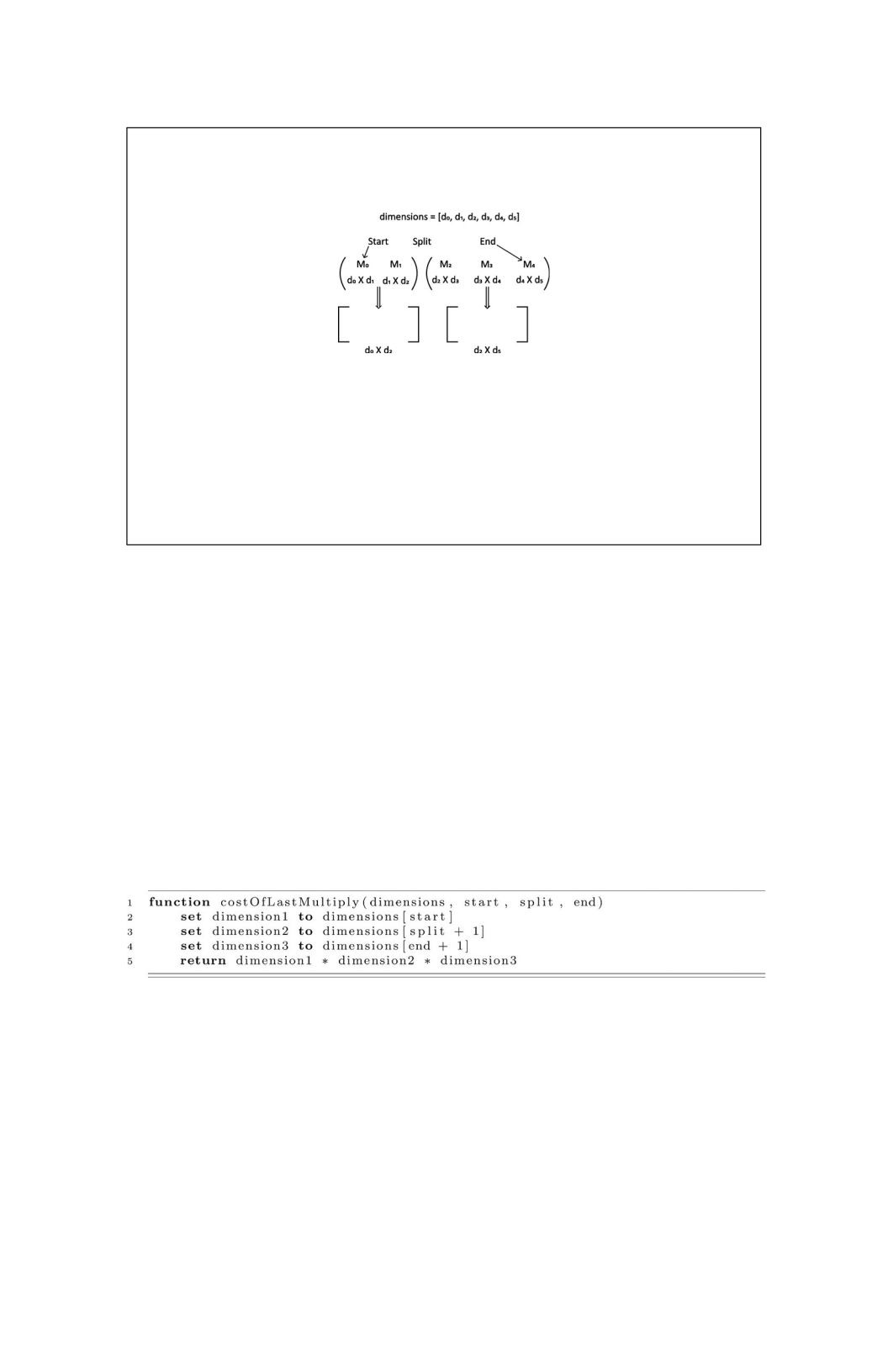
Suppose we are calculating the number of

multiplications for a split at index 1 (or just after M1). The

algorithm would have given the optimal cost for constructing

the left matrix and the right matrix, but we would still need to

calculate the cost of multiplying those together. The left

matrix would have dimensions of d0 by d2 and the right

matrix would have dimensions of d2 by d5. Using the

dimensions list and indexes for start, split, and end, we can

calculate this cost. The function below performs this operation

in a way that might make the meaning a little clearer. Notice

that for matrix i, the dimensions of that matrix are di by di+1.

With this helper function, we can now write the

recursive algorithm.

Figure 10.7

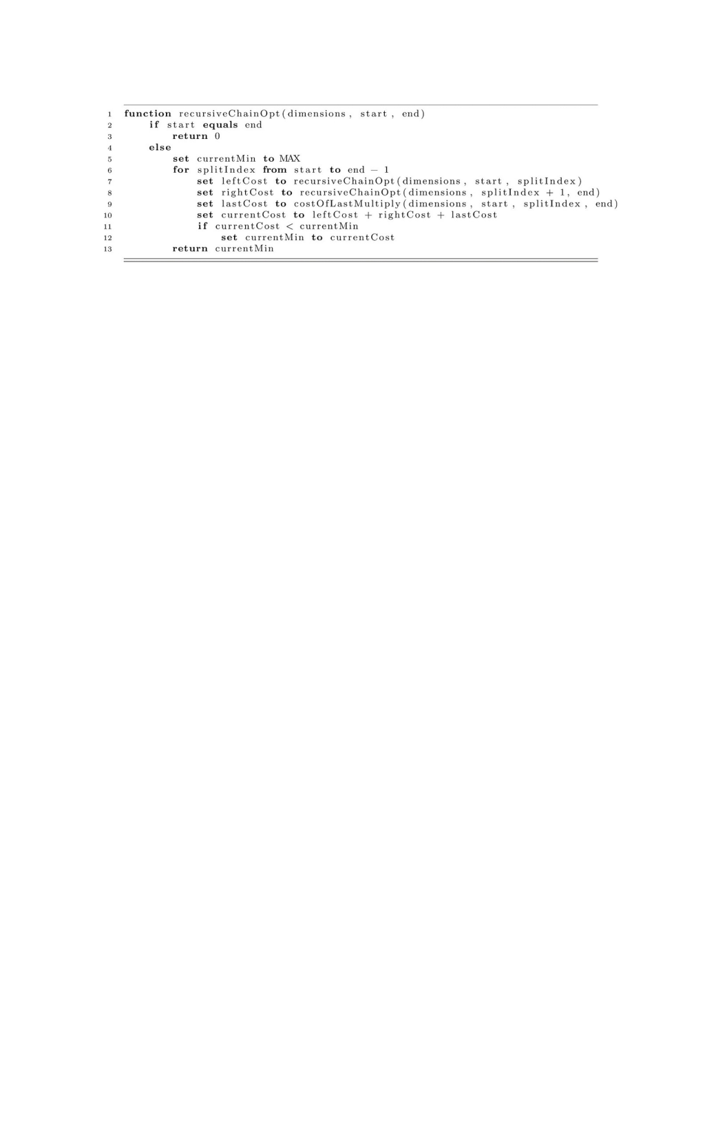
This algorithm only calculates an optimal cost, but

it could be modified to record the split indexes of the

optimal splits so that another process could use that

information. The optimal cost of multiplying all matrices in

the optimal grouping could be calculated with a call to

recursiveChainOpt(dimensions, 0, 4). This algorithm, while

correct, suffers from exponential time complexity. This is

the type of situation where dynamic programming can

help.

A

Dynamic

Programming

Solution

Let’s think back to our precious example for a moment.

Think specifically about the first two groupings we wanted

to consider. These are (M0) (M1 M2 M3 M4) and (M0 M1) (M2

M3 M4). For the first grouping, we need to optimize the

grouping of (M1 M2 M3 M4) as a subproblem. This would

involve also considering the optimal

grouping of (M2 M3 M4).

Optimally grouping (M2 M3 M4) is a problem

that must be

solved in the process of calculating the cost of (M

0

M1) (M2

M3 M4), which is the second subproblem in the original

grouping. From this, we see that there are overlapping

subproblems. Considering this problem meets the criteria

of optimal substructure and overlapping subproblems, we

can be confident that dynamic programming will give us an

advantage.

The logic behind the dynamic programming

approach is to calculate the optimal groupings for

subproblems first, working

our way through larger and larger subsequences and

saving their optimal cost. Eventually, the algorithm

minimizes the cost of the full sequence of matrix

multiplies. In this calculation, the algorithm queries the

optimal costs of the smaller sequences from a table. This

algorithm uses two tables. The first table, modeled using a

2D array, stores the calculated optimal cost of multiplying

matrices i through

j. This table will be called costs. The second table holds the

choice of split index associated with the optimal cost. This

table will be called splits. While the algorithm calculates

costs, the splits are the important data that can be used to

perform the actual multiplication in the right order.

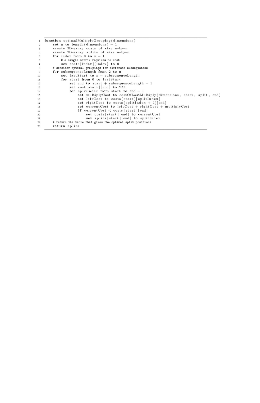
The algorithm is given below. It begins by assigning

the optimal values for a single matrix. A single matrix has

no multiplies, so when calculating a matrix chain

multiplication with a sequence of 1, the cost is 0. Next, the

algorithm sets a sequence length starting at 2. From here,

start and end indexes are set and updated such that the

optimal cost of all length 2 sequences in the chain are

calculated and stored in the costs table. Next, the

sequence length is increased to 3, and all optimal

sequences of length 3 are calculated by trying the different

options for the splitIndex. The splitIndex is updated in the

splits table each time an improvement in cost is found. We

should note that we again make use of the MAX value,

which acts like infinity as we minimize the cost for a split.

The process continues for larger and larger sequence

lengths until it finds the cost of the longest sequence, the

one including all the matrices.

Complexity of the Dynamic

Programming

Algorithm

Now we have seen two algorithms for solving the optimal

matrix chain multiplication problem. The recursive

formulation proved to be exponential time (O(2n)) with

each recursive call potentially branching n

− 1

times. The

dynamic programming algorithm should improve upon this

cost; otherwise, it would not be very useful. One way to

reason about the complexity is to think about how the

tables get filled in. Ultimately, we are filling in about one-

half of a 2D array or table. This amounts to filling in the

upper triangular portion of a matrix in mathematical

terms. Our table is n by n, and we are filling in n(n+1)/2

values (a little over half of the n-by- n matrix). So you may

think the time complexity should be O(n

2

). This is not the

full story though. For every start-end pair, we must try all

the split indexes. This could be as bad as n

− 1.

So all

these pairs need to evaluate up to n

− 1

options for a split.

We can reason that this requirement would lead to some

multiple of n

2

*n or n

3

operations. This provides a good

explanation of the time complexity, which is O(n

3

). This

may seem expensive, but O(n

3

) is profoundly better than

O(3n). Moreover, consider the difference between the

number matrices and the number multiplications needed

for the chain multiplication. For our small example of 3

matrices (our n in this case), we saw the number of

multiply operations drop by 24,000 when using the optimal

grouping, and our n was only 3. This could result in a

significant improvement in the overall computation time,

making the optimization well worth the cost.

Longest

Common

Subsequence

Another classic application of dynamic programming

involves detecting a shared substructure between two

strings. For example, the two strings “pride” and “ripe”

share the substring “rie.” For these two strings, “rie” is the

longest common subsequence or LCS. There are other

subsequences, such as “pe,” but “rie” is the longest or

optimal subsequence. These subsequence strings do not

need to be connected. They can have nonmatched

characters in between. It might seem like a fair question to

ask, “Why is this useful?” Finding an LCS may seem like a

simple game or a discrete mathematics problem without

much significance, but it has been applied in the area of

computational biology to perform alignments of genetic

code and protein sequences. A slight modification of the

LCS algorithm we will learn here was developed by

Needleman and Wunsch in 1970. That algorithm inspired

many similar algorithms for the dynamic alignment of

biological sequences, and they are still empowering

scientific discoveries today in genetics and biomedical

research. Exciting breakthroughs can happen when an old

algorithm is creatively applied in new areas.

Defining the LCS and Motivating

Dynamic

Programming

A common subsequence is any shared subsequence of two

strings. A subsequence of a string would be any ordered

subset of the original sequence. An LCS just requires that

this be the longest such subsequence belonging to both

strings. We say “an” LCS and not “the” LCS because there

could be multiple common subsequences with the same

optimal length.

Let’s add some terms to better understand the

problem. Suppose we have two strings A and B with

lengths m and n, respectively. We can think of A as a

sequence of characters A = {a

0

, a1, …, am−1} and B as a

sequence of the form B = {b0, b1, …, bn−1}. Suppose we

already know that C is an LCS of A and B. Let’s let k be the

length of C. We will let Ai or Bi mean the subsequence up to

i, or Ai = {a0, a1, …, ai}. If we think of the last element in

C, Ck−1 must be in A and B. For this to be the case, one of

the following must be true:

1. ck−1 = am−1 and ck−1 = bn−1. This means that am−1 =

bn−1 and Ck−2 is an LCS of Am−2 and Bn−2.

2.

am−1 is not equal to bn−1, and ck−1 is not equal to

am−1. This must mean that C is an LCS of Am−2 and B.

3. am−1 is not equal to bn−1, and ck−1 is not equal to bn−1.

This must mean that C is an LCS of A and Bn−2.

In other words, if the last element of C is also the

last element of A and B, then it means that the

subsequence Ck−2 is an LCS of Am−2 and Bn−2. This is

hinting at the idea of optimal substructure, where the

full LCS could be built from the Ck−2 subproblem. The

other two cases also imply subproblems where an LCS, C,

is constructed from either the case of Am−2 (A minus its

last element) and B or the case of A and Bn−2 (B minus its

last element).

Now let’s consider overlapping subproblems. We

saw that our optimal solution for an LCS of A and B could

be built from an

LCS of Am−2 and Bn−2 when the last elements of A and B

are the same. Finding an LCS of Am−2 and Bn−2 would also

be necessary for our other two cases. This means that in

evaluating which of the three cases leads to the optimal

LCS length, we would need to

evaluate the LCS of Am−2 and

Bn−2 subproblems and potentially many

other shared

problems with shorter subsequences. Now we have

some

motivation for applying dynamic programming with these two

properties satisfied.

A Recursive Algorithm for Longest

Common Subsequence

Before looking at the dynamic programming algorithm,

let’s consider the recursive algorithm. Given two

sequences as strings, we wish to optimize for the length of

the longest common subsequence. The algorithm below

provides a recursive solution to the calculation of the

optimal length of the longest common subsequence. Like

with our matrix chain example, we could add another list

to hold each element of the LCS, but we leave that as an

exercise for the reader.

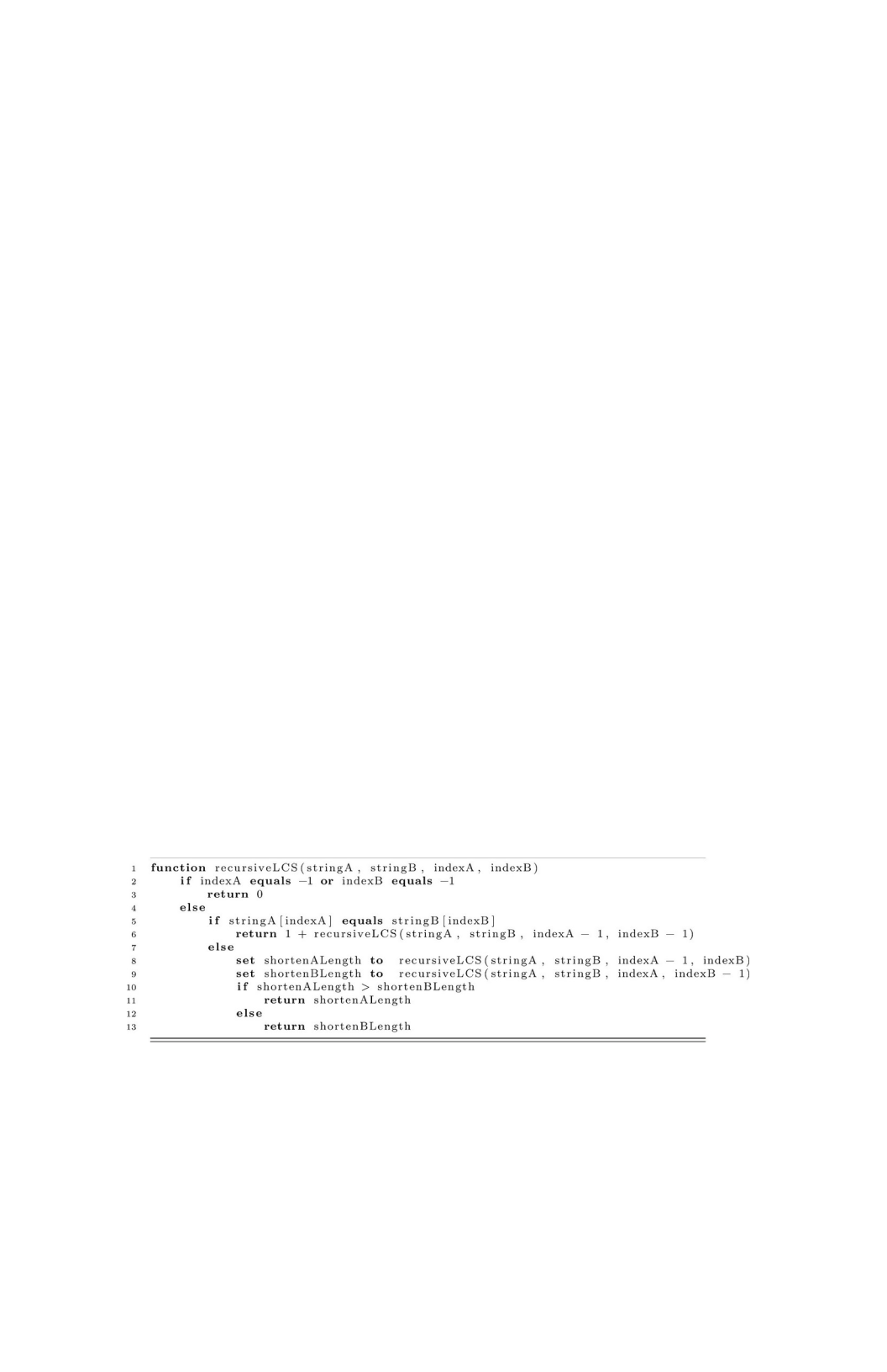
This algorithm will report the optimal length using a

function call with the last valid indexes (length − 1) of

each string provided as the initial index arguments. For

example, letting A be

“pride” and B be “ripe,” our call would be recursiveLCS(A, B,

4, 3), with 4 and 3 being the last valid indexes in A and B.

Trying to visualize the call sequence for this recursive

algorithm, we could image a tree structure that splits into

two branches each time the else block is executed on line

7. In the worst case, where there are no shared elements

and the length of an LCS is 0, this means a new branch

generates 2 more branches for every n elements

(assuming n is larger than m). This leads to a time complexity

of O(2n).

A

Dynamic

Programming

Solution

In a similar way to the matrix chain algorithm, our dynamic

programming solution for LCS makes use of a table to

record the length of the LCS for a specific pair of string

indexes. Additionally, we will use another “code” table to

record from which optimal subproblem the current optimal

solution was constructed.

The following dynamic programming solution tries

to find LCS lengths for all subsequences of the input strings

A and B. First, a table, or 2D array, is constructed with

dimensions (n+1) by (m+1). This adds an extra row and

column to accommodate the LCS of a sequence and an

empty sequence or nothing. A string and the empty string

can have no elements in common, so the algorithm

initializes the first row and column to zeros. Next, the

algorithm proceeds by attempting to find the LCS length of

all subsequences of string A and the first element of string

B. For any index pair (i, j), the algorithm calculates the

LCS length for the two subsequence strings Aj and Bi.

The core of the algorithm checks the three cases

discussed above. These are the case of a match among

elements of A and B and two other cases where the

problem could be reformulated as either shortening the A

string by one or shortening the B string by one. As the

algorithm decides which of these options is optimal, we

record a value into our “code” table that tells us which of

these options was

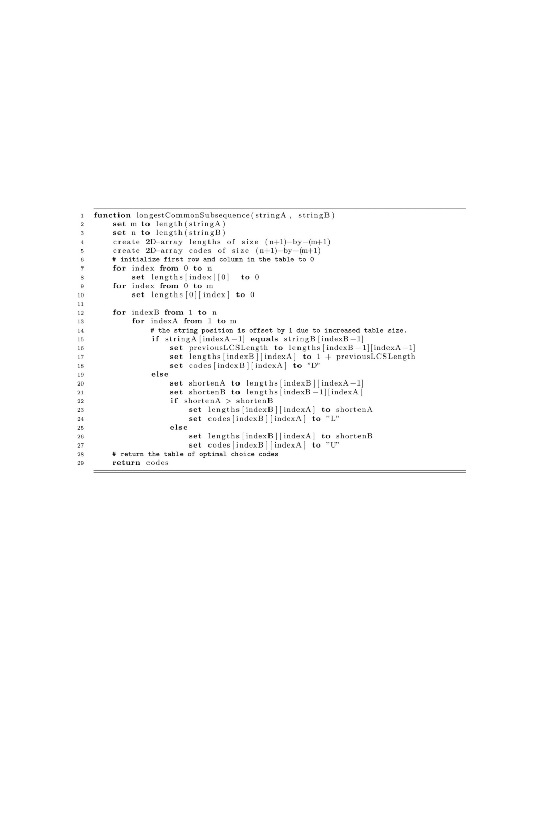
chosen. We will use the code “D,” “U,” and “L” for

“Diagonal,” “from the Upper entry,” and “from the Left

entry.” These codes will allow us to easily traverse the

table by moving “diagonal,” “up,” or “left,” always taking

an optimal path to output an LCS string. Let’s explore the

algorithm’s code and then try to understand how it works

by thinking about some intermediate states of execution.

To better understand the algorithm, we will explore

our previous example of determining the LCS of “pride”

and “ripe.” Let us imagine that the algorithm has been

running for a bit and we are now examining the point

where indexB is 2 and indexA is 4. The figure below gives a

diagram of the current states of the lengths and codes

tables at this point in the execution:

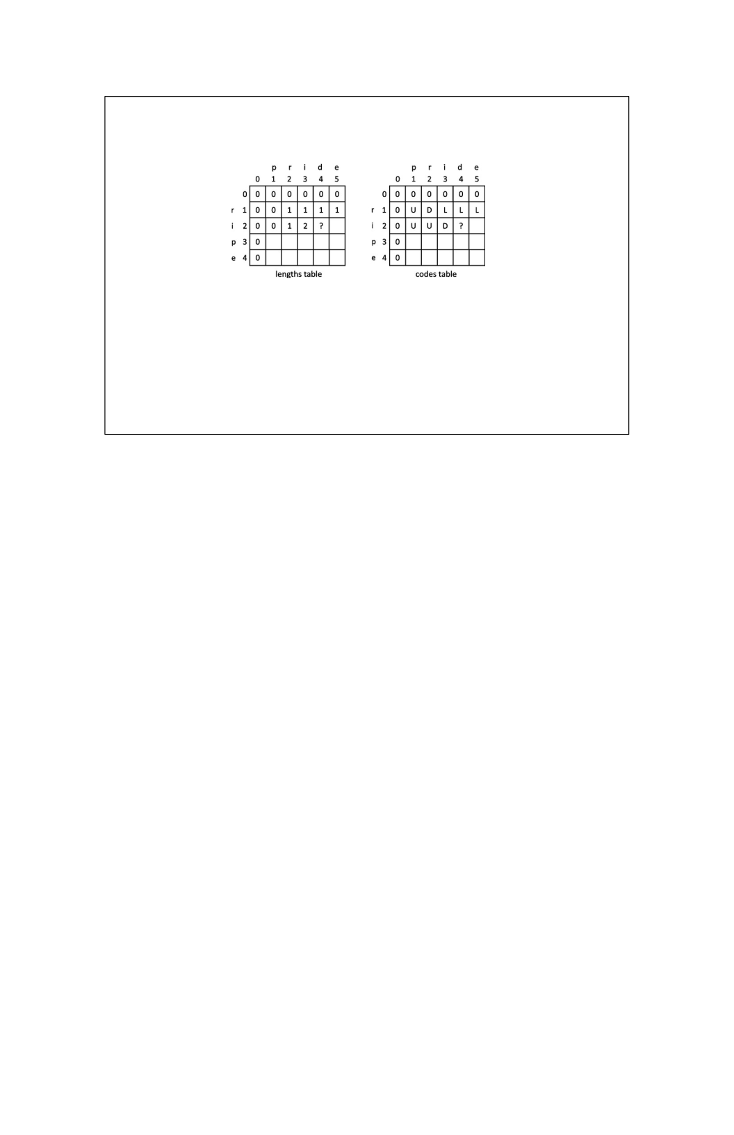
These tables can give us some intuition on how

the algorithm works. Looking at the lengths table in row 2

and column 2, we see there is a 1. This represents the LCS of

the strings “pr” and “ri.” They share a single element “r.”

Moving over to the cell found in row 2 and column 3, we see

the number 2. This represents the length of the LCS of the

strings “pri” and “ri.” Now the algorithm is considering the

cell in the row 2 column 4 position. The strings in these

positions do not match, so this is not built from the LCS along

the diagonal. The largest LCS value from the previous

subproblems is 2. This means that the LCS of “prid” and

“ri” is the same as the LCS of the shortened A string “pri”

and “ri.” Since this is the case, we would mark a 2 at this

position in the lengths table and make an “L” in this position

in the codes table. These algorithms take time to understand

fully. Don’t get discouraged if it doesn’t click right away. Try

to implement it in your favorite programming language, and

work on some examples by hand. Eventually, it will become

clear.

Requirements for Applying

Figure 10.8

Dynamic Programming

There are two main requirements for applying dynamic

programming. First, a problem must exhibit the property

known as optimal substructure. This means that an

optimal solution to the problem is constructed from

optimal solutions to the subproblems. We will see an

example of this soon. The second property is called

overlapping subproblems. This means that subproblems

are shared. We saw this in our Fibonacci example.

Optimal Matrix Chain Multiplication

A classic application of dynamic programming concerns

the optimal multiplication order for matrices. Consider the

sequence of matrices {M1, M2, M3, M4}. There are several

ways to multiply these together. These ways correspond

to the number of distinct ways to parenthesize the matrix

multiplication order. For the mathematically curious, the

Catalan numbers give the total number of possible ways.

For example, one way to group these would be (M

1

M2) (M3

M4). Another way could be M1 ((M2 M3) M4). Any grouping

leads to the same final result, but the number of multiply

operations of the overall calculation could differ greatly

with different groupings. To understand this idea, let’s

review matrix multiplication.

Matrix

Multiplication

Review

Matrix multiplication is an operation that multiplies and adds the

rows of one matrix with the columns of another matrix.

Below is an example:

Here we have the matrix A and the matrix B. A is a

2-by-3 matrix (2 rows and 3 columns), and B is a 3-by-2

matrix (3 rows

and 2 columns). The multiplication of AB is

compatible, which means

the number of columns of A is

equal to the number of rows in the second matrix, B. When

two compatible matrices are multiplied, their result has a

structure where the number of rows equals the number of

rows in the first matrix and the number of columns equals

the number of columns in the second matrix. The process

is the same for compatible matrices of any size.

Implementing

Matrix

Multiplication

Now let’s consider an algorithm for matrix multiplication.

To simplify things, let’s assume we have a Matrix class or

data structure that has a two-dimensional (2D) array.

Another way to think of a 2D array is as an array of

arrays. We could also think of this as a table with rows

and columns. The structure below gives a general example

of a Matrix class. Within this class, we also have

Figure 10.2

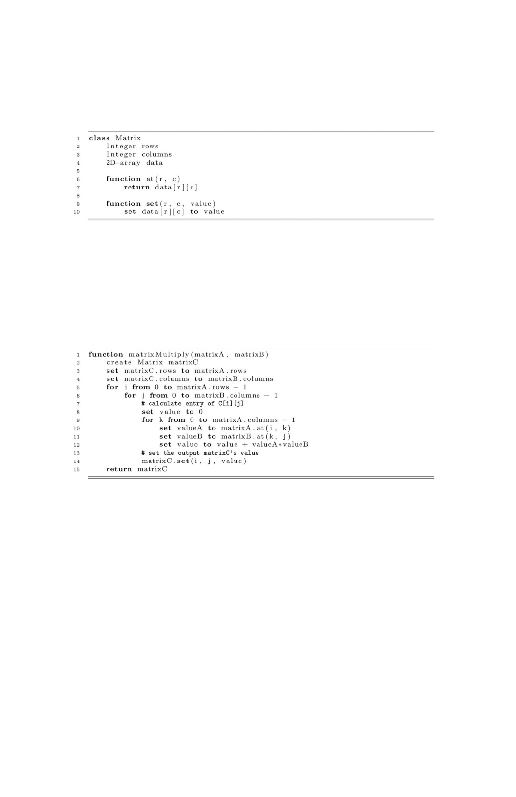
two convenience functions to access and set the values

of the matrix based on the row and column of the 2D

array.

With this structure for a Matrix class, we can

implement a matrix multiplication procedure. Below we

show the process of performing matrix multiplication on

two compatible matrices:

This function implements the matrix multiplication

procedure described above. On line 12, the new value of

the (i, j) entry in the result matrix is calculated. We see

that this involves a multiply operation and an addition

operation. On a typical processor, the multiply operation is

slower than addition. As we think about the complexity of

matrix multiplication, we will mainly consider the number

of multiplications. This is because as the matrices get

large, the cost associated with multiplication will dominate

the cost of addition. For this reason, we only consider the

number of multiplications.

So

how

many

multiplications

are

needed

for

matrix

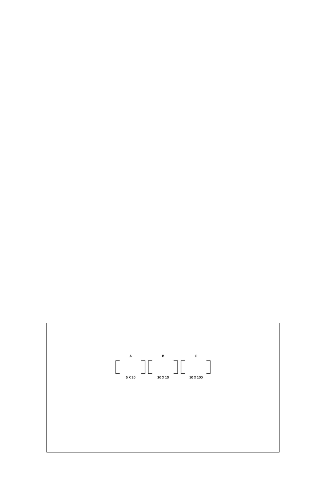
multiplication? The pattern above has a triple-nested loop.

This gives us a clue to the number of times the inner

code will run. As a result, we can expect the number of

multiplications to be equal to the number of times the

inner code will run. Let’s assume that matrix A has ra rows

and ca columns, and that matrix B, in a similar way, has rb

rows and cb columns. For A and B to be compatible

matrices, the value of ca would have to be equal to rb. We

know that the inner loop with index k runs a total of ca

times. This entire loop is executed once for every cb of B’s

columns (cb * ca). Finally, these two inner loops for j and k

would all run for every row in A, leading to multiplications

proportional to ra * ca * cb. This illustrates that as the size

of the matrices gets larger, the number of multiplications

grows quickly.

Why Order Matters

Now that we have seen how to multiply matrices together

and understand the computational cost, let’s consider just

why choosing to multiply in a specific order is important.

Suppose that we need to multiply three matrices—A, B,

and C—shown in the image below:

Figure 10.3

Multiplying them together could proceed with the

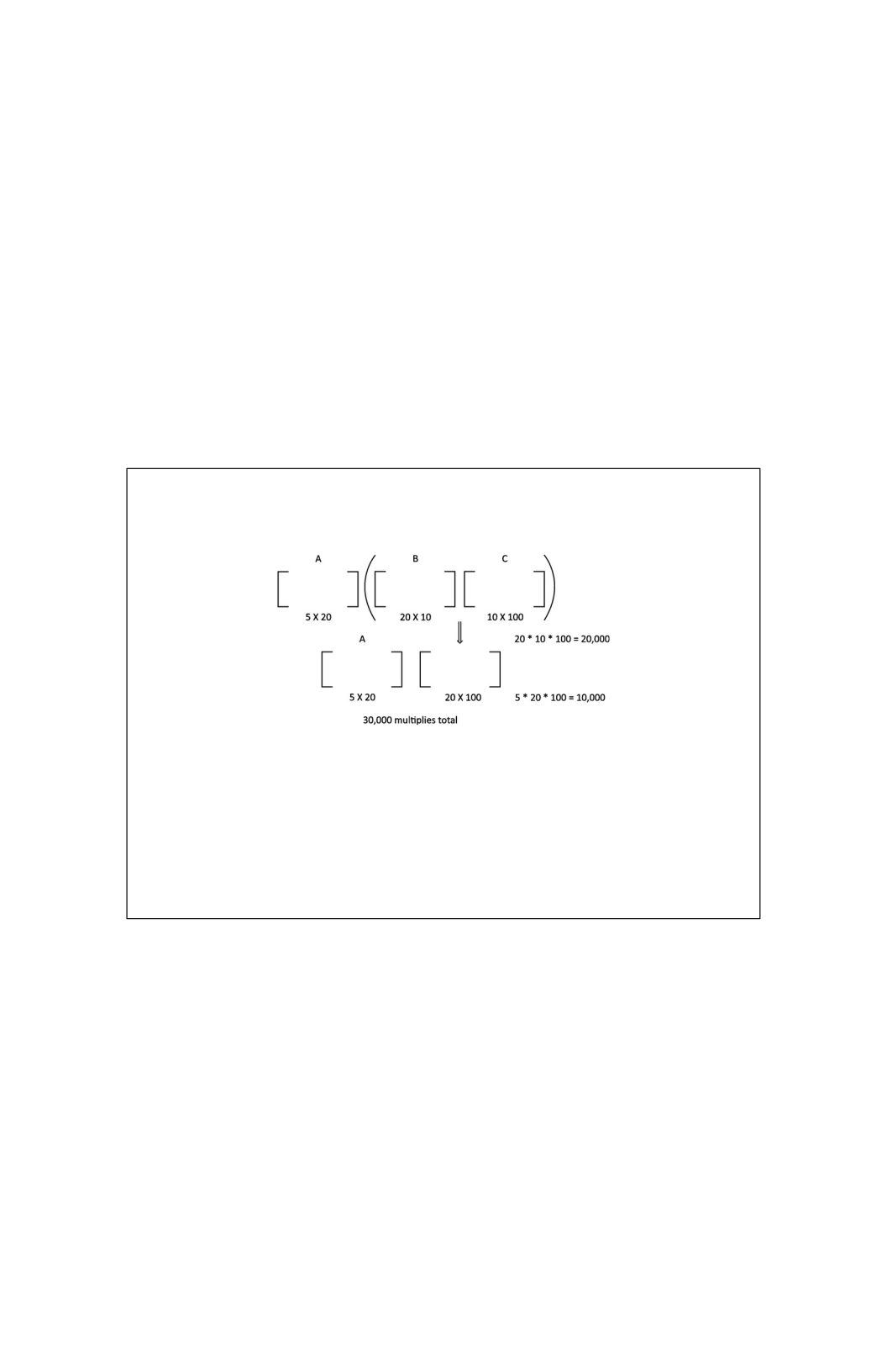
grouping (AB)C, where A and B are multiplied together

first, and then that result is multiplied by C. Alternatively, we

could group them as A(BC) and first multiply B by C, followed

by A multiplied by the result. Which would be better, or

would it even matter?

Let’s figure this out by first considering the A(BC)

grouping. The figure below illustrates this example. With

this grouping, calculating the BC multiplication yields

20,000 multiply operations. Multiplying A by this result

gives another 10,000 for a total of 30,000 multiply

operations.

Next, let’s consider the (AB)C grouping. The following

figure

shows a rough diagram of this calculation. The AB

matrix multiplication gives a cost of 1,000 multiply

operations. Then this result multiplied by C gives another

5,000. We now have a total of 6,000 multiply operations

for the (AB)C grouping over the other. This represents a

fivefold decrease in cost!

Figure 10.4

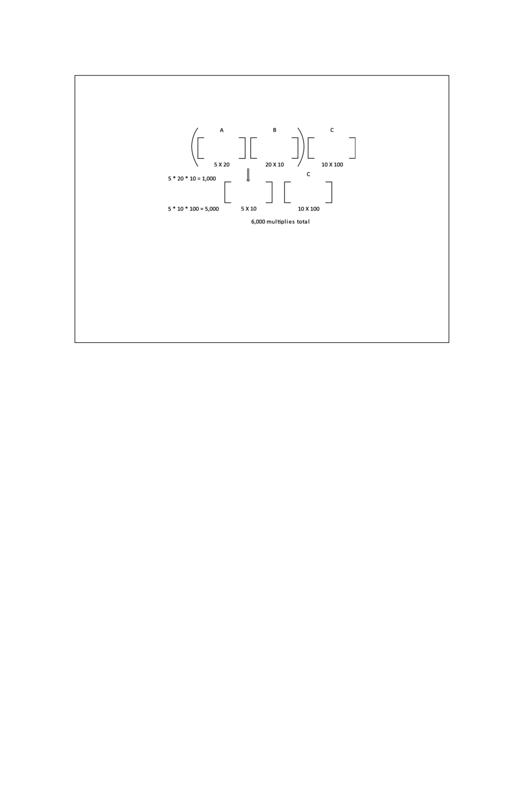
This example illustrates that the order of

multiplication definitely matters in terms of computational

cost. Additionally, as the matrices get larger, there could

be significant cost savings when we find an optimal

grouping for the multiplication sequence.

A Recursive Algorithm

for Optimal Matrix-Chain

Multiplication

We are interested in an algorithm for finding the optimal

ordering of matrix multiplication. This corresponds to

finding a grouping with a minimal cost. Suppose we have a

chain of 5 matrices, M

0

to M

4

. We could write their

dimensions as a list of 6 values. The 6 values come from

the fact that each sequential pair of matrices must be

compatible for multiplication to be possible. The figure

below shows this chain and gives the dimensions as a list.

Figure 10.5

An algorithm that minimizes the cost must find an

optimal split for the final two matrices. Let’s call these final

two matrices A and B. For the result to be optimal, then A

and B must both have resulted from an optimal subgrouping.

The possible splits would be

We need to evaluate these options by assessing

the cost of creating the A and B matrices (optimal

subproblems) as well as the cost of the final multiply, with

matrix A being multiplied by B. A recursive algorithm

would find the minimal cost by checking the minimum cost

among all splits. In the process of finding the cost of all

these four options for splits, we would need to calculate

the optimal splits for other sequences to find their optimal

groupings. This demonstrates the feature of optimal

substructure, the idea that an optimal solution could be

Figure 10.6

(M0) (M1 M2 M3 M4) = AB with a split after

position 0 (M0 M1) (M2 M3 M4) = AB with a split

after position 1 (M0 M1 M2) (M3 M4) = AB with a

split after position 2 (M0 M1 M2 M3) (M4) = AB

with a split after position 3.

built from optimal subproblems.

For the first grouping, we have A = M0 and B = (M1

M2 M3 M

4

). To calculate the cost of this split, it is

assumed that A and B have been constructed optimally.

This means that a recursive algorithm considering this split

must then make a recursive call to

find the minimal

grouping for (M1 M2 M3 M4) for the B matrix. This in

turn

would trigger another search for the optimal split among

(M

1

) (M2 M3 M4) (M1 M2) (M3 M4) and (M1 M2 M3) (M4). We

can also see

that this would trigger further calls to optimize each

sequence of 3 matrices and so on. You may be able to

imagine that this recursive process has a high branch

factor leading to an exponential runtime complexity in the

number of matrices. With n matrices, the runtime

complexity would be even worse than O(2n), exponential time. It

would follow an algorithm for calculating the Catalan

numbers at O(3n).

A general outline of the recursive algorithm would be

as follows. We will consider an algorithm to calculate the

minimal cost of multiplying a sequence of matrices starting at

some matrix identified by the start index and including the

ending matrix using an end index. The base case of the

algorithm is when start and end are equal. The cost of

multiplication of only one matrix is 0 as there is no

operation to perform. The recursive case calculates the cost

of splitting the sequence at some split position. There will be

n − 1 split positions to test when considering n matrices

where n = end − start

+ 1, and the recursive algorithm will need to find the

minimum of the options for the best split position.

To complete the recursive algorithm, we will

introduce a function to calculate the cost of the final

multiplication. This could be a simple multiplication of the

correct dimensions, but we will introduce and explain this

function to make the meaning clear and to simplify some

of the code (which would otherwise include a lot of

awkward indexing). The figure below illustrates what is

meant by the final multiplication:

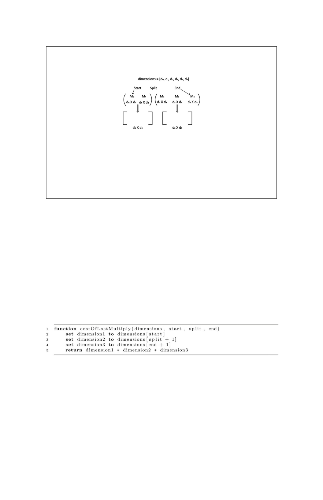
Suppose we are calculating the number of

multiplications for a split at index 1 (or just after M1). The

algorithm would have given the optimal cost for constructing

the left matrix and the right matrix, but we would still need to

calculate the cost of multiplying those together. The left

matrix would have dimensions of d0 by d2 and the right

matrix would have dimensions of d2 by d5. Using the

dimensions list and indexes for start, split, and end, we can

calculate this cost. The function below performs this operation

in a way that might make the meaning a little clearer. Notice

that for matrix i, the dimensions of that matrix are di by di+1.

With this helper function, we can now write the

recursive algorithm.

Figure 10.7

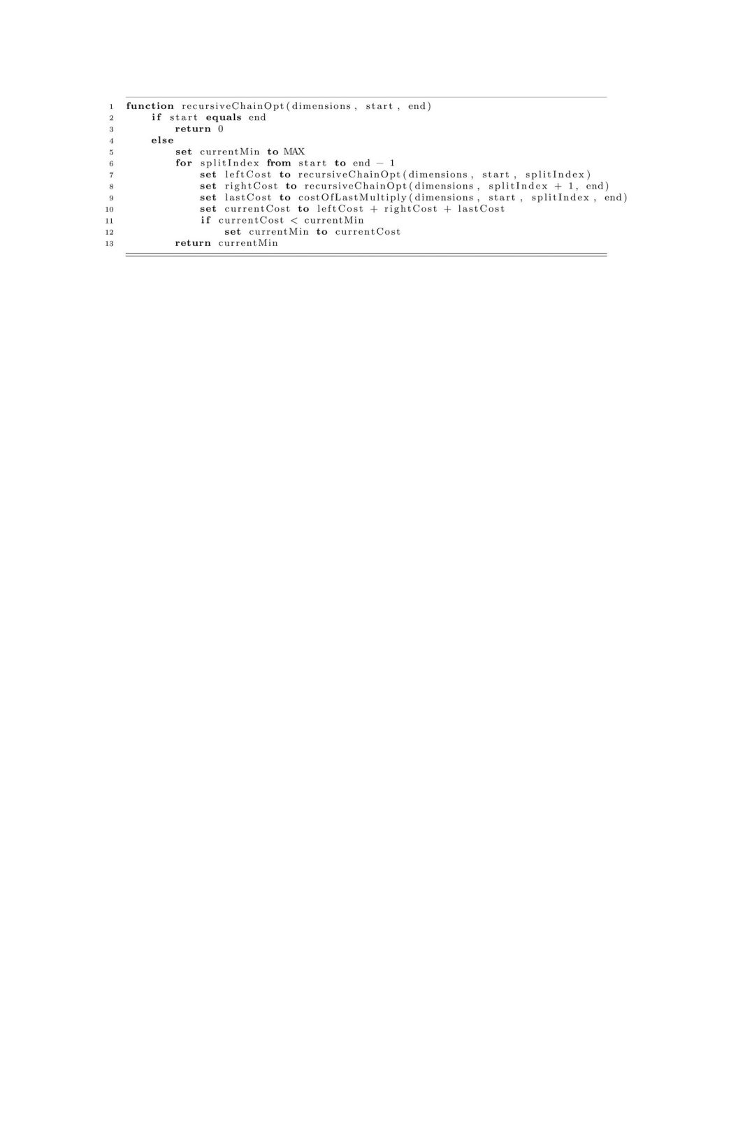
This algorithm only calculates an optimal cost, but

it could be modified to record the split indexes of the

optimal splits so that another process could use that

information. The optimal cost of multiplying all matrices in

the optimal grouping could be calculated with a call to

recursiveChainOpt(dimensions, 0, 4). This algorithm, while

correct, suffers from exponential time complexity. This is

the type of situation where dynamic programming can

help.

Requirements for Applying

Dynamic Programming

There are two main requirements for applying dynamic

programming. First, a problem must exhibit the property

known as optimal substructure. This means that an

optimal solution to the problem is constructed from

optimal solutions to the subproblems. We will see an

example of this soon. The second property is called

overlapping subproblems. This means that subproblems

are shared. We saw this in our Fibonacci example.

Optimal Matrix Chain Multiplication

A classic application of dynamic programming concerns

the optimal multiplication order for matrices. Consider the

sequence of matrices {M1, M2, M3, M4}. There are several

ways to multiply these together. These ways correspond

to the number of distinct ways to parenthesize the matrix

multiplication order. For the mathematically curious, the

Catalan numbers give the total number of possible ways.

For example, one way to group these would be (M

1

M2) (M3

M4). Another way could be M1 ((M2 M3) M4). Any grouping

leads to the same final result, but the number of multiply

operations of the overall calculation could differ greatly

with different groupings. To understand this idea, let’s

review matrix multiplication.

Matrix

Multiplication

Review

Matrix multiplication is an operation that multiplies and adds the

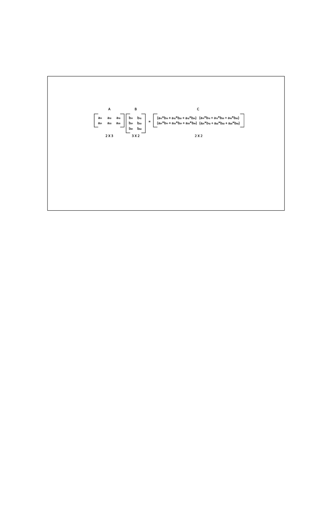
rows of one matrix with the columns of another matrix.

Below is an example:

Here we have the matrix A and the matrix B. A is a

2-by-3 matrix (2 rows and 3 columns), and B is a 3-by-2

matrix (3 rows

and 2 columns). The multiplication of AB is

compatible, which means

the number of columns of A is

equal to the number of rows in the second matrix, B. When

two compatible matrices are multiplied, their result has a

structure where the number of rows equals the number of

rows in the first matrix and the number of columns equals

the number of columns in the second matrix. The process

is the same for compatible matrices of any size.

Implementing

Matrix

Multiplication

Now let’s consider an algorithm for matrix multiplication.

To simplify things, let’s assume we have a Matrix class or

data structure that has a two-dimensional (2D) array.

Another way to think of a 2D array is as an array of

arrays. We could also think of this as a table with rows

and columns. The structure below gives a general example

of a Matrix class. Within this class, we also have

Figure 10.2

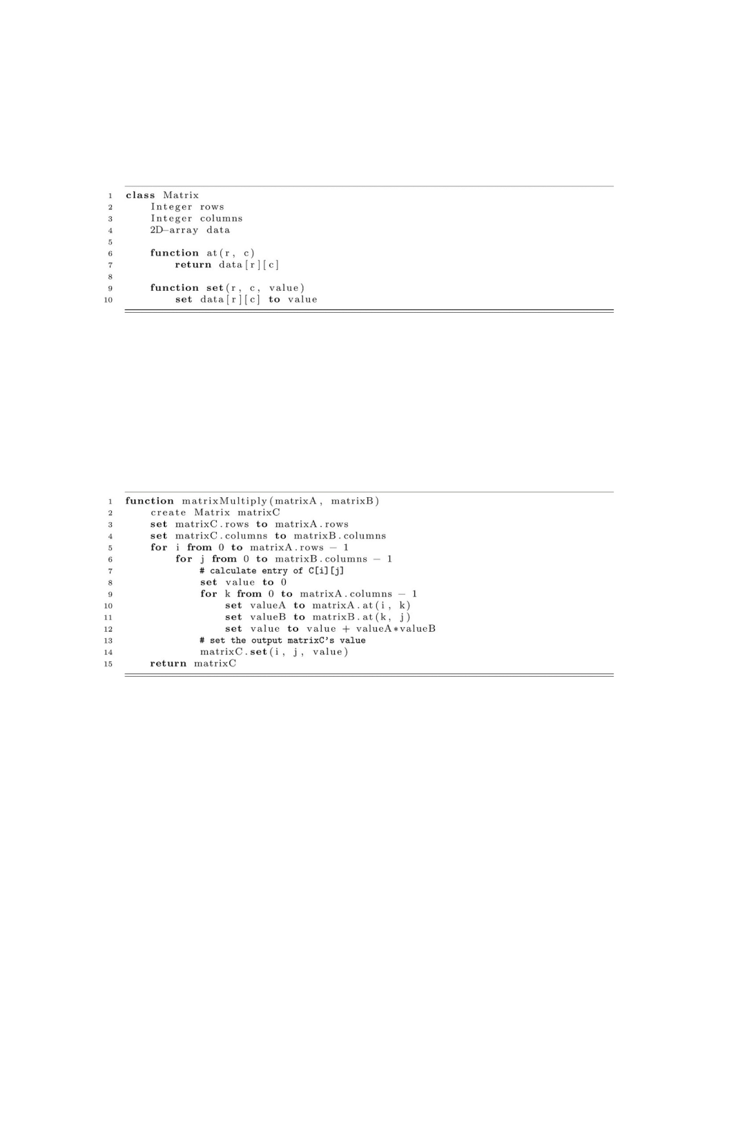
two convenience functions to access and set the values

of the matrix based on the row and column of the 2D

array.

With this structure for a Matrix class, we can

implement a matrix multiplication procedure. Below we

show the process of performing matrix multiplication on

two compatible matrices:

This function implements the matrix multiplication

procedure described above. On line 12, the new value of

the (i, j) entry in the result matrix is calculated. We see

that this involves a multiply operation and an addition

operation. On a typical processor, the multiply operation is

slower than addition. As we think about the complexity of

matrix multiplication, we will mainly consider the number

of multiplications. This is because as the matrices get

large, the cost associated with multiplication will dominate

the cost of addition. For this reason, we only consider the

number of multiplications.

So

how

many

multiplications

are

needed

for

matrix

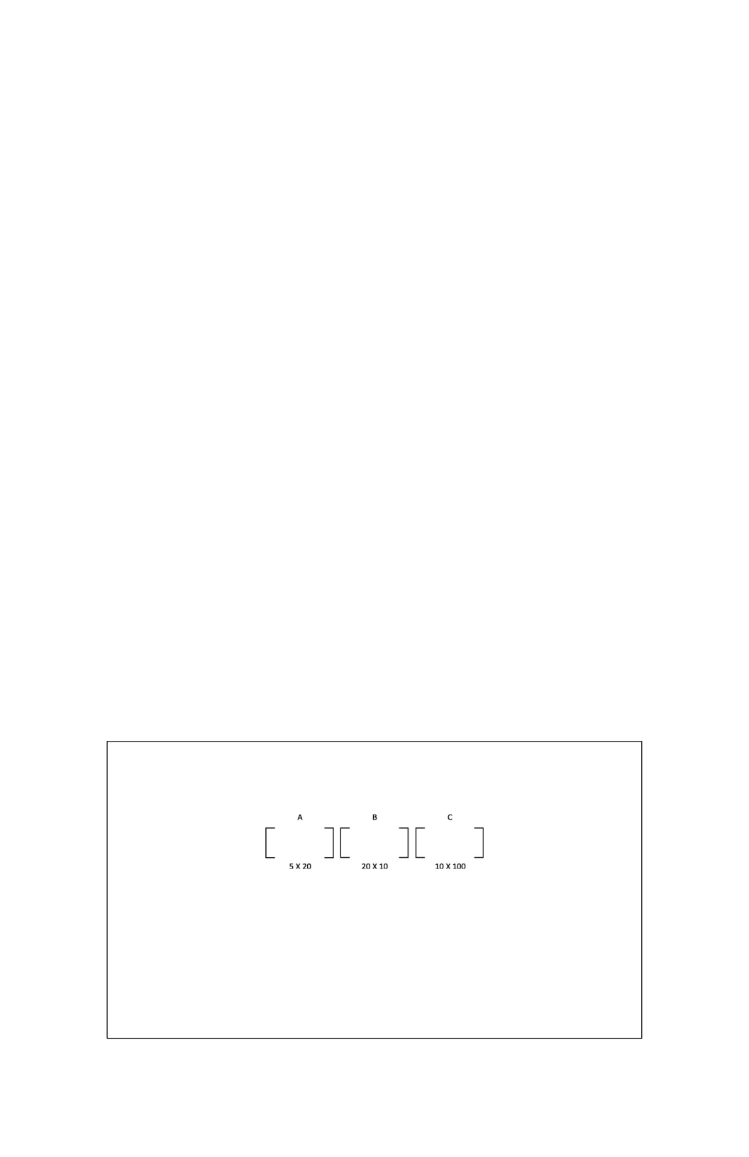
multiplication? The pattern above has a triple-nested loop.

This gives us a clue to the number of times the inner

code will run. As a result, we can expect the number of

multiplications to be equal to the number of times the

inner code will run. Let’s assume that matrix A has ra rows

and ca columns, and that matrix B, in a similar way, has rb

rows and cb columns. For A and B to be compatible

matrices, the value of ca would have to be equal to rb. We

know that the inner loop with index k runs a total of ca

times. This entire loop is executed once for every cb of B’s

columns (cb * ca). Finally, these two inner loops for j and k

would all run for every row in A, leading to multiplications

proportional to ra * ca * cb. This illustrates that as the size

of the matrices gets larger, the number of multiplications

grows quickly.

Why Order Matters

Now that we have seen how to multiply matrices together

and understand the computational cost, let’s consider just

why choosing to multiply in a specific order is important.

Suppose that we need to multiply three matrices—A, B,

and C—shown in the image below:

Figure 10.3

Multiplying them together could proceed with the

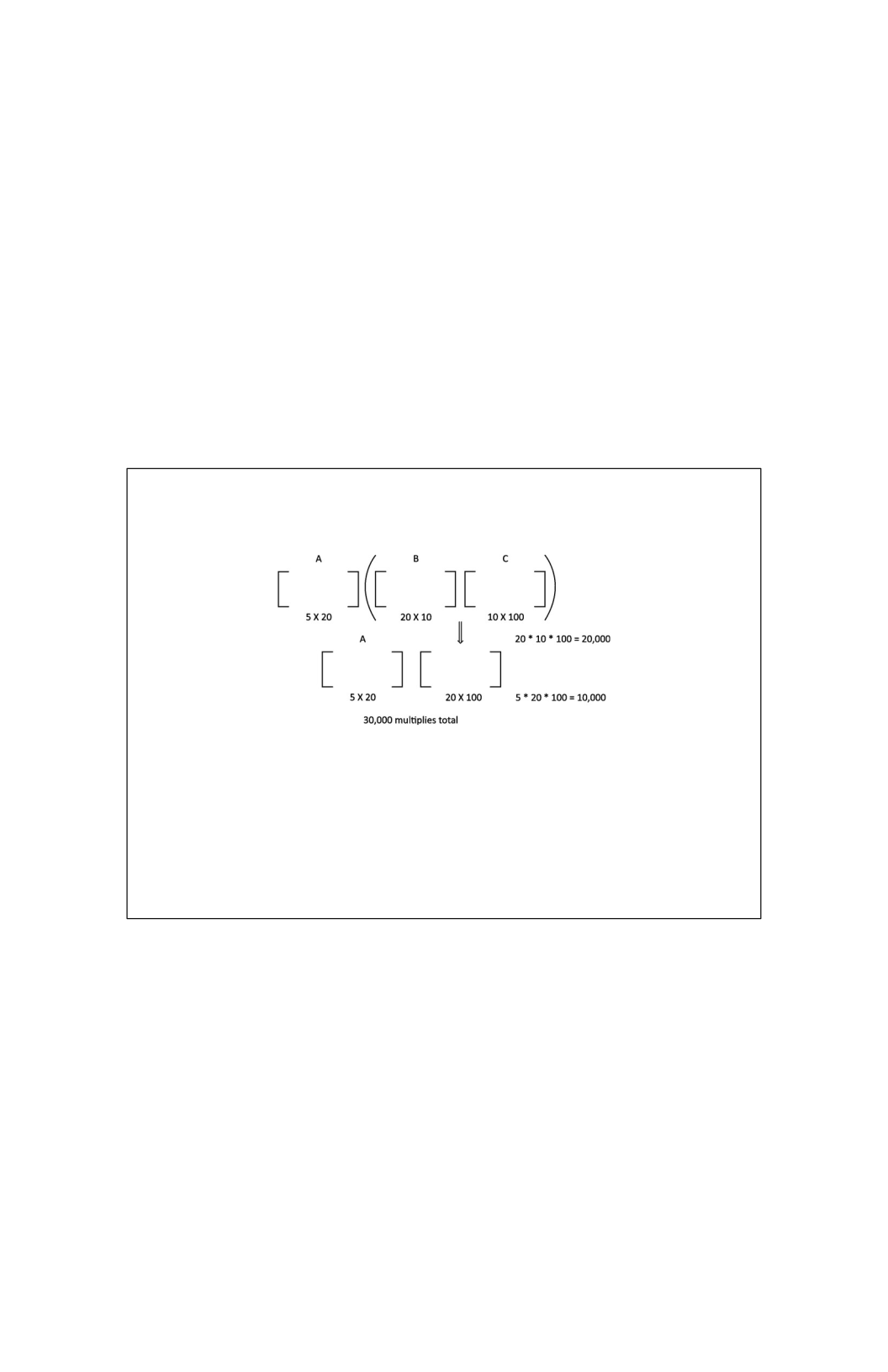
grouping (AB)C, where A and B are multiplied together

first, and then that result is multiplied by C. Alternatively, we

could group them as A(BC) and first multiply B by C, followed

by A multiplied by the result. Which would be better, or

would it even matter?

Let’s figure this out by first considering the A(BC)

grouping. The figure below illustrates this example. With

this grouping, calculating the BC multiplication yields

20,000 multiply operations. Multiplying A by this result

gives another 10,000 for a total of 30,000 multiply

operations.

Next, let’s consider the (AB)C grouping. The following

figure

shows a rough diagram of this calculation. The AB

matrix multiplication gives a cost of 1,000 multiply

operations. Then this result multiplied by C gives another

5,000. We now have a total of 6,000 multiply operations

for the (AB)C grouping over the other. This represents a

fivefold decrease in cost!

Figure 10.4

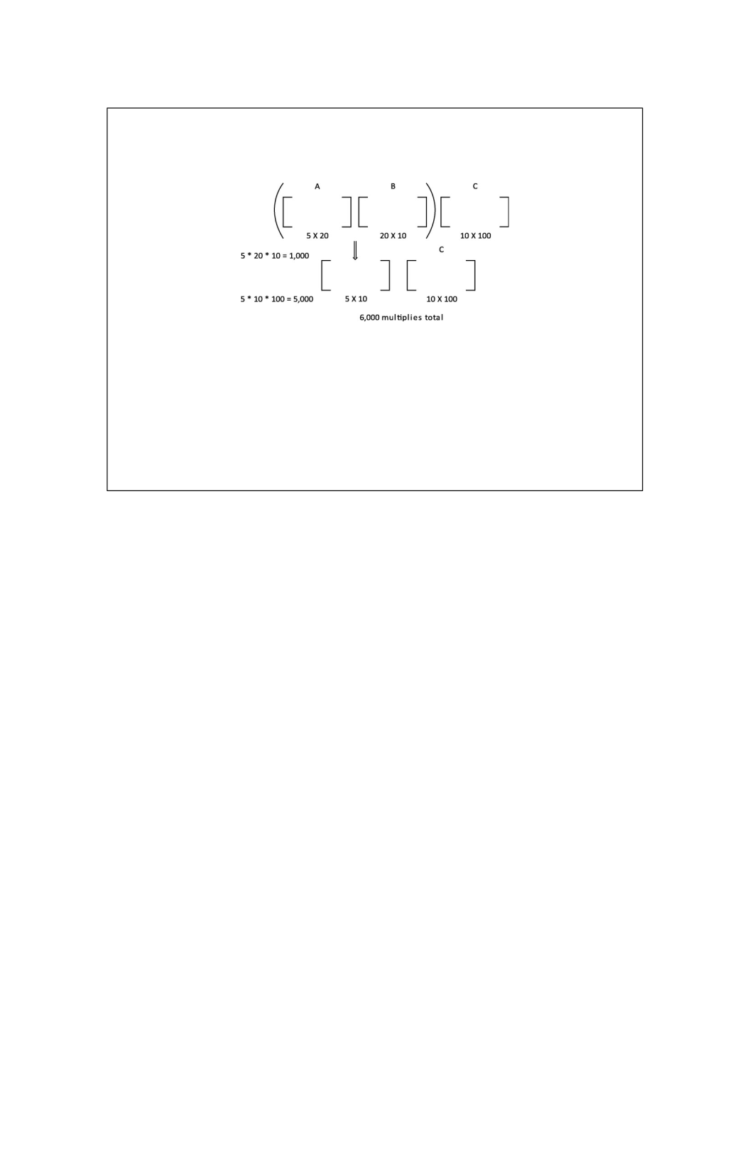
This example illustrates that the order of

multiplication definitely matters in terms of computational

cost. Additionally, as the matrices get larger, there could

be significant cost savings when we find an optimal

grouping for the multiplication sequence.

A Recursive Algorithm

for Optimal Matrix-Chain

Multiplication

We are interested in an algorithm for finding the optimal

ordering of matrix multiplication. This corresponds to

finding a grouping with a minimal cost. Suppose we have a

chain of 5 matrices, M

0

to M

4

. We could write their

dimensions as a list of 6 values. The 6 values come from

the fact that each sequential pair of matrices must be

compatible for multiplication to be possible. The figure

below shows this chain and gives the dimensions as a list.

Figure 10.5

An algorithm that minimizes the cost must find an

optimal split for the final two matrices. Let’s call these final

two matrices A and B. For the result to be optimal, then A

and B must both have resulted from an optimal subgrouping.

The possible splits would be

We need to evaluate these options by assessing

the cost of creating the A and B matrices (optimal

subproblems) as well as the cost of the final multiply, with

matrix A being multiplied by B. A recursive algorithm

would find the minimal cost by checking the minimum cost

among all splits. In the process of finding the cost of all

these four options for splits, we would need to calculate

the optimal splits for other sequences to find their optimal

groupings. This demonstrates the feature of optimal

substructure, the idea that an optimal solution could be

Figure 10.6

(M0) (M1 M2 M3 M4) = AB with a split after

position 0 (M0 M1) (M2 M3 M4) = AB with a split

after position 1 (M0 M1 M2) (M3 M4) = AB with a

split after position 2 (M0 M1 M2 M3) (M4) = AB

with a split after position 3.

built from optimal subproblems.

For the first grouping, we have A = M0 and B = (M1

M2 M3 M

4

). To calculate the cost of this split, it is

assumed that A and B have been constructed optimally.

This means that a recursive algorithm considering this split

must then make a recursive call to

find the minimal

grouping for (M1 M2 M3 M4) for the B matrix. This in

turn

would trigger another search for the optimal split among

(M

1

) (M2 M3 M4) (M1 M2) (M3 M4) and (M1 M2 M3) (M4). We

can also see

that this would trigger further calls to optimize each

sequence of 3 matrices and so on. You may be able to

imagine that this recursive process has a high branch

factor leading to an exponential runtime complexity in the

number of matrices. With n matrices, the runtime

complexity would be even worse than O(2n), exponential time. It

would follow an algorithm for calculating the Catalan

numbers at O(3n).

A general outline of the recursive algorithm would be

as follows. We will consider an algorithm to calculate the

minimal cost of multiplying a sequence of matrices starting at

some matrix identified by the start index and including the

ending matrix using an end index. The base case of the

algorithm is when start and end are equal. The cost of

multiplication of only one matrix is 0 as there is no

operation to perform. The recursive case calculates the cost

of splitting the sequence at some split position. There will be

n − 1 split positions to test when considering n matrices

where n = end − start

+ 1, and the recursive algorithm will need to find the

minimum of the options for the best split position.

To complete the recursive algorithm, we will

introduce a function to calculate the cost of the final

multiplication. This could be a simple multiplication of the

correct dimensions, but we will introduce and explain this

function to make the meaning clear and to simplify some

of the code (which would otherwise include a lot of

awkward indexing). The figure below illustrates what is

meant by the final multiplication:

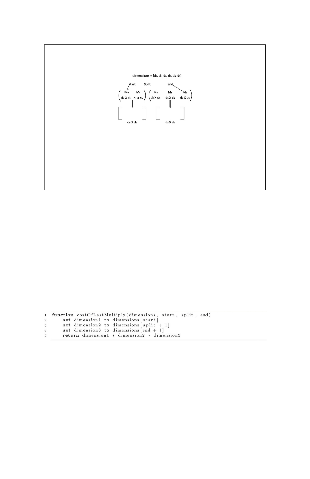
Suppose we are calculating the number of

multiplications for a split at index 1 (or just after M1). The

algorithm would have given the optimal cost for constructing

the left matrix and the right matrix, but we would still need to

calculate the cost of multiplying those together. The left

matrix would have dimensions of d0 by d2 and the right

matrix would have dimensions of d2 by d5. Using the

dimensions list and indexes for start, split, and end, we can

calculate this cost. The function below performs this operation

in a way that might make the meaning a little clearer. Notice

that for matrix i, the dimensions of that matrix are di by di+1.

With this helper function, we can now write the

recursive algorithm.

Figure 10.7

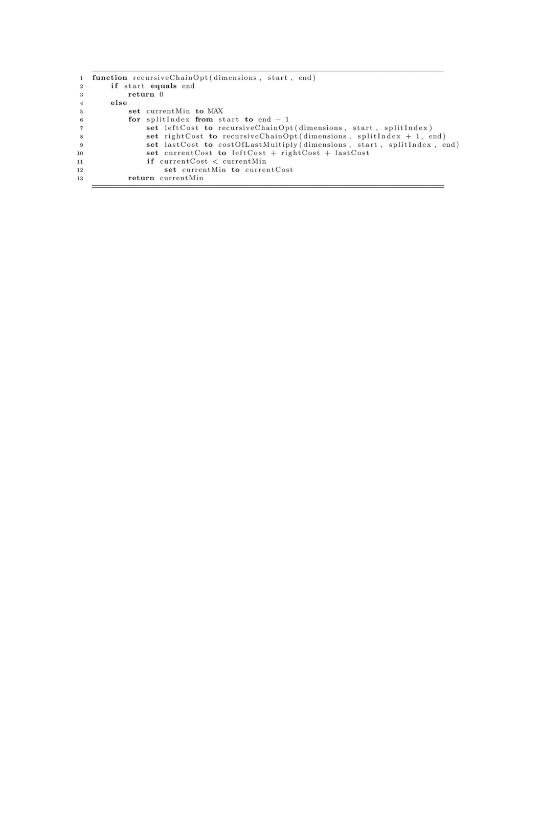
This algorithm only calculates an optimal cost, but

it could be modified to record the split indexes of the

optimal splits so that another process could use that

information. The optimal cost of multiplying all matrices in

the optimal grouping could be calculated with a call to

recursiveChainOpt(dimensions, 0, 4). This algorithm, while

correct, suffers from exponential time complexity. This is

the type of situation where dynamic programming can

help.

Requirements for Applying

Dynamic Programming

There are two main requirements for applying dynamic

programming. First, a problem must exhibit the property

known as optimal substructure. This means that an

optimal solution to the problem is constructed from

optimal solutions to the subproblems. We will see an

example of this soon. The second property is called

overlapping subproblems. This means that subproblems

are shared. We saw this in our Fibonacci example.

Optimal Matrix Chain Multiplication

A classic application of dynamic programming concerns

the optimal multiplication order for matrices. Consider the

sequence of matrices {M1, M2, M3, M4}. There are several

ways to multiply these together. These ways correspond

to the number of distinct ways to parenthesize the matrix

multiplication order. For the mathematically curious, the

Catalan numbers give the total number of possible ways.

For example, one way to group these would be (M

1

M2) (M3

M4). Another way could be M1 ((M2 M3) M4). Any grouping

leads to the same final result, but the number of multiply

operations of the overall calculation could differ greatly

with different groupings. To understand this idea, let’s

review matrix multiplication.

Matrix

Multiplication

Review

Matrix multiplication is an operation that multiplies and adds the

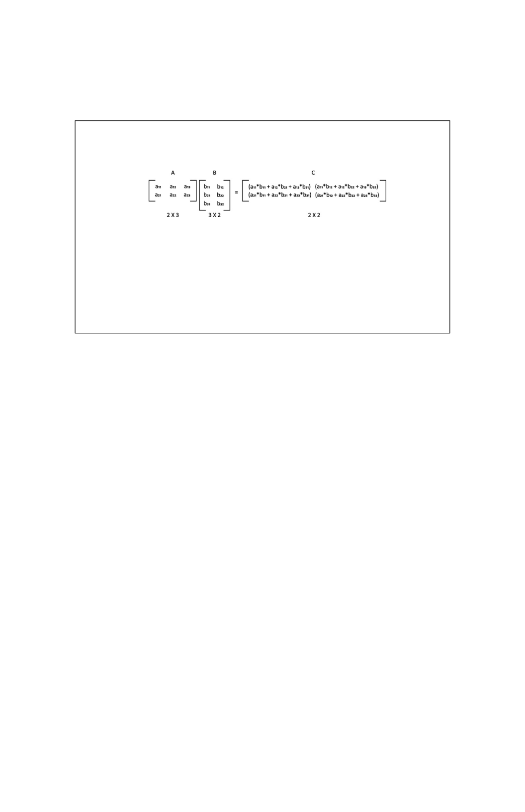
rows of one matrix with the columns of another matrix.

Below is an example:

Here we have the matrix A and the matrix B. A is a

2-by-3 matrix (2 rows and 3 columns), and B is a 3-by-2

matrix (3 rows

and 2 columns). The multiplication of AB is

compatible, which means

the number of columns of A is

equal to the number of rows in the second matrix, B. When

two compatible matrices are multiplied, their result has a

structure where the number of rows equals the number of

rows in the first matrix and the number of columns equals

the number of columns in the second matrix. The process

is the same for compatible matrices of any size.

Implementing

Matrix

Multiplication

Now let’s consider an algorithm for matrix multiplication.

To simplify things, let’s assume we have a Matrix class or

data structure that has a two-dimensional (2D) array.

Another way to think of a 2D array is as an array of

arrays. We could also think of this as a table with rows

and columns. The structure below gives a general example

of a Matrix class. Within this class, we also have

Figure 10.2

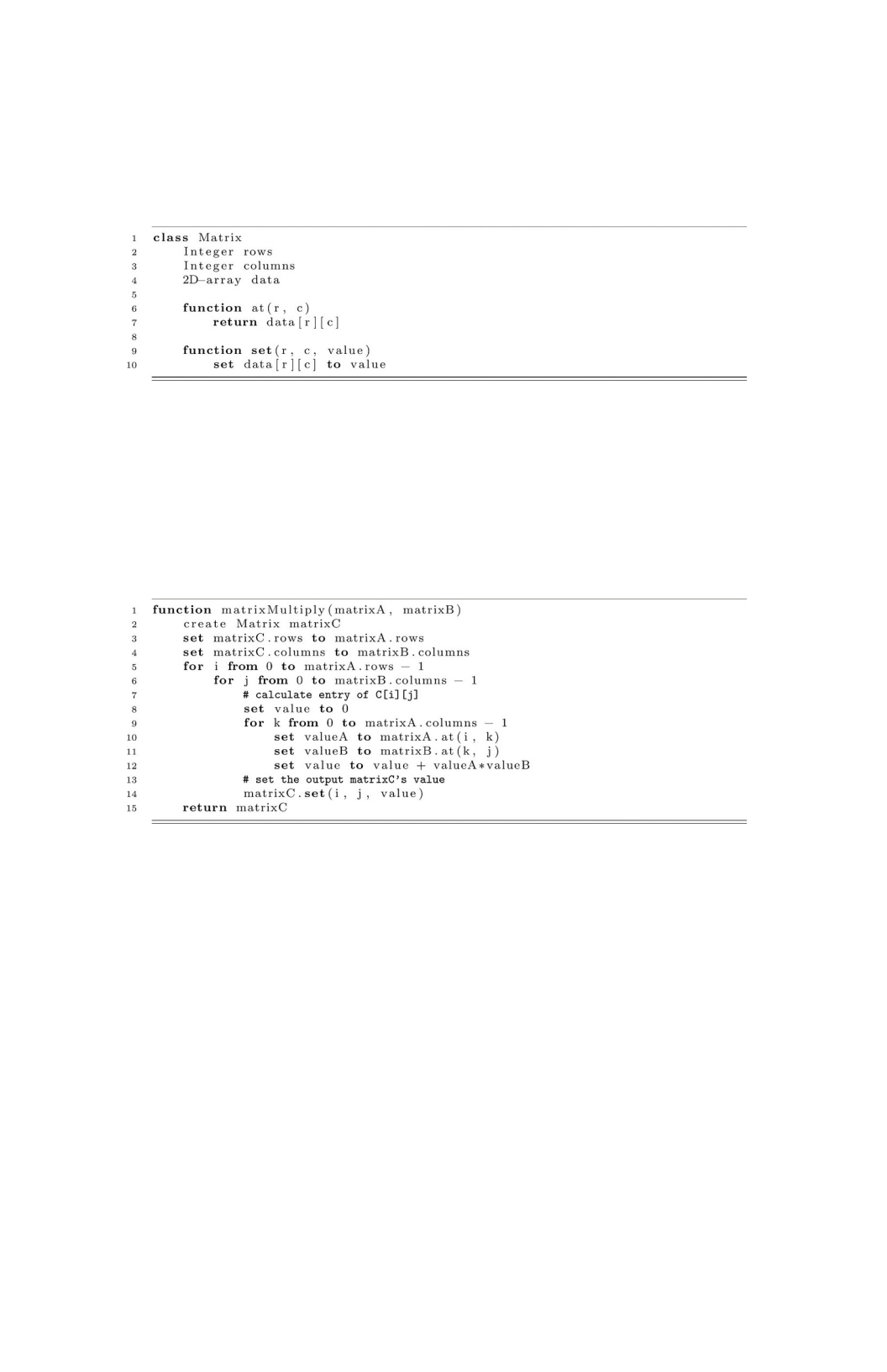
two convenience functions to access and set the values

of the matrix based on the row and column of the 2D

array.

With this structure for a Matrix class, we can

implement a matrix multiplication procedure. Below we

show the process of performing matrix multiplication on

two compatible matrices:

This function implements the matrix multiplication

procedure described above. On line 12, the new value of

the (i, j) entry in the result matrix is calculated. We see

that this involves a multiply operation and an addition

operation. On a typical processor, the multiply operation is

slower than addition. As we think about the complexity of

matrix multiplication, we will mainly consider the number

of multiplications. This is because as the matrices get

large, the cost associated with multiplication will dominate

the cost of addition. For this reason, we only consider the

number of multiplications.

So

how

many

multiplications

are

needed

for

matrix

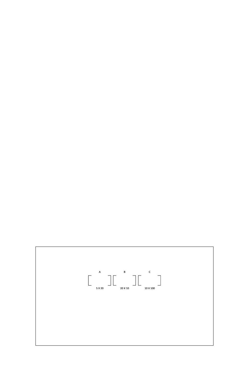
multiplication? The pattern above has a triple-nested loop.

This gives us a clue to the number of times the inner

code will run. As a result, we can expect the number of

multiplications to be equal to the number of times the

inner code will run. Let’s assume that matrix A has ra rows

and ca columns, and that matrix B, in a similar way, has rb

rows and cb columns. For A and B to be compatible

matrices, the value of ca would have to be equal to rb. We

know that the inner loop with index k runs a total of ca

times. This entire loop is executed once for every cb of B’s

columns (cb * ca). Finally, these two inner loops for j and k

would all run for every row in A, leading to multiplications

proportional to ra * ca * cb. This illustrates that as the size

of the matrices gets larger, the number of multiplications

grows quickly.

Why Order Matters

Now that we have seen how to multiply matrices together

and understand the computational cost, let’s consider just

why choosing to multiply in a specific order is important.

Suppose that we need to multiply three matrices—A, B,

and C—shown in the image below:

Figure 10.3

Multiplying them together could proceed with the

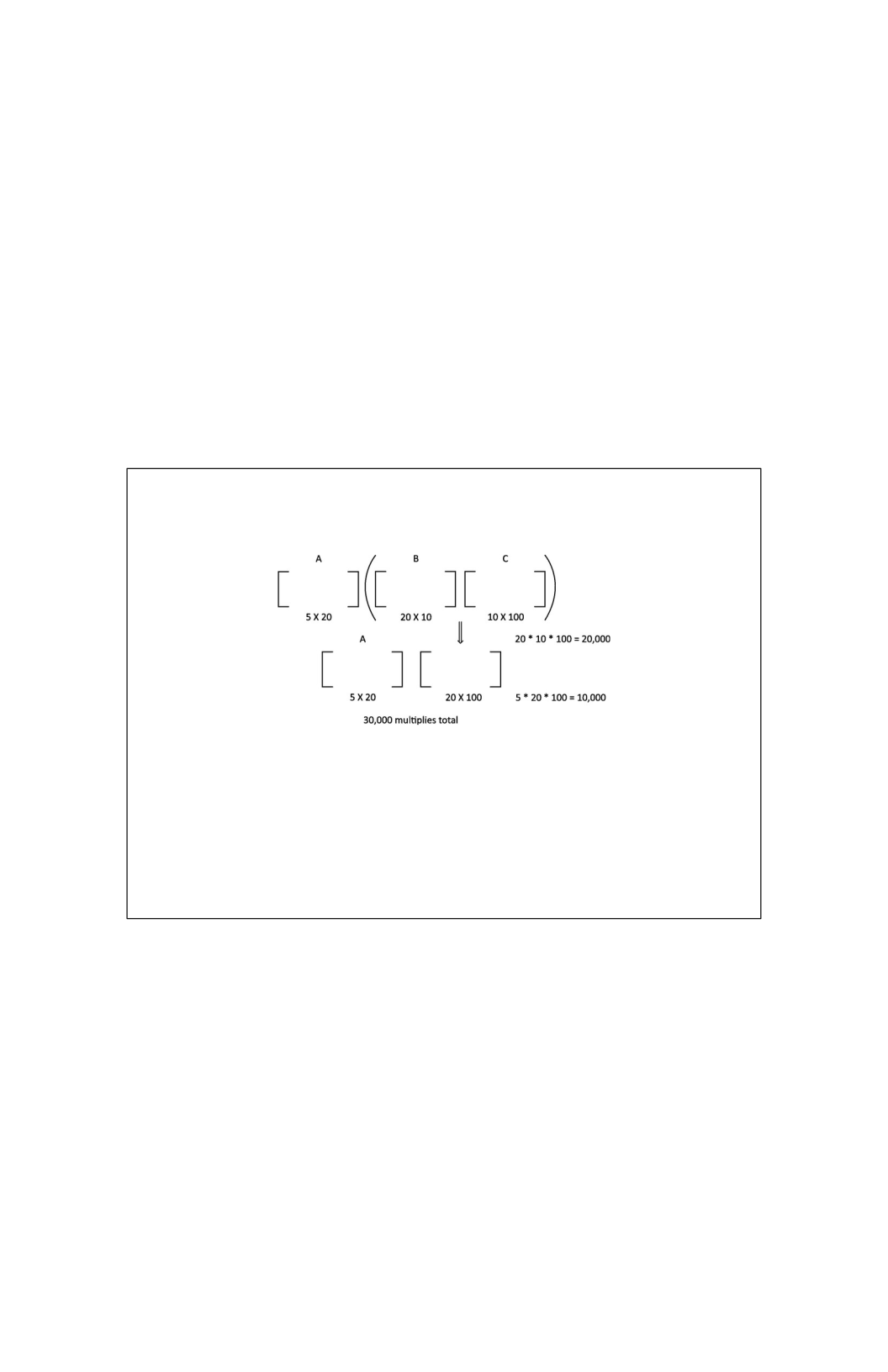
grouping (AB)C, where A and B are multiplied together

first, and then that result is multiplied by C. Alternatively, we

could group them as A(BC) and first multiply B by C, followed

by A multiplied by the result. Which would be better, or

would it even matter?

Let’s figure this out by first considering the A(BC)

grouping. The figure below illustrates this example. With

this grouping, calculating the BC multiplication yields

20,000 multiply operations. Multiplying A by this result

gives another 10,000 for a total of 30,000 multiply

operations.

Next, let’s consider the (AB)C grouping. The following

figure

shows a rough diagram of this calculation. The AB

matrix multiplication gives a cost of 1,000 multiply

operations. Then this result multiplied by C gives another

5,000. We now have a total of 6,000 multiply operations

for the (AB)C grouping over the other. This represents a

fivefold decrease in cost!

Figure 10.4

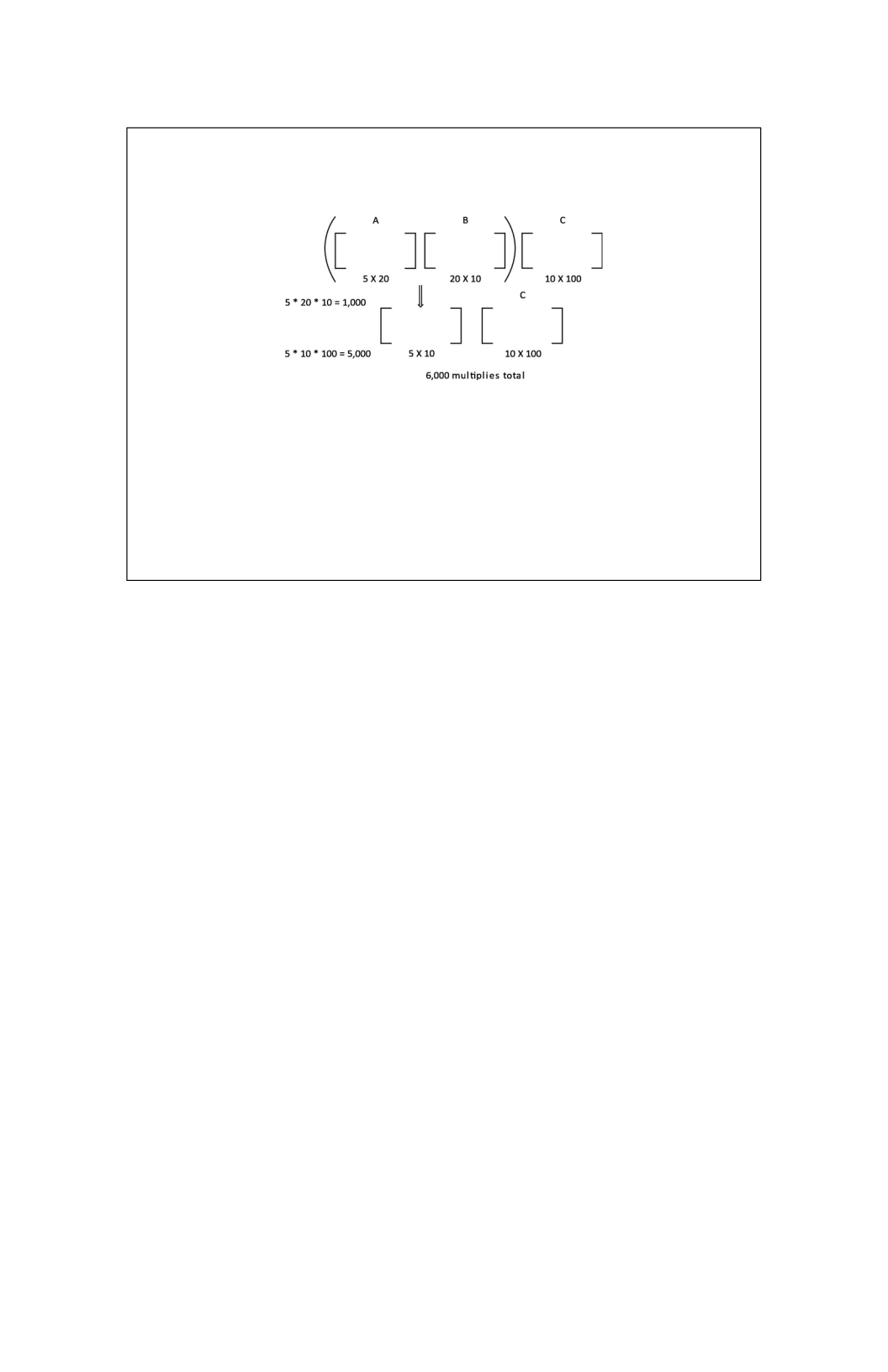
This example illustrates that the order of

multiplication definitely matters in terms of computational

cost. Additionally, as the matrices get larger, there could

be significant cost savings when we find an optimal

grouping for the multiplication sequence.

A Recursive Algorithm

for Optimal Matrix-Chain

Multiplication

We are interested in an algorithm for finding the optimal

ordering of matrix multiplication. This corresponds to

finding a grouping with a minimal cost. Suppose we have a

chain of 5 matrices, M

0

to M

4

. We could write their

dimensions as a list of 6 values. The 6 values come from

the fact that each sequential pair of matrices must be

compatible for multiplication to be possible. The figure

below shows this chain and gives the dimensions as a list.

Figure 10.5

An algorithm that minimizes the cost must find an

optimal split for the final two matrices. Let’s call these final

two matrices A and B. For the result to be optimal, then A

and B must both have resulted from an optimal subgrouping.

The possible splits would be

We need to evaluate these options by assessing

the cost of creating the A and B matrices (optimal

subproblems) as well as the cost of the final multiply, with

matrix A being multiplied by B. A recursive algorithm

would find the minimal cost by checking the minimum cost

among all splits. In the process of finding the cost of all

these four options for splits, we would need to calculate

the optimal splits for other sequences to find their optimal

groupings. This demonstrates the feature of optimal

substructure, the idea that an optimal solution could be

Figure 10.6

(M0) (M1 M2 M3 M4) = AB with a split after

position 0 (M0 M1) (M2 M3 M4) = AB with a split

after position 1 (M0 M1 M2) (M3 M4) = AB with a

split after position 2 (M0 M1 M2 M3) (M4) = AB

with a split after position 3.

built from optimal subproblems.

For the first grouping, we have A = M0 and B = (M1

M2 M3 M

4

). To calculate the cost of this split, it is

assumed that A and B have been constructed optimally.

This means that a recursive algorithm considering this split

must then make a recursive call to

find the minimal

grouping for (M1 M2 M3 M4) for the B matrix. This in

turn

would trigger another search for the optimal split among

(M

1

) (M2 M3 M4) (M1 M2) (M3 M4) and (M1 M2 M3) (M4). We

can also see

that this would trigger further calls to optimize each

sequence of 3 matrices and so on. You may be able to

imagine that this recursive process has a high branch

factor leading to an exponential runtime complexity in the

number of matrices. With n matrices, the runtime

complexity would be even worse than O(2n), exponential time. It

would follow an algorithm for calculating the Catalan

numbers at O(3n).

A general outline of the recursive algorithm would be

as follows. We will consider an algorithm to calculate the

minimal cost of multiplying a sequence of matrices starting at

some matrix identified by the start index and including the

ending matrix using an end index. The base case of the

algorithm is when start and end are equal. The cost of

multiplication of only one matrix is 0 as there is no

operation to perform. The recursive case calculates the cost

of splitting the sequence at some split position. There will be

n − 1 split positions to test when considering n matrices

where n = end − start

+ 1, and the recursive algorithm will need to find the

minimum of the options for the best split position.

To complete the recursive algorithm, we will

introduce a function to calculate the cost of the final

multiplication. This could be a simple multiplication of the

correct dimensions, but we will introduce and explain this

function to make the meaning clear and to simplify some

of the code (which would otherwise include a lot of

awkward indexing). The figure below illustrates what is

meant by the final multiplication:

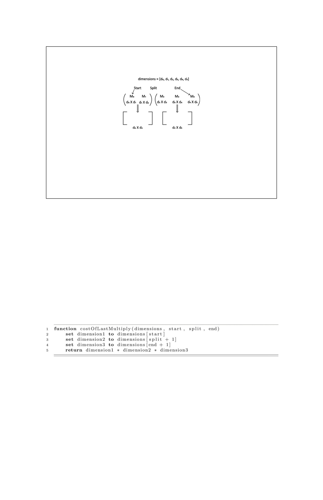
Suppose we are calculating the number of

multiplications for a split at index 1 (or just after M1). The

algorithm would have given the optimal cost for constructing

the left matrix and the right matrix, but we would still need to

calculate the cost of multiplying those together. The left

matrix would have dimensions of d0 by d2 and the right

matrix would have dimensions of d2 by d5. Using the

dimensions list and indexes for start, split, and end, we can

calculate this cost. The function below performs this operation

in a way that might make the meaning a little clearer. Notice

that for matrix i, the dimensions of that matrix are di by di+1.

With this helper function, we can now write the

recursive algorithm.

Figure 10.7

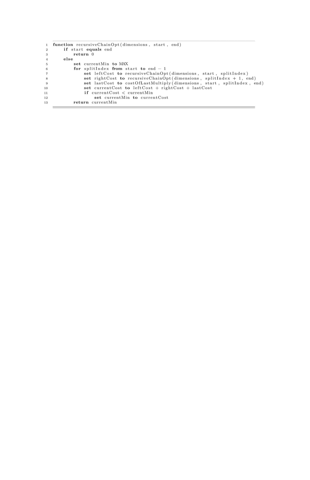
This algorithm only calculates an optimal cost, but

it could be modified to record the split indexes of the

optimal splits so that another process could use that

information. The optimal cost of multiplying all matrices in

the optimal grouping could be calculated with a call to

recursiveChainOpt(dimensions, 0, 4). This algorithm, while

correct, suffers from exponential time complexity. This is

the type of situation where dynamic programming can

help.

Requirements for Applying

Dynamic Programming

There are two main requirements for applying dynamic

programming. First, a problem must exhibit the property

known as optimal substructure. This means that an

optimal solution to the problem is constructed from

optimal solutions to the subproblems. We will see an

example of this soon. The second property is called

overlapping subproblems. This means that subproblems

are shared. We saw this in our Fibonacci example.

Optimal Matrix Chain Multiplication

A classic application of dynamic programming concerns

the optimal multiplication order for matrices. Consider the

sequence of matrices {M1, M2, M3, M4}. There are several

ways to multiply these together. These ways correspond

to the number of distinct ways to parenthesize the matrix

multiplication order. For the mathematically curious, the

Catalan numbers give the total number of possible ways.

For example, one way to group these would be (M

1

M2) (M3

M4). Another way could be M1 ((M2 M3) M4). Any grouping

leads to the same final result, but the number of multiply

operations of the overall calculation could differ greatly

with different groupings. To understand this idea, let’s

review matrix multiplication.

Matrix

Multiplication

Review

Matrix multiplication is an operation that multiplies and adds the

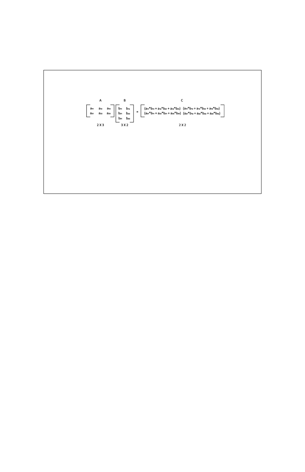
rows of one matrix with the columns of another matrix.

Below is an example:

Here we have the matrix A and the matrix B. A is a

2-by-3 matrix (2 rows and 3 columns), and B is a 3-by-2

matrix (3 rows

and 2 columns). The multiplication of AB is

compatible, which means

the number of columns of A is

equal to the number of rows in the second matrix, B. When

two compatible matrices are multiplied, their result has a

structure where the number of rows equals the number of

rows in the first matrix and the number of columns equals

the number of columns in the second matrix. The process

is the same for compatible matrices of any size.

Implementing

Matrix

Multiplication

Now let’s consider an algorithm for matrix multiplication.

To simplify things, let’s assume we have a Matrix class or

data structure that has a two-dimensional (2D) array.

Another way to think of a 2D array is as an array of

arrays. We could also think of this as a table with rows

and columns. The structure below gives a general example

of a Matrix class. Within this class, we also have

Figure 10.2

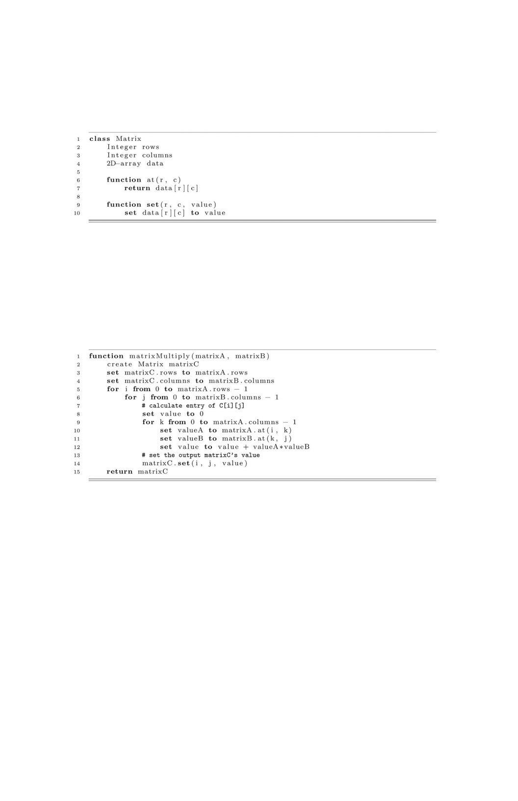
two convenience functions to access and set the values

of the matrix based on the row and column of the 2D

array.

With this structure for a Matrix class, we can

implement a matrix multiplication procedure. Below we

show the process of performing matrix multiplication on

two compatible matrices:

This function implements the matrix multiplication

procedure described above. On line 12, the new value of

the (i, j) entry in the result matrix is calculated. We see

that this involves a multiply operation and an addition

operation. On a typical processor, the multiply operation is

slower than addition. As we think about the complexity of

matrix multiplication, we will mainly consider the number

of multiplications. This is because as the matrices get

large, the cost associated with multiplication will dominate

the cost of addition. For this reason, we only consider the

number of multiplications.

So

how

many

multiplications

are

needed

for

matrix

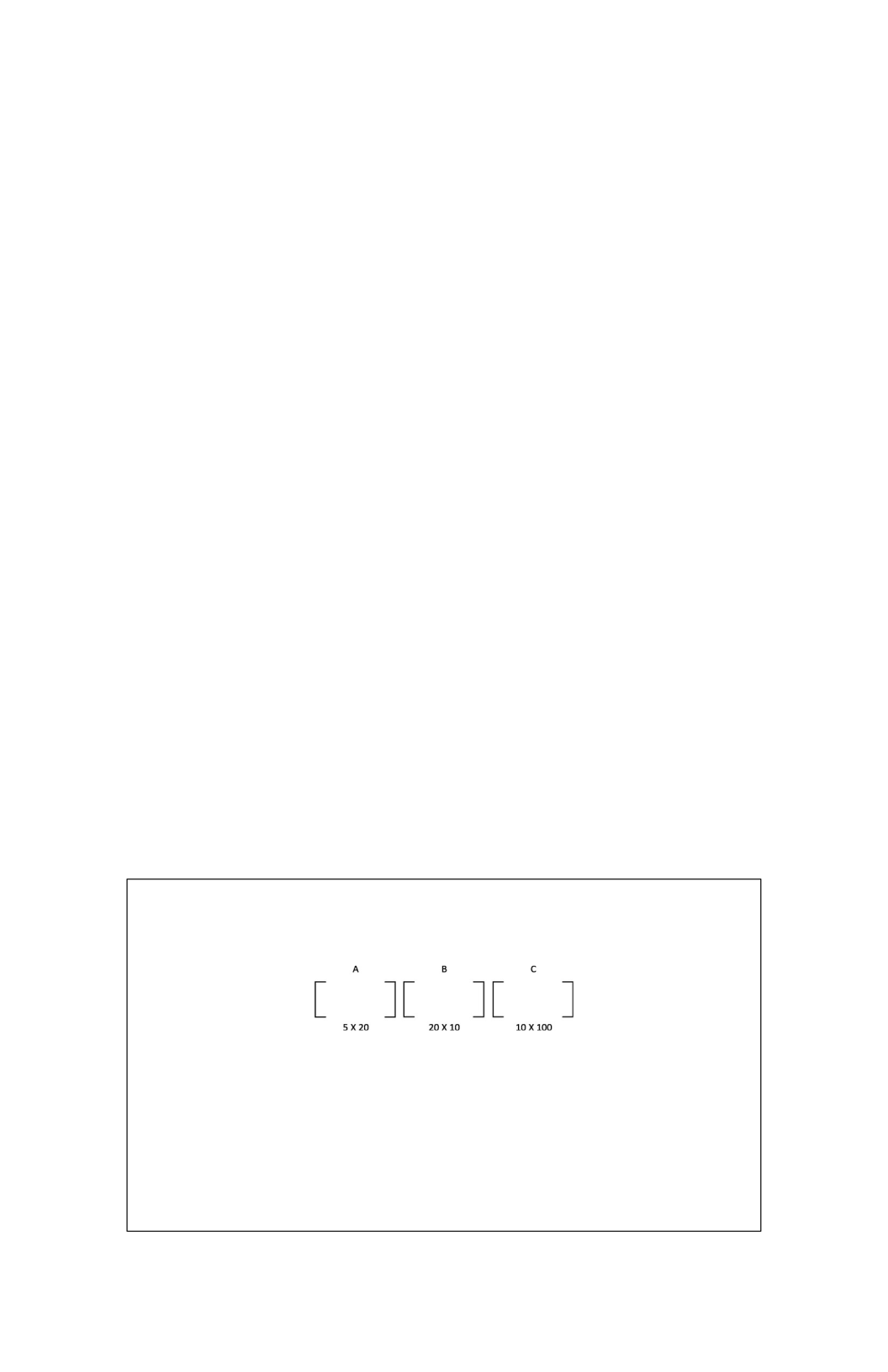
multiplication? The pattern above has a triple-nested loop.

This gives us a clue to the number of times the inner

code will run. As a result, we can expect the number of

multiplications to be equal to the number of times the

inner code will run. Let’s assume that matrix A has ra rows

and ca columns, and that matrix B, in a similar way, has rb

rows and cb columns. For A and B to be compatible

matrices, the value of ca would have to be equal to rb. We

know that the inner loop with index k runs a total of ca

times. This entire loop is executed once for every cb of B’s

columns (cb * ca). Finally, these two inner loops for j and k

would all run for every row in A, leading to multiplications

proportional to ra * ca * cb. This illustrates that as the size

of the matrices gets larger, the number of multiplications

grows quickly.

Why Order Matters

Now that we have seen how to multiply matrices together

and understand the computational cost, let’s consider just

why choosing to multiply in a specific order is important.

Suppose that we need to multiply three matrices—A, B,

and C—shown in the image below:

Figure 10.3

Multiplying them together could proceed with the

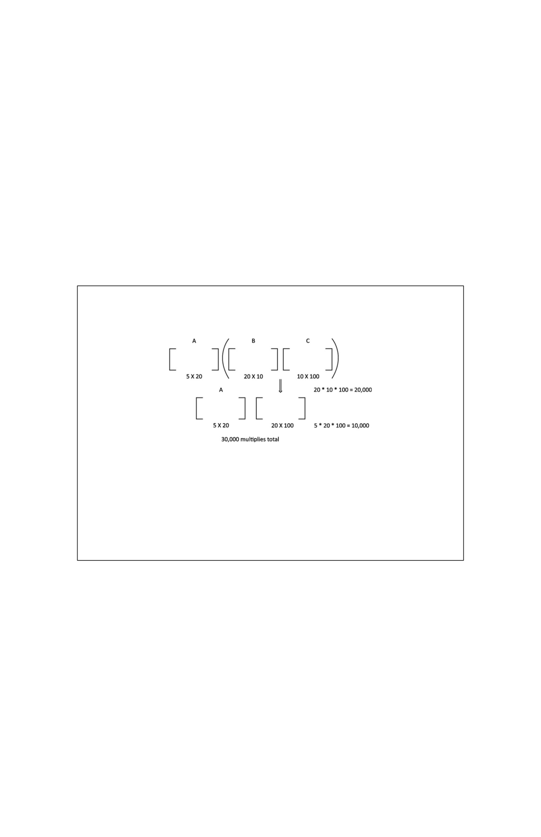
grouping (AB)C, where A and B are multiplied together

first, and then that result is multiplied by C. Alternatively, we

could group them as A(BC) and first multiply B by C, followed

by A multiplied by the result. Which would be better, or

would it even matter?

Let’s figure this out by first considering the A(BC)

grouping. The figure below illustrates this example. With

this grouping, calculating the BC multiplication yields

20,000 multiply operations. Multiplying A by this result

gives another 10,000 for a total of 30,000 multiply

operations.

Next, let’s consider the (AB)C grouping. The following

figure

shows a rough diagram of this calculation. The AB

matrix multiplication gives a cost of 1,000 multiply

operations. Then this result multiplied by C gives another

5,000. We now have a total of 6,000 multiply operations

for the (AB)C grouping over the other. This represents a

fivefold decrease in cost!

Figure 10.4

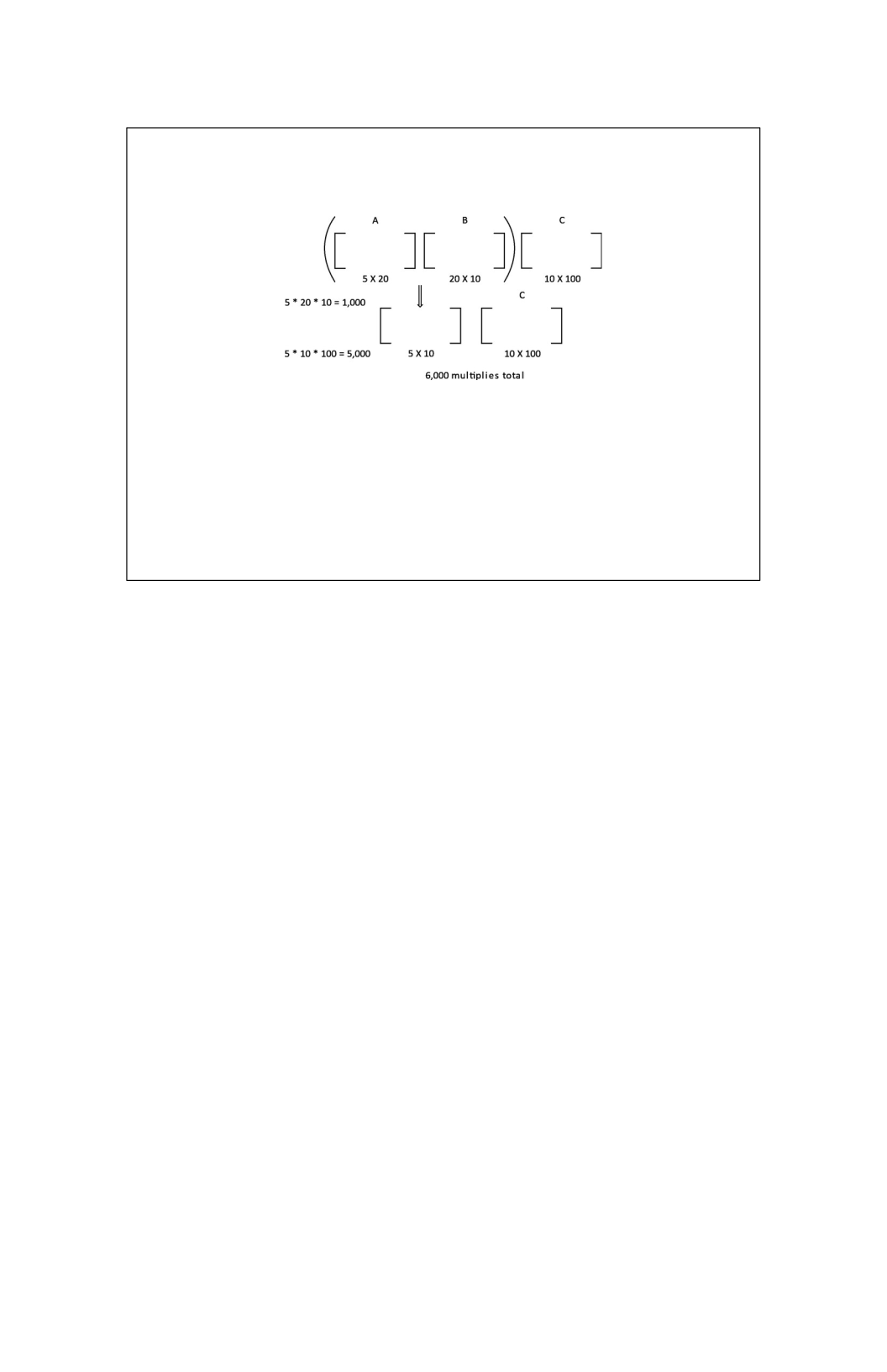
This example illustrates that the order of

multiplication definitely matters in terms of computational

cost. Additionally, as the matrices get larger, there could

be significant cost savings when we find an optimal

grouping for the multiplication sequence.

A Recursive Algorithm

for Optimal Matrix-Chain

Multiplication

We are interested in an algorithm for finding the optimal

ordering of matrix multiplication. This corresponds to

finding a grouping with a minimal cost. Suppose we have a

chain of 5 matrices, M

0

to M

4

. We could write their

dimensions as a list of 6 values. The 6 values come from

the fact that each sequential pair of matrices must be

compatible for multiplication to be possible. The figure

below shows this chain and gives the dimensions as a list.

Figure 10.5

An algorithm that minimizes the cost must find an

optimal split for the final two matrices. Let’s call these final

two matrices A and B. For the result to be optimal, then A

and B must both have resulted from an optimal subgrouping.

The possible splits would be

We need to evaluate these options by assessing

the cost of creating the A and B matrices (optimal

subproblems) as well as the cost of the final multiply, with

matrix A being multiplied by B. A recursive algorithm

would find the minimal cost by checking the minimum cost

among all splits. In the process of finding the cost of all

these four options for splits, we would need to calculate

the optimal splits for other sequences to find their optimal

groupings. This demonstrates the feature of optimal

substructure, the idea that an optimal solution could be

Figure 10.6

(M0) (M1 M2 M3 M4) = AB with a split after

position 0 (M0 M1) (M2 M3 M4) = AB with a split

after position 1 (M0 M1 M2) (M3 M4) = AB with a

split after position 2 (M0 M1 M2 M3) (M4) = AB

with a split after position 3.

built from optimal subproblems.

For the first grouping, we have A = M0 and B = (M1

M2 M3 M

4

). To calculate the cost of this split, it is

assumed that A and B have been constructed optimally.

This means that a recursive algorithm considering this split

must then make a recursive call to

find the minimal

grouping for (M1 M2 M3 M4) for the B matrix. This in

turn

would trigger another search for the optimal split among

(M

1

) (M2 M3 M4) (M1 M2) (M3 M4) and (M1 M2 M3) (M4). We

can also see

that this would trigger further calls to optimize each

sequence of 3 matrices and so on. You may be able to

imagine that this recursive process has a high branch

factor leading to an exponential runtime complexity in the

number of matrices. With n matrices, the runtime

complexity would be even worse than O(2n), exponential time. It

would follow an algorithm for calculating the Catalan

numbers at O(3n).

A general outline of the recursive algorithm would be

as follows. We will consider an algorithm to calculate the

minimal cost of multiplying a sequence of matrices starting at

some matrix identified by the start index and including the

ending matrix using an end index. The base case of the

algorithm is when start and end are equal. The cost of

multiplication of only one matrix is 0 as there is no

operation to perform. The recursive case calculates the cost

of splitting the sequence at some split position. There will be

n − 1 split positions to test when considering n matrices

where n = end − start

+ 1, and the recursive algorithm will need to find the

minimum of the options for the best split position.

To complete the recursive algorithm, we will

introduce a function to calculate the cost of the final

multiplication. This could be a simple multiplication of the

correct dimensions, but we will introduce and explain this

function to make the meaning clear and to simplify some

of the code (which would otherwise include a lot of

awkward indexing). The figure below illustrates what is

meant by the final multiplication:

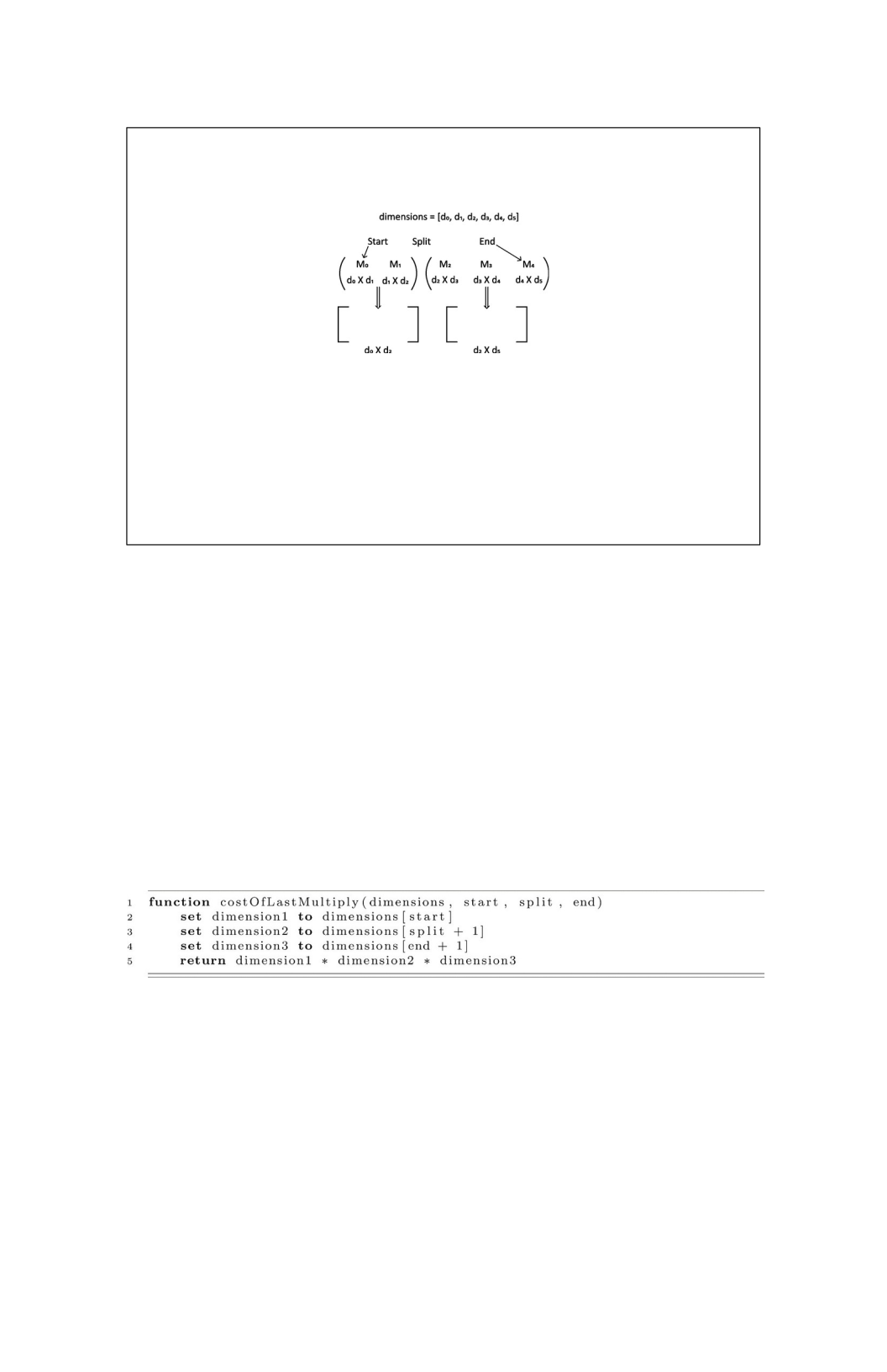
Suppose we are calculating the number of

multiplications for a split at index 1 (or just after M1). The

algorithm would have given the optimal cost for constructing

the left matrix and the right matrix, but we would still need to

calculate the cost of multiplying those together. The left

matrix would have dimensions of d0 by d2 and the right

matrix would have dimensions of d2 by d5. Using the

dimensions list and indexes for start, split, and end, we can

calculate this cost. The function below performs this operation

in a way that might make the meaning a little clearer. Notice

that for matrix i, the dimensions of that matrix are di by di+1.

With this helper function, we can now write the

recursive algorithm.

Figure 10.7

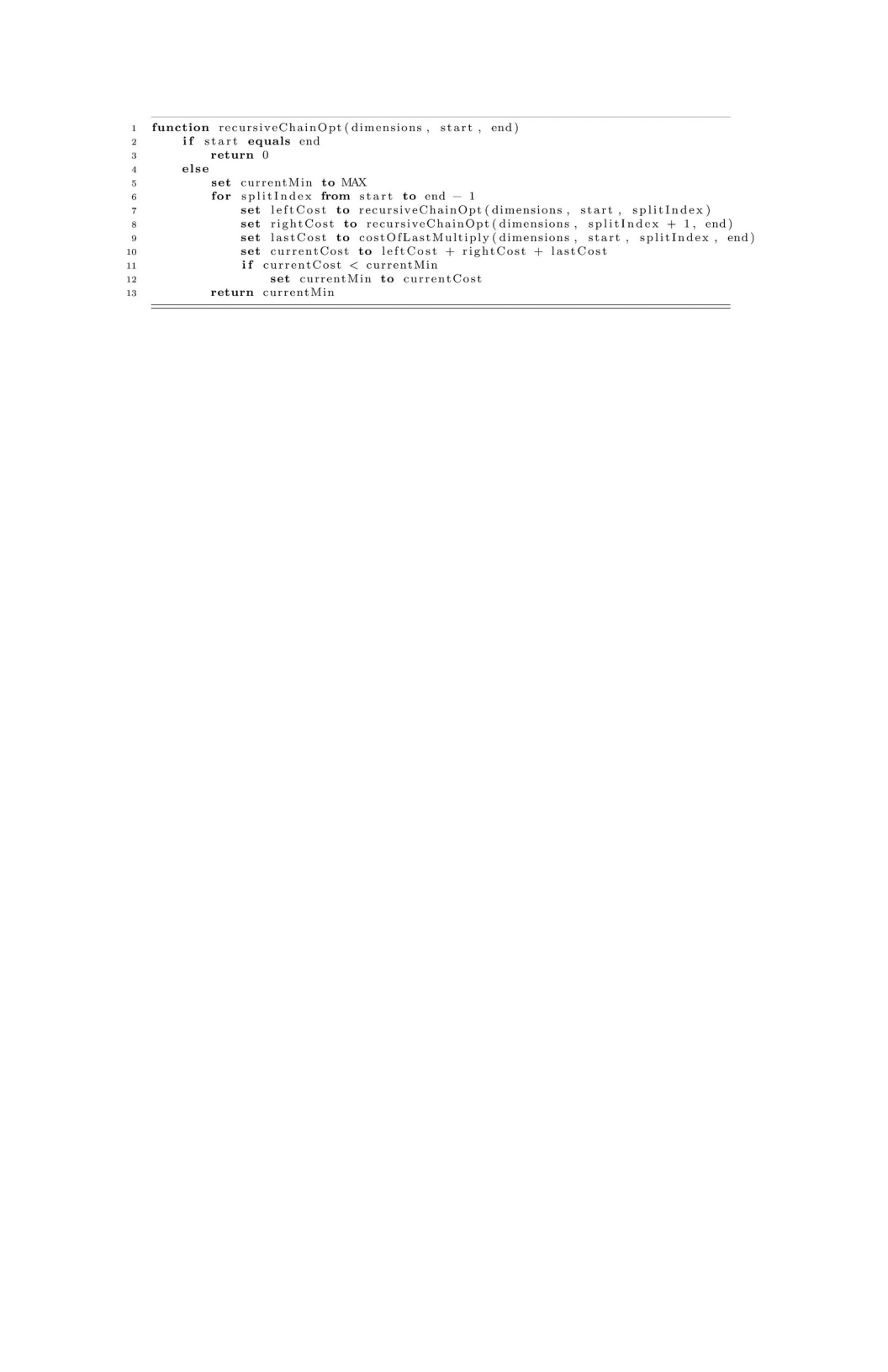
This algorithm only calculates an optimal cost, but

it could be modified to record the split indexes of the

optimal splits so that another process could use that

information. The optimal cost of multiplying all matrices in

the optimal grouping could be calculated with a call to

recursiveChainOpt(dimensions, 0, 4). This algorithm, while

correct, suffers from exponential time complexity. This is

the type of situation where dynamic programming can

help.

Requirements for Applying

Dynamic Programming

There are two main requirements for applying dynamic

programming. First, a problem must exhibit the property

known as optimal substructure. This means that an

optimal solution to the problem is constructed from

optimal solutions to the subproblems. We will see an

example of this soon. The second property is called

overlapping subproblems. This means that subproblems

are shared. We saw this in our Fibonacci example.

Optimal Matrix Chain Multiplication

A classic application of dynamic programming concerns

the optimal multiplication order for matrices. Consider the

sequence of matrices {M1, M2, M3, M4}. There are several

ways to multiply these together. These ways correspond

to the number of distinct ways to parenthesize the matrix

multiplication order. For the mathematically curious, the

Catalan numbers give the total number of possible ways.

For example, one way to group these would be (M

1

M2) (M3

M4). Another way could be M1 ((M2 M3) M4). Any grouping

leads to the same final result, but the number of multiply

operations of the overall calculation could differ greatly

with different groupings. To understand this idea, let’s

review matrix multiplication.

Matrix

Multiplication

Review

Matrix multiplication is an operation that multiplies and adds the

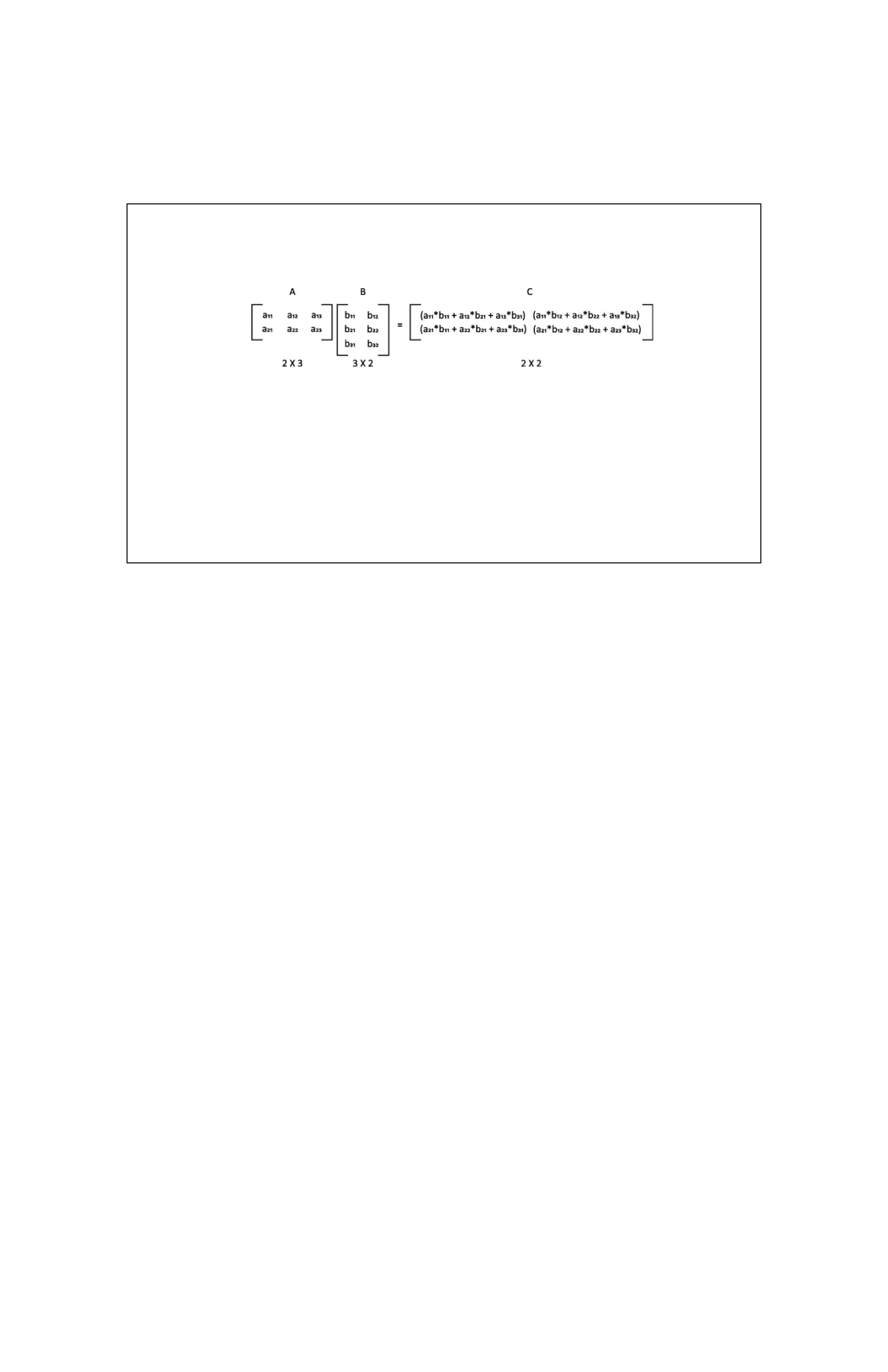
rows of one matrix with the columns of another matrix.

Below is an example:

Here we have the matrix A and the matrix B. A is a

2-by-3 matrix (2 rows and 3 columns), and B is a 3-by-2

matrix (3 rows

and 2 columns). The multiplication of AB is

compatible, which means

the number of columns of A is

equal to the number of rows in the second matrix, B. When

two compatible matrices are multiplied, their result has a

structure where the number of rows equals the number of

rows in the first matrix and the number of columns equals

the number of columns in the second matrix. The process

is the same for compatible matrices of any size.

Implementing

Matrix

Multiplication

Now let’s consider an algorithm for matrix multiplication.

To simplify things, let’s assume we have a Matrix class or

data structure that has a two-dimensional (2D) array.

Another way to think of a 2D array is as an array of

arrays. We could also think of this as a table with rows

and columns. The structure below gives a general example

of a Matrix class. Within this class, we also have

Figure 10.2

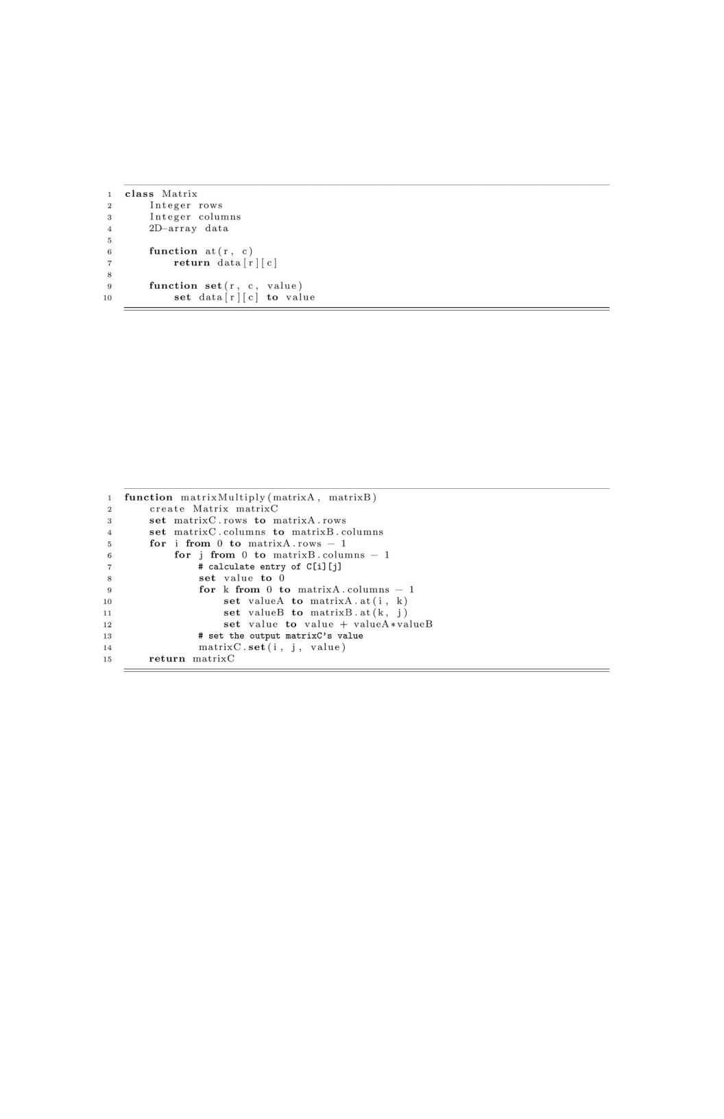
two convenience functions to access and set the values

of the matrix based on the row and column of the 2D

array.

With this structure for a Matrix class, we can

implement a matrix multiplication procedure. Below we

show the process of performing matrix multiplication on

two compatible matrices:

This function implements the matrix multiplication

procedure described above. On line 12, the new value of

the (i, j) entry in the result matrix is calculated. We see

that this involves a multiply operation and an addition

operation. On a typical processor, the multiply operation is

slower than addition. As we think about the complexity of

matrix multiplication, we will mainly consider the number

of multiplications. This is because as the matrices get

large, the cost associated with multiplication will dominate

the cost of addition. For this reason, we only consider the

number of multiplications.

So

how

many

multiplications

are

needed

for

matrix

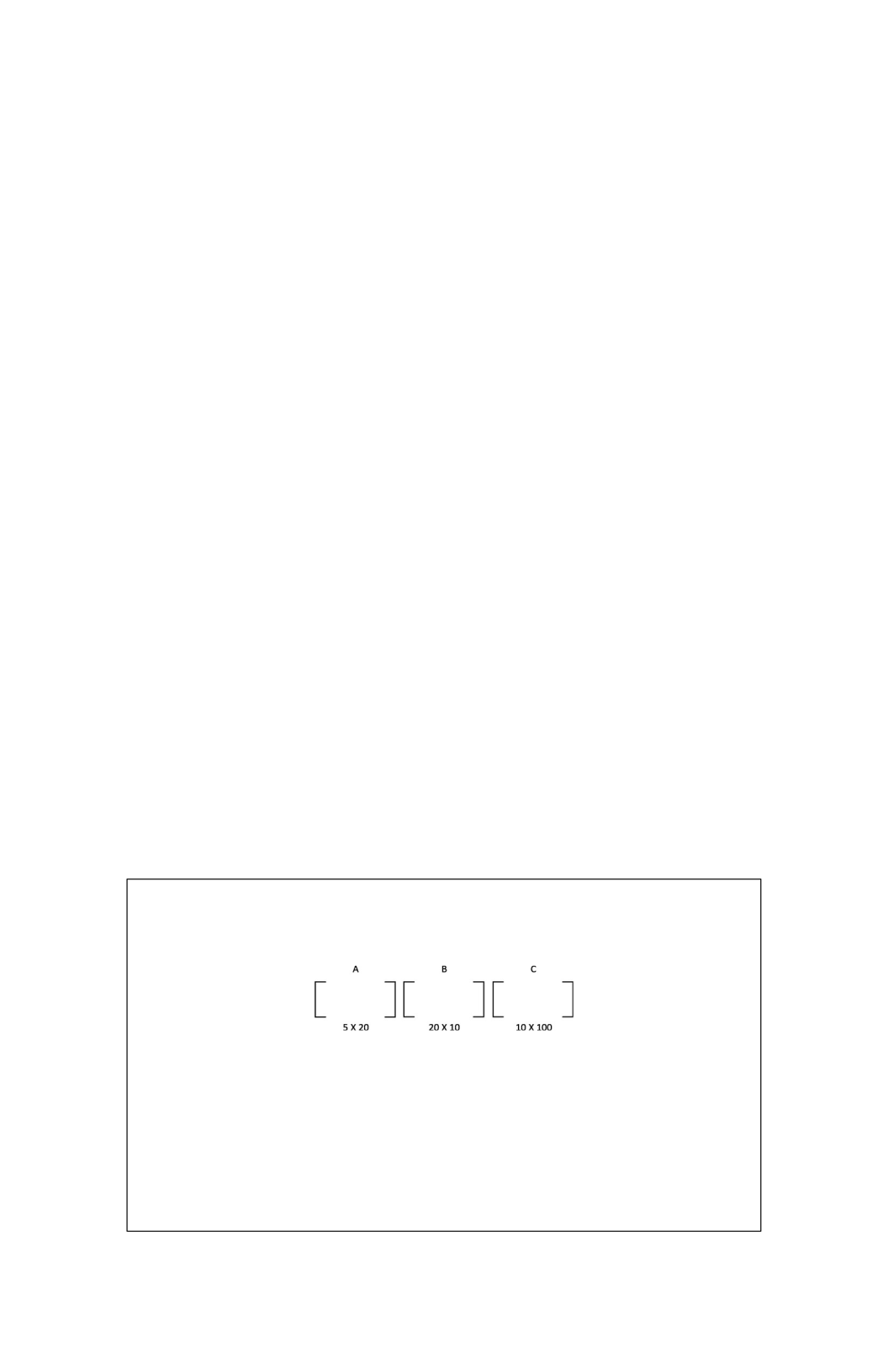
multiplication? The pattern above has a triple-nested loop.

This gives us a clue to the number of times the inner

code will run. As a result, we can expect the number of

multiplications to be equal to the number of times the

inner code will run. Let’s assume that matrix A has ra rows

and ca columns, and that matrix B, in a similar way, has rb

rows and cb columns. For A and B to be compatible

matrices, the value of ca would have to be equal to rb. We

know that the inner loop with index k runs a total of ca

times. This entire loop is executed once for every cb of B’s

columns (cb * ca). Finally, these two inner loops for j and k

would all run for every row in A, leading to multiplications

proportional to ra * ca * cb. This illustrates that as the size

of the matrices gets larger, the number of multiplications

grows quickly.

Why Order Matters

Now that we have seen how to multiply matrices together

and understand the computational cost, let’s consider just

why choosing to multiply in a specific order is important.

Suppose that we need to multiply three matrices—A, B,

and C—shown in the image below:

Figure 10.3

Multiplying them together could proceed with the

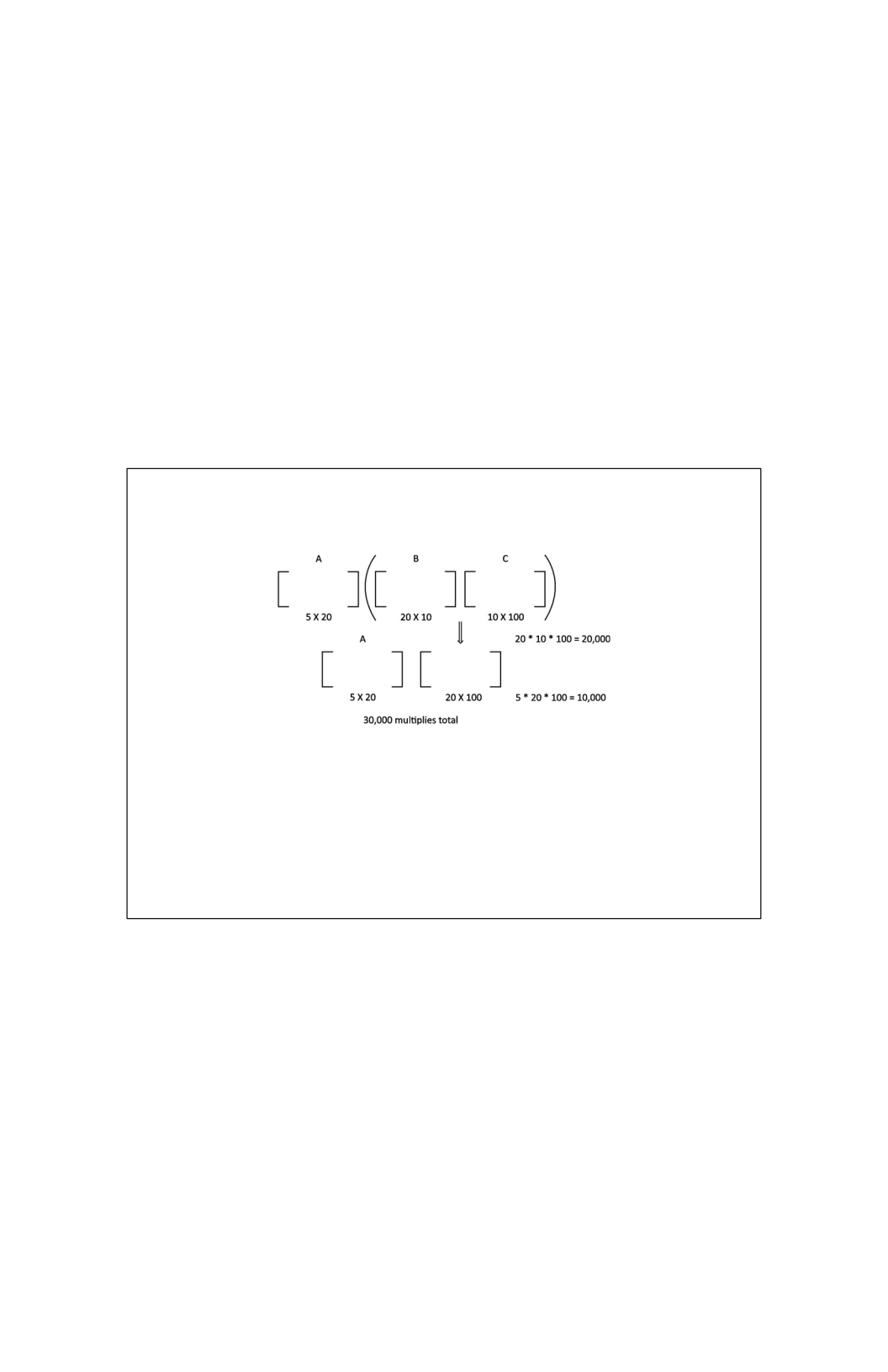
grouping (AB)C, where A and B are multiplied together

first, and then that result is multiplied by C. Alternatively, we

could group them as A(BC) and first multiply B by C, followed

by A multiplied by the result. Which would be better, or

would it even matter?

Let’s figure this out by first considering the A(BC)

grouping. The figure below illustrates this example. With

this grouping, calculating the BC multiplication yields

20,000 multiply operations. Multiplying A by this result

gives another 10,000 for a total of 30,000 multiply

operations.

Next, let’s consider the (AB)C grouping. The following

figure

shows a rough diagram of this calculation. The AB

matrix multiplication gives a cost of 1,000 multiply

operations. Then this result multiplied by C gives another

5,000. We now have a total of 6,000 multiply operations

for the (AB)C grouping over the other. This represents a

fivefold decrease in cost!

Figure 10.4

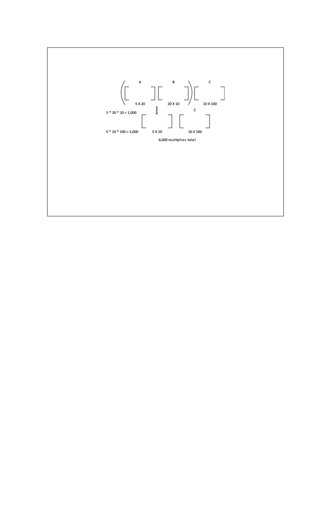
This example illustrates that the order of

multiplication definitely matters in terms of computational

cost. Additionally, as the matrices get larger, there could

be significant cost savings when we find an optimal

grouping for the multiplication sequence.

A Recursive Algorithm

for Optimal Matrix-Chain

Multiplication

We are interested in an algorithm for finding the optimal

ordering of matrix multiplication. This corresponds to

finding a grouping with a minimal cost. Suppose we have a

chain of 5 matrices, M

0

to M

4

. We could write their

dimensions as a list of 6 values. The 6 values come from

the fact that each sequential pair of matrices must be

compatible for multiplication to be possible. The figure

below shows this chain and gives the dimensions as a list.

Figure 10.5

An algorithm that minimizes the cost must find an

optimal split for the final two matrices. Let’s call these final

two matrices A and B. For the result to be optimal, then A

and B must both have resulted from an optimal subgrouping.

The possible splits would be

We need to evaluate these options by assessing

the cost of creating the A and B matrices (optimal

subproblems) as well as the cost of the final multiply, with

matrix A being multiplied by B. A recursive algorithm

would find the minimal cost by checking the minimum cost

among all splits. In the process of finding the cost of all

these four options for splits, we would need to calculate

the optimal splits for other sequences to find their optimal

groupings. This demonstrates the feature of optimal

substructure, the idea that an optimal solution could be

Figure 10.6

(M0) (M1 M2 M3 M4) = AB with a split after

position 0 (M0 M1) (M2 M3 M4) = AB with a split

after position 1 (M0 M1 M2) (M3 M4) = AB with a

split after position 2 (M0 M1 M2 M3) (M4) = AB

with a split after position 3.

built from optimal subproblems.

For the first grouping, we have A = M0 and B = (M1

M2 M3 M

4

). To calculate the cost of this split, it is

assumed that A and B have been constructed optimally.

This means that a recursive algorithm considering this split

must then make a recursive call to

find the minimal

grouping for (M1 M2 M3 M4) for the B matrix. This in

turn

would trigger another search for the optimal split among

(M

1

) (M2 M3 M4) (M1 M2) (M3 M4) and (M1 M2 M3) (M4). We

can also see

that this would trigger further calls to optimize each

sequence of 3 matrices and so on. You may be able to

imagine that this recursive process has a high branch

factor leading to an exponential runtime complexity in the

number of matrices. With n matrices, the runtime

complexity would be even worse than O(2n), exponential time. It

would follow an algorithm for calculating the Catalan

numbers at O(3n).

A general outline of the recursive algorithm would be

as follows. We will consider an algorithm to calculate the

minimal cost of multiplying a sequence of matrices starting at

some matrix identified by the start index and including the

ending matrix using an end index. The base case of the

algorithm is when start and end are equal. The cost of

multiplication of only one matrix is 0 as there is no

operation to perform. The recursive case calculates the cost

of splitting the sequence at some split position. There will be

n − 1 split positions to test when considering n matrices

where n = end − start

+ 1, and the recursive algorithm will need to find the

minimum of the options for the best split position.

To complete the recursive algorithm, we will

introduce a function to calculate the cost of the final

multiplication. This could be a simple multiplication of the

correct dimensions, but we will introduce and explain this

function to make the meaning clear and to simplify some

of the code (which would otherwise include a lot of

awkward indexing). The figure below illustrates what is

meant by the final multiplication:

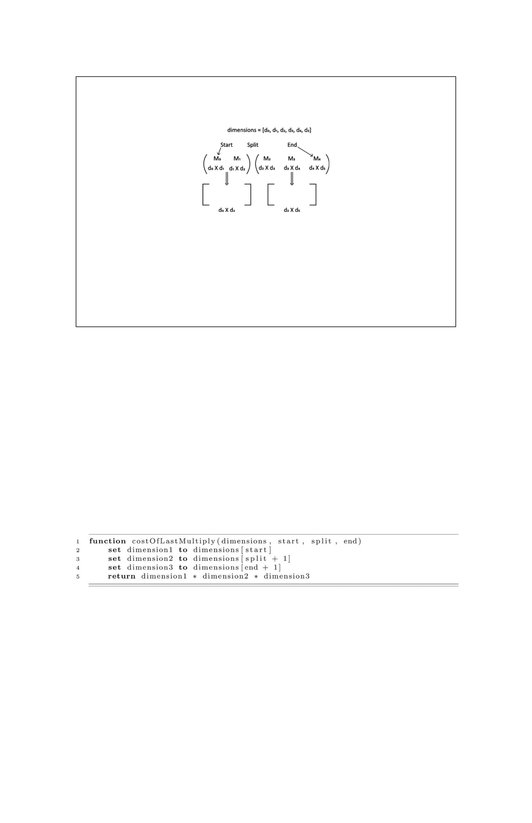
Suppose we are calculating the number of

multiplications for a split at index 1 (or just after M1). The

algorithm would have given the optimal cost for constructing

the left matrix and the right matrix, but we would still need to

calculate the cost of multiplying those together. The left

matrix would have dimensions of d0 by d2 and the right

matrix would have dimensions of d2 by d5. Using the

dimensions list and indexes for start, split, and end, we can

calculate this cost. The function below performs this operation

in a way that might make the meaning a little clearer. Notice

that for matrix i, the dimensions of that matrix are di by di+1.

With this helper function, we can now write the

recursive algorithm.

Figure 10.7

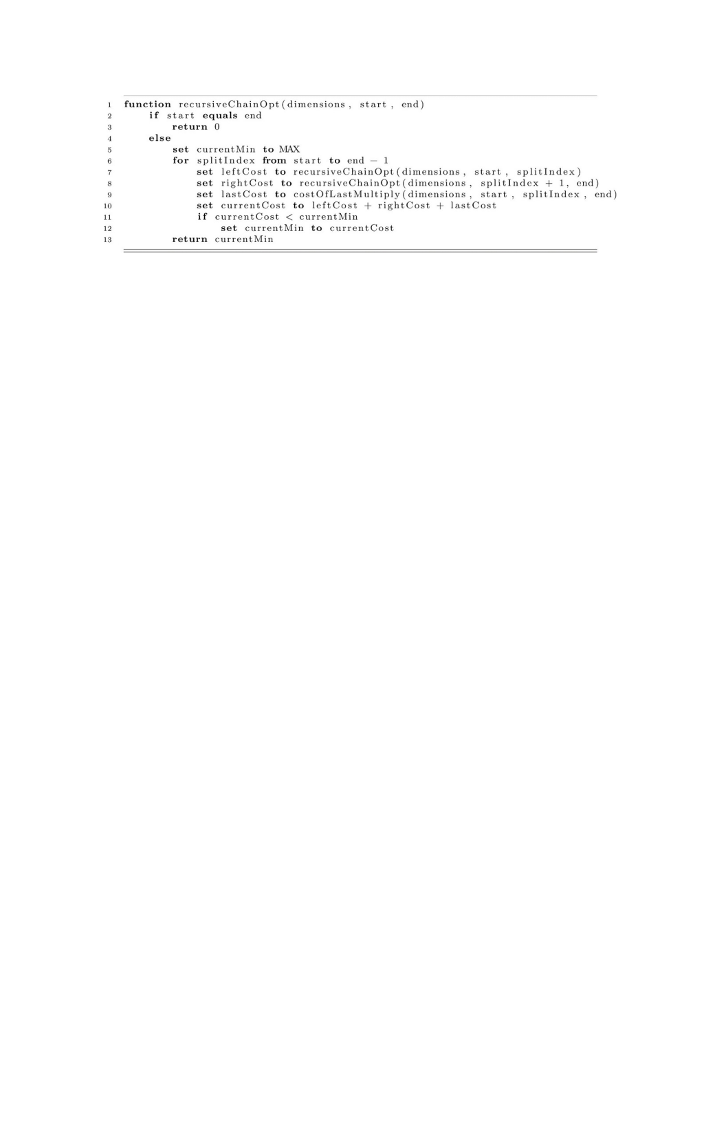
This algorithm only calculates an optimal cost, but

it could be modified to record the split indexes of the

optimal splits so that another process could use that

information. The optimal cost of multiplying all matrices in

the optimal grouping could be calculated with a call to

recursiveChainOpt(dimensions, 0, 4). This algorithm, while

correct, suffers from exponential time complexity. This is

the type of situation where dynamic programming can

help.

Requirements for Applying

Dynamic Programming

There are two main requirements for applying dynamic

programming. First, a problem must exhibit the property

known as optimal substructure. This means that an

optimal solution to the problem is constructed from

optimal solutions to the subproblems. We will see an

example of this soon. The second property is called

overlapping subproblems. This means that subproblems

are shared. We saw this in our Fibonacci example.

Optimal Matrix Chain Multiplication

A classic application of dynamic programming concerns

the optimal multiplication order for matrices. Consider the

sequence of matrices {M1, M2, M3, M4}. There are several

ways to multiply these together. These ways correspond

to the number of distinct ways to parenthesize the matrix

multiplication order. For the mathematically curious, the

Catalan numbers give the total number of possible ways.

For example, one way to group these would be (M

1

M2) (M3

M4). Another way could be M1 ((M2 M3) M4). Any grouping

leads to the same final result, but the number of multiply

operations of the overall calculation could differ greatly

with different groupings. To understand this idea, let’s

review matrix multiplication.

Matrix

Multiplication

Review

Matrix multiplication is an operation that multiplies and adds the

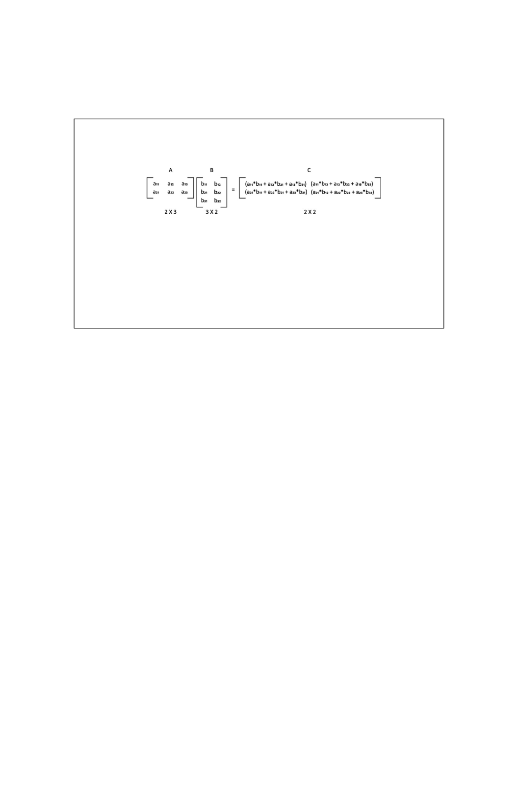
rows of one matrix with the columns of another matrix.

Below is an example:

Here we have the matrix A and the matrix B. A is a

2-by-3 matrix (2 rows and 3 columns), and B is a 3-by-2

matrix (3 rows

and 2 columns). The multiplication of AB is

compatible, which means

the number of columns of A is

equal to the number of rows in the second matrix, B. When

two compatible matrices are multiplied, their result has a

structure where the number of rows equals the number of

rows in the first matrix and the number of columns equals

the number of columns in the second matrix. The process

is the same for compatible matrices of any size.

Implementing

Matrix

Multiplication

Now let’s consider an algorithm for matrix multiplication.

To simplify things, let’s assume we have a Matrix class or

data structure that has a two-dimensional (2D) array.

Another way to think of a 2D array is as an array of

arrays. We could also think of this as a table with rows

and columns. The structure below gives a general example

of a Matrix class. Within this class, we also have

Figure 10.2

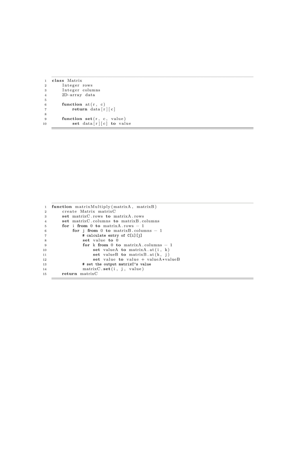
two convenience functions to access and set the values

of the matrix based on the row and column of the 2D

array.

With this structure for a Matrix class, we can

implement a matrix multiplication procedure. Below we

show the process of performing matrix multiplication on

two compatible matrices:

This function implements the matrix multiplication

procedure described above. On line 12, the new value of

the (i, j) entry in the result matrix is calculated. We see

that this involves a multiply operation and an addition

operation. On a typical processor, the multiply operation is

slower than addition. As we think about the complexity of

matrix multiplication, we will mainly consider the number

of multiplications. This is because as the matrices get

large, the cost associated with multiplication will dominate

the cost of addition. For this reason, we only consider the

number of multiplications.

So

how

many

multiplications

are

needed

for

matrix

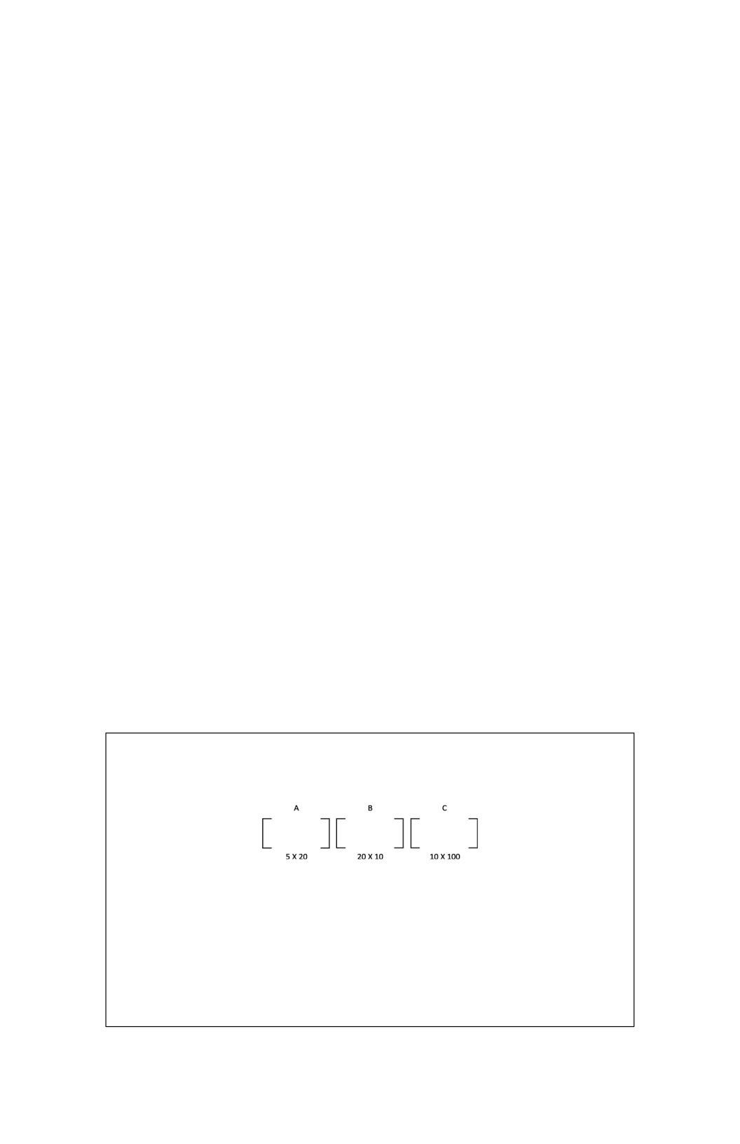
multiplication? The pattern above has a triple-nested loop.

This gives us a clue to the number of times the inner

code will run. As a result, we can expect the number of

multiplications to be equal to the number of times the

inner code will run. Let’s assume that matrix A has ra rows

and ca columns, and that matrix B, in a similar way, has rb

rows and cb columns. For A and B to be compatible

matrices, the value of ca would have to be equal to rb. We

know that the inner loop with index k runs a total of ca

times. This entire loop is executed once for every cb of B’s

columns (cb * ca). Finally, these two inner loops for j and k

would all run for every row in A, leading to multiplications

proportional to ra * ca * cb. This illustrates that as the size

of the matrices gets larger, the number of multiplications

grows quickly.

Why Order Matters

Now that we have seen how to multiply matrices together

and understand the computational cost, let’s consider just

why choosing to multiply in a specific order is important.

Suppose that we need to multiply three matrices—A, B,

and C—shown in the image below:

Figure 10.3

Multiplying them together could proceed with the

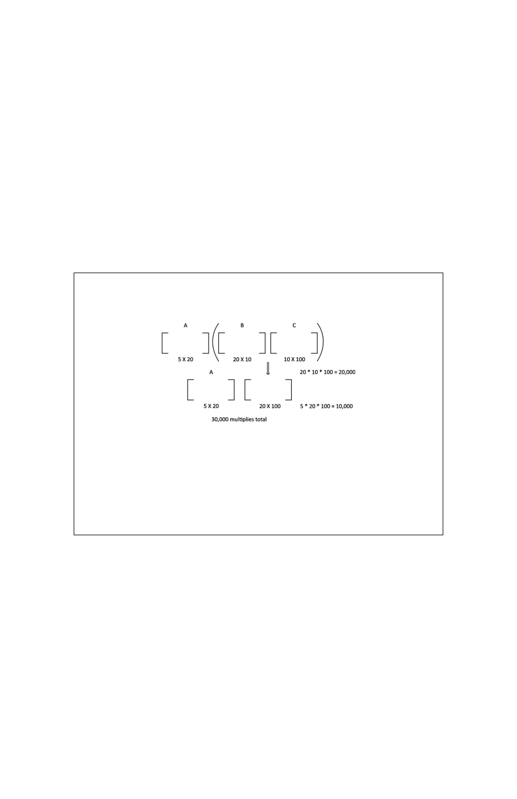
grouping (AB)C, where A and B are multiplied together

first, and then that result is multiplied by C. Alternatively, we

could group them as A(BC) and first multiply B by C, followed

by A multiplied by the result. Which would be better, or

would it even matter?

Let’s figure this out by first considering the A(BC)

grouping. The figure below illustrates this example. With

this grouping, calculating the BC multiplication yields

20,000 multiply operations. Multiplying A by this result

gives another 10,000 for a total of 30,000 multiply

operations.

Next, let’s consider the (AB)C grouping. The following

figure

shows a rough diagram of this calculation. The AB

matrix multiplication gives a cost of 1,000 multiply

operations. Then this result multiplied by C gives another

5,000. We now have a total of 6,000 multiply operations

for the (AB)C grouping over the other. This represents a

fivefold decrease in cost!

Figure 10.4

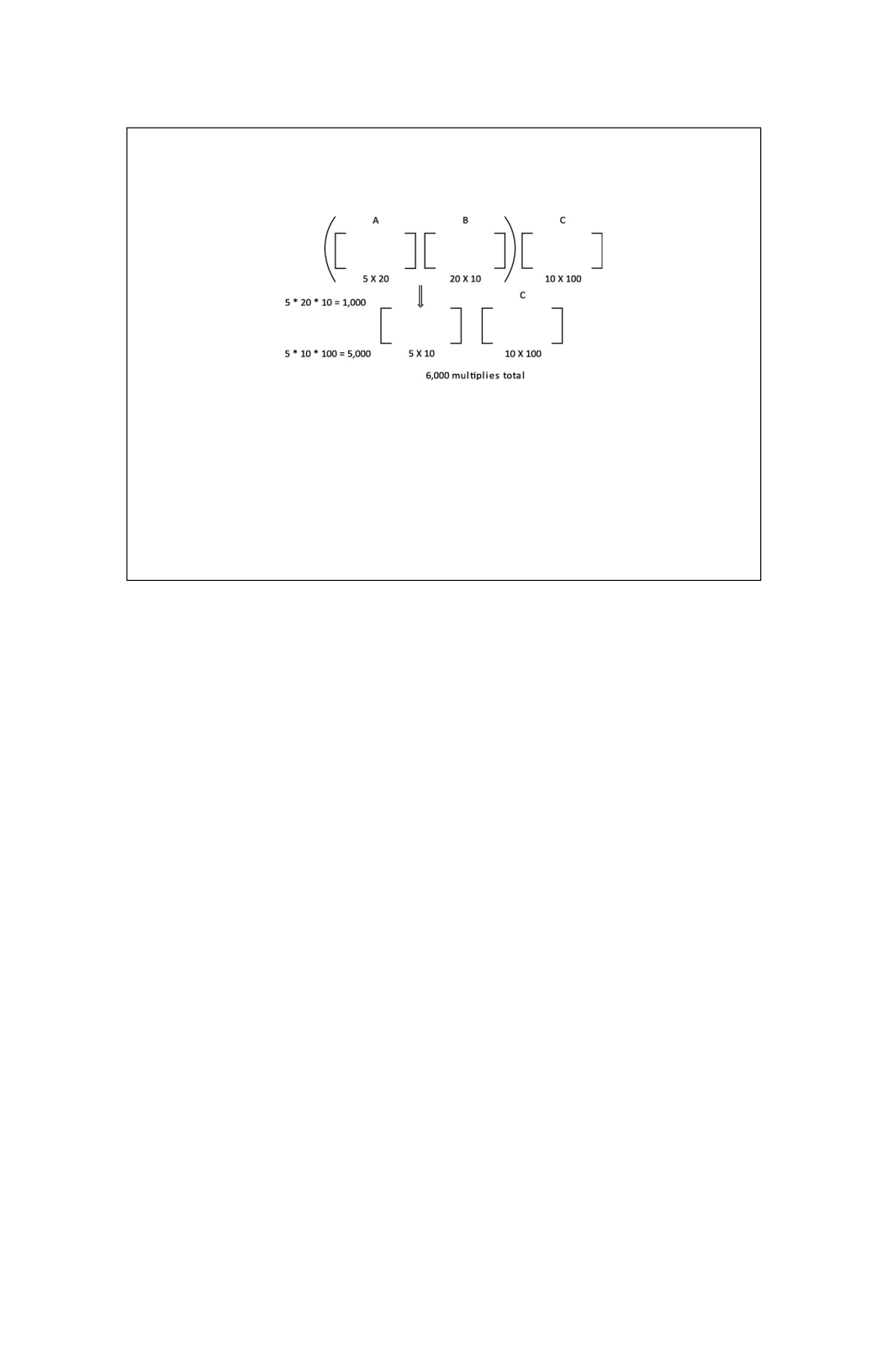
This example illustrates that the order of

multiplication definitely matters in terms of computational

cost. Additionally, as the matrices get larger, there could

be significant cost savings when we find an optimal

grouping for the multiplication sequence.

A Recursive Algorithm

for Optimal Matrix-Chain

Multiplication

We are interested in an algorithm for finding the optimal

ordering of matrix multiplication. This corresponds to

finding a grouping with a minimal cost. Suppose we have a

chain of 5 matrices, M

0

to M

4

. We could write their

dimensions as a list of 6 values. The 6 values come from

the fact that each sequential pair of matrices must be

compatible for multiplication to be possible. The figure

below shows this chain and gives the dimensions as a list.

Figure 10.5

An algorithm that minimizes the cost must find an

optimal split for the final two matrices. Let’s call these final

two matrices A and B. For the result to be optimal, then A

and B must both have resulted from an optimal subgrouping.

The possible splits would be

We need to evaluate these options by assessing

the cost of creating the A and B matrices (optimal

subproblems) as well as the cost of the final multiply, with

matrix A being multiplied by B. A recursive algorithm

would find the minimal cost by checking the minimum cost

among all splits. In the process of finding the cost of all

these four options for splits, we would need to calculate

the optimal splits for other sequences to find their optimal

groupings. This demonstrates the feature of optimal

substructure, the idea that an optimal solution could be

Figure 10.6

(M0) (M1 M2 M3 M4) = AB with a split after

position 0 (M0 M1) (M2 M3 M4) = AB with a split

after position 1 (M0 M1 M2) (M3 M4) = AB with a

split after position 2 (M0 M1 M2 M3) (M4) = AB

with a split after position 3.

built from optimal subproblems.

For the first grouping, we have A = M0 and B = (M1

M2 M3 M

4

). To calculate the cost of this split, it is

assumed that A and B have been constructed optimally.

This means that a recursive algorithm considering this split

must then make a recursive call to

find the minimal

grouping for (M1 M2 M3 M4) for the B matrix. This in

turn

would trigger another search for the optimal split among

(M

1

) (M2 M3 M4) (M1 M2) (M3 M4) and (M1 M2 M3) (M4). We

can also see

that this would trigger further calls to optimize each

sequence of 3 matrices and so on. You may be able to

imagine that this recursive process has a high branch

factor leading to an exponential runtime complexity in the

number of matrices. With n matrices, the runtime

complexity would be even worse than O(2n), exponential time. It

would follow an algorithm for calculating the Catalan

numbers at O(3n).

A general outline of the recursive algorithm would be

as follows. We will consider an algorithm to calculate the

minimal cost of multiplying a sequence of matrices starting at

some matrix identified by the start index and including the

ending matrix using an end index. The base case of the

algorithm is when start and end are equal. The cost of

multiplication of only one matrix is 0 as there is no

operation to perform. The recursive case calculates the cost

of splitting the sequence at some split position. There will be

n − 1 split positions to test when considering n matrices

where n = end − start

+ 1, and the recursive algorithm will need to find the

minimum of the options for the best split position.

To complete the recursive algorithm, we will

introduce a function to calculate the cost of the final

multiplication. This could be a simple multiplication of the

correct dimensions, but we will introduce and explain this

function to make the meaning clear and to simplify some

of the code (which would otherwise include a lot of

awkward indexing). The figure below illustrates what is

meant by the final multiplication:

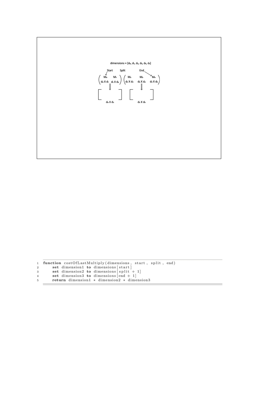
Suppose we are calculating the number of

multiplications for a split at index 1 (or just after M1). The

algorithm would have given the optimal cost for constructing

the left matrix and the right matrix, but we would still need to

calculate the cost of multiplying those together. The left

matrix would have dimensions of d0 by d2 and the right

matrix would have dimensions of d2 by d5. Using the

dimensions list and indexes for start, split, and end, we can

calculate this cost. The function below performs this operation

in a way that might make the meaning a little clearer. Notice

that for matrix i, the dimensions of that matrix are di by di+1.

With this helper function, we can now write the

recursive algorithm.

Figure 10.7

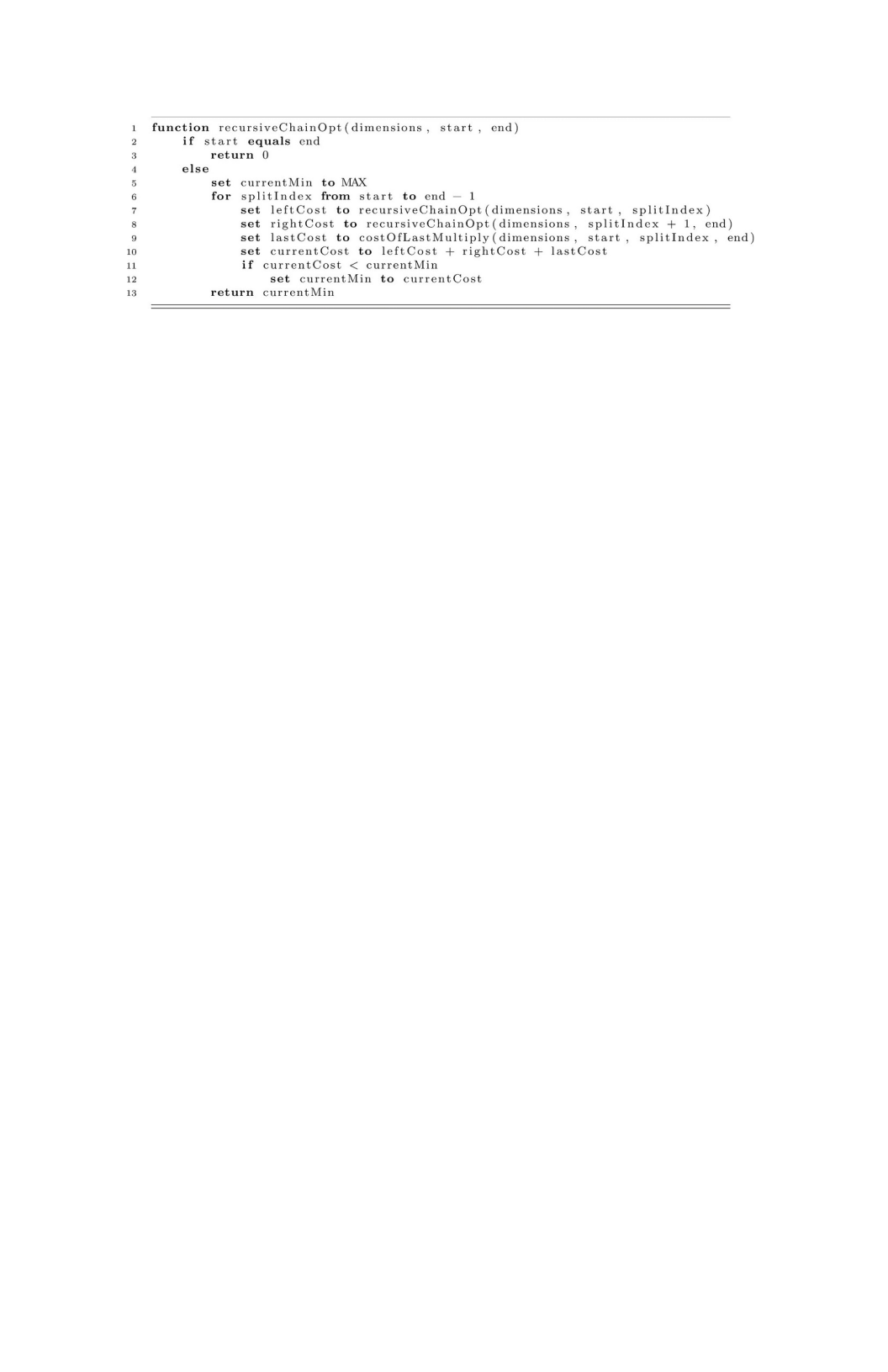
This algorithm only calculates an optimal cost, but

it could be modified to record the split indexes of the

optimal splits so that another process could use that

information. The optimal cost of multiplying all matrices in

the optimal grouping could be calculated with a call to

recursiveChainOpt(dimensions, 0, 4). This algorithm, while

correct, suffers from exponential time complexity. This is

the type of situation where dynamic programming can

help.

Requirements for Applying

Dynamic Programming

There are two main requirements for applying dynamic

programming. First, a problem must exhibit the property

known as optimal substructure. This means that an

optimal solution to the problem is constructed from

optimal solutions to the subproblems. We will see an

example of this soon. The second property is called

overlapping subproblems. This means that subproblems

are shared. We saw this in our Fibonacci example.

Optimal Matrix Chain Multiplication

A classic application of dynamic programming concerns

the optimal multiplication order for matrices. Consider the

sequence of matrices {M1, M2, M3, M4}. There are several

ways to multiply these together. These ways correspond

to the number of distinct ways to parenthesize the matrix

multiplication order. For the mathematically curious, the

Catalan numbers give the total number of possible ways.

For example, one way to group these would be (M

1

M2) (M3

M4). Another way could be M1 ((M2 M3) M4). Any grouping

leads to the same final result, but the number of multiply

operations of the overall calculation could differ greatly

with different groupings. To understand this idea, let’s

review matrix multiplication.

Matrix

Multiplication

Review

Matrix multiplication is an operation that multiplies and adds the

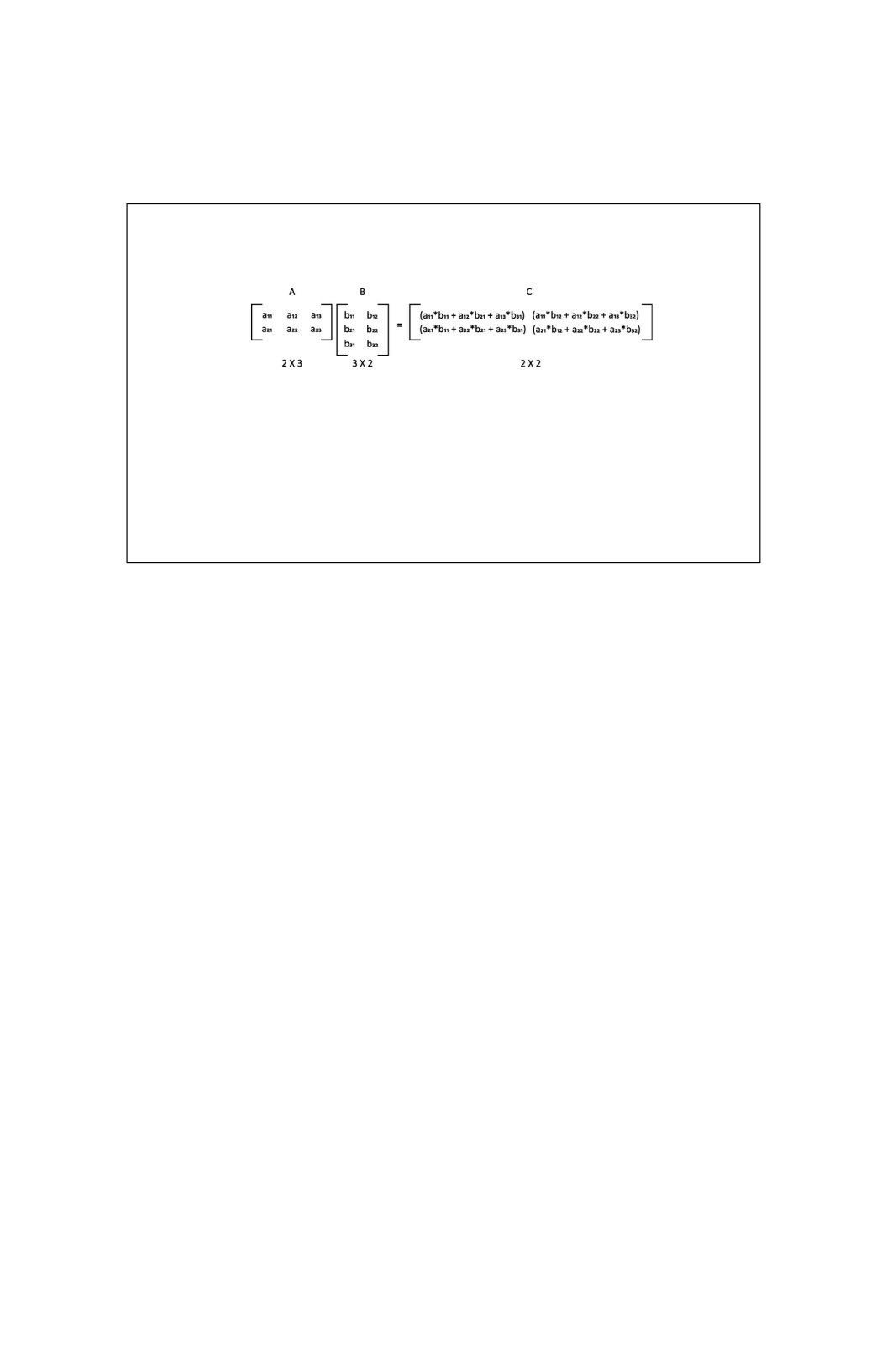
rows of one matrix with the columns of another matrix.

Below is an example:

Here we have the matrix A and the matrix B. A is a

2-by-3 matrix (2 rows and 3 columns), and B is a 3-by-2

matrix (3 rows

and 2 columns). The multiplication of AB is

compatible, which means

the number of columns of A is

equal to the number of rows in the second matrix, B. When

two compatible matrices are multiplied, their result has a

structure where the number of rows equals the number of

rows in the first matrix and the number of columns equals

the number of columns in the second matrix. The process

is the same for compatible matrices of any size.

Implementing

Matrix

Multiplication

Now let’s consider an algorithm for matrix multiplication.

To simplify things, let’s assume we have a Matrix class or

data structure that has a two-dimensional (2D) array.

Another way to think of a 2D array is as an array of

arrays. We could also think of this as a table with rows

and columns. The structure below gives a general example

of a Matrix class. Within this class, we also have

Figure 10.2

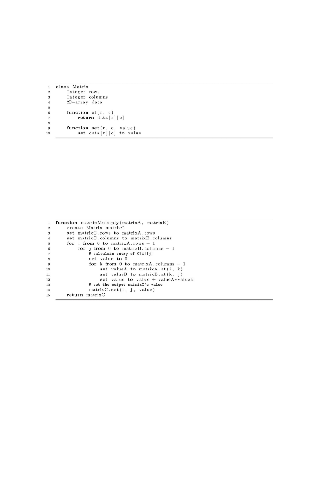
two convenience functions to access and set the values

of the matrix based on the row and column of the 2D

array.

With this structure for a Matrix class, we can

implement a matrix multiplication procedure. Below we

show the process of performing matrix multiplication on

two compatible matrices:

This function implements the matrix multiplication

procedure described above. On line 12, the new value of

the (i, j) entry in the result matrix is calculated. We see

that this involves a multiply operation and an addition

operation. On a typical processor, the multiply operation is

slower than addition. As we think about the complexity of

matrix multiplication, we will mainly consider the number

of multiplications. This is because as the matrices get

large, the cost associated with multiplication will dominate

the cost of addition. For this reason, we only consider the

number of multiplications.

So

how

many

multiplications

are

needed

for

matrix

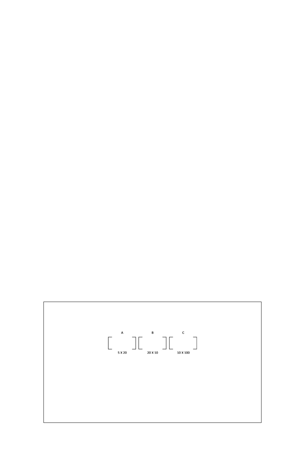
multiplication? The pattern above has a triple-nested loop.

This gives us a clue to the number of times the inner

code will run. As a result, we can expect the number of

multiplications to be equal to the number of times the

inner code will run. Let’s assume that matrix A has ra rows

and ca columns, and that matrix B, in a similar way, has rb

rows and cb columns. For A and B to be compatible

matrices, the value of ca would have to be equal to rb. We

know that the inner loop with index k runs a total of ca

times. This entire loop is executed once for every cb of B’s

columns (cb * ca). Finally, these two inner loops for j and k

would all run for every row in A, leading to multiplications

proportional to ra * ca * cb. This illustrates that as the size

of the matrices gets larger, the number of multiplications

grows quickly.

Why Order Matters

Now that we have seen how to multiply matrices together

and understand the computational cost, let’s consider just

why choosing to multiply in a specific order is important.

Suppose that we need to multiply three matrices—A, B,

and C—shown in the image below:

Figure 10.3

Multiplying them together could proceed with the

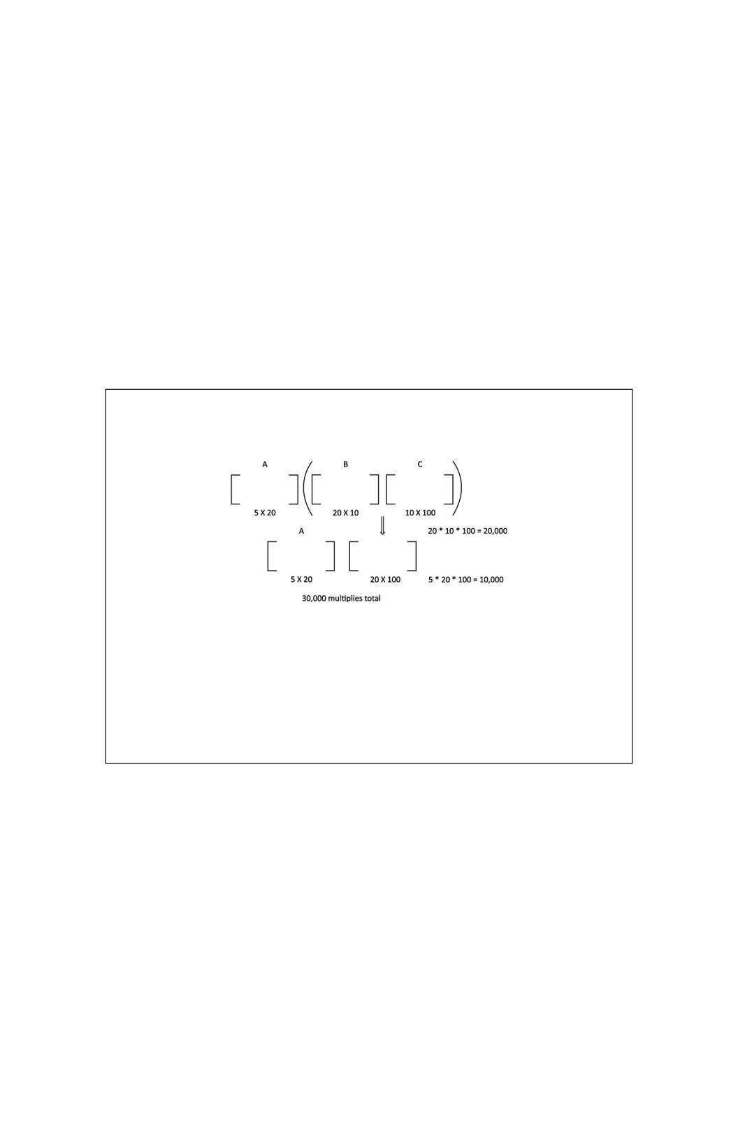
grouping (AB)C, where A and B are multiplied together

first, and then that result is multiplied by C. Alternatively, we

could group them as A(BC) and first multiply B by C, followed

by A multiplied by the result. Which would be better, or

would it even matter?

Let’s figure this out by first considering the A(BC)

grouping. The figure below illustrates this example. With

this grouping, calculating the BC multiplication yields

20,000 multiply operations. Multiplying A by this result

gives another 10,000 for a total of 30,000 multiply

operations.

Next, let’s consider the (AB)C grouping. The following

figure

shows a rough diagram of this calculation. The AB

matrix multiplication gives a cost of 1,000 multiply

operations. Then this result multiplied by C gives another

5,000. We now have a total of 6,000 multiply operations

for the (AB)C grouping over the other. This represents a

fivefold decrease in cost!

Figure 10.4

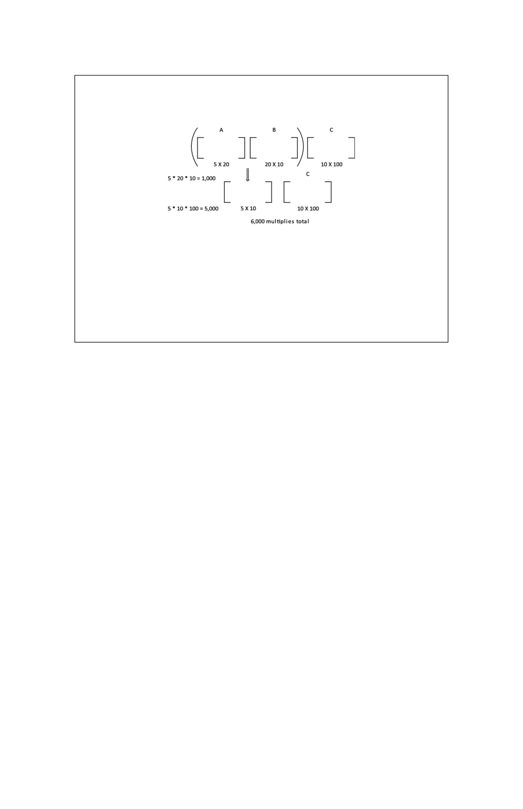
This example illustrates that the order of

multiplication definitely matters in terms of computational

cost. Additionally, as the matrices get larger, there could

be significant cost savings when we find an optimal

grouping for the multiplication sequence.

A Recursive Algorithm

for Optimal Matrix-Chain

Multiplication

We are interested in an algorithm for finding the optimal

ordering of matrix multiplication. This corresponds to

finding a grouping with a minimal cost. Suppose we have a

chain of 5 matrices, M

0

to M

4

. We could write their

dimensions as a list of 6 values. The 6 values come from

the fact that each sequential pair of matrices must be

compatible for multiplication to be possible. The figure

below shows this chain and gives the dimensions as a list.

Figure 10.5

An algorithm that minimizes the cost must find an

optimal split for the final two matrices. Let’s call these final

two matrices A and B. For the result to be optimal, then A

and B must both have resulted from an optimal subgrouping.

The possible splits would be

We need to evaluate these options by assessing

the cost of creating the A and B matrices (optimal

subproblems) as well as the cost of the final multiply, with

matrix A being multiplied by B. A recursive algorithm

would find the minimal cost by checking the minimum cost

among all splits. In the process of finding the cost of all

these four options for splits, we would need to calculate

the optimal splits for other sequences to find their optimal

groupings. This demonstrates the feature of optimal

substructure, the idea that an optimal solution could be

Figure 10.6

(M0) (M1 M2 M3 M4) = AB with a split after

position 0 (M0 M1) (M2 M3 M4) = AB with a split

after position 1 (M0 M1 M2) (M3 M4) = AB with a

split after position 2 (M0 M1 M2 M3) (M4) = AB

with a split after position 3.

built from optimal subproblems.

For the first grouping, we have A = M0 and B = (M1

M2 M3 M

4

). To calculate the cost of this split, it is

assumed that A and B have been constructed optimally.

This means that a recursive algorithm considering this split

must then make a recursive call to

find the minimal

grouping for (M1 M2 M3 M4) for the B matrix. This in

turn

would trigger another search for the optimal split among

(M

1

) (M2 M3 M4) (M1 M2) (M3 M4) and (M1 M2 M3) (M4). We

can also see

that this would trigger further calls to optimize each

sequence of 3 matrices and so on. You may be able to

imagine that this recursive process has a high branch

factor leading to an exponential runtime complexity in the

number of matrices. With n matrices, the runtime

complexity would be even worse than O(2n), exponential time. It

would follow an algorithm for calculating the Catalan

numbers at O(3n).

A general outline of the recursive algorithm would be

as follows. We will consider an algorithm to calculate the

minimal cost of multiplying a sequence of matrices starting at

some matrix identified by the start index and including the

ending matrix using an end index. The base case of the

algorithm is when start and end are equal. The cost of

multiplication of only one matrix is 0 as there is no

operation to perform. The recursive case calculates the cost

of splitting the sequence at some split position. There will be

n − 1 split positions to test when considering n matrices

where n = end − start

+ 1, and the recursive algorithm will need to find the

minimum of the options for the best split position.

To complete the recursive algorithm, we will

introduce a function to calculate the cost of the final

multiplication. This could be a simple multiplication of the

correct dimensions, but we will introduce and explain this

function to make the meaning clear and to simplify some

of the code (which would otherwise include a lot of

awkward indexing). The figure below illustrates what is

meant by the final multiplication:

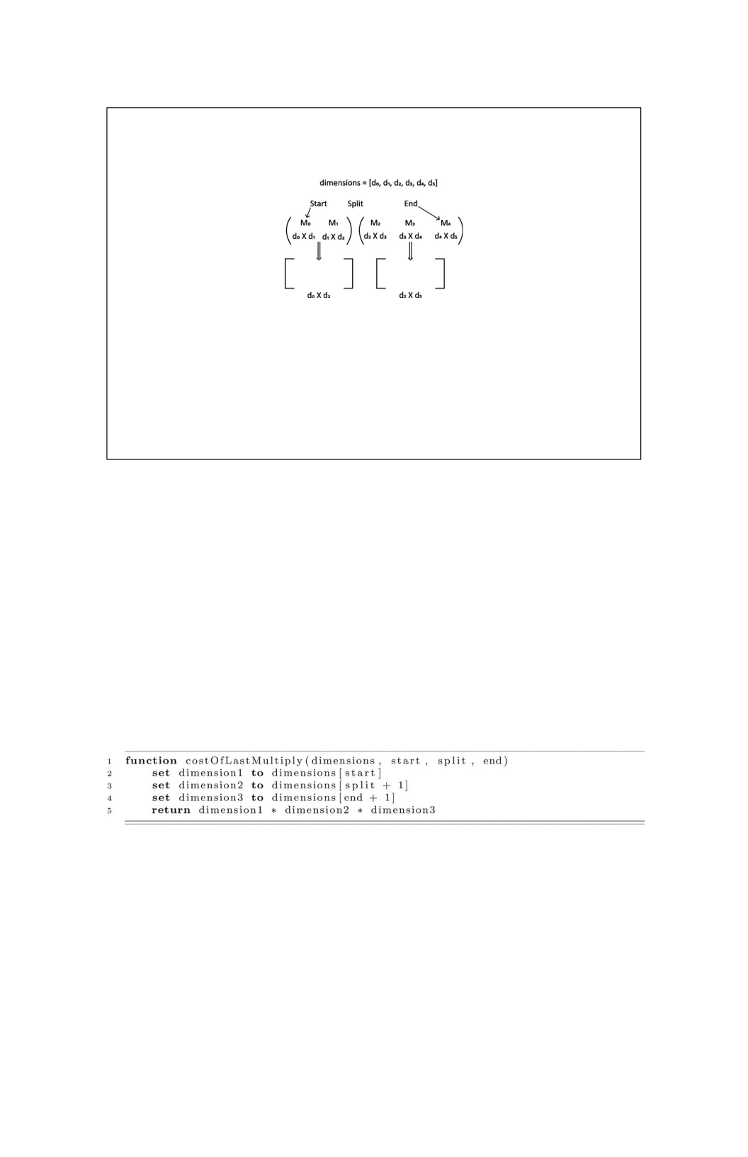
Suppose we are calculating the number of

multiplications for a split at index 1 (or just after M1). The

algorithm would have given the optimal cost for constructing

the left matrix and the right matrix, but we would still need to

calculate the cost of multiplying those together. The left

matrix would have dimensions of d0 by d2 and the right

matrix would have dimensions of d2 by d5. Using the

dimensions list and indexes for start, split, and end, we can

calculate this cost. The function below performs this operation

in a way that might make the meaning a little clearer. Notice

that for matrix i, the dimensions of that matrix are di by di+1.

With this helper function, we can now write the

recursive algorithm.

Figure 10.7

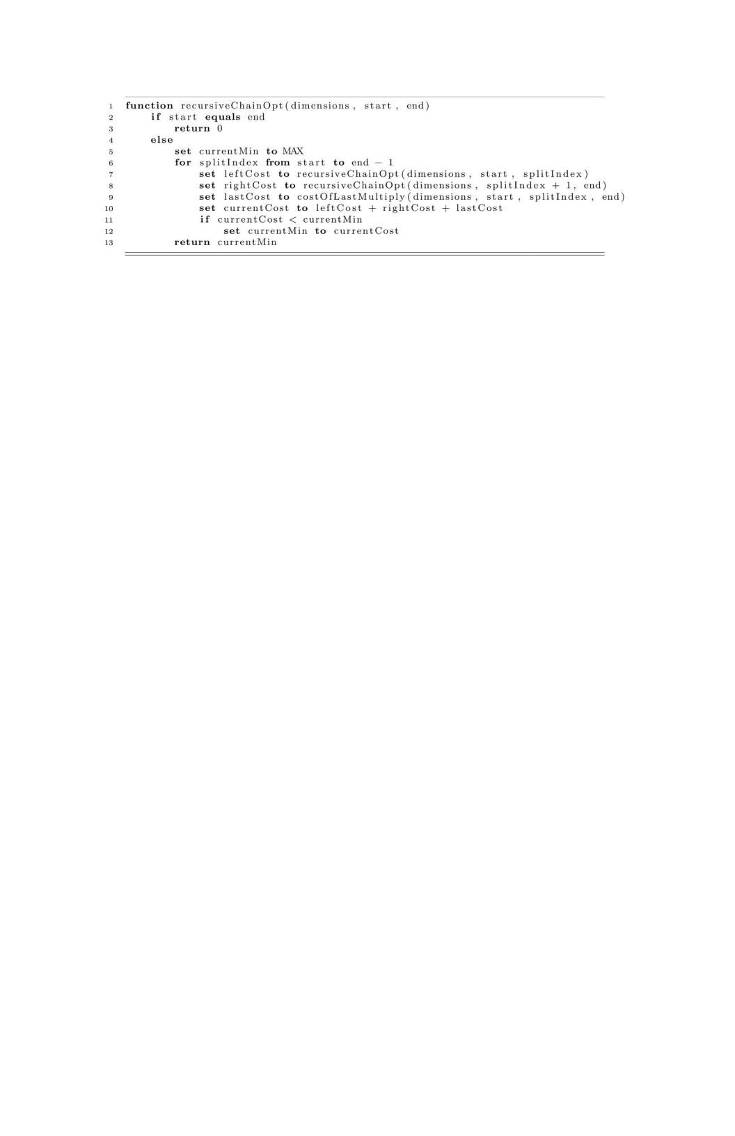
This algorithm only calculates an optimal cost, but

it could be modified to record the split indexes of the

optimal splits so that another process could use that

information. The optimal cost of multiplying all matrices in

the optimal grouping could be calculated with a call to

recursiveChainOpt(dimensions, 0, 4). This algorithm, while

correct, suffers from exponential time complexity. This is

the type of situation where dynamic programming can

help.

Requirements for Applying

Dynamic Programming

There are two main requirements for applying dynamic

programming. First, a problem must exhibit the property

known as optimal substructure. This means that an

optimal solution to the problem is constructed from

optimal solutions to the subproblems. We will see an

example of this soon. The second property is called

overlapping subproblems. This means that subproblems

are shared. We saw this in our Fibonacci example.

Optimal Matrix Chain Multiplication

A classic application of dynamic programming concerns

the optimal multiplication order for matrices. Consider the

sequence of matrices {M1, M2, M3, M4}. There are several

ways to multiply these together. These ways correspond

to the number of distinct ways to parenthesize the matrix

multiplication order. For the mathematically curious, the

Catalan numbers give the total number of possible ways.

For example, one way to group these would be (M

1

M2) (M3

M4). Another way could be M1 ((M2 M3) M4). Any grouping

leads to the same final result, but the number of multiply

operations of the overall calculation could differ greatly

with different groupings. To understand this idea, let’s

review matrix multiplication.

Matrix

Multiplication

Review

Matrix multiplication is an operation that multiplies and adds the

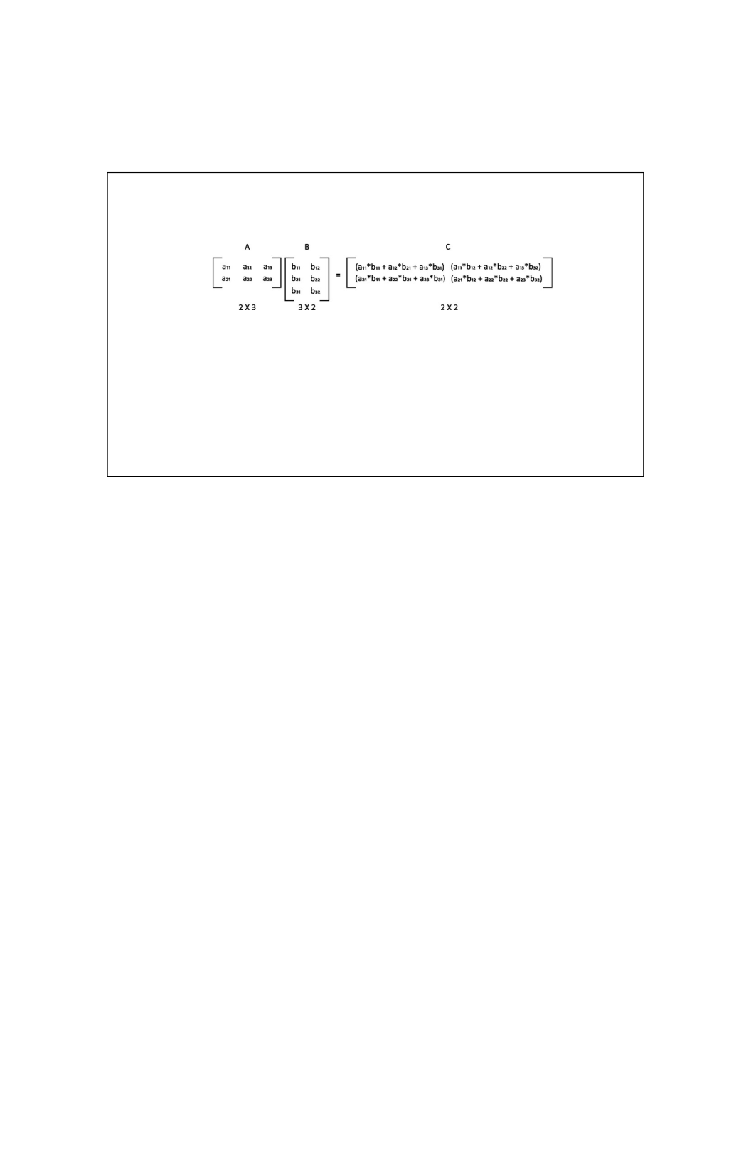
rows of one matrix with the columns of another matrix.

Below is an example:

Here we have the matrix A and the matrix B. A is a

2-by-3 matrix (2 rows and 3 columns), and B is a 3-by-2

matrix (3 rows

and 2 columns). The multiplication of AB is

compatible, which means

the number of columns of A is

equal to the number of rows in the second matrix, B. When

two compatible matrices are multiplied, their result has a

structure where the number of rows equals the number of

rows in the first matrix and the number of columns equals

the number of columns in the second matrix. The process

is the same for compatible matrices of any size.

Implementing

Matrix

Multiplication

Now let’s consider an algorithm for matrix multiplication.

To simplify things, let’s assume we have a Matrix class or

data structure that has a two-dimensional (2D) array.

Another way to think of a 2D array is as an array of

arrays. We could also think of this as a table with rows

and columns. The structure below gives a general example

of a Matrix class. Within this class, we also have

Figure 10.2

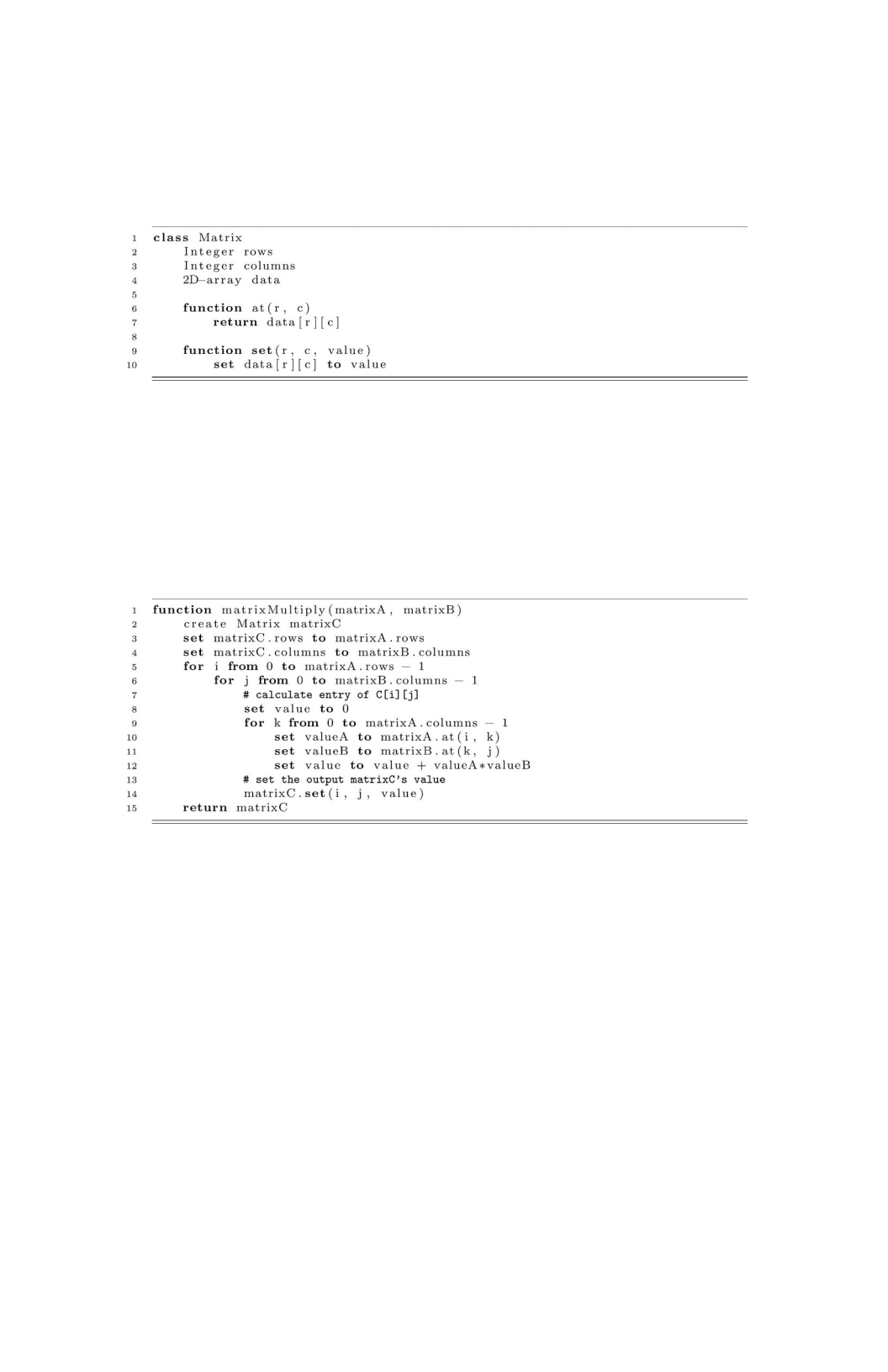
two convenience functions to access and set the values

of the matrix based on the row and column of the 2D

array.

With this structure for a Matrix class, we can

implement a matrix multiplication procedure. Below we

show the process of performing matrix multiplication on

two compatible matrices:

This function implements the matrix multiplication

procedure described above. On line 12, the new value of

the (i, j) entry in the result matrix is calculated. We see

that this involves a multiply operation and an addition

operation. On a typical processor, the multiply operation is

slower than addition. As we think about the complexity of

matrix multiplication, we will mainly consider the number

of multiplications. This is because as the matrices get

large, the cost associated with multiplication will dominate

the cost of addition. For this reason, we only consider the

number of multiplications.

So

how

many

multiplications

are

needed

for

matrix

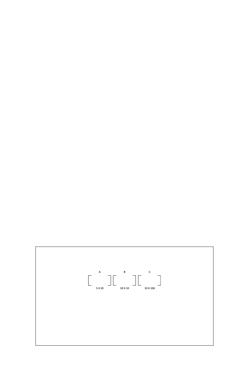
multiplication? The pattern above has a triple-nested loop.

This gives us a clue to the number of times the inner

code will run. As a result, we can expect the number of

multiplications to be equal to the number of times the

inner code will run. Let’s assume that matrix A has ra rows

and ca columns, and that matrix B, in a similar way, has rb

rows and cb columns. For A and B to be compatible

matrices, the value of ca would have to be equal to rb. We

know that the inner loop with index k runs a total of ca

times. This entire loop is executed once for every cb of B’s

columns (cb * ca). Finally, these two inner loops for j and k

would all run for every row in A, leading to multiplications

proportional to ra * ca * cb. This illustrates that as the size

of the matrices gets larger, the number of multiplications

grows quickly.

Why Order Matters

Now that we have seen how to multiply matrices together

and understand the computational cost, let’s consider just

why choosing to multiply in a specific order is important.

Suppose that we need to multiply three matrices—A, B,

and C—shown in the image below:

Figure 10.3

Multiplying them together could proceed with the

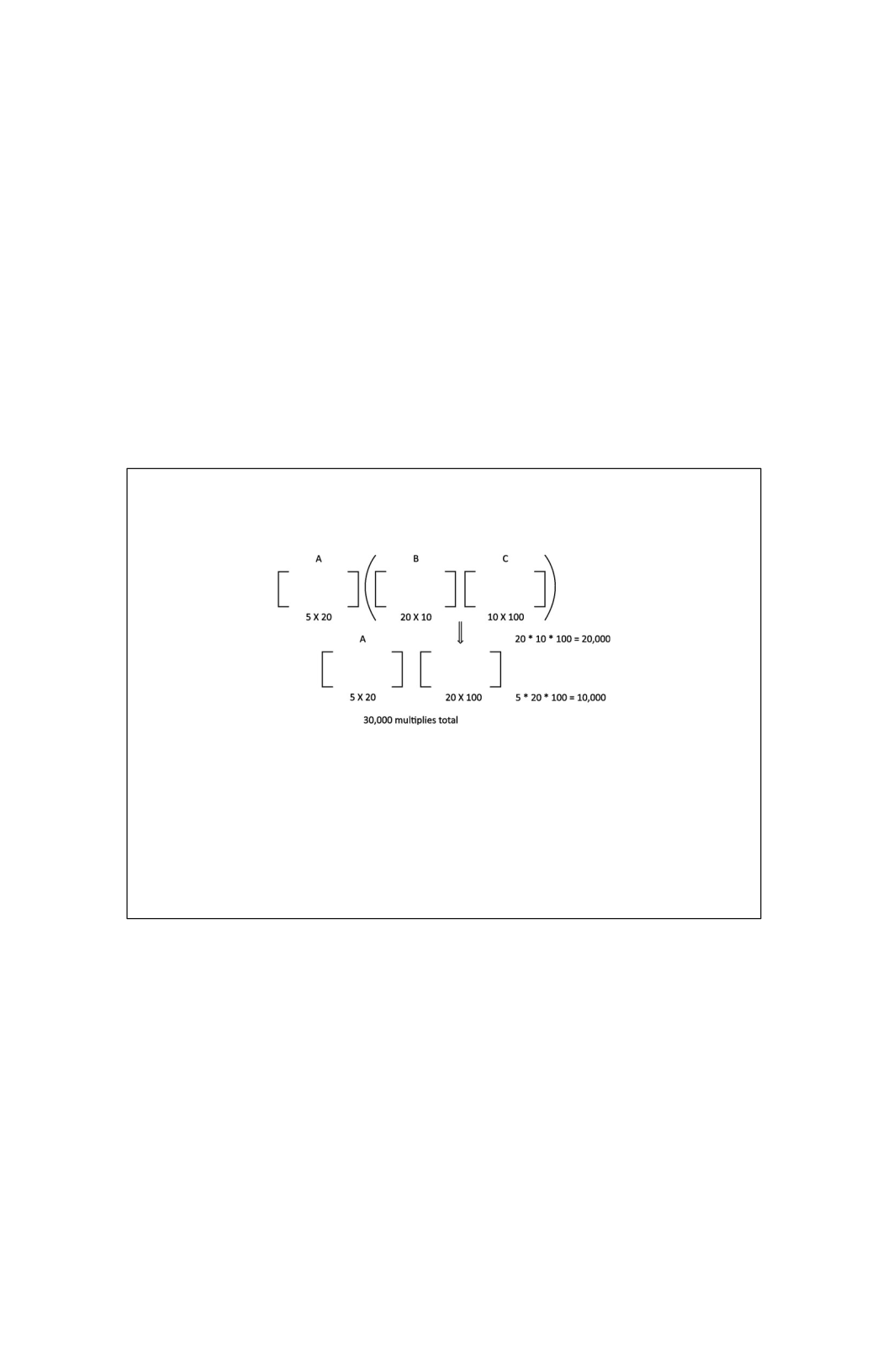
grouping (AB)C, where A and B are multiplied together

first, and then that result is multiplied by C. Alternatively, we

could group them as A(BC) and first multiply B by C, followed

by A multiplied by the result. Which would be better, or

would it even matter?

Let’s figure this out by first considering the A(BC)

grouping. The figure below illustrates this example. With

this grouping, calculating the BC multiplication yields

20,000 multiply operations. Multiplying A by this result

gives another 10,000 for a total of 30,000 multiply

operations.

Next, let’s consider the (AB)C grouping. The following

figure

shows a rough diagram of this calculation. The AB

matrix multiplication gives a cost of 1,000 multiply

operations. Then this result multiplied by C gives another

5,000. We now have a total of 6,000 multiply operations

for the (AB)C grouping over the other. This represents a

fivefold decrease in cost!

Figure 10.4

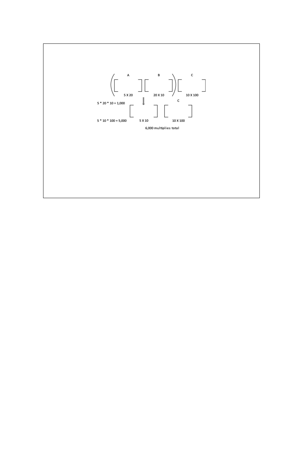
This example illustrates that the order of

multiplication definitely matters in terms of computational

cost. Additionally, as the matrices get larger, there could

be significant cost savings when we find an optimal

grouping for the multiplication sequence.

A Recursive Algorithm

for Optimal Matrix-Chain

Multiplication

We are interested in an algorithm for finding the optimal

ordering of matrix multiplication. This corresponds to

finding a grouping with a minimal cost. Suppose we have a

chain of 5 matrices, M

0

to M

4

. We could write their

dimensions as a list of 6 values. The 6 values come from

the fact that each sequential pair of matrices must be

compatible for multiplication to be possible. The figure

below shows this chain and gives the dimensions as a list.

Figure 10.5

An algorithm that minimizes the cost must find an

optimal split for the final two matrices. Let’s call these final

two matrices A and B. For the result to be optimal, then A

and B must both have resulted from an optimal subgrouping.

The possible splits would be

We need to evaluate these options by assessing

the cost of creating the A and B matrices (optimal

subproblems) as well as the cost of the final multiply, with

matrix A being multiplied by B. A recursive algorithm

would find the minimal cost by checking the minimum cost

among all splits. In the process of finding the cost of all

these four options for splits, we would need to calculate

the optimal splits for other sequences to find their optimal

groupings. This demonstrates the feature of optimal

substructure, the idea that an optimal solution could be

Figure 10.6

(M0) (M1 M2 M3 M4) = AB with a split after

position 0 (M0 M1) (M2 M3 M4) = AB with a split

after position 1 (M0 M1 M2) (M3 M4) = AB with a

split after position 2 (M0 M1 M2 M3) (M4) = AB

with a split after position 3.

built from optimal subproblems.

For the first grouping, we have A = M0 and B = (M1

M2 M3 M

4

). To calculate the cost of this split, it is

assumed that A and B have been constructed optimally.

This means that a recursive algorithm considering this split

must then make a recursive call to

find the minimal

grouping for (M1 M2 M3 M4) for the B matrix. This in

turn

would trigger another search for the optimal split among

(M

1

) (M2 M3 M4) (M1 M2) (M3 M4) and (M1 M2 M3) (M4). We

can also see

that this would trigger further calls to optimize each

sequence of 3 matrices and so on. You may be able to

imagine that this recursive process has a high branch

factor leading to an exponential runtime complexity in the

number of matrices. With n matrices, the runtime

complexity would be even worse than O(2n), exponential time. It

would follow an algorithm for calculating the Catalan

numbers at O(3n).

A general outline of the recursive algorithm would be

as follows. We will consider an algorithm to calculate the

minimal cost of multiplying a sequence of matrices starting at

some matrix identified by the start index and including the

ending matrix using an end index. The base case of the

algorithm is when start and end are equal. The cost of

multiplication of only one matrix is 0 as there is no

operation to perform. The recursive case calculates the cost

of splitting the sequence at some split position. There will be

n − 1 split positions to test when considering n matrices

where n = end − start

+ 1, and the recursive algorithm will need to find the

minimum of the options for the best split position.

To complete the recursive algorithm, we will

introduce a function to calculate the cost of the final

multiplication. This could be a simple multiplication of the

correct dimensions, but we will introduce and explain this

function to make the meaning clear and to simplify some

of the code (which would otherwise include a lot of

awkward indexing). The figure below illustrates what is

meant by the final multiplication:

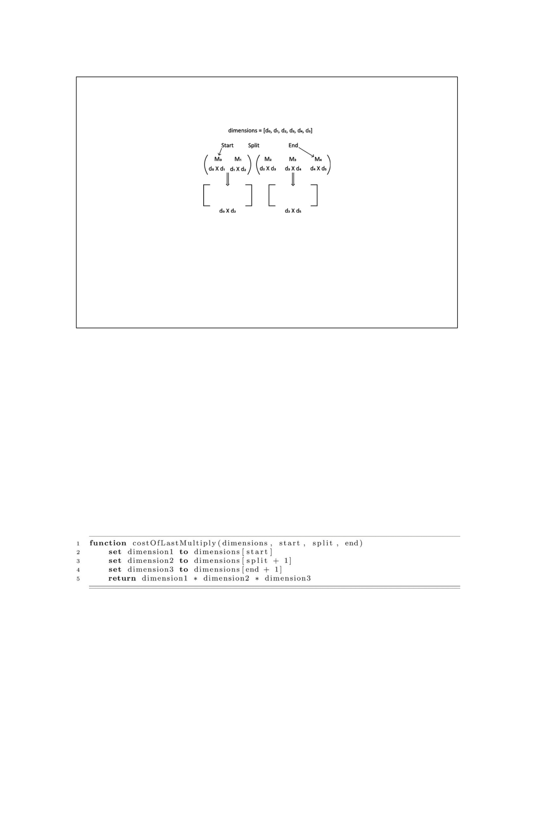
Suppose we are calculating the number of

multiplications for a split at index 1 (or just after M1). The

algorithm would have given the optimal cost for constructing

the left matrix and the right matrix, but we would still need to

calculate the cost of multiplying those together. The left

matrix would have dimensions of d0 by d2 and the right

matrix would have dimensions of d2 by d5. Using the

dimensions list and indexes for start, split, and end, we can

calculate this cost. The function below performs this operation

in a way that might make the meaning a little clearer. Notice

that for matrix i, the dimensions of that matrix are di by di+1.

With this helper function, we can now write the

recursive algorithm.

Figure 10.7

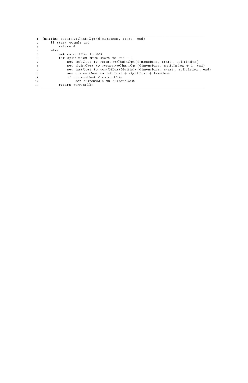
This algorithm only calculates an optimal cost, but

it could be modified to record the split indexes of the

optimal splits so that another process could use that

information. The optimal cost of multiplying all matrices in

the optimal grouping could be calculated with a call to

recursiveChainOpt(dimensions, 0, 4). This algorithm, while

correct, suffers from exponential time complexity. This is

the type of situation where dynamic programming can

help.

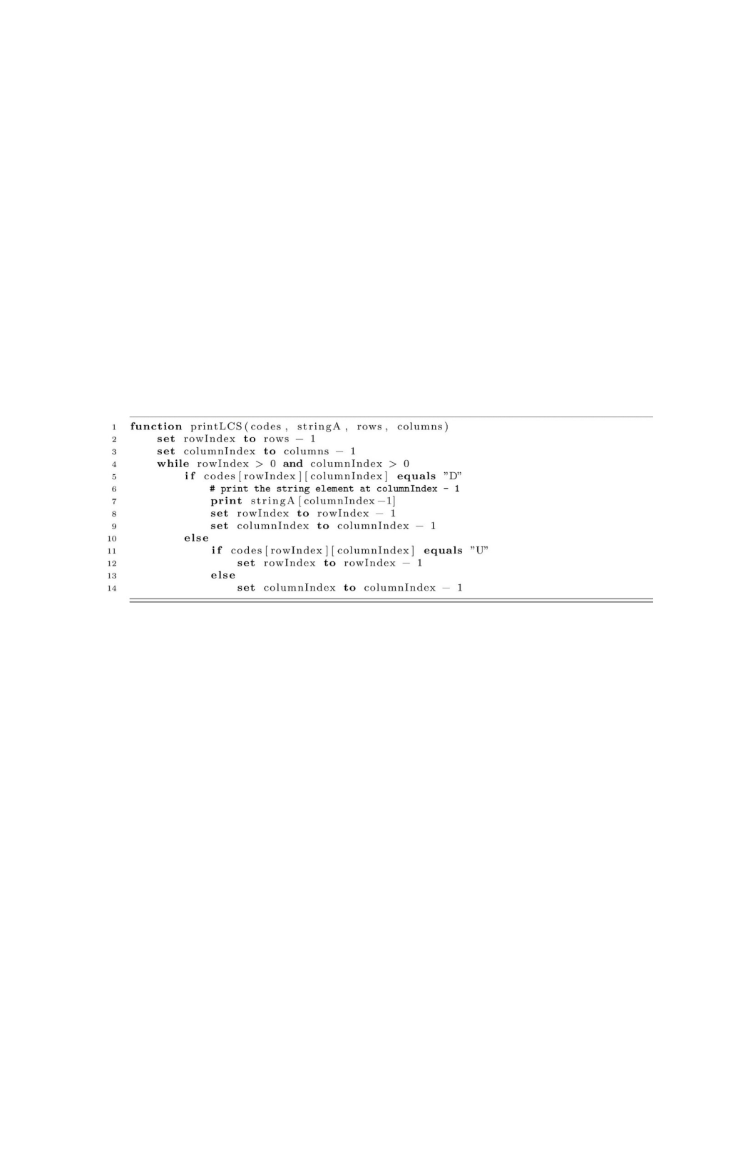
Extracting

the

LCS

String

Before we move on to the complexity analysis, let’s

discuss how to read the LCS from the codes table.

Depending on the design of your algorithm, you may be

able to extract the LCS just from the strings and the

lengths table, and the codes table could be omitted from

the algorithm completely. We would like to keep things

simple though, so we will just use the codes table. The

algorithm below shows one method for printing the LCS

string (in reverse order):

Complexity of the Dynamic

Programming

Algorithm

Now that we have seen the algorithm and an example,

let’s consider the time complexity of the algorithm. The

nested loops for the A and B indexes should be a clue. In

the worst case, all increasing subsequences of each input

string need to be compared. The algorithm fills every cell

of the n-by-m table (ignoring the first row and column of

zeros, which are initialized with a minor time cost). This

gives us n * m cells, so the complexity of the algorithm

would be considered O(mn). It might be reasonable to

assume that m and n are roughly equal in size. This would

lead to a time complexity of O(n

2

). This represents a huge

cost savings over the O(2n) time cost of the recursive

algorithm.

The space complexity is straightforward to

calculate. We need two tables, each of size n+1 by m+1.

So the space complexity would also be O(m*n), or,

assuming m is roughly equal to n, O(n

2

).

Students also viewed