


Chapter 4 : SPS Problems
Paul Kunesh
School of Business, Liberty University
BUSI820: Quantitative Research Methods (D04)
Dr. David Danley
November 9, 2025
Author Note
Paul Kunesh
I have no known conflict of interest to disclose.
Correspondence concerning this article should be addressed to Paul Kunesh.
Email: [email protected]

BUSI820: Quantitative Research Methods (D04)
Table of Contents
4.1 Skewness....................................................................................................................................2
Figure 1 - Skewness.........................................................................................................................2
4.2 Steam and Leaf Plot...................................................................................................................3
Figure 2 – Stem and Leaf Plot.........................................................................................................4
4.3 Nominal Variables.....................................................................................................................5
Figure 3 - Sex at Birth.....................................................................................................................5
Figure 4 - Marital Status..................................................................................................................5
Figure 5 – Does Subject have Children...........................................................................................6
Figure 6 Television Shows-Sitcoms................................................................................................6
Figure 7 Television Shows – Sports................................................................................................7
Figure 8 Television Shows – Movies..............................................................................................7
Figure 9 Television Shows – News Shows......................................................................................7
4.4 Box Plots....................................................................................................................................8
Figure 10 Box Plot - Student Height...............................................................................................9
Figure 11 Box Plot – Hours of Study..............................................................................................9
References......................................................................................................................................10
1 November 9, 2025
BUSI820: Quantitative Research Methods (D04)
4.1 Skewness
Q. For the variables with five or more ordered levels, compute the skewness. Describe the
results. Which variables in the dataset are approximately normally distributed/scale? Which
ones are ordered but not normal?
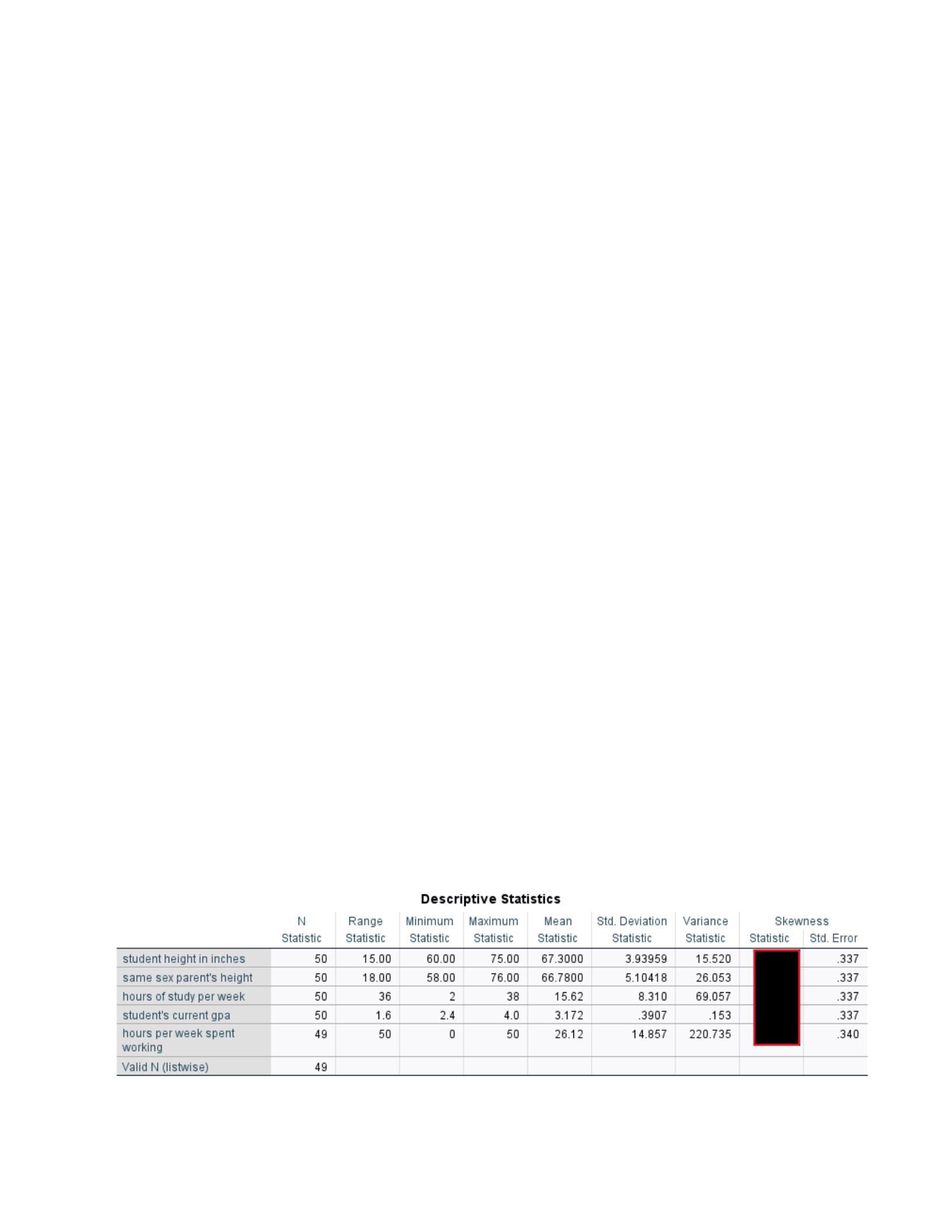
Skewness values were calculated for all variables with five or more ordered levels to
assess their distribution shapes. The results in Figure 1 indicate that student height in inches
(skewness = 0.163), same-sex parent’s height (skewness = 0.333), and student’s current GPA
(skewness = 0.147) is approximately normally distributed, showing that their values are
relatively balanced around the mean. Hours per week spent working (skewness = –0.516)
displays a slight negative skew, suggesting that a greater number of students work longer hours,
although the distribution is still close to normal. In contrast, hours of study per week (skewness =
0.950) demonstrates a moderate positive skew, indicating that most students report fewer study
hours, with only a few studying significantly more. The results show that the height and GPA
variables can be considered approximately normal, while hours of study per week are ordered
but not normally distributed. According to Morgan et al. (2020), variables with skewness values
between –0.5 and +0.5 are considered approximately normal, while values outside this range
indicate varying degrees of skewness.
Figure 1 - Skewness
2 November 9, 2025

BUSI820: Quantitative Research Methods (D04)
4.2 Steam and Leaf Plot
Q. Do a stem-and-leaf plot for the same-sex parent’s height split by sex at birth. Discuss the
plots.
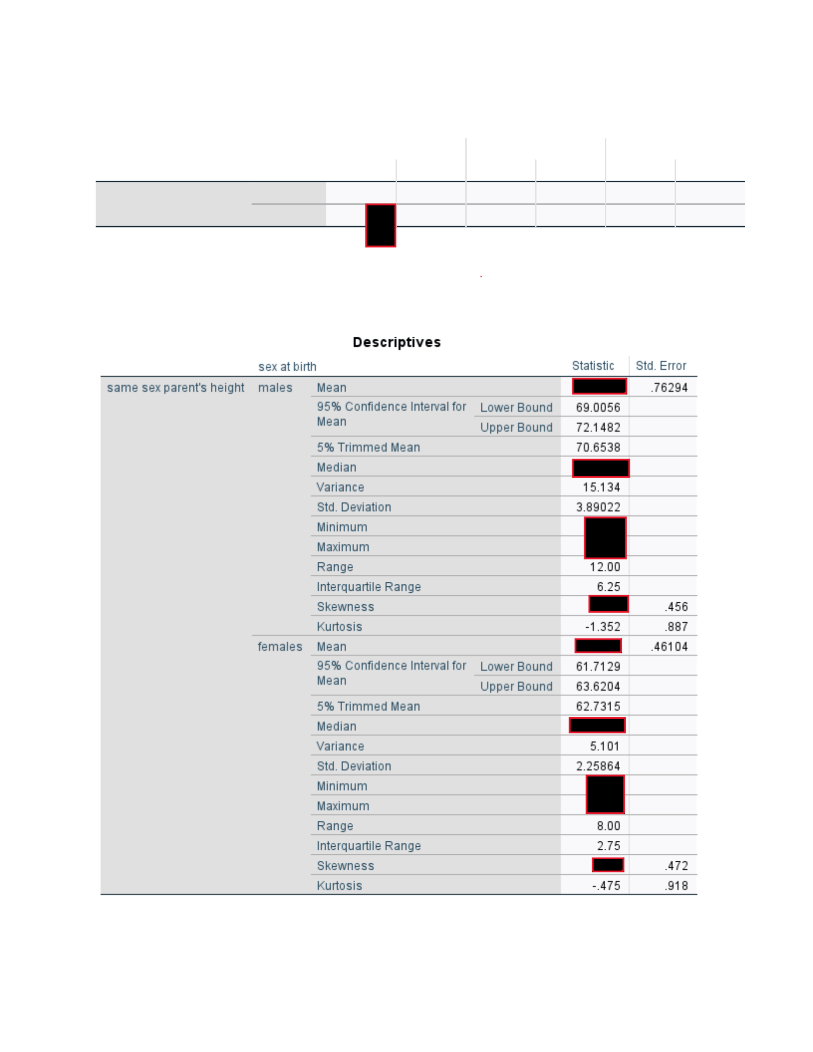
The stem-and-leaf plots for the same-sex parent’s height were generated separately for
males and females to compare the distribution of height values by sex at birth. The descriptive
results in Figure 2 show distinct patterns between the two groups. For male students, the same-
sex parent’s height values range from 64 to 76 inches, with a mean of 70.58 inches and a median
of 72 inches. The distribution appears symmetrical (skewness = –0.369), indicating that most
male parents’ heights cluster around the 70–72-inch range, with relatively few cases at the lower
and higher ends. The moderate spread (standard deviation = 3.89) and range of 12 inches suggest
greater variability among male parents’ heights. For female students, the same-sex parent’s
height values range from 58 to 66 inches, with a mean of 62.67 inches and a median of 62.5
inches. The distribution is also approximately symmetrical (skewness = –0.139) but shows less
variability than that of males, with a smaller standard deviation (2.26) and a narrower range of 8
inches. The stem-and-leaf plot for females would likely show a tight clustering of scores around
the center (61–64 inches), indicating that female parents’ heights are more consistent across
cases. The stem-and-leaf plots reveal that male parents tend to be taller on average and exhibit
more variation in height, while female parents’ heights are shorter and more concentrated around
the mean. Both groups show roughly normal distributions without extreme outliers. These
findings align with general biological expectations of height differences by sex.
3 November 9, 2025
BUSI820: Quantitative Research Methods (D04)
Case Processing Summary for Figure 2
sex at
birth
Cases
Valid Missing Total
N Percent N Percent N Percent
same sex parent's
height
males 26 100.0% 0 0.0% 26 100.0%
females 24 100.0% 0 0.0% 24 100.0%
Figure 2 – Stem and Leaf Plot
4 November 9, 2025
BUSI820: Quantitative Research Methods (D04)
4.3 Nominal Variables
Q. Which variables are nominal? Run Frequencies for the nominal variables and other
variables with fewer than five levels. Comment on the results.
In this dataset, the variables sex at birth, marital status, does subject have children, and
television shows - sitcoms, movies, sports, news shows are nominal because they represent
categories without numerical meaning or order.
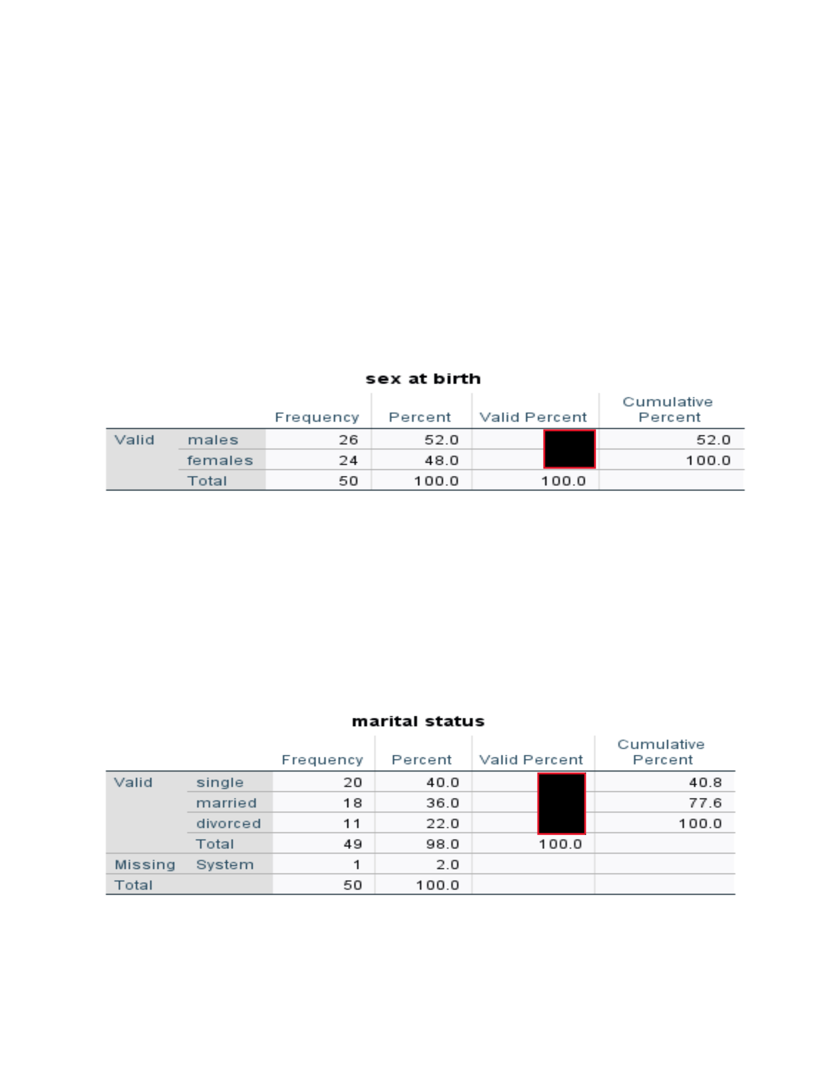
Figure 3 - Sex at Birth
The frequency analysis in Figure 3 shows that 52% of participants were male and 48%
were female, indicating an almost equal distribution between the two groups. This balanced
representation suggests that both sexes are well represented in the dataset, which helps ensure
fairness and comparability in further statistical analyses (Morgan et al., 2020).
Figure 4 - Marital Status
The variable marital status is nominal, as it classifies participants into categories without
any numerical or ranked order. The frequency results show that 40.8% of participants were
5 November 9, 2025
BUSI820: Quantitative Research Methods (D04)
single, 36.7% were married, and 22.4% were divorced. Only one case (2%) was missing data.
These results indicate that most participants in the dataset are single, with married individuals
making up a slightly smaller portion and divorced individuals representing the smallest group.
The relatively balanced distribution across categories suggests a diverse sample in terms of
marital background, which can enhance the representativeness of the study’s findings (Morgan et
al., 2020).
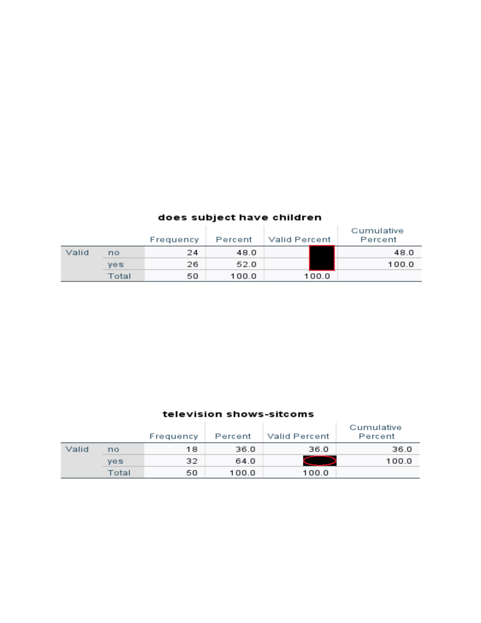
Figure 5 – Does Subject have Children
The frequency results indicate that 48% of participants reported not having children,
while 52% reported having at least one child. This distribution suggests that more participants
have children which may align with the demographic pattern observed in the marital status and
age group variables, where many participants identified as younger or single adults.
Figure 6 Television Shows-Sitcoms
6 November 9, 2025
BUSI820: Quantitative Research Methods (D04)
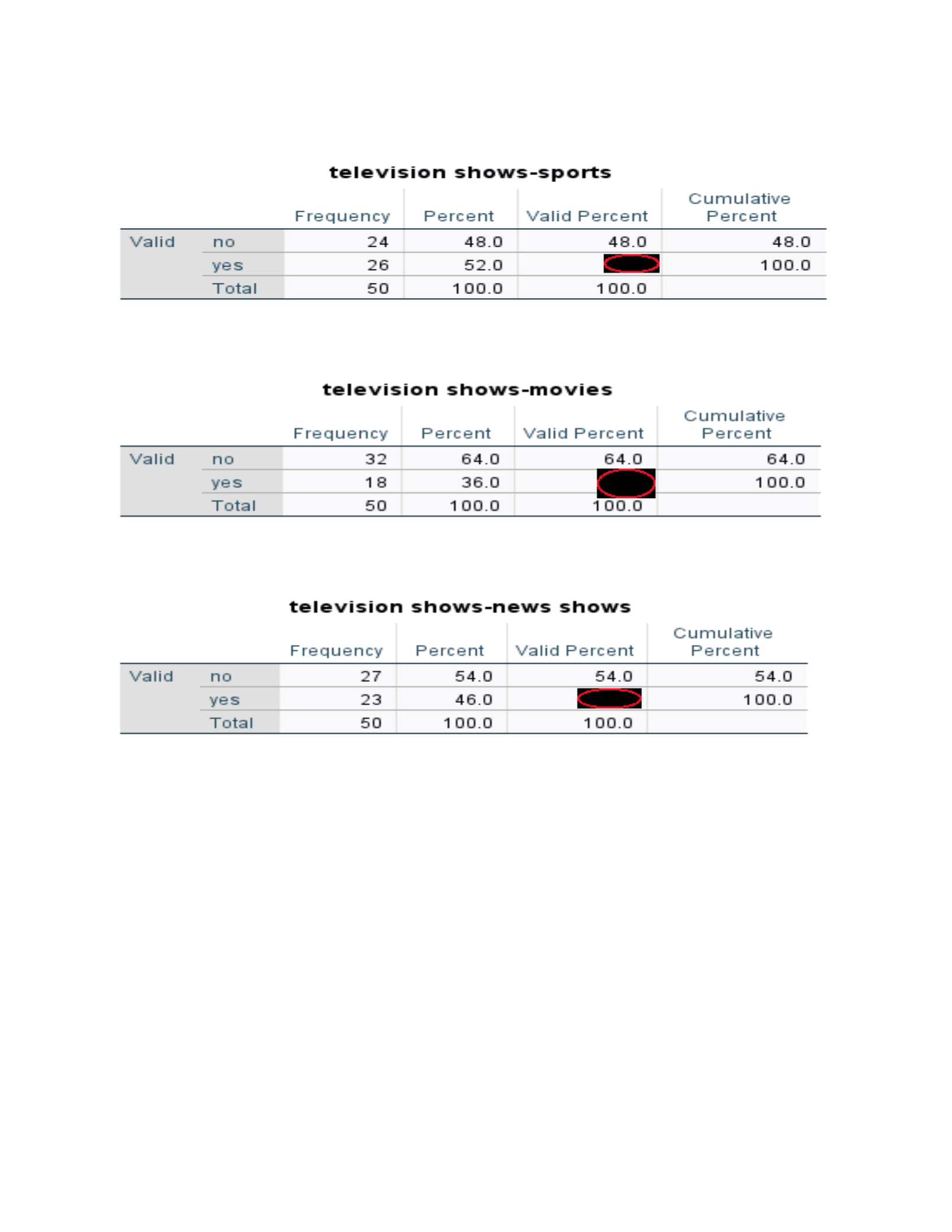
Figure 7 Television Shows – Sports
Figure 8 Television Shows – Movies
Figure 9 Television Shows – News Shows
The results of the data in Figures 6-9 suggest that sitcoms and sports are the most
frequently watched types of programming among students, with approximately 58% of
participants reporting that they regularly view these genres. In contrast, fewer participants
indicated watching movies or news programs, which may reflect generational differences in
media preferences or the growing popularity of streaming entertainment among younger adults.
7 November 9, 2025

BUSI820: Quantitative Research Methods (D04)
4.4 Box Plots
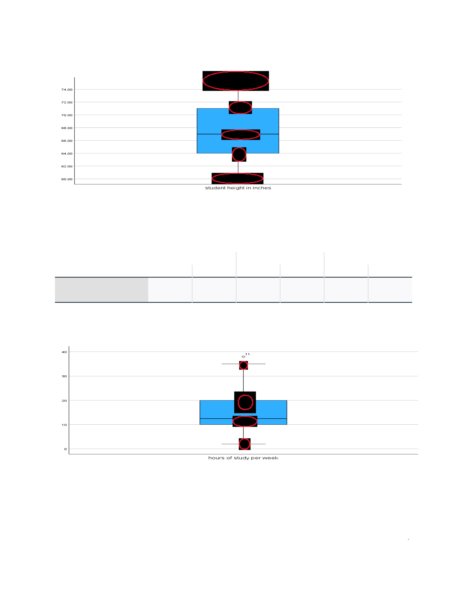
Q. Do boxplots for student height and for hours of study. Compare the two plots.
After examining the frequency table, it was confirmed that all participants had provided
responses. The median height of participants in Figure 10 is 67.3 inches, with a range from 60 to
75 inches. The most frequently occurring height is 64 inches, suggesting a relatively typical
distribution of student heights. As displayed in Figure 11 the number of hours spent studying
each week indicates an approximately normal distribution. However, the corresponding
histogram reveals a right-skewed distribution, with the highest concentrations of study hours not
centered around the mean. From the frequency table the average number of study hours per week
is 15.62, ranging from 2 to 38 hours. Most students reported studying between 10 and 12 hours
per week, while 2 hours per week was the next most frequently reported. The analysis of student
heights and study hours provides insight into both typical and extreme values within the sample,
helping to understand patterns in student behavior and characteristics (Morgan et al., 2020).
Case Processing Summary for Figure 10
Cases
Valid Missing Total
N Percent N Percent N Percent
student height in
inches
50 100.0% 0 0.0% 50 100.0%
8 November 9, 2025
BUSI820: Quantitative Research Methods (D04)
Figure 10 Box Plot - Student Height
Case Processing Summary for Figure 11
Cases
Valid Missing Total
N Percent N Percent N Percent
hours of study per
week
50 100.0% 0 0.0% 50 100.0%
Figure 11 Box Plot – Hours of Study
9 November 9, 2025

BUSI820: Quantitative Research Methods (D04)
References
Morgan, G., Leech, N., Gloeckner, G., Barrett, K. (2020). IBM SPSS for Introductory Statistics
(6th Ed.). New York, NY
10 November 9,
2025

