SPSS HOMEWORK: ONE-WAY ANOVA ASSIGNMENT
Katherine Crisco
School of Behavioral Science, Liberty University
PSYC 355: Statistics in Psychology
Dr. Haynes
SEPTEMBER 8, 2025
Problem Set 1: The One-way ANOVA
Research Scenario: A group of clinical psychologists conducts a randomized clinical trial
examining psychosocial and pharmaceutical treatments, alone or in combination, for Social
Anxiety Disorder (SAD). Participants who have been diagnosed with SAD are randomly assigned
to one of three treatment groups: cognitive behavioral therapy (CBT); Paxil ® (a common SSRI
prescribed to patients with SAD); and CBT + Paxil ®. The participants are assessed after 6 months
of treatment using the Social Avoidance and Distress Scale (SADS; Watson and Friend, 1969),
where higher scores indicate higher levels of social anxiety. Their SADS scores are in the table
below.
Using this table, enter the data into a new SPSS data file and run a one-way ANOVA to test
whether there is a difference in SADS scores between the three treatments. Remember to put
your initials within any and all variable names. Create a boxplot to show the difference
between the groups. Follow the directions below the table to complete the homework.
CBT Paxil ® CBT + Paxil ®
16
18
25
20
21
16
19
19
17
25
18
14
12
23
19
27
12
12
14
25
18
16
20
13
1. Paste SPSS output. (10 pts)
Between-Subjects Factors
Value Label
N
Treatment Group 1 CBT 8
2Paxil 8
3CBT +
Paxil
8
Descriptive Statistics
Dependent Variable: Soical Avoidance and
Distress Scale Score
Treatmen
t
Group
Mea
n
Std
.
Deviatio
n N
CBT 19.
2
5
2.915 8
Paxil 19.
3
8
5.263 8
CBT +
Paxil
16.
8
6
4.562 8
Total 18.
5
7
4.305 24
Tests of Between-Subjects Effects
Dependent Variable: Soical Avoidance and Distress Scale Score
Source
Type III
Sum of
Squares df
Mean
Squar
e F
Sig
.
Partial
Eta
Square
d
Correcte 29.420 2 14.7 .7 .4 .07
d Model
a1
0
7
8
7
3
2
Intercep
t
7835.5
9
2
1 7835
.
59
2
4
1
4.
3
2
7
<.0
0
1
.95
4
XX_Trea
tment
29.420 2 14.7
1
0
.7
7
8
.4
7
3
.07
2
Error 378.23
2
2
0
18.9
1
2
Total 8335.0
0
0
2
3
Correcte
d Total
407.65
2
2
2
a. R Squared = .072 (Adjusted R Squared = -.021)
Case Processing Summary
Cases
Treatm
ent
Group
Valid
N
Perce
nt N
Missing Perce
nt N
Total
Perce
nt
Soical
Avoidan
ce and
Distress
Scale
Score
CBT 8 100.0
%
0 0.0% 8 100.0
%
Paxil 8 100.0
%
0 0.0% 8 100.0
%
CBT +
Paxil
7 100.0
%
0 0.0% 7 100.0
%
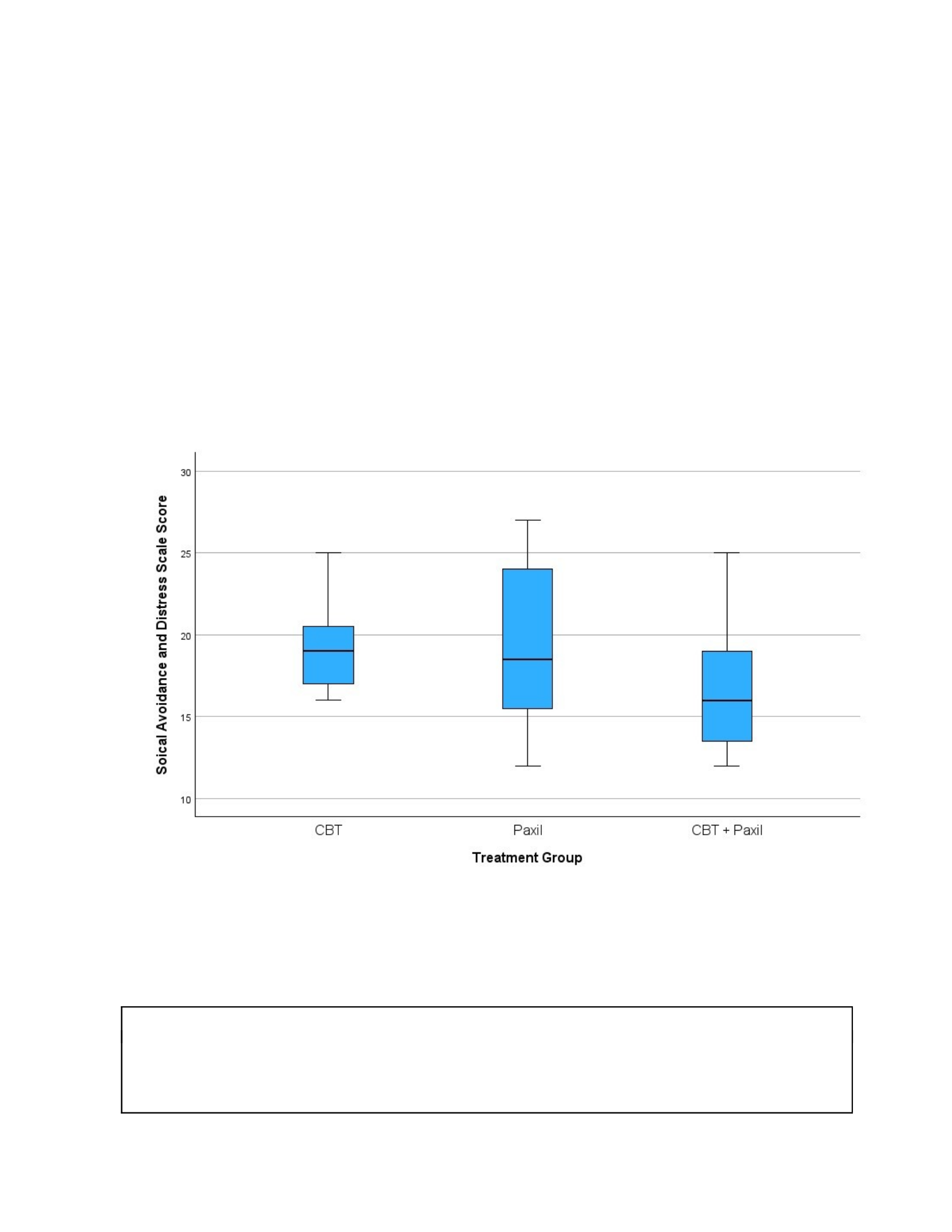
2. Write an APA-style Results section based on your analysis. Include your boxplot as an
APA-style Figure, with figure number and title, as demonstrated in the Results Section
presentation. (Results = 12 pts; Figure = 8 pts)
A one-way ANOVA test was conducted along with an analysis of variance to investigate
further and look into the possible effects of three different types of treatment, which were
CBT, Paxil, and the combination of both CBT+Paxil, and these treatments were to help
people who suffer from social anxiety disorder, which is known as SAD. The description of
statistics for each treatment group can be found in the boxplot below. The overall results of
the one-way ANOVA test conveyed that there is no big and major difference between the
treatment types on the Scores XX_SAD, which is F(2,21), which equals 1.318, p=.289, and
n²=.112. In addition, the post hoc test did not show any significant difference between the
different types of treatments. The overall results and findings did not show any significant
difference between the treatment groups.
Problem Set 2: The One-way ANOVA
Research Scenario: A developmental psychologist is studying the progression of object
permanence (the understanding that an object still exists even if it’s out of sight). She tests
three groups of infants – ten who are 9 months old, eight who are 12 months old, and ten who
are 15 months old. She presents each of the infants with 10 trials. On each trial, a toy is first
shown to the child and then covered with a piece of cloth. The infant demonstrates object
permanence if he or she continues to look for the object while it is still covered. Each infant is
given a score for the number of trials (out of 10) on which he or she shows object permanence.
Is there a significant difference between the groups on demonstrations of object permanence?
Using this table, enter the data into a new SPSS data file and run a one-way ANOVA to test
whether there is a difference in object permanence scores among the three age groups.
Remember to put your initials within any and all variable names. Create a boxplot to show
the difference between the groups. Follow the directions below the table to complete the
homework.
9 months 12 months 15 months
8 10 10
3
4
6
5
4
9
2
0
1
5
6
7
6
5
10
3
8
9
9
8
7
9
10
6
9
1. Paste SPSS output. (10 pts)
Between-Subjects Factors
Value Label
N
Infant Age
Group
11 10
22 8
33 10
Descriptive Statistics
Dependent Variable: Object Permanence Score
(out of 10)
Infant Age
Group
Mea
n
Std.
Deviatio
n N
1 4.20 2.898 10
2 6.50 2.449 8
3 8.50 1.269 10
Total 6.39 2.885 28
Tests of Between-Subjects Effects
Dependent Variable: Object Permanence Score (out of 10)
Source
Type III
Sum of
Squares df
Mean
Squar
e F
Sig
.
Partial
Eta
Square
d
Correcte
d Model
92.579
a
2
46.2
8
9
8.
7
6
0
.0
0
1
.41
2
Intercep
t
1134.2
7
7
1 1134
.
27
7
2
1
4.
6
6
3
<.0
0
1
.89
6
age_kc 92.579 2
46.2
8
9
8.
7
6
0
.0
0
1
.41
2
Error
132.10
0
2
5
5.28
4
Total 1369.0
0
0
2
8
Correcte
d Total
224.67
9
2
7
(I) Infant
Age Group
(J) Infant
Age Group
Mean
Differen
ce (I-J)
Std
.
Err
Sig
.
95
Interval
Lower
% Confide
or Bound
Tuk
ey
HSD
1 2 -2.30 1.0
90
.10
8
-5.02
3 -4.30*1.0
28
<.0
01
-6.86
2 1 2.30 1.0
90
.10
8
-.42
3 -2.00 1.0
90
.17
9
-4.72
a. R Squared = .412 (Adjusted R Squared = .365)
Multiple Comparisons
Dependent Variable: Object Permanence Score (out of 10) Based on observed means.
The error term is Mean Square(Error) = 5.284.
*. The mean difference is significant at the .05 level.
Case Processing Summary
Cases
Infant
Age
Group
Val
N
id
Per
cen
t N
Missing
Per
cen
t
Tot
N
al
Per
cen
t
Object
Permanence Score
(out of 10)
1 10 10
0.0
%
0 0.0
%
10 10
0.0
%
2 8 10
0.0
0 0.0
%
8 10
0.0
3 1 4.30*1.0
28
<.0
01
1.74
2 2.00 1.0
90
.17
9
-.72
Sche
ffe
1 2 -2.30 1.0
90
.12
9
-5.14
3 -4.30*1.0
28
.00
1
-6.97
2 1 2.30 1.0
90
.12
9
-.54
3 -2.00 1.0
90
.20
6
-4.84
3 1 4.30*1.0
28
.00
1
1.63
2 2.00 1.0
90
.20
6
-.84
3 % %
10 10
0.0
%
0 0.0
%
10 10
0.0
%
2. Write an APA-style Results section based on your analysis. Include your boxplot as an
APA-style Figure, with figure number and title, as demonstrated in the Results Section
presentation. (Results = 12 pts; Figure = 8 pts)
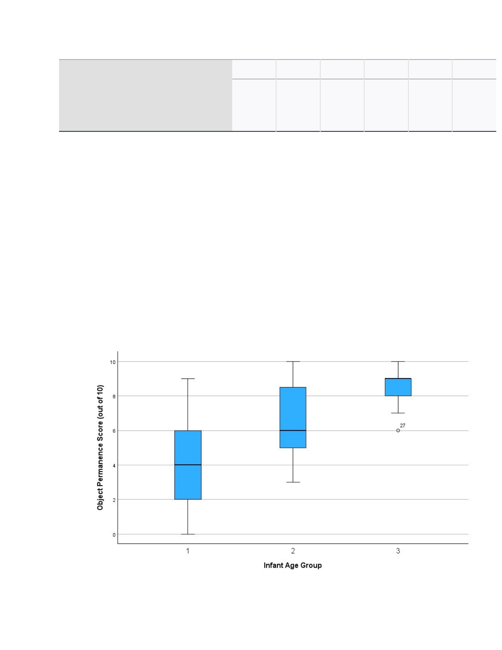
A one-way ANOVA test was conducted, and also an analysis of variance was also done to
see if there are any possible effects of different age groups on the scores that were
obtained in an assessment task. The independent variable was the age group, and there
were three different age groups, which were 9 months, 12 months, and 15 months. The
dependent variable was the score within the age groups, and these scores represented
the performance scores on the tasks and assessments. The description of the statistics
showed that there is a noticeable increase in the mean scores as the age increases and
progresses. The 9-month group had results of M=4.20, and SD=2.90, and this showed
lower scores of the ones who were 12 months. The 12-month results were M=6.50,
SD=2.45and the 15month group results were M=8.50, SD=1.27. This group showed the
highest scores out of all the groups. The overall results show that age hugely has a huge
influence on the performance on the developmental tasks and tests, and age also shows
a big influence because the older age group had higher scores than the younger age
group.
Problem Set 3: Cumulative Knowledge Question
Research Scenario: Research Scenario: A sports psychologist is studying the efficacy of a new
public school health program on the number of minutes 10th graders exercise per week. She
surveys a sample of eight 10th graders before the program begins and records the number of
minutes they report exercising per week. After two months in the program, the students are
surveyed again. The data are listed in the table below.
Using this table, enter the data into a new SPSS data file. Choose and run the correct analysis
(it will be one learned in a previous module) to determine whether the new public health
program significantly increases the number of minutes exercised for 10th graders. Remember
to put your initials within any and all variable names. Choose and create the correct graph
that corresponds with this analysis. Follow the directions below the table to complete this
part.
Minutes Ex./Wk.
Before Program
Minutes Ex./Wk.
After Program
45
45
90
55
100
50
45
120
70
120
160
30
60
170
20
70
1. Paste SPSS output. (10 pts)
Paired Samples Statistics
Paired Samples Correlations
N
Corre
lation
Signifi
OneSided
p
cance
Two-
Sided p
Mean N
Std.
Deviation
Std. Error
Mean
Pair 1 Mintues Exercised per
Week Before Program
73.13 8 42.252 14.938
Mintues Exercised per
Week After Program
83.13 8 49.493 17.498
P
a
i
r
1
Mintues Exercised
per Week Before
Program & Mintues
Exercised per Week
After Program
8 .977 <.001 <.001
Paired Samples Effect Sizes
Sta
nda
rdiz
era
P
o
i
n
t
E
s
t
i
m
a
t
e
95%
Confid
ence
Interval
L
o
w
e
r
Up
p
e
P
a
i
r
1
Mi
nt
ue
s
Ex
erc
ise
d
pe
r
W
ee
Cohe
n's d
12.
24
7
-
.
8
1
6
-1.6
0
6
.01
4
Hedg
es'
corre
ction
13.
78
9
-
.
7
2
5
-1.4
2
6
.01
3

k
Be
for
e
Pr
og
ra
m
-
Mi
nt
ue
s
Exercis
ed per
Week
After
Progra
m
a. The denominator used in estimating the effect sizes.
Cohen's d uses the sample standard deviation of the mean difference.
Hedges' correction uses the sample standard deviation of the mean difference, plus a
correction factor.
2. Write an APA-style Results section based on your analysis. Include your graph as an APA-
style Figure, with figure number and title, as demonstrated in the Results Section
presentation. (Results = 12 pts; Figure = 8 pts)
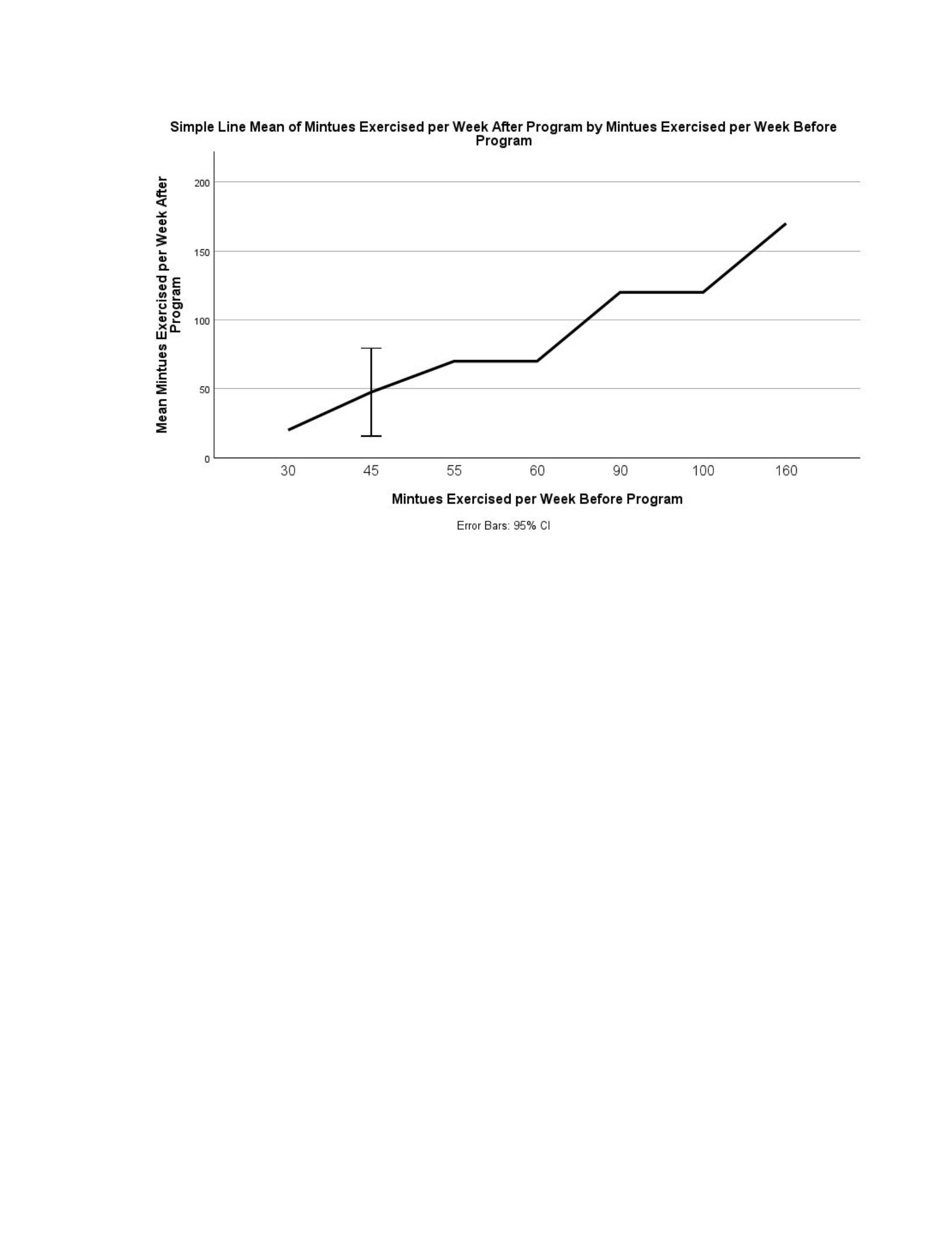
Paired-samples t-tests were done to see if there were any differences in the time between
the group before and the group after. The description of the statistics for the paired samples
can be found in the graph below. There is a high and positive correlation, which was r=.977
and p=<.001, and this was found between the group minutes before and the group minutes
after, which shows a strong relationship between the two groups and variables. The paired

samples t-test has shown a huge decrease in the minutes before to the minted after the
intervention that was conducted during the tests and analysis. After the intervention, it
showed that t(7)=-2.309 and p=.27. The overall mean difference was about -10 minutes. This
can show that the participants or the mean people spent around 10 minutes less after the
intervention that was conducted in the study. In the end, the results and findings show a big
reduction in the time that was spent before and after the intervention. This shows the
effects of the decrease in the duration of the activity.