


MATH 332 - Multivariable Calculus Question
Bank
Question 1
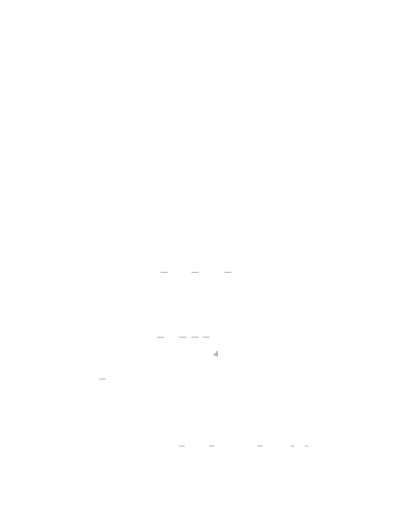
Problem Statement: Given the vector field F = (y, x, z2)andthecurveCdefinedbytheparametricequationsx =
t, y =t2, andz =t3fortfrom0to1, evaluatethelineintegralof F alongC.
Solution:
Step 1: Parametrize the curve C. The curve C is already given in parametric
form:
x=t, y =t2, z =t3
where t ranges from 0 to 1.
Step 2: Differentiate the parametric equations. Differentiate each component
with respect to t: dx
dt = 1,dy
dt = 2t, dz
dt = 3t2
Step 3: Substitute into the vector field F. Substitute x, y, and z into the
vector field F:
F(x(t), y(t), z(t)) = (y, x, z2)=(t2, t, t6)
Step 4: Find the differential of r(t). Determine dr/dt by combining the
differential components:
dr
dt =dx
dt ,dy
dt ,dz
dt = (1,2t, 3t2)
Step 5: Compute the dot product F
dr/dt. Calculate the dot product of
F and dr/dt:
F·dr
dt = (t2, t, t6)·(1,2t, 3t2) = t2·1 + t·2t+t6·3t2=t2+ 2t2+ 3t8= 3t2+ 3t8
Step 6: Set up the integral. Integrate the result of the dot product from t
= 0 to t = 1:
Z1
0
(3t2+ 3t8)dt
Step 7: Evaluate the integral. Compute the integral:
Z1
0
3t2dt +Z1
0
3t8dt = 3 t3
31
0
+ 3 t9
91
0
=t31
0+t9
31
0
= 1 + 1
3=4
3
1
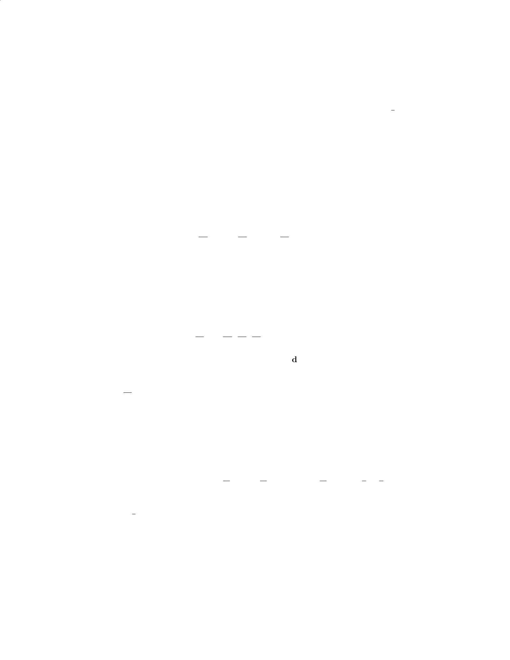
Conclusion: The line integral of the vector field F along the curve C is 4
3.
Question 1: Evaluating a Line Integral Along a Vector Field
Problem Statement: Given the vector field F = (y, x, z2)andthecurveCdefinedbytheparametricequationsx =
t, y =t2, andz =t3fortfrom0to1, evaluatethelineintegralof F alongC.
Solution:
Step 1: Parametrize the curve C. The curve C is already given in
parametric form:
x=t, y =t2, z =t3
where t ranges from 0 to 1.
Step 2: Differentiate the parametric equations. Differentiate each
component with respect to t:
dx
dt = 1,dy
dt = 2t, dz
dt = 3t2
Step 3: Substitute into the vector field F. Substitute x, y, and z
into the vector field F:
F(x(t), y(t), z(t)) = (y, x, z2)=(t2, t, t6)
Step 4: Find the differential of r(t). Determine dr/dt by combining
the differential components:
dr
dt =dx
dt ,dy
dt ,dz
dt = (1,2t, 3t2)
Step 5: Compute the dot product F
dr/dt. Calculate the dot
product of F and dr/dt:
F·dr
dt = (t2, t, t6)·(1,2t, 3t2) = t2·1 + t·2t+t6·3t2=t2+ 2t2+ 3t8= 3t2+ 3t8
Step 6: Set up the integral. Integrate the result of the dot product
from t = 0 to t = 1:
Z1
0
(3t2+ 3t8)dt
Step 7: Evaluate the integral. Compute the integral:
Z1
0
3t2dt +Z1
0
3t8dt = 3 t3
31
0
+ 3 t9
91
0
=t31
0+t9
31
0
= 1 + 1
3=4
3
Conclusion: The line integral of the vector field F along the curve
C is 4
3.
2
Question 2
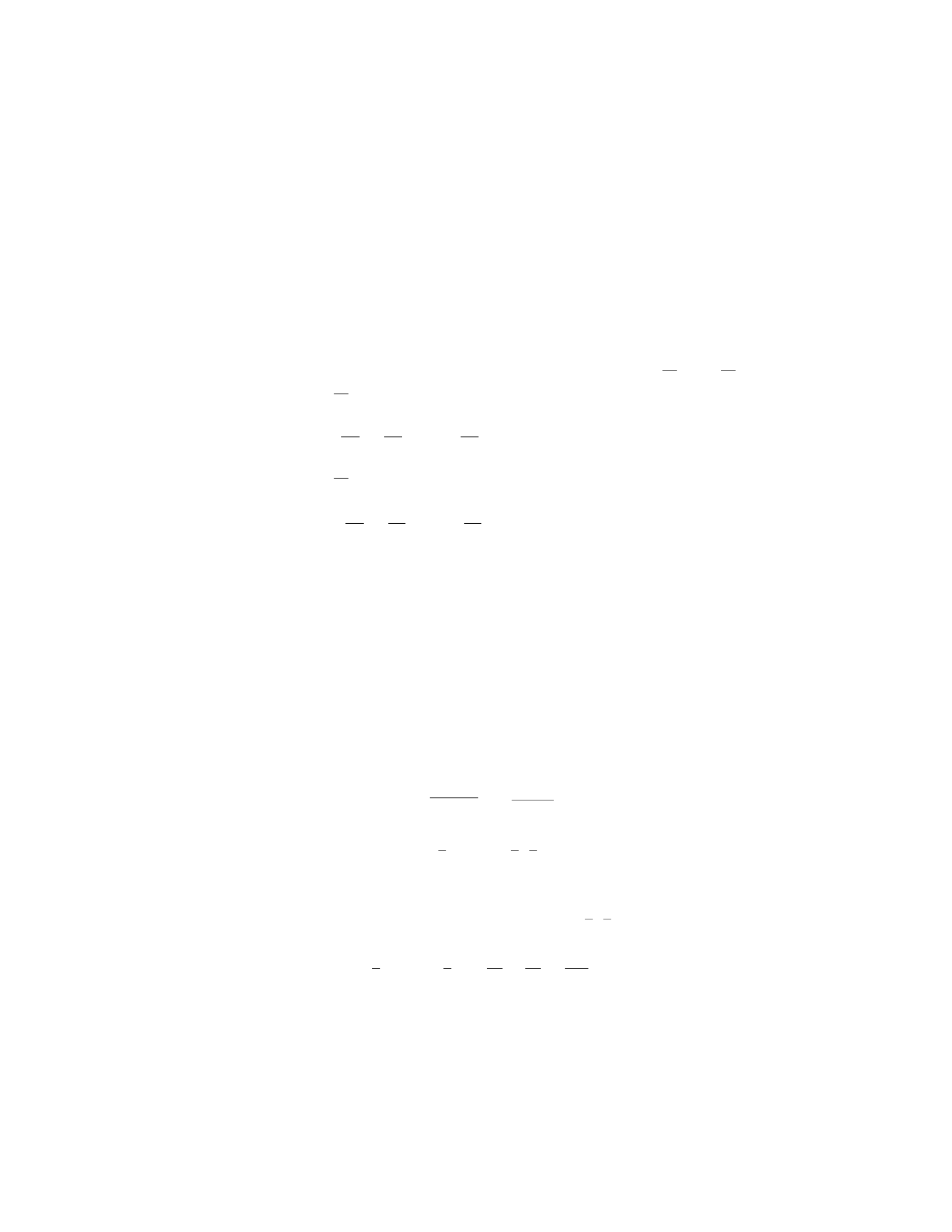
Problem: Consider the function f(x, y) = x2y+ 3xy2. Calculate:
1. The gradient of the function f. 2. The directional derivative of
fat the point (1,2) in the direction of the vector v =⟨3,4⟩.
—
Solution:
Part 1: Gradient of the function
The gradient of a function f(x, y)is a vector of partial derivatives
of f. For the function f(x, y) = x2y+ 3xy2, we need to find ∂f
∂x and ∂f
∂y .
1. Calculate ∂f
∂x :
∂f
∂x =∂
∂x (x2y) + ∂
∂x (3xy2) = 2xy + 3y2
2. Calculate ∂f
∂y :
∂f
∂y =∂
∂y (x2y) + ∂
∂y (3xy2) = x2+ 6xy
Thus, the gradient vector ∇fis:
∇f=⟨2xy + 3y2, x2+ 6xy⟩
Part 2: Directional derivative at (1,2) in the direction of v =⟨3,4⟩
The directional derivative of fat a point (x0, y0)in the direction
of the unit vector u is given by ∇f(x0, y0)·u. First, calculate ∇fat
(1,2):
1. Substitute x= 1 and y= 2 into ∇f:
∇f(1,2) = ⟨2(1)(2) + 3(2)2,12+ 6(1)(2)⟩=⟨4 + 12,1 + 12⟩=⟨16,13⟩
2. Normalize the direction vector v =⟨3,4⟩:
∥v∥=p32+ 42=√9 + 16 = 5
u=1
5⟨3,4⟩=⟨3
5,4
5⟩
3. Calculate the directional derivative:
Duf(1,2) = ∇f(1,2) ·u=⟨16,13⟩·⟨3
5,4
5⟩
= 16 3
5+ 13 4
5=48
5+52
5=100
5= 20
Thus, the directional derivative of fat the point (1,2) in the di-
rection of v =⟨3,4⟩is 20. Question 2: Finding the Gradient and
Directional Derivative
3

Problem: Consider the function f(x, y) = x2y+ 3xy2. Calculate:
1. The gradient of the function f. 2. The directional derivative of
fat the point (1,2) in the direction of the vector v =⟨3,4⟩.
—
Solution:
Part 1: Gradient of the function
The gradient of a function f(x, y)is a vector of partial derivatives
of f. For the function f(x, y) = x2y+ 3xy2, we need to find ∂f
∂x and ∂f
∂y .
1. Calculate ∂f
∂x :
∂f
∂x =∂
∂x (x2y) + ∂
∂x (3xy2) = 2xy + 3y2
2. Calculate ∂f
∂y :
∂f
∂y =∂
∂y (x2y) + ∂
∂y (3xy2) = x2+ 6xy
Thus, the gradient vector ∇fis:
∇f=⟨2xy + 3y2, x2+ 6xy⟩
Part 2: Directional derivative at (1,2) in the direction of v =⟨3,4⟩
The directional derivative of fat a point (x0, y0)in the direction
of the unit vector u is given by ∇f(x0, y0)·u. First, calculate ∇fat
(1,2):
1. Substitute x= 1 and y= 2 into ∇f:
∇f(1,2) = ⟨2(1)(2) + 3(2)2,12+ 6(1)(2)⟩=⟨4 + 12,1 + 12⟩=⟨16,13⟩
2. Normalize the direction vector v =⟨3,4⟩:
∥v∥=p32+ 42=√9 + 16 = 5
u=1
5⟨3,4⟩=⟨3
5,4
5⟩
3. Calculate the directional derivative:
Duf(1,2) = ∇f(1,2) ·u=⟨16,13⟩·⟨3
5,4
5⟩
= 16 3
5+ 13 4
5=48
5+52
5=100
5= 20
Thus, the directional derivative of fat the point (1,2) in the di-
rection of v =⟨3,4⟩is 20.
4
Question 3
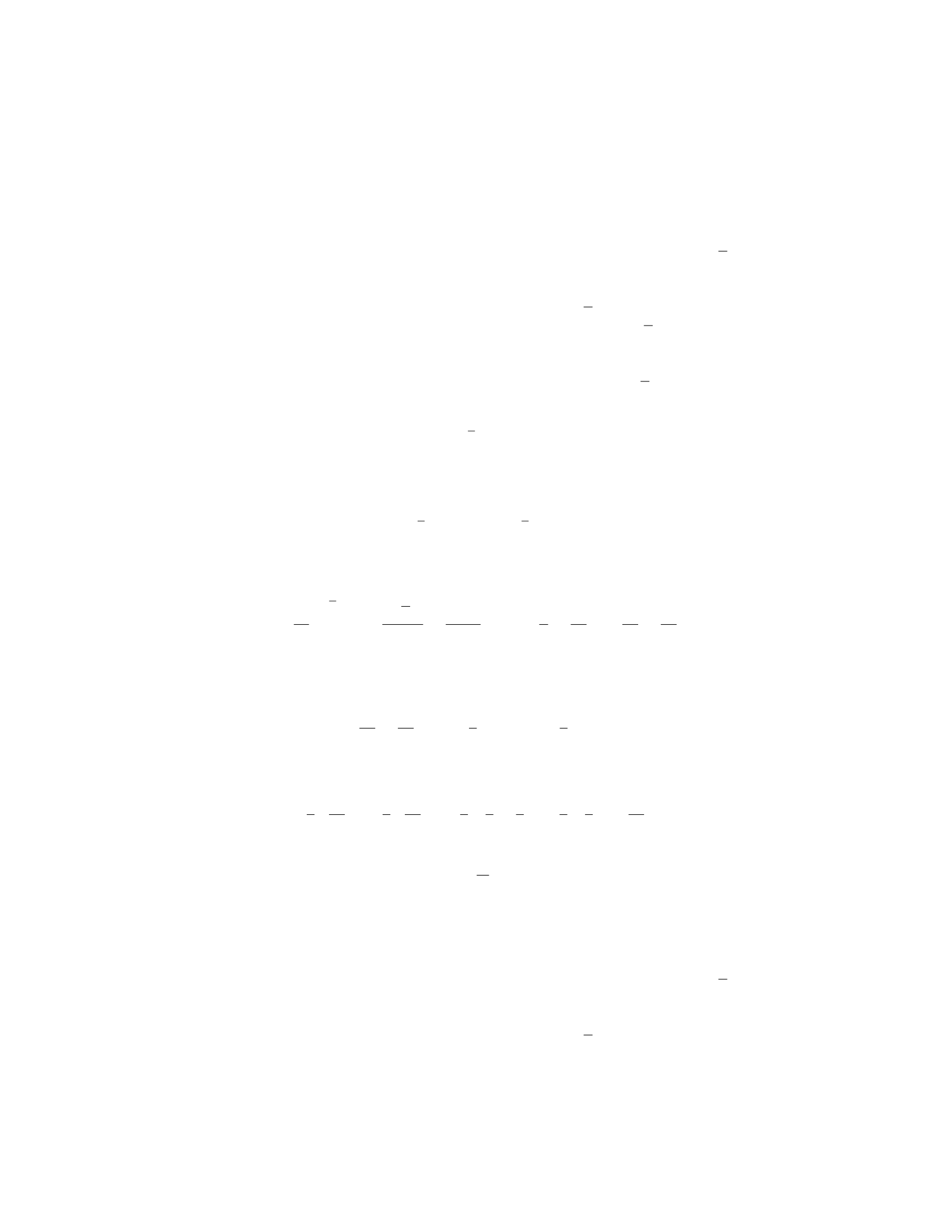
Problem Statement: Evaluate the double integral R RRxy dA where
Ris the region in the first quadrant bounded by y=x2and y=√x.
Solution:
Step 1: Sketch the Region To better understand the limits of
integration, sketch the curves y=x2and y=√x. Both curves pass
through (0,0) and (1,1) with y=x2lying below y=√xwithin the
region of interest.
Step 2: Set Up the Double Integral The curves intersect at x= 0
and x= 1. For each xin this range, yvaries from x2to √x. Therefore,
the double integral is set up as follows:
Z1
0Z√x
x2
xy dy dx
Step 3: Integrate with Respect to y: Fix xand integrate with
respect to y:
Z√x
x2
xy dy =xZ√x
x2
y dy
This integral computes as:
xy2
2√x
x2
=x(√x)2
2−(x2)2
2=xx
2−x4
2=x2
2−x5
2
Step 4: Integrate with Respect to x: Now integrate the result from
the previous step over x:
Z1
0x2
2−x5
2dx =1
2Z1
0
x2dx −1
2Z1
0
x5dx
Each of these integrals can be computed using the power rule:
1
2x3
31
0−1
2x6
61
0
=1
21
3−1
6=1
21
6=1
12
Step 5: Final Answer Therefore, the value of the double integral
R RRxy dA over the given region is 1
12 .
This problem showcases how to set limits for a double integral over
a non-rectangular region and evaluate it by integrating in stages, first
with respect to one variable, then the other. Question 3: Evaluating
a Double Integral Over a General Region
Problem Statement: Evaluate the double integral R RRxy dA where
Ris the region in the first quadrant bounded by y=x2and y=√x.
Solution:
Step 1: Sketch the Region To better understand the limits of
integration, sketch the curves y=x2and y=√x. Both curves pass
5
through (0,0) and (1,1) with y=x2lying below y=√xwithin the
region of interest.
Step 2: Set Up the Double Integral The curves intersect at x= 0
and x= 1. For each xin this range, yvaries from x2to √x. Therefore,
the double integral is set up as follows:
Z1
0Z√x
x2
xy dy dx
Step 3: Integrate with Respect to y: Fix xand integrate with
respect to y:
Z√x
x2
xy dy =xZ√x
x2
y dy
This integral computes as:
xy2
2√x
x2
=x(√x)2
2−(x2)2
2=xx
2−x4
2=x2
2−x5
2
Step 4: Integrate with Respect to x: Now integrate the result from
the previous step over x:
Z1
0x2
2−x5
2dx =1
2Z1
0
x2dx −1
2Z1
0
x5dx
Each of these integrals can be computed using the power rule:
1
2x3
31
0−1
2x6
61
0
=1
21
3−1
6=1
21
6=1
12
Step 5: Final Answer Therefore, the value of the double integral
R RRxy dA over the given region is 1
12 .
This problem showcases how to set limits for a double integral over
a non-rectangular region and evaluate it by integrating in stages, first
with respect to one variable, then the other.
Question 4
Problem Statement: Consider the function f(x, y, z) = x2y+eyz +
zcos(x). Find the gradient of fat the point (1, 0, π) and then compute
the directional derivative of fat this point in the direction of the
vector v = (2,−2,1).
Solution:
Step 1: Find partial derivatives of f.
The function given is f(x, y, z) = x2y+eyz +zcos(x).
- Partial Derivative with respect to x:
∂f
∂x = 2xy −zsin(x)
6

- Partial Derivative with respect to y:
∂f
∂y =x2+zeyz
- Partial Derivative with respect to z:
∂f
∂z =eyzy+ cos(x)
Step 2: Evaluate the partial derivatives at the point (1, 0, π).
- At (1, 0, π):
∂f
∂x (1,0, π) = 2(1)(0) −πsin(1) = −πsin(1)
∂f
∂y (1,0, π)=12+πe(0)(π)= 1 + π
∂f
∂z (1,0, π) = e(0)(π)0 + cos(1) = cos(1)
Step 3: Construct the gradient vector at (1, 0, π).
∇f(1,0, π)=(−πsin(1),1 + π, cos(1))
Step 4: Normalize the direction vector v = (2,−2,1).
Calculate the magnitude of v:
∥v∥=p22+ (−2)2+ 12=√4 + 4 + 1 = √9 = 3
Normalized vector u is:
u=2
3,−2
3,1
3
Step 5: Compute the directional derivative in direction of v.
Using the formula for the directional derivative along u:
Duf(1,0, π) = ∇f(1,0, π)·u= (−πsin(1),1 + π, cos(1)) ·2
3,−2
3,1
3
= (−πsin(1)) 2
3+ (1 + π)−2
3+ cos(1) 1
3
=−2πsin(1)
3−2(1 + π)
3+cos(1)
3
Answer: The gradient of fat (1, 0, π) is (−πsin(1),1 + π, cos(1))
and the directional derivative of fin the direction of v is −2πsin(1)
3−
2(1+π)
3+cos(1)
3. Question 4: Gradient and Directional Derivative
7

Problem Statement: Consider the function f(x, y, z) = x2y+eyz +
zcos(x). Find the gradient of fat the point (1, 0, π) and then compute
the directional derivative of fat this point in the direction of the
vector v = (2,−2,1).
Solution:
Step 1: Find partial derivatives of f.
The function given is f(x, y, z) = x2y+eyz +zcos(x).
- Partial Derivative with respect to x:
∂f
∂x = 2xy −zsin(x)
- Partial Derivative with respect to y:
∂f
∂y =x2+zeyz
- Partial Derivative with respect to z:
∂f
∂z =eyzy+ cos(x)
Step 2: Evaluate the partial derivatives at the point (1, 0, π).
- At (1, 0, π):
∂f
∂x (1,0, π) = 2(1)(0) −πsin(1) = −πsin(1)
∂f
∂y (1,0, π)=12+πe(0)(π)= 1 + π
∂f
∂z (1,0, π) = e(0)(π)0 + cos(1) = cos(1)
Step 3: Construct the gradient vector at (1, 0, π).
∇f(1,0, π)=(−πsin(1),1 + π, cos(1))
Step 4: Normalize the direction vector v = (2,−2,1).
Calculate the magnitude of v:
∥v∥=p22+ (−2)2+ 12=√4 + 4 + 1 = √9 = 3
Normalized vector u is:
u=2
3,−2
3,1
3
Step 5: Compute the directional derivative in direction of v.
Using the formula for the directional derivative along u:
Duf(1,0, π) = ∇f(1,0, π)·u= (−πsin(1),1 + π, cos(1)) ·2
3,−2
3,1
3
8
= (−πsin(1)) 2
3+ (1 + π)−2
3+ cos(1) 1
3
=−2πsin(1)
3−2(1 + π)
3+cos(1)
3
Answer: The gradient of fat (1, 0, π) is (−πsin(1),1 + π, cos(1))
and the directional derivative of fin the direction of v is −2πsin(1)
3−
2(1+π)
3+cos(1)
3.
Question 5
Problem Statement: Evaluate the double integral of the function
f(x, y) = x2y+2yover the rectangular region bounded by x= 0 to x= 2
and y=−1to y= 1.
Solution
Step 1: Set up the double integral. Since the region of integration
is rectangular, we set up the integral as follows:
Z2
x=0 Z1
y=−1
(x2y+ 2y)dy dx
Step 2: Integrate with respect to yfirst. Begin by computing the
inner integral:
Z1
y=−1
(x2y+ 2y)dy
x2Z1
y=−1
y dy + 2 Z1
y=−1
y dy
Note that both Ry dy from −1to 1result in zero because the func-
tion yis odd and the limits of integration are symmetric about the
origin. Therefore:
x2·0+2·0=0
Step 3: Integrate the result with respect to x. The result of the
integral from Step 2 is zero, hence:
Z2
x=0
0dx = 0
Conclusion: The value of the double integral R2
x=0 R1
y=−1(x2y+2y)dy dx
is 0.
Final Answer The double integral evaluates to 0. Question 5: Eval-
uating a Double Integral Over a Rectangular Region
Problem Statement: Evaluate the double integral of the function
f(x, y) = x2y+2yover the rectangular region bounded by x= 0 to x= 2
and y=−1to y= 1.
9

Solution
Step 1: Set up the double integral. Since the region of integration
is rectangular, we set up the integral as follows:
Z2
x=0 Z1
y=−1
(x2y+ 2y)dy dx
Step 2: Integrate with respect to yfirst. Begin by computing the
inner integral:
Z1
y=−1
(x2y+ 2y)dy
x2Z1
y=−1
y dy + 2 Z1
y=−1
y dy
Note that both Ry dy from −1to 1result in zero because the func-
tion yis odd and the limits of integration are symmetric about the
origin. Therefore:
x2·0+2·0=0
Step 3: Integrate the result with respect to x. The result of the
integral from Step 2 is zero, hence:
Z2
x=0
0dx = 0
Conclusion: The value of the double integral R2
x=0 R1
y=−1(x2y+2y)dy dx
is 0.
Final Answer The double integral evaluates to 0.
Question 6
Problem Statement: A hill is modeled by the height function z=
f(x, y) = 1.5x2+xy +y2. A hiker is standing at the point (2,1) on this
hill.
a) Calculate the gradient vector ∇fat the point (2,1).
b) Determine the direction of the steepest ascent from the point
(2,1).
c) Calculate the directional derivative of fat (2,1) in the direction
of the vector v =⟨3,−4⟩.
Solution:
a) Calculating the Gradient Vector ∇fat (2,1)
Step 1: Find the partial derivatives of f(x, y). - ∂f
∂x = 3x+y-
∂f
∂y =x+ 2y
Step 2: Evaluate the partial derivatives at the point (2,1). -
∂f
∂x (2,1) = 3(2) + 1 = 7 -∂f
∂y (2,1) = 2 + 2(1) = 4
10

Step 3: Write the gradient vector. - ∇f(2,1) = ⟨7,4⟩
b) Direction of the Steepest Ascent
The gradient vector ∇fpoints in the direction of the steepest
ascent. - From the previous part, ∇f(2,1) = ⟨7,4⟩is the direction of
the steepest ascent.
c) Calculating the Directional Derivative in the direction of v =
⟨3,−4⟩
Step 1: Normalize the vector v. - Magnitude of v is ∥v∥=p32+ (−4)2=
√9 + 16 = 5. - Unit vector u is ⟨3
5,−4
5⟩.
Step 2: The directional derivative Dufat (2,1) is given by ∇f·u.
- Plug in ∇f(2,1) and u:
∇f(2,1) ·u=⟨7,4⟩·⟨3
5,−4
5⟩= 7 3
5+ 4 −4
5
=21
5−16
5=5
5= 1
Final Answers: - a) ∇f(2,1) = ⟨7,4⟩- b) Direction of steepest as-
cent: ⟨7,4⟩- c) Directional derivative in direction ⟨3,−4⟩is 1. Question
6: Multivariable Calculus - Gradient Vector and Directional Deriva-
tive
Problem Statement: A hill is modeled by the height function z=
f(x, y) = 1.5x2+xy +y2. A hiker is standing at the point (2,1) on this
hill.
a) Calculate the gradient vector ∇fat the point (2,1).
b) Determine the direction of the steepest ascent from the point
(2,1).
c) Calculate the directional derivative of fat (2,1) in the direction
of the vector v =⟨3,−4⟩.
Solution:
a) Calculating the Gradient Vector ∇fat (2,1)
Step 1: Find the partial derivatives of f(x, y). - ∂f
∂x = 3x+y-
∂f
∂y =x+ 2y
Step 2: Evaluate the partial derivatives at the point (2,1). -
∂f
∂x (2,1) = 3(2) + 1 = 7 -∂f
∂y (2,1) = 2 + 2(1) = 4
Step 3: Write the gradient vector. - ∇f(2,1) = ⟨7,4⟩
b) Direction of the Steepest Ascent
The gradient vector ∇fpoints in the direction of the steepest
ascent. - From the previous part, ∇f(2,1) = ⟨7,4⟩is the direction of
the steepest ascent.
c) Calculating the Directional Derivative in the direction of v =
⟨3,−4⟩
Step 1: Normalize the vector v. - Magnitude of v is ∥v∥=p32+ (−4)2=
√9 + 16 = 5. - Unit vector u is ⟨3
5,−4
5⟩.
11

Step 2: The directional derivative Dufat (2,1) is given by ∇f·u.
- Plug in ∇f(2,1) and u:
∇f(2,1) ·u=⟨7,4⟩·⟨3
5,−4
5⟩= 7 3
5+ 4 −4
5
=21
5−16
5=5
5= 1
Final Answers: - a) ∇f(2,1) = ⟨7,4⟩- b) Direction of steepest as-
cent: ⟨7,4⟩- c) Directional derivative in direction ⟨3,−4⟩is 1.
Question 7
Problem:
Evaluate the limit of the function f(x, y) = xy
x2+y2as (x, y)approaches
(0,0).
Questions:
1. What does it mean to find the limit of a function as (x, y)
approaches a point in multivariable calculus? 2. How might one
approach finding the limit of f(x, y) = xy
x2+y2as (x, y)→(0,0)? 3. Why
is it useful to convert to polar coordinates when evaluating the limit of
f(x, y)as (x, y)approaches (0,0)? 4. Calculate lim(x,y)→(0,0) xy
x2+y2using
polar coordinates. 5. How do the results from different approaches
help to determine whether the original limit exists?
Solutions:
Step 1: Understanding the Limit in Multivariable Calculus
- Answer: In multivariable calculus, finding the limit of a function
as (x, y)approaches a particular point (say, (a, b)) means determining
what value the function approaches as the point (x, y)gets arbitrarily
close to (a, b)from any path in the xy-plane.
Step 2: Approaching the Limit Evaluation
- Answer: To find the limit of f(x, y) = xy
x2+y2as (x, y)→(0,0), we
should initially consider approaching (0,0) along various paths like
y=mx (where mis a constant), y=x2, etc., and see if the limits are
consistent.
Step 3: Reason for Using Polar Coordinates
- Answer: Polar coordinates are useful because they can simplify
the algebra and offer a uniform approach to assessing the behavior of
f(x, y)as r(the distance from the origin) approaches 0. This provides
a holistic view by considering all paths simultaneously as r→0, where
rand θdescribe any point in the plane.
Step 4: Calculation Using Polar Coordinates
- Step-by-step calculation:
12

1. Convert to polar coordinates: Express xand yin terms of rand
θ:x=rcos θand y=rsin θ. Therefore,
f(x, y) = rcos θ·rsin θ
(rcos θ)2+ (rsin θ)2=r2cos θsin θ
r2(cos2θ+ sin2θ)=cos θsin θ
1.
2. Simplify: Notice that cos2θ+ sin2θ= 1, so
f(x, y) = cos θsin θ.
3. Evaluate the limit: As r→0,
lim
(x,y)→(0,0) f(x, y) = lim
r→0cos θsin θ.
This does not depend on r, but since cos θsin θis bounded between
−1/2and 1/2, the function does not approach a single value as r→0.
Step 5: Interpreting Results
- Answer: Since the limit of cos θsin θdepends on θand does not
converge to a single value as (x, y)→(0,0), the original limit does
not exist. This is confirmed by the fact that approaching (0,0) along
different paths (e.g., along y=xvs. y= 0) gives different limits,
indicating the non-existence of the limit. Question 7: Multivariable
Calculus - Finding Limits of a Multivariable Function
Problem:
Evaluate the limit of the function f(x, y) = xy
x2+y2as (x, y)approaches
(0,0).
Questions:
1. What does it mean to find the limit of a function as (x, y)
approaches a point in multivariable calculus? 2. How might one
approach finding the limit of f(x, y) = xy
x2+y2as (x, y)→(0,0)? 3. Why
is it useful to convert to polar coordinates when evaluating the limit of
f(x, y)as (x, y)approaches (0,0)? 4. Calculate lim(x,y)→(0,0) xy
x2+y2using
polar coordinates. 5. How do the results from different approaches
help to determine whether the original limit exists?
Solutions:
Step 1: Understanding the Limit in Multivariable Calculus
- Answer: In multivariable calculus, finding the limit of a function
as (x, y)approaches a particular point (say, (a, b)) means determining
what value the function approaches as the point (x, y)gets arbitrarily
close to (a, b)from any path in the xy-plane.
Step 2: Approaching the Limit Evaluation
- Answer: To find the limit of f(x, y) = xy
x2+y2as (x, y)→(0,0), we
should initially consider approaching (0,0) along various paths like
y=mx (where mis a constant), y=x2, etc., and see if the limits are
consistent.
Step 3: Reason for Using Polar Coordinates
13

- Answer: Polar coordinates are useful because they can simplify
the algebra and offer a uniform approach to assessing the behavior of
f(x, y)as r(the distance from the origin) approaches 0. This provides
a holistic view by considering all paths simultaneously as r→0, where
rand θdescribe any point in the plane.
Step 4: Calculation Using Polar Coordinates
- Step-by-step calculation:
1. Convert to polar coordinates: Express xand yin terms of rand
θ:x=rcos θand y=rsin θ. Therefore,
f(x, y) = rcos θ·rsin θ
(rcos θ)2+ (rsin θ)2=r2cos θsin θ
r2(cos2θ+ sin2θ)=cos θsin θ
1.
2. Simplify: Notice that cos2θ+ sin2θ= 1, so
f(x, y) = cos θsin θ.
3. Evaluate the limit: As r→0,
lim
(x,y)→(0,0) f(x, y) = lim
r→0cos θsin θ.
This does not depend on r, but since cos θsin θis bounded between
−1/2and 1/2, the function does not approach a single value as r→0.
Step 5: Interpreting Results
- Answer: Since the limit of cos θsin θdepends on θand does not
converge to a single value as (x, y)→(0,0), the original limit does
not exist. This is confirmed by the fact that approaching (0,0) along
different paths (e.g., along y=xvs. y= 0) gives different limits,
indicating the non-existence of the limit.
Question 8
Problem Statement: Calculate the surface integral of the vector
field F = (x2, yz, z2)over the surface Swhich is the paraboloid z=
1−x2−y2for z≥0, with upward orientation.
Step-by-Step Solution:
Step 1: Parametrize the SurfaceSThe surface is a paraboloid, and
can be parametrized using polar coordinates:
r(r, θ)=(rcos θ, r sin θ, 1−r2)
where 0≤r≤1and 0≤θ≤2π.
Step 2: Calculate rrand rθCompute the partial derivatives of r
with respect to rand θ:
rr= (cos θ, sin θ, −2r)
14

rθ= (−rsin θ, r cos θ, 0)
Step 3: Calculate the Normal Vector n Using the Cross Product
Find the cross product of rrand rθ:
n=rr×rθ=
i j k
cos θsin θ−2r
−rsin θ r cos θ0
n= (2r2cos θ, 2r2sin θ, r)
Step 4: Modify n for Correct Orientation Since the orientation of
the surface is upward, ensure the z-component of n is positive:
n= (−2r2cos θ, −2r2sin θ, r)
Step 5: Evaluate the Vector Field F at Surface Points Substitute
the parametrization into F:
F(r(r, θ)) = (r2cos2θ, r sin θ(1 −r2),(1 −r2)2)
Step 6: Compute F ·n Find the dot product of F and n:
F·n= (r2cos2θ)(−2r2cos θ)+(rsin θ(1 −r2))(−2r2sin θ) + ((1 −r2)2)(r)
F·n=−2r4cos3θ−2r3sin2θ(1 −r2) + r(1 −r2)2
Step 7: Set Up the Surface Integral
ZS
F·dS=Z2π
0Z1
0
(−2r4cos3θ−2r3sin2θ(1 −r2) + r(1 −r2)2)r dr dθ
Step 8: Integrate This involves integrating with respect to rthen
θ. Some terms (in cos3θand sin2θcos3θ) integrate to zero over the
interval 0to 2π. Thus evaluate the remaining terms.
Step 9: Evaluate Result Complete the integral to find the final
result.
This problem introduces surface integrals over a parametric sur-
face using vector fields and demonstrates using polar coordinates to
simplify the geometry of the problem. Practical calculation would re-
quire executing the multiple integral in Step 8, which would typically
be performed using mathematical software or further simplifying by
hand. Question 8: Multivariable Calculus - Surface Integrals
Problem Statement: Calculate the surface integral of the vector
field F = (x2, yz, z2)over the surface Swhich is the paraboloid z=
1−x2−y2for z≥0, with upward orientation.
Step-by-Step Solution:
Step 1: Parametrize the SurfaceSThe surface is a paraboloid, and
can be parametrized using polar coordinates:
r(r, θ)=(rcos θ, r sin θ, 1−r2)
15

where 0≤r≤1and 0≤θ≤2π.
Step 2: Calculate rrand rθCompute the partial derivatives of r
with respect to rand θ:
rr= (cos θ, sin θ, −2r)
rθ= (−rsin θ, r cos θ, 0)
Step 3: Calculate the Normal Vector n Using the Cross Product
Find the cross product of rrand rθ:
n=rr×rθ=
i j k
cos θsin θ−2r
−rsin θ r cos θ0
n= (2r2cos θ, 2r2sin θ, r)
Step 4: Modify n for Correct Orientation Since the orientation of
the surface is upward, ensure the z-component of n is positive:
n= (−2r2cos θ, −2r2sin θ, r)
Step 5: Evaluate the Vector Field F at Surface Points Substitute
the parametrization into F:
F(r(r, θ)) = (r2cos2θ, r sin θ(1 −r2),(1 −r2)2)
Step 6: Compute F ·n Find the dot product of F and n:
F·n= (r2cos2θ)(−2r2cos θ)+(rsin θ(1 −r2))(−2r2sin θ) + ((1 −r2)2)(r)
F·n=−2r4cos3θ−2r3sin2θ(1 −r2) + r(1 −r2)2
Step 7: Set Up the Surface Integral
ZS
F·dS=Z2π
0Z1
0
(−2r4cos3θ−2r3sin2θ(1 −r2) + r(1 −r2)2)r dr dθ
Step 8: Integrate This involves integrating with respect to rthen
θ. Some terms (in cos3θand sin2θcos3θ) integrate to zero over the
interval 0to 2π. Thus evaluate the remaining terms.
Step 9: Evaluate Result Complete the integral to find the final
result.
This problem introduces surface integrals over a parametric sur-
face using vector fields and demonstrates using polar coordinates to
simplify the geometry of the problem. Practical calculation would re-
quire executing the multiple integral in Step 8, which would typically
be performed using mathematical software or further simplifying by
hand.
16

Question 9
Problem: Evaluate the line integral of the vector field F over the
curve C, where F = ¡2x, 3y, 4z¿, and C is the curve from (0,0,0) to
(1,1,1) parametrized by r(t) = ¡t, t, t¿ for t in [0, 1].
Solution:
Step 1: Parametrize the Curve The curve C is given by the parametriza-
tion r(t) = ¡t, t, t¿ where t varies from 0 to 1. We first compute the
derivative of r with respect to t, denoted as r’(t).
r′(t) = d
dt < t, t, t >=<1,1,1>
Step 2: Plug the Parametrization into the Vector Field We sub-
stitute the parametric form of the curve into the vector field F. Since
F = ¡2x, 3y, 4z¿, we have:
F(r(t)) = F(t, t, t) =<2t, 3t, 4t >
Step 3: Calculate the Dot Product F(r(t))
·
r’(t) We find the dot
product of F(r(t)) and r’(t):
F(r(t)) ·r′(t) =<2t, 3t, 4t > ·<1,1,1>= 2t+ 3t+ 4t= 9t
Step 4: Set Up the Integral to Evaluate the Line Integral The line
integral of F along C is given by:
ZC
F·dr=Z1
0
F(r(t)) ·r′(t)dt
ZC
F·dr=Z1
0
9t dt
Step 5: Evaluate the Integral We compute the integral:
Z1
0
9t dt = 9 t2
21
0
= 9 ·1
2= 4.5
Answer: The value of the line integral of the vector field F = ¡2x,
3y, 4z¿ over the curve C (parametrized by r(t) = ¡t, t, t¿ from t = 0
to 1) is 4.5. Question 9: Evaluating a Line Integral
Problem: Evaluate the line integral of the vector field F over the
curve C, where F = ¡2x, 3y, 4z¿, and C is the curve from (0,0,0) to
(1,1,1) parametrized by r(t) = ¡t, t, t¿ for t in [0, 1].
Solution:
Step 1: Parametrize the Curve The curve C is given by the parametriza-
tion r(t) = ¡t, t, t¿ where t varies from 0 to 1. We first compute the
derivative of r with respect to t, denoted as r’(t).
17
r′(t) = d
dt < t, t, t >=<1,1,1>
Step 2: Plug the Parametrization into the Vector Field We sub-
stitute the parametric form of the curve into the vector field F. Since
F = ¡2x, 3y, 4z¿, we have:
F(r(t)) = F(t, t, t) =<2t, 3t, 4t >
Step 3: Calculate the Dot Product F(r(t))
·
r’(t) We find the dot
product of F(r(t)) and r’(t):
F(r(t)) ·r′(t) =<2t, 3t, 4t > ·<1,1,1>= 2t+ 3t+ 4t= 9t
Step 4: Set Up the Integral to Evaluate the Line Integral The line
integral of F along C is given by:
ZC
F·dr=Z1
0
F(r(t)) ·r′(t)dt
ZC
F·dr=Z1
0
9t dt
Step 5: Evaluate the Integral We compute the integral:
Z1
0
9t dt = 9 t2
21
0
= 9 ·1
2= 4.5
Answer: The value of the line integral of the vector field F = ¡2x,
3y, 4z¿ over the curve C (parametrized by r(t) = ¡t, t, t¿ from t = 0
to 1) is 4.5.
Question 10
Problem:
Evaluate the line integral of the vector field F(x, y, z) = (2xy, x2−
yz, y2)over the curve r(t)=(t, t2, t3)from t= 0 to t= 1.
Solution:
Step 1: Parameterize the Curve
The given curve r(t)is already parameterized as:
r(t)=(t, t2, t3)
where truns from 0 to 1.
Step 2: Differentiate the Curve Parameterization
Differentiate r(t)with respect to tto find r′(t):
r′(t) = d(t)
dt ,d(t2)
dt ,d(t3)
dt = (1,2t, 3t2)
18
Step 3: Evaluate the Vector Field along the Curve
Substitute the parameterization r(t)into the vector field F(x, y, z):
F(r(t)) = (F(t, t2, t3)) = (2t·t2, t2−t3·t3,(t2)2) = (2t3, t2−t6, t4)
Step 4: Calculate F(r(t)) ·r′(t)
Compute the dot product of F(r(t)) and r′(t):
F(r(t)) ·r′(t) = (2t3, t2−t6, t4)·(1,2t, 3t2) = 2t3·1+(t2−t6)·2t+t4·3t2
= 2t3+ 2t3−2t7+ 3t6
= 4t3+ 3t6−2t7
Step 5: Integrate over the Interval
The line integral over the curve from t= 0 to t= 1 is given by the
integral of the dot product calculated in the previous step over the
interval:
Z1
0
(4t3+ 3t6−2t7)dt
Compute the integral term by term:
Z1
0
4t3dt = 4 t4
41
0
= 1
Z1
0
3t6dt = 3 t7
71
0
=3
7
Z1
0
2t7dt = 2 t8
81
0
=1
4
Combining these, we have:
Z1
0
(4t3+ 3t6−2t7)dt = 1 + 3
7−1
4= 1 + 12
28 −7
28 =25
28
Conclusion:
The value of the line integral of the vector field F along the curve
r(t)from t= 0 to t= 1 is 25
28 . Question 10 - Path Integral in Multivari-
able Calculus
Problem:
Evaluate the line integral of the vector field F(x, y, z) = (2xy, x2−
yz, y2)over the curve r(t)=(t, t2, t3)from t= 0 to t= 1.
Solution:
Step 1: Parameterize the Curve
The given curve r(t)is already parameterized as:
r(t)=(t, t2, t3)
19
where truns from 0 to 1.
Step 2: Differentiate the Curve Parameterization
Differentiate r(t)with respect to tto find r′(t):
r′(t) = d(t)
dt ,d(t2)
dt ,d(t3)
dt = (1,2t, 3t2)
Step 3: Evaluate the Vector Field along the Curve
Substitute the parameterization r(t)into the vector field F(x, y, z):
F(r(t)) = (F(t, t2, t3)) = (2t·t2, t2−t3·t3,(t2)2) = (2t3, t2−t6, t4)
Step 4: Calculate F(r(t)) ·r′(t)
Compute the dot product of F(r(t)) and r′(t):
F(r(t)) ·r′(t) = (2t3, t2−t6, t4)·(1,2t, 3t2) = 2t3·1+(t2−t6)·2t+t4·3t2
= 2t3+ 2t3−2t7+ 3t6
= 4t3+ 3t6−2t7
Step 5: Integrate over the Interval
The line integral over the curve from t= 0 to t= 1 is given by the
integral of the dot product calculated in the previous step over the
interval:
Z1
0
(4t3+ 3t6−2t7)dt
Compute the integral term by term:
Z1
0
4t3dt = 4 t4
41
0
= 1
Z1
0
3t6dt = 3 t7
71
0
=3
7
Z1
0
2t7dt = 2 t8
81
0
=1
4
Combining these, we have:
Z1
0
(4t3+ 3t6−2t7)dt = 1 + 3
7−1
4= 1 + 12
28 −7
28 =25
28
Conclusion:
The value of the line integral of the vector field F along the curve
r(t)from t= 0 to t= 1 is 25
28 .
20
Question 2
Problem: Consider the function f(x, y) = x2y+ 3xy2. Calculate:
1. The gradient of the function f. 2. The directional derivative of
fat the point (1,2) in the direction of the vector v =⟨3,4⟩.
—
Solution:
Part 1: Gradient of the function
The gradient of a function f(x, y)is a vector of partial derivatives
of f. For the function f(x, y) = x2y+ 3xy2, we need to find ∂f
∂x and ∂f
∂y .
1. Calculate ∂f
∂x :
∂f
∂x =∂
∂x (x2y) + ∂
∂x (3xy2) = 2xy + 3y2
2. Calculate ∂f
∂y :
∂f
∂y =∂
∂y (x2y) + ∂
∂y (3xy2) = x2+ 6xy
Thus, the gradient vector ∇fis:
∇f=⟨2xy + 3y2, x2+ 6xy⟩
Part 2: Directional derivative at (1,2) in the direction of v =⟨3,4⟩
The directional derivative of fat a point (x0, y0)in the direction
of the unit vector u is given by ∇f(x0, y0)·u. First, calculate ∇fat
(1,2):
1. Substitute x= 1 and y= 2 into ∇f:
∇f(1,2) = ⟨2(1)(2) + 3(2)2,12+ 6(1)(2)⟩=⟨4 + 12,1 + 12⟩=⟨16,13⟩
2. Normalize the direction vector v =⟨3,4⟩:
∥v∥=p32+ 42=√9 + 16 = 5
u=1
5⟨3,4⟩=⟨3
5,4
5⟩
3. Calculate the directional derivative:
Duf(1,2) = ∇f(1,2) ·u=⟨16,13⟩·⟨3
5,4
5⟩
= 16 3
5+ 13 4
5=48
5+52
5=100
5= 20
Thus, the directional derivative of fat the point (1,2) in the di-
rection of v =⟨3,4⟩is 20. Question 2: Finding the Gradient and
Directional Derivative
3

Problem: Consider the function f(x, y) = x2y+ 3xy2. Calculate:
1. The gradient of the function f. 2. The directional derivative of
fat the point (1,2) in the direction of the vector v =⟨3,4⟩.
—
Solution:
Part 1: Gradient of the function
The gradient of a function f(x, y)is a vector of partial derivatives
of f. For the function f(x, y) = x2y+ 3xy2, we need to find ∂f
∂x and ∂f
∂y .
1. Calculate ∂f
∂x :
∂f
∂x =∂
∂x (x2y) + ∂
∂x (3xy2) = 2xy + 3y2
2. Calculate ∂f
∂y :
∂f
∂y =∂
∂y (x2y) + ∂
∂y (3xy2) = x2+ 6xy
Thus, the gradient vector ∇fis:
∇f=⟨2xy + 3y2, x2+ 6xy⟩
Part 2: Directional derivative at (1,2) in the direction of v =⟨3,4⟩
The directional derivative of fat a point (x0, y0)in the direction
of the unit vector u is given by ∇f(x0, y0)·u. First, calculate ∇fat
(1,2):
1. Substitute x= 1 and y= 2 into ∇f:
∇f(1,2) = ⟨2(1)(2) + 3(2)2,12+ 6(1)(2)⟩=⟨4 + 12,1 + 12⟩=⟨16,13⟩
2. Normalize the direction vector v =⟨3,4⟩:
∥v∥=p32+ 42=√9 + 16 = 5
u=1
5⟨3,4⟩=⟨3
5,4
5⟩
3. Calculate the directional derivative:
Duf(1,2) = ∇f(1,2) ·u=⟨16,13⟩·⟨3
5,4
5⟩
= 16 3
5+ 13 4
5=48
5+52
5=100
5= 20
Thus, the directional derivative of fat the point (1,2) in the di-
rection of v =⟨3,4⟩is 20.
4
Question 3
Problem Statement: Evaluate the double integral R RRxy dA where
Ris the region in the first quadrant bounded by y=x2and y=√x.
Solution:
Step 1: Sketch the Region To better understand the limits of
integration, sketch the curves y=x2and y=√x. Both curves pass
through (0,0) and (1,1) with y=x2lying below y=√xwithin the
region of interest.
Step 2: Set Up the Double Integral The curves intersect at x= 0
and x= 1. For each xin this range, yvaries from x2to √x. Therefore,
the double integral is set up as follows:
Z1
0Z√x
x2
xy dy dx
Step 3: Integrate with Respect to y: Fix xand integrate with
respect to y:
Z√x
x2
xy dy =xZ√x
x2
y dy
This integral computes as:
xy2
2√x
x2
=x(√x)2
2−(x2)2
2=xx
2−x4
2=x2
2−x5
2
Step 4: Integrate with Respect to x: Now integrate the result from
the previous step over x:
Z1
0x2
2−x5
2dx =1
2Z1
0
x2dx −1
2Z1
0
x5dx
Each of these integrals can be computed using the power rule:
1
2x3
31
0−1
2x6
61
0
=1
21
3−1
6=1
21
6=1
12
Step 5: Final Answer Therefore, the value of the double integral
R RRxy dA over the given region is 1
12 .
This problem showcases how to set limits for a double integral over
a non-rectangular region and evaluate it by integrating in stages, first
with respect to one variable, then the other. Question 3: Evaluating
a Double Integral Over a General Region
Problem Statement: Evaluate the double integral R RRxy dA where
Ris the region in the first quadrant bounded by y=x2and y=√x.
Solution:
Step 1: Sketch the Region To better understand the limits of
integration, sketch the curves y=x2and y=√x. Both curves pass
5
through (0,0) and (1,1) with y=x2lying below y=√xwithin the
region of interest.
Step 2: Set Up the Double Integral The curves intersect at x= 0
and x= 1. For each xin this range, yvaries from x2to √x. Therefore,
the double integral is set up as follows:
Z1
0Z√x
x2
xy dy dx
Step 3: Integrate with Respect to y: Fix xand integrate with
respect to y:
Z√x
x2
xy dy =xZ√x
x2
y dy
This integral computes as:
xy2
2√x
x2
=x(√x)2
2−(x2)2
2=xx
2−x4
2=x2
2−x5
2
Step 4: Integrate with Respect to x: Now integrate the result from
the previous step over x:
Z1
0x2
2−x5
2dx =1
2Z1
0
x2dx −1
2Z1
0
x5dx
Each of these integrals can be computed using the power rule:
1
2x3
31
0−1
2x6
61
0
=1
21
3−1
6=1
21
6=1
12
Step 5: Final Answer Therefore, the value of the double integral
R RRxy dA over the given region is 1
12 .
This problem showcases how to set limits for a double integral over
a non-rectangular region and evaluate it by integrating in stages, first
with respect to one variable, then the other.
Question 4
Problem Statement: Consider the function f(x, y, z) = x2y+eyz +
zcos(x). Find the gradient of fat the point (1, 0, π) and then compute
the directional derivative of fat this point in the direction of the
vector v = (2,−2,1).
Solution:
Step 1: Find partial derivatives of f.
The function given is f(x, y, z) = x2y+eyz +zcos(x).
- Partial Derivative with respect to x:
∂f
∂x = 2xy −zsin(x)
6

- Partial Derivative with respect to y:
∂f
∂y =x2+zeyz
- Partial Derivative with respect to z:
∂f
∂z =eyz y+ cos(x)
Step 2: Evaluate the partial derivatives at the point (1, 0, π).
- At (1, 0, π):
∂f
∂x (1,0, π) = 2(1)(0) −πsin(1) = −πsin(1)
∂f
∂y (1,0, π)=12+πe(0)(π)= 1 + π
∂f
∂z (1,0, π) = e(0)(π)0 + cos(1) = cos(1)
Step 3: Construct the gradient vector at (1, 0, π).
∇f(1,0, π)=(−πsin(1),1 + π, cos(1))
Step 4: Normalize the direction vector v = (2,−2,1).
Calculate the magnitude of v:
∥v∥=p22+ (−2)2+ 12=√4 + 4 + 1 = √9 = 3
Normalized vector u is:
u=2
3,−2
3,1
3
Step 5: Compute the directional derivative in direction of v.
Using the formula for the directional derivative along u:
Duf(1,0, π) = ∇f(1,0, π)·u= (−πsin(1),1 + π, cos(1)) ·2
3,−2
3,1
3
= (−πsin(1)) 2
3+ (1 + π)−2
3+ cos(1) 1
3
=−2πsin(1)
3−2(1 + π)
3+cos(1)
3
Answer: The gradient of fat (1, 0, π) is (−πsin(1),1 + π, cos(1))
and the directional derivative of fin the direction of v is −2πsin(1)
3−
2(1+π)
3+cos(1)
3. Question 4: Gradient and Directional Derivative
7

Problem Statement: Consider the function f(x, y, z) = x2y+eyz +
zcos(x). Find the gradient of fat the point (1, 0, π) and then compute
the directional derivative of fat this point in the direction of the
vector v = (2,−2,1).
Solution:
Step 1: Find partial derivatives of f.
The function given is f(x, y, z) = x2y+eyz +zcos(x).
- Partial Derivative with respect to x:
∂f
∂x = 2xy −zsin(x)
- Partial Derivative with respect to y:
∂f
∂y =x2+zeyz
- Partial Derivative with respect to z:
∂f
∂z =eyz y+ cos(x)
Step 2: Evaluate the partial derivatives at the point (1, 0, π).
- At (1, 0, π):
∂f
∂x (1,0, π) = 2(1)(0) −πsin(1) = −πsin(1)
∂f
∂y (1,0, π)=12+πe(0)(π)= 1 + π
∂f
∂z (1,0, π) = e(0)(π)0 + cos(1) = cos(1)
Step 3: Construct the gradient vector at (1, 0, π).
∇f(1,0, π)=(−πsin(1),1 + π, cos(1))
Step 4: Normalize the direction vector v = (2,−2,1).
Calculate the magnitude of v:
∥v∥=p22+ (−2)2+ 12=√4 + 4 + 1 = √9 = 3
Normalized vector u is:
u=2
3,−2
3,1
3
Step 5: Compute the directional derivative in direction of v.
Using the formula for the directional derivative along u:
Duf(1,0, π) = ∇f(1,0, π)·u= (−πsin(1),1 + π, cos(1)) ·2
3,−2
3,1
3
8
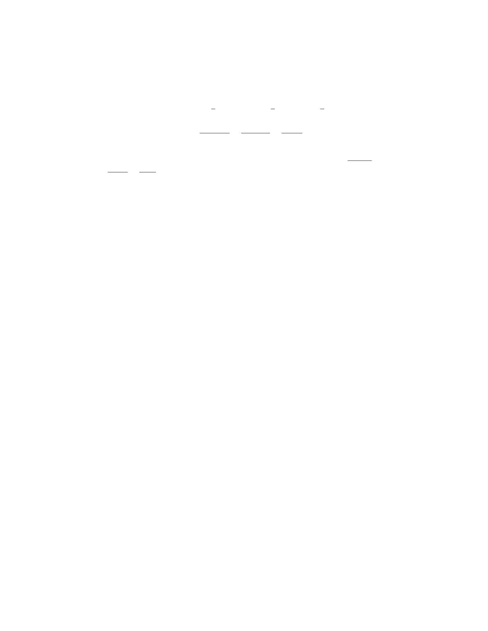
= (−πsin(1)) 2
3+ (1 + π)−2
3+ cos(1) 1
3
=−2πsin(1)
3−2(1 + π)
3+cos(1)
3
Answer: The gradient of fat (1, 0, π) is (−πsin(1),1 + π, cos(1))
and the directional derivative of fin the direction of v is −2πsin(1)
3−
2(1+π)
3+cos(1)
3.
Question 5
Problem Statement: Evaluate the double integral of the function
f(x, y) = x2y+2yover the rectangular region bounded by x= 0 to x= 2
and y=−1to y= 1.
Solution
Step 1: Set up the double integral. Since the region of integration
is rectangular, we set up the integral as follows:
Z2
x=0 Z1
y=−1
(x2y+ 2y)dy dx
Step 2: Integrate with respect to yfirst. Begin by computing the
inner integral:
Z1
y=−1
(x2y+ 2y)dy
x2Z1
y=−1
y dy + 2 Z1
y=−1
y dy
Note that both Ry dy from −1to 1result in zero because the func-
tion yis odd and the limits of integration are symmetric about the
origin. Therefore:
x2·0+2·0=0
Step 3: Integrate the result with respect to x. The result of the
integral from Step 2 is zero, hence:
Z2
x=0
0dx = 0
Conclusion: The value of the double integral R2
x=0 R1
y=−1(x2y+2y)dy dx
is 0.
Final Answer The double integral evaluates to 0. Question 5: Eval-
uating a Double Integral Over a Rectangular Region
Problem Statement: Evaluate the double integral of the function
f(x, y) = x2y+2yover the rectangular region bounded by x= 0 to x= 2
and y=−1to y= 1.
9

Solution
Step 1: Set up the double integral. Since the region of integration
is rectangular, we set up the integral as follows:
Z2
x=0 Z1
y=−1
(x2y+ 2y)dy dx
Step 2: Integrate with respect to yfirst. Begin by computing the
inner integral:
Z1
y=−1
(x2y+ 2y)dy
x2Z1
y=−1
y dy + 2 Z1
y=−1
y dy
Note that both Ry dy from −1to 1result in zero because the func-
tion yis odd and the limits of integration are symmetric about the
origin. Therefore:
x2·0+2·0=0
Step 3: Integrate the result with respect to x. The result of the
integral from Step 2 is zero, hence:
Z2
x=0
0dx = 0
Conclusion: The value of the double integral R2
x=0 R1
y=−1(x2y+2y)dy dx
is 0.
Final Answer The double integral evaluates to 0.
Question 6
Problem Statement: A hill is modeled by the height function z=
f(x, y) = 1.5x2+xy +y2. A hiker is standing at the point (2,1) on this
hill.
a) Calculate the gradient vector ∇fat the point (2,1).
b) Determine the direction of the steepest ascent from the point
(2,1).
c) Calculate the directional derivative of fat (2,1) in the direction
of the vector v =⟨3,−4⟩.
Solution:
a) Calculating the Gradient Vector ∇fat (2,1)
Step 1: Find the partial derivatives of f(x, y). - ∂f
∂x = 3x+y-
∂f
∂y =x+ 2y
Step 2: Evaluate the partial derivatives at the point (2,1). -
∂f
∂x (2,1) = 3(2) + 1 = 7 -∂f
∂y (2,1) = 2 + 2(1) = 4
10

Step 3: Write the gradient vector. - ∇f(2,1) = ⟨7,4⟩
b) Direction of the Steepest Ascent
The gradient vector ∇fpoints in the direction of the steepest
ascent. - From the previous part, ∇f(2,1) = ⟨7,4⟩is the direction of
the steepest ascent.
c) Calculating the Directional Derivative in the direction of v =
⟨3,−4⟩
Step 1: Normalize the vector v. - Magnitude of v is ∥v∥=p32+ (−4)2=
√9 + 16 = 5. - Unit vector u is ⟨3
5,−4
5⟩.
Step 2: The directional derivative Dufat (2,1) is given by ∇f·u.
- Plug in ∇f(2,1) and u:
∇f(2,1) ·u=⟨7,4⟩·⟨3
5,−4
5⟩= 7 3
5+ 4 −4
5
=21
5−16
5=5
5= 1
Final Answers: - a) ∇f(2,1) = ⟨7,4⟩- b) Direction of steepest as-
cent: ⟨7,4⟩- c) Directional derivative in direction ⟨3,−4⟩is 1. Question
6: Multivariable Calculus - Gradient Vector and Directional Deriva-
tive
Problem Statement: A hill is modeled by the height function z=
f(x, y) = 1.5x2+xy +y2. A hiker is standing at the point (2,1) on this
hill.
a) Calculate the gradient vector ∇fat the point (2,1).
b) Determine the direction of the steepest ascent from the point
(2,1).
c) Calculate the directional derivative of fat (2,1) in the direction
of the vector v =⟨3,−4⟩.
Solution:
a) Calculating the Gradient Vector ∇fat (2,1)
Step 1: Find the partial derivatives of f(x, y). - ∂f
∂x = 3x+y-
∂f
∂y =x+ 2y
Step 2: Evaluate the partial derivatives at the point (2,1). -
∂f
∂x (2,1) = 3(2) + 1 = 7 -∂f
∂y (2,1) = 2 + 2(1) = 4
Step 3: Write the gradient vector. - ∇f(2,1) = ⟨7,4⟩
b) Direction of the Steepest Ascent
The gradient vector ∇fpoints in the direction of the steepest
ascent. - From the previous part, ∇f(2,1) = ⟨7,4⟩is the direction of
the steepest ascent.
c) Calculating the Directional Derivative in the direction of v =
⟨3,−4⟩
Step 1: Normalize the vector v. - Magnitude of v is ∥v∥=p32+ (−4)2=
√9 + 16 = 5. - Unit vector u is ⟨3
5,−4
5⟩.
11

Step 2: The directional derivative Dufat (2,1) is given by ∇f·u.
- Plug in ∇f(2,1) and u:
∇f(2,1) ·u=⟨7,4⟩·⟨3
5,−4
5⟩= 7 3
5+ 4 −4
5
=21
5−16
5=5
5= 1
Final Answers: - a) ∇f(2,1) = ⟨7,4⟩- b) Direction of steepest as-
cent: ⟨7,4⟩- c) Directional derivative in direction ⟨3,−4⟩is 1.
Question 7
Problem:
Evaluate the limit of the function f(x, y) = xy
x2+y2as (x, y)approaches
(0,0).
Questions:
1. What does it mean to find the limit of a function as (x, y)
approaches a point in multivariable calculus? 2. How might one
approach finding the limit of f(x, y) = xy
x2+y2as (x, y)→(0,0)? 3. Why
is it useful to convert to polar coordinates when evaluating the limit of
f(x, y)as (x, y)approaches (0,0)? 4. Calculate lim(x,y)→(0,0) xy
x2+y2using
polar coordinates. 5. How do the results from different approaches
help to determine whether the original limit exists?
Solutions:
Step 1: Understanding the Limit in Multivariable Calculus
- Answer: In multivariable calculus, finding the limit of a function
as (x, y)approaches a particular point (say, (a, b)) means determining
what value the function approaches as the point (x, y)gets arbitrarily
close to (a, b)from any path in the xy-plane.
Step 2: Approaching the Limit Evaluation
- Answer: To find the limit of f(x, y) = xy
x2+y2as (x, y)→(0,0), we
should initially consider approaching (0,0) along various paths like
y=mx (where mis a constant), y=x2, etc., and see if the limits are
consistent.
Step 3: Reason for Using Polar Coordinates
- Answer: Polar coordinates are useful because they can simplify
the algebra and offer a uniform approach to assessing the behavior of
f(x, y)as r(the distance from the origin) approaches 0. This provides
a holistic view by considering all paths simultaneously as r→0, where
rand θdescribe any point in the plane.
Step 4: Calculation Using Polar Coordinates
- Step-by-step calculation:
12

1. Convert to polar coordinates: Express xand yin terms of rand
θ:x=rcos θand y=rsin θ. Therefore,
f(x, y) = rcos θ·rsin θ
(rcos θ)2+ (rsin θ)2=r2cos θsin θ
r2(cos2θ+ sin2θ)=cos θsin θ
1.
2. Simplify: Notice that cos2θ+ sin2θ= 1, so
f(x, y) = cos θsin θ.
3. Evaluate the limit: As r→0,
lim
(x,y)→(0,0) f(x, y) = lim
r→0cos θsin θ.
This does not depend on r, but since cos θsin θis bounded between
−1/2and 1/2, the function does not approach a single value as r→0.
Step 5: Interpreting Results
- Answer: Since the limit of cos θsin θdepends on θand does not
converge to a single value as (x, y)→(0,0), the original limit does
not exist. This is confirmed by the fact that approaching (0,0) along
different paths (e.g., along y=xvs. y= 0) gives different limits,
indicating the non-existence of the limit. Question 7: Multivariable
Calculus - Finding Limits of a Multivariable Function
Problem:
Evaluate the limit of the function f(x, y) = xy
x2+y2as (x, y)approaches
(0,0).
Questions:
1. What does it mean to find the limit of a function as (x, y)
approaches a point in multivariable calculus? 2. How might one
approach finding the limit of f(x, y) = xy
x2+y2as (x, y)→(0,0)? 3. Why
is it useful to convert to polar coordinates when evaluating the limit of
f(x, y)as (x, y)approaches (0,0)? 4. Calculate lim(x,y)→(0,0) xy
x2+y2using
polar coordinates. 5. How do the results from different approaches
help to determine whether the original limit exists?
Solutions:
Step 1: Understanding the Limit in Multivariable Calculus
- Answer: In multivariable calculus, finding the limit of a function
as (x, y)approaches a particular point (say, (a, b)) means determining
what value the function approaches as the point (x, y)gets arbitrarily
close to (a, b)from any path in the xy-plane.
Step 2: Approaching the Limit Evaluation
- Answer: To find the limit of f(x, y) = xy
x2+y2as (x, y)→(0,0), we
should initially consider approaching (0,0) along various paths like
y=mx (where mis a constant), y=x2, etc., and see if the limits are
consistent.
Step 3: Reason for Using Polar Coordinates
13

- Answer: Polar coordinates are useful because they can simplify
the algebra and offer a uniform approach to assessing the behavior of
f(x, y)as r(the distance from the origin) approaches 0. This provides
a holistic view by considering all paths simultaneously as r→0, where
rand θdescribe any point in the plane.
Step 4: Calculation Using Polar Coordinates
- Step-by-step calculation:
1. Convert to polar coordinates: Express xand yin terms of rand
θ:x=rcos θand y=rsin θ. Therefore,
f(x, y) = rcos θ·rsin θ
(rcos θ)2+ (rsin θ)2=r2cos θsin θ
r2(cos2θ+ sin2θ)=cos θsin θ
1.
2. Simplify: Notice that cos2θ+ sin2θ= 1, so
f(x, y) = cos θsin θ.
3. Evaluate the limit: As r→0,
lim
(x,y)→(0,0) f(x, y) = lim
r→0cos θsin θ.
This does not depend on r, but since cos θsin θis bounded between
−1/2and 1/2, the function does not approach a single value as r→0.
Step 5: Interpreting Results
- Answer: Since the limit of cos θsin θdepends on θand does not
converge to a single value as (x, y)→(0,0), the original limit does
not exist. This is confirmed by the fact that approaching (0,0) along
different paths (e.g., along y=xvs. y= 0) gives different limits,
indicating the non-existence of the limit.
Question 8
Problem Statement: Calculate the surface integral of the vector
field F = (x2, yz, z2)over the surface Swhich is the paraboloid z=
1−x2−y2for z≥0, with upward orientation.
Step-by-Step Solution:
Step 1: Parametrize the SurfaceSThe surface is a paraboloid, and
can be parametrized using polar coordinates:
r(r, θ)=(rcos θ, r sin θ, 1−r2)
where 0≤r≤1and 0≤θ≤2π.
Step 2: Calculate rrand rθCompute the partial derivatives of r
with respect to rand θ:
rr= (cos θ, sin θ, −2r)
14

rθ= (−rsin θ, r cos θ, 0)
Step 3: Calculate the Normal Vector n Using the Cross Product
Find the cross product of rrand rθ:
n=rr×rθ=
i j k
cos θsin θ−2r
−rsin θ r cos θ0
n= (2r2cos θ, 2r2sin θ, r)
Step 4: Modify n for Correct Orientation Since the orientation of
the surface is upward, ensure the z-component of n is positive:
n= (−2r2cos θ, −2r2sin θ, r)
Step 5: Evaluate the Vector Field F at Surface Points Substitute
the parametrization into F:
F(r(r, θ)) = (r2cos2θ, r sin θ(1 −r2),(1 −r2)2)
Step 6: Compute F ·n Find the dot product of F and n:
F·n= (r2cos2θ)(−2r2cos θ)+(rsin θ(1 −r2))(−2r2sin θ) + ((1 −r2)2)(r)
F·n=−2r4cos3θ−2r3sin2θ(1 −r2) + r(1 −r2)2
Step 7: Set Up the Surface Integral
ZS
F·dS=Z2π
0Z1
0
(−2r4cos3θ−2r3sin2θ(1 −r2) + r(1 −r2)2)r dr dθ
Step 8: Integrate This involves integrating with respect to rthen
θ. Some terms (in cos3θand sin2θcos3θ) integrate to zero over the
interval 0to 2π. Thus evaluate the remaining terms.
Step 9: Evaluate Result Complete the integral to find the final
result.
This problem introduces surface integrals over a parametric sur-
face using vector fields and demonstrates using polar coordinates to
simplify the geometry of the problem. Practical calculation would re-
quire executing the multiple integral in Step 8, which would typically
be performed using mathematical software or further simplifying by
hand. Question 8: Multivariable Calculus - Surface Integrals
Problem Statement: Calculate the surface integral of the vector
field F = (x2, yz, z2)over the surface Swhich is the paraboloid z=
1−x2−y2for z≥0, with upward orientation.
Step-by-Step Solution:
Step 1: Parametrize the SurfaceSThe surface is a paraboloid, and
can be parametrized using polar coordinates:
r(r, θ)=(rcos θ, r sin θ, 1−r2)
15

where 0≤r≤1and 0≤θ≤2π.
Step 2: Calculate rrand rθCompute the partial derivatives of r
with respect to rand θ:
rr= (cos θ, sin θ, −2r)
rθ= (−rsin θ, r cos θ, 0)
Step 3: Calculate the Normal Vector n Using the Cross Product
Find the cross product of rrand rθ:
n=rr×rθ=
i j k
cos θsin θ−2r
−rsin θ r cos θ0
n= (2r2cos θ, 2r2sin θ, r)
Step 4: Modify n for Correct Orientation Since the orientation of
the surface is upward, ensure the z-component of n is positive:
n= (−2r2cos θ, −2r2sin θ, r)
Step 5: Evaluate the Vector Field F at Surface Points Substitute
the parametrization into F:
F(r(r, θ)) = (r2cos2θ, r sin θ(1 −r2),(1 −r2)2)
Step 6: Compute F ·n Find the dot product of F and n:
F·n= (r2cos2θ)(−2r2cos θ)+(rsin θ(1 −r2))(−2r2sin θ) + ((1 −r2)2)(r)
F·n=−2r4cos3θ−2r3sin2θ(1 −r2) + r(1 −r2)2
Step 7: Set Up the Surface Integral
ZS
F·dS=Z2π
0Z1
0
(−2r4cos3θ−2r3sin2θ(1 −r2) + r(1 −r2)2)r dr dθ
Step 8: Integrate This involves integrating with respect to rthen
θ. Some terms (in cos3θand sin2θcos3θ) integrate to zero over the
interval 0to 2π. Thus evaluate the remaining terms.
Step 9: Evaluate Result Complete the integral to find the final
result.
This problem introduces surface integrals over a parametric sur-
face using vector fields and demonstrates using polar coordinates to
simplify the geometry of the problem. Practical calculation would re-
quire executing the multiple integral in Step 8, which would typically
be performed using mathematical software or further simplifying by
hand.
16

Question 9
Problem: Evaluate the line integral of the vector field F over the
curve C, where F = ¡2x, 3y, 4z¿, and C is the curve from (0,0,0) to
(1,1,1) parametrized by r(t) = ¡t, t, t¿ for t in [0, 1].
Solution:
Step 1: Parametrize the Curve The curve C is given by the parametriza-
tion r(t) = ¡t, t, t¿ where t varies from 0 to 1. We first compute the
derivative of r with respect to t, denoted as r’(t).
r′(t) = d
dt < t, t, t >=<1,1,1>
Step 2: Plug the Parametrization into the Vector Field We sub-
stitute the parametric form of the curve into the vector field F. Since
F = ¡2x, 3y, 4z¿, we have:
F(r(t)) = F(t, t, t) =<2t, 3t, 4t >
Step 3: Calculate the Dot Product F(r(t))
·
r’(t) We find the dot
product of F(r(t)) and r’(t):
F(r(t)) ·r′(t) =<2t, 3t, 4t > ·<1,1,1>= 2t+ 3t+ 4t= 9t
Step 4: Set Up the Integral to Evaluate the Line Integral The line
integral of F along C is given by:
ZC
F·dr=Z1
0
F(r(t)) ·r′(t)dt
ZC
F·dr=Z1
0
9t dt
Step 5: Evaluate the Integral We compute the integral:
Z1
0
9t dt = 9 t2
21
0
= 9 ·1
2= 4.5
Answer: The value of the line integral of the vector field F = ¡2x,
3y, 4z¿ over the curve C (parametrized by r(t) = ¡t, t, t¿ from t = 0
to 1) is 4.5. Question 9: Evaluating a Line Integral
Problem: Evaluate the line integral of the vector field F over the
curve C, where F = ¡2x, 3y, 4z¿, and C is the curve from (0,0,0) to
(1,1,1) parametrized by r(t) = ¡t, t, t¿ for t in [0, 1].
Solution:
Step 1: Parametrize the Curve The curve C is given by the parametriza-
tion r(t) = ¡t, t, t¿ where t varies from 0 to 1. We first compute the
derivative of r with respect to t, denoted as r’(t).
17
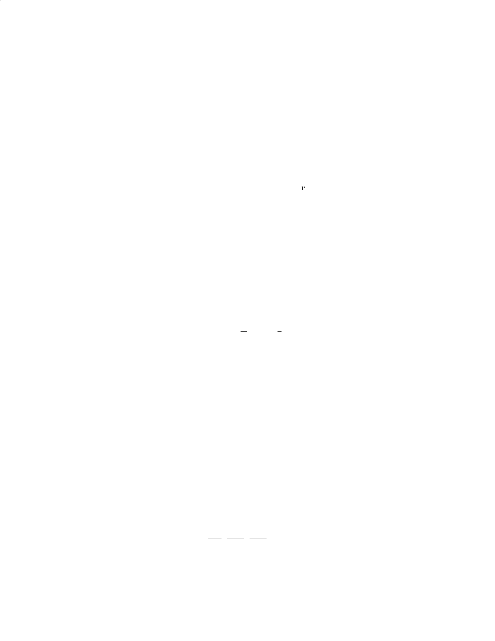
r′(t) = d
dt < t, t, t >=<1,1,1>
Step 2: Plug the Parametrization into the Vector Field We sub-
stitute the parametric form of the curve into the vector field F. Since
F = ¡2x, 3y, 4z¿, we have:
F(r(t)) = F(t, t, t) =<2t, 3t, 4t >
Step 3: Calculate the Dot Product F(r(t))
·
r’(t) We find the dot
product of F(r(t)) and r’(t):
F(r(t)) ·r′(t) =<2t, 3t, 4t > ·<1,1,1>= 2t+ 3t+ 4t= 9t
Step 4: Set Up the Integral to Evaluate the Line Integral The line
integral of F along C is given by:
ZC
F·dr=Z1
0
F(r(t)) ·r′(t)dt
ZC
F·dr=Z1
0
9t dt
Step 5: Evaluate the Integral We compute the integral:
Z1
0
9t dt = 9 t2
21
0
= 9 ·1
2= 4.5
Answer: The value of the line integral of the vector field F = ¡2x,
3y, 4z¿ over the curve C (parametrized by r(t) = ¡t, t, t¿ from t = 0
to 1) is 4.5.
Question 10
Problem:
Evaluate the line integral of the vector field F(x, y, z) = (2xy, x2−
yz, y2)over the curve r(t)=(t, t2, t3)from t= 0 to t= 1.
Solution:
Step 1: Parameterize the Curve
The given curve r(t)is already parameterized as:
r(t)=(t, t2, t3)
where truns from 0 to 1.
Step 2: Differentiate the Curve Parameterization
Differentiate r(t)with respect to tto find r′(t):
r′(t) = d(t)
dt ,d(t2)
dt ,d(t3)
dt = (1,2t, 3t2)
18
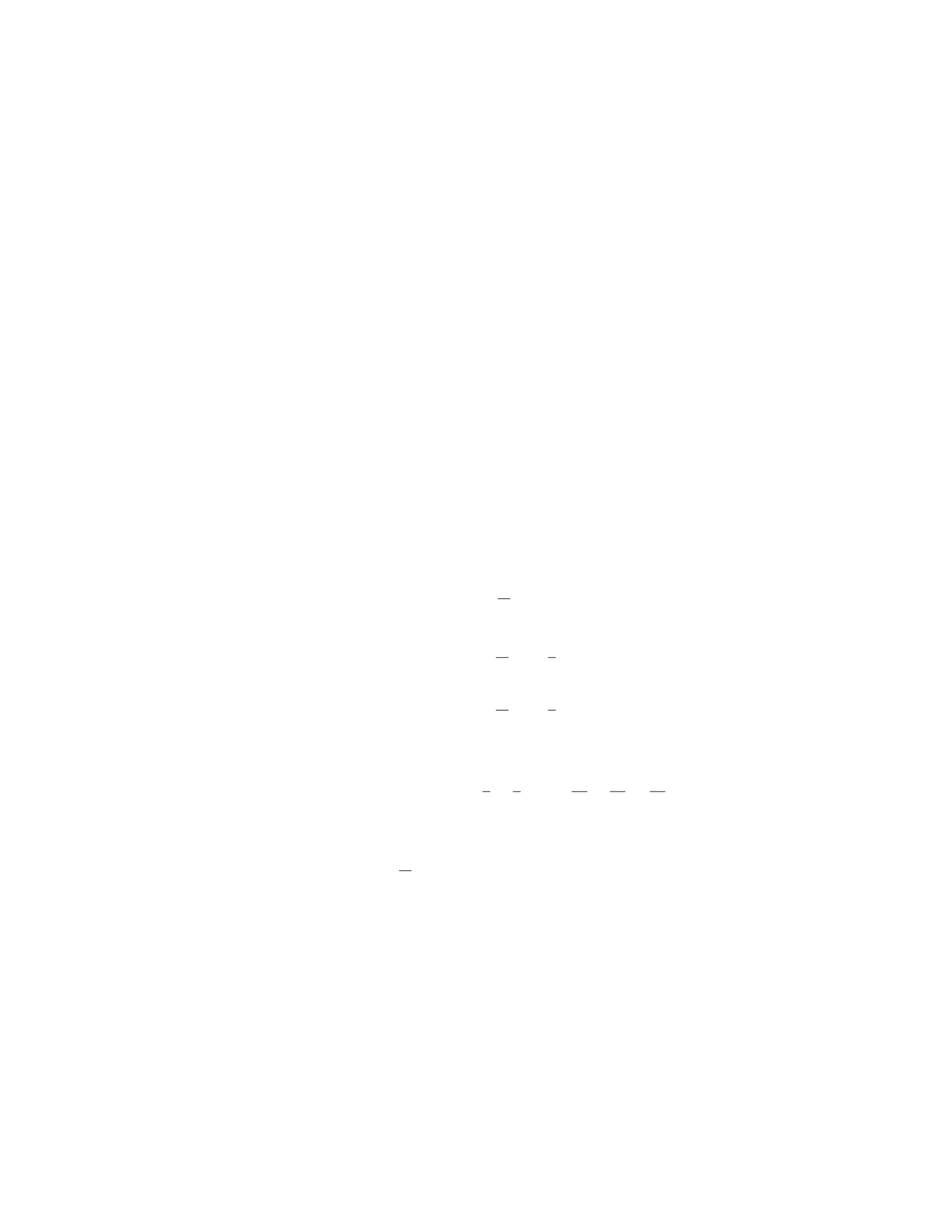
Step 3: Evaluate the Vector Field along the Curve
Substitute the parameterization r(t)into the vector field F(x, y, z):
F(r(t)) = (F(t, t2, t3)) = (2t·t2, t2−t3·t3,(t2)2) = (2t3, t2−t6, t4)
Step 4: Calculate F(r(t)) ·r′(t)
Compute the dot product of F(r(t)) and r′(t):
F(r(t)) ·r′(t) = (2t3, t2−t6, t4)·(1,2t, 3t2) = 2t3·1+(t2−t6)·2t+t4·3t2
= 2t3+ 2t3−2t7+ 3t6
= 4t3+ 3t6−2t7
Step 5: Integrate over the Interval
The line integral over the curve from t= 0 to t= 1 is given by the
integral of the dot product calculated in the previous step over the
interval:
Z1
0
(4t3+ 3t6−2t7)dt
Compute the integral term by term:
Z1
0
4t3dt = 4 t4
41
0
= 1
Z1
0
3t6dt = 3 t7
71
0
=3
7
Z1
0
2t7dt = 2 t8
81
0
=1
4
Combining these, we have:
Z1
0
(4t3+ 3t6−2t7)dt = 1 + 3
7−1
4= 1 + 12
28 −7
28 =25
28
Conclusion:
The value of the line integral of the vector field F along the curve
r(t)from t= 0 to t= 1 is 25
28 . Question 10 - Path Integral in Multivari-
able Calculus
Problem:
Evaluate the line integral of the vector field F(x, y, z) = (2xy, x2−
yz, y2)over the curve r(t)=(t, t2, t3)from t= 0 to t= 1.
Solution:
Step 1: Parameterize the Curve
The given curve r(t)is already parameterized as:
r(t)=(t, t2, t3)
19
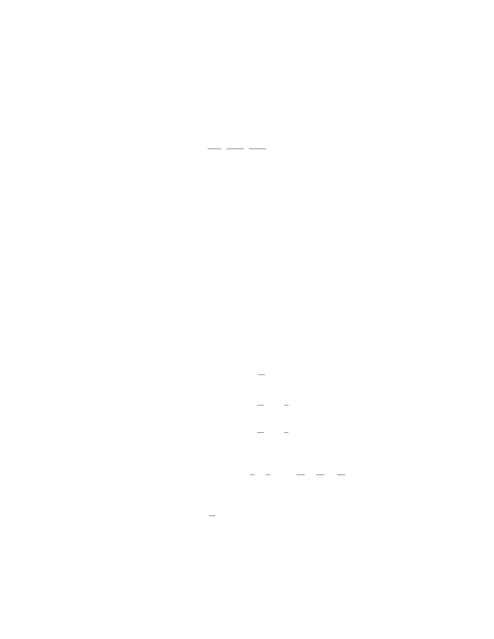
where truns from 0 to 1.
Step 2: Differentiate the Curve Parameterization
Differentiate r(t)with respect to tto find r′(t):
r′(t) = d(t)
dt ,d(t2)
dt ,d(t3)
dt = (1,2t, 3t2)
Step 3: Evaluate the Vector Field along the Curve
Substitute the parameterization r(t)into the vector field F(x, y, z):
F(r(t)) = (F(t, t2, t3)) = (2t·t2, t2−t3·t3,(t2)2) = (2t3, t2−t6, t4)
Step 4: Calculate F(r(t)) ·r′(t)
Compute the dot product of F(r(t)) and r′(t):
F(r(t)) ·r′(t) = (2t3, t2−t6, t4)·(1,2t, 3t2) = 2t3·1+(t2−t6)·2t+t4·3t2
= 2t3+ 2t3−2t7+ 3t6
= 4t3+ 3t6−2t7
Step 5: Integrate over the Interval
The line integral over the curve from t= 0 to t= 1 is given by the
integral of the dot product calculated in the previous step over the
interval:
Z1
0
(4t3+ 3t6−2t7)dt
Compute the integral term by term:
Z1
0
4t3dt = 4 t4
41
0
= 1
Z1
0
3t6dt = 3 t7
71
0
=3
7
Z1
0
2t7dt = 2 t8
81
0
=1
4
Combining these, we have:
Z1
0
(4t3+ 3t6−2t7)dt = 1 + 3
7−1
4= 1 + 12
28 −7
28 =25
28
Conclusion:
The value of the line integral of the vector field F along the curve
r(t)from t= 0 to t= 1 is 25
28 .
20

