



Advanced Plotting Assignment
Becca Arevalo 10/1/2023
Problem 5.4
Do a breakeven analysis for certain chemical product.
Fixed cost: $2.045 million per year
Variable cost:
-Material cost: 62 cents per gallon of product
-Energy cost: 24 cents per gallon of product
-Labor cost: 16 cents per gallon of product
let P be selling price in dollars per gallon. Selling price and sales quantitiy Q is Q=6x10^6-1.110^6P
Using the data...
-plot the fixed & total variable cost vs. Q
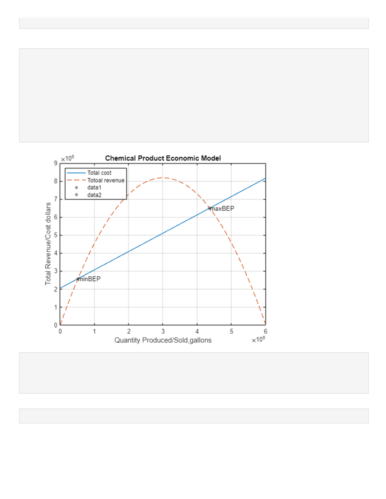
-graphically determine the breakeven point (with labels)
-Find the range of Q where production is profitable
-Find the value for the maximum profit of Q
Initialize Variables
clc, clear, close all
FC=2.045e6; %fixed cost in dollars per year
MC=.62;
EC=.24;
LC=.16;
Q=0:1:6e6; %quantity produced/sold in millions of gallons per year
Perform calculations
VC=MC+EC+LC; %variable cost in dollars per gallon producedTC=FC+Q.*VC; %return
total cost per year in millions $
P=(6e6-Q)./(1.1e6);%selling price in dollars per gallon sold
TR=Q.*P; %returns total revenue per year in millions
TC=FC+Q.*VC;
TP=TR-TC; %return profit per year in millions
Evaluate Results
idx=find(TP>0); %finding all possible indexes where TP is positive
min_idx=min(idx); %finding the frist index where TP is positive
max_idx=max(idx); %finding second index where TP is positive
minBEP=Q(min_idx); %first breakeven point in millions of gallons per year
maxBEP=Q(max_idx); %second breakeven point in millions of gallons per year
1
max_TR=max(TR);
Display results
plot(Q,TC,Q,TR,'--')
title('Chemical Product Economic Model')
xlabel('Quantity Produced/Sold,gallons')
ylabel('Total Revenue/Cost dollars')
legend('Total cost','Totoal revenue','location','Northwest')
grid on
hold on
plot(minBEP,TR(minBEP),'k*'),text(minBEP,TR(minBEP),'minBEP')
hold on
plot(maxBEP,TR(maxBEP),'k*'),text(maxBEP,TR(maxBEP),'maxBEP')
fprintf('The first breakeven point occurs at %3.0f million gallons and the second
breakeven point occurs at %3.0f. Production is only profitable between these two
points. ',minBEP,maxBEP)
The first breakeven point occurs at 515665 million gallons and the second breakeven point occurs at 4362335. Production is only profitable between these two points.
fprintf('The maximum profit possible is %3.0f',max_TR)
The maximum profit possible is 8181818
Problem 5.17
2

Initialize variables
clc, clear, close all
t=linspace(0,2*pi,1000);
sin_t=(10^-0.5.*t).*sin(3.*t+2);
cos_t=(7^-0.4.*t).*cos(5.*t-3);
plot functions/display results
plot(t,sin_t,t,cos_t,'--'), title('x(t) and y(t)'), grid on
xlabel('Angle in radians'),ylabel('cos and sin'), legend('sin(t)','cos(t)')
Problem 5.25
The Volume and Area of a sphere are
V=(4/3)pi*r^3
A=4*pi*r^2
Plot:
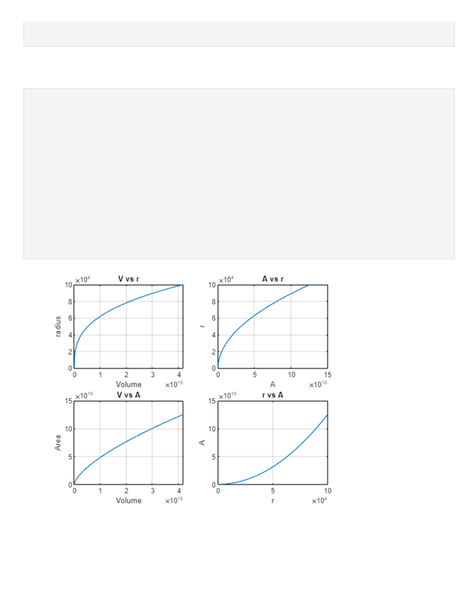
-V&A vs r 0.1<=r<=100m
-V&r vs A 1<=A<=10e4 m^2
clc, clear, close all
r=.01:.1:10e4;
3
V=(4/3)*pi*r.^3;
A=4*pi*r.^2;
Plot and Display results
subplot(2,2,1)
plot(V,r), title('V vs r'), grid on
xlabel('Volume'),ylabel('radius')
subplot(2,2,2)
plot(A,r), title('A vs r'), grid on
xlabel('A'),ylabel('r')
subplot(2,2,3)
plot(V,A), title('V vs A'), grid on
xlabel('Volume'),ylabel('Area')
subplot(2,2,4)
plot(r,A), title('r vs A'), grid on
xlabel('r'),ylabel('A')
Problem 5.26
current amount A or pricipal P is invested in a saving account paying an annual interest rate r
4

A=P(1+(r/n)^nt
n is the number of times per yer the interest is compounded
for continuous compounding
A=Pe^rt
Suppose $10000 is investeted initially at 2.5%. Plot A vs t 0<=t<=20 years for four different cases:
-continuous compounding
-annual compounding (n=1)
-quarterly compounding (n=4)
=monthly compounding (n=12)
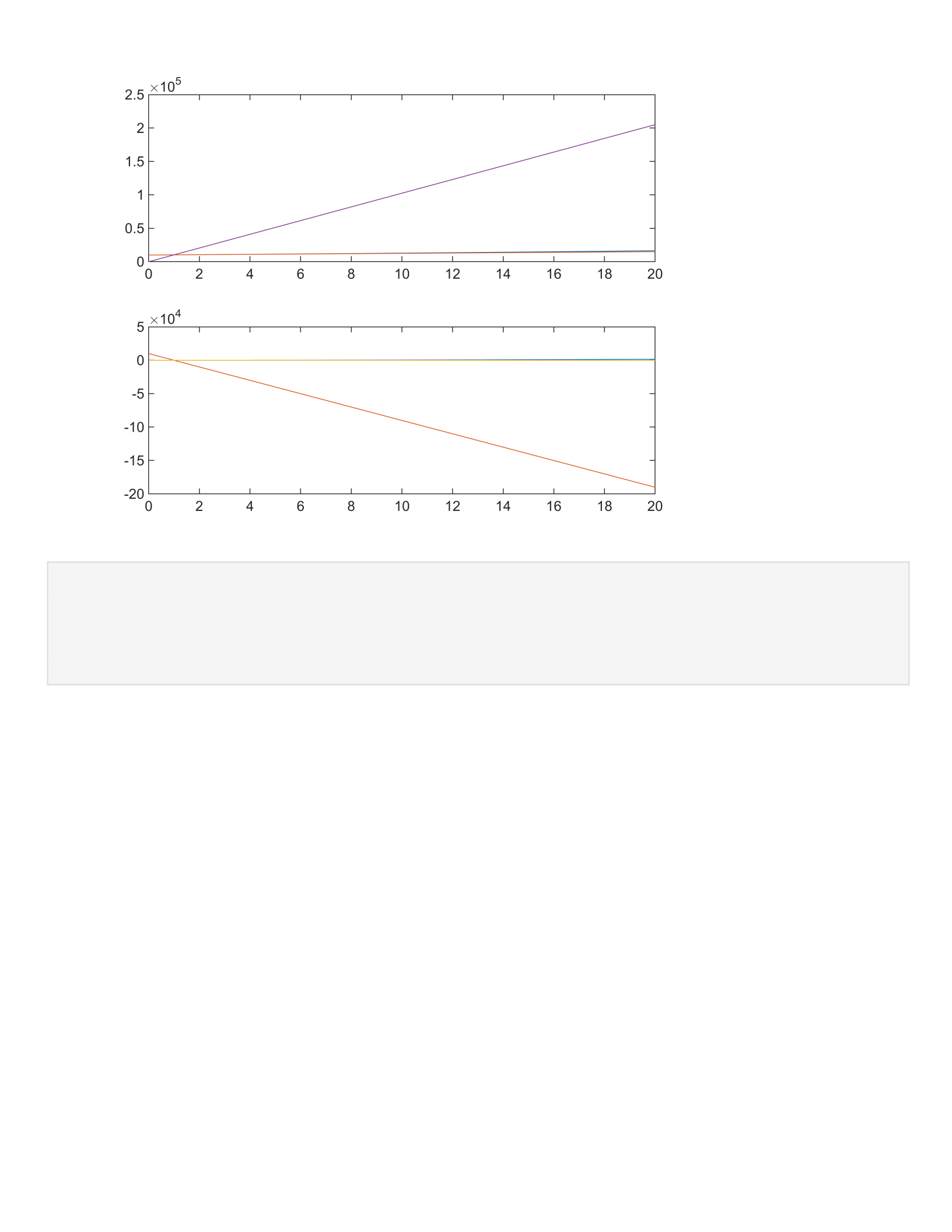
Plot and label each curve on the same plot, then on another plot do the difference between amounts obtained
from all four
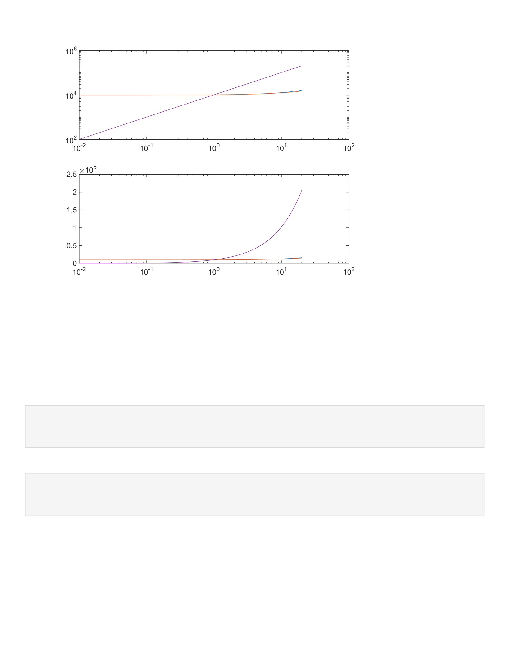
Then, repeat this again but plot A vs t on log-log and semilog plots.
Answer the question: "Which plot givess a straight line?"
Initailize Variables
clc,clear, close all
t=0:.01:20;
p=10000; %principal value
r=.025; %annual interest rate
Perform Calculations
CC=p*exp(r*t); %continuous compounding
AC=p*(1+(r/1).^1*t); %annual compounding
QC=p*(1+(r/4)).^4*t; %quarterly compounding
MC=p*(1+(r/12)).^12*t; %monthly compounding
Plot/ Display results
subplot(2,1,1)
plot(t,CC,t,AC,t,QC,t,MC)
subplot(2,1,2)
plot(t,CC-AC,t,AC-QC,t,QC-MC)
5
figure
subplot(2,1,1)
loglog(t,CC,t,AC,t,QC,t,MC)
subplot(2,1,2)
semilogx(t,CC,t,AC,t,QC,t,MC)
6
Problem 5.39
Plot the surface and contour plots of
z=x^2-4xy+6y^2
showing the minimum at x=y=0
Initialize variables
clc, clear, close all
[X,Y]=meshgrid(-5:.01:5); %defining the XY grid of interest
Z=X.^2-4*X.*Y+6.*Y.^2; %Z=f(x,y)
Display results
mesh(X,Y,Z), xlabel('X'), ylabel('Y'), zlabel('Z')
grid
title('Surface plot of z=X.^2-4*X.*Y+6.*Y.^2')
7

figure
contour(X,Y,Z), xlabel('X'), ylabel('Y'), zlabel('Z')
title('Contour plot of z=X.^2-4*X.*Y+6.*Y.^2')
8

Contour
plot
of
z=X.2-4*X.°Y+6.*Y.?
T
xe
9

