



Data and Methods regarding Workplace wellbeing
Methods
Regarding methodology, this study will conduct the research into three steps.
Firstly, a comparable data pool is established by using the propensity score matching approach.
It will classify them into four groups by observer’s job (the self-employed:1, employees: 0) and
by observer’s financial status (1: poverty, 0:non-poverty).
Secondly, the multiple-group analysis is used to seek the mean differences on job autonomy, job
anxiety, job depression and job Satisfaction among 4 groups. This aims to test H2: when individuals
incomes are below the poverty line, the self-employed have higher job autonomy and higher
workplace wellbeing than employees, and to answer the First question, do the self-employed always
feel happier (experiencing higher workplace wellbeing) than employeeseven they are in poverty?
Finally, to test H1: job autonomy has a positive relationship with workplace wellbeing, and H3:
poverty moderates the relationship between job autonomy and workplace wellbeing, the study
will conduct a SEM pathway analysis between job autonomy and workplace wellbeing among 4
groups, to investigate the changes of this relationship along with different level of financial
strain. Then, the interaction term (poverty*Job Autonomy) is introduced to test the moderating
impact of financial strain on the relationship between autonomy and job satisfaction.
Data and Measurements
The Understanding Society Panel Survey is the largest longitudinal survey of private
households in Great Britain that contains information on various areas of the respondents' lives,
ranging from income to household consumption, education, health, but also social and political
values. The data is sourced from the Fourth Wave of Understanding Society (The year 2013).
This dataset also covers a rich variety of employment status information for a representative
sample of the British population and is used wildly in the British research in the workplace

(Hughes, and Kumari,2016; Wheatley, 2016). The total sample is 20626 individuals including
the self-employed (N=2682) and the employees (N=17944).
Workplace wellbeing, the dependent variable. To address Warr’s model (2002), this study,
Workplace wellbeing is measured by three constructs: job satisfaction (pleasure-displeasure),
job anxiety (anxiety-comfort) and job depression (enthusiasm-depression). All items to
measure the variables are selected from the job satisfaction and working condition modules in
the fourth wave questionnaire. The question measures job satisfaction is: ‘how dissatisfied or
satisfied are you with your present job overall?’ It is effectively tracking an individual's job
satisfaction on a seven-point likert scale, ranging from ‘not satisfied at all’ (1) to ‘completely
satisfied’ (7). Job-related anxiety and depression were measured by scale consist of two three-
item subscales (all variable measurements are listed in Table 1). Both scales use a likert-type
response format and have demonstrated acceptable reliability and validity. Kerr, McHugh and
McCrory (2009) have used this measurement to test job stress and wellbeing.
Job Autonomy, the independent variable, is measured by a five-item scale from the work
condition module of understanding society 4th wave, This scale was originally designed for
Workplace Employment Relations Survey (WERS, 2004) to test the employees’ control power
on the five aspects of their jobs: How the work is done; The order in which tasks are carried
out; The pace of work; The tasks done in the job; Start and finish times ( see Table 1).
Poverty, the moderator, in this study, both the self-employed and employees are grouped by the
poverty line. Similar to the study conducted by Broughton and Richards (2016), the threshold
for poverty is 60% of median earnings of the population. This is also the threshold that is used
in many studies and policy reports to measure poverty. In previous research, both monthly pay
and hourly pay are adapted to measure poverty. Consistent with study of Broughton and
Richards (2016), the monthly income is applied to measure poverty as it can be seen as better
and more stable reflecting the total earnings that individuals have to spend. In 2012/13,
according to ONS, 60% of median monthly gross employee pay in the UK was £1,040. In this
study, this number is used as the threshold to create the dummy variable-poverty. Individual

with monthly income lower than £1,040, has been taken as poverty, coded with ‘1’, and
individuals with monthly income higher than £1,040, has been taken as non-poverty, coded
with ‘0’.
Demographic variables include age, sex, marital status and education. Since these variables
may confound the results, both variables are included in the model as well. For instance,
women tend to report greater job satisfaction than men, and they also tend to report more
psychosomatic symptoms (Jamal and Badawi 1995). Similarly, Jamal (1997) noted that age
might play an important role: older people report more health problems than younger people
do. Moreover, higher education may enlarge individual’s employment opportunity and hence
enhance the chance to find a more satisfying job. The single person experiences higher job
satisfaction due to the lack of family-work conflicts (Zimmerman, 2005). Therefore, from
previous research, all these demographic variables have significant associations with
workplace wellbeing. All these variables need to be controlled for in the matching approach
to establishing a comparable dataset, which will be explained in the next part. All the variable
measurement has been concluded in Table 3
Table 3 Variable Measurement
Item Variable label Scale
Workplace wellbeing
Job satisfaction 1 Job satisfaction 1: completely dissatisfied to 7: completely satisfied
Job Anxiety JA1 feels tense about job 1: never to 5: all the time
JA2 feels uneasy about job 1: never to 5: all the time
JA3 feels worried about job 1: never to 5: all the time
Job Depression JD1 feels depressed about job 1: never to 5: all the time
JD2 feels gloomy about job 1: never to 5: all the time
JD3 feels miserable about job 1: never to 5: all the time
Job Autonomy aut1 autonomy over job tasks 1: none to 4: a lot
aut2 autonomy over work pace 1: none to 4: a lot
aut3 autonomy over work manner 1: none to 4: a lot
aut4 autonomy over task order 1: none to 4: a lot
aut5 autonomy over work hours 1: none to 4: a lot
Poverty 1 1: poverty to 0: non-poverty

Matching approach
Table 4 Summary Statistics
the employees before T-test χ2 employees after T-test χ2
self-employed matching p-value p-value matching p-value p-value
N2682 17944 2682
Age mean 47.72 42.57 0.00 47.65 0.80
SD 11.85 11.81 11.73
Sex male% 0.64 0.45 0.00 0.64 0.88
Education degree 0.32 0.33 0.00 0.31 0.44
other higher 0.12 0.14 0.13
degree
A-level 0.22 0.22 0.21
GCSE 0.20 0.21 0.20
other 0.09 0.07 0.09
qualification
no qualification 0.06 0.04 0.05
Single yes% 0.23 0.28 0.00 0.22 0.36
Personal mean 2420.10 2314.25 0.04 2441.48 0.70
income
SD 2637.20 1632.34 1652.49
The matching approach selects a sub-data pool from the control group to create a mirror
image of the treatment group by control some key characters. Here the key characters also
called the demographic variables are highly related to dependent variables, which may affect
the judgments of group comparison (see Table 5). The computer selects the observation by
calculating the shortest distance between treatment group and control group, which is also
called the nearest neighbour matching. The same approach has been applied in the essay,
‘Life satisfaction and self-employment: A matching approach’ (Binder and Coad, 2013). This
study also use the Propensity score matching (Nonparametric Pre-processing for Parametric
Causal Inference), which is a statistical technique in which a treatment case is matched with
one or more control cases based on each case’s propensity score to double check two groups
are matched (see in Figure 3). To be more specified, this study control the rationale of the
treatment group population to control group population group as 1:1, so that is 2628(the self-
employed): 2628 (employees). After matched, it is obviously can see that the
75
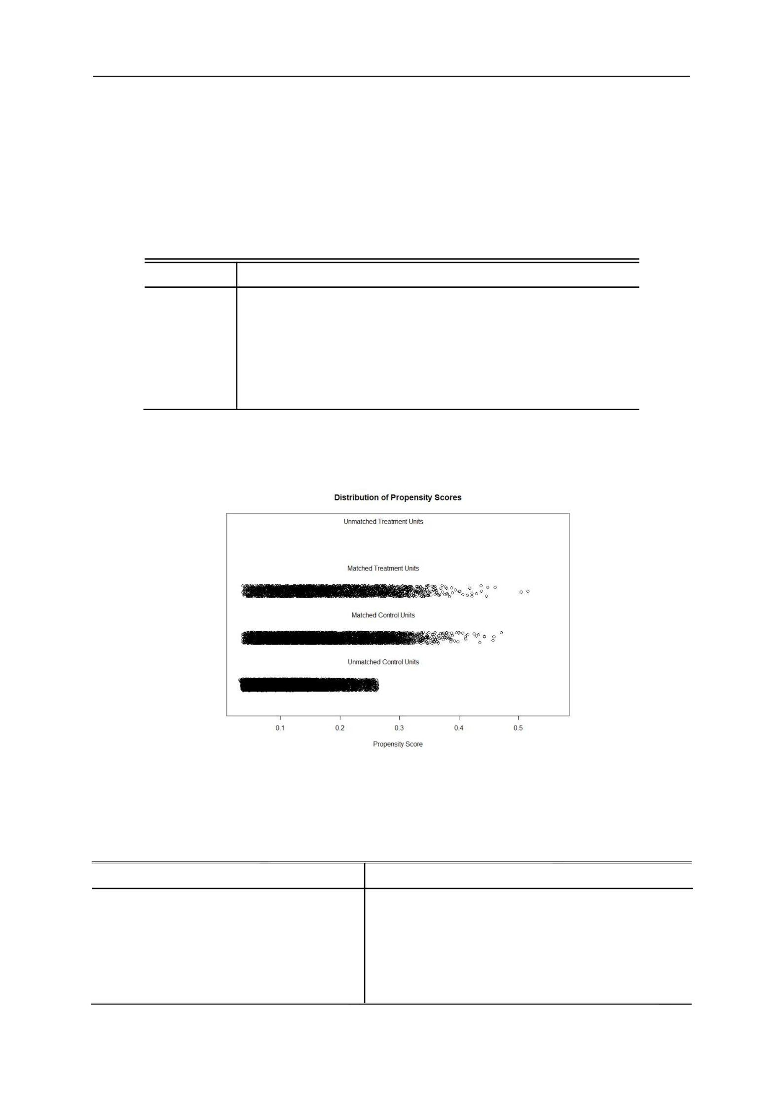
demographical differences has been largely reduced, the results of T-test and Chi-square test
p-values are revealed in Table 4, none of them is significant different in demographic
variables between the self-employed and employees. Also, the distribution of propensity
scores tends to similar between two groups after matching(see in Figure 3).
Table 5 Correlation Matrix
Job satisfaction JD1 JD2 JD3 JA1 JA2 JA3
Age 0.06*** -0.09*** -0.07*** -0.06*** -0.04*** -0.07*** -0.08***
Gender 0.03*** 0.07*** 0.02** 0.05*** 0.02** 0.02** 0.02*
Married -0.03*** 0.01* 0.02*** 0 0.03*** 0.03*** 0.02***
Education 0.04*** -0.12*** -0.07*** -0.12*** 0 -0.02** 0.02***
Personal Income 0.05*** 0.07*** 0.03*** 0.06*** -0.03*** -0.02* -0.04***
* p<.001
* p<.01
* p<.05
Figure 3 Distribution of Propensity Scores
Table 6 Financial Situation and Income Differences among Different Groups
Observation Personal Income(GBP)
Group1(the self-employed in poverty) 838 581.06
Group2(employees in poverty) 339 726.75
Group3(the self-employed without poverty) 1842 3258.55
Group4(employees without poverty) 2341 2707.02

From the Table 6, results indicate that the distribution of income of the self-employed is more
polarised than employees. The mean of income among lower-paid the self-employed is almost
one-third off than it among employees; (the self-employed in poverty:£581.06, employees with
poverty:£726.75). However, the share of the low-paid is dramatically larger in the self-
employed’ group, which accounts for 31.2%, while the in the employee's group, the number is
12.6%.

