


Remote Sensing Methods for Urban Forest Planning
Cities account for less than 3 percent of the global land surface but are home to
over 55 percent of the global population. The physical changes associated with
urbanization have altered the form, structure, and composition of the earth’s land
surface, affecting its thermal properties, energy balance, and biogeochemical cycles---
influencing the function of ecosystems and climate. Cities themselves are physically
diverse environments, demonstrating intraurban and interurban variability in terms of
their material composition and configuration, thermal characteristics, and ecological
capability, across a broad range of spatial, temporal, and geographic scales. (Upmanis
et al., 1998; Svensson & Eliasson, 2002; Huang et al., 2011; Hall et al., 2016; Jenerette
et al., 2016).
The disruptions to climate and ecosystems from urban-induced land use/land
cover change directly affect human health and increase the vulnerability of urban
populations to flooding, storms, heat, drought, sea-level rise, and damages to
infrastructures and buildings
(McMichael et al., 2006; United Nations Development Programme, 2006; Padowski &
Gorelick, 2014; Liu et al., 2017). The design and implementation of effective
adaptation and mitigation strategies, not only require a complete knowledge and
understanding of the unique structure and function of constituent subcomponents, but
of their interrelationships. This involves the widespread and comprehensive collection
of data of the urban landscape, at a granular level (Masser, 2001; Künzer & Dech,
2013; Tang & Li, 2014; Luderwitz et al. 2015). Many of the negative consequences of
urbanization are both local and global in effect; however, our understanding of the
processes, impacts, and their linkages across time and space is incomplete.

There is scientific consensus that the modifications to land use and land cover
associated with urbanization, have caused changes to the local microclimate of many
urban areas (Heidt ands Neef, 2008). This alters the micrometeorology of a city’s
built-up urban core relative to that of its rural surroundings, exhibiting differences in
solar radiation, air temperature, wind speed, relative humidity, cloud cover, and
precipitation. In general, urban areas experience higher temperatures, weaker winds,
and diminished solar radiation inputs, more air pollution, less relative humidity,
greater cloud cover, and increased precipitation compared to their rural outskirts
(Gilbert, 1989; Heidt and Neef, 2008). These climatic differences are the result of
complex, diverse, and often collective interactions between the natural and built
environment.
Analytical methods for studying the role of forests in the urban environment
include applications remote sensing data and technology, and geospatial analysis.
Remote sensing is the acquisition of information about an object or phenomena that is
done without making physical contact with it. Remote sensors collect data of the
physical characteristics of an area or object by detecting its reflected or emitted
electromagnetic radiation at a distance from the targeted area. Remote sensing
represents the only practical means to acquire large areas of data of the earth’s surface
and atmosphere in a globally consistent and economically feasible manner (Voogt &
Oke, 2003; Imhoff et al., 2010; Tang & Li, 2014). The improved spatial and temporal
coverage associated with remote sensing technology and methods has vastly improved
the ability to observe and record data of natural phenomena in both the long and short
term. Additionally, remote sensing has made it possible to collect data of inaccessible
and dangerous locations. Remote sensing instruments are deployed on three types of

platforms: 1) ground based, 2) airborne, and 3) satellite. The platform chosen for a
particular sensor is determined by several factors including: the distance of the sensor
to the object of interest; periodicity of image acquisition; timing of image acquisition;
location; and extent of coverage.
Remote sensing-based solutions can be used to promote more sustainable
urban forestry management practices that lead to more resilient forests in the future.
Remote sensing data and technology can provide critical information for urban
forestry management, such as monitoring tree growth, identifying areas of forest
stress, and tracking forest cover changes. This approach can help urban foresters to
make informed decisions, optimize resource allocation, and promote more sustainable
forestry management practices.
One of the key applications of remote sensing in urban forestry management is
monitoring tree growth. Remote sensing data can be used to track tree canopy cover
and changes in forest structure over time. For example, LiDAR (Light Detection and
Ranging) technology can provide detailed 3D information about forest structure and
tree height, allowing for more accurate estimates of forest biomass and carbon storage
(Beland et al., 2018). This information can be used to identify areas where tree growth
is lagging and prioritize interventions to improve tree health.
Another application of remote sensing in urban forestry management is
identifying areas of forest stress. Remote sensing data can be used to detect changes in
tree health, such as leaf chlorophyll content, water content, and photosynthesis rates
(Zhao et al., 2016). This information can be used to identify areas of forest stress, such
as those affected by drought or insect infestations. Early detection of forest stress can

help urban foresters to take proactive measures to mitigate the effects of stress on
forest health.
Remote sensing-based solutions can also be used to track forest cover changes
and identify areas of forest loss. Satellite imagery can provide information about
changes in forest cover and fragmentation over time. This information can be used to
identify areas where forest loss is occurring and prioritize conservation efforts (J.
Zhang et al., 2016). Additionally, remote sensing can be used to identify areas with
potential for reforestation or afforestation, promoting sustainable urban forestry
practices.
The most challenging aspect for most urban remote sensing applications,
relates to the spectral heterogeneity and morphological complexity of the urban fabric
(Shen et al., 2016). The spectral heterogeneity arises from the enormous diversity of
different materials forming the urban landscape. Some urban surfaces (e.g., bare soil
and specific construction materials of buildings or pavements) are difficult to
differentiate from each other, when comparing their spectral signature. High spatial
resolution imagery (e.g., from manned or unmanned aircraft; or from satellites such as
IKONOS, QuickBird, Worldview) provides new opportunities to map detailed urban
areas at a fine scale by providing more detailed observations of the Earth (Cao et al.,
2010; Labchoon et al., 2017). The diversity of scale and shape of the structural
elements of the urban environment contribute to its morphological complexity. A
sensor system with a very high spatial resolution is necessary to capture the
morphological properties of urban features more accurately. An increase in spatial
resolution significantly expands the range of the detected spectrum and the observable
heterogeneity within the specific object types. However, urban features are

fundamentally composed of groups of pixels with similar spectral signatures (Voogt &
Oke, 2003; Zhou et al., 2019).
Research Objectives & Novelty
Urban environments are complex ecosystems where the interplay of natural
and built elements significantly influences the quality of life, environmental
sustainability, and resilience to climate change. Recent advancements in technology
and analytical methods have opened new avenues for understanding and managing
these ecosystems more effectively. Remote sensingbased solutions offer a cost-
effective and efficient means of gathering detailed spatial and temporal information
over large areas that would otherwise be difficult or impossible to obtain using
ground-based field survey methods. In the context of this research, remote sensing
data and technology are used to provide critical information for the effective
environmental planning, managing, and monitoring of urban forests. An overall goal
of this research is to improve on the knowledge and understanding of the intricate
dynamics of urban forest ecosystems and develop new tools to assist with their
management.
To achieve these goals, this three-part investigation introduces new approaches
for the comprehensive quantification and spatial mapping of tree shade as a superior
alternative to UTC coverage metrics, the application of hierarchical linear modeling to
explain relationship between surface temperature and nested land use, land cover
variables across different spatial scales, and for assessing the efficacy and feasibility
of Unmanned Aircraft Systems (UAS) for specific urban forest management tasks.
Specifically, the research objectives include:

1. Apply new approach for mapping and evaluating the effects of UTC shade on
surface temperature at multiple local scales. Show that tree shade metrics
reveal significant microclimatic insights that are not discernible through
traditional UTC coverage metrics at sub-meter scales. Accurately measure the
reduction in surface temperatures from UTC shade on different types of urban
surface cover.
2. Use maximum likelihood HLM estimation to evaluate the contextual and
climatic effects of neighborhood-level land use factors on local-scale average
surface temperature of sidewalks within individual nested census block groups
(CBGs). Identify the Level 1 and
Level 2 variables that best explain variance in mean sidewalk surface
temperature.
3. Review the current state of practice and knowledge related to the use of
Unmanned Aircraft Systems (UASs) in urban forestry. Ascertain the efficacy of
using UASs for common urban forestry tasks, such as species inventory, tree
health monitoring, and outbreak identification. Determine whether UAS-based
approaches might be both technically feasible and cost-competitive with field-
based methods.
Remote sensing data and technology are used to provide critical information
for planning, managing, and monitoring urban-forest environmental systems. Each
study combines the use of remote sensing data or technology with various methods for
geospatial and quantitative analysis, to produce valuable insights into the optimization
of urban forest management and planning for more resilient and livable cities, while
contributing to a more nuanced understanding of urban ecological dynamics.

Chapter Summaries
Article 1: Tree Shade Explains Urban Heat better than Tree Canopy at Microscale
using UAS
Given the significant impact of urban tree canopy (UTC) on local climates,
there is an urgent need for metrics that encompass the structural and functional
qualities of UTC, not just canopy coverage. This study introduces a method for
detailed quantification and mapping of tree shade across urban areas, illustrating its
effectiveness in identifying microclimates and predicting urban heat on various spatial
scales. Our aim was to analyze spatial and temporal patterns of UTC and its shade,
determining the best metric for predicting urban heat by studying its correlation with
land surface temperature in Denver, Colorado, at two scales: a coarse
assessment using Landsat 8 data with 30-meter resolution and a fine-scale analysis
using UASderived thermal imagery at 41-centimeter resolution. The high-resolution
UAS data enabled precise measurements of UTC shade's cooling effects on different
urban surfaces, such as turf grass and impervious materials, which showed significant
temperature reductions (6.7°C and 6.8°C, respectively). These findings highlight the
critical cooling benefits of strategically placed tree shade and the need for advanced
UTC metrics that accurately assess its cooling impact and role in urban climate
management.
Research
Questions
(1) What is the relationship
between remotely sensed measures of
land surface temperature and the
coverage metrics of UTC and UTC
shade?
(2) Which coverage metric is
the better predictor of land surface
temperature, as an indicator of urban
heat?
(3) How are these relationships
influenced by the specific spatial scale
used for analysis?
Approach
Uses remote sensing and geospatial analysis to
simulate UTC shade effects. Empirically quantifies
and validates the thermal impact of this shade effect
on the surface temperature of different urban land

cover.
Intellectual
Merit
Demonstrates the superiority of UTC shade metrics
over UTC coverage, for predicting urban heat (land
surface temperature) at sub-meter scale. Accurately
measures this thermal effect for Denver, Colorado.
Article 2: Application of Hierarchical Linear Modeling to the Analysis of Urban
Microclimate
The critical interaction between urban infrastructure and climate dynamics
underscores the necessity for refined urban planning strategies, particularly in the
context of the Urban Heat Island (UHI) effect. This study examines the significant
influence of material composition and spatial configuration on urban climate
dynamics, focusing on the role of impervious surfaces and urban greenery in
modifying urban thermal environments. It delves into the nuanced role of urban trees
and other vegetation in regulating climate, emphasizing their strategic use to lessen
solar loads on buildings and improve comfort in public spaces. By modifying land
cover and land use, urban planners can influence microclimates within cities,
mitigating the UHI effect through various scales of intervention—from the types of
surfaces in urban designs to the density and arrangement of green spaces.
Furthermore, this research discusses the importance of multiscalar statistical
approaches in urban planning. By integrating scale-sensitive strategies, urban planners
can address the complexity of urban forms and their varied climate patterns, thereby
enhancing the efficacy of interventions aimed at climate adaptation and sustainability.
Using the mean surface temperature of sidewalks nested within census block groups
(CBGs) as the dependent variable in a hierarchical linear model (HLM), we employ an
ordinary element of the urban environment to advance the understanding of the

complex interactions between microclimate and the green and grey components of
urban infrastructure. Sidewalks within census block groups were selected to serve as a
vital instrument for gauging urban land surface temperatures (LST), given their
pervasive presence and direct interaction with pedestrian activity. At two different
levels of spatial scale, we examine the impact of independent variables representing
different land cover and land use characteristics, in relation to the dependent variable
representing LST.
Research
Questions
(1) Which census block group-scale land
cover (Level 1) factors explain the within-group
variance in CBG sidewalk mean land surface
temperature (i.e., lower-level direct effects)?
(2) Which neighborhood-scale land use
(Level 2) factors explain the variance in across-
group intercepts (examining cross-level direct
effects)? Do models including Level 2 factors
improve the prediction of CBG sidewalk mean
land surface temperature, over models using only
Level 1 factors?
(3) Which combinations of census block
group-scale land cover (Level 1) factors and
neighborhood-scale land use (Level 2) factors
explain the variance in across-group slopes
(examining cross-level interaction effects)?
Approach
Uses remote sensing data, geospatial analysis, and HLM to
dissect the multi-scalar dynamics of urban climatology, revealing
the meaningful role of land cover factors at the CBG-scale and
land use factors at the neighborhood-scale for moderating urban
heat.
Intellectual
Merit
The potential for interacting covariates and unmeasured
confounders at both the CBG and neighborhood scales highlights
the inherent complexity in modeling urban climate dynamics,
underscoring the importance of exploring sophisticated analytical
methods like HLM for such purposes.
Article 3: Assessing the utility and cost-effectiveness of Unmanned Aircraft Systems
(UAS) in common urban forestry applications

This paper reviews the current state of practice and knowledge related to the
use of Unmanned Aircraft Systems (UASs) in urban forestry. It explores findings on
the feasibility and cost-effectiveness of using UASs for common urban forestry tasks,
such as species inventory, tree health monitoring, and outbreak identification. Small
UAs (weight < 55 lbs.) equipped with a variety of different sensor payloads were used
to collect urban forest data from multiple sites. Then geospatial and statistical analysis
techniques were used to test the ability of different sensors to identify tree species and
to determine which trees may be diseased or stressed. Interviews with UAV and urban
forestry professionals were then used to estimate costs for remote and field-based
methods. This information was used to assess whether UAS-based approaches might
be both technically feasible and cost-competitive with field-based methods.
Research
Questions
(1) How accurately can multiple deciduous tree species be
discriminated at the individual tree level within urban
landscapes using multispectral data collected via small-
airframe UAS mounted with lightweight sensors (weight < 55
lbs.)? (2) Is UAS-remote sensing a viable and cost-
effective alternative to traditional ground-based urban forest
inventories, both in terms of distinguishing specific tree
species and in diagnosing and quantifying tree health stress
levels?
Approach
The research process involves designing and executing UAS
flights with a variety of sensors to gather urban tree data,
statistical analysis of collected data to gauge the accuracy of
tree species identification and health assessment, the collection
of interview data on the costs of conducting both ground- and
UASbased methods, and a comparison of their cost-
effectiveness based on a synthesis of collected information.
Intellectua
l
Merit
The study enhances the domain of UAS-driven urban forest
data acquisition, pinpointing which tasks can be efficiently
replaced and which necessitate further technological
advancements or cost optimizations.

CHAPTER II
Article 1: Tree Shade Explains Urban Heat better than Tree Canopy at Microscale
using UAS

ABSTRACT
Considering the critical impact of urban tree canopy (UTC) on local climate
conditions, there is a pressing need for advanced metrics that capture the structural and
functional aspects of UTC beyond mere canopy coverage. This research demonstrates
a methodology for the comprehensive quantification and spatial mapping of tree shade
across an entire urban area, showcasing its utility in delineating urban microclimates
and predicting urban heat across a continuum of spatial scales. The objective was to
quantify and map the spatial and temporal patterns of urban tree canopy and urban tree
canopy shade, and to evaluate which coverage metric is the better predictor of urban
heat by examining its relationship with land surface temperature at two different
spatial scales of analysis, using a case study set in Denver, Colorado. The study
consists of two independent investigations: 1) a coarse-scale assessment that uses
conventional land surface temperature data sourced from Landsat 8 with a spatial
resolution of 30 meters (98.4 feet), and 2) a fine-scale assessment that uses land
surface temperature data derived from UAScollected thermal infrared imagery with a
spatial resolution of 41 centimeters (1.3 feet). Additionally, the very high resolution of
the UAS-collected imagery, both spatially and spectrally, allows researchers to
precisely measure the cooling effects of UTC shade on the surface temperature of
different urban land cover, specifically, turf grass and impervious surface. We found
that tree shaded turf and impervious surfaces exhibit substantial reductions in surface
temperature (approximately 6.7°C and 6.8°C, respectively), compared to their exposed
counterparts. This evidence underscores the enhanced cooling benefits of strategically
integrated tree shade in urban environments, highlighting the necessity for refined

UTC metrics that accurately reflect the canopy's cooling efficacy and its role in urban
climate regulation.
TABLE OF CONTENTS
INTRODUCTION………………………………………….
…………………………………....14
METHODS…………………………………………………….
………………………...............20
Analytical Approach………………………………………….
……………………………...20
Study Area and
Sampling……………………………………………………………………22
2D Land Cover Variable Creation……………………………….
…………………………..25
3D Shade Simulation and Shade Variable Creation……………….
………………………...27
Statistical Methods……………………………………………….….
……………………….32
Coarse-Scale Assessment…………………...……………..
……………………………..32
Fine-Scale Assessment ...…...………………………………..……………………..
……34
RESULTS………………………………………………….………………..
…………………...38
Coarse-Scale Assessment ……....……………………………………………...
…………...38
Fine-Scale Assessment ……….……...………..
……………………………………………41
DISCUSSION……………………………………….
…………………………………………...47

CONCLUSION………………………………………...
………………………………………...52
REFERENCES…………………………………………......………….
………………………...53
INTRODUCTION
Urban areas are recognized for creating distinctive microclimates, which often
exhibit higher temperatures than those found in their rural surroundings. The term
Urban Heat Island
(UHI) is used to describe this phenomena (Landsberg, 1981; Oke, 1982, 1987; Voogt
& Oke, 2003), which is associated with numerous adverse outcomes for urban
populations including diminished thermal comfort and higher heat-related health risk,
increased energy consumption, impaired air and water quality, loss of biodiversity,
accelerated degradation to infrastructure, and higher economic costs (Tan et al., 2016;
Santamouris & Kolokotsa, 2015). Factors such as city topography, spatial layout,
building density, configurations of open spaces, construction materials, urban air flow,
and anthropogenic heat from transportation and industry significantly contribute to the
formation of UHIs (Taha, 1997; Akbari et al., 2001; Grimmond, 2007). Still, the main
cause of UHI are the changes to land use and land cover characteristics, primarily
from the depletion of vegetated cover, due to urban development. During this process,
the naturally occurring land cover is replaced by impervious surface made from
synthetic materials like metal, concrete, and asphalt (Oke, 1982; Heidt and Neef,
2008; Tang & Li, 2014). As a rule, urban environments absorb twice as much heat
compared to more vegetated rural areas (EPA, UHI Basics, 2008).

In an urban setting, vegetation and greenspace moderate the effects of UHI,
and have been implemented as effective strategies for mitigating urban heat (Galagoda
et al., 2018;
Aboelata & Sodoudi, 2020). Vegetation influences urban microclimate by decreasing
LST and Ta in four ways: 1) by reducing the short-wave solar radiation absorbed by
the urban fabric with higher albedo relative to synthetic features; 2) by reducing the
sensible heat flux via shading; 3) by actively cooling areas with the conversion of heat
via transpiration and the evaporation of water (evapotranspiration); and 4) by
enhancing air flows with the generation of atmospheric convection (Armson et al.,
2012; Gillner et al., 2015; Crum & Jenerette, 2017).
The lower part of the atmosphere, occupied by cities, is very sensitive to small-
scale surface-plant-air interactions. The replacement of natural vegetation with
synthetic building materials constitutes a removal of the active cooling effects of
evapotranspiration. The lower albedo of the replacement building materials means it
reflects less and absorbs more incident solar radiation relative to replaced vegetation,
while its lower emissivity values are indicative of its greater capacity for the retention
of absorbed energy. Some of the absorbed energy is emitted thermally as heat and is
perceived as elevated LST, and increased Ta in the lowest layer of the urban
atmosphere. After sunset, in the absence of solar forcing, the remaining stored long-
wave heat is emitted. The geometry of urban morphology combined with the reflection
characteristics of urban surfaces can cause an urban canyon effect that blocks the
escape of emitted long-wave heat, while disrupting the wind flows that create
convective cooling (Oke 1982; Tang and Li, 2014; Crum and Jenerette, 2017). The
numerous complexities of the surface heat exchange processes and the heterogeneity

of urban fabric have resulted in a diversity of methods for measuring thermal effects
both within and between cities. For example, the effects of land cover on LST can be
observed at microscales of less than 10 m, while the effects of land cover on Ta are
frequently observed at moderate spatial scales of 20-500 m (Jenerette et al., 2016).
There are still knowledge-gaps regarding the specific heat reduction
performance of different types of vegetation interventions and interactions between
green and grey infrastructure in various cities at different spatial scales (i.e. local
versus city scale). The preponderance of past research shows that vegetation cooling
effects is predominantly driven by shading (Hoelscher et al., 2016; Speak et al., 2020;
Rahman et al., 2020), with only a small proportion due to evapotranspiration (Y. J.
Huang et al., 1987; Taha, 1997). For example, Shashua-Bar and Hoffman (2000) found
that shading accounted for 60 % of the total cooling effect of urban vegetation and
Cameron et al. (2014) found that shading contributed up to 80 %. McPherson et al.
(1988), showed dense shade on all surfaces of homes reduced peak cooling loads 31-
49% depending on the climate. This is supported by the work of Akbari et al. (1997)
illustrating the impacts of tree shading on residential energy consumption, which
demonstrates that trees can reduce surface temperatures (within the shaded area) by as
much as 20–45 °F (11–25 °C). Research from Brown and Gillespie (1995)
demonstrates that, under consistent conditions, shaded areas can be 20-40°C cooler
than their sunlit counterparts across various global climates. In comparison with trees,
turf is less effective in terms of cooling efficiency by 18% (described with LST) due to
the lower canopy coverage and less soil moisture accessed by plant roots (Rahman et
al., 2021).

Most previous research on the cooling effects of urban tree canopy (UTC)
shade were mainly conducted at a small spatial scale and focused on a few buildings
and trees, at a single point in time (Heisler, 1986; Akbari et al., 1997, 2001; Akbari,
2003; Armson et al., 2012; Berry et al., 2013; Middel et al., 2016; Morakinyo & Lam,
2016; Hwang et al., 2017), leaving a dearth of studies conducted at larger spatial
scales such as city scale. Recently, a few papers explored tree shade distribution using
tree height data at the city scale. Aleksandrowicz et al. (2020) utilizes a tree cover and
a building elevation raster to compute ground-level shades over streets and open
spaces in Tel-Aviv, Israel. Yu et al. (2020), used geospatial and empirical modeling to
simulate and measure the cooling effect of UTC shade, and evaluate its ability to
explain the variation in land surface temperature (LST), for New York City, NY and
Tampa Bay, FL. One major limitation of this study stemmed from the spatially coarse
30-meter LST data, which had been resampled from its original 120-meter footprint.
Both spatial scales are problematic for the analysis of heterogenous urban settings
because they allow for the mixing of multiple types of land cover within a single
surface temperature pixel.
Urban tree canopy (UTC) cover is an important metric for estimating overall
urban forest benefits, including cooling effects (Nowak & Greenfield, 2012). UTC
coverage (e.g. UTC area or % UTC) is the proportion of land area occupied by tree
crowns, when viewed from above, and serves as a baseline for setting community tree
canopy goals and measuring progress (Nowak et al., 1996). Some US cities aim to
increase UTC by 50–100% from current levels (Leff, 2016) to maximize future tree
benefits. UTC coverage metrics have been used to quantify tree shade at city scale
(Lee et al., 2016; Li et al., 2018; Aleksandrowicz et al., 2020; Yu et al., 2020).

However, coverage metrics only capture the 2-dimensional cover of tree crowns,
which cannot accurately represent the distribution of projected shade, as it lacks the
vertical dimension needed to estimate the 3D spatial extent. Additionally, UTC does
not consider the movement of the sun and therefore cannot account for the temporal
patterns of tree shade.
UTC coverage metrics are usually obtained with remote sensing, including
imagery generated from LiDAR data and/or high-resolution digital aerial photographs
or satellite images. The accuracy of UTC simulation and quantification has steadily
improved with the use of 3D
LiDAR data and the application of object-oriented classification techniques advanced
by the University of Vermont Spatial Analysis Laboratory. The advantage of LiDAR is
that it essentially sees through shadows, resulting in a more accurate and visually
coherent representation of a city’s tree canopy (O’Neil-Dunne et al., 2013).
Remote sensing in the thermal infrared (TIR) part of the electromagnetic
spectrum provides information on reflected longwave radiation needed to compute
land surface temperature. The signal is inversely proportional to the evapotranspiration
of UTC and can provide an indirect estimate of the surface energy balance and plant
water stress (Delogu et al., 2018). TIR data have been used extensively to document
the effects of vegetation cover and structure on surface temperature and emissivity
over an urban area (Weng et al., 2004; W. Zhou et al., 2011; Coutts et al., 2016; X. Yu
et al., 2017; W. Li et al., 2017). The most widely accepted range for TIR remote
sensing in vegetation studies is 3–14 μm, divided into the MWIR (3–5 μm) and the
LWIR (8–14 μm). The MWIR receives both emitted radiation from Earth and reflected
radiation from the Sun, while the LWIR is dominated by the emitted component

(Jensen & Hardin, 2005). Urban green spaces and trees are known to interact with
solar IR radiation in a way that is dramatically different to the way they deal with
visible (VIS) solar radiation via photosynthesis. Deng et al. (2018) characterized the
crown-level IR radiative performance of 10 lime trees and found that measured crown
transflectance changed substantially with solar time. These findings have significant
implications for species selection and control of environmental stress factors in urban
microclimates. Finally, Speak et al. (2020) used thermal imaging to quantify the effect
of solitary shade trees on the surface temperature of three common urban surface
types, i.e., asphalt, porphyry, and grass.
One of the most critical barriers to remote sensing applications in urban
forestry is the lack of timely data collection over target areas. The use of Unmanned
Aircraft Systems (UASs) remote sensing techniques, emerges as a promising solution,
offering a way to bypass the limitations of traditional remote sensing methods by
providing high-resolution, cost-effective data collection (Colomina & Molina, 2014;
Banu et al., 2016). Stability, safety, control, reliability, and autonomy of UAS,
combined with the specificity of the sensors, are the factors that allow successful
implementation of this new platform for remote sensing of urban forests.
Despite recent innovations, the use of UAS and very high resolution TIR imagery to
quantify the thermal effect of shades projected by urban trees remains an
underexamined application.
This research demonstrates a methodology for the comprehensive
quantification and spatial mapping of tree shade across an entire urban area,
showcasing its utility in delineating urban microclimates and predicting urban heat
across a continuum of spatial scales. The objective was to quantify and map the spatial

and temporal patterns of urban tree canopy and urban tree canopy shade, and to
evaluate which coverage metric is the better predictor of urban heat by examining its
relationship with land surface temperature at two different spatial scales of analysis,
using a case study set in Denver, Colorado. The study consists of two independent
investigations: 1) a coarse-scale assessment that uses conventional LST data sourced
from Landsat 8 with a spatial resolution of 30 meters (98.4 feet), and 2) a fine-scale
assessment that uses LST data derived from UAS-collected thermal infrared imagery
with a spatial resolution of 41 centimeters (1.3 feet). Additionally, the very high
resolution of the UAS-collected imagery, both spatially and spectrally, allows
researchers to precisely measure the cooling effects of UTC shade on the surface
temperature of different urban land cover, specifically, turf grass and impervious
surface. This research will address the following questions:
(1) What is the relationship between remotely sensed measures of land surface
temperature and the coverage metrics of UTC and UTC shade?
(2) Which coverage metric is the better predictor of land surface temperature,
as an indicator of urban heat?
(3) How are these relationships influenced by the specific spatial scale used for
analysis?
METHODS
Analytical Approach
The fundamental modeling approach is to establish a statistical relationship
between microclimatic variation in land surface temper temperature and the
heterogeneous urban environment characterized by various 2D and 3D representations
of different types of land cover, and the shade cast by buildings and trees for a

specified location, date, and time. The methodology for both the coarse-scale and fine-
scale analyses are comprised of the same three primary steps including: 1) the creation
of 2D variables from classified land cover representing buildings, trees, turf grass, and
impervious surface; 2) modeling of shade in 3D and the calculation of specified shade
variables; and 3) the statistical analysis to quantify the relationship between the
change in LST (dependent variable), different types of land cover and shade variables
(independent variables).
The LST data for the coarse-scale analysis study area was obtained from
Landsat 8 Thermal Infrared Sensors (TIRS) Analysis Ready Data (ARD), with a
resampled 30-meter spatial resolution, for August 4, 2017. This was a hot day, with
minimal cloud cover, during summer. The date selection was influenced by our warm-
weather research objectives and the limited temporal availability of Landsat 8 thermal
imagery. Landsat 8 data has been widely used across the world in urban surface
temperature research (Park et al., 2021). The ARD images are post-processed to the
highest scientific standards required for direct use in land cover change assessment.
Landsat uniquely provides large-scale land surface temperature (LST) data with each
30-meter pixel representing an average of the local thermal environment. Very high-
resolution land cover and shade variables are generated at a granular scale of 0.5 to 1
meter. However, to align with the Landsat LST data, these variables are subsequently
aggregated to a 30-meter resolution. This aggregation yields an average over the
conditions present within each Landsat pixel, facilitating direct compatibility with the
LST measurements. Thus, the integrated dataset effectively reflects the combined
influence of land cover diversity and distribution within the scope of a single LST
pixel.

The LST data for the fine-scale analysis was acquired with UAS on September
4, 2019, under cloud-free conditions. Specifically, a DJI Matrice 600 hexacopter
airframe with the
Micasense Altum sensor as payload, distinguished by six spectral bands (Blue, Green,
Red, Red Edge, Near Infrared, Thermal), was used for the collection of very high-
resolution thermal and multispectral imagery, at 41 centimeters (16.14 inches) and 2.6
centimeters (1.02 inches), respectively. The September 2019 mission had an earlier
start time of 9:30 AM. Ideally, UAS missions are flown between the hours of 11 AM
and 1 PM, when the sun was at its apex to optimize spectral reflectance, maximize
land surface temperatures, and minimize the effect of shadows. Prior to the flight and
right after, the radiometric calibration targets with premeasured reflectance values
were used for subsequent radiometric correction of the multispectral images. Ground
control points (GCPs) were used to correct the absolute spatial accuracy of the
multispectral orthomosaics with a typical accuracy of 2 cm in the horizontal direction.
The very high-spatial resolution of 41 centimeters (16.14 inches) for the thermal band,
became the determining factor in the sample design for the fine-scale analysis.
Similarly, very highresolution land cover and shade variables are generated at a
granular scale of 0.5 to 1 meter, but instead of their values being aggregated to a 30-
meter resolution of a corresponding LST Landsat pixel, the values were acquired with
a random sample of points. Thus, the integrated dataset effectively reflects the
combined influence of land cover diversity and distribution within the scope of a
single sample point.

Study Area and Sampling
Denver is situated at the eastern edge of the High Plains, adjacent to the Front
Range of
Colorado, characterized by short grass prairie intermixed with agriculture to the east
and the Rocky Mountain foothills to the west. The elevation of the city center is
approximately 1610 m above sea level. The climate is semi-arid (cold) continental
with a mean annual precipitation of approximately 37 cm (Sowby & Capener, 2023),
which is lower than the city’s potential rate of annual evapotranspiration. The location
experiences four distinct seasons typified by hot, dry summers, and cold winters.
Denver’s high elevation and arid atmospheric conditions result in a wide range of
diurnal temperature variation throughout the year. Historically, in Denver’s prairie
ecosystem, trees were largely absent until planted for landscaping purposes during
urbanization. The Denver urban forest would not exist, nor would it persist without the
aid of deliberate human intervention, in the form of planting, maintenance, and
irrigation.
The study area for the coarse-scale assessment is a reduced 28610-hectare
(286.1 km2) portion of the total 40135-hectare (401.35 km2) area for the entire City
and County of Denver. We excluded Denver’s recently annexed airport zone,
consistent with previous UTC analyses conducted for the city of Denver (Noble et al.,
2019), given that this zone is almost treeless. The data sample for the coarse-scale
assessment was built on a subsection of Denver’s entire spatial extent. First, a fishnet
grid of 30-meter cells was created to match the spatial extent and footprint defined by
the study area, and its alignment with the 30-meter spatial resolution of the Landsat
image used for LST. Then, approximately ten percent of the total cells were selected at

random and used to extract the spatially coincident information from the underlying
thematic data layers representing the city’s land cover and shade variables. The full
fishnet grid for Denver consisted of 313049 total cells, resulting in a final reduced
subset of 30550 sampled 30-meter cells.
Denver City Park spans 133 total hectares (330 acres) of the city's landscape
and is the setting for the study’s fine-scale assessment. This park is representative of
urban parks in the western United States. A 19-hectare section in the southwestern
quadrant of the park was the designated study area (Figure 1). This zone is estimated
to house 260 trees representing 31 different species, consisting predominantly of
Green Ash (Fraxinus pennsylvanica), Blue Spruce
(Picea pungens), and American Elm (Ulmus americana), with frequent sightings of
the LittleLeaf Linden (Tilia cordata).
The data sample for the fine-scale assessment was assembled using 1000
random point features. GIS was used to generate the random points to fall within the
specified extent of City Park study area, such that each point had minimum nearest-
neighbor distance of 10 meters and the underlying areas intersecting UTC crowns
were excluded as suitable locations for potential sample points. The thematic data
layers of the City Park land cover and shade variables were then overlaid with the
random points, which were used to extract the spatially coincident variable
information which lay directly below.
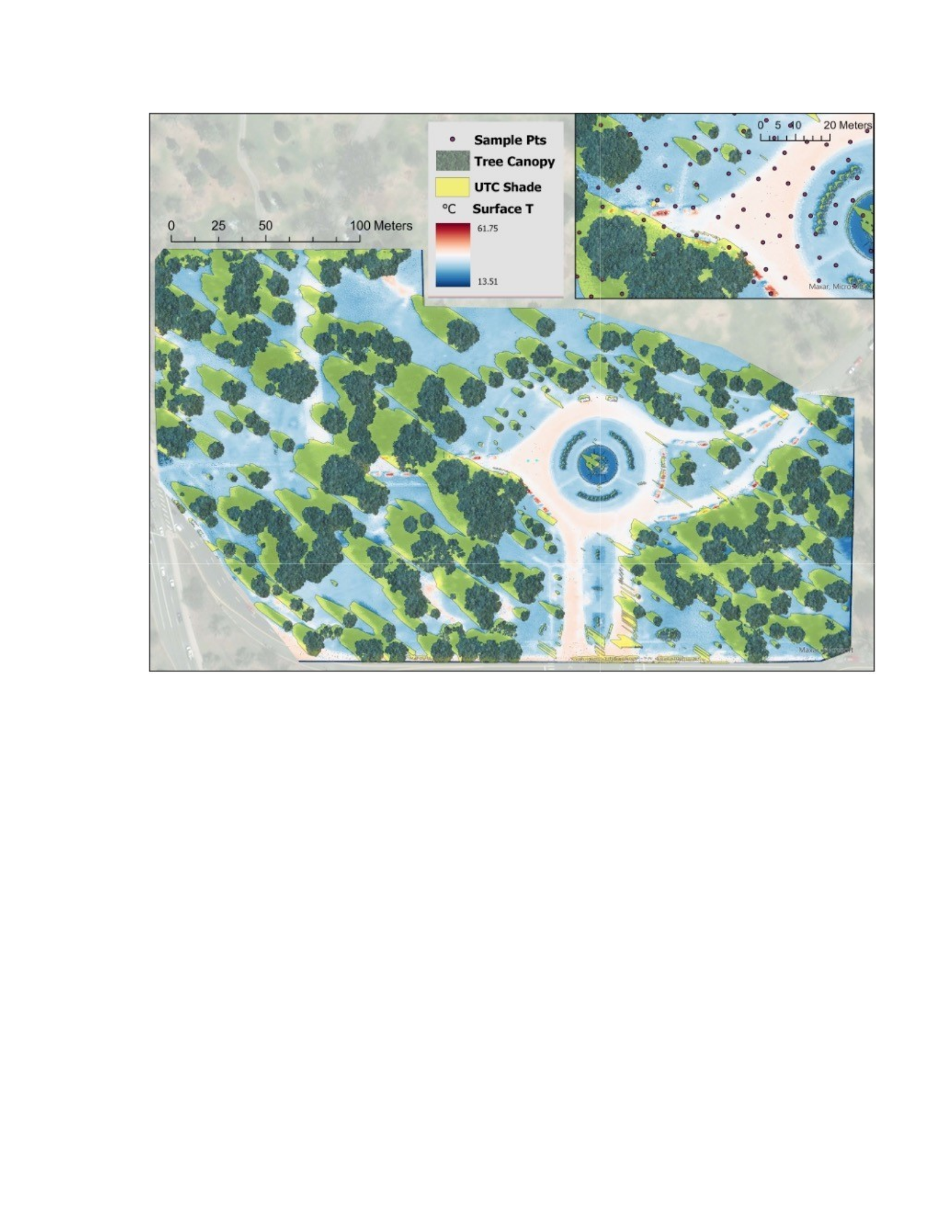
Figure 1: Denver City Park study area, with tree canopy derived from LiDAR, UTC
shade modeled from the tree canopy data, and the observed land surface temperature
in degrees Celsius collected with a thermal-multispectral sensor.
2D Land Cover Variable Creation
The surface cover for both the coarse-scale and fine-scale assessment was first
measured using pre-classified land cover data with a very high-resolution of 0.5 to 1
meter. For the CoarseScale assessment, these variables are subsequently aggregated as
areal metrics to the 30-meter resolution fishnet sample grid. This integrated dataset
effectively reflects the combined influence of land cover diversity and distribution
within the scope of a single sampled Landsat LST pixel. In contrast, the independent
predictors of surface temperature for the fine-scale assessment were coded as binary to

indicate presence of select physical attributes at a particular study area point location.
For instance, if UTC, turf, impervious surface, or UTC shade were present at a given
location, it received a value of “1” in the corresponding table cell, if absent a value of
“0”. A fourth numerical variable called “Near Distance” represented the Euclidean
distance in meters from a sampled point location to the closest tree crown polygon
feature. This variable was a proxy for the estimated effects of tree evapotranspirational
cooling. The integrated dataset effectively reflects the combined influence of land
cover diversity and distribution within the scope of a single sample point location.
Three distinct vector datasets were used in the classification of Denver’s 2D
land cover: 1) the 2020 Denver Tree Canopy dataset, produced by the University of
Colorado Denver with technical assistance from the University of Vermont Spatial
Analysis Lab for use by the Denver Department of Parks and Recreation, Forestry
Division was created using object-based image classification in conjunction with high
resolution color infra-red and LiDAR imagery to identify tree canopies
(https://denvergov.org/opendata/dataset/city - and - county - of - denver - tree - canopy 2020 );
2) The 2017 Comprehensive Citywide Impervious Surfaces dataset was created by the
City and County of Denver using two independent data sources, one digitized by
Denver’s
Public Works Wastewater Management Division and another by Kucera International
Inc.(https://www.denvergov.org/opendata/dataset/city - and - county - of - denver -
comprehensive citywide - impervious - surfaces ); and 3) The 2017 Denver Turf Grass
dataset, created using the prior two datasets and the 2008 orthorectified high-
resolution (6 inch/15 cm) aerial imagery available here
(https://www.denvergov.org/opendata/dataset/city - and - county - of - denver -

aerial imagery - 2008 ) . Again, object-oriented classification was used to identify all
pervious surfaces, then to delineate the turf grass from the other urban vegetation.
During UAS data postprocessing procedures, we evaluated the quality and
accuracy of the UAS data sets. The LiDAR data, acquired on July 16th, and the
thermal-multispectral imagery acquired on September 4th were of good quality. The
processing of the LiDAR data generated 3D point clouds, while multispectral
orthomosaics were created from the geometrically corrected spectral imagery. Object-
oriented analysis was conducted using Definiens Developer/ eCognition software to
map tree canopy and generate polygons of the individual tree crowns for the trees in
the City Park study area (Reda & Andreas, 2004). Definiens classifies objects based
on fuzzy logic rule sets. The software first segments raster surfaces into objects with
relatively homogeneous pixel values or value patterns. Objects are then classified
based on the distribution of values of pixels in the objects, the shape of objects, and
the spatial context of those shapes, including adjacency and overlap characteristics.
These UASderived tree polygons were used to map the UTC land cover for the fine-
scale assessment instead of the 2020 Denver Tree Canopy dataset. Reference Table 1
for a summary of the UAS mission data.
Table 1: UAS Missions
Date Location Site Operator Airframe Sensor Payload Data Products
7/16/19 Denver, CO Denver City
Park
USGS DJI Matrice
600
Yellowscan Mapper LiDAR,
Sony a600 Hi-Res RGB
LAZ/LAS point clouds,
Sfm DSM
9/4/19 Denver, CO Denver City
Park
USGS DJI Matrice
600
Micasense Altum 6-channel orthomosaic,
DEM /DSM/ nDSM

3D Shade Simulation and Shade Variable Creation
For the coarse-scale assessment, the three-dimensional (3D) properties of trees
used to model shade were obtained from publicly available 2017 FEMA LiDAR data.
The GIS software Quick Terrain Modeler 8.0 was used to differentiate and classify the
various surface features within the raw 3D LiDAR point cloud data, then convert this
information into raster elevation grids (Digital Elevation Models, DEM’s), 2D images
representing the top-down perspective of an area with distance measurements in the x,
y, and z dimensions. This initial process generated a bare earth DEM, and a Digital
Surface Model (DSM) depicting the bare ground with all surface features present,
including buildings, trees, cars, transmission lines, etc.
Alternatively, for the fine-scale assessment, the three-dimensional (3D)
properties of trees used to model shade were obtained from UAS-collected LiDAR
data acquired on July 16,
2019, under cloud-free conditions. Specifically, a DJI Matrice 600 hexacopter airframe
with the
Yellowscan Surveyor (equipped with Velodyne puck VLP-16) was flown between the
hours of 11 AM and 1 PM, when the sun was at its apex to optimize spectral
reflectance, maximize land surface temperatures, and minimize the effect of shadows.
The processing of the LiDAR data generated 3D point clouds. Definiens Developer/
eCognition software was used to differentiate and classify the various surface features
within the raw 3D LiDAR point cloud data, then convert this information into raster
elevation grids (Digital Elevation Models, DEM’s) including and a bare earth DEM,
and a Digital Surface Model (DSM) depicting the bare ground with all surface features
present, including buildings, trees, cars, transmission lines, etc.

ArcGIS Pro (10.5) was used for the remaining GIS processing. Polygons
representing the outlines of trees were used as intersection masks to extract 3D DSM
data for these objects, resulting in a partial DSM consisting only of trees. The isolated
and extracted trees for each dataset, were then fused (mosaicked) to a copy of its
respective bare ground DEM. For the Coarse-Scale assessment, the final product was a
DSM of the city of Denver consisting only of bare ground and its respective UTC,
with spatial resolution of 35.3 centimeters per pixel. For the fine-scale assessment, the
final product was a DSM of the Denver City Park study area consisting only of bare
ground and its respective UTC, with spatial resolution of 7.1 centimeters per pixel.
Tree shade was modeled based on the Sun’s spherical position (altitude and
azimuth) relative to the earth. A proven estimator of the Sun’s altitude and azimuth is
the Measurement and Instrument Data Center’s (MIDC) SPA Calculator, using the
Solar Position Algorithm
(SPA) developed by the National Renewable Energy Laboratory (NREL) (Reda &
Andreas, 2004; Levinson et al., 2009; Taylor, 2015). This SPA algorithm calculates the
solar zenith and azimuth angles in the period of the year -2000 to 6000, with
uncertainties of +/-0.0003 degrees based on the date, time, and location on Earth
(Reda and Andreas, 2004). These factors determine the position, duration, extent, and
intensity of the sun’s rays, and thus the shadows cast by the surface features at a
specific location.
The Hillshade tool in ArcGIS was used to simulate on-hour shadowing for a
particular location, on any day, for any given daylight hour or interval thereof. Several
studies have previously used the Hillshade tool to model shade, including Levinson et
al. (2009), Taylor (2015), and Yu et al. (2020). For the Coarse-Scale assessment, the

hourly altitude and azimuth data were generated by the SPA calculator for date of
August 4, 2017, which coincided with that of the Landsat 8 imagery used for the
coarse-scale LST. This process was performed seven times using the tree DSM as the
input 3D terrain feature for the coarse-scale assessment. This produced seven raster
grids representing the tree shadow coverage for each of the seven hours within the
diurnal interval from 11AM to 5PM. This interval was chosen to represent the portion
of the day with highest temperatures and with the greatest potential for UTC heat
mitigation (U.S. EPA, 2008; Meier & Scherer, 2012). For each hourly time step, a
pixel was assigned a value of 1 if shade was present and zero if it was not. Then the
seven, hourly shadow rasters for August 4, 2017, were combined into a single
composite image where the numerical values of individual pixels indicated the total
number of hours of tree shade that an area experienced during the 11am to 5pm
interval. In this case, because the composite shade map was developed for each pixel,
P = 1 in Eq. (1). The vector data layers representing the city’s municipal boundaries
and building footprints, were then used as intersection masks to classify and extract
the relevant agglomerations of shaded pixels, for their final compilation and
quantification.
The coarse-scale assessment used the metric Mean Shade-Hours to represent
the areal quantity of tree shade affecting the exposed horizontal surfaces of each city,
across time. To calculate the Mean Shade-Hours for a spatial area made up of j pixels
the following equation was used [Eq. (1)]:
𝑀𝑒𝑎𝑛𝑆ℎ𝑎𝑑𝑒 −
𝐻𝑜𝑢𝑟𝑠 = 𝜇!" = ∑"!#%$$! (1)

Where, i represents each hour step up to the total number of hours in the study, t, S is
the number of shaded pixels, and P is the total number of pixels in the surface extent
being estimated. The Zonal Statistics function was used to summarize number of
hours of shade falling on surface pixels by sampled grid cell, yielding a total sum and
mean of shade hours, where the latter equaled the sum of pixel shade hours divided by
the number of shaded surface pixels. Therefore, the effect from Mean Shade-Hours
differs in interpretation from turf and impervious areal measurements in that it
represents a unitless average. Instead, coefficients for Mean Shade-Hours represent a
marginal effect for the average 30-meter sample grid cell, which has 386 m2 of turf,
206 m2 of tree canopy, and 427 m2 of impervious surface.
Because the Mean Shade-Hours metric is calculated as function of time, it does
not solely represent area and is challenging to interpret. Thus, we also created two
mutually exclusive areal measures of shade. The metric Low Shade Area was used to
represent the total area occupied by pixels with one to four hours of tree shade. The
metric High Shade Area was used to represent the total area occupied by pixels with
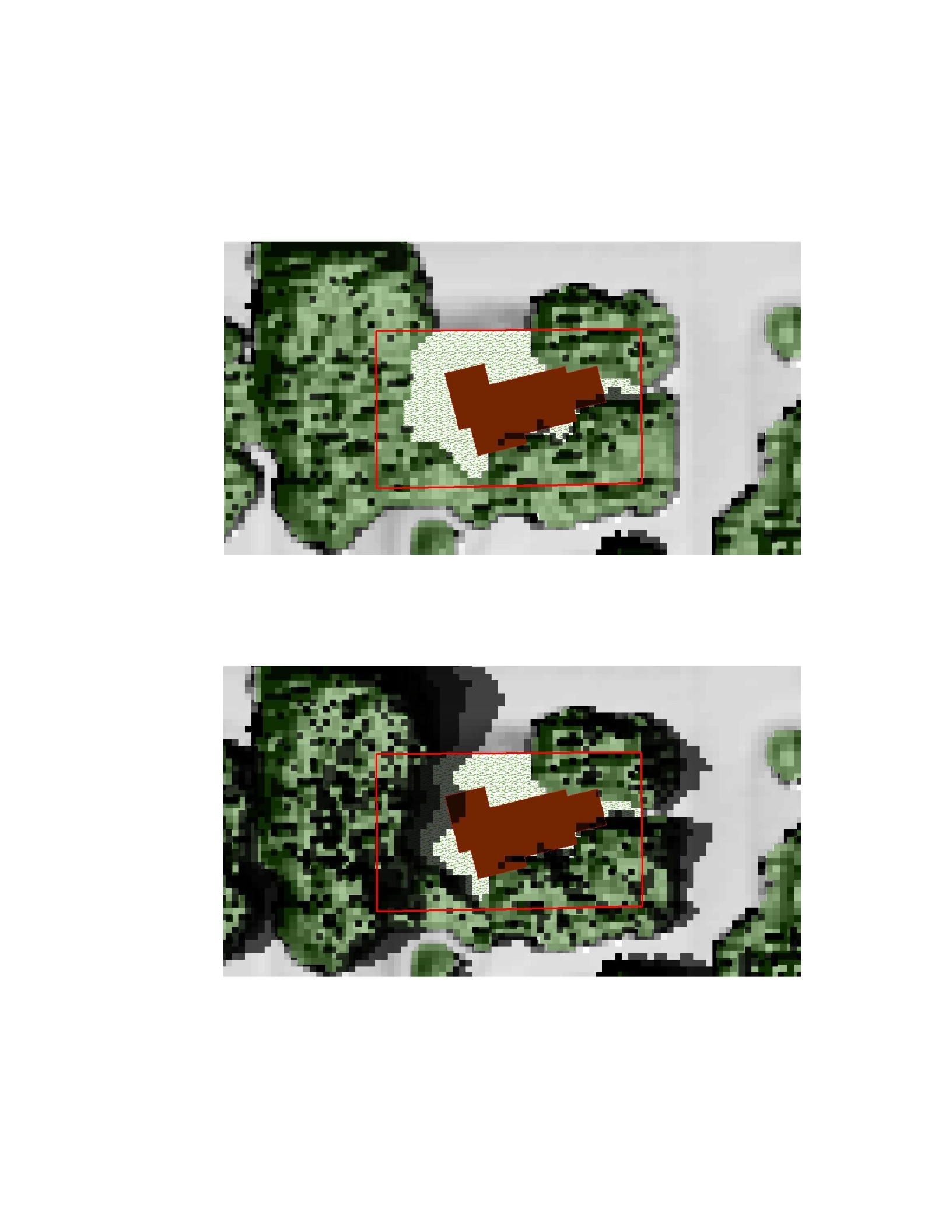
five to seven hours of shade. Reference Figure 2, for an example of course-scale
assessment simulated UTC shaded area for 12:00 PM and 3:00 PM.
For the fine-scale assessment, the hourly altitude and azimuth data were
generated by the SPA calculator for September 4, 2019, 9:30 AM, which coincided
with the date and start time for the collection of the UAS thermal-multispectral
imagery used for LST. The fine-scale assessment used the City Park trees only DSM
(7.1 cm/pixel) to simulate the single time-step of UTC shaded area using a simplified
version of the shade modeling methods described earlier for the coarse-scale
assessment. The areas of UTC Shade modeled for the 9:30 AM time-step were found
to be a near perfect match for the observed areal footprints of the shadows cast by City
Park trees in the natural color version of the UAS-collected thermal-multispectral
orthoimage.
12 PM Shade Area = 728 m2/1hr
13 PM Shade Area = 6455 m2/4hr

Figure 2: Coarse-Scale assessment, simulated UTC shaded areas
relative to UTC and a single-family home, modeled for the hours of
12:00 PM and 3:00 PM for Denver.
Statistical Methods
Coarse-Scale Assessment
We compared the ability of the UTC shade metrics (Mean Shade-Hours, Low
Shade Area, and High Shade Area), to explain variation in surface temperature in
relation to the commonly used UTC Area metric, at the relatively coarse spatial scale
of 30 meters. Initially, ordinary least squares (OLS) regression was used to test
different multivariable models, each with a unique combination of explanatory
variables. In addition to the UTC Area and UTC shade variables, the regressions
included control variables for impervious and turf grass surface area, which were also
key determinants of urban heat. Table 2 lists the variable definitions and sample
descriptive statistics for the coarse-scale assessment.
OLS regression was determined to be inappropriate for use given findings of
spatial autocorrelation in the error term (Moran’s I = 0.456, p-value < 0.00000),
reinforced by a significant Lagrange Multiplier test (robust LM [error] = 133587, p-
value < 0.00000). Instead, we used spatial error regression, which controls for
inflation of test statistics due to spatial autocorrelation, resulting in a more
conservative model that better avoids type 1 errors (Anselin,
1988; Anselin & Rey, 1991).
The VIF’s for Denver’s all-inclusive OLS regression model indicated moderate
multicollinearity for the explanatory variables Mean Shade-Hours (VIF = 5.50) and

UTC Area (VIF = 5.56), but not for Turf Area (VIF = 2.92) and Impervious Surface
(VIF = 2.90). Preceding regression analysis, Spearman’s rank order correlation was
used to measure the strength of association between all combinations of variable pairs.
The results indicated UTC Area was highly correlated with each of the shade variables
(Mean Shade-Hours, Low Shade Area, and
High Shade Area (Table 3). This collinearity between variable pairs prohibited the use
of model configurations that combined the use of both types of variables as predictors
within the same model. Ultimately, multimodal inference was used to determine
individual variable importance by comparing the predictive performance of different
models with differing variable configurations. Three spatial error models were run
with differing combinations of predictor variables, including one isolating the effects
of Low Shade and High Shade, also containing
Impervious Area and Turf Grass Area (Model 1); a second isolating the effects of
Mean ShadeHours also containing Impervious Area and Turf Grass Area (Model 2);
and a third isolating the effects of UTC Area, with Impervious Area and Turf Grass
Area (Model 3).
Table 2: Coarse-Scale Assessment Variable Descriptions
Variable Name Description Units Mean Std. Dev
Mean Surface
Temperature (μst)
the average of the thermal pixel
values, for a 30-m sample grid cell,
representing the mean day-time
surface temperature; derived from the
remotely sensed radiance detected by
NASA’s Landsat 8
°C 32.2 3.1
UTC Area the total surface area covered by
urban tree canopy crowns, for a 30-m
sample grid cell; derived from
municipal land cover data
m2 123.9 146.5

Impervious Area the total surface area covered by
impervious surfaces (buildings, roads,
driveways, sidewalks, parking lots),
for a 30-m sample grid cell; derived
from municipal land cover data
m2 429.7 263.1
Turf Grass Area the total surface area covered by turf
grass land cover with some shrub, for
a 30-m sample grid cell; derived
from municipal land cover data
m2 386.1 259.3
Mean Shade-Hours
Low Shade Area
High Shade Area
the total sum of pixel shade hours
divided by the number of shaded
surface pixels, for a 30-m sample
grid cell; derived from 3D LiDAR
data
the total surface area covered by
pixels with 1 to 4 hours of tree shade,
for a 30-m sample grid cell; derived
from 3D LiDAR data
the total surface area covered by
pixels with 5 to 7 hours of tree shade,
for 30-m sample grid cell; derived
from 3D LiDAR data
m2
m2
1.6
186.0
17.6
1.1
191.8
26.5
Table 3: Coarse-Scale Assessment Variable Correlations
Impervious
Area
UTC
Area
Mean
Shade-Hours
Turf
Area
Low
Shade Area
High
Shade Area
Mean Surface
Temperature
Impervious Area 1.00
UTC Area -0.13 1.00
Mean Shade-Hours -0.11 0.94 1.00
Turf Area -0.81 0.23 0.20 1.00
Low Shade Area -0.11 0.81 0.99 0.19 1.00
High Shade Area -0.11 0.91 0.94 0.20 0.90 1.00
Mean Surface Temperature 0.29 -0.32 -0.33 -0.34 -0.33 -0.32 1.00
Fine-scale Assessment
We then regressed observed land surface temperature sampled from within the Denver
City Park study area, against the chosen independent variables (Table 4) using
stepwise Ordinary Least Squares regression. No variable had a VIF in excess of 3.29,
with four out of the six terms under 2. The only variables with a VIF over 3 were those

for impervious surface and turf from the second OLS regression equation. A VIF value
of 4 is typically considered a key threshold for collinearity.
Table 4: Fine-Scale Assessment Variable Descriptions
Variable Name Description Unit Mean Std. Dev
Surface Temperature Observed surface temperature at sample. °C 28.100 5.672
Near Distance Distance from sample to the nearest tree. m 2.727 2.845
UTC Shade Presence of shade from trees (1/0) at sample. 0.405 0.491
Impervious Presence of impervious land cover (1/0) at sample. 0.220 0.415
UTC Presence of tree canopy land cover (1/0) at sample. 0.081 0.273
Turf Presence of turf land cover (1/0) at sample. 0.699 0.459
Next, the model was assessed for spatial autocorrelation. A distance-based
spatial weights matrix was created in GeoDa (Anselin, 2003) and the model was
assessed for spatial dependency with respect to that matrix. The resulting diagnostics
included a Moran’s I value of
0.2439 (p=0), indicates the presence of a moderate level of positive spatial
autocorrelation. This value suggests that there is a tendency for similar values to be
located near each other more than would be expected by chance, but the clustering is
not extremely strong. Next, we tested for lag versus error term dependency in the
model using Lagrange Multiplier tests (Anselin & Rey, 1991). The spatial error model
assumes that the error term is subject to autocorrelation due to omitted variable bias,
while the spatial lag model assumes that there is systematic autocorrelation due to
spillovers in the dependent variable (Anselin, 1988). Lagrange Multiplier and Robust
Lagrange Multiplier test were all significant, but test statistics were much higher for

the Lagrange tests on lag (Robust LM lag= 70.3, p=0; Robust LM error= 11. P=0),
indicating the need to model spatial lag.
There are several forms of spatial lag regression from which to choose. The
most common is the Simultaneous Autoregressive (SAR) model (Eq. 2), which
assumes the existence of spillover effects in the dependent variable such that the value
of yi influences yj which in turn influences yk and so on, with the result that a marginal
change in the observational unit can have a cascading impact on the outcome variable
in all other observational units.
y = ρWy + Xβ + ε (2)
Where y= land surface temperature, ρ= spatial lag parameter, W= weights
matrix, X=matrix of observations of the independent variables, β= vector of
coefficients and ε is the error term.
The use of SAR requires a plausible underlying mechanism for spatial
spillovers in the dependent variable. In this case, we hypothesize that it is likely due to
misclassified instances of land cover type among the independent variables
representing different surface cover.
While SAR does not explicitly model the direct impact on the dependent
variable in observation i of independent variables for i’s neighbors, as the so-called
“Spatially Lagged X” (SLX) and “Spatial Durbin” models do, it does account for
neighboring independent variable impacts indirectly, as those variables influence the
dependent variable of the neighbors, which in turn influence the dependent in the
observation in question. This fact means that regression coefficients in SAR are not
interpreted in the same way as those in ordinary least squares (OLS) regression.
Rather, a special table of spatial spillover impact effects is needed to interpret the

coefficients’ so-called direct, indirect, and total effects. The first of these represents the
marginal effect of each x on y within a given spatial observation, i; the second
represents the effect on y at observation i of changing x in i’s neighbors; and the third
represents the average global effect due to a change in x across all observations
simultaneously (LeSage, 2008, 2014; J. LeSage & Pace, 2009).
OLS and SAR regressions were conducted in R 4.2.1 using the LAGSARLM
function.
Spatial data operations in R required the use of the spatialreg, rgeos, rgdal, and spdep
packages. Weights were imported into R from GeoDa using the read.gal function.
Given the large matrix weights, the use of a “sparse trace matrix” of weights was
required in order to generate the “impacts” table. We conducted regressions where the
effects of both UTC and turf land cover variables were modeled (and omitted as
control variables) separately in two different equations. Additionally, while it was not
possible to include the spatially correlated UTC and tree shade variables in the same
models for the Coarse-Scale assessment, this was a possibility for the finescale
assessment. This was due to the application of SAR models that account for spatial
dependence directly. That is, the collinearity could be a byproduct of the spatial
process itself, rather than an issue with the variables per se. Further, the SAR model's
structure can handle more complexity since the spatial correlation is explicitly
modeled. This can reduce the problems associated with multicollinearity. Finally, the
spatial lag of the dependent variable can help to stabilize the variance and reduce the
multicollinearity impact on coefficient estimates.

Nonetheless, including variables that are perfectly collinear would still be problematic.
Consequently, it is still important to examine the variables for collinearity and
understand how they are related to each other and to the spatial structure of the data.

RESULTS
Coarse-Scale Assessment
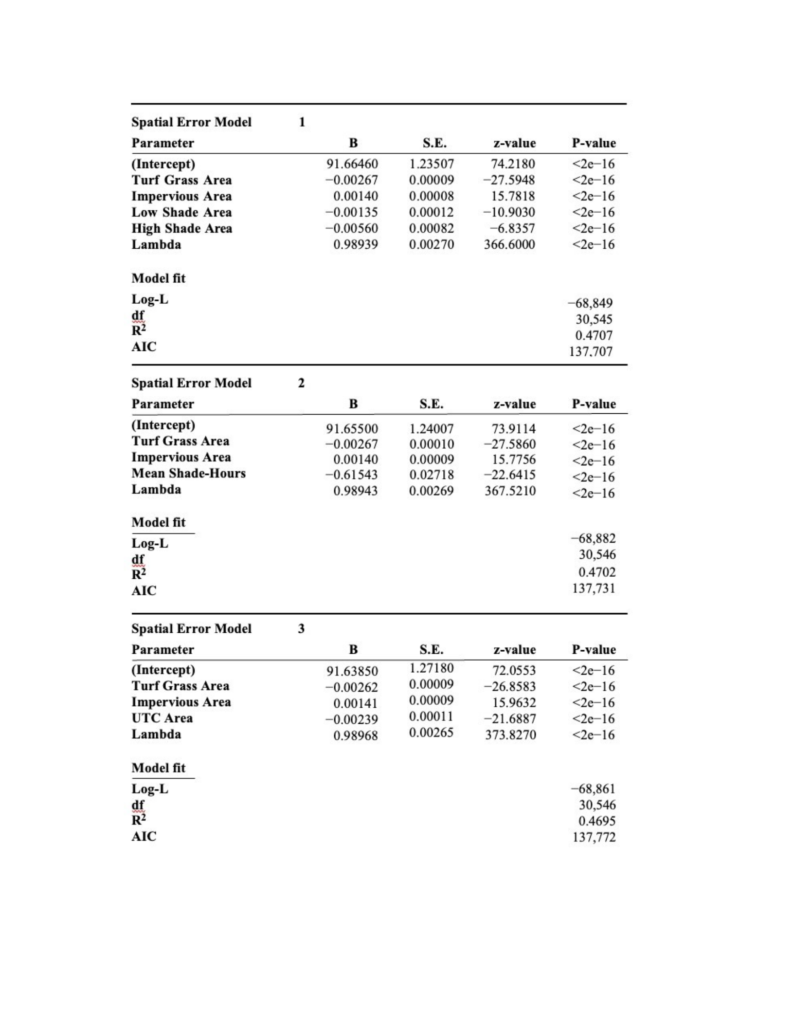
The Spatial Error Regressions indicate that in Denver, Impervious Area had a
positive relationship with the dependent variable for LST, Mean Surface Temperature
(Table 5). The remaining variables, UTC Area, Turf Grass Area, Mean Shade-Hours,
Low Shade Area (<=4 hours), and High Shade Area (>=5 hours), demonstrated a
negative relationship with Mean Surface Temperature (Table 5). All variables in all
models were significant at the 99% confidence level. Because data were
untransformed, each coefficient represents the marginal increase or decrease in
degrees Celsius of surface temperature associated with a one squaremeter increase in
the area of that variable.
Model 1 assessed the effects of the High- and Low-Shade Area variables by
including the two predictors in the same model, along with Turf Grass and Impervious
Area. Recall, that the collinearity between UTC Area and all UTC shade variable pairs
prohibited the use of model configurations that combined the use of both types of
variables as predictors within the same model. The coefficient of High Shade Area was
the largest in magnitude for Model 1, indicating that a single square meter of High
Shade Area more than offset the effect from a single square meter of impervious
surface, but one square meter of Low Shade Area did not. High Shade Area resulted in
a net decrease to mean surface temperature of -17.8 °C ( -0.0056 °F). Additionally, a
single square-meter increase in Turf Grass Area offset that of Impervious Area.
Finally, Low Shade Area offsets 72% of Impervious Area’s effect, and High Shade
Area offsets 260% of Impervious Area’s effects in Denver. The pseudo R2 value for

Model 1 (0.4707) was the largest, indicating that it explained the most variance in LST
with 47.1%.
Model 2 assessed the effects of the Mean Shade-Hours variable, in addition to
Turf Grass and Impervious Area. Once again, the UTC Area metric was excluded from
the model due to collinearity with UTC shade variables. The coefficient of Mean
Shade-Hours (-0.615) was the largest by several orders of magnitude, compared to
Turf Grass (-0.00267) and Impervious (0.0014). However, Mean Shade-Hours is a less
interpretable variable, since it represents a sum of areas averaged across the time they
are shaded. This contrasts with the other explanatory variables, which represent area
only. Still, the pseudo R2 value for Model 2 (0.4702) was the second largest, indicating
that it explained 47.0% of the variance in LST.
Model 3 assessed the effects of the UTC Area variable, in addition to Turf
Grass and Impervious Area. Like shade, the effect of UTC Area offset that of
Impervious Area. By comparison an equivalent unit of UTC Area offsets 60% of
Impervious. A comparison of Model 3 with Model 1 using AIC, indicate the model
with High Shade Area and Low Shade Area variables but no UTC Area variable
(Model 1), outperformed the model with UTC Area but no shade area variables
(Model 3) in Denver (AIC= 137707 for 1, and 137772 for 3). The lower AIC score for
Model 1 suggests that even though the model’s AIC is penalized for having one more
variable than Model 3 (i.e. the former has variables for High Shade Area and Low
Shade Area while the latter only has UTC Area), the increase in model fit more than
makes up for the loss in model parsimony (Akaike, 1978, 1979; Burnham &
Anderson, 2003).

The comparison of Model 2 with Model 3 reinforces this message. The model
with Mean Shade-Hours (2) had more support (lower AIC) than the model with UTC
Area (3) and no shade variable. Ultimately, the model comparisons indicate that shade
variables had more support than the model with just UTC Area alone, and that the
model with two shade area variables performed
better than an averaged shade metric.
Table 5: Coarse-Scale Assessment Spatial Error Regression Results.

Fine-scale Assessment
Summary statistics of all Fine-scale Assessment variables are presented in
Table 4. The rsquared of the OLS model was 0.584, with 995 degrees of freedom
(Table 6). The SAR models had a pseudo R2 of 0.666 (Table 7). All variables for the
OLS (Table 6) were significant at the 99 % confidence level and of the expected sign.
Similarly, all variables for the SAR (Table 7) models were significant at the 99.9 %
confidence level, and of the expected sign. The SAR models (SAR 1 and SAR 2) were
each specified with an OLS equation (OLS 1 and OLS 2) as its basis, adjusting for
spatial dependencies through a lagged variable approach. The residuals of the model
ranged from -11.91 to 17.83, with a median close to zero (-0.20408), indicating a
symmetric distribution of residuals around the median value. However, the presence of
significant outliers, as evidenced by the minimum and maximum values, points to
potential heteroscedasticity or non-linearities not captured by the model.
The model identified significant spatial autocorrelation, as evidenced by the
rho parameter (ρ = 0.4148), which measures the strength of the relationship between a
location and its neighbors. The likelihood ratio (LR) test, Wald statistic, and associated
p-values (< 2.22e-16) strongly rejected the null hypothesis of no spatial
autocorrelation, affirming the necessity of the SAR model approach. The Akaike
Information Criterion (AIC) for the SAR model was 5259, compared to 5438 for a
standard linear model (lm), suggesting a better fit to the data. The Lagrange Multiplier
(LM) test for residual autocorrelation yielded a test value of 0.03034 with a p-value of
0.86172, indicating no significant residual spatial autocorrelation, thus affirming the
adequacy of the spatial lag model in capturing spatial dependencies.

The model estimated the effects of several predictors, including Near Distance,
UTC
Shade, Impervious, Turf, and UTC on the outcome variable Surface Temperature. The
coefficients and their asymptotic standard errors were reported, alongside z-values and
p-values to assess statistical significance. The Intercept showed a highly significant
positive effect (Estimate = 17.178142, p < 2.2e-16), indicating the baseline level of the
outcome variable when all predictors are zero. Near Distance had a positive and
statistically significant impact (Estimate = 0.133120, p = 0.0004088), suggesting that
Surface Temperature values tend to decrease with proximity to UTC. This relationship
supports the use of Near Distance to model the cooling effects of tree
evapotranspiration. UTC Shade exhibited a strong negative effect (Estimate = -
5.454411, p < 2.2e-16), indicating that higher values are associated with a decrease in
Surface Temperature. Impervious showed a significant positive effect (Estimate =
4.348633, p < 2.2e-16), suggesting that it contributes positively to the outcome
variable. UTC also had a slightly positive and significant effect (Estimate = 1.735797,
p = 0.00001784) on Surface Temperature, which contradicts the results documented
by the preponderance of previous research. That said, this result appears to be
indicative of the elevated surface temperatures associated with the tops of tree crowns
at some randomly sampled locations.
In a second configuration of SAR model (SAR 2), the UTC variable was
replaced by Turf, which exhibited an equivalent, but negative effect (Estimate = -
1.735797, p = 0.00001784), indicating that higher areal quantities of turf are
associated with a decrease in Surface

Temperature. This change in the model’s predictors caused a reduction in the effect
size of Impervious (Estimate = 4.348633, p = 2.9e-8). All other values in SAR 2
remained relatively unchanged. Ultimately, tree shade is easily the most influential
variable implemented for the fine-scale assessment. Results show that at fine-scale,
UTC Shade is inversely correlated with heat and highly significant, while UTC is
positively correlated with heat and much less significant, demonstrating that tree shade
is clearly the best predictor of heat mitigation which has historically been associated
with the presence of trees.
A comprehensive analysis of the impacts of SAR models, focused on the
direct, indirect, and total effects of predictor variables on Surface Temperature,
providing insights into how each variable influences the outcome both locally (direct)
and through spatial spillover effects (indirect) (Table 8). Near Distance showed a
positive direct impact (0.138) and a positive indirect impact (0.08942), leading to a
total impact of 0.2275. This indicates that proximity to UTC positively affects the
outcome variable, both directly and indirectly through spatial spillovers. UTC Shade
exhibited significant negative impacts across all measures: direct (-5.656), indirect (-
3.66378), and total (-9.3202). The higher values are associated with a substantial
decrease in Surface Temperature highlighting the negative influence of this variable at
both local and broader spatial scales. Impervious had a strong positive direct impact
(4.510), a positive indirect impact (2.92102), and a total impact of 7.4307, reinforcing
the importance of considering impervious surface measures in spatial analyses. UTC
demonstrated positive effects: direct (1.800), indirect (1.16595), and total (2.9660
suggesting increased tree coverage increased the outcome.

Near Distance showed the lowest standard errors, suggesting high precision in its
impact.
estimates. Conversely, UTC had the highest standard errors, indicating less precision
in its impact estimates. Z-values provided a measure of statistical significance for each
impact. All variables showed significant z-values across direct, indirect, and total
impacts, indicating strong evidence against the null hypothesis of no impact. P-values
confirmed the statistical significance of the impacts, with all variables showing p-
values well below the conventional threshold of
0.05. Notably, UTC Shade and Impervious exhibited extremely low p-values across all
impact measures, indicating a very high level of statistical significance.
The UAS thermal-multispectral orthoimagery used for the fine-scale
assessment allowed for the direct valuation and comparison of the sampled surface
temperature values between shaded and unshaded impervious and turf grass surfaces.
The descriptive statistics for these results are summarized in Table 9, where the mean
surface temperature cooling effects of shaded and unshaded impervious and turf grass
surfaces were 6.8 °C and 6.7 °C, respectively. The findings underscore the complexity
of microclimatic spatial relationships and corroborate the importance UTC shade
effects in the mitigation urban surface temperatures. The statistical significance of
these impacts, supported by simulation results, provides robust evidence for the
influential role of UTC shade metrics as vital tools for guiding policymaking, urban
planning, and environmental management.
Table 6: Fine-Scale Assessment OLS Regression Results

Table 7: Fine-Scale
Assessment SAR Results
SAR 1
Estimate Std. Error z value Pr(>|z|) Sig
Intercept 17.178 0.844 20.351 0.00000 ***
Near Distance 0.133 0.038 3.534 0.00041 **
UTC Shade -5.454 0.238 -22.920 0.00000 ***
Impervious 4.349 0.275 15.789 0.00000 ***
UTC 1.736 0.405 4.290 0.00002 **
SAR 2
Estimate Std. Error z value Pr(>|z|) Sig
Intercept 18.914 0.896 21.104 0.00000 ***
0.00041 **
Near Distance 0.133 0.038 3.534
UTC Shade -5.454 0.238 -22.920 0.00000 ***
0.00000 ***
Impervious 2.613 0.471 5.545
Turf -1.736 0.405 -4.290 0.00002 **
Signif. codes: ‘***’ 0.001 ‘**’ 0.01 ‘*’ 0.05
Rho: 0.4148, LR test value: 181.2
Pseudo R-squared: 0.6664
z-value: 14.55, p-value: < 2.22e-16
Wald statistic: 211.8, p-value: < 2.22e-16
ML residual variance (sigma squared): 10.73, (sigma: 3.276)
AIC: 5259, (AIC for lm:5438)
LM test for residual autocorrelation: 0.030, p-value: 0.8617
OLS 1
Coefficient Std. Error T stat P-value Sig
Intercept 29.070 0.214 135.680 0.00000 ***
Near Distance 0.114 0.042 2.710 0.00680 **
UTC Shade -6.596 0.248 -26.620 0.00000 ***
Impervious 5.828 0.286 20.400 0.00000 ***
UTC 1.282 0.451 2.840 0.00450 **
OLS 2
Coefficient Std. Error T stat P value Sig
Intercept 30.352 0.458 66.270 0.00000
0.00680
***
**
Near Distance 0.114 0.042 2.710
UTC Shade -6.596 0.248 -26.620 0.00000
0.00000
***
***
Impervious 4.546 0.507 8.970
Turf -1.282 0.451 -2.840 0.00450 **
Signif. codes: ‘***’ 0.001 ‘**’ 0.01 ‘*’ 0.05
Residual standard error: 3.66 on 995 degrees of freedom
Multiple R-squared: 0.586, Adjusted R-squared: 0.584
F-statistic: 352 on 4 and 995 DF, p-value: <2e-16

Table 8: Fine-Scale Assessment SAR Results of Direct, Indirect, & Total
Impacts
SAR 1 Impacts
Direct Indirect Total P-Direct P-Indirect P-Total
Near Distance
UTC Shade
Impervious
Tree
0.138
-5.656
4.510
1.800
0.089
-3.664
2.921
1.166
0.228
-9.320
7.431
2.966
0.00054
0.00000
0.00000
0.00004
0.00160
0.00000
0.00000
0.00030
0.00068
0.00000
0.00000
0.00006
SAR 2 Impacts
Direct Indirect Total P-Direct P-Indirect P-Total
Near Distance
UTC Shade
Impervious
Turf
0.138
-5.656
2.710
-1.800
0.089
-3.664
1.755
-1.166
0.228
-9.320
4.465
-2.966
0.00056
0.00000
0.00000
0.00001
0.00170
0.00000
0.00000
0.00009
0.00075
0.00000
0.00000
0.00001
Signif. codes: ‘***’ 0.001 ‘**’ 0.01 ‘*’ 0.05
Table 9: Fine-Scale Assessment Land Surface Temperature – Shaded Versus
Unshaded
Sample Surface
Conditions
Count Mean
LST (°C)
Std.
Dev
Min
(°C)
Max
(°C)
Range
(°C)
Shaded Impervious 53 28.52 6.014 19.17 42.4 23.26
Unshaded Impervious 167 35.299 4.964 19.74 49.4 29.68
Shaded Turf Grass 284 22.735 3.548 16.16 42.2 26.06
Unshaded Turf Grass 415 29.438 2.755 19.94 48.2 28.29

DISCUSSION
The Urban Heat Island (UHI) effect is when a city’s urban core experiences
higher temperatures than outlying rural areas due to factors like building density and
the replacement of natural vegetation with heat-absorbing materials like concrete and
asphalt. These dense urban areas that are much warmer than their surroundings —
have grown in area, number, and intensity, with Denver emerging as one of the
nation’s most “impervious” cities. In the most impervious parts of Denver, summer
temperatures are 12 degrees hotter than in older neighborhoods with more trees and
lawns, which do not radiate as much heat. Denver’s overall UTC coverage for the
entire city is 13%, among the lowest in ranked cities nationwide, with a Downtown
UTC coverage of just 3%. Increasing vegetation as a strategy for mitigating urban heat
has become a key component of Denver planning policy. Recently, city crews have
been planting about 6,700 trees a year (mostly oak, elms and Kentucky coffee trees),
achieving survival rates as high as 90%. Their goal is to expand Denver’s overall tree
canopy, from 13% of the city, to 20%.
Research demonstrates that the presence of urban greenspace does influence
air and surface temperatures (Yokohari et al., 1994; J. Zhang & Wang, 2008; K.
Zhang et al., 2009; Y. Liu et al., 2017). Street trees were shown to have a significant
benefit, with reductions between
0.5 °C and 1.8 °C when canopy coverage is increased from 10% to 55% (Wang &
Akbari, 2014, 2016). While the inverse relationship between vegetation fraction and
LST is well documented

(Weng et al., 2004; Chen et al., 2006; Yuan & Bauer, 2007; S. Li et al., 2010; W. Li et
al., 2017; Y. Liu et al., 2017), the impacts of tree shade on the urban thermal
environment at various geographic scales is less thoroughly characterized. Dense
shade can lower energy consumption for cooling by up to 49%, but most studies have
been conducted at small scales and do not account for the varying impacts of different
types of vegetation or their interactions with urban infrastructure.
This research supports the idea that a more nuanced approach to urban
greening is necessary. Simply planting more trees may not be sufficient for effective
heat mitigation in urban areas. Urban planners should focus on strategic shade
placement through shade modeling, considering the three-dimensional spaciotemporal
patterns of shade. This highlights the importance of tree shade distribution in urban
planning. It suggests that the two-dimensional metric of Urban Tree Canopy (UTC)
coverage is inadequate as it doesn't capture the threedimensional distribution of shade
and its dynamic nature with the sun's movement. There is a need for very high-
resolution (pixel area <= 1m) spatial data to accurately map, measure, and compare the
impact of UTC and UTC shade on urban LST, and cities could leverage modern
remote sensing techniques using LiDAR and thermal infrared imagery for this
purpose.
Understanding the specific heat reduction performance of different types of land cover
and shade variables can lead to more targeted and effective UHI mitigation strategies.
This research consists of two separate investigations conducted at different
spatial scales: 1) a Coarse-Scale assessment, and 2) a fine-scale assessment. In the
Coarse-Scale assessment, we introduce new methods for modeling and evaluating
hourly UTC shade at a local spatial scale of 30 meters, for an entire city, and compare

the heat predicting performance of the UTC shade metrics to that of UTC coverage.
This portion of the analysis relied solely on remote sensing data collected by
conventional means (i.e. manned-aerial surveys and earth-observing satellites). The
results of the associated spatial error regressions show that UTC shade is valuable in
predicting differences in surface temperature and delivers information in its signal that
is not contained in the UTC coverage variable. While the models with UTC shade
variables consistently outperform those with UTC coverage based on AIC multi-
coarse-scale assessment model comparison, the new information revealed by tree
shade variables is quite limited, due to the high degree of spatial correlation between
UTC and its projected shade effects at a 30-meter scale. Further, models show that the
effect size (regression coefficients) of the High Shade Area variable was larger than
the UTC Area variable, while that of the Low Shade Area variable was slightly smaller.
Also, the pseudo-R2 values in Table 5 indicate that our shade variables for the provided
only a minor improvement in overall model fit.
In the fine-scale assessment, the analysis methods were applied to a very high-
resolution dataset acquired with UAS and used to model and evaluate hourly UTC
shade at a microscale of
41 centimeters, to compare the heat predicting performance of the UTC shade metric
to that of
UTC coverage. The imagery was collected using the Altum Multispectral
Sensor from MicaSense, which provided thermal imaging powered by FLIR (forward-
looking infrared), and hi-res multispectral ortho-images in red, green, blue, red edge,
and near-infrared spectrums. The finer spatial resolution of the UAS data dramatically
improved both the accuracy and precision of the simulated tree shade and its

explanation of the variance in LST. The added capability of collecting hi-res
thermographic imagery significantly enhanced this phase of analysis, enabling
researchers to measure the temperature of surveyed surfaces directly. At this finer
spatial scale of analysis there was a distinct, visible, and quantifiable difference in the
thermal effect of the areas affected by UTC shade, compared with standard UTC
coverage (Table 7). Shade was shown to reduce mean temperatures by 6.78 °C across
all impervious surfaces and by 6.70 °C across all turf surfaces of the sampled data,
when compared to their unshaded counterparts (Table 9). The validity of the measured
thermal impact of tree shade effects is supported by the statistical rigor of the results
from the SAR models implemented in this fine-scale phase of analysis. The results of
the SAR models confirmed the superior power and heat mitigating impact of tree
shade represented by the UTC Shade variable, versus the effects of
evapotranspirational cooling (Upmanis et al., 1998) embodied by the Near Distance
and UTC variables (Table 7). Although, tree shade effects are measured for the
specific date and time of September 4, 2019, at 9:30 AM, it is indicative of the
potential heat mitigating microclimatic impacts experienced in Denver from tree shade
during the warmer summer months.
We believe this research demonstrates the value and feasibility of explicitly
mapping urban tree shade. Not only is heat mitigation a critical function of urban
trees, and one that this is imperfectly represented by UTC coverage measures, but the
methods and data needed to map shade are more accessible than ever. Given the
importance of urban heat as a public health and environmental justice issue (Flocks et
al., 2011), tools like this will play an increasingly important role in helping to identify
critical gaps in shade coverage from unshaded residential buildings, to major

pedestrian routes, outdoor gathering places, and safe routes to schools. That
information can in turn be used to target new green investments. The need for such
tools and approaches will only grow as climate change exacerbates the urban heat
island effect (Solecki et al., 2005, 2015). Meanwhile, advances in GIS data procedures
and computational power will make the automation and routinization of shade
mapping more easily replicable in the future.
Nonetheless, this methodology does entail some limitations. One is that we
measure heat using surface, and not air temperature, which would require extensive in
situ monitoring data. Further, the surface temperature associated with UTC crowns is
from the exposed upper portions of the UTC, as opposed to the surfaces below. We
acknowledge the limitations associated with the use of such data, but feel it is the best
representation of urban temperatures, in lieu of highresolution atmospheric
temperature data which does not yet exist. Ideally, such a study would be based on
atmospheric data, but conducting such an analysis would require a massive data
acquisition effort to measure atmospheric temperatures.

CONCLUSION
This paper presents a new methodology for modeling urban tree canopy shade
effects, as an augmentation to normal UTC Assessments. The method is then applied
to the analysis of the city Denver, Colorado – at two spatial scales of analysis, 30
meters and 41 centimeters. Unlike the generic approach of conventional UTC
assessments, a tree shade inventory incorporates additional data informing on the
dynamic spaciotemporal fluctuations in the daily microclimates of an urban area.
This research demonstrates that UTC shade mapping provides valuable
information that is not conveyed by traditional UTC coverage. This is not to say that
shade inventories should replace UTC assessments, but rather that the former should
augment the latter in cases where managers are seeking to characterize urban heat and
plan for heat mitigation. Numerous urban heat studies have focused on UTC coverage
as a key variable for predicting reductions in urban LST (Aniello et al., 1995; Hart &
Sailor, 2009; Loughner et al., 2012), yet analyses using UTC shade coverage as a
predictor of urban LST are much fewer in number. This study finds that UTC Shade is
a better predictor of LST than UTC area at scales less than or equal to 1 meter,
suggesting that more research is needed on shade as a management metric.
Nonetheless, it is increasingly clear that shade mapping can be used as a valuable tool
in prioritizing sites for new heat mitigating grey and green solutions.

