


INTRODUCTION Climate change has long been expected
Main Text
Climate change has long been expected to carry wide-ranging ecological impacts (Clark
1988; Graham and Grimm 1990; Harvell, Mitchell et al. 2002; Walther, Post et al. 2002). As
temperatures warm, species are expected to respond by advancing their phenology, or the timing
of seasonal activities, to be earlier in the year (Parmesan and Yohe 2003; Root, Price et al. 2003;
While and Uller 2014; Thackeray, Henrys et al. 2016). Species are expected to shift their
geographic ranges as conditions become less suitable in their native ranges and more suitable at
higher latitudes and elevations, which may allow non-native species to flourish (Parmesan,
Ryrholm et al. 1999; Chen, Hill et al. 2011). In accordance with Bergmann’s rule, species should
evolve smaller body sizes under warmer conditions, thus increasing their surface area to volume
ratios and promoting heat loss (Gardner, Peters et al. 2011). Sea level rise and the expansion of
deserts will exacerbate existing habitat loss experienced by many species (Thomas, Cameron et al.
2004; Mac Nally, Bennett et al. 2009). Finally, warming temperatures and increasing temperature
variability may impact temperature-dependent host-parasite interactions (Harvell, Mitchell et al.
2002; Jones, Patel et al. 2008; Rohr and Raffel 2010).
Although it is widely agreed that climate change will impact ecosystems and wildlife, there
are many controversies concerning how ecological processes will be altered over the coming
decades. For example, researchers have debated which species are more likely to experience
phenological or range shifts (Thuiller 2004; Visser and Both 2005; Parmesan 2007; Morin and
Thuiller 2009). There has also been extensive debate over whether infectious disease prevalence

is likely to increase or remain constant with climate change (Lafferty 2009; Rohr, Dobson et al.
2011; Altizer, Ostfeld et al. 2013). The reason for these controversies may be that climate change
is impacting diverse processes across a wide range of spatial, temporal, and allometric scales. The
interplay between fine-scale processes and broad scale dynamics can often generate large and
unpredictable changes to ecosystems (Wiens 1989; Levin 1992). Science currently lacks predictive
frameworks for which species are more likely to be impacted by climate change across scales.
A decades-old hypothesis in ecology suggests that biotic processes, such as predator-prey
or host-parasite interactions, should control species distributions at small, local spatial scales;
meanwhile, abiotic factors, such as climate or elevation, should drive distributions at large, regional
scales (Fig. 1.1) (Menge and Sutherland 1976; Wiens 1989; Levin 1992). Therefore, single-scale
studies may find different processes controlling species distributions if they are conducted at
different spatial scales. Cross-scale studies can produce elevation-richness curves that are either
linear or hump-shaped depending on the focal scale (Rahbek 2005), give contrasting richness-
productivity relationships (Chase and Leibold 2002), alter the perceived importance of competition
and predation on biodiversity (Menge and Sutherland 1976), and change the factors found to
influence community assembly (Trisos and Petchey 2014). In addition, studies at incorrect spatial
scales have been shown to bias estimates of thermal tolerance in plants (Trivedi, Berry et al. 2008)
or estimates of climate impacts on crop yields (Mearns, Easterling et al. 2001), parameters that are
especially important to measure accurately with increasing climate change. Phenological studies
at small spatial scales have been used to extrapolate large-scale regional patterns even in different
climates (e.g., Rosenzweig, Karoly et al. 2008; While and Uller 2014), which may be problematic
if phenological shifts are driven by different climatic processes in different regions. On the other
hand, continental and even global-scale climate data has been used to explain extinctions of
Atelopus species linked to disease, even though these species generally occur in small and
climatically unique ranges (Fig. 1.2) (Pounds, Bustamante et al. 2006; Rohr and Raffel 2010).

Because climate change is occurring heterogeneously in space (Pachauri, Allen et al. 2014), it is
critical to analyze fine-scale responses to climate change using appropriate finescale data.
It is also likely that climate change impacts may vary as a function of temporal scales.
Climate change projections indicate that a global mean temperature increase of 2-4°C is taking
place on the order of decades, a much faster transition than previous climate change throughout
Earth’s history (Pachauri, Allen et al. 2014). In addition, climate change is expected to increase
variability in temperature on short time scales on the order of days or weeks (Easterling, Meehl et
al. 2000; Yeh, Kug et al. 2009). Therefore, species will vary in their ability to adapt to climate
change depending on not only their ability to adapt to mutli-decadal shifts in mean temperature,
but also how well they acclimate to increasing variation in temperature; in other words, they will
have to adapt to change across different temporal scales. Small organisms generally have a faster
pace of life with shorter generation times than large organisms (Blueweiss, Fox et al. 1978), and
thus will have greater opportunities to evolve and adapt to changing conditions. Recent evidence
also suggests that small organisms are more capable at acclimating to short-term temperature shifts.
When given short (≤1 day) acclimation times, small organisms demonstrate a strong relationship
between acclimation temperature and optimal performance temperature, while large organisms do
not (Fig. 1.3) (Rohr, Civitello et al. in review), suggesting that smaller organisms acclimate faster
than large organisms, possibly because they have fewer cells and processes to adjust (Gillooly,
Brown et al. 2001).
Thus, I hypothesize that an understanding of how climate change is occurring across
temporal scales can inform our understanding of climate change impacts across allometric scales.
For example, it’s likely that small organisms track their phenology more closely to increasing
temperatures than large organisms if they can acclimate to those temperatures quicker. Parasites
may also acclimate to temperature shifts faster than hosts because parasites are almost always
smaller than hosts, and thus have fewer metabolic processes to adjust during acclimation. This

could cause parasites to gain a brief but significant advantage in host–parasite interactions when
conditions are variable (Fig. 1.4) (Raffel, Romansic et al. 2013). In addition, the Baas Becking
hypothesis states that small organisms have wider thermal breadths, or temperature ranges where
performance is relatively strong, than large organisms (Baas-Becking 1934). This could cause hosts
to face performance gaps with parasites at temperatures far from those where parasite performance
peaks (Fig. 1.5). For cold-adapted hosts and parasites, the gap may be likely to occur at warmer
temperatures, because cold-adapted parasites with broad breaths are more likely to be limited by
extreme cool conditions than moderate, warmer conditions. Similarly, warm-adapted hosts may be
vulnerable to parasites at cooler temperatures. If the climate warms, cold-adapted hosts may be
more at risk than warm-adapted hosts. Finally, there are circumstances under which large
organisms could conceivably gain an advantage over small organisms with rapid climate change.
For example, many organisms are shifting their ranges poleward or towards higher elevations with
climate change (Walther, Post et al. 2002), and on their own, larger organisms (which typically
have larger range sizes; (Lindstedt, Miller et al. 1986)) may be more likely to disperse to new areas
more quickly because range size is correlated with dispersal ability (Gaston
2003; Bohning-Gaese, Caprano et al. 2006). However, given modern human impacts on the
dispersal of organisms (Tatem, Hay et al. 2006), it is not clear whether smaller organisms are
necessarily at a disadvantage in this respect.
In my dissertation, I examined how climate change is likely to impact species across spatial,
temporal and allometric scales. In the first chapter, I explicitly tested fundamental hypotheses about
the factors controlling species distributions across local and regional spatial scales. Then, I
developed a framework to predict species’ phenological responses to climate change by using data
across spatial and temporal scales. I then looked at whether mismatches between the temperature-
dependent performances of hosts and parasites could predict temperature-dependent disease
susceptibility in cold- and warm-adapted hosts. Finally, I examined whether climate change can be

linked to a widespread extinction event caused by disease in a coldadapted host. My primary goal
was to test whether a consideration of scale could enhance our understanding of the impacts of
climate change on ecology.
Figures
Figure 1.1. How does spatial scale affect processes in ecology? Three processes are typically
found to control the distribution of organisms: biotic interactions, environmental filtering, and
dispersal. However, the extent to which each of these processes is relevant is expected to vary
with spatial scale. The thickness of the blue bars represents the hypothesized importance of each
process at different scales (horizontal axis). Biotic interactions are hypothesized to be important
at local scales and climate and dispersal are expected to be relevant at larger, regional scales. The
question mark denotes that there are no established hypotheses regarding how scale affects the
detection of human population density on distribution patterns.

Figure 1.2. Understanding how climate affects disease-related extinctions across scales. The
climatic factors affecting the susceptibility of the amphibian genus Atelopus to the pathogenic
chytrid fungus Batrachochytrium dendrobatidis (Bd) have been the subject of high-level
controversy. Some of this controversy may be caused by the fact that climate data used in previous
analyses were at disparate and possibly inappropriate scales. For example, Pounds et al. (2006)
found that mean temperature was associated with declines using mean global tropical air
temperature, while Rohr and Raffel (2010) found a link between temperature variability and
declines using mean continental-scale air temperature (L-shaped polygon on map). However,
Atelopus ranges (blue ranges are extant, red are extinct species) were mostly restricted to
climatically unique high-elevation sites that had conditions differing from those in the overall
region.

Figure 1.3. Small organisms may acclimate faster than large organisms. Partial residual plots
showing that small organisms acclimate faster than larger organisms from an analysis of hundreds of
ectothermic thermal response curves (Rohr, Civitello et al. in review). Acclimation response is
represented as the strength of the reltionship between a temperature an organism is acclimated to and
the temperature of peak performance in trials. When acclimation durations are short (a), only small
organisms acclimate; however, when durations are long (b), all organisms show acclimation responses
(positive slopes). Subpanels represent different body size categories and short and long acclimation is
represented by 20th and 80th percentiles. Gray shading shows associated 95% confidence bands.
a
)
b
)
Small
10
x
1.2
-
7
kg
Large
1.4x10
-
2
kg
Small
10
x
1.2
-
7
kg
Large
1.4x10
-
2
kg
Short acclimation duration: 1.2 d
Long acclimation
duration: 1 yr
Acclimation temperature (˚C)

Figure 1.4. Conceptual figure describing the effect of temperature variability on hostparasite
interactions (Raffel, Romansic et al. 2013). Under unpredictable conditions, when temperature
shifts are more frequent (horizontal axis), parasite growth rate (vertical axis) is expected to be
high because parasites will be able to acclimate to new conditions while hosts will not. However,
when shifts are infrequent, hosts and parasites will both be able to acclimate and the parasite’s
advantage will be lost. Similiarly, when shifts are very frequent, neither parasites nor hosts will be
able to acclimate, and neither will have an advantage in host-parasite interactions.

Figure 1.5. Conceptual figure describing the thermal mismatch hypothesis. Small organisms,
such as parasites (red line), generally have broader performance breadths than larger organisms,
such as hosts (blue line). Highest parasite growth on a host is likely to occur at a temperature
where a parasite most outperforms its host (arrows), and not necessarily at the temperature which
a parasite performs best in isolation. For cold-adapted hosts, this should occur more commonly at
relatively warm temperatures (a), whereas for warm-adapted hosts, this should occur more
commonly at relatively cool temperatures (b). Thus, even when hosts and parasites have
identical optimum performance temperatures, small breadth differences in temperature-
performance patterns can cause peak growth to occur far from the conditions under which the
parasite or host perform best in isolation.
References
Altizer, S., R. S. Ostfeld, et al. (2013). "Climate Change and Infectious Diseases: From Evidence to
a Predictive Framework." Science 341(6145): 514-519.
Baas-Becking, L. G. M. (1934). Geobiologie; of inleiding tot de milieukunde, WP Van Stockum
& Zoon NV.
Blueweiss, L., H. Fox, et al. (1978). "Relationships between Body Size and Some Life-History
Parameters." Oecologia 37(2): 257-272.

Bohning-Gaese, K., T. Caprano, et al. (2006). "Range size: Disentangling current traits and phylogenetic
and biogeographic factors." American Naturalist 167(4): 555-567.
Chase, J. M. and M. A. Leibold (2002). "Spatial scale dictates the productivity-biodiversity relationship."
Nature 416(6879): 427-430.
Chen, I. C., J. K. Hill, et al. (2011). "Rapid Range Shifts of Species Associated with High Levels of
Climate Warming." Science 333(6045): 1024-1026.
Clark, J. S. (1988). "Effect of Climate Change on Fire Regimes in Northwestern Minnesota."
Nature 334(6179): 233-235.
Easterling, D. R., G. A. Meehl, et al. (2000). "Climate extremes: Observations, modeling, and impacts."
Science 289(5487): 2068-2074.
Gardner, J. L., A. Peters, et al. (2011). "Declining body size: a third universal response to warming?"
Trends in Ecology & Evolution 26(6): 285-291.
Gaston, K. J. (2003). "Ecology - The how and why of biodiversity." Nature 421(6926): 900-901.
Gillooly, J. F., J. H. Brown, et al. (2001). "Effects of size and temperature on metabolic rate."
Science 293(5538): 2248-2251.
Graham, R. W. and E. C. Grimm (1990). "Effects of Global Climate Change on the Patterns of
Terrestrial Biological Communities." Trends in Ecology & Evolution 5(9): 289-292.
Harvell, C. D., C. E. Mitchell, et al. (2002). "Ecology - Climate warming and disease risks for
terrestrial and marine biota." Science 296(5576): 2158-2162.
Jones, K. E., N. G. Patel, et al. (2008). "Global trends in emerging infectious diseases." Nature
451(7181): 990-U994.
Lafferty, K. D. (2009). "The ecology of climate change and infectious diseases." Ecology 90(4):
888-900.
Levin, S. A. (1992). "The Problem of Pattern and Scale in Ecology." Ecology 73(6): 1943-1967.
Lindstedt, S. L., B. J. Miller, et al. (1986). "Home Range, Time, and Body Size in Mammals."

Ecology 67(2): 413-418.
Mac Nally, R., A. F. Bennett, et al. (2009). "Collapse of an avifauna: climate change appears to
exacerbate habitat loss and degradation." Diversity and Distributions 15(4): 720-730.
Mearns, L. O., W. Easterling, et al. (2001). "Comparison of agricultural impacts of climate change
calculated from high and low resolution climate change scenarios: Part I. The uncertainty
due to spatial scale." Climatic Change 51(2): 131-172.
Menge, B. A. and J. P. Sutherland (1976). "Species-Diversity Gradients - Synthesis of Roles of
Predation, Competition, and Temporal Heterogeneity." American Naturalist 110(973):
351-369.
Morin, X. and W. Thuiller (2009). "Comparing niche- and process-based models to reduce prediction
uncertainty in species range shifts under climate change." Ecology 90(5):
1301-1313.
Pachauri, R. K., M. R. Allen, et al. (2014). Climate change 2014: synthesis Report. Contribution
of working groups I, II and III to the fifth assessment report of the intergovernmental panel
on climate change, IPCC.
Parmesan, C. (2007). "Influences of species, latitudes and methodologies on estimates of
phenological response to global warming." Global Change Biology 13(9): 1860-1872.
Parmesan, C., N. Ryrholm, et al. (1999). "Poleward shifts in geographical ranges of butterfly species
associated with regional warming." Nature 399(6736): 579-583.
Parmesan, C. and G. Yohe (2003). "A globally coherent fingerprint of climate change impacts across
natural systems." Nature 421(6918): 37-42.
Pounds, J. A., M. R. Bustamante, et al. (2006). "Widespread amphibian extinctions from epidemic
disease driven by global warming." Nature 439(7073): 161-167.
Raffel, T. R., J. M. Romansic, et al. (2013). "Disease and thermal acclimation in a more variable and
unpredictable climate." Nature Climate Change 3(2): 146-151.

Rahbek, C. (2005). "The role of spatial scale and the perception of large-scale species-richness patterns."
Ecology Letters 8(2): 224-239.
Rohr, J., D. J. Civitello, et al. (in review). "A global framework for estimating acclimation and thermal
breadth predicts risk from climate change " Proceedings of the National
Academy of Sciences of the United States of America.
Rohr, J. R., A. P. Dobson, et al. (2011). "Frontiers in climate change-disease research." Trends in
Ecology & Evolution 26(6): 270-277.
Rohr, J. R. and T. R. Raffel (2010). "Linking global climate and temperature variability to widespread
amphibian declines putatively caused by disease." Proceedings of the
National Academy of Sciences of the United States of America 107(18): 8269-8274.
Root, T. L., J. T. Price, et al. (2003). "Fingerprints of global warming on wild animals and plants."
Nature 421(6918): 57-60.
Rosenzweig, C., D. Karoly, et al. (2008). "Attributing physical and biological impacts to anthropogenic
climate change." Nature 453(7193): 353-U320.
Tatem, A. J., S. I. Hay, et al. (2006). "Global traffic and disease vector dispersal." Proceedings of the
National Academy of Sciences of the United States of America 103(16): 6242-6247.
Thackeray, S. J., P. A. Henrys, et al. (2016). "Phenological sensitivity to climate across taxa and trophic
levels." Nature.
Thomas, C. D., A. Cameron, et al. (2004). "Extinction risk from climate change." Nature
427(6970): 145-148.
Thuiller, W. (2004). "Patterns and uncertainties of species' range shifts under climate change."
Global Change Biology 10(12): 2020-2027.
Trisos, C. H. and O. L. T. Petchey, J. A. (2014). "Unraveling the Interplay of Community Assembly
Processes Acting on Multiple Niche Axes across Spatial Scales." The
American Naturalist 184(5): 593-608.

Trivedi, M. R., P. M. Berry, et al. (2008). "Spatial scale affects bioclimate model projections of climate
change impacts on mountain plants." Global Change Biology 14(5): 1089-1103.
Visser, M. E. and C. Both (2005). "Shifts in phenology due to global climate change: the need for
a yardstick." Proceedings of the Royal Society B-Biological Sciences 272(1581):
2561-2569.
Walther, G. R., E. Post, et al. (2002). "Ecological responses to recent climate change." Nature
416(6879): 389-395.
While, G. M. and T. Uller (2014). "Quo vadis amphibia? Global warming and breeding phenology
in frogs, toads and salamanders." Ecography 37(10): 921-929.
Wiens, J. A. (1989). "Spatial Scaling in Ecology." Functional Ecology 3(4): 385-397.
Yeh, S. W., J. S. Kug, et al. (2009). "El Nino in a changing climate." Nature 461(7263): 511-
U570.

CHAPTER TWO:
SPATIAL SCALE MODULATES THE STRENGTH OF ECOLOGICAL PROCESSES DRIVING
DISEASE DISTRIBUTIONS
Note to Reader
This chapter has been previously published in Proceedings of the National Academy of Sciences
(PNAS) (2016) 17: doi: 10.1073/pnas.1521657113, and has been reprinted with permission from
PNAS. © 2016 National Academy of Sciences, which allows authors to retain copyright of
individual articles.
Authors
Jeremy M. Cohen, David J. Civitello2, Amber J. Brace2, Erin Feichtinger2, Nicole
Ortega2, Jason C. Richardson2, Erin L. Sauer2, Xuan Liu, and Jason R. Rohr2
Abstract
Humans are altering the distribution of species by changing the climate and disrupting biotic
interactions and dispersal. A fundamental hypothesis in spatial ecology suggests that these effects
are scale-dependent; biotic interactions should shape distributions at local scales while climate
should dominate at regional scales. If so, common single-scale analyses might misestimate the
impacts of anthropogenic modifications on biodiversity and the environment. However, large-
scale datasets necessary to test these hypotheses have not been available until recently. Here we
conduct a cross-continental, cross-scale (almost five orders of magnitude) analysis of the
influence of biotic and abiotic processes and human population density on the distribution of
three emerging pathogens: the amphibian chytrid fungus implicated in worldwide amphibian

declines, West Nile virus, and the bacterium that causes Lyme disease (Borrelia burgdorferi),
which are responsible for ongoing human health crises. In all three systems, we show that biotic
factors were only significant predictors of pathogen distributions in multiple regression models at
local scales (~102-103 km2), whereas climate and human population density were always only
significant at relatively larger, regional scales (usually >104 km2). Spatial autocorrelation
analyses revealed that biotic factors were more variable at smaller scales whereas climatic
factors were more variable at larger scales, consistent with the prediction that factors should be
important at the scales they vary the most. Finally, no single scale could detect the importance of
all three categories of processes. These results highlight that common, single-scale analyses can
misrepresent the true impact of anthropogenic modifications on biodiversity and the
environment.
Introduction
Humans are presently contributing to unprecedented rates of infectious disease
emergence (Jones, Patel et al. 2008; Rohr, Dobson et al. 2011), climate change (Parmesan 2006;
Altizer, Ostfeld et al. 2013), and biodiversity loss and homogenization (McKinney and
Lockwood 1999; Keesing, Belden et al. 2010). The ramifications and interdependences of these
environmental changes represent some of the most important and challenging scientific problems
of today. However, a fundamental but under-tested hypothesis in ecology – that the influence of
biotic and abiotic drivers on species distributions is scale-dependent (Wiens 1989; Levin 1992;
Rahbek 2005; 2010) – poses a serious challenge to addressing these daunting problems.
It has long been understood that three processes generally dictate the distribution of all
organisms: environmental filtering (abiotic conditions), species interactions (biotic conditions),
and dispersal limitations (Menge and Sutherland 1976). Because climate mostly varies regionally
with relatively minor variation at smaller, local scales (<104 km2 according to IPCC (Houghton,
Ding et al. 2001)), it has been widely hypothesized that environmental filters mostly operate at

larger, regional scales (>104 km2 (Houghton, Ding et al. 2001)) (Wiens 1989; Levin 1992;
Rahbek 2005; 2010) (Figure 1). In contrast, because there can be considerable variation in
species composition locally, biotic processes, such as competition, predation, mutualism, and
parasitism, are thought to primarily influence distributional patterns at smaller scales (Wiens
1989; Levin 1992; Rahbek 2005; 2010) (Figure 1). The upshot of these hypotheses is that the
outcomes of single-scale analyses might misrepresent the true consequences of natural and
human-induced changes to the environment. For example, analyses across geographic areas of
different sizes can produce differently shaped elevation-richness curves (Rahbek 2005), give
contrasting richness-productivity relationships (Chase and Leibold 2002), alter the perceived
importance of competition and predation on biodiversity (Menge and Sutherland 1976), and
change the factors found to influence community assembly (Trisos and Petchey 2014).
Although there have been many calls to test these scale-based hypotheses (Wiens 1989;
Levin 1992; Rahbek 2005; 2010; Rohr, Dobson et al. 2011; Wood and Lafferty 2013; Johnson ,
Ostfeld et al. 2015), there are several reasons why they have not been tested at a broad spectrum
of scales (but seeGotelli, Graves et al. 2010). First, it can be logistically difficult to repeat
experiments at multiple scales, and it is often challenging to determine which scales are most
important for a given system (Levin 1992; Rahbek 2005; Sandel and Smith 2009). Most
importantly, however, the necessary computing power and large-scale, spatially-explicit datasets
of species occurrence and abiotic factors have only recently become available. Therefore, while
we have contemporary tests of theory for how deterministic and stochastic processes associated
with environmental filtering, biotic processes, and dispersal affect species distributions on
relatively small spatial scales (e.g. ~102 km2) (Chase and Leibold 2002; Rahbek 2005; Gotelli,
Graves et al. 2010), we lack tests for how these factors influence distributions when scaled up to
larger areas (regions to globe), which can be an impediment for identifying generalities in
ecology. For example, it has been suggested that controversy surrounding the hypotheses that

infectious diseases are being increased by anthropogenic climate change and biodiversity loss
(i.e. the dilution effect) is at least partly a product of the scale dependence of these abiotic and
biotic factors on disease risk (Rohr, Dobson et al. 2011; Wood and Lafferty 2013; Johnson ,
Ostfeld et al. 2015).
Here, we use species distribution models (SDMs) and multi-model inference approaches
to examine the influences of biotic and abiotic processes and human population density (which
can have impacts on dispersal) on the distributions of three emerging pathogens across seven
spatial scales (quadrupling in area at each step; Figure A1) spanning nearly five orders of
magnitude. Two of these pathogens, West Nile virus (WNV) and Borrelia burgdorferi, the
bacterium that causes Lyme disease, are responsible for ongoing human health crises (Ostfeld and
Keesing 2000; Kilpatrick 2011). The third pathogen, the chytrid fungus Batrachochytrium
dendrobatidis (Bd), is considered one of the deadliest organisms on the planet because of its
association with hundreds of amphibian extinctions in the last half century (Kilpatrick, Briggs et
al. 2010; Venesky, Raffel et al. 2014). We chose to model the spatial factors affecting these
pathogens because 1) spatially-explicit datasets of their distributions were available (but were not
available for other pathogens or other organisms in general; see Methods); 2) they span a diversity
of taxa (a virus, bacterium, and fungus) and transmission modes (WNV and Lyme are mosquito
and tick-borne, respectively, and Bd is a directly transmitted, water-borne pathogen), and infect
various types of hosts (endothermic and ectothermic), increasing the generality of our findings; 3)
they are widespread generalists throughout the U.S., providing a spatial extent great enough to
conduct large-scale analyses; 4) their abundances or prevalences appear to be partially controlled
by a common biotic factor, the richness of potential hosts (Ostfeld and Keesing 2000; Allan,
Langerhans et al. 2009; Venesky, Raffel et al. 2014; Civitello, Cohen et al. 2015), and by common
abiotic factors, including climate and vegetation (Glass, Schwartz et al. 1995; Kilpatrick 2011;
Liu, Rohr et al. 2013); and, finally, 5) understanding emerging diseases is of critical importance to

biodiversity conservation and human health. Our goal was not to develop and put forth the best
possible model to explain the spread of these diseases, but rather to test whether spatial scale
influences which types of ecological processes are important.
Because the abundance of all three pathogens has been shown previously to be affected by
a common biotic factor, the richness of potential hosts (defined as the richness of all species that
receive either successful or failed transmission attempts from a generalist pathogen or vector)
(Ostfeld and Keesing 2000; Allan, Langerhans et al. 2009; Venesky, Raffel et al. 2014; Civitello,
Cohen et al. 2015), we chose to use this in our models to represent the subset of biotic
interactions that drive the processes causing dilution or amplification effects (Keesing, Belden et
al. 2010). We used total amphibian richness to predict the spread of Bd, avian richness for WNV,
and mammalian richness for Lyme disease (we also initially tested the richness of other taxa for
B. burgdorferi, see Methods). Additionally, for WNV we also tested models that included
mosquito richness given that many mosquitoes can vector this virus (see Appendix A). In
contrast, Lyme disease in the eastern US is only known to be vectored by a single tick species,
Ixodes scapularis, that appears to be found in every county where thorough sampling has been
performed (see Appendix A). Thus, we did not include vector richness, prevalence, or abundance
in our Lyme disease models. Importantly, because humans generally cannot be infected with
WNV or B. burgdorferi unless they are bitten by an appropriate vector, modeling the distribution
of these pathogens in humans implicitly integrates the effects of ecological processes on the
pathogen as well as the vector. For our biotic factors, we hypothesized that potential host species
richness would have the highest relative importance at local scales, inhibiting or promoting
pathogen prevalence because of dilution and amplification effects (a negative or positive
association between host richness and infections per host, respectively) (Ostfeld and Keesing
2000). In contrast, we predicted that abiotic factors (climatic variables, altitude, and the

normalized vegetation index; Table A1), would have the highest relative importance at regional
scales.
Although biotic and abiotic variables have traditionally occupied the central focus of
SDMs (Menge and Sutherland 1976; Elith, Graham et al. 2006), much of the attention recently has turned
towards modeling the importance of human impacts on species distributions. Human activities can alter
the dispersal of organisms (Liu, Rohr et al. 2013) (even for species not expanding their ranges; see
Appendix A), by both facilitating long-distance movements of nonnative species (Rouget and Richardson
2003) and emerging pathogens (Tatem, Hay et al. 2006; Liu, Rohr et al. 2013) and impeding spread by
reducing habitat connectivity through habitat destruction and the construction of roads, canals, and
buildings (Noss 1991). Indeed, the distributions of all three pathogens have been reported to be affected
by humans (Tatem, Hay et al. 2006; Kilpatrick 2011; Liu, Rohr et al. 2013). Thus, we used human
population density to represent the ways in which humans can effect pathogen transmission (e.g., through
dispersal). We hypothesized that human impacts might be most important at regional scales because
humans can homogenize biodiversity across large spatial scales.
Methods
Predictor data
We used the total species richness of amphibians, birds, and mammals to predict the distribution of
Bd, WNV, and B. burgdorferi, respectively. Richness of potential hosts was used instead of
richness of known hosts because non-competent hosts can dilute pathogen prevalence in the area
by “wasting” bites from a vector or infection attempts from a parasite resulting in failed
transmission events. Geographic ranges for all species within each taxon were downloaded from
the IUCN Redlist website (www.iucnredlist.org) as polygons and used to create richness rasters
(see Appendix A). We considered using the richness of birds and reptiles to predict the distribution
of Lyme disease as well, but these were not significant in preliminary models. We used a human

population density grid from the Center for International Earth Science Information Network’s
Global Rural-Urban Mapping Project (GRUMPv1). We log-transformed population data because
they were right-skewed. Rasters containing data for the following abiotic variables were
downloaded from Worldclim (www.worldclim.org): 50-year means of precipitation, mean,
minimum and maximum monthly temperatures, diurnal temperature range, annual temperature
range, and altitude. We also collected the average monthly Normalized Difference Vegetation
Index (NDVI) data from NOAA (www.edit.csic.es/Soil-VegetationLandCover.html). We reduced
our eight abiotic variables to three (>90% of the total variation) using a factor analysis (All
analyses were conducted in R 3.1.0 (2014); stats package, factanal function, fitting four factors;
producing Thompson’s scores; Table A1). Factor one was heavily influenced by mean, minimum,
and maximum temperatures. Factor two was primarily based on precipitation and NDVI. Factor
three mainly consisted of temperature variability (diurnal temperature range) and altitude data.
Given that Bd is a freshwater pathogen and mosquitos require freshwater to breed, we also tested
whether water as a fraction of land cover was predictive of these two pathogens. It was not a
significant positive predictor in preliminary models and thus was not included in our final models
(see Appendix A for additional details). In addition, we tested whether species richness for vectors
(mosquitos) was predictive of West Nile virus prevalence (see Appendix A). We chose not to
examine the temporal dispersal of the pathogens because temporal resolution was insufficient for a
robust examination of temporal dynamics.
Creation of rasters at multiple scales
All GIS data processing was done using the raster package (Hijmans 2014) in R 3.1.0 (2014) unless
otherwise indicated. To produce rasters at each of our targeted resolutions, we first masked, or
cropped, rasters to the US or eastern US (mask function), depending on the pathogen (see below).
The smallest scale we could achieve with all available predictors was 1/16th x 1/16th of a degree

(~37 km2), so we adjusted all rasters up to this size and removed any geographic projections
(aggregate and projectRaster functions), This scale served as the smallest in our analyses. From
there, we up-scaled rasters (aggregate function) to take the mean (abiotic factors and human
density) or sum of unique values (richness) of each 2 x 2 group of cells in the smaller scale. This
formed one new cell at the larger scale, quadrupling area at each step. This process was repeated
six times until we had rasters with cell sizes of 4 x 4 degrees (~1.5 x 10⁵ km2).
Species ranges were clipped (i.e., cropped; clip function) to the border of the United
States or Eastern U.S. using ArcMap 10.2 and converted from spatial polygons to rasters in R (see
Appendix A). All predictors were again standardized via conversion to z-scores so that predictors
had a mean of zero and standard deviation of one at every scale. See Table A4 for correlations
between predictors at all scales (2015).
Parasite data
We downloaded a compilation of spatially explicit chytrid data from Bd Maps
(http://www.bdmaps.net) on March 21st, 2014, which contains records obtained by swabbing
animals for infection in the field. We calculated arcsine-transformed prevalence at each location
where amphibians were tested. We obtained WNV and B. burgdorferi data through the CDC’s
countylevel disease monitoring program (www.diseasemaps.usgs.gov). Total human cases were
averaged across years for B. burgdorferi (1992-2011) and WNV (2001-2012 since first year with
reported cases in that county to account for the rapid spread) and were adjusted to prevalence per
10,000 people using 2010 US county-level census data (www.census.gov). If we did not adjust the
Lyme and WNV data by population density the distribution would simply match the human
population distribution. Any significant effects of human population density for these pathogens
thus indicate that the effect of humans is greater or less than a linear proportional function. To

produce spatial points for our analysis, we converted the centroid of each county to a point
containing that county’s data (gCentroid function, rgeos package (Bivand and Rundel 2014)).
However, since counties in the western US were often larger than cells in our fine-grain rasters
(~37 km2), we limited our analysis of these two pathogens to the states east of the Mississippi River
(see Figure A2). All response data were in the form of spatial points. We attempted to find
spatially-explicit prevalence data for other pathogens as well but could not (see Appendix A).
GLS Models
We fit generalized least squared (GLS) multiple regression models (gls function, nlme package
(Pinheiro, Bates et al. 2014), full maximum likelihood fit, assuming a normal error distribution,
accounting for spatial autocorrelation using corExp function) (Dormann, M McPherson et al.
2007) using extracted values (extract function, raster package (Hijmans 2014)) of the five
continuous predictors (pathogen-specific host richness, population density, and three abiotic
factors) for each pathogen data point in space. We did not test for interactions between predictors
(see Appendix A for an explanation). GLS models were fit for the same response data at every
scale for each pathogen by using predictors generated for that scale.
Multi-model inference
We did not want to rely on any single model for our conclusions. Therefore, we used multimodel
inference (MuMIn package (Barton 2014)), a procedure which fits models using all possible
combinations of predictors and weights them by AIC (dredge and model.avg functions). This
procedure entailed generating AIC values and Akaike weights for each candidate model (which
were limited to three predictors or less). We then computed relative importance scores by
summing the Akaike weights of all of the models in which each predictor appeared (Burnham
and Anderson 2002; Anderson 2008). Next, we computed model-averaged parameter estimates

with and without shrinkage using all possible models. We considered all possible models with
three predictors or less because models with large ΔAIC contribute extremely little to the
modelaveraged parameter estimate because they have very small Akaike weights (Burnham and
Anderson 2002; Anderson 2008) and because models with four or all five predictors would have
overwhelmed the averaged models and swamped out relative importance scores.
Randomization tests
We tested whether the observed changes in the importance of biotic, abiotic, and human density
variables across scales were spuriously driven by correlations among these predictors using a
randomization test (500 iterations). For each iteration, we randomly reshuffled chytrid
prevalence data among the observations (thus preserving the correlation structure of the
predictors) and repeated our statistical analysis.
Univariate models
For all pathogens, we ran univariate GLS models with every predictor at each scale to test
whether predictors changed in importance across scales (in multivariate models) on their own or
because of changes in importance for other predictors.
Spatial correlograms
To test the hypothesis that biotic factors were more variable at smaller scales than climate factors,
we created correlograms (Moran’s I vs. distance plots; ncf package (Bjornstad 2015), correlog
function; 0.0625 degree scale (~37 km2)) to evaluate spatial autocorrelation as a function of
distance, with the expectation that at small scales, biotic factors would have smaller
Moran’s I values than climatic factors.

Results and Discussion
For all three parasites, host richness was a statistically significant predictor of prevalence
at local scales when controlling for the other factors in the model and, as spatial scale increased,
its relative importance declined (Figure 2; Bd, Table 1; WNV and Lyme, Table A2). Hence, as
hypothesized by several researchers (Wood and Lafferty 2013; Johnson , Ostfeld et al. 2015), the
slope between host richness and prevalence became shallower as scale increased. This suggests
that the controversy surrounding the relationship between host diversity and parasite abundance
(i.e. the dilution effect) might partly be a product of the variation in scales at which studies have
been conducted (Wood and Lafferty 2013; Johnson , Ostfeld et al. 2015). In the multivariate
WNV models, mosquito richness was not predictive of WNV distribution at any scale (Table
A3), suggesting that the richness of hosts is more important at regulating WNV transmission
than the richness of vectors.
Different abiotic factors were important for different host-parasite systems (Bd, Table 1;
WNV and Lyme, Table A2). Nevertheless, for all three parasites and when controlling for the other
factors in the model, abiotic factors were only statistically significant and of high relative
importance at larger scales than those where biotic factors were important. Finally, human
population density was significantly (negatively) related to all three parasites at scales much larger
than the scales where host richness was important (Table 1; Table A2). Generally this was at
regional spatial scales (~104-105 km2), but for Lyme disease, it was at intermediate to regional
scales (~103-104 km2). This result was not surprising because Bd and WNV are found throughout
the U.S., whereas Lyme disease is, for the most part, restricted to a comparatively narrower
geographic range because of habitat requirements (Glass, Schwartz et al. 1995), limiting the
influence of humans to smaller scales (Ostfeld, Glass et al. 2005). When significant, different
abiotic factors were generally important at the same scales as one another (see Appendix A).

Importantly, several supplemental analyses support the robustness of our results. First,
single regions of the country did not tend to heavily influence results of our Bd models (Figure
3), although we did see some variation in space for WNV and Lyme models (Figure A2) possibly
because of extreme predictor values in specific areas (see Appendix A). Second, null model
randomization tests (see Appendix A and 18) confirmed that our results were not a statistical
artifact of the structure of the predictor data (Figure A3). Moreover, our findings were consistent
across a bacterium, virus, and fungus, invasive (WNV and Bd) and native species, pathogens that
infect endothermic and ectothermic hosts, and pathogens that are and are not transmitted by
vectors. Despite the robustness of these results, they should not be taken to suggest that abiotic
factors or richness cannot predict species distributions at local or regional scales, respectively;
rather, they only show that these factors are generally less important at these scales than the other
factors considered.
We conducted several additional analyses to provide insights into the statistical and ecological
mechanisms for our findings. Univariate models revealed that biotic factors were only significant at
local scales, climate was generally scale-independent, and human population density was only
significant at regional scales, providing a statistical explanation for the observed pattern in relative
importance scores (see Appendix A, Figure A4). Correlograms of spatial autocorrelation revealed that
biotic factors varied most at local scales, whereas climatic factors varied more so at regional scales
(see Appendix A, Figure A5). These results support the traditionally hypothesized ecological
mechanism for scale-dependent variation in the importance of biotic and abiotic variables, that
factors should be most important at the scales where they vary the most because it will be difficult to
find a statistically significant correlation when independent variables have low variance (Wiens
1989).
Intermediate scales are commonly utilized in an attempt to minimize scale effects by
accounting for both ends of the scale spectrum (Wiens 1989; Sandel and Smith 2009), with the

assumption that significant processes at either small or large scales will also be detectable in
between. However, in our analyses, host species richness was never significant at the same scale
as abiotic factors or human population density. Therefore, our results add to existing evidence
(discussed in (Sandel and Smith 2009) that there is rarely a single scale where all three processes
are important. Rather, our results support “domains”, or sections of the scale spectrum where
processes operate stably (independent of scale), separated by abrupt transitional regions where
variables rapidly gain or lose importance. For instance, for all three parasites, host richness was
relatively important below 150 km2, thereafter abruptly declined in importance, and stayed
unimportant at all higher spatial scales (Figure 2). Identifying domains could improve
predictions and management at untested scales and simplify the selection of scales for future
analyses (Wiens 1989).
One of the most important challenges in ecology is to determine what dictates the
abundance and distribution of species. Here, we show that biotic factors vary most and seem to
drive distributional patterns at more local scales, whereas abiotic factors vary and seem to drive
patterns at regional scales, providing support for a long-held but under-tested hypothesis in spatial
ecology. Importantly, multiple regression models at a single scale would have almost always shown
only one ecological process to be important while erroneously implying that the others were of low
relevance. As humans continue to modify species composition, dispersal, and climate across scales,
it is critical that we understand the full spectrum of consequences of these changes. Without
thorough multi-scale analyses, scientists are likely to misestimate the impacts of anthropogenic
modifications on biodiversity and the environment.

Acknowledgements
We thank B. Delius, N. Halstead, S. Knutie, K. Nguyen, B. Roznik, and S. Young for comments on
the manuscript and C. Gionet and H. Folse for assistance with data collection. Funds were
provided by grants to J.R.R. from the National Science Foundation (EF-1241889), the National
Institutes of Health (R01GM109499, R01TW010286-01), the US Department of Agriculture
(2009-35102-0543), and the US Environmental Protection Agency grant (CAREER 83518801).
D.J.C. was supported by a postdoctoral fellowship from the National Institutes of Health
(F32AI112255). J.M.C. and J.R.R. wrote the paper, J.M.C., D.J.C. and J.R.R. developed the ideas,
J.M.C. devised technical methods and conducted the analyses, A.J.B., E.F., E.L.S., J.C.R., N.O.,
and X.L. contributed ideas and assisted data collection.

Figures
Figure 2.1. How does spatial scale affect processes in ecology? (adapted from McGill2010)
Three processes are typically found to control the distribution of organisms: biotic interactions,
environmental filtering, and dispersal. However, the extent to which each of these processes is
relevant is expected to vary with spatial scale. The thickness of the blue bars represents the
hypothesized importance of each process at different scales (horizontal axis). Biotic interactions
are hypothesized to be important at local scales and climate and dispersal are expected to be
relevant at larger, regional scales. The question mark denotes that there are no established
hypotheses regarding how scale affects the detection of human population density on distribution
patterns.

Figure 2.2. Different processes control species distribution at different scales. Predictors for
(a) Bd, (b) WNV, and (c) Lyme disease varied in their relative importance scores depending on the
spatial scale of analysis (roughly 37 km2 to 150,000 km2; horizontal axes). Blue lines represent
host richness (a biotic process), green lines are abiotic factors (importance scores for abiotic
factors that were statistically significant at any scale were averaged), and orange lines are human
population density, a proxy for anthropogenic influences on organisms (e.g., effects on dispersal).
Points with black circles indicate significance (p<0.05) of a process at a given scale, while gray
points indicate significance for some but not all abiotic factors.
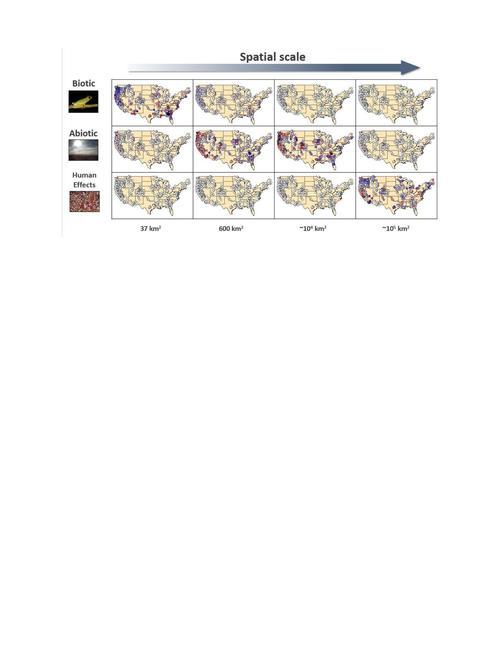
Figure 2.3. Generality of scale-dependent processes in space. Maps indicate the contribution of
each of three processes as predictors of Bd distribution in models. Points represent physical
locations with Bd prevalence data and are colored based on the magnitude of the change in their
residual after the given process was added to a model predicting Bd distribution. Blue, white, and
red points decreased, had no effect, or increased the magnitude of the residuals, respectively.
Maps with many colored points indicate that a given process was highly important at a given
scale, while maps with mostly white points signify that it was unimportant. See Figure A2 for
equivalent maps for WNV and Lyme disease.
Tables
Table 2.1. Results of multi-model inference analyses predicting the prevalence of
Batrachochytrium dendrobatidis. Models used host richness, three abiotic factors, and human
population density as predictors in the analysis. The scales shown are the smallest, intermediate,
and largest scales used. See the Extended Data Table 1 legend for interpretation of the factors and
Table A2 for results for West Nile virus and Borrelia burgdorferi. Statistically significant
(p<.05) predictors are in bold.

Scale/Predictor Estimate Std. Error Pr(>|z|)
1/16th degree
Intercept
0.599
0.025
<0.001
Richness
-0.164
0.028
<0.001
Factor one
-0.011
0.020
0.575
Factor two
-0.021
0.029
0.470
Factor three
0.019
0.025
0.450
Population
0.002
0.010
0.782
1/2 degree
Intercept
0.060
0.026
<0.001
Richness
-0.021
0.049
0.646
Factor one
-0.083
0.031
0.008
Factor two
-0.095
0.033
0.004
Factor three
0.070
0.033
0.035
Population
0.002
0.002
0.993
4 degrees
Intercept
0.587
0.021
<0.001
Richness
-0.002
0.015
0.928
Factor one
-0.005
0.015
0.720
Factor two
-0.006
0.017
0.739
Factor three
0.013
0.028
0.646
Population
-0.177
0.034
<0.001
References
Allan, B. F., R. B. Langerhans, et al. (2009). "Ecological correlates of risk and incidence of West
Nile virus in the United States." Oecologia 158(4): 699-708.
Altizer, S., R. S. Ostfeld, et al. (2013). "Climate Change and Infectious Diseases: From Evidence to
a Predictive Framework." Science 341(6145): 514-519.
Anderson, D. R. (2008). Model based inference in the life sciences : a primer on evidence. New
York ; London, Springer.
Barton, K. (2014). "MuMIn: Multi-Model Inference, R Package version 1.10.0."
Bivand, R. and C. Rundel (2014). "rgeos: Interface to Geometry Engine - Open Source (GEOS),

R package version 0.3-4."
Bjornstad, O. (2015). "ncf: Spatial Nonparametric Covariance Functions."
Burnham, K. P. and D. R. Anderson (2002). Model selection and multimodel inference : a
practical information-theoretic approach. New York, London, Springer.
Chase, J. M. and M. A. Leibold (2002). "Spatial scale dictates the productivity-biodiversity relationship."
Nature 416(6879): 427-430.
Civitello, D. J., J. Cohen, et al. (2015). "Biodiversity inhibits parasites: Broad evidence for the
dilution effect." Proceedings of the National Academy of Sciences of the United States of
America 112(28): 8667-8671.
Dormann, C. F., J. M McPherson, et al. (2007). "Methods to account for spatial autocorrelation in
the analysis of species distributional data: a review." Ecography 30(5): 609-628.
Elith, J., C. H. Graham, et al. (2006). "Novel methods improve prediction of species'
distributions from occurrence data." Ecography 29(2): 129-151.
Glass, G. E., B. S. Schwartz, et al. (1995). "Environmental Risk-Factors for Lyme-Disease
Identified with Geographic Information-Systems." American Journal of Public Health 85(7):
944-948.
Gotelli, N. J., G. R. Graves, et al. (2010). "Macroecological signals of species interactions in the
Danish avifauna." Proceedings of the National Academy of Sciences of the United States of
America 107(11): 5030-5035.
Hijmans, R. J. (2014). "raster: Geographic data analysis and modeling, R package version
2.2.31."
Houghton, J., Y. Ding, et al. (2001). "IPCC 2001: Climate Change 2001." The Climate change
Contribution of Working Group I to the Third Assessment Report of the
Intergovemmental Panel on Climate Change 159.
Johnson , P. T. J., R. S. Ostfeld, et al. (2015). "Frontiers in research on biodiversity and disease."

Ecology Letters in press: in press.
Jones, K. E., N. G. Patel, et al. (2008). "Global trends in emerging infectious diseases." Nature
451(7181): 990-U994.
Keesing, F., L. K. Belden, et al. (2010). "Impacts of biodiversity on the emergence and transmission
of infectious diseases." Nature 468(7324): 647-652.
Kilpatrick, A. M. (2011). "Globalization, land use, and the invasion of West Nile Virus." Science
334(6054): 323-327.
Kilpatrick, A. M., C. J. Briggs, et al. (2010). "The ecology and impact of chytridiomycosis: an emerging
disease of amphibians." Trends in Ecology & Evolution 25(2): 109-118.
Levin, S. A. (1992). "The Problem of Pattern and Scale in Ecology." Ecology 73(6): 1943-1967.
Liu, X., J. R. Rohr, et al. (2013). "Climate, vegetation, introduced hosts and trade shape a global
wildlife pandemic." Proceedings of the Royal Society B-Biological Sciences 280(1753). McGill, B. J.
(2010). "Matters of Scale." Science 328(5978): 575-576.
McKinney, M. L. and J. L. Lockwood (1999). "Biotic homogenization: a few winners replacing
many losers in the next mass extinction." Trends in Ecology & Evolution 14(11): 450453.
Menge, B. A. and J. P. Sutherland (1976). "Species-Diversity Gradients - Synthesis of Roles of
Predation, Competition, and Temporal Heterogeneity." American Naturalist 110(973):
351-369.
Noss, R. F. (1991). Landscape linkages and biodiversity, Island Press: 27-39.
Ostfeld, R. S., G. E. Glass, et al. (2005). "Spatial epidemiology: an emerging (or re-emerging) discipline."
Trends in Ecology & Evolution 20(6): 328-336.
Ostfeld, R. S. and F. Keesing (2000). "Biodiversity and disease risk: The case of lyme disease."
Conservation Biology 14(3): 722-728.
Parmesan, C. (2006). "Ecological and evolutionary responses to recent climate change." Annual
Review of Ecology Evolution and Systematics 37: 637-669.

Pinheiro, J., D. Bates, et al. (2014). "nlme: Linear and Nonlinear Mixed Effects Models, R
package version 3.1-117."
Rahbek, C. (2005). "The role of spatial scale and the perception of large-scale species-richness patterns."
Ecology Letters 8(2): 224-239.
Rohr, J. R., A. P. Dobson, et al. (2011). "Frontiers in climate change-disease research." Trends in
Ecology & Evolution 26(6): 270-277.
Rouget, M. and D. M. Richardson (2003). "Inferring process from pattern in plant invasions: a
semimechanistic model incorporating propagule pressure and environmental factors."
The American Naturalist 162(6): 713-724.
Sandel, B. and A. B. Smith (2009). "Scale as a lurking factor: incorporating scale-dependence in
experimental ecology." Oikos 118(9): 1284-1291.
Tatem, A. J., S. I. Hay, et al. (2006). "Global traffic and disease vector dispersal." Proceedings of the
National Academy of Sciences of the United States of America 103(16): 6242-6247.
Team, R. C. (2014). R: A language and environment for statistical computing. R Foundation for
Statistical Computing, Vienna, Austria.
Trisos, C. H. and O. L. T. Petchey, J. A. (2014). "Unraveling the Interplay of Community Assembly
Processes Acting on Multiple Niche Axes across Spatial Scales." The
American Naturalist 184(5): 593-608.
VectorMapsTeam (2015). "VectorMaps." http://www.vectormap.org/Mosquito_Metadata.htm.
Venesky, M. D., T. R. Raffel, et al. (2014). "Confronting inconsistencies in the
amphibianchytridiomycosis system: implications for disease management." Biological Reviews
89:
477-483.
Wiens, J. A. (1989). "Spatial Scaling in Ecology." Functional Ecology 3(4): 385-397.

Wood, C. L. and K. D. Lafferty (2013). "Biodiversity and disease: a synthesis of ecological
perspectives on Lyme disease transmission." Trends in Ecology & Evolution 28(4): 239247.
CHAPTER THREE:
A GLOBAL SYNTHESIS OF PHENOLOGICAL RESPONSES TO CLIMATE CHANGE
Authors
Jeremy M. Cohen, Marc Lajeunesse5, and Jason R. Rohr5

Abstract
Phenology, or the timing of seasonal activities, is shifting with climate change. However, little is
known about which climatic factors drive phenology across latitudes, the species traits associated
with phenological responses, or why some species have delayed rather than advanced their
phenology in spring. Here, we address these questions by synthesizing 1,011 published time
series of animal phenology. We find that temperature drives phenological responses at
midlatitudes, whereas at lower latitudes precipitation is more important. Body size and
endothermy are negatively associated with the strength of phenological shifts, suggesting
emerging asynchronies between parasites and hosts and predators and prey. Finally, apparent
phenological delays are associated with short annual records prone to sampling error. As climate
change intensifies, our findings arm biologists with information on which climatic variables and
organismal traits drive emerging asynchronies between species.

Main Text
Global climate change has significant ecological consequences (Walther, Post et al. 2002;
Rosenzweig, Karoly et al. 2008) and perhaps the most well-studied are advancements in the
timing of seasonal activities, or phenology, of organisms. This is because phenological shifts can
cause species declines by creating asynchronies or “mismatches” between plants and pollinators
(Hegland, Nielsen et al. 2009), plants and herbivores (Visser and Holleman 2001; Visser and Both
2005; van Asch, Tienderen et al. 2007), migrant birds and their prey (Moller, Rubolini et al.
2008; Both, Van Turnhout et al. 2010), and hosts and parasites (Mas-Coma, Valero et al. 2009).
Although advancements in the phenology of plants and animals have been widely reported and
synthesized (Parmesan and Yohe 2003; Root, Price et al. 2003; Gienapp, Leimu et al. 2007;
Thackeray, Henrys et al. 2016), there remain several open knowledge gaps. First, although many
phenological studies and syntheses assume climate change as an important driver, few explicitly
test for any effect of climate, but among those that do, standardized climate data are often not
used to confirm the link between changes in phenology and climate. As a consequence, it
remains unclear which climatic variables are driving shifts in phenology and whether
geographical heterogeneity in these variables has impacted their predictive power to detect
ecological trends. Second, there is controversy regarding why some species have apparently
delayed spring phenologies despite an overall predicted trend towards advancement (Barbraud
and Weimerskirch 2006; Yu, Luedeling et al. 2010). Finally, it is unclear which species-level
traits (e.g., body size, thermy) are associated with strong phenological shifts, although a recent
analysis found associations between trophic level and phenological responses in the UK
(Thackeray, Henrys et al. 2016). Because of these gaps in the literature, a general global framework in the
climate sciences is still missing for predicting the direction and magnitude of phenological shifts based
on ecological context and organismal traits.

To address these gaps, we conducted a global synthesis of 1,011 phenological time series of
animals from 127 studies (Table B1; Table B2), spanning five continents and 15 classes of
animals including insects, mammals, reptiles, and birds. We focused on animals because the
evidence for advancement in phenology is more conflicting and controversial than it is for plants
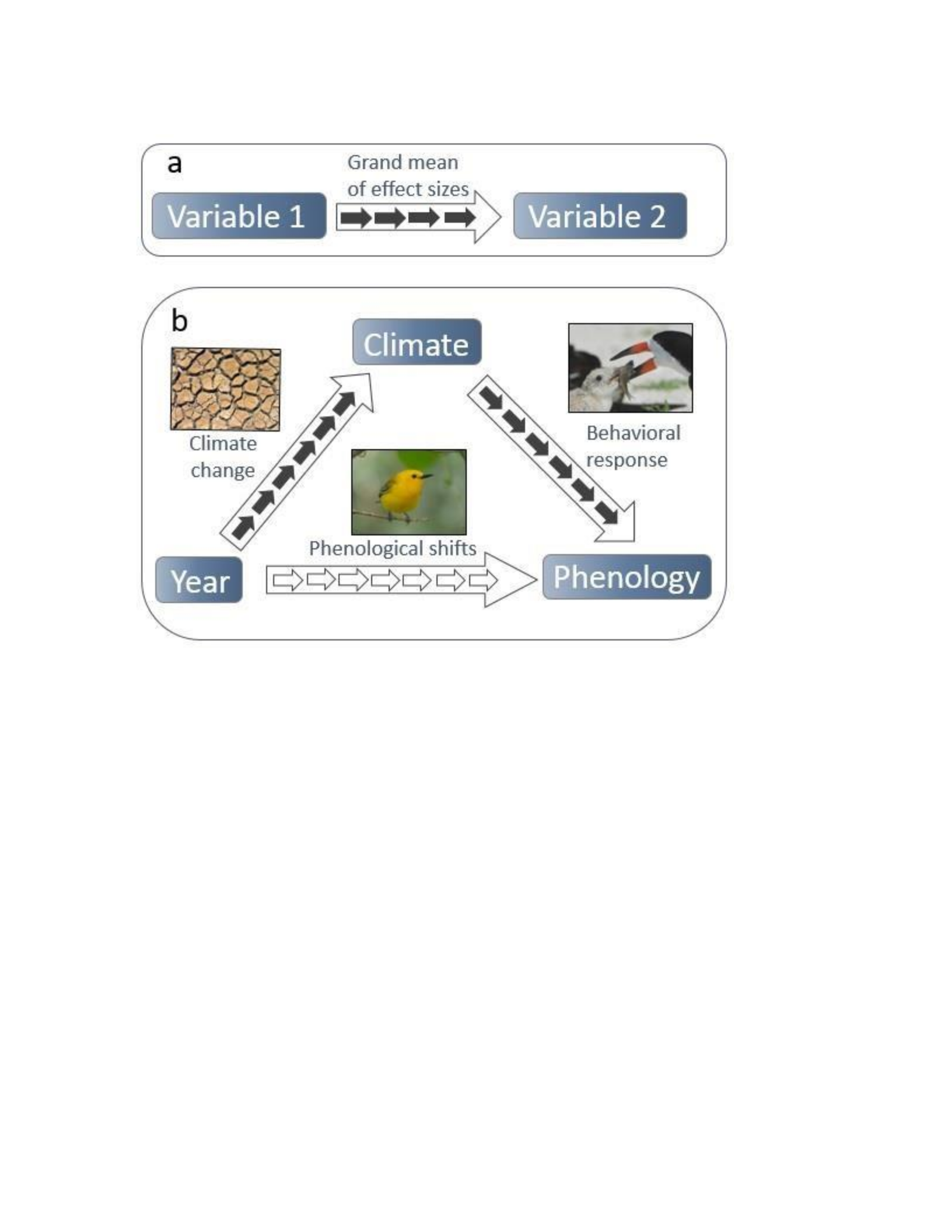
(Menzel, Sparks et al. 2006). We utilized a unique mixed-model trivariate meta-analysis to
synthesize the pairwise correlations between phenology, climate, and sampling year (Fig. 3.1; see
Methods) and to explore species, climate, and geographic predictors of phenology. Unlike
previous syntheses, our meta-analysis uses hierarchical random-effects modeling to account for
1) experimental covariances within and among dependent outcomes of phenological correlations
(Lajeunesse 2011) and 2) the lack of independence because of the shared phylogenetic histories
of taxa ((Lajeunesse 2009); see Supplementary Code). Moreover, our climate variables (including
mean, minimum and maximum temperature, precipitation, snowfall (Inouye, Barr et al. 2000),
and others, see Methods) were standardized across all time series by accessing a single source of
historical climate data (NOAA’s NCDC-3 dataset (Lawrimore, Menne et al. 2011)) with data that
was specific to the region and time of each study, allowing us to reliably identify which aspects
of climate were driving phenological shifts. Importantly, this approach facilitated our evaluation
of whether climate change (the 50 year correlation between climate and year), rather than just
climate, was associated with changes in phenology. Further, our approach also tests whether the
annual peaks and valleys in climate and phenology generally match up, which has many fewer
causal explanations than a correlation between climate and phenology across multiple decades
(Rohr and Raffel 2010).
The meta-analysis revealed that, on average, animals have advanced their phenology
significantly since 1950 ( =-0.318, df=937, p=0.01; Fig. 3.2a; Table B3). Across all species and
sites, mean temperature increased significantly over time (Fig. 3.2a; Table S4). The metaanalysis
also revealed that the larger the increase in temperature through time at a location, the earlier the

phenology, suggesting that climate change is indeed the causal driver of these shifts (Fig. 3.2a;
Table B4). Phenological shifts were not heavily biased by the phylogenetic history of taxa, which
accounted for only about 4.5% of the variance between phenology and year, and 06% between
phenology and climate (Tables B3-8). Within-study variance accounted for 8-9% of the total
variance accounted for in all models (Tables B3-8).
There has been debate over why some species appear to have delayed, rather than advanced,
their phenology (Barbraud and Weimerskirch 2006; Lane, Kruuk et al. 2012). We hypothesized
that these apparent delays were generally spurious artifacts of studies with few annual records. A
funnel plot revealed that many studies based on short time series (e.g., small sample sizes) had both
delays and strong advances in phenology, but when sample sizes were large, phenology advanced
more uniformly (Fig. 3.2b). While this result does not rule out the possibility of true delays in
phenology in some instances, it suggests that many of the reported delays in phenology are likely
specious and sensitive to sampling error. Previous phenological syntheses did not properly down-
weight these studies with low sample sizes and high variances and thus underestimated
phenological advancements.
We also hypothesized that phenological shifts would be associated with climatic variables that
drive seasonality locally. Hence, we predicted that phenological shifts would be associated with
temperature at mid-latitudes (i.e. temperate zones) and precipitation at low latitudes (i.e. tropical
and subtropical zones). Moreover, because climate change is causing greater changes in
temperature than precipitation (Field and Van Aalst 2014), we expected to see greater
phenological shifts in temperate than tropical zones. In support of these hypotheses, as absolute
value of latitude increased, changes to temperature became more predictive of the magnitude of
phenological shifts, but as latitude decreased, precipitation became a stronger predictor of
phenology (test for different slopes: t=7.89, df=1650, p<0.0001; Fig. 3.2c; Table B5).
Additionally, temperature changed more through time than did precipitation (Fig. B1), and the

association between phenology and temperature in the temperate zones was stronger than the
association between phenology and precipitation in the tropics (Fig. 3.2c). These results indicate
that different climatic variables are triggering phenology in temperate and tropical regions. While
past syntheses have hypothesized that species should shift their phenology faster at higher
latitudes in response to greater warming in these regions (Parmesan and Yohe 2003; Root, Price et
al. 2003; While and Uller 2014), low-latitude species may also be shifting their phenology at high
rates in response to changes in rainfall. Given that the majority of phenological studies have
occurred in northern temperate climates (especially North America and Europe; Fig. 3.3), and
emphasized temperature over precipitation, additional phenological time series from low latitudes
are needed to more accurately quantify the effects of changes to precipitation on tropical
phenology.
Because so many phenological studies have been conducted in temperate regions where
temperature drives seasonality and phenology, we hypothesized that the phenology of specific
taxonomic groups would be more strongly associated with temperature than precipitation. For
example, we expected amphibians to respond to precipitation more strongly than any other taxon
because of their considerable reliance on moist conditions for survival and reproduction.
However, across all taxa, phenology was associated more strongly with temperature than with
precipitation (temperature, =-0.310, df=1579, p=0.02; precipitation, =-0.054, df=1579, p=0.54; Fig.
B2; Table B4), and different components of temperature (mean, minimum and maximum) did not
significantly differ from one another at predicting phenology. Among all taxa, amphibians exhibited the
strongest association between precipitation and phenology ( =-
0.172, p=0.16; Fig. B2b; Table B6).
Next, we sought to identify general characteristics of species that might be predictive of the
strength of their phenological responses to climate. We hypothesized that thermy and body size
would generally predict the strength of phenological shifts because ectotherms and smaller

organisms should be more sensitive to shifts in climate than endotherms and larger organisms
(because thermal inertia is positively associated with body size; (Gillooly, Brown et al. 2001;
Rohr, Civitello et al. in review)). As predicted, the phenology of ectotherms was more strongly
correlated with temperature than the phenology of endotherms (Fig. 3.4a; Table B7), and body
size was a significant negative predictor of phenological shifts alone (β=-0.0221, df=921,
p<0.01; Table B7) and as a covariate alongside other organismal traits in most statistical models
(Fig. 2d; Table B7). Among taxa, invertebrate groups, such as butterflies, closely tracked their
phenology to temperature while birds and mammals did not (Fig. 4b; Table B7), and as a whole,
invertebrates tended to track temperature better than vertebrates (Fig. 4c; Table B7). Herbivore
phenology tracked temperature more closely than carnivore phenology (Fig. 4d; Table B7) when
accounting for body size, possibly because herbivores are also responding to shifts in the timing
of plant phenology (Ovaskainen, Skorokhodova et al. 2013), as demonstrated in a recent UKwide
synthesis of phenological responses to climate change (Thackeray, Henrys et al. 2016).
Additionally, we did not observe a difference between the phenological responses of terrestrial and
aquatic species (Fig. B3; Table B7), although there are admittedly few aquatic species in the dataset (18
total) and all are marine.
Finally, we posited that certain phenological endpoints might be more sensitive to climate
change than others. We grouped phenological endpoints into three categories, abundance (peak
seasonal abundance), arrival (migration), and breeding/rearing (calling, nesting, laying, hatching,
or weaning), and predicted that arrival would be least correlated with climatic factors because
migrants are likely reacting to climatic conditions where they left from rather than conditions to
where they are arriving (Lehikoinen, Sparks et al. 2004). Phenological endpoints based on
arrival tracked climate most poorly (Fig. B4; Table B8), and those based on abundance tracked
temperature changes the most closely; possibly because abundance is more often documented
with smaller invertebrates that phenologically respond strongly to climate. Because there is a

paucity of phenological time series from equatorial regions, and arriving species often come
from multiple departure locations, we unfortunately could not test whether the timing of
departures for spring migrations tracked temperature better than arrivals (but see (Gordo 2007)).
Our findings add to the growing evidence of direct ecological consequences of climate
change on ecological systems. By accounting for the lack of independence among effect sizes,
taxa, and studies, standardizing and detrending our climate and phenology data, and conducting a
weighted mixed-effect meta-analysis across all animal taxa, we provide the strongest causal
evidence to date linking climate change to phenological shifts. Additionally, our analyses
unveiled previously unidentified generality in the phenological responses of organisms to
climate. Our synthesis indicates that animals are generally advancing their phenologies and that
reported delays in phenology are likely a product of sampling error because of too few sampling
years to fully assess long-term trends. Further, we show that the phenology of species at high
and low latitudes most strongly respond to temperature and precipitation, respectively, and thus
different components of climate drive phenology in different regions of the globe. However, the
scarcity of phenological time series from low latitudes and marine systems makes it challenging
to obtain precise estimates of the relationship between climate change and phenology in these
regions; we encourage climate biologists to fill these gaps. We also show that different taxa
respond to the same climatic signals but do so at different rates. Importantly, the strength of
these phenological shifts is predictable based on two easily measured traits of species, their
thermy and body size, with the phenology of smaller organisms and ectotherms responding more
strongly to climate change than larger organisms and endotherms. As climate change intensifies
in the next century, our results suggest that advances in phenology are likely to become more
exaggerated, potentially further desynchronizing interactions between species that vary
considerably in their body sizes, such as mutualistic, predator-prey, and host-parasite
interactions. However, the synthesis presented here now arms climate biologists with knowledge

on the specific components of climate and the traits of interacting species (differences in the
body sizes and thermy) that can drive asynchronies, providing new opportunities to forecast
mismatches and mitigate their adverse effects.
Acknowledgements
We thank N. Argento and C. Gionet for assistance extracting data from studies, T. James for
assistance compiling references, and D. Civitello, B. Delius, N. Halstead, S. Knutie, K. Nguyen,
N. Ortega, B. Roznik, E. Sauer and S. Young for comments on the manuscript. This research was
supported by grants from the National Science Foundation to M.J.L (DBI-1262545, DEB1451031)
and J.R.R. (EF-1241889, DEB-1518681), and National Institutes of Health (R01GM109499,
R01TW010286), US Department of Agriculture (NRI 2006-01370, 2009-
35102-0543), and US Environmental Protection Agency (CAREER 83518801) to J.R.R.
Figures
Figure 3.1. Structure of trivariate meta-analysis examining the relationship between
phenology, climate, and year. Conceptual schema contrasting the structure of (a) a typical meta-
analysis summarizing the relationship (correlation) between two variables using the grand mean
of one effect size (large arrows) composed of many effect sizes reported in the literature (small
arrows) and (b) the trivariate meta-analysis used in this study which summarizes the relationship
among three variables using three effect sizes (standardized correlations). Filled arrows represent
direct effects (i.e., the effect of climate on phenology) and open arrows represent indirect effects
(i.e., the effect of year on phenology). This trivariate meta-analysis allowed us to jointly analyze
the three effect sizes quantifying the pairwise relationships between phenology, time, and
climate. Further, it enabled us to account for the correlations within the three non-independent
effect sizes (because of common sampling variability), while also explicitly accounting for any
existing correlations among them (via a multivariate randomeffects model). See Methods and
Appendix A for further details.
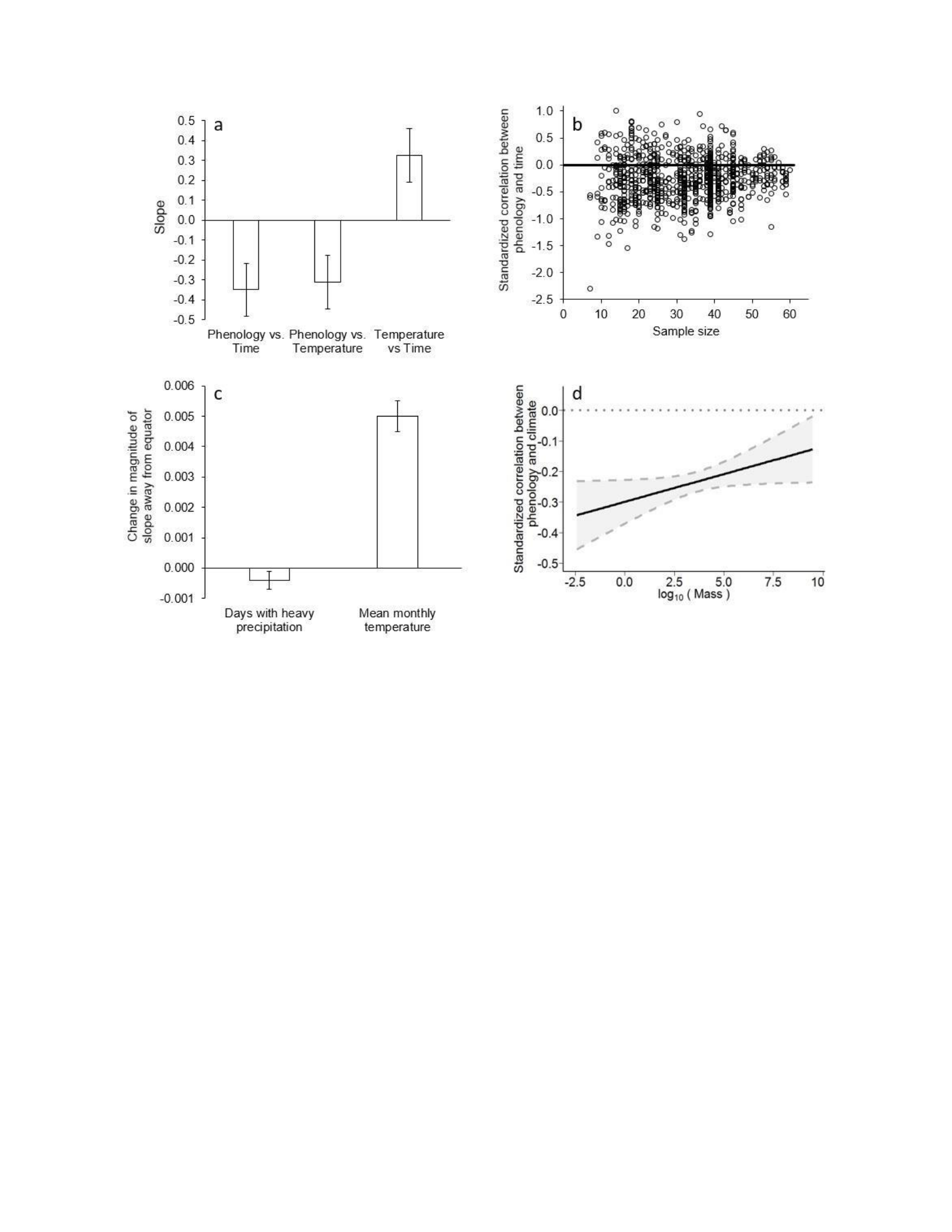
Figure 3.2. Improving how we understand of advancements in phenology. (a) Across 1,011
time series, phenology became earlier through time as temperature increased through time and
the detrended increases in temperature were negatively correlated with phenology. Error bars
represent standard errors. (b) A funnel plot comparing sample sizes (total years in time series
length) with standardized effect sizes (correlation between phenology and time; Z effect sizes)
reveals that studies with small samples sizes have large variation with both the positive and
negative shifts suggesting that species appearing to delay their phenology might be spurious
products of sampling error. (c) Temperature became more predictive of phenology as the absolute
value of latitude increased (bars represents slope between latitude and the relationship between
climate and phenology, p<0.0001), whereas rainfall became predictive of phenology as the
absolute value of latitude decreased (p<0.01, test for different slopes: p<0.0001), suggesting that
the phenology of species is driven by the climatic factor that locally drives seasonality. Error bars
represent standard errors. (d) The slope between log-transformed body mass and the correlation
between phenological date and mean temperature is positive in the trivariate metaanalysis model,
indicating that smaller organisms track their phenology with temperature more closely than larger
organisms. Data points are not shown to reduce clutter, but 95% confidence bands are provided
in gray.

Figure 3.3. Distribution of published studies exploring the phenology of animals. There are
hundreds of published phenology time series from North America and Europe, but much less is
known about phenology on the other five continents with particularly large gaps in tropical
regions and marine systems. Red points indicate advancements in phenology over time and blue
points indicate delays. The strength of the color indicates the magnitude of the relationship
between phenology and time.
Figure 3.4. The ability of phenology to track temperature varies with taxonomy, thermy,
and trophic level. After controlling for body size, (a) smaller taxa, such as (b) invertebrates, and
(c) ectotherms tracked temperature closer than larger animals and endotherms. (d) Herbivores
had a greater association between temperature and phenology than carnivores (controlling for

body size), possibly because herbivores were reacting to shifts in plant phenology associated
with temperature. Error bars represent standard errors for the slope parameters from
mixedmodel meta-regressions. Different letters denote statistically significant differences in
effect size.
References
Barbraud, C. and H. Weimerskirch (2006). "Antarctic avian phenology and climate change."
Journal of Ornithology 147(5): 52-52.
Barbraud, C. and H. Weimerskirch (2006). "Antarctic birds breed later in response to climate
change." Proceedings of the National Academy of Sciences of the United States of America
103(16): 6248-6251.
Both, C., C. A. M. Van Turnhout, et al. (2010). "Avian population consequences of climate change
are most severe for long-distance migrants in seasonal habitats." Proceedings of the Royal
Society B-Biological Sciences 277(1685): 1259-1266.
Field, C. B. and M. Van Aalst (2014). Climate change 2014: impacts, adaptation, and
vulnerability, IPCC.
Gienapp, P., R. Leimu, et al. (2007). "Responses to climate change in avian migration time -
microevolution versus phenotypic plasticity." Climate Research 35(1-2): 25-35.
Gillooly, J. F., J. H. Brown, et al. (2001). "Effects of size and temperature on metabolic rate."
Science 293(5538): 2248-2251.
Gordo, O. (2007). "Why are bird migration dates shifting? A review of weather and climate effects
on avian migratory phenology." Climate Research 35(1-2): 37-58.
Hegland, S. J., A. Nielsen, et al. (2009). "How does climate warming affect plant-pollinator interactions?"
Ecology Letters 12(2): 184-195.
Inouye, D. W., B. Barr, et al. (2000). "Climate change is affecting altitudinal migrants and hibernating
species." Proceedings of the National Academy of Sciences of the United
States of America 97(4): 1630-1633.

Lajeunesse, M. J. (2009). "Meta-Analysis and the Comparative Phylogenetic Method." American
Naturalist 174(3): 369-381.
Lajeunesse, M. J. (2011). "On the meta-analysis of response ratios for studies with correlated and multi-
group designs." Ecology 92(11): 2049-2055.
Lane, J. E., L. E. B. Kruuk, et al. (2012). "Delayed phenology and reduced fitness associated
with climate change in a wild hibernator." Nature 489(7417): 554-+.
Lawrimore, J. H., M. J. Menne, et al. (2011). "An overview of the Global Historical Climatology
Network monthly mean temperature data set, version 3." Journal of Geophysical Research-
Atmospheres 116.
Lehikoinen, E., T. H. Sparks, et al. (2004). "Arrival and departure dates." Birds and Climate
Change 35: 1-31.
Mas-Coma, S., M. A. Valero, et al. (2009). "Climate change effects on trematodiases, with emphasis
on zoonotic fascioliasis and schistosomiasis." Veterinary Parasitology 163(4):
264-280.
Menzel, A., T. H. Sparks, et al. (2006). "European phenological response to climate change matches
the warming pattern." Global Change Biology 12(10): 1969-1976.
Moller, A. P., D. Rubolini, et al. (2008). "Populations of migratory bird species that did not show a
phenological response to climate change are declining." Proceedings of the National
Academy of Sciences of the United States of America 105(42): 16195-16200.
Ovaskainen, O., S. Skorokhodova, et al. (2013). "Community-level phenological response to
climate change." Proceedings of the National Academy of Sciences of the United States of
America 110(33): 13434-13439.
Parmesan, C. and G. Yohe (2003). "A globally coherent fingerprint of climate change impacts across
natural systems." Nature 421(6918): 37-42.

Rohr, J., D. J. Civitello, et al. (in review). "A global framework for estimating acclimation and
thermal breadth predicts risk from climate change " Proceedings of the National Academy
of Sciences of the United States of America.
Rohr, J. R. and T. R. Raffel (2010). "Linking global climate and temperature variability to widespread
amphibian declines putatively caused by disease." Proceedings of the
National Academy of Sciences of the United States of America 107(18): 8269-8274.
Root, T. L., J. T. Price, et al. (2003). "Fingerprints of global warming on wild animals and plants."
Nature 421(6918): 57-60.
Rosenzweig, C., D. Karoly, et al. (2008). "Attributing physical and biological impacts to anthropogenic
climate change." Nature 453(7193): 353-U320.
Thackeray, S. J., P. A. Henrys, et al. (2016). "Phenological sensitivity to climate across taxa and trophic
levels." Nature.
van Asch, M., P. H. Tienderen, et al. (2007). "Predicting adaptation of phenology in response to climate
change, an insect herbivore example." Global Change Biology 13(8): 1596-1604.
Visser, M. E. and C. Both (2005). "Shifts in phenology due to global climate change: the need for
a yardstick." Proceedings of the Royal Society B-Biological Sciences 272(1581):
2561-2569.
Visser, M. E. and L. J. M. Holleman (2001). "Warmer springs disrupt the synchrony of oak and winter
moth phenology." Proceedings of the Royal Society B-Biological Sciences
268(1464): 289-294.
Walther, G. R., E. Post, et al. (2002). "Ecological responses to recent climate change." Nature
416(6879): 389-395.
While, G. M. and T. Uller (2014). "Quo vadis amphibia? Global warming and breeding phenology
in frogs, toads and salamanders." Ecography 37(10): 921-929.

Yu, H. Y., E. Luedeling, et al. (2010). "Winter and spring warming result in delayed spring
phenology on the Tibetan Plateau." Proceedings of the National Academy of Sciences of the
United States of America 107(51): 22151-22156.
1

51
CHAPTER FOUR:
THE THERMAL MISMATCH HYPOTHESIS EXPLAINS OUTBREAKS OF AN
EMERGING INFECTIOUS DISEASE
Authors
Jeremy M. Cohen, Matthew D. Venesky, Erin L. Sauer7, David J. Civitello7, Taegan A.
McMahon, Elizabeth A. Roznik7, Jason R. Rohr7

52
Abstract
Parasites typically have broader performance breadths than hosts, and thus large performance
gaps between pathogens and their cold- and warm-adapted hosts should occur at relatively warm
and cold temperatures, respectively. We tested this thermal mismatch hypothesis by quantifying
the temperature-dependent susceptibility of cold- and warm-adapted amphibian species to the
fungal pathogen Batrachochytrium dendrobatidis (Bd) using laboratory experiments and field
prevalence estimates from 4,775 host populations. In both the laboratory and field, we found that
peak susceptibility for cold- and warm-adapted hosts occurred at relatively warm and cool
temperatures, respectively, providing support for the thermal mismatch hypothesis. Our results
suggest that as climate change shifts hosts away from their optimal temperatures, the probability
of infectious disease outbreaks might increase, but the effect will depend on the host species and
the direction of the climate shift. Our findings help explain the tremendous variation in species
responses to Bd and climate change and spatial, temporal, and species-level variation in outbreaks
associated with extreme weather events that are becoming more common with climate change.
Introduction
One of the most important ecological crises affecting humans and biodiversity is the
recent increase in emerging infectious diseases (Daszak 2000; Anderson, Cunningham et al. 2004;
Jones, Patel et al. 2008). Since 1950, hundreds of emerging infectious diseases have been
recorded (Jones, Patel et al. 2008), causing widespread declines of individual species and
biodiversity in general (Daszak 2000; Skerratt, Berger et al. 2007; Fisher, Henk et al. 2012).
Many infectious disease outbreaks are associated with extreme weather events, including
outbreaks of malaria, dengue, cholera, and amphibian and coral diseases (Cazelles, Chavez et al.
2005; Koelle, Rodo et al. 2005; Bruno, Selig et al. 2007; Pascual, Cazelles et al. 2008; Rohr and

53
Raffel 2010). To combat these outbreaks, it is critical that researchers understand the precise
environmental conditions that promote them, especially with rapidly changing climates and other
sources of human-induced stress on wildlife populations (Rohr, Dobson et al. 2011).
Although it is clear that extreme weather events cause disease outbreaks, it is also clear
that neither warm nor cold spells universally increase outbreaks (Rohr, Dobson et al. 2011). Thus,
more nuanced hypotheses regarding the effects of weather and climate on disease are necessary.
For example, Nowakowski et al. (2016) recently argued that the degree of mismatch between
critical thermal tolerances of hosts and parasites might drive disease outbreaks. Similarly, thermal
mismatches in temperature optima can occur within host-parasite interactions when cold-adapted
hosts and parasites experience warm spells and vice versa. This latter notion addresses the
difference between current or recent temperatures and the long-term mean temperature to which
the local hosts and parasites have evolved; thus, it highlights the role of environmental variability,
particularly extreme weather events. If these mismatches are predictive of parasite transmission,
they could explain spatial, temporal, and species-level variation in outbreaks associated with
extreme weather events that are becoming more common with climate change (Rosenzweig,
Iglesias et al. 2001; Anyamba, Small et al. 2014).
Here, we propose and test the thermal mismatch hypothesis, which posits that hosts should
be more susceptible to outbreaks when environmental conditions shift away from their optima
(Fig. 4.1). This hypothesis is based on a few assumptions. First, we assume that hosts and
parasites are locally adapted to their thermal environments (Laine 2008; Sternberg and Thomas
2014). Although we show in Fig. 4.1 the temperature optima of the host and parasite to be
identical because of local adaptation (Fig. 4.1a,b), we acknowledge that they can be different for
several reasons (e.g. different microclimates or breeding times). Even if they are different, the key
underlying assumption is that hosts and parasites adapted to similar climates will have more

54
similar temperature optima than hosts and parasites adapted to different climates. As long as this
assumption holds, the predictions of the heuristic framework remain the same. Second, we
assume that the performance of cold- and warm-adapted hosts and parasites in isolation are
approaching their lower and upper thermal limits, respectively, and thus have right- and
leftskewed thermal performance curves, respectively (Fig. 4.1a,b). Third, small organisms, such
as pathogens, generally have broader thermal breadths than larger organisms, such as hosts
(BaasBecking 1934). Indeed, a recent meta-analysis of thermal performance curves revealed that
body mass was a significant negative predictor of thermal breadths (Rohr, Civitello et al. in
review).
Hence, we assume that parasites have broader thermal breadths than hosts (Fig. 4.1a,b).
Temperatures where the thermal performance of the parasite most exceeds that of the host
(arrows in Fig. 4.1a,b and peak in Fig. 1c,d) might be where outbreaks are most likely, and thus,
subtracting the thermal performance curves of the hosts and parasites in isolation (Fig.
4.1a,b) offers a hypothesis for their thermal performance when interacting (Fig. 4.1c,d). The
outcome of this subtraction produces two predictions, one about the temperature of maximal
parasite growth on hosts and the other about the shape of the thermal performance curve of
parasite growth on hosts. First, as a consequence of the broader breadths of parasites and the
physiological upper and lower limits of temperature tolerances of both hosts and parasites (i.e. the
right- and left-skewed curves for isolated cold- and warm-adapted organisms, respectively; Fig.
4.1a,b), hosts should, on average, be susceptible to outbreaks when temperatures most greatly
differ from the temperature to which they are evolved (i.e. long-term average temperature;
(Raffel, Rohr et al. 2006; Fitt, Gates et al. 2009). Or, in other words, parasite prevalence and
abundance for cold-and warm-adapted hosts should be maximized at warm and cool
temperatures, respectively (Fig. 4.1). We emphasize that this prediction is robust to the above

55
underlying assumptions regarding local adaptation of hosts and parasites and skew of thermal
performance curves (Fig. C1). The second prediction is that, despite cold- and warm-adapted
hosts and parasites having right- and left-skewed thermal performance curves in isolation (Fig.
4.1a,b), the thermal performance curves of parasite growth on cold- and warm-adapted hosts (i.e.,
when interacting) should be left- and right-skewed, respectively (Fig. 4.1c,d). If this thermal
mismatch hypothesis is supported, cold-adapted hosts should face considerable risk of parasite
transmission in particularly warm periods and thus they should be most at risk from global
warming-driven disease outbreaks.
We set out to test the thermal mismatch hypothesis using the amphibian-
Batrachochytrium dendrobatidis (Bd, or chytrid fungus) host-parasite system. Outbreaks of this
emerging fungal pathogen are associated with hundreds of amphibian extinctions in the last 50
years (Skerratt, Berger et al. 2007; Rohr and Raffel 2010) and have occurred under a wide variety
of conditions in different hosts (Retallick, McCallum et al. 2004; Bosch, Carrascal et al. 2007;
Whitfield, Kerby et al. 2012). Thus, Bd outbreaks may be predictable based on the thermal
mismatch hypothesis. Bd outbreaks are thought to be directly controlled by climatic conditions
because Bd has a free-living stage and grows on the external skin of its ectothermic hosts
(Kilpatrick, Briggs et al. 2010; Venesky, Raffel et al. 2014) and environmental temperature has
been predictive of Bd outbreaks in a number of large-scale analyses (Murray, Retallick et al.
2011; Liu, Rohr et al. 2013; Cohen, Civitello et al. 2016). Bd grows best under cool conditions in
lab culture (18-22 °C) and is generally not as prevalent under warmer field conditions (Retallick,
McCallum et al. 2004; Kilpatrick, Briggs et al. 2010), and therefore, it has been assumed that cool
conditions typically precede outbreaks. However, retrospective correlations between climate data
and previous Bd outbreaks have led researchers to conflictingly conclude that cool (Retallick,
McCallum et al. 2004; Kriger and Hero 2007; Whitfield, Kerby et al. 2012), dry (Lampo,

56
Rodriguez-Contreras et al. 2006; Laurance 2008), warm (Ron, Duellman et al. 2003; Bosch,
Carrascal et al. 2007), and wet (Kriger and Hero 2007; Puschendorf, Carnaval et al. 2009)
conditions are predictive of high Bd prevalence (Venesky, Raffel et al. 2014). The explanation for
these seemingly contradictory patterns may be that host species or Bd isolates exhibit different
performances across a range of climatic conditions. In fact, this is what would be expected given
the immense variation in climatic conditions that hosts and isolates have been exposed to
throughout time for this global epizootic (Thomas and Blanford 2003; Rohr, Dobson et al. 2011).
To test the thermal mismatch hypothesis experimentally, we quantified 1) host temperature
preferences (proxy of host performance in isolation), 2) temperature-dependent growth rates of
Bd isolates in culture (parasite performance in isolation), and 3) temperaturedependent growth
rates of Bd isolates grown on their local hosts (host and parasite performance when interacting).
These experiments were conducted on three phylogenetically, phenotypically, and ecologically
diverse hosts: Cuban tree frogs (Osteopilus septentrionalis), Southern toads (Anaxyrus terrestris),
and Panamanian golden frogs (Atelopus zeteki). Osteopilus septentrionalis and An. terrestris are
adapted to warm lowland subtropical habitats, whereas At. zeteki are native to cool, high-
elevation cloud forests in Central America. Thus, we predicted that the optimal temperature for
Bd growth on relatively warm-adapted O. septentrionalis and An. terrestris would be lower than
for the relatively cold-adapted At. zeteki. Finally, to assess the generality of our hypothesis, we
searched the literature and collected 4,775 records of amphibian populations (1,270 species)
previously tested for Bd in the field, along with climate data specific to the dates and locations of
testing. We predicted that across all of these populations and species, amphibians in warmer
climates would have peak Bd prevalence at cooler temperatures than species in cooler climates.

57
Materials and Methods
Animal Collection and Maintenance
Adult O. septentrionalis and An. terrestris were collected from Hillsborough County,
Florida, and adult At. zeteki were obtained from the Maryland Zoo (Baltimore, MD)
approximately one month before each species was exposed to Bd across a temperature gradient.
Bd has never been detected on frogs collected from the Tampa, Florida region; thus, these frogs
are unlikely to have a history of Bd exposure. All animals were maintained individually in vented
plastic containers (26 x 16 x 8cm) on top of two folded paper towels soaked with 15mL of
artificial spring water. Animals were fed vitamin and mineral-dusted crickets ad libitum and
containers and paper towels were changed twice weekly. Prior to the experiment, animals were
maintained in a lab at 21°C on a 12h photoperiod for approximately 2 months before being
moved to incubators.
Host Temperature Preference Experiment
To ascertain the preferred temperatures of An. terrestris, O. septentrionalis, and At. zeteki,
we maintained uninfected animals individually in thermal gradient apparatuses (Sauer, Sperry et
al. 2016; n = 24, 25, and 9 animals, respectively). Apparatuses were built out of insulated
aluminum downspout gutters cut into dimensions of 137 x 8 x 6 cm and had ice packs (changed
every 12h and frozen at -80°C) under one end and heat tape under the other. Each apparatus was
sealed on top using five 27 x 10 cm Plexiglas® sheets resting on window weather-stripping.
Organic sphagnum moss served as a substrate within the apparatuses and kept humidity between
84.1-90.7% across the temperature gradient. The apparatuses maintained a consistent temperature
gradient across and within gutters (mean ± SD; cold end 9.29 ± 1.33°C, warm end 33.94 ±

58
0.46°C) and the room was kept on a 12h light cycle. See Sauer et al. (2016) for additional details
about the apparatuses. Animals were maintained in the apparatuses for four days and we took
temperature readings of each frog and the substrate occupied by each frog four times a day
(10:00, 14:00, 18:00, and 22:00) using an Extech® High Temperature Infrared Thermometer
(accuracy: ±2% of rdg < 932°F, emissivity 0.95), which non-invasively measures temperatures
accurately (Rowley and Alford 2007). We averaged each individual’s mean preferred temperature
throughout the trials to determine the overall temperature preference for each species. We
excluded data from individuals whose preferences were more than three standard deviations from
the mean, which were considered to be extreme outliers (we only removed one At. zeteki and one
O. septentrionalis).
Bd Growth Experiments
Hosts and Bd cultures were contained in individual Styrofoam incubators (inner
dimensions 37 x 21 x 13 cm; Marko Foam Products, Salt Lake City, UT; Fig. C2) that had a
double-pane Plexiglas window in the lid to allow light in and were set to 14, 18, 22, 26, or 28°C
(± 0.5°C; for more details, see Raffel, Romansic et al. 2013). Incubators were stored in a GR48
environmental chamber (Environmental Growth Chambers, Chagrin Falls, OH) that maintained
14°C and a 12hr photoperiod. We also exposed An. terrestris to 10°C in identical incubators
inside of a separate chamber (Hotpack® model #352632, Philadelphia, PA). We attempted to
acclimate O. septentrionalis to 10°C but the frogs died during acclimation, and we could not
obtain permission from the Maryland Zoo to expose At. zeteki to 10°C. Incubator temperatures
were monitored throughout the experiments using 15 rotated Hobo pendant temperature/light data
loggers (Onset Computer Corporation, Pocasset, MA).

59
We matched the Bd isolates used in each experiment to the approximate geographic
locations where the frogs were collected. Therefore, we exposed At. zeteki to Bd isolate JEL 423,
which was isolated from a Hylomantis lemur during an epidemic at El Copé, Panamá in 2004.
Osteopilus septentrionalis and An. terrestris were exposed to Bd isolate SRS 812, originally
isolated from a Lithobates catesbeianus captured in the southeastern USA in 2006. Bd cultures
(grown in 1% tryptone broth) were maintained at 21°C for one month before use in the
experiments. We also compared growth curves of these isolates to temperature-dependent growth
curves previously reported in the literature, specifically isolate 197 from Washington, D.C.
(Piotrowski, Annis et al. 2004) and isolate 98-1469/10 from Victoria, Australia (Woodhams,
Alford et al. 2008), to examine whether there was variation in optimal temperatures for growth in
culture across these isolates. We also wanted to determine whether variation between isolates was
responsible for any variation in temperature-dependent growth of Bd on hosts.
All hosts were acclimated to their exposure temperature within incubators for 14 days
prior to Bd exposure (n = 6 for An. terrestris and O. septentrionalis; n = 8 for At. zeteki per
temperature). Thus, we avoided two issues common to temperature/disease experiments:
pseudoreplication within temperature treatments and the confounding of exposure to a parasite
with acclimation to a new temperature (Rohr, Dobson et al. 2011). We acclimated Bd to each
temperature for 12 hr before exposing the frogs. To standardize these cultures, zoospores were
counted from 10 µl aliquots of broth using a hemocytometer and Trypan blue (McMahon and
Rohr 2014) and were diluted with sterile 1% tryptone to a common concentration (see below).
We conducted two separate experiments in which we exposed frogs to Bd over a
temperature gradient: the US Species Experiment (with An. terrestris and O. septentrionalis as
hosts) and the Atelopus Experiment (with At. zeteki as a host), the latter of which was conducted
over two temporal blocks (see below). In the US Species Experiment and block 1 of the Atelopus

60
Experiment, all animals were exposed to Bd (see below) because our focus was on Bd growth
rates across temperatures and we expected low mortality over the four-week experiment, as
Bdinduced amphibian mortality is generally low for at least a month post-exposure. However, we
had unexpectedly high mortality of At. zeteki and thus, in the second temporal block of the
Atelopus Experiment (conducted with new animals), we added control individuals (exposed to 1%
tryptone broth not containing Bd) at all temperature treatments. After acclimation, the animals
were weighed and exposed to 3.75x10⁵ zoospores of the appropriate Bd isolate in 3mL tryptone
broth. Bd was pipetted directly on the back of each animal and runoff remained in the container
with the animal for 24hrs before a paper towel change. Bd growth on frogs was measured by
swabbing the right hind limb of each frog one, two and four weeks after Bd exposure or on the
day of death. The sterile swabs were passed 10 times from hip to toe and then frozen at -80°C. Bd
genome equivalents on each swab were determined using quantitative PCR (following methods
from Boyle, Boyle et al. 2004) after DNA extraction using Prepman Ultra. We checked each frog
for mortality daily, and after four weeks, all frogs were weighed and then euthanized with
buffered MS-222.
During each experiment, we simultaneously grew two Bd cultures in 10ml test tubes in
each incubator (12-16 per temperature depending on the number of incubators used in each
experiment). We counted, diluted and filtered (using 20 μm nylon filters, Spectrum Laboratories,
Inc., Rancho Dominguez, CA) cultures that had been individually acclimated to each temperature
to remove zoosporangia, adding 1mL of the resulting inoculate to 7 ml of 1% tryptone in test
tubes. In the Atelopus Experiment block 1, we measured Bd growth in culture after 10 days by
manually counting live zoospores from 10 μl samples of each culture using a hemocytometer and
Trypan blue. In the US Species Experiment and Atelopus Experiment block 2, we
nondestructively transferred 1mL from each culture at 7 and 14 days into 24-well plates (Falcon®,

61
Corning, NY) and measured their optical densities at 490 nm using a spectrophotometer (Biotech®
Epoch Microplate Spectrophotometer, Winooski, VT) (McMahon, Romansic et al. 2013). We
manually counted zoospores in the first block of the Atelopus Experiment because the
spectrophotometer was in repair.
Field Study
The experiments described above provided data relevant to our hypothesis on three host
species under controlled climatic conditions. However, given the limited number of hosts in the
previously described experiments, the experiments do not adequately address the generality of our
hypothesis or patterns in the field. To evaluate the hypothesis that cold- and warm-adapted host
species are most susceptible to Bd in the wild at relatively warm and cold temperatures,
respectively, we synthesized field Bd prevalence studies. In September 2014, we searched Web of
Science for the term Batrachochytrium dendrobatidis, producing 1,077 total results. We discarded
papers if they did not report Bd prevalence for field populations of amphibians tested for Bd. We
collected 4,775 individual records of amphibian populations from 250 articles. We also recorded
or calculated the following independent variables directly from content of journal articles:
binomial name, developmental stage (adult, metamorph, or larva), sample size, dates of
collection, and geographic coordinates (when not given in the literature, we searched sites on
Google Maps). Nomenclature was standardized according to the IUCN (2015), which generally
follows Frost (2015). We obtained mean temperature in each species’ geographic ranges over 50
years from the database compiled by Sodhi et al. (2008). Finally, we attached monthly mean
temperature and precipitation data from the Hadley Climate Research Unit (Harris, Jones et al.
2014) specific to the location and month before each amphibian population was swabbed in the
field [raster package (Hijmans 2014), extract function; all data compilation and analyses were
conducted in R 3.1.0 (2014).]. We averaged climate data across months if sampling took place
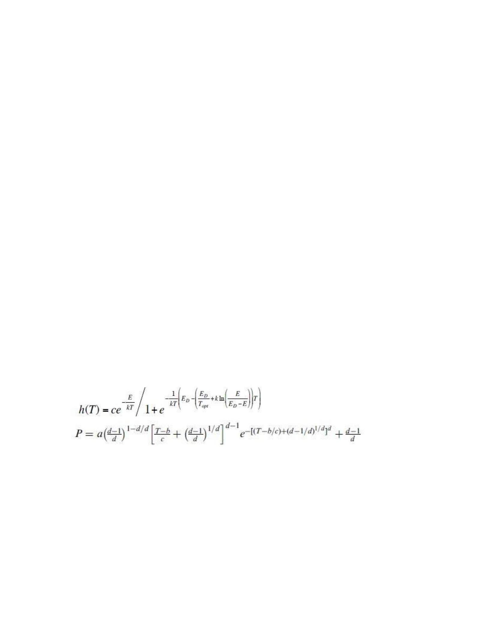
62
over the course of up to four consecutive months and did not use data collected over longer
periods of time, requiring us to average climate data over multiple seasons, which we deemed too
coarse of a climate measurement for our analysis.
Statistical Analyses
For the Host Temperature Preference Experiment, differences in temperature preferences
among the three species were assessed using a one-way ANOVA followed by Tukey’s posthoc
multiple comparison tests (stats package, aov and TukeyHSD functions, assuming normal error
distributions). In the Chytrid Growth Experiments, we fit a logistic growth model to mean Bd
optical density or zoospore counts at each time point within each temperature treatment
[assuming no growth at t0; bbmle package (Bolker 2014), mle2 function, negative log-likelihood
function, assuming a normal error distribution] to quantify Bd growth in culture. We then fit
Johnson-Lewin [Equation 1; (Dell, Pawar et al. 2011)] and Weibull [Equation 2; (Angilletta Jr
2006)] growth models to Bd growth rates (r parameter from logistic growth fits) across
temperatures [bbmle package (Bolker 2014), mle2 function, assuming a normal error
distribution].
(1)
(2)
These models are capable of producing asymmetrical temperature-performance curves
that do not fall below zero on the y-axis. They also produce parameter estimates for temperature
of peak growth (Topt in Johnson-Lewin; b in Weibull) based on a negative log-likelihood function.
To determine peak Bd growth of each isolate, we compared the AICs of both models and chose
the peak growth parameter of the better performing model. We also fit these models to previously
published data describing temperature-dependent Bd growth in culture (Piotrowski et al 2004,

63
Woodhams et al 2008) and compared the temperatures of peak growth across the isolates (Fig.
C3). For all isolates, we assumed zero growth at 0° and 32°C. To estimate 95% confidence
intervals for our parameters, we profiled all models fit using mle2 (profile function, stats
package).
To analyze Bd growth on frogs in the Chytrid Growth Experiments, we fit a logistic
growth model to each individual’s log Bd load over time, after adjusting all Bd loads for body size
by dividing by mass because larger frogs are swabbed over a larger area [bbmle package (Bolker
2014), mle2 function, normal error distribution]. If an animal died during the experiment, we still
fit a logistic growth model if the animal had at least three data points (meaning it was swabbed at
least twice because we assumed zero growth at t0). We then extracted the growth rate parameter, r,
from each fit and averaged parameters within temperature treatments and species. We competed
linear, exponential, Johnson-Lewin, and Weibull growth models to the fits of Bd growth rates, r,
across temperatures, using the model with the lowest AIC.
Given that the thermal mismatch hypothesis posits that the temperature of peak prevalence
for warm- and cold-adapted species should be at relatively cool and warm temperatures,
respectively, it required that we fit thermal performance curves separately to warm- and
coldadapted populations in our Field Study and estimate the temperature of maximum prevalence.
Hence, this required that we utilize a “reaction-norm” approach fitting Weibull models to the
prevalence data of warm- and cold-adapted populations as a function of the 50 year mean of each
population’s environmental temperature [bbmle package (Bolker 2014), mle2 function]. These
models utilized a binomial error distribution and took into account the number of frogs swabbed
in each population. To assign populations of frogs as either warm- or cold-adapted, we identified
the median environmental temperature of all populations as 17.5°C and then split the data into

64
cool-adapted host species that had annual 50 year mean environmental temperatures <15°C and
warm-adapted host species that had annual 50 year mean environmental temperatures of >20°C.
Lastly, we also fit models with precipitation as a linear covariate alongside temperature. We
restricted these field analyses to samples from adult amphibian populations with at least five
amphibians sampled, yielding 60,245 animals from 2,170 populations surveyed.
Results
Host Temperature Preference Experiment
Mean temperature preferences of An. terrestris (mean ± 1 SE: 24.07 ± 0.19°C) and O.
septentrionalis (22.98 ± 0.53°C) did not differ significantly (Tukey’s HSD, p = 0.12) but both
species preferred significantly warmer temperatures than At. zeteki (17.85 ± 0.14°C; Tukey’s
HSD, p < 0.0001 for both pairs of species; Fig. 4.2; Table C1), supporting the hypothesis that An.
terrestris and O. septentrionalis are relatively warm-adapted hosts and At. zeteki is a relatively
cold-adapted host.
Chytrid Growth Experiments
Incubators consistently maintained temperatures within ± 0.5°C of targets throughout all
trials (Fig. C4). We fit non-linear unimodal Johnson-Lewin models to Bd growth in culture
because these fits had lower AICs than Weibull, linear or exponential fits. In all experiments, the
temperature-dependent curve describing Bd growth in culture closely followed previously
reported patterns (Piotrowski, Annis et al. 2004; Woodhams, Alford et al. 2008), slowly rising
from 5°C until peaking around 20°C before quickly crashing around 26°C (Fig. 4.3; Fig. C3).
Isolate JEL423 from Panama peaked in growth at 18.0°C (95% confidence interval 17.1-18.9°C)
and isolate SRS812 from the southeastern US peaked at 18.9°C (95% CI 18.1-19.6°C). Thus, the
two isolates did not differ significantly in their optimum growth temperatures. Additionally, both

65
of the Bd isolates we tested were capable of exhibiting reasonably high growth rates (50% of
maximum) between 10° and 25°C, supporting the notion that Bd has a reasonably large breadth.
We fit linear or exponential models to Bd growth on frogs because these fits had lower
AICs than the unimodal fits. Without extrapolation beyond the tested temperatures, peak Bd
growth rates were predicted to be at 10°C on An. terrestris and 14°C on O. septentrionalis, which
are much lower temperatures than 18.9°C, the temperature of peak Bd growth in culture (Fig.
4.3a). We observed very little mortality among these two species (two and three total deaths, or
between 6-10% mortality). In contrast to the results for the warm-adapted species, Bd growth
rates on the cold-adapted At. zeteki were positively, not negatively, associated with temperature
(Fig. 4.3b), peaking at warmer temperatures than those where Bd grew best in culture. The
greatest Bd growth for At. zeteki occurred at 26°C, whereas peak Bd growth in culture for this
isolate occurred at 18.0°C (Fig. 4.3b).
Field Study
On average, peak Bd prevalence occurred under conditions only slightly cooler than those
that promoted peak growth in culture (17.0°C, 95% CI 16.4-17.4°C) (Fig. C5; Table C1).
However, amphibian populations from cool climates (averaging <15°C) experienced peak Bd
prevalence at 20.5°C (95% CI 19.6-22.1°C; Fig. 4.4a). This was significantly higher (i.e., 95%
CI did not overlap) than the temperature of peak Bd prevalence for amphibians from warm
climates (>20°C), which was only 15.9°C (95% CI 15.4-16.4°C; Fig. 4.4b), a result consistent
with the predictions of the thermal mismatch hypothesis. Also consistent with the thermal
mismatch hypothesis (see Fig. 1c,d), the thermal performance curve of Bd growth on amphibian
populations from cool climates was left skewed (Fig. 4a), whereas the curve for populations from
warm climates was right skewed (Fig. 4b). Including precipitation in multivariate models with
temperature did not improve fits of models predicting Bd outbreaks.

66
Discussion
Hosts are likely to experience thermal stress at unusual temperatures (Raffel, Rohr et al.
2006) and microbes and pathogens are known to have broad geographic ranges and thermal
breadths (the Baas Becking Hypothesis, Baas-Becking 1934; Rohr, Civitello et al. in review).
Therefore, we hypothesized that species adapted to warm conditions would experience high Bd
loads at cooler temperatures than host species adapted to cool conditions, which should
experience high Bd loads at relatively warm temperatures. We also hypothesized that parasite
prevalence on cold- and warm-adapted hosts as a function of temperature should be left and right
skewed, respectively (Fig. 1c,d). As hypothesized, O. septentrionalis and An. terrestris, species
from relatively warm climates that preferred higher temperatures (23-24°C) in our thermal
preference trials, suffered the highest Bd loads at colder temperatures than Bd’s optimal growth
temperature in culture. Meanwhile, At. zeteki, a cool, montane species that preferred cooler
temperatures (17.8°C), experienced rapid Bd growth at warmer temperatures than those where Bd
grew well in culture. Likewise, our analysis of Bd outbreaks in the field revealed that species
adapted to cool conditions experienced peak Bd prevalence at warmer temperatures than
warmadapted species. Also as hypothesized, the relationship between environmental temperature
and parasite prevalence for cold- and warm-adapted hosts in the field was left and right skewed,
respectively (Fig. 4.4).
Our experimental and field results broadly support the thermal mismatch hypothesis,
suggesting that host species are more susceptible to disease at temperatures far from those to
which they are adapted. In a recent article, Nowakowski et al. (2016) suggested that another
dimension of thermal mismatch, the gap between upper critical thermal tolerances (CTmax) of
amphibian hosts and Bd, is negatively related to disease risk. Nowakowski et al. estimated this

67
mismatch in thermal tolerance by calculating the difference between hosts and an assumed
constant CTmax for Bd worldwide. There is evidence, however, for local adaptation of Bd isolates
to environmental conditions (Stevenson, Alford et al. 2013). Thus, by subtracting a constant from
the CTmax of every host, these estimates of thermal mismatch are confounded with host thermal
tolerance. In addition, this study did not address the disparity between thermal breadths of hosts
and parasites or consider how the host-parasite interaction might differ from host or parasite
performance (CTmax) in isolation. Our findings address these concepts as well as the fact that
Bdrelated declines often happen in particularly warm years (Rohr, Raffel et al. 2008; Rohr and
Raffel 2010).
Although the thermal mismatch hypothesis was supported by our findings in a system with
pathogens that have free-living stages and ectothermic hosts, questions remain about the
generality of the hypothesis across systems. For example, disease susceptibility is less
temperature-dependent for endotherms than ectotherms (Harvell, Mitchell et al. 2002; Martin,
Hopkins et al. 2010; Altizer, Ostfeld et al. 2013). In addition, parasites that lack free-living stages,
such as vector-borne pathogens, may also be less directly affected by environmental conditions
(Harvell, Mitchell et al. 2002; Altizer, Ostfeld et al. 2013), although traits of some vectors can
profoundly depend on temperature (Mordecai, Paaijmans et al. 2013; Johnson, BenHorin et al.
2015). We expect that the thermal mismatch hypothesis most likely applies to cases of
ectothermic hosts and pathogens with free-living stages, but there is a need to test this hypothesis
across systems and pathogens. Additionally, in cases where the thermal breadth of the pathogen is
narrower than that of the host, extreme temperatures could provide a refuge for hosts (Gsell,
Domis et al. 2013), although such cases may be uncommon (Rohr, Civitello et al. in review).
Several of our observations might resolve uncertainties regarding how environmental
temperature impacts Bd outbreaks in the field (Venesky, Raffel et al. 2014). In contrast with the

68
considerable variability among hosts in their temperature-dependent susceptibility to Bd, we
observed much less variation in optimal growth temperatures among Bd isolates grown in culture
(including two that have been previously reported; Piotrowski, Annis et al. 2004; Woodhams,
Alford et al. 2008). Importantly, temperature-dependent Bd growth in culture would have poorly
predicted temperature-dependent host susceptibility for all species we tested (Rohr, Raffel et al.
2008), even though models predicting Bd distributions are often parameterized based on growth
in culture (Pounds, Bustamante et al. 2006; Rohr, Raffel et al. 2008; Woodhams, Alford et al.
2008; Murray, Skerratt et al. 2013). Surprisingly, Bd growth patterns on animals were linearly or
exponentially related to temperature, implying that poor host resistance can encourage pathogen
growth even at extreme conditions where pathogens do relatively poorly in culture. We observed
large infection loads for At. zeteki at high temperatures (26-28°C), contrasting the observed
pattern of Bd growth in culture and suggesting that Bd has the potential to cause outbreaks well
outside of the conditions where it traditionally has been thought to flourish. These results
highlight the need to either explicitly consider the host-parasite interaction or evaluate the
difference in host and parasite performance in isolation rather than only one of their performances
alone.
Much of the recent debate over whether global climate change is likely to increase the
spread of disease focuses on how changing climates will impact pathogen ranges (Epstein 2001;
Lafferty 2009; Murray, Retallick et al. 2011), with fewer papers exploring the effect of climatic
shifts on host immunity or resistance (Martin, Hopkins et al. 2010; Rohr, Dobson et al. 2011). In
general, parasites might be more adaptable to climate change than their hosts because of their
shorter generation times and faster acclimation rates (Raffel, Romansic et al. 2013; Rohr,
Civitello et al. in review). Warmer mean temperatures are likely to push hosts away from their
optimal temperatures and result in greater thermal mismatches between hosts and parasites,

69
particularly for cold-adapted hosts. Meanwhile, sudden temperature drops that occur following
warm periods (Rohr and Raffel 2010) may cause thermal mismatches between warm-adapted
hosts and their parasites. In addition, extreme weather events are likely to increase with climate
change (Rosenzweig, Iglesias et al. 2001), exposing hosts to unusual temperatures and lending
pathogens an advantage in host-parasite interactions. To manage outbreaks, it will be critical that
researchers account for thermal mismatches between the performance of hosts and parasites when
predicting temperature-dependent disease outcomes across systems.
Acknowledgments
We want to thank the Maryland Zoo for providing us with At. zeteki used in the experiments. We
thank N. Argento, H. Folse, C. Gionet, T. James, C. Koshy, C. Malave, L. Martinez-Rodriguez, C.
Steffan, S. Rubano, and K. Vazquez for their assistance in all aspects of the lab work and
maintenance of experiments. In addition, we thank B. Delius, S. Knutie, K. Nguyen, N. Ortega,
D. Pike, C. Ramsay, and S. Young for their helpful comments on the manuscript and collection of
data for the field analyses. Funds were provided by grants to J.R.R. from the National Science
Foundation (EF-1241889 and DEB-1518681), the National Institutes of Health (R01GM109499,
R01TW010286-01), the US Department of Agriculture (2009-35102-0543), and the US
Environmental Protection Agency (CAREER 83518801). Funds were also provided from the
University of Tampa (Faculty Development Dana Grant) to T.A.M.

70
Figures
Figure 4.1. Conceptual figure describing the thermal mismatch hypothesis. In isolation, small
organisms, such as parasites (dashed lines in panels a and b), generally have broader performance
breadths than larger organisms, such as hosts (solid lines in panels a and b). Thus, highest
parasite growth on hosts is likely to occur at a temperature where a parasite most outperforms its
host (bidirectional arrows), and not necessarily at the temperature which a parasite performs best
in isolation. Hence, subtracting the thermal performance curves of hosts and parasites reared in
isolation (panels a and b) provides a hypothesis for the thermal performance curve of a parasite
growing on the host (panels c and d). For interacting coldadapted hosts and parasites, this
subtraction reveals that parasite growth should be maximized at relatively warm temperatures (a
and c) and the performance curve should be left skewed (c). In contrast, for interacting warm-
adapted hosts and parasites, parasite growth should be maximized at relatively cool temperatures
(b and d) and the performance curve should be right skewed (d). Thus, even when hosts and
parasites have identical optimum performance temperatures because of local adaptation (although
they could differ), small breadth differences in temperatureperformance patterns can cause peak
growth to occur far from the conditions under which the parasite or host perform best in isolation.

71
Figure 4.2. Mean (± 1 SE) temperature preferences of amphibian host species. To ascertain
temperature preferences, we maintained uninfected Anaxyrus terrestris, Osteopilus
septentrionalis, and Atelopus zeteki (n = 24, 25, and 9, respectively) in thermal gradient
apparatuses containing temperature gradients ranging from 8-33°C.
Figure 4.3. Temperature-dependent growth of Bd on hosts versus in culture is consistent
with the thermal mismatch hypothesis. In all three species, growth of Bd on the host differed
from growth in culture. a) Bd growth rates on Anaxyrus terrestris (solid triangles) and Osteopilus
septentrionalis (solid squares) were highest at cold temperatures (10 and 14°C, respectively,
based on linear fits), despite Bd growth in culture peaking at 18.9°C (solid circles, JohnsonLewin
fit; 95% confidence interval 18.1-19.6°C). b) At. zeteki experienced high Bd growth (exponential
fit) at warm temperatures (open squares; combined results of two temporal blocks), even though

72
Bd growth in culture was poor at these temperatures, peaking at 18.0°C (open circles, Johnson-
Lewin fit; 95% confidence interval 17.1-18.9°C). We could not measure Bd growth rates on At.
zeteki at 28°C because too few animals survived long enough to be tested multiple times, which is
necessary to fit the logistic growth curves. Shown are means ± 1 SE.
Figure 4.4. Temperature-dependence of peak Bd prevalence varies between cold- and warm-
tolerant host species in a manner that is consistent with the thermal mismatch hypothesis.
Amphibian populations were divided into a) cold- (<15°C) and b) warm-adapted (>20°C) based
on their 50-year mean annual temperatures. Separately for both the cold- and warm-adapted
groups, Weibull models were fit to the relationship between Bd prevalence in adult amphibians (n
≥5 animals) and temperature at the specific sampling location during the months of field
sampling. Populations from cool climates experienced peak Bd prevalence at relatively warm
temperatures (20.5°C; 95% confidence interval 19.6-22.1°C), where populations from warm
climates experienced peak prevalence at cooler temperatures (15.9°C; 95% CI 15.416.4°C),
providing support for the thermal mismatch hypothesis.
References
Altizer, S., R. S. Ostfeld, et al. (2013). "Climate Change and Infectious Diseases: From Evidence
to a Predictive Framework." Science 341(6145): 514-519.
Anderson, P. K., A. A. Cunningham, et al. (2004). "Emerging infectious diseases of plants:
pathogen pollution, climate change and agrotechnology drivers." Trends in Ecology &
Evolution 19(10): 535-544.
Angilletta Jr, M. J. (2006). "Estimating and comparing thermal performance curves." Journal of

73
Thermal Biology 31(7): 541-545.
Anyamba, A., J. L. Small, et al. (2014). "Recent weather extremes and impacts on agricultural
production and vector-borne disease outbreak patterns." PLoS ONE 9(3): e92538.
Baas-Becking, L. G. M. (1934). Geobiologie; of inleiding tot de milieukunde, WP Van Stockum
& Zoon NV.
Bolker, B. (2014). "bbmle: Tools for general maximum likelihood estimation, R package version
1.0.16."
Bosch, J., L. M. Carrascal, et al. (2007). "Climate change and outbreaks of amphibian
chytridiomycosis in a montane area of Central Spain; is there a link?" Proceedings of the
Royal Society B-Biological Sciences 274(1607): 253-260.
Boyle, D. G., D. B. Boyle, et al. (2004). "Rapid quantitative detection of chytridiomycosis
(Batrachochytrium dendrobatidis) in amphibian samples using real-time Taqman PCR
assay." Diseases of Aquatic Organisms 60(2): 141-148.
Bruno, J. F., E. R. Selig, et al. (2007). "Thermal stress and coral cover as drivers of coral disease
outbreaks." Plos Biology 5(6): 1220-1227.
Cazelles, B., M. Chavez, et al. (2005). "Nonstationary influence of El Nino on the synchronous
dengue epidemics in Thailand." Plos Medicine 2(4): 313-318.
Cohen, J. M., D. J. Civitello, et al. (2016). "Spatial scale modulates the strength of ecological
processes driving disease distributions." Proceedings of the National Academy of
Sciences of the United States of America 113(24): E3359-E3364.
Daszak, P. (2000). "Emerging infectious diseases of wildlife - Threats to biodiversity and human
health (vol 287, pg 443, 2000)." Science 287(5459): 1756-1756.

74
Dell, A. I., S. Pawar, et al. (2011). "Systematic variation in the temperature dependence of
physiological and ecological traits." Proceedings of the National Academy of Sciences of
the United States of America 108(26): 10591-10596.
Epstein, P. R. (2001). "Climate change and emerging infectious diseases." Microbes and Infection
3(9): 747-754.
Fisher, M. C., D. A. Henk, et al. (2012). "Emerging fungal threats to animal, plant and ecosystem
health." Nature 484(7393): 186-194.
Fitt, W. K., R. D. Gates, et al. (2009). "Response of two species of Indo-Pacific corals, Porites
cylindrica and Stylophora pistillata, to short-term thermal stress: The host does matter in
determining the tolerance of corals to bleaching." Journal of Experimental Marine Biology
and Ecology 373(2): 102-110.
Frost, D. R. (2015). "Amphibian Species of the World: An Online Reference. Version 6.0.
Accessible at http://research.amnh.org/herpetology/amphibia/index.html. American
Museum of Natural History, New York, USA."
Gsell, A. S., L. N. D. Domis, et al. (2013). "Temperature Alters Host Genotype-Specific
Susceptibility to Chytrid Infection." PLoS ONE 8(8).
Harris, I., P. D. Jones, et al. (2014). "Updated high-resolution grids of monthly climatic
observations - the CRU TS3.10 Dataset." International Journal of Climatology 34(3):
623642.
Harvell, C. D., C. E. Mitchell, et al. (2002). "Ecology - Climate warming and disease risks for
terrestrial and marine biota." Science 296(5576): 2158-2162.
Hijmans, R. J. (2014). "raster: Geographic data analysis and modeling, R package version
2.2.31."

75
IUCN (2015). "The IUCN Red List of Threatened Species. Version 2015.2. Accessible at
www.iucnredlist.org."
Johnson, L. R., T. Ben-Horin, et al. (2015). "Understanding uncertainty in temperature effects on
vector‐borne disease: a Bayesian approach." Ecology 96(1): 203-213.
Jones, K. E., N. G. Patel, et al. (2008). "Global trends in emerging infectious diseases." Nature
451(7181): 990-U994.
Kilpatrick, A. M., C. J. Briggs, et al. (2010). "The ecology and impact of chytridiomycosis: an
emerging disease of amphibians." Trends in Ecology & Evolution 25(2): 109-118.
Koelle, K., X. Rodo, et al. (2005). "Refractory periods and climate forcing in cholera dynamics."
Nature 436(7051): 696-700.
Kriger, K. M. and J. M. Hero (2007). "The chytrid fungus Batrachochytrium dendrobatidis is non-
randomly distributed across amphibian breeding habitats." Diversity and
Distributions 13(6): 781-788.
Kriger, K. M. and J. M. Hero (2007). "Large-scale seasonal variation in the prevalence and
severity of chytridiomycosis." Journal of Zoology 271(3): 352-359.
Lafferty, K. D. (2009). "The ecology of climate change and infectious diseases." Ecology 90(4):
888-900.
Laine, A. L. (2008). "Temperature-mediated patterns of local adaptation in a natural
plantpathogen metapopulation." Ecology Letters 11(4): 327-337.
Lampo, M., A. Rodriguez-Contreras, et al. (2006). "A chytridiomycosis epidemic and a severe dry
season precede the disappearance of Atelopus species from the Venezuelan Andes."
Herpetological Journal 16(4): 395-402.
Laurance, W. F. (2008). "Global warming and amphibian extinctions in eastern Australia."
Austral Ecology 33(1): 1-9.

76
Liu, X., J. R. Rohr, et al. (2013). "Climate, vegetation, introduced hosts and trade shape a global
wildlife pandemic." Proceedings of the Royal Society B-Biological Sciences 280(1753).
Martin, L. B., W. A. Hopkins, et al. (2010). "The effects of anthropogenic global changes on
immune functions and disease resistance." Year in Ecology and Conservation Biology
2010 1195: 129-148.
McMahon, T. A. and J. R. Rohr (2014). "Trypan Blue Dye is an Effective and Inexpensive Way to
Determine the Viability of Batrachochytrium dendrobatidis Zoospores." Ecohealth 11(2):
164-167.
McMahon, T. A., J. M. Romansic, et al. (2013). "Nonmonotonic and Monotonic Effects of
Pesticides on the Pathogenic Fungus Batrachochytrium dendrobatidis in Culture and on
Tadpoles." Environmental Science & Technology 47(14): 7958-7964.
Mordecai, E. A., K. P. Paaijmans, et al. (2013). "Optimal temperature for malaria transmission is
dramatically lower than previously predicted." Ecology Letters 16(1): 22-30.
Murray, K. A., R. W. R. Retallick, et al. (2011). "Assessing spatial patterns of disease risk to
biodiversity: implications for the management of the amphibian pathogen,
Batrachochytrium dendrobatidis." Journal of Applied Ecology 48(1): 163-173.
Murray, K. A., L. F. Skerratt, et al. (2013). "Whether the Weather Drives Patterns of Endemic
Amphibian Chytridiomycosis: A Pathogen Proliferation Approach." PLoS ONE 8(4).
Nowakowski, A. J., S. M. Whitfield, et al. (2016). "Infection risk decreases with increasing
mismatch in host and pathogen environmental tolerances." Ecology Letters.
Pascual, M., B. Cazelles, et al. (2008). "Shifting patterns: malaria dynamics and rainfall
variability in an African highland." Proceedings of the Royal Society B-Biological
Sciences 275(1631): 123-132.

77
Piotrowski, J. S., S. L. Annis, et al. (2004). "Physiology of Batrachochytrium dendrobatidis, a
chytrid pathogen of amphibians." Mycologia 96(1): 9-15.
Pounds, J. A., M. R. Bustamante, et al. (2006). "Widespread amphibian extinctions from epidemic
disease driven by global warming." Nature 439(7073): 161-167.
Puschendorf, R., A. C. Carnaval, et al. (2009). "Distribution models for the amphibian chytrid
Batrachochytrium dendrobatidis in Costa Rica: proposing climatic refuges as a
conservation tool." Diversity and Distributions 15(3): 401-408.
Raffel, T. R., J. R. Rohr, et al. (2006). "Negative effects of changing temperature on amphibian
immunity under field conditions." Functional Ecology 20(5): 819-828.
Raffel, T. R., J. M. Romansic, et al. (2013). "Disease and thermal acclimation in a more variable
and unpredictable climate." Nature Climate Change 3(2): 146-151.
Retallick, R. W. R., H. McCallum, et al. (2004). "Endemic infection of the amphibian chytrid
fungus in a frog community post-decline." Plos Biology 2(11): 1965-1971.
Rohr, J., D. J. Civitello, et al. (in review). "A global framework for estimating acclimation and
thermal breadth predicts risk from climate change " Proceedings of the National Academy
of Sciences of the United States of America.
Rohr, J. R., A. P. Dobson, et al. (2011). "Frontiers in climate change-disease research." Trends in
Ecology & Evolution 26(6): 270-277.
Rohr, J. R. and T. R. Raffel (2010). "Linking global climate and temperature variability to
widespread amphibian declines putatively caused by disease." Proceedings of the National
Academy of Sciences of the United States of America 107(18): 8269-8274.
Rohr, J. R., T. R. Raffel, et al. (2008). "Evaluating the links between climate, disease spread, and
amphibian declines." Proceedings of the National Academy of Sciences of the United
States of America 105(45): 17436-17441.

78
Ron, S. R., W. E. Duellman, et al. (2003). "Population decline of the Jambato Toad Atelopus
ignescens (Anura : Bufonidae) in the Andes of Ecuador." Journal of Herpetology 37(1):
116-126.
Rosenzweig, C., A. Iglesias, et al. (2001). "Climate change and extreme weather events;
implications for food production, plant diseases, and pests." Global change & human
health 2(2): 90-104.
Rowley, J. J. and R. A. Alford (2007). "Non-contact infrared thermometers can accurately
measure amphibian body temperatures." Herpetological Review 38: 308-316.
Sauer, E., J. Sperry, et al. (2016). "An efficient and inexpensive method for measuring long-term
thermoreulatory behavior of terrestrial and semi-terrestrial organisms." Thermal Biology
60: 231-236.
Skerratt, L. F., L. Berger, et al. (2007). "Spread of chytridiomycosis has caused the rapid global
decline and extinction of frogs." Ecohealth 4(2): 125-134.
Sodhi, N. S., D. Bickford, et al. (2008). "Measuring the Meltdown: Drivers of Global Amphibian
Extinction and Decline." PLoS ONE 3(2).
Sternberg, E. D. and M. B. Thomas (2014). "Local adaptation to temperature and the implications
for vector-borne diseases." Trends in Parasitology 30(3): 115-122.
Stevenson, L. A., R. A. Alford, et al. (2013). "Variation in Thermal Performance of a Widespread
Pathogen, the Amphibian Chytrid Fungus Batrachochytrium dendrobatidis." PLoS ONE
8(9).
Team, R. C. (2014). R: A language and environment for statistical computing. R Foundation for
Statistical Computing, Vienna, Austria.
Thomas, M. B. and S. Blanford (2003). "Thermal biology in insect-parasite interactions." Trends
in Ecology & Evolution 18(7): 344-350.

79
Venesky, M. D., T. R. Raffel, et al. (2014). "Confronting inconsistencies in the
amphibianchytridiomycosis system: implications for disease management." Biological
Reviews 89(2): 477-483.
Whitfield, S. M., J. Kerby, et al. (2012). "Temporal Variation in Infection Prevalence by the
Amphibian Chytrid Fungus in Three Species of Frogs at La Selva, Costa Rica." Biotropica
44(6): 779-784.
Woodhams, D. C., R. A. Alford, et al. (2008). "Life-history trade-offs influence disease in
changing climates: strategies of an amphibian pathogen." Ecology 89(6): 1627-1639.
CHAPTER FIVE:
AN INTERACTION BETWEEN CLIMATE CHANGE AND INFECTIOUS DISEASE
DROVE WIDESPREAD AMPHIBIAN EXTINCTIONS
Authors
Jeremy M. Cohen, Matthew D. Venesky, David J. Civitello12, Taegan A. McMahon, Jason
R. Rohr12

80
Abstract
Infectious disease outbreaks are increasing while global temperatures are simultaneously rising;
however, whether climate change is responsible for the increase in disease outbreaks is
controversial. Although models have predicted that climate change could be responsible for
increases in the frequency and intensity of disease, we lack experiments and field data that
together support a causal link between climate change and disease-mediated extinctions. Thus, we
have little concrete evidence of an interaction between disease and climate change causing
widespread declines. Here, we examined whether climate change may have contributed to a
widespread extinction event in the amphibian genus Atelopus, putatively caused by the fungal
pathogen Batrachochytrium dendrobatidis (Bd). We experimentally tested the susceptibility of A.
zeteki to Bd across a temperature spectrum and examined trends in historic climate data
corresponding to species extinctions. We found that A. zeteki experienced high and rapid
mortality as a result of an interaction between Bd exposure and high temperatures (26-28°C),
while Bd growth peaked at 20°C in isolation. Further, when historic climate data in Atelopus spp.
ranges was parameterized using the experimental results, the pattern describing
temperaturedependent A. zeteki mortality was much more predictive of the conditions preceding
declines than the pattern describing Bd growth in culture. Finally, conditions experienced by
Atelopus spp. leading up to extinction were significantly warmer than both conditions they had
experienced historically and conditions simultaneously experienced by species that remained
extant. By combining experiments with field data, we provide evidence that one of the greatest
mass extinction events in recent times may have been caused by an interaction between climate
change and emerging infectious disease.

81
Main Text
Global climate change and emerging infectious diseases represent two of the most
formidable ecological challenges in modern times, but controversy exists over whether they are
causally linked (Harvell, Mitchell et al. 2002; Lafferty 2009; Rohr, Dobson et al. 2011). Climatic
conditions often directly influence outbreaks of disease (Stenseth, Mysterud et al. 2002; Pascual,
Chaves et al. 2008), and climate-related shifts in biotic interactions have been indirectly
associated with extinctions (Cahill, Aiello-Lammens et al. 2013). In addition, many predictive
models have suggested that climate change could be responsible for future increases in the
intensity and frequency of disease outbreaks (Patz, Campbell-Lendrum et al. 2005; Ermert, Fink
et al. 2012; Liu, Rohr et al. 2013). However, we have surprisingly little concrete evidence of
interactions between climate change and disease causing widespread species declines (Rohr,
Dobson et al. 2011).
There may be several reasons why evidence is lacking. First, many climate change studies
do not adequately address the fact that climate change occurs heterogeneously in space and time;
thus, we lack studies testing hypotheses using precise climate data, such as data specific to
species’ ranges and years preceding extinction. Second, models predicting outbreaks of infectious
diseases are often parameterized based only on temperature-dependent parasite growth in
isolation rather than growth on the host (Harvell, Mitchell et al. 2002; Rodder, Kielgast et al.
2010; Rohr and Raffel 2010; Maher, Kramer et al. 2012; Cohen, Venesky et al. in prep), which
may cause them to associate incorrect climatic conditions with disease outbreaks. Finally, we lack
experiments, field data, and demographic models that together support a causal link between
climate change and extinctions mediated by disease (Rohr, Dobson et al. 2011).
A number of high profile papers have recently debated links between climate change,
outbreaks of the pathogenic chytrid fungus Batrachochytrium dendrobatidis (Bd), and amphibian

82
declines, using the genus Atelopus as a case study (e.g., (Pounds, Bustamante et al. 2006; Lips,
Diffendorfer et al. 2008; Rohr, Raffel et al. 2008; Rohr and Raffel 2010). Bd, generally
considered to be one of the deadliest emerging wildlife pathogens (Skerratt, Berger et al. 2007;
Collins 2013), is linked to 50-80 extinctions within Atelopus (La Marca, Lips et al. 2005). The
debate primarily centered around correlative relationships between historic climate trends and
Atelopus spp. extinctions using a dataset published by La Marca et al. (2005) documenting the
last year each Atelopus species was observed in the wild, which is perhaps the most
comprehensive spatiotemporal dataset describing a modern mass extinction. Although Bd
outbreaks have long been expected to occur under cool or moderate conditions (16-24°C) based
on the temperature-dependent growth pattern of Bd in culture (Kilpatrick, Briggs et al. 2010),
comparisons between the Atelopus spp. extinctions and historic climate data surprisingly revealed
an association between outbreaks and warm or highly variable temperatures (Pounds, Bustamante
et al. 2006; Rohr and Raffel 2010). However, these analyses used global and regional climate data
instead of data specific to species’ ranges, and neither tested the response of Atelopus spp. to Bd
under controlled conditions. Thus, we do not have clear, causal evidence of the precise climatic
conditions that enabled Bd outbreaks and caused a mass extinction event.
We hypothesized that warm temperatures and Bd interact to increase Atelopus spp.
mortality, because throughout geologic time, Atelopus spp. experienced variable climates and
persisted, but began declining once Bd arrived and conditions warmed. Additionally, we expected
that the temperature-dependent pattern of Bd-induced Atelopus mortality would be more
predictive of extinctions than the pattern of Bd growth in culture across temperatures. To test our
hypotheses, we grew Bd in culture and exposed Atelopus zeteki (acquired from the Maryland Zoo
in Baltimore, MD), a species considered to have life history characteristics relatively similar to
the rest of the genus (Karraker, Richards et al. 2006) to Bd across a temperature gradient (14°,

83
18°, 22°, 26°, and 28°C) in two temporal blocks (Figs. D1, D2). We then parameterized predictive
models of Bd-associated Atelopus extinctions based on the observed temperaturedependent
patterns of both Bd growth in culture and A. zeteki mortality. In addition, we collected historic
monthly temperature records for the geographic ranges of each Atelopus species, predicting that
climate change in each species’ range would have been greatest in the years before each
extinction, and that more climate change would have occurred in extinct than extant species’
ranges. Finally, we incorporated the temperature-dependent increase in disease-related mortality
revealed by our experiments into a demographic model, which we predicted would account for
the observed Atelopus spp. extinctions. By linking experiments, models, and analyses of field
data, our primary goal was to establish a more definitive causal link between climate, disease
outbreaks and widespread extinctions.
There was no relationship between temperature and mortality when A. zeteki was not
exposed to Bd (cox proportional hazards model; X2=0.54, p=0.46), but mortality increased
significantly with temperature when A. zeteki was exposed to Bd (Bd x temperature: X2=4.41,
p=0.036). In fact, within five days of exposure to Bd, the 26° and 28° treatments experienced
69% and 78% mortality respectively, while only one animal died among the coldest treatments
(Fig. 5.1b). This suggests a cost of exposure to Bd. Similarly, Bd growth rates on frogs increased
significantly with increasing temperatures (Fig. 5.1a). In contrast, Bd growth in culture across
temperatures closely followed previously reported patterns, peaking at approximately 20°C and
declining at both cooler and warmer temperatures (Piotrowski, Annis et al. 2004; Woodhams,
Alford et al. 2008) (Fig. 5.1a). We observed similar A. zeteki mortality and Bd growth patterns
during both temporal blocks (Fig. D3).

84
To parameterize Atelopus spp. extinction models, we extracted the linear equation from
the temperature-dependent Atelopus mortality pattern and the unimodal equation describing Bd
growth in culture (Fig. 5.1a). We used these equations to generate mortality probabilities as a
proxy for extinction risk based on annual (1979-1998) temperatures averaged across the
geographic ranges of each Atelopus spp. While regional and even global climate data have been
used to predict Atelopus extinctions in previous analyses (Pounds, Bustamante et al. 2006; Rohr
and Raffel 2010), we suspected that these may be inappropriate spatial scales for predictors in this
analysis, because the majority of Atelopus spp. live at high elevations that experience different
climatic conditions than the region as a whole (Fig. 5.2). We then compared annual mortality
probabilities to detrended annual extinction totals (based on year of decline (YOD) totals, see (La
Marca, Lips et al. 2005; Rohr and Raffel 2010)) with a one year lag. These analyses revealed that
A. zeteki mortality in the experiment was a significant positive predictor of extinctions (R2=0.33,
p=0.01; Fig.3; see Fig. S4 for model reparameterization using regional climate data), while Bd
growth in culture was a poor predictor (R2<0.001, p=0.98; Fig. 5.3).
Although the correlative extinction models corroborated our experimental observations,
we wished to further establish a causal link between climate change and the Atelopus spp.
extinctions by closely examining the conditions experienced by Atelopus spp. before they went
extinct. Thus, we tested whether the climatic conditions (mean temperature and precipitation;
moisture is required for Bd to grow (Raffel, Halstead et al. 2015)) preceding extinction for each of
the 46 extinct Atelopus spp. differed from typical historic conditions experienced by each extinct
species’ and conditions experienced simultaneously by species that did not go extinct (Table S1)
(see (Alford, Bradfield et al. 2007) for a similar approach using two species). As predicted, mean
temperatures in the year or five-year window before extinctions were significantly higher than the
respective means in the same ranges over 40 years (binomial mixedeffects model; year-prior,

85
X2=41.35, p<0.0001; five-year windows, X2=78.42, p<0.0001; Table D3). To compare climate
change between extinct and extant Atelopus spp. (as of 2000; n=20 extant species), we matched
each five-year temperature slope before extinction to the five-year temperature slope for the same
window of time for all extant species. Temperature increased ~2.5 times faster in the five years
before extinction for extinct compared to extant species (matched pairs test; F1,45=7.73, p<0.01;
Fig. 5.3; Table D4). Interestingly, although warm and dry conditions tend to co-occur, the rate of
increase in precipitation levels was also higher among extinct species in the same analysis
(F1,45=4.17, p<0.05; Fig. 5.3, Table D4), likely because Bd can only survive in moist conditions
and precipitation is considered to be a crucial ingredient in epidemics (Murray, Retallick et al.
2011; Raffel, Halstead et al. 2015). In summary, extinct species were experiencing warm
conditions both unusual to them and unlike those experienced by species that survived.
Thus, the patterns observed in our experiment, model reparameterization, analysis of
historic climate data in Atelopus spp. ranges, and demographic model combine to suggest that
increasing temperatures and the presence of disease interacted to cause rapid mortality and
extinctions in Atelopus spp. Despite the common assumption that outbreaks of Bd can only occur
at cool or intermediate temperatures, we observed a strong pattern of high and rapid mortality and
faster Bd growth at the warmest temperatures in our experiment. Our findings stress the
importance of considering the host-parasite interaction before making conclusions about the
conditions likely to promote outbreaks. Consideration of Bd performance in isolation would not
have been able to predict Atelopus spp. extinctions; instead, it was necessary to experimentally
test the temperature-dependent host-parasite interaction to predict these extinctions.
Given our experimental results, Bd may flourish well outside of conditions under which it
grows best in isolation, providing context to correlations between warm years and Atelopus spp.

86
extinctions found here and in previous studies (Pounds, Bustamante et al. 2006; Rohr and Raffel
2010). Importantly, if Atelopus spp. are directly harmed by an interaction between Bd and warm
temperatures and Bd outbreaks are already known to be heavily controlled by climatic conditions
(cite), it is unlikely that a widespread, multi-decadal Bd epidemic could have occurred without
some level of environmental influence, which is what was suggested by Lips et al. (2008). In
addition, our explanation for Atelopus spp. declines and extinctions is more parsimonious than
alternatives that have been proposed (e.g., warm temperatures increase cloud cover allowing Bd
to be incubated, (Pounds, Bustamante et al. 2006)). However, because warm conditions and
highly variable temperature tend to co-occur, especially under Latin American climate patterns
heavily influenced by El Niño, our results do not rule out temperature variability as a contributor
to Atelopus spp. extinctions as suggested by Rohr et al. (2010).
As global temperatures are warming and infectious diseases outbreaks are increasing,
these two crises have been repeatedly correlated by researchers, although strong causal evidence
that they interact to cause species declines has been lacking. Here, by linking extinction data with
experiments, parameterizing models using data derived from a temperature-dependent
hostparasite interaction, and using precise spatiotemporal climate data in models, we demonstrate
that Atelopus spp. suffer rapid mortality upon Bd infection at warm but not cool temperatures and
that
Atelopus spp. experienced warming in their ranges prior to extinction. Thus, we provide causal
evidence that one of the greatest modern day mass extinction events was likely driven by an
interaction between increasing temperatures and infectious disease.

87
Methods
Temperature-dependent Bd growth experiment
A. zeteki, the only Atelopus species available for research in the U.S., were obtained from
the Maryland Zoo in Baltimore, MD. We exposed A. zeteki (n=8/temperature) to 3.75x10⁵
zoospores of Panamanian Bd isolate JEL 423 across a temperature gradient (14°, 18°, 22°, 26°
and 28°C) after acclimating animals to these temperatures for four weeks. We acclimated the
animals so as not to confound exposure to a pathogen with exposure to a new temperature.
Animals were kept in temperature-controlled insulated Styrofoam incubators containing
thermostats and lined on the bottom with heat tape (Raffel, Romansic et al. 2013), with two
animals per incubator (Fig. S1). Incubators maintained temperatures to within ±0.5°C throughout
the experiment (Fig. S3). Animals were swabbed for infection at one, two and four weeks
postexposure or on date of death and quantitative PCR (Boyle, Boyle et al. 2004) was performed
on the swabs. We repeated this experiment twice because initially we did not expect the high
mortality we observed and did not have unexposed control frogs present; in the second temporal
block, four unexposed animals were also maintained at each temperature. Simultaneously, two Bd
cultures (3.75x10⁵ zoospores in 8ml 1% tryptone broth) were grown in each incubator and
measured at one and two weeks using a spectrophotometer. Logistic growth curves were fitted to
log-Bd loads on frogs across both temporal blocks as well as Bd optical densities over time (All
analyses were conducted in R 3.1.0 (2014) unless otherwise indicated; bbmle package (Bolker
2014), mle2 function, assuming a normal error distribution and using a negative log-likelihood
function). The mean r (growth rate) parameter was calculated for growth across all temperatures.
We then fit growth rates to temperature using either linear, Weibull (Angilletta Jr 2006) or
Johnson-Lewin models (Dell, Pawar et al. 2011) (see Appendix D; bbmle package (Bolker 2014),

88
mle2 function, same assumptions as above), depending on which had the lowest AIC. To examine
the relationship between frog mortality, Bd exposure, and temperature, we fit cox-proportional
hazards survival models with temperature and Bd exposure as either non-interacting or interacting
fixed effects (survival package (Therneau 2014), coxph function), conservatively assuming that
animals surviving the length of the experiment (28 days) would have died on day 29. Please see
Cohen et al. (in prep) for more detailed methods.
Parameterization of extinction models
We revisited the La Marca et al. (2005) Atelopus spp. extinction dataset (Latin America, approx.
1973-2004) to test whether the temperature-dependent patterns of Bd growth in culture and A.
zeteki mortality observed in the experiment predicted extinctions. We extracted the equations
describing the above patterns in the experiment and calculated extinction probabilities for each
Atelopus spp. each year given the monthly mean temperatures that year using either the annual
broad-scale regional mean temperature data used by Rohr et al. (2008) and Rohr and Raffel
(2010) or the annual mean temperature data specific to each species’ geographic range (Fig. 2).
Although regional and global climatic data have been used in past publications on this extinction
dataset (Pounds, Bustamante et al. 2006; Rohr, Raffel et al. 2008; Rohr and Raffel 2010), we
were concerned that large-scale regional data may be very different from local conditions for the
Atelopus species, many of which are restricted to small, isolated high-elevation sites. Range-level
temperature data was collected by individually extracting data (Climate Research Unit 3.1,
University of East Anglia (Harris, Jones et al. 2014); raster package (Hijmans 2014), extract
function) from 0.5°2 cells cropped to each IUCN Atelopus species range (raster package (Hijmans
2014), crop function). We fit linear regressions to analyze whether temperature-based extinction
probabilities predicted detrended extinctions (stats package, glm function, assuming a normal

89
error distribution), rather than raw extinction totals, because detrended extinctions can account
for the diminishing pool of potential host species as extinctions occur over time (Rohr and Raffel
2010). We restricted our analysis to 1980-1999, the same time period used by Rohr and Raffel
(2010).
Species-specific climatic signals before extinction
We extracted monthly mean temperature and precipitation (Hadley Climate Research Unit
TS 3.1 (Harris, Jones et al. 2014); raster package (Hijmans 2014), extract function) averaged
within the IUCN ranges of each of 46 extinct and 20 extant Atelopus species. “Extinct” species
included those that had an LYO between 1973-1999, and “extant” species were those with an
LYO within five years of the assessment of the genus by La Marca et al. (2005) (2000-2004),
which we could not confidently designate as extinct as of 2005. Data were extracted from every
month for 40 years prior to the extinction of each extinct species and from 1960-1999 for the
extant species. Because temperatures are increasing linearly in the region as a result of climate
change, we avoided comparisons of raw temperature data between the year before extinction and
past years. Instead, we eliminated the long-term temporal trend by using residual climate data in
our analyses.
We calculated the slopes of mean temperature and precipitation over the five years before
the extinction of each species and compared these to the slopes that all extant species experienced
simultaneously using a matched pairs test (Statistica 10.0, Statsoft). We also fit binomial
multivariate mixed-effects models (R, lme4 package (Bates, Maechler et al. 2014), glmer
function, using maximum likelihood) predicting whether a given year occurred directly prior to
an extinction using z-scores of annual temperature or five year slope of temperature as fixed
effects, log-transformed geographic range size as a covariate, and species as a random effect. We

90
controlled for geographic range size because large ranges were more often occupied by extant
species (binomial mixed-effects model; F1,64=9.08, p<.005).

91
Acknowledgments
Thanks to the Maryland Zoo for providing us with A. zeteki used in the experiments. We thank N.
Argento, H. Folse, C. Gionet, T. James, C. Koshy, C. Malave, L. Martinez-Rodriguez, C. Steffan,
S. Rubano, and K. Vazquez for their assistance in all aspects of the lab work and maintenance. In
addition, we thank N. Halstead, N. Ortega, E. Sauer, and S. Young for their helpful comments on
the analyses. Funds were provided by grants to J.R.R. from the National Science Foundation
(EF1241889), the National Institutes of Health (R01GM109499, R01TW010286-01), the US
Department of Agriculture (2009-35102-0543), and the US Environmental Protection Agency
grant (CAREER 83518801).

92
Figures
Figure 5.1. Temperature-dependent growth of Bd in culture, Bd growth on A. zeteki, and A.
zeteki mortality. (continued on next page)

93
Figure 5.1. Temperature-dependent growth of Bd in culture, Bd growth on A. zeteki, and A.
zeteki mortality. a. A. zeteki experienced high mortality and high Bd growth at warm
temperatures after Bd exposure (squares; combined results of two temporal blocks), even though
Bd growth rates in culture were low at these temperatures, and the fastest growth occurred at 18.0
°C. Error bars represent standard errors. We could not measure Bd growth rates on A. zeteki at 28
°C because very few animals survived long enough to be tested multiple times. b. Combined
survival plot for A. zeteki across two temporal blocks. Rapid mortality was observed after
exposure to Bd, especially at warmer temperatures (22-28 °C). c. Mean days alive for A. zeteki at
each of five temperatures when exposed to Bd (triangles; both temporal blocks) or not exposed
(squares; 2nd temporal block only). Temperature and exposure to Bd interacted to induce high
mortality in A. zeteki (X2=4.41, p=0.036). Error bars represent standard errors.

94
Figure 5.2. Map of extinct and extant Atelopus spp. ranges. Temperature and precipitation
data was extracted from the ranges of the 46 extinct Atelopus species (red areas) and 20 extant
species (blue areas) in our analysis. Our regional analysis, which uses the same temperature data
originally fitted to Atelopus spp. extinctions by Rohr and Raffel (2010), derives climate data from
the overlaid L-shaped polygon (yellow, transparent). Pounds et al. (2006) fit extinctions to global
tropical air temperature data in his analyses.
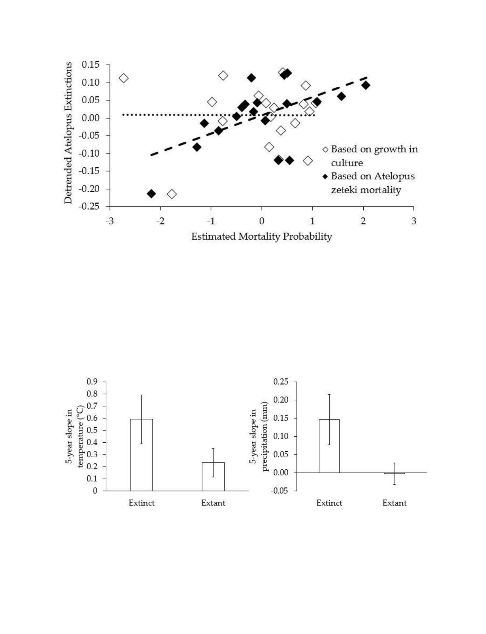
95
Figure 5.3. Predicting extinctions with results of temperature-dependent Bd growth
experiments. Using the linear equation derived from the temperature-dependent pattern of
Bdexposed A. zeteki mortality in the lab (Fig. 1), yearly temperature-based mortality probabilities
(presented as Z-scores) are a good predictor of detrended extinctions in the field (closed
diamonds, dashed line, R2=.303, p=.01). Meanwhile, the equation derived from the unimodal
temperature-dependent pattern of Bd growth in culture (Fig. 1) is a poor predictor of extinctions
(open diamonds, dotted line, R2<.001, p=.98).
Figure 5.4. Five-year slopes in climatic variables prior to Atelopus spp. extinctions. To
compare climate change between extinct and extant Atelopus spp., we matched each five-year
climate slope before extinction to the slope simultaneously experienced by all extant species.
Temperature increased ~2.5 times faster in the five years before extinction for extinct compared
to extant species (F1,45=7.73, p<.01; Fig. 4). In addition, the rate of increase in precipitation levels

96
was also higher among extinct species (F1,45=4.17, p<.05), likely because Bd can only survive in
moist conditions. Error bars represent standard errors.
References
Alford, R. A., K. S. Bradfield, et al. (2007). "Ecology - Global warming and amphibian losses."
Nature 447(7144): E3-E4.
Angilletta Jr, M. J. (2006). "Estimating and comparing thermal performance curves." Journal of
Thermal Biology 31(7): 541-545.
Bates, D., M. Maechler, et al. (2014). "lme4: Linear mixed-effects models using Eigen and S4, R
package version 1.1-6."
Bolker, B. (2014). "bbmle: Tools for general maximum likelihood estimation, R package version
1.0.16."
Boyle, D. G., D. B. Boyle, et al. (2004). "Rapid quantitative detection of chytridiomycosis
(Batrachochytrium dendrobatidis) in amphibian samples using real-time Taqman PCR
assay." Diseases of Aquatic Organisms 60(2): 141-148.
Cahill, A. E., M. E. Aiello-Lammens, et al. (2013). "How does climate change cause extinction?"
Proceedings of the Royal Society B-Biological Sciences 280(1750).
Cohen, J., M. Venesky, et al. (in prep). "The thermal mismatch hypothesis explains outbreaks of
an emerging infectious disease."
Collins, J. P. (2013). "History, novelty, and emergence of an infectious amphibian disease."
Proceedings of the National Academy of Sciences of the United States of America
110(23): 9193-9194.

97
Dell, A. I., S. Pawar, et al. (2011). "Systematic variation in the temperature dependence of
physiological and ecological traits." Proceedings of the National Academy of Sciences of
the United States of America 108(26): 10591-10596.
Ermert, V., A. H. Fink, et al. (2012). "The Impact of Regional Climate Change on Malaria Risk
due to Greenhouse Forcing and Land-Use Changes in Tropical Africa." Environmental
Health Perspectives 120(1): 77-84.
Harris, I., P. D. Jones, et al. (2014). "Updated high-resolution grids of monthly climatic
observations – the CRU TS3.10 Dataset." International Journal of Climatology 34(3):
623-642.
Harvell, C. D., C. E. Mitchell, et al. (2002). "Ecology - Climate warming and disease risks for
terrestrial and marine biota." Science 296(5576): 2158-2162.
Hijmans, R. J. (2014). "raster: Geographic data analysis and modeling, R package version
2.2.31."
Karraker, N. E., C. L. Richards, et al. (2006). "Reproductive Ecology of Atelopus zeteki and
Comparisons to other members of the genus." Herpetological review 37(3): 284-288.
Kilpatrick, A. M., C. J. Briggs, et al. (2010). "The ecology and impact of chytridiomycosis: an
emerging disease of amphibians." Trends in Ecology & Evolution 25(2): 109-118.
La Marca, E., K. R. Lips, et al. (2005). "Catastrophic population declines and extinctions in
neotropical harlequin frogs (Bufonidae : Atelopus)." Biotropica 37(2): 190-201.
Lafferty, K. D. (2009). "The ecology of climate change and infectious diseases." Ecology 90(4):
888-900.
Lips, K. R., J. Diffendorfer, et al. (2008). "Riding the wave: Reconciling the roles of disease and
climate change in amphibian declines." Plos Biology 6(3): 441-454.

98
Liu, X., J. R. Rohr, et al. (2013). "Climate, vegetation, introduced hosts and trade shape a global
wildlife pandemic." Proceedings of the Royal Society B-Biological Sciences 280(1753).
Maher, S. P., A. M. Kramer, et al. (2012). "Spread of white-nose syndrome on a network regulated
by geography and climate." Nature Communications 3.
Murray, K. A., R. W. R. Retallick, et al. (2011). "Assessing spatial patterns of disease risk to
biodiversity: implications for the management of the amphibian pathogen,
Batrachochytrium dendrobatidis." Journal of Applied Ecology 48(1): 163-173.
Pascual, M., L. F. Chaves, et al. (2008). "Predicting endemic cholera: the role of climate
variability and disease dynamics." Climate Research 36(2): 131-140.
Patz, J. A., D. Campbell-Lendrum, et al. (2005). "Impact of regional climate change on human
health." Nature 438(7066): 310-317.
Piotrowski, J. S., S. L. Annis, et al. (2004). "Physiology of Batrachochytrium dendrobatidis, a
chytrid pathogen of amphibians." Mycologia 96(1): 9-15.
Pounds, J. A., M. R. Bustamante, et al. (2006). "Widespread amphibian extinctions from epidemic
disease driven by global warming." Nature 439(7073): 161-167.
Raffel, T. R., N. T. Halstead, et al. (2015). "Temperature variability and moisture synergistically
interact to exacerbate an epizootic disease." Proceedings of the Royal Society B-
Biological Sciences 282(1801).
Raffel, T. R., J. M. Romansic, et al. (2013). "Disease and thermal acclimation in a more variable
and unpredictable climate." Nature Climate Change 3(2): 146-151.
Rodder, D., J. Kielgast, et al. (2010). "Future potential distribution of the emerging amphibian
chytrid fungus under anthropogenic climate change." Diseases of Aquatic Organisms
92(2-3): 201-U118.
Rohr, J. R., A. P. Dobson, et al. (2011). "Frontiers in climate change-disease research." Trends in

99
Ecology & Evolution 26(6): 270-277.
Rohr, J. R. and T. R. Raffel (2010). "Linking global climate and temperature variability to
widespread amphibian declines putatively caused by disease." Proceedings of the National
Academy of Sciences of the United States of America 107(18): 8269-8274.
Rohr, J. R., T. R. Raffel, et al. (2008). "Evaluating the links between climate, disease spread, and
amphibian declines." Proceedings of the National Academy of Sciences of the United
States of America 105(45): 17436-17441.
Skerratt, L. F., L. Berger, et al. (2007). "Spread of chytridiomycosis has caused the rapid global
decline and extinction of frogs." Ecohealth 4(2): 125-134.
Stenseth, N. C., A. Mysterud, et al. (2002). "Ecological effects of climate fluctuations." Science
297(5585): 1292-1296.
Team, R. C. (2014). R: A language and environment for statistical computing. R Foundation for
Statistical Computing, Vienna, Austria.
Therneau, T. (2014). "A Package for Survival Analysis in S, R package version 2.37.7."
Woodhams, D. C., R. A. Alford, et al. (2008). "Life-history trade-offs influence disease in
changing climates: Strategies of an amphibian pathogen." Ecology 89(6): 1627-1639.
CHAPTER SIX: CONCLUSION

100
Main Text
The ecological impacts of climate change are expected to include shifts to the phenology
(Root, Price et al. 2003; Ovaskainen, Skorokhodova et al. 2013; While and Uller 2014),
distributions (Walther, Post et al. 2002; Parmesan and Yohe 2003; Ostfeld and Brunner 2015), and
body sizes (Gardner, Peters et al. 2011) of organisms, alterations to species interactions and
disease outcomes (Lafferty 2009; Rohr and Raffel 2010; Raffel, Romansic et al. 2013), changes to
community composition (Walther, Post et al. 2002; Moritz, Patton et al. 2008), and loss of
available habitat (Thomas, Cameron et al. 2004; Mac Nally, Bennett et al. 2009). However,
directional predictions about these effects are often generalized, broad, and sweeping (Rohr,
Dobson et al. 2011; Altizer, Ostfeld et al. 2013). For example, debates over the impacts of climate
change-induced homogenization of biodiversity on disease outcomes generally focus on whether
the impact will be evident at all, rather than the sets of circumstances that are likely to promote or
impede it (Ostfeld and Keesing 2000; Randolph and Dobson 2012; Wood and Lafferty 2013).
Broadly, some debates over the effects of climate change on infectious disease have operated as if
the intensity of disease will always either remain stable or increase under all circumstances,
leaving little room for more nuanced outcomes (Lafferty 2009; Rohr, Dobson et al. 2011; Altizer,
Ostfeld et al. 2013). Often, a specific set of climatic conditions are assumed to promote infectious
disease outbreaks for a given disease, while possible taxonomic-level differences in conditions
are ignored. Similarly, studies often draw conclusions about the climatic factors associated with
phenological advancement globally, based only on one or a handful of case studies within a small
area (Rubolini, Moller et al. 2007; Thackeray, Henrys et al. 2016). Finally, while distributional
range shifts and changes to body size are commonly expected to be universal responses to
warming, there is significant heterogeneity in the direction and magnitude of these responses and
data is lacking for a number of taxa (Chen, Hill et al. 2011; Li, Cohen et al. 2013).

101
In truth, influences of climate change on organisms and ecosystems are likely to be more
nuanced. Temperature increases, changes to precipitation patterns, increases in temperature
variability and the frequency of extreme weather events are occurring heterogeneously in space,
not uniformly (Easterling, Meehl et al. 2000; Yeh, Kug et al. 2009; Cai, Borlace et al. 2014). Such
heterogeneous patterns in climate projections are already well accounted for in predictive models
of disease spread or dispersal shifts associated with climate change (Chen, Hill et al. 2011; Liu,
Rohr et al. 2013). However, models often fail to account for the fact that different organisms
existing in the same location are often experiencing their environments on different spatial and
temporal scales, and thus, may only be subject to processes that occur at those scales. For
example, small organisms, which generally occupy smaller ranges and have faster pace of life
than larger organisms (Promislow and Harvey 1990; Speakman 2005), could be more vulnerable
to shifting ecological processes that take place at small spatial scales (e.g., microclimates) and
shorter temporal scales. Meanwhile, larger, slower-paced organisms could be impacted by
processes taking place at large, regional spatial scales and long temporal scales. Thus, theory is
needed to account for the ways in which large variation in spatial and temporal scales influences
the importance of various biotic and abiotic factors in determining ecological patterns (although
we have recent tests across relatively narrow scale ranges, see (Chase and Leibold 2002; Rahbek
2005)). I hypothesized in my dissertation that many of the processes controlling the ecological
impacts of climate change are likely to predictable depending on the relevant spatial or temporal
scale. Indeed, based on my results, I conclude that climate change will have diverse and
sometimes opposing effects on organisms across spatial, temporal and allometric scales.

102
Climate change across spatial scales
In my first chapter, I set out to test a longstanding hypothesis about the influence of spatial
scale on ecological patterns that, if confirmed, could inform predictions about how climate
change will impact ecosystems. I examined whether factors controlling the distributions of three
diseases across spatial scales – amphibian chytridiomycosis (caused by the fungal pathogen
Batrachochytrium dendrobatidis, or Bd), West Nile virus, and Lyme disease – could be predicted
based on a fundamental hypothesis in ecology: that biotic processes control ecological patterns,
such as species distributions, at small, local scales while abiotic processes do so at large, regional
scales (Wiens 1989; Levin 1992). This decades-old hypothesis was poorly tested because the
necessary species distribution datasets and computing power were not historically available.
Indeed, I found that a biotic process representing biodiversity, species richness, was highly
predictive of all three diseases at local scales, while temperature, precipitation and other abiotic
factors predicted disease distributions at regional scales. Critically, I found that there was no
single spatial scale where both biotic and abiotic processes were predictive of the distribution of
any disease.
This work has important implications for understanding how climate change will alter the
distribution of species. At large scales, species’ ranges are likely to be directly impacted by
climate change via changes to broad-scale temperature and precipitation patterns. At small scales,
climate change may have more indirect impacts on species; for example, alterations to
community composition could impact the level of disease that an organism is exposed to via the
dilution effect. Climate change is altering weather patterns, community composition, and species
dispersal and distribution across spatial scales; therefore, it is critical for researchers to be able to
predict which factors will influence the dispersal of organisms, including those that are invasive

103
pests or cause disease outbreaks. An important upshot to my results, which appear to confirm this
longstanding hypothesis, is that the importance of some ecological processes that dictate the
distribution of species can be highly underestimated when the appropriate scale is not considered.
For example, controversy over the existence of the dilution effect, or the hypothesized
negative relationship between species richness and disease prevalence, may at least partially be a
result of the scale at which studies have been conducted (Civitello, Cohen et al. 2015; Johnson,
Ostfeld et al. 2015). Previous tests of the dilution effect at large, regional spatial scales found that
it was relatively small compared to the effects of climate, even though it was strongly detected in
laboratory experiments (Venesky, Liu et al. 2014). A separate analysis of the biotic, abiotic, and
propagule pressure factors controlling Bd distribution also found no importance of biotic factors
at regional scales (Liu, Rohr et al. 2013). In contrast, several studies conducted at relatively small
scales have found significant effects of dilution (LoGiudice, Ostfeld et al. 2003; Ezenwa, Godsey
et al. 2006; Werden, Barker et al. 2014). In my findings, host species richness was only predictive
of the distribution of Bd, Lyme disease and West Nile virus at the smallest spatial scales tested. If
biotic factors such as species interactions or biodiversity primarily control disease distributions at
small, local scales, the dilution effect might only be detectable at these scales, possibly explaining
part of the controversy.
An improved consideration of spatial scale can also provide insights into factors controlling
phenological shifts. Syntheses tracking several species in one or several localized areas have
concluded that changes in temperature alone are responsible for driving phenological shifts
(Menzel, Sparks et al. 2006; Gienapp, Leimu et al. 2007). However, the results of my broad scale,
global meta-analysis indicate that there are regional differences in the climate factors driving
shifts. For example, while temperature strongly drives phenological shifts at high latitudes,

104
precipitation is an important driver at lower latitudes. On the other hand, my results suggest that
local-scale data should be used to examine the importance of ecological communities on
influencing asynchrony in species interactions (e.g., mismatches between flowers and
pollinators), an important side effect of phenological shifts.
Finally, consideration of scale could be useful in understanding widespread extinctions driven
by an interaction between climate change and emerging disease. Previous studies that examined
localized outbreaks of Bd in Atelopus spp. found a multidecadal, genus-wide positive relationship
between outbreaks and mean temperature despite using continental or global-scale climate data
(Pounds, Bustamante et al. 2006; Rohr and Raffel 2010). Analyses at this spatial scale may have
been inappropriate because conditions in the mostly small, isolated, mountaintop ranges of
Atelopus spp. may be very different from those over the mostly lowland continent or tropical
global biome. My analysis using finer-scale regional data restricted to the individual species
ranges in Atelopus suggested that rapid increases in temperature over the course of only several
years in combination with disease spread were driving individual species extinct, adding an
important dimension to the interpretation of these climate-driven extinctions. Using only
broadscale climate data, it would have been impossible to tease apart what was going on in
individual species ranges prior to each extinction.
Climate change across temporal and allometric scales
Climate change is causing global mean temperatures to shift at an unprecedented rate and is
increasing temperature variability, or the frequency of temperature shifts (Easterling, Meehl et al.

105
2000; Pachauri, Allen et al. 2014). Thus, climate change is changing the conditions that organisms
experience across moderate (multi-decadal) and short (daily to annual) temporal scales. Small
organisms should be more adaptable to longer-term, multi-decadal changes in climate given their
shorter generation times (Speakman 2005). Therefore, I hypothesized that small organisms would
track longer-term temperature shifts by shifting their phenology more rapidly than larger
organisms. Indeed, in my second chapter I found a significant negative relationship between body
size and phenological shifts, suggesting that small organisms are shifting their phenology with
climate change much faster than large organisms. This has several implications for species
interactions in future ecological communities. For example, prey are typically smaller than their
predators, and if they shift their phenology earlier, predators may miss key windows where prey
are abundant following migration or breeding (Visser, Both et al. 2004). Similarly, because
parasites are often orders of magnitude smaller than their hosts, climate change could result in
asynchrony in host-parasite interactions (Mas-Coma, Valero et al. 2009). Thus, changes to climate
over long temporal scales could disrupt a variety of important species interactions.
In addition, smaller organisms, such as parasites, should be better equipped to handle
shortterm temperature variability because they acclimate to new conditions faster than larger
organisms (Baas-Becking 1934; Raffel, Romansic et al. 2013; Rohr, Civitello et al. in review),
such as hosts, likely owing to their faster metabolic rates (Gillooly, Brown et al. 2001; Brown,
Gillooly et al. 2004). Thus, under variable conditions, smaller organisms should have functionally
larger thermal performance breadths, or temperature ranges where performance is relatively strong
(Rohr, Civitello et al. in review). I predicted that gaps between host and parasite performance would
appear at relatively cold and warm temperatures for warm- and cold-adapted hosts, respectively,
because hosts and parasites are likely to be locally adapted to the conditions in their environments
and parasites are likely to be limited by extreme conditions despite their broad breadths.

106
In my third chapter, I tested whether warm- and cold-adapted amphibian species were likely
to experience susceptibility to Bd under differing conditions using a series of
temperaturedependent Bd growth experiments and a dataset containing 4,775 record of
populations tested for Bd in the field. My results illustrated that in both the lab and the field,
warm-adapted amphibians were more likely to have high Bd prevalence and intensity under cool
conditions (~10-16 C), while cold-adapted species were likely to experience outbreaks under
relatively warm conditions (~21-26 C). Thus, cold-adapted hosts may soon be at greater risk of
disease because they are likely to have performance gaps with parasites under warming
conditions. Similarly, recent simulation models have suggested that large-bodied, low-latitude
amphibian species are more likely than other amphibians to experience lethal and sub-lethal
effects with increasing climate change, likely because of their longer acclimation times and
relative disadvantage with parasites (Rohr, Civitello et al. in review). Finally, while these results
only speak to changing host-parasite dynamics across multi-decadal time scales, recent work
suggests that increasing temperature variability should lend parasites at advantage under
weeklong time scales (Raffel, Romansic et al.
2013), because parasites should acclimate to temperature shifts faster than hosts.
Based on my dissertation results, I conclude that small organisms may be better equipped to
handle changing climatic conditions across short to multi-decadal temporal scales. Although I
could not test species’ responses to climate change over longer scales, some evidence suggests
that small organisms possess an adaptive advantage at century-long scales as well (Genner, Sims
et al. 2010). However, there are some circumstances under which larger organisms may cope well
with climate change. First, large organisms have larger range sizes (Lindstedt, Miller et al. 1986)
and may therefore be less susceptible to small-scale habitat loss induced by climate change, such
as loss of coastal habitat. Unfortunately, if large organisms have large range requirements, they

107
may be at a disadvantage following broad-scale habitat loss, such as climate change-induced
desertification. Second, because large organisms are better dispersers (Gaston 2003;
BohningGaese, Caprano et al. 2006), they may do a better job of shifting their ranges to counter
changing conditions (Kaustuv, Jablonski et al. 2001). Despite this, some evidence indicates that
smaller fish are shifting their ranges northward at a greater rate than larger fish (Perry, Low et al.
2005). Finally, recent evidence suggests that organisms are evolving smaller body sizes as an
additional method to cope with climate change (Gardner, Peters et al. 2011; Sheridan and
Bickford 2011), because decreasing surface-area to mass ratios allow organisms to increase
evaporative heat loss.
Conclusion
Anthropogenic change, including climate change, is occurring across a wide range of spatial
and temporal scales. My dissertation chapters tackled diverse hypotheses concerning how spatial
and temporal scales will modulate the impacts of climate change. My first chapter confirmed a
longstanding hypothesis in ecology: that biotic factors influence ecological patterns at local
spatial scales, while abiotic factors control patterns at regional scales (Wiens 1989; Levin 1992).
My later chapters applied this lesson by examining how the climatic factors associated with
phenological shifts and disease outbreaks may depend on the spatial scale at which data is
analyzed. Finally, throughout my dissertation, small organisms maintained advantages over larger
organisms across temporal scales, likely because they are due in part to their ability to better cope
with changing temperature conditions (Rohr, Civitello et al. in review). Importantly, these
conclusions suggest that parasites may gain crucial advantages over their typically larger hosts
with increasing long-term temperature means and greater short-term temperature variability. In

108
summary, my research has contributed to what we understand about scale, disease, and
biodiversity declines in the context of climate change.

109
References
Altizer, S., R. S. Ostfeld, et al. (2013). "Climate Change and Infectious Diseases: From Evidence
to a Predictive Framework." Science 341(6145): 514-519.
Baas-Becking, L. G. M. (1934). Geobiologie; of inleiding tot de milieukunde, WP Van Stockum
& Zoon NV.
Bohning-Gaese, K., T. Caprano, et al. (2006). "Range size: Disentangling current traits and
phylogenetic and biogeographic factors." American Naturalist 167(4): 555-567.
Brown, J. H., J. F. Gillooly, et al. (2004). "Toward a metabolic theory of ecology." Ecology
85(7): 1771-1789.
Cai, W. J., S. Borlace, et al. (2014). "Increasing frequency of extreme El Nino events due to
greenhouse warming." Nature Climate Change 4(2): 111-116.
Chase, J. M. and M. A. Leibold (2002). "Spatial scale dictates the productivity-biodiversity
relationship." Nature 416(6879): 427-430.
Chen, I. C., J. K. Hill, et al. (2011). "Rapid Range Shifts of Species Associated with High Levels
of Climate Warming." Science 333(6045): 1024-1026.
Civitello, D. J., J. Cohen, et al. (2015). "Biodiversity inhibits parasites: Broad evidence for the
dilution effect." Proceedings of the National Academy of Sciences of the United States of
America 112(28): 8667-8671.
Easterling, D. R., G. A. Meehl, et al. (2000). "Climate extremes: Observations, modeling, and
impacts." Science 289(5487): 2068-2074.
Ezenwa, V. O., M. S. Godsey, et al. (2006). "Avian diversity and West Nile virus: testing
associations between biodiversity and infectious disease risk." Proceedings of the Royal
Society B-Biological Sciences 273(1582): 109-117.

110
Gardner, J. L., A. Peters, et al. (2011). "Declining body size: a third universal response to
warming?" Trends in Ecology & Evolution 26(6): 285-291.
Gaston, K. J. (2003). "Ecology - The how and why of biodiversity." Nature 421(6926): 900-901.
Genner, M. J., D. W. Sims, et al. (2010). "Body size‐dependent responses of a marine fish
assemblage to climate change and fishing over a century‐long scale." Global Change
Biology 16(2): 517-527.
Gienapp, P., R. Leimu, et al. (2007). "Responses to climate change in avian migration time -
microevolution versus phenotypic plasticity." Climate Research 35(1-2): 25-35.
Gillooly, J. F., J. H. Brown, et al. (2001). "Effects of size and temperature on metabolic rate."
Science 293(5538): 2248-2251.
Johnson, P. T. J., R. S. Ostfeld, et al. (2015). "Frontiers in research on biodiversity and disease."
Ecology Letters 18(10): 1119-1133.
Kaustuv, R., D. Jablonski, et al. (2001). "Climate change, species range limits and body size in
marine bivalves." Ecology Letters 4(4): 366-370.
Lafferty, K. D. (2009). "The ecology of climate change and infectious diseases." Ecology 90(4):
888-900.
Levin, S. A. (1992). "The Problem of Pattern and Scale in Ecology." Ecology 73(6): 1943-1967.
Li, Y. M., J. M. Cohen, et al. (2013). "Review and synthesis of the effects of climate change on
amphibians." Integrative Zoology 8(2): 145-161.
Lindstedt, S. L., B. J. Miller, et al. (1986). "Home Range, Time, and Body Size in Mammals."
Ecology 67(2): 413-418.
Liu, X., J. R. Rohr, et al. (2013). "Climate, vegetation, introduced hosts and trade shape a global
wildlife pandemic." Proceedings of the Royal Society B-Biological Sciences 280(1753).

111
LoGiudice, K., R. S. Ostfeld, et al. (2003). "The ecology of infectious disease: Effects of host
diversity and community composition on Lyme disease risk." Proceedings of the National
Academy of Sciences of the United States of America 100(2): 567-571.
Mac Nally, R., A. F. Bennett, et al. (2009). "Collapse of an avifauna: climate change appears to
exacerbate habitat loss and degradation." Diversity and Distributions 15(4): 720-730.
Mas-Coma, S., M. A. Valero, et al. (2009). "Climate change effects on trematodiases, with
emphasis on zoonotic fascioliasis and schistosomiasis." Veterinary Parasitology 163(4):
264-280.
Menzel, A., T. H. Sparks, et al. (2006). "European phenological response to climate change
matches the warming pattern." Global Change Biology 12(10): 1969-1976.
Moritz, C., J. L. Patton, et al. (2008). "Impact of a century of climate change on small-mammal
communities in Yosemite National Park, USA." Science 322(5899): 261-264.
Ostfeld, R. S. and J. L. Brunner (2015). "Climate change and Ixodes tick-borne diseases of
humans." Philosophical Transactions of the Royal Society B-Biological Sciences
370(1665).
Ostfeld, R. S. and F. Keesing (2000). "Biodiversity and disease risk: The case of lyme disease."
Conservation Biology 14(3): 722-728.
Ovaskainen, O., S. Skorokhodova, et al. (2013). "Community-level phenological response to
climate change." Proceedings of the National Academy of Sciences of the United States of
America 110(33): 13434-13439.
Pachauri, R. K., M. R. Allen, et al. (2014). Climate change 2014: synthesis Report. Contribution
of working groups I, II and III to the fifth assessment report of the intergovernmental
panel on climate change, IPCC.

112
Parmesan, C. and G. Yohe (2003). "A globally coherent fingerprint of climate change impacts
across natural systems." Nature 421(6918): 37-42.
Perry, A. L., P. J. Low, et al. (2005). "Climate change and distribution shifts in marine fishes."
Science 308(5730): 1912-1915.
Pounds, J. A., M. R. Bustamante, et al. (2006). "Widespread amphibian extinctions from epidemic
disease driven by global warming." Nature 439(7073): 161-167.
Promislow, D. E. L. and P. H. Harvey (1990). "Living Fast and Dying Young - a Comparative-
Analysis of Life-History Variation among Mammals." Journal of Zoology 220: 417-437.
Raffel, T. R., J. M. Romansic, et al. (2013). "Disease and thermal acclimation in a more variable
and unpredictable climate." Nature Climate Change 3(2): 146-151.
Rahbek, C. (2005). "The role of spatial scale and the perception of large-scale species-richness
patterns." Ecology Letters 8(2): 224-239.
Randolph, S. E. and A. D. M. Dobson (2012). "Pangloss revisited: a critique of the dilution effect
and the biodiversity-buffers-disease paradigm." Parasitology 139(7): 847-863.
Rohr, J., D. J. Civitello, et al. (in review). "A global framework for estimating acclimation and
thermal breadth predicts risk from climate change " Proceedings of the National Academy
of Sciences of the United States of America.
Rohr, J. R., A. P. Dobson, et al. (2011). "Frontiers in climate change-disease research." Trends in
Ecology & Evolution 26(6): 270-277.
Rohr, J. R. and T. R. Raffel (2010). "Linking global climate and temperature variability to
widespread amphibian declines putatively caused by disease." Proceedings of the National
Academy of Sciences of the United States of America 107(18): 8269-8274.
Root, T. L., J. T. Price, et al. (2003). "Fingerprints of global warming on wild animals and plants."
Nature 421(6918): 57-60.

113
Rubolini, D., A. P. Moller, et al. (2007). "Intraspecific consistency and geographic variability in
temporal trends of spring migration phenology among European bird species." Climate
Research 35(1-2): 135-146.
Sheridan, J. A. and D. Bickford (2011). "Shrinking body size as an ecological response to climate
change." Nature Climate Change 1(8): 401-406.
Speakman, J. R. (2005). "Body size, energy metabolism and lifespan." Journal of Experimental
Biology 208(9): 1717-1730.
Thackeray, S. J., P. A. Henrys, et al. (2016). "Phenological sensitivity to climate across taxa and
trophic levels." Nature.
Thomas, C. D., A. Cameron, et al. (2004). "Extinction risk from climate change." Nature
427(6970): 145-148.
Venesky, M. D., X. Liu, et al. (2014). "Linking manipulative experiments to field data to test the
dilution effect." Journal of Animal Ecology 83(3): 557-565.
Visser, M. E., C. Both, et al. (2004). "Global climate change leads to mistimed avian
reproduction." Birds and Climate Change 35: 89-110.
Walther, G. R., E. Post, et al. (2002). "Ecological responses to recent climate change." Nature
416(6879): 389-395.
Werden, L., I. K. Barker, et al. (2014). "Geography, Deer, and Host Biodiversity Shape the Pattern
of Lyme Disease Emergence in the Thousand Islands Archipelago of Ontario,
Canada." PLoS ONE 9(1).
While, G. M. and T. Uller (2014). "Quo vadis amphibia? Global warming and breeding
phenology in frogs, toads and salamanders." Ecography 37(10): 921-929.
Wiens, J. A. (1989). "Spatial Scaling in Ecology." Functional Ecology 3(4): 385-397.

114
Wood, C. L. and K. D. Lafferty (2013). "Biodiversity and disease: a synthesis of ecological
perspectives on Lyme disease transmission." Trends in Ecology & Evolution 28(4):
239247.
Yeh, S. W., J. S. Kug, et al. (2009). "El Nino in a changing climate." Nature 461(7263): 511-
U570.

115
APPENDICES

116
Appendix A: Supplementary Materials: Chapter Two
Supplementary Discussion
Human-assisted dispersal
Humans may have a variety of effects on the distribution of organisms including effects on their
dispersal. Dispersal is an important factor controlling species distributions even when those
distributions appear stable because species are always in dynamic disequilibrium (Heaney 2000).
For example, continuous disturbances to the landscape, community composition, or microclimate
caused by humans can result in perpetual mismatches between a species’ current and potential
distribution (Sexton, McIntyre et al. 2009). Therefore, we tested whether human population
density affected the distributions of Bd, WNV and Lyme disease despite controversy surrounding
whether their ranges are expanding or are stable.
Heterogeneity of residuals in space
In the Bd models, at scales in which predictors in our models influenced the residuals, residuals
were mostly altered homogenously in space (Figure 3). However, spatial heterogeneity among
residuals was observed in the WNV and Lyme models (Figure A2). Very high or low residuals
may be observed at the highest or lowest latitudes on abiotic maps because predictors may act
most strongly where they are most limiting to disease ranges. Alternatively, the residuals may be
high in these areas because the underlying predictor values are more extreme. For example,
Florida often has high residuals on the abiotic maps because it has very high temperatures. In
addition, clustering of similar residuals may be especially profound in human population density
maps because of extreme human density values. Finally, in Wisconsin, which has a very high

117
incidence of Lyme disease, our models generally did a poor job at predicting the incidence of this
disease.
Consideration of vectors
The need to consider the conditions favoring the vector is important when attempting to
understand the distribution of a vector-borne pathogen. We considered adding information about
the vectors as predictors into our primary statistical analyses of West Nile virus and Lyme disease
but chose not to do so for several reasons. First, our analyses implicitly already consider vectors
because our response data are human disease cases. Humans cannot be infected unless they are
bitten by the appropriate vector and thus the distribution of the pathogen in humans importantly
integrates the effects of abiotic, biotic, and propagule pressure factors on the pathogen,
intermediate hosts, and the vectors. Therefore, the conditions that can support disease already
reflect those that can support the pathogen, vector and host, and it should not be necessary to
examine the vector independently.
Nevertheless, we did consider the possibility that accounting for the vector distribution
could reduce the amount of error variance and thus increase our statistical power to detect the
effects of interest. We obtained geographic distribution maps for the vectors of West Nile virus
(Culex sp. and other mosquito species) (Ciota and Kramer 2013) and Lyme disease (Ixodes
scapularis) (CDC), but these maps revealed that these vectors are spread throughout the entire
spatial extent of our statistical analyses (Eastern U.S., east of the Mississippi river). Thus, we
could not use presence/absence of the vector as a predictor in our models because there was no
variation in presence/absence among the counties in the eastern U.S. based on the range maps for
the primary vectors. However, we collected presence/absence maps of individual mosquito

118
species (VectorMaps) and generated vector richness rasters for the Eastern U.S., including these
in preliminary West Nile virus models, although this predictor was not significant at any scale.
Additionally, we included abundance of waterbodies in our model for West Nile virus because
mosquitoes require water to breed and it did not change our results either.
Importantly, many studies do not include every possible variable that affects disease.
However, we do acknowledge that the lack of inclusion a predictor can present a “third variable”
problem. That is, a researcher could conclude that a relationship is causal when in fact the
correlated third variable that was not included is the real causal factor. However, we are not
suggesting that each of the variables we tested is the cause of a change in the focal disease.
Rather, we are suggesting that biotic factors in general (whether they are truly causal or not) are
more predictive on small scales and abiotic factors (whether they are truly causal or not) are more
predictive at larger scales. The fact that we implicitly rather than explicitly consider vectors
should in no way invalidate this general conclusion. For all the reasons above, we decided
against explicitly incorporating vector presence, abundance, or suitability into our models but, to
reiterate, the vector is still indirectly or implicitly included as component of our models.
Consideration of interactions between predictors
There are several reasons why we chose not to test for interactions, some of which were explained
in the manuscript and the other explanations have been added. 1) Interactions cannot be classified
as “biotic predictors”, “abiotic predictors”, or “human population effects” because they would
always have predictors from at least two of these categories. Hence, because they are impossible
to categorize according to the focal hypothesis of our paper, they prevent us from addressing the
main goal of the paper, which is to test whether biotic and abiotic predictors are relatively
important at the same or differing spatial scales. 2) We lack any a priori hypotheses regarding the

119
spatial scales where interactions may be relevant, or even which interactions may be important.
3) To conduct a single analysis on one parasite across all seven scales controlling for spatial auto-
correlation with multimodel inference and limiting the model to only three predictors or less takes
approximately one week. Adding in interactions exponentially increases the number of models,
would require us to consider models with more than three predictors (because a single two-way
interaction alone requires three variables because the two main effects must be included), and
thus quickly makes the analyses intractable. With 5 predictors, there would be 32 possible
interactions per model, resulting in hundreds of millions of possible models for MuMIn to
evaluate per parasite per scale. Even on a super computer, this would currently be an intractable
problem to address. 4) Finally, this exercise is not about coming up with a model that maximizes
our ability to predict prevalence. That would require considering interactions and other candidate
variables. The goal is to assess whether the importance of classes of predictors varies across
spatial scales in a consistent and predictable manner across different types of hostparasite
systems. This, however, is not to downplay the importance of interaction or improving the fit of
statistical models. Indeed, interactions might be very important and might also depend on scale.
But, they are not crucial to our hypotheses and, just like computing limitations at least partially
prevented researchers from testing many scales hypotheses before now, computing limitations are
still making it challenging to thoroughly consider interactions across scales when spatial
autocorrelation and multimodel inference approaches are used.

120
Assessing model predictability
We computed the root mean square error (RMSE) for the model-averaged predictions for each
parasite at each scale (Table A5). The RMSE is a well-established criterion for evaluating
predictive capability and it has several advantages for our analysis. First, it allows us to compare
the predictive performance for each parasite across each scale. Second, it retains a valid
interpretation for models that incorporate spatial autocorrelation, unlike R2 or pseudo-R2 values.
Third, it can be computed from our completed analysis, rather than via resampling analyses,
which we found would take months. Lastly, it has a simple interpretation: it represents the mean
deviation between the observed and predicted values, so smaller values indicate better overall
performance. Analyses based on RMSE can indicate whether our predictions changed in accuracy
across scales, contributing to what we understand about working with data across spatial scale in
ecology.
Supplementary Methods
Conversion of species range polygons to richness rasters
We could not convert polygons directly to rasters while calculating the number of unique host
species per cell because the rasterize function only counts a polygon as being present in a cell if it
passes through the center of the cell, as opposed to overlapping any part of the cell. In many
studies this may not be an issue, but it would have prevented us from obtaining equally reliable
richness estimates across scales because host geographic ranges are less likely to cross the center
of a cell when the cells are larger. To work around this problem, we converted the geographic
range of each individual host species to a raster (All analyses were conducted in R 3.1.0 (2014);
raster package (Hijmans 2014), rasterize function) and then converted the rasters to spatial points

121
(rasterToPoints function). Points for all species within a taxon (i.e., amphibians) were then
combined into one dataset and combined with a blank raster template to create one raster
(rasterize function) at each of our scales. This process was repeated for each taxon. For unknown
reasons, some small, relatively isolated areas had extremely low polygon coverage (such as Long
Island for bird polygons) and so richness values in these areas were adjusted to the general
minimum in areas with proper coverage.
Pathogen-specific abiotic predictors.
In addition to the eight general abiotic variables summarized into factors, we also tested whether
water as a fraction of land cover predicted Bd and WNV prevalence, hypothesizing that water
cover may promote Bd and mosquito abundance. We downloaded 2011 edition land cover rasters
from the National Land Cover Database (http://www.mrlc.gov/nlcd2011.php) and masked them to
the U.S. or eastern U.S. for Bd and WNV, respectively (raster package (Hijmans 2014), mask
function). We categorized raster values as either land or freshwater and then aggregated the
values into cell sizes based on our seven scales (aggregate function) as outlined in the general
methods. Percent of wetland cover was used as a predictor in trial models alongside the three
other abiotic factors, richness, and human population density. Because this variable was not a
significant positive predictor of WNV or Bd distribution at any scale, we did not include it in any
reported models.
Vector Richness
We collected range maps for individual mosquito species from VectorMaps
(http://www.vectormap.org/Mosquito_Metadata.htm) as rasters. Rasters were adjusted to have a
common projection (projectRaster function, raster package (Hijmans 2014)) and spatial extent

122
(extent function) and were overlaid (summed) to generate counts of species across space. Rasters
were then upscaled and standardized in a similar manner as in the generation of other richness
rasters. We included mosquito richness rasters in preliminary multivariate GLS and MuMIn
models along with our other predictors and found that they were never significant at any scale
(Table A3), so we did not include this predictor in the models reported in the main text.
Other diseases or pathogens
We attempted to find spatially-explicit occurrence data for other widespread diseases including
rabies and avian malaria. While rabies data is collected and maintained by the Center for Disease
Control, it is not freely provided and can only be obtained by contacting each individual state.
Unfortunately, only a few states agreed to provide us with these data, preventing us from
obtaining a spatial extent large enough to test our hypotheses across a scale gradient. MalAvi
(http://mbio-serv2.mbioekol.lu.se/Malavi/), the largest database of avian malaria occurrence in
the world, has a few dozen records in the US at only a handful of locations, so we could not
examine the distribution of this disease either. We found no other spatially explicit disease
databases of sufficient extent to test our hypotheses.
Correlations between predictors
We tested for bivariate correlations among the predictors using the cor function in the stats
package of R statistical software.

123
Supplementary Results
Randomization tests
When the response data were randomized, none of the predictors were significant at any scale,
and all importance scores were small and equivalent across scales (Figure A3). Thus, our results
are not driven by unknown statistical artifacts, but rather appear to be a function of variation in
spatially-dependent ecological processes that dictate species distributions.
Univariate models
Effects of human population and richness were consistent with the results of multivariate models.
For all three diseases, the magnitude of coefficient for richness peaked at the smallest scale and
the coefficient for human population peaked at the largest scale (Figure A4). This suggests that
richness and human population were important at these scales in the multi-model inferences
because they became better predictors on their own. The abiotic factor coefficients were mostly
consistent across scales (although they peaked at large scales for Lyme disease; Figure A4),
suggesting that their high relative importances at moderate to larger scales may have been a result
of the changing significance of the other predictors.
Spatial correlograms
Whereas the univariate models provide a statistical mechanism for our results, the spatial
correlograms provide an ecological mechanism for our results. Traditionally, researchers
hypothesized that variables should be important at the scales where they vary the most. That is,
biotic factors should be important at small scales and abiotic factors should be important at larger

124
scales because each of these factors are thought to be more variable at these scales. To test this
hypothesis, we focused on WNV and Lyme because we had prevalence data evenly distributed
across the entire extent of the eastern U.S. (i.e. for every county), whereas for Bd, the data were
highly clumped making it challenging to obtain reliable estimates of autocorrelation.
Autocorrelation among host richness predictors for both WNV and Lyme decreased quickly,
reaching zero within approximately one degree (Figure A5). In contrast, factor one (representing
mostly temperature), the abiotic factor consistently relevant in our relative importance results,
remained autocorrelated for two to four degrees (Figure A5). Hence, as predicted, the
correlograms demonstrate that richness was more variable (low autocorrelation) than climate at
small scales and abiotic factors only became variable (high autocorrelation) at larger scales. This
is consistent with the hypothesis that variables should be relatively important at the scales that
they vary the most.
Predictions for scale-dependent dispersal limitations have always been less certain than
scale-dependent predictions for biotic and abiotic factors; moreover, our proxy for dispersal
limitations, human population density, does not capture dispersal only, making the findings for
human population density more difficult to interpret. Nevertheless, human population density
became uncorrelated within a half degree of distance (Figure A5).
Correlations between predictors
Predictors were not highly correlated to one another at any scale, although for some diseases there
was moderate correlation between richness and some abiotic factors (Table A4). However, this is
expected given that richness decreases from tropical to temperate zones. O’Brien et al.

125
(O'Brien 2007) and several other authors emphasize that the rule of thumb for multicollinearity
between two variables is an r2 ≥ 0.9 (or r ≥ 0.949), and even then, they discourage researchers
from eliminating or consolidating variables. The precision of parameter estimates is extremely
robust to correlations less than 0.9. Our highest correlation coefficients were nowhere near these
thresholds. Finally, our approach of model-averaged parameter estimation has been shown to
reduce the variance inflating effects of collinearity among predictors, especially in cases when all
predictors do not have strong effects simultaneously or correlations are not extreme.
Assessment of model error
We found that RMSE did not vary substantially across scales for any disease (Table A5),
suggesting that changing the scale of our analysis did not affect overall predictive power, but only
which predictors were influential. Additionally, the raw and standardized RMSE values in Table
A5 are quite small for both B. burgdorferi and West Nile virus (<0.038 for standardized RMSE),
the two parasites where we had the greatest amount and coverage of data (data for every county
across the US). Hence, the deviations between the predicted and observed values were small for
these models indicating that the models were good fits to the data. Not surprisingly, the RMSE
values for Bd are higher, presumably because of less data and worse spatial coverage for Bd than
for B. burgdorferi and West Nile virus. However, even the RMSE values for Bd are relatively
small (<0.271 for standardized RMSE), indicating that the deviations between the predicted and
observed values were not very substantial and that the model was a reasonable fit to the data. We
emphasize that we are receiving relatively good fits despite intentionally 1) not testing for
interactions that could improve model fits (see above for justification), and 2) not exhaustively
considering predictor variables.

126
Model averaging
The lists of models incorporated into each averaged model, along with their respective weights,
are presented in Table A6. In addition, we have presented model averaged outputs without
shrinkage in Table A7. However, we caution that parameter estimates with shrinkage are most
appropriate. In multiple regression analyses, estimates with shrinkage are preferable because they
reduce model selection bias (34, 35). By definition, shrinkage acknowledges that when a
predictor is not present in a model, this implies that its coefficient is zero. By including these
zeros in the model-averaging process, shrinkage reduces the upward bias that can be caused by
using only a single (or few) top model(s), and it drastically reduces the chance of Type-I error.
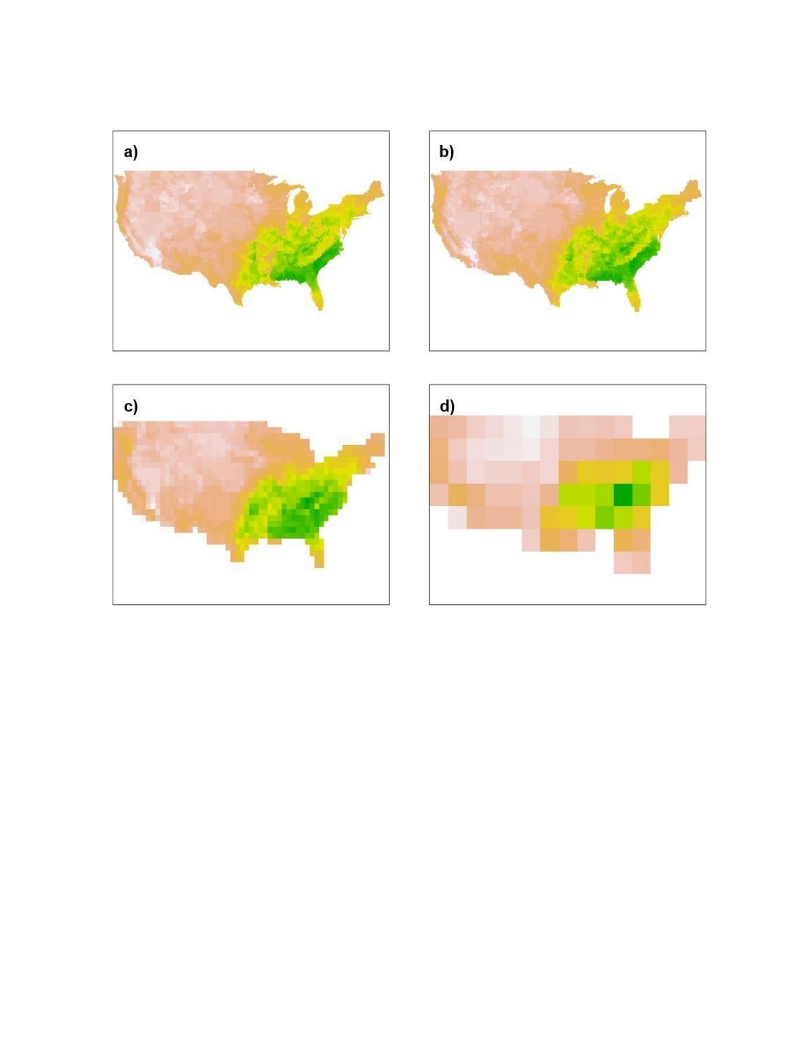
127
Supplementary Figures
Figure A1. Rasters of varying grain sizes were used in models. Sample rasters of amphibian
richness across scales with the following grain (cell) sizes: (a) 1/16th x 1/16th of a degree, (b) ¼ x
¼ of a degree, (c) 1 x 1 degree, (d) 4 x 4 degrees. Green cells represent high richness, yellow is
moderately high richness, orange is moderately low richness, and white is low. Amphibian
richness was used as a predictor in our Bd models. Rasters were scaled up by taking the mean of
the values in 2x2 grids of cells.

Biotic
Abiotic
Human
Effects
Spatial
scale
37
km?
600
km?
~10*
km?
~105
km?
128

129
Figure A2. Generality of scale-dependent processes in space. (Continued on next page)
Figure A2. Generality of scale-dependent processes in space. As in Figure 3, maps depict the
contribution of processes at varying spatial scales to models predicting county-level (a) Borrelia
burgdorferi and (b) West Nile virus data. The counties are colored based on the change in their
residuals after the given process was added to a model predicting parasite distribution. Blue
counties decreased the magnitude of the residuals (helped the model), red counties increased
them (hurt the model), while white counties did not affect the model. The color strength indicates
the magnitude of the change in residual. Maps with many colored counties represent scales at
which a given process was highly important, while maps with mostly white counties signify that a
process was not relevant at a given scale.

130
Figure A3. Null-model randomizations. Results of the randomization procedures conducted on
Bd prevalence data. Predictors were randomized 500 times. The average MuMIn relative
importance score after 500 iterations is shown on the y axis, while scale is on the x axis. The blue
bar represents richness, green is the average of the abiotic factors, and human population density
(a potential proxy of dispersal) is shown in orange. None of the points are statistically significant,
but importances are non-zero because their values are relative to the other predictors. Because no
predictor was ever significant during the randomizations, we did not run randomization models
with response data from the other two diseases.

131
Figure A4. Results of univariate GLS models. The absolute value of the coefficient (± SE) is
given at each scale for all three diseases. Blue points and lines represent the coefficients for host
richness, orange represents human population density, and green is abiotic factor one (mainly
consisting of mean, minimum and maximum temperature), the factor significant in most of the
multivariate models. These patterns are mostly consistent with those observed in the multivariate
analyses; the coefficient for host richness is always largest at the smallest scale and human
population always peaks at the largest scale, suggesting that these predictors were important at
these scales because they were truly the best predictors. Conversely, the abiotic factor coefficient
mostly remains constant (except for Lyme disease) and so the observed importance of abiotic

132
factors at moderate to large scales in multivariate models may have been influenced by the
significance of the other variables.
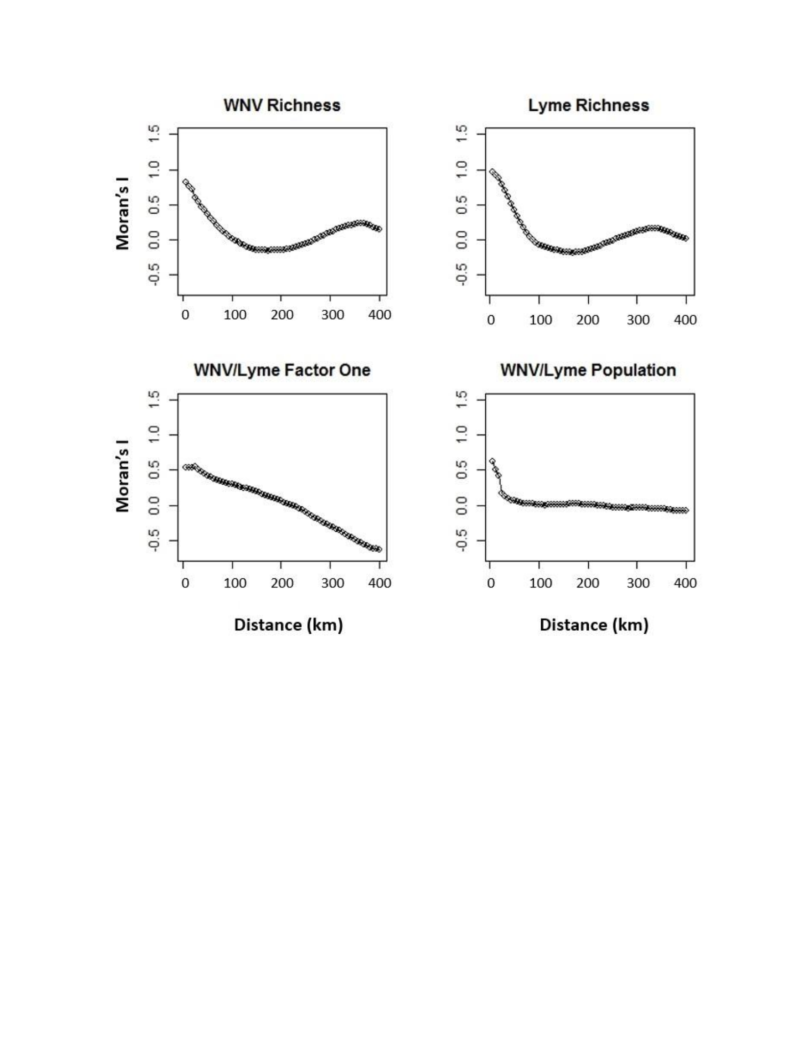
133
Figure A5. Spatial Correlograms. Correlograms of spatial autocorrelation (Moran’s I) as a
function of distance (degrees) for host richness, abiotic factor one (mainly representing
temperature), and human population data used in the GLS models. Autocorrelations for Bd
predictors should be interpreted with caution because geographic points were not evenly
distributed in space. Human population was moderately autocorrelated at first but quickly became
uncorrelated at short distances. Although host richness was initially highly autocorrelated, within
about a degree it became uncorrelated (except Bd). Factor one, which was the most commonly
significant factor in our models, remained autocorrelated for long distances. These correlograms

134
suggest that richness is highly variable (low autocorrelation) at smaller scales while abiotic
factors remain non-variable (autocorrelated), possibly providing an ecological explanation for our
model results.

135
Supplementary Tables
Table A1. Loadings from a factor analysis of eight abiotic variables, mean, minimum, and
maximum monthly temperature, precipitation, diurnal temperature range, annual
temperature range, altitude and NDVI, and associated variation accounted for by each
factor. Variables were condensed into four factors, three which were used to predict the
distribution of all three diseases across scales (in bold). Factor one was highly correlated with
temperature, factor two represents NDVI and precipitation, and factor three correlated with
temperature variability and altitude. Scores shown are from a factor analysis of climate variables
across the extent of the U.S. used to predict the spread of Batrachochytrium dendrobatidis.
However, the factor analysis performed for West Nile virus and Lyme disease, using climate
data in the Eastern U.S. only, produced nearly identical factors each representing the same
abiotic variables.
Table A2. Results of multi-model inference analyses (with shrinkage) predicting
the prevalence of West Nile virus and Borrelia burgdorferi. Models used host
richness, three abiotic factors, and human population density in the analysis.
Statistically significant (p<.05) values are in bold.
West Nile Virus Predictor
Coefficient
St. Error
z value
Pr(>|z|)
1/16th degree
Intercept
0.0060
0.0006
10.13
<0.001
Richness
0.0018
0.0009
2.04
0.042
Factor one
0.0006
0.0008
0.80
0.422
Factor two
0.0011
0.0007
1.51
0.132
Factor three
0.0001
0.0004
0.30
0.765
Population
<0.0001
0.0002
0.21
0.831
Coefficient 0.0060
St. Error
z value
Pr(>|z|)
Variables
Factor 1
Factor 2
Factor 3
Factor 4
Altitude
-0.478
-0.372
0.674
0.335
Annual Temp Variation
-0.449
-0.442
0.072
-0.640
Diurnal Temp Variation
0.075
-0.376
0.909
-0.149
NDVI
0.085
0.900
-0.246
0.079
Precipitation
0.158
0.773
-0.423
0.194
Mean Temperature
0.984
0.114
-0.076
0.107
Max Temperature
0.990
0.039
0.103
0.077
Min Temperature
0.941
0.183
-0.248
0.133
SS loadings
3.302
1.931
1.603
0.623
Proportion Variation
0.413
0.241
0.200
0.078
Cumulative Variation
0.413
0.654
0.855
0.932

136
1/8 degree
Intercept
0.0006
10.30
<0.001
Richness
0.0014
0.0010
1.32
0.189
Factor one
0.0008
0.0008
0.96
0.338
Factor two
0.0011
0.0007
1.46
0.144
Factor three
0.0004
0.0007
0.56
0.574
Population
<-0.0001
0.0002
0.22
0.829
1/4th degree
Intercept
Coefficient 0.0060
St. Error
z value
Pr(>|z|)
0.0006
10.45
<0.001
Richness
0.0010
0.0011
0.89
0.372
Factor one
0.0009
0.0009
1.00
0.315
Factor two
0.0010
0.0008
1.20
0.231
Factor three
0.0007
0.0009
0.83
0.407
Population
-0.0005
0.0006
0.75
0.456
½ degree
Intercept
Coefficient 0.0062
St. Error
z value
Pr(>|z|)
0.0006
10.50
<0.001
Richness
0.0001
0.0005
0.24
0.808
Factor one
0.0016
0.0008
2.03
0.043
Factor two
0.0004
0.0006
0.66
0.507
Factor three
0.0009
0.0008
1.08
0.279
Population
-0.0009
0.0008
1.08
0.280
1 degree
Coefficient
St. Error
z value
Pr(>|z|)
Intercept
0.0062
0.0006
10.56
<0.001
Richness
<-0.0001
0.0003
0.17
0.986
Factor one
0.0019
0.0007
2.64
0.008
Factor two
0.0002
0.0004
0.40
0.688
Factor three
0.0004
0.0006
0.59
0.554
Population
-0.0011
0.0009
1.29
0.196
Table A2 (continued)
2 degrees
Intercept
Coefficient
0.0066
St. Error
z value
Pr(>|z|)
0.0006
10.50
<0.001
Richness
0.0001
0.0004
0.26
0.794
Factor one
0.0019
0.0007
2.60
0.009
Factor two
<0.0001
0.0004
0.26
0.797
Factor three
0.0003
0.0006
0.46
0.645
Population
-0.0020
0.0009
2.16
0.031
4 degrees
Intercept
Coefficient 0.0067
St. Error
z value
Pr(>|z|)
0.0007
9.08
<0.001
Richness
0.0005
0.0009
0.57
0.567

137
Factor one
0.0012
0.0009
1.31
0.190
Factor two
0.0002
0.0006
0.37
0.712
Factor three
0.0010
0.0012
0.85
0.398
Population
-0.0021
0.0013
1.53
0.127
Lyme Disease Predictor
Coefficient
St. Error
z value
Pr(>|z|)
1/16th degree
Intercept
2.848
1.143
2.49
0.013
Richness
0.815
0.344
2.37
0.018
Factor one
-0.844
0.725
1.16
0.245
Factor two
0.246
0.376
0.65
0.513
Factor three
0.010
0.115
0.09
0.929
Population
-0.193
0.132
1.46
0.145
1/8 degree
Coefficient
St. Error
z value
Pr(>|z|)
Intercept
8.533
11.463
0.74
0.457
Richness
0.625
0.437
1.43
0.153
Factor one
-1.043
0.888
1.17
0.240
Factor two
0.109
0.301
0.36
0.716
Factor three
0.096
0.252
0.38
0.703
Population -0.409 0.132 3.08 0.002
1/4th degree
Coefficient
St. Error
z value
Pr(>|z|)
Intercept
6.884
9.434
0.73
0.466
Richness
0.120
0.256
0.47
0.638
Factor one
-0.366
0.723
0.51
0.613
Factor two
0.002
0.267
0.01
0.995
Factor three
0.188
0.295
0.64
0.524
Population
-0.648
0.161
4.03
<0.001
Table A2 (continued) ½
degree
Coefficient
St. Error
z value
Pr(>|z|)
Intercept
6.572
8.913
0.74
0.461
Richness
0.016
0.147
0.11
0.916
Factor one
-0.192
0.635
0.30
0.762
Factor two
-0.035
0.248
0.14
0.889
Factor three
0.287
0.340
0.84
0.399
Population
-0.529
0.278
1.90
0.058
1 degree
Coefficient
St. Error
z value
Pr(>|z|)

138
Intercept
6.253
8.103
0.77
0.441
Richness
-0.141
0.261
0.54
0.590
Factor one
0.260
0.587
0.44
0.658
Factor two
-0.169
0.309
0.55
0.585
Factor three
0.009
0.177
0.05
0.959
Population
-0.144
0.260
0.56
0.578
2 degrees
Coefficient
St. Error
z value
Pr(>|z|)
Intercept
4.467
6.550
0.68
0.496
Richness
-0.013
0.177
0.08
0.940
Factor one
0.552
0.864
0.64
0.523
Factor two
-1.412
0.553
2.70
0.007
Factor three
0.006
0.149
0.04
0.969
Population -0.770 0.526 1.46 0.143
4 degrees
Intercept
Richness
Factor one
Factor two
Factor three
Population
Coefficient
5.803
0.082
1.478
-0.893
0.004
0.131
St. Error
7.657
0.323
0.901
0.602
0.208
0.358
z value
0.76 0.54
2.43 2.28
0.05
0.92
Pr(>|z|)
0.449
0.588
0.015
0.023
0.961
0.360
Table A3. Effect of mosquito richness on West Nile virus distribution across scales.
Scale (degrees2)
Estimate
Std. Error
Adjusted SE
z value
Pr(>|z|)
0.0625
-2.92E-04
7.328E-04
7.33E-04
0.398
0.6905
0.125
-2.87E-04
7.723E-04
7.73E-04
0.372
0.710
0.25
-3.79E-05
4.128E-04
4.13E-04
0.092
0.927
0.5
1.713E-05
3.919E-04
3.92E-04
0.044
0.9652
1
2.833E-05
3.645E-04
3.65E-04
0.078
0.938
2
-1.97E-05
3.769E-04
3.77E-04
0.052
0.9584
4
-0.00025
0.0010168
0.001017
0.243
0.808

139
Table A4. Correlations between predictors across spatial scales.
Bd - 0.0625 degrees2
Factor One
Factor Two
Factor Three
Richness
Population
Factor One
1
0.369
-0.029
0.664
0.432
Factor Two
0.369
1
0.146
0.494
0.153
Factor Three
-0.029
0.146
1
-0.304
-0.421
Richness
0.664
0.494
-0.304
1
0.409
Population
0.432
0.152
-0.421
0.409
1
Bd - 0.125 degrees2
Factor One
Factor Two
Factor Three
Richness
Population
Factor One
1
0.361
-0.039
0.663
0.451
Factor Two
0.361
1
0.116
0.497
0.207
Factor Three
-0.039
0.116
1
-0.318
-0.468
Richness
0.663
0.497
-0.318
1
0.460
Population
0.451
0.207
-0.468
0.460
1
Bd - 0.25 degrees2
Factor One
Factor Two
Factor Three
Richness
Population
Factor One
1
0.345
-0.052
0.669
0.476
Factor Two
0.345
1
0.075
0.506
0.231
Factor Three
-0.052
0.075
1
-0.328
-0.514
Richness
0.669
0.506
-0.328
1
0.524
Population
0.476
0.231
-0.514
0.524
1
Bd - 0.5 degrees2
Factor One
Factor Two
Factor Three
Richness
Population
Factor One
1
0.335
-0.066
0.674
0.511
Factor Two
0.335
1
0.037
0.523
0.290
Factor Three
-0.066
0.037
1
-0.324
-0.586
Richness
0.674
0.523
-0.324
1
0.599
Population
0.511
0.290
-0.586
0.599
1

140
Table A4 (Continued)
Bd - 1 degrees2
Factor One
Factor Two
Factor Three
Richness
Population
Factor One
1
0.313
-0.093
0.660
0.510
Factor Two
0.313
1
-0.062
0.493
0.362
Factor Three
-0.093
-0.062
1
-0.330
-0.584
Richness
0.660
0.493
-0.330
1
0.632
Population
0.510
0.362
-0.584
0.632
1
Bd - 2 degrees2
Factor One
Factor Two
Factor Three
Richness
Population
Factor One
1
0.207
-0.168
0.693
0.498
Factor Two
0.207
1
-0.157
0.478
0.371
Factor Three
-0.168
-0.157
1
-0.358
-0.621
Richness
0.693
0.478
-0.358
1
0.673
Population
0.498
0.371
-0.621
0.673
1
Bd - 4 degrees2
Factor One
Factor Two
Factor Three
Richness
Population
Factor One
1
0.097
-0.227
0.638
0.518
Factor Two
0.097
1
-0.257
0.484
0.437
Factor Three
-0.227
-0.257
1
-0.422
-0.721
Richness
0.638
0.483
-0.422
1
0.743
Population
0.518
0.437
-0.721
0.743
1
WNV - 0.0625
degrees2
Factor One
Factor Two
Factor Three
Richness
Population
Factor One
1
0.042
-0.004
0.332
0.025
Factor Two
0.042
1
-0.118
-0.404
-0.211
Factor Three
-0.004
-0.118
1
0.524
0.111
Richness
0.332
-0.404
0.524
1
0.074
Population
0.025
-0.211
0.111
0.074
1

141
Table A4 (Continued)
WNV - 0.125 degrees2
Factor One
Factor Two
Factor Three
Richness
Population
Factor One
1
0.035
-0.002
0.333
0.018
Factor Two
0.035
1
-0.128
-0.433
-0.271
Factor Three
-0.002
-0.128
1
0.517
0.117
Richness
0.333
-0.433
0.517
1
0.112
Population
0.018
-0.271
0.117
0.112
1
WNV - 0.25 degrees2
Factor One
Factor Two
Factor Three
Richness
Population
Factor One
1
0.045
-0.008
0.331
-0.028
Factor Two
0.045
1
-0.137
-0.480
-0.368
Factor Three
-0.008
-0.137
1
0.521
0.121
Richness
0.331
-0.480
0.521
1
0.197
Population
-0.028
-0.368
0.121
0.197
1
WNV – 0.5 degrees2
Factor One
Factor Two
Factor Three
Richness
Population
Factor One
1
0.097
0.001
0.300
-0.044
Factor Two
0.097
1
-0.149
-0.496
-0.406
Factor Three
0.001
-0.149
1
0.513
0.095
Richness
0.300
-0.496
0.513
1
0.264
Population
-0.044
-0.406
0.095
0.264
1
WNV - 1 degrees2
Factor One
Factor Two
Factor Three
Richness
Population
Factor One
1
0.189
0.047
0.259
-0.091
Factor Two
0.189
1
-0.172
-0.477
-0.390
Factor Three
0.047
-0.172
1
0.502
0.035
Richness
0.259
-0.477
0.502
1
0.309
Population
-0.091
-0.390
0.035
0.309
1
Table A4 (Continued)
WNV - 2 degrees2
Factor One
Factor Two
Factor Three
Richness
Population

142
Factor One
1
0.260
0.100
0.226
-0.124
Factor Two
0.260
1
-0.166
-0.430
-0.349
Factor Three
0.100
-0.166
1
0.544
-0.055
Richness
0.226
-0.430
0.544
1
0.317
Population
-0.124
-0.349
-0.055
0.317
1
WNV - 4 degrees2
Factor One
Factor Two
Factor Three
Richness
Population
Factor One
1
0.362
0.223
0.227
-0.189
Factor Two
0.362
1
-0.184
-0.161
-0.368
Factor Three
0.223
-0.185
1
0.513
-0.157
Richness
0.227
-0.161
0.513
1
0.293
Population
-0.190
-0.368
-0.157
0.293
1
Lyme – 0.0625 degrees2
Factor One
Factor Two
Factor Three
Richness
Population
Factor One
1
0.047
-0.006
-0.107
0.023
Factor Two
0.047
1
-0.115
0.455
-0.206
Factor Three
-0.006
-0.115
1
-0.641
0.109
Richness
-0.107
0.455
-0.641
1
-0.065
Population
0.023
-0.206
0.109
-0.065
1
Lyme – 0.125 degrees2
Factor One
Factor Two
Factor Three
Richness
Population
Factor One
1
0.040
-0.004
-0.110
0.015
Factor Two
0.040
1
-0.125
0.463
-0.265
Factor Three
-0.004
-0.125
1
-0.648
0.115
Richness
-0.110
0.463
-0.648
1
-0.075
Population
0.015
-0.265
0.115
-0.075
1
Table A4 (Continued)
Lyme – 0.25 degrees2
Factor One
Factor Two
Factor Three
Richness
Population

143
Factor One
1
0.045
-0.008
-0.102
-0.028
Factor Two
0.045
1
-0.137
0.472
-0.368
Factor Three
-0.008
-0.137
1
-0.657
0.121
Richness
-0.102
0.472
-0.657
1
-0.116
Population
-0.028
-0.368
0.121
-0.116
1
Lyme – 0.5 degrees2
Factor One
Factor Two
Factor Three
Richness
Population
Factor One
1
0.097
0.001
-0.083
-0.044
Factor Two
0.097
1
-0.149
0.492
-0.406
Factor Three
0.001
-0.149
1
-0.664
0.095
Richness
-0.083
0.492
-0.664
1
-0.103
Population
-0.044
-0.406
0.095
-0.103
1
Lyme - 1 degrees2
Factor One
Factor Two
Factor Three
Richness
Population
Factor One
1
0.189
0.047
-0.081
-0.091
Factor Two
0.189
1
-0.172
0.523
-0.390
Factor Three
0.047
-0.172
1
-0.628
0.035
Richness
-0.081
0.523
-0.628
1
-0.024
Population
-0.091
-0.390
0.035
-0.024
1
Lyme - 2 degrees2
Factor One
Factor Two
Factor Three
Richness
Population
Factor One
1
0.260
0.100
-0.104
-0.124
Factor Two
0.260
1
-0.166
0.546
-0.349
Factor Three
0.100
-0.166
1
-0.518
-0.055
Richness
-0.104
0.546
-0.518
1
0.178
Population
-0.124
-0.349
-0.055
0.178
1
Table A4 (Continued)
Lyme - 4 degrees2
Factor One
Factor Two
Factor Three
Richness
Population
Factor One
1
0.362
0.223
-0.169
-0.189

144
Factor Two
0.362
1
-0.184
0.435
-0.368
Factor Three
0.223
-0.184
1
-0.446
-0.157
Richness
-0.169
0.435
-0.446
1
0.400
Population
-0.189
-0.368
-0.157
0.400
1

145
Table A5. Raw root mean square error (RMSE) of each model output for every other scale
in our analyses as well as RMSE standardized to the range of values in the response
variables. RMSE represents the mean deviation between the observed and predicted values of the
statistical model and thus smaller values indicate better overall fit of the model to the data. There
were no scale-dependent patterns of RMSE across disease systems. Units for RMSE are as
follows: for Bd, arcsine-transformed prevalence; and for West Nile virus and Lyme disease, cases
per 10,000 people. Standardized RMSE values are unitless proportions.
Root mean standard error (RMSE)
Standardized RMSE
Scale
Bd West Nile Lyme
Virus Disease
Bd
West Nile Lyme Virus
Disease
0.0625 degrees2
0.4215
0.0746
0.0517
0.268
0.037
0.0005
0.25 degrees2
0.4226
0.0744
0.0740
0.269
0.037
0.0007
1 degree2
0.4237
0.0745
0.0716
0.270
0.037
0.0007
4 degrees2
0.4260
0.0743
0.0718
0.271
0.037
0.0007

146
West Nile virus
(
scale,
degrees
2
)
0.0625
0.125
1
2
4
0
Table A6. Complete list of models used in model averaging with their ΔAkaike scores.
Chytrid (scale, degrees2)
0.0625
0.125
0.25
0.5
1
2
4
Intrc,Factor3,Factor2,Rich
0.87
3.85
5.68
12.1
9.46
13.59
Intrc,Factor1,Factor3,Rich
1.29
1.09
0.75
6.96
10.97
7.91
12.78
Intrc,Factor2,Rich
1.71
1.82
6.91
8.31
17.94
23.95
31.29
Intrc,Rich
1.86
3.55
7.51
12.31
24.6
24.56
31.23
Intrc,Factor1,Rich
1.99
1.36
3.98
8.93
17.81
23.95
31.94
Intrc,Factor1,Factor2,Rich
2.09
0
3.47
4.61
10.78
22.05
30.51
Intrc,Factor3,Rich
2.26
4.62
6.76
12.25
20.85
10.39
12.82
Intrc,Factor3,Rich,Pop
3.08
6.24
8.42
13.66
21.92
1.81
2.87
Intrc,Factor1,Rich,Pop
3.12
2.93
5.9
10.83
17.2
2.47
3.5
Intrc,Factor2,Rich,Pop
3.47
3.81
8.88
10.3
16.51
2.72
3.52
Intrc,Rich,Pop
3.52
5.52
9.5
14.32
22.33
2.29
1.96
Intrc,Factor1,Factor3,Factor2
11.71
3.64
0
0
0
4.53
11.42
Intrc,Factor1,Factor3,Pop
27.84
20.89
14.14
20.61
17.11
0
2.11
Intrc,Factor1,Factor3
28.86
20.47
13.53
19.5
15.72
12.12
16.18
Intrc,Factor1,Factor2
31.73
18.98
18.38
14.16
14.49
27.45
35.13
Intrc,Factor1,Factor2,Pop
33.66
20.74
19.32
15.13
11.51
0.12
2.78
Intrc,Factor3,Factor2,
37.55
31.11
30.26
26.65
26.42
23.65
21.73
Intrc,Factor3,Factor2,Pop
39.5
32.8
31.32
27.83
23.24
2.8
2.44
Intrc,Factor1,
42.66
31.14
28.42
31.15
31.09
39.19
48.39
Intrc,Factor1,Pop
44.61
32.65
28.71
30.44
22.72
1.47
1.49
Intrc,Factor2,Pop
57.27
44.39
42.3
34.19
25.98
3.21
1.5
Intrc,Factor2
61.88
50.31
52.73
44.32
44.19
53.5
54.56
Intrc,Factor3,Pop
79.97
69.89
60.91
60.48
43.01
4.99
1.08
Intrc,Factor3
81.48
74.28
67.27
70.35
61.37
37.55
27.21
Intrc,Pop
86.52
72.53
64.22
60.19
42.57
4.8
0
Intrc
96.24
86.48
84.67
85.13
81.88
75.05
71.38
0.25 0.5
Intrc,Factor1,Factor2,Rich 0 0.73 4.58 5.18 8.23 7.89
Intrc,Factor2,Rich
0.72
0.78
1.11
7.17
10.42
13.49
10.79
Intrc,Factor2,Pop,Rich
2.22
2.61
0.58
5.93
8.25
7.11
4.46
Intrc,Factor3,Factor2,Rich
2.68
2.33
2.25
7.93
11.53
14.47
6.74
Intrc,Factor1,Rich
4.12
5.21
8
8.41
5.19
7.95
7.36
Intrc,Factor1,Factor3,Factor2
4.45
1.7
0.49
1.76
3.39
6.71
3.24
Intrc,Factor1,Factor3,Rich
4.88
4.64
6.16
6.08
4.56
7.86
5.67
Intrc,Factor1,Factor3
5.06
3.34
4.16
4.79
4.1
6.87
3.74
Intrc,Rich
5.22
6.44
9.23
12.54
12.6
15.87
12.26
Intrc,Factor1,Pop,Rich
6
6.44
4.91
4.74
2.11
1.44
0.43

147
Intrc,Factor3,Rich
6.83
7.22
9.17
12.39
13.35
16.5
9.58
Table A6 (continued)
West Nile virus (scale,
degrees2)
0.0625
6.92
0.125
0.25
0.5
1
2
4
Intrc,Factor1,Factor2
5.08
4.4
3.98
3.19
6.28
6.6
Intrc,Factor1,Factor3,Pop
7.04
4.11
0
0
0
0.57
0
Intrc,Pop,Rich
7.05
7.76
6.02
8.45
8.45
7.45
3.3
Intrc,Factor1
7.45
6.54
7.57
6.42
3.47
6.04
5.81
Intrc,Factor1,Factor2,Pop
8.34
6.97
4.41
3.33
1.57
1.74
3.6
Intrc,Factor3,Pop,Rich
8.73
8.24
5.04
7.82
9.28
9.02
3.65
Intrc,Factor1,Pop
9.17
8.08
5.56
3.28
0.13
0
1.7
Intrc,Factor3
12.02
9.38
8.92
10.57
11.34
14.49
7.59
Intrc,Factor3,Factor2
12.31
8.84
6.48
8.19
10.12
12.9
4.75
Intrc
13.78
11.98
11.84
11.93
10.9
14.35
12.17
Intrc,Factor3,Pop
13.85
10.59
5.54
6.71
7.75
8.33
3.68
Intrc,Factor3,Factor2,Pop
13.95
10.47
5.21
6.88
8.59
9.02
3.44
Intrc,Factor2
14.12
11.57
9.81
10.1
10.19
13.38
11.14
Intrc,Pop
15.23
13.75
10.42
9.6
8.15
8.59
7.83
Intrc,Factor2,Pop
15.25
13.53
10.02
9.87
9.22
9.62
8.79
0.25 0.5
Intrc,Factor1,Rich,Pop 0 1.27 4.36 1.58 7.09 5.01
Intrc,Factor2,Rich,Pop
1.68
2.95
2.88
5.47
1.25
2
6.84
Intrc,Factor2,Rich
4.39
10.21
15.47
8.47
1.25
5.72
5.06
Intrc,Factor1,Rich
4.43
10.03
15.95
7.51
0.97
7.42
5.34
Intrc,Factor1,Factor2,Rich
5.24
11.58
17.43
9.45
2.94
5.09
0.89
Intrc,Factor3,Rich,Pop
5.69
2.68
0.42
1.78
3.12
16.38
11.09
Intrc,Factor1,Factor3,Rich
6.06
11.2
17.28
9.28
2.98
9.35
7.17
Intrc,Factor3,Factor2,Rich
6.23
11.91
17.48
9.31
3.08
7.38
7.01
Intrc,Factor1,Pop
6.69
3.63
0.3
2.35
1.21
7.34
3.91
Intrc,Rich,Pop
7.76
6.77
1.68
3.51
1.23
14.54
9.08
Intrc,Factor1,Factor2,Pop
8.13
5.59
1.61
2.86
1.99
0.01
1.43
Intrc,Factor2,Pop
8.21
6
1.83
3.45
0
0
4.93
Intrc,Factor1,Factor3,Pop
8.41
5.65
1.69
1.99
2.19
7.26
5.64
Intrc,Factor3,Factor2,Pop
9.91
6.25
1.8
1.97
1.88
2.01
6.94
Intrc,Factor2
10.95
12.98
14.19
6.47
0.09
3.94
3.5
Intrc,Factor1
11.29
13.46
14.96
5.5
0.37
8.29
3.65
Intrc,Factor1,Factor2
11.74
14.62
16.19
7.45
1.96
3.32
0
Lyme disease
(
scale,
degrees
2
)
0.0625
0.125
1
2
4
0

148
Intrc,Factor1,Factor3
11.94
14.07
16.01
7.31
2.08
9.34
5.25
Intrc,Factor3,Rich
12.29
16.31
18.69
7.99
1.88
15.75
12.14
Intrc,Rich
12.54
16.88
17.02
7.63
0.19
14.36
10.41
Intrc,Factor3,Factor2
12.96
14.89
16.21
7.34
2.1
5.77
5.51
Intrc,Factor1,Factor3,Factor2
13.02
15.9
18.02
9.31
3.91
5.31
1.98
Table A6 (continued)
Lyme disease (scale,
degrees2)
0.0625
0.125
0.25
0.5
1
2
4
Intrc,Factor3,Pop
7.33
0
0
3.32
20.59
11.04
Intrc,Pop
15.8
10.44
0.89
1.5
1.34
18.82
9.91
Intrc
20.84
20.36
16.23
5.65
0.04
19.46
10.02
Intrc,Factor3
21.59
20.35
17.99
6.21
2.05
21.46
10.9

149
Table A7. Model averaged outputs without shrinkage. We caution that parameter estimates
with shrinkage are most appropriate. In multiple regression analyses, estimates with shrinkage are
preferable because they reduce model selection bias. Please see Supplemental Results for
additional details.
Chytrid
West Nile virus
Lyme disease
0.0625 degrees2
Estimate
Std. Error
Estimate
Std. Error
Estimate
Std. Error
(Intercept)
0.59897
0.02518
0.005954
0.000587
2.8476
1.1431
FactorThree
0.03774
0.02279
0.000657
0.000807
0.114
0.3664
FactorTwo
-0.04428
0.02681
0.001331
0.000552
0.6954
0.2958
Richness
-0.16387
0.0277
0.002047
0.000693
0.8609
0.2913
FactorOne
-0.03221
0.02191
0.001248
0.00071
-1.2954
0.4731
Population 0.01565 0.01989 0.000255 0.000415 -0.2416
0.1004
0.125 degrees2 Estimate Std. Error Estimate Std. Error Estimate Std. Error
(Intercept)
0.6029
0.02816
0.00603
0.000585
8.5334
11.4639
FactorOne
-0.04791
0.02453
0.001408
0.000714
-1.5729
0.5968
FactorTwo
-0.05407
0.02874
0.001358
0.000567
0.5381
0.4643
Richness
-0.13988
0.02965
0.001848
0.000725
0.7923
0.3325
FactorThree
0.03941
0.02697
0.001111
0.000746
0.4725
0.3667
Population
0.00887
0.02014
-0.0003
0.000471
-0.4144
0.1239
0.25 degrees2
Estimate
Std. Error
Estimate
Std. Error
Estimate
Std. Error
(Intercept)
0.58405
0.027387
0.006149
0.000588
6.8836
9.4349
FactorOne
-0.078
0.028254
0.001498
0.000673
-0.9976
0.893
FactorThree
0.071878
0.029836
0.00143
0.000697
0.4409
0.3048
FactorTwo
-0.07785
0.030451
0.001499
0.000605
0.0068
0.5432
Richness
-0.11828
0.031421
0.001837
0.000768
0.3715
0.3301
Population
0.005455
0.022396
-0.0011
0.000562
-0.6482
0.16

150
0.5 degrees2 Estimate Std. Error Estimate Std. Error Estimate Std. Error
(Intercept)
0.600056
0.025625
0.006153
0.000586
6.5718
8.9133
FactorOne
-0.08917
0.022474
0.001764
0.000618
-0.659
1.0358
FactorThree
0.079372
0.022955
0.001346
0.000621
0.512
0.3009
FactorTwo
-0.09939
0.026935
0.001126
0.000589
-0.1445
0.4895
Richness
-0.11178
0.031444
0.000718
0.000946
0.0738
0.3142
Population
0.002044
0.02523
-0.00144
0.000626
-0.5856
0.2293
Table A7 (Continued)
1 degree2 Estimate Std. Error Estimate Std. Error Estimate Std.
Error
(Intercept)
0.59527
0.02388
0.006207
0.000587
6.25332
8.10282
FactorOne
-0.09717
0.0184
0.001963
0.000632
0.72918
0.79049
FactorThree
0.0906
0.02237
0.000948
0.00066
0.03594
0.35137
FactorTwo
-0.09491
0.02261
0.000693
0.000637
-0.4161
0.3645
Richness
-0.07604
0.02968
-3.4E-05
0.000818
-0.36364
0.30804
Population
- 0.05145
0.02576
-0.00154
0.000669
-0.35687
0.30119
(Intercept)
0.60158
0.02548
0.00664
0.000632
4.46738
6.55022
FactorOne
-0.05069
0.02347
0.002003
0.000641
1.30635
0.88405
FactorThree
0.05807
0.03519
0.000889
0.000731
0.03606
0.36851
Population
-0.13511
0.03268
-0.00219
0.000775
-0.95509
0.40791
FactorTwo
-0.0447
0.02547
0.000507
0.000727
-1.47287
0.44334
Richness
- 0.04954
0.03013
0.00052
0.000771
-0.07892
0.42442
4 degrees2
Estimate
Std. Error
Estimate
Std. Error
Estimate
Std. Error
(Intercept)
0.58735
0.021208
0.006747
0.000743
5.80359
7.65677

151
2 degrees2 Estimate Std. Error Estimate Std. Error Estimate Std.
Error
Supplementary References
Ciota, A. T. and L. D. Kramer (2013). "Vector-Virus Interactions and Transmission Dynamics of
West Nile Virus." Viruses-Basel 5(12): 3021-3047.
Heaney, L. R. (2000). "Dynamic disequilibrium: a long-term, large-scale perspective on the
equilibrium model of island biogeography." Global Ecology and Biogeography 9(1): 59-
74.
Hijmans, R. J. (2014). "raster: Geographic data analysis and modeling, R package version
2.2.31."
O'Brien, R. M. (2007). "A caution regarding rules of thumb for variance inflation factors."
Quality & Quantity 41(5): 673-690.
Sexton, J. P., P. J. McIntyre, et al. (2009). "Evolution and Ecology of Species Range Limits."
Annual Review of Ecology Evolution and Systematics 40: 415-436.
Team, R. C. (2014). R: A language and environment for statistical computing. R Foundation for
Statistical Computing, Vienna, Austria.
Population
-0.17725
0.033129
-0.00254
0.001047
0.50565
0.55191
FactorThree
0.038727
0.037242
0.001974
0.000997
0.02379
0.48549
FactorOne
-0.01927
0.023562
0.00161
0.000684
1.73403
0.71411
FactorTwo
-0.02039
0.026687
0.000997
0.00089
-1.08988
0.47805
Richness
-0.00594
0.030468
0.001458
0.000984
0.30624
0.56466

152
Appendix B: Supplementary Materials: Chapter Three
Supplementary Methods
Literature survey and data requirements
We conducted a literature search in September 2012 on Web of Science for the term
“phenology climate” within the following fields: environmental sciences and ecology, zoology,
developmental biology, reproductive biology, life sciences (other), entomology, behavioral
sciences, physiology, biodiversity and conservation, fisheries, evolutionary biology, parasitology,
marine and freshwater biology, infectious diseases, and oceanography. This search generated
6,989 studies which were examined for phenological time series. References in these papers and
the USA National Phenology Network (usanpn.org) database were also examined for time series.
Time series were not used if they (1) contained data from a span of <10 years; (2) contained data
for fewer than seven individual years; (3) described autumn migrations; or (4) described data that
was redundant with data we had already compiled from another paper. We also eliminated raw
data from before 1950, because this is considered to be before significant global climate change
(Pachauri, Allen et al. 2014). Our exclusion criteria are similar to those from previous
metaanalyses (Parmesan and Yohe 2003; Root, Price et al. 2003).
Data extractions
We extracted raw time series data from figures plotting Julian date of phenological event
against year using Datathief III Version 1.6 (© Bas Tummers) (Tummers 2006). Correlation
coefficients, standard errors or surrogates, and slopes were also calculated for each time series
when they were not reported in the original text (All analyses were conducted in R 3.1.0 (2014)
(Team 2014); stats package, glm function). Correlation coefficients (r) and standard deviations

153
were available for 1,011 of these time series (representing 127 studies), which were included in
the random-effects meta-analysis synthesizing the correlations between phenology and time.
Approximately 400 time series from about 100 papers provided raw data and were used in the
meta-analyses examining the relationships between phenology, year, and climate (the actual
numbers varied between different climate variables because some variables were not available at
certain geographic locations). All correlation coefficients and their sampling variances (used as
weights) were standardized using Fisher’s z-transformation before all meta-analysis modeling.
External climate data
Climate data were downloaded from the NOAA National Climatic Data Center (NCDC
(Lawrimore, Menne et al. 2011); www.ncdc.noaa.gov) worldwide database of “monthly
observational data” corresponding to the nearest location (within 100km) and full time span of
every time series that provided raw data and geographic coordinates. Ten climate variables were
used in the analysis (see Fig. S3), and they generally were related to temperature or precipitation.
Yearly averages of climate variables were compiled for all variables in all locations and for the
years in all time series only when data were available for all 12 months. Within each time series,
correlation coefficients and standard errors were compiled for all correlations between annual
climate variables and both phenology and year (stats package (Team 2014), glm function).
Independent fixed-effects variables
Independent variables collected for each time series included taxonomic classification of
the focal species, absolute value of latitude, elevation, metabolic strategy (ectothermy or
endothermy), trophic level, habitat (terrestrial or marine), log-transformed body mass (see below)
and type of phenological event (endpoint). Taxonomic classification was assessed to the class

154
level. Elevation specific to the locations where time series were observed was extracted from
Worldclim elevation rasters (Hijmans, Cameron et al. 2005) (www.worldclim.org) (raster package
(Hijmans 2014), extract function). Trophic levels were assigned categorically as
“herbivore”, “omnivore”, or “carnivore”. If a species mostly relied on either prey or plants but
occasionally ate the other, it was assigned to “carnivore” or “herbivore” respectively.
Phenological events were categorized as either “arrival” (migrations), “breeding/rearing” (calling,
nesting, laying, hatching, or weaning), or “abundance” (peak population abundance).
Species-level body mass data
We collected species-level body masses from several existing datasets and other sources
(Dunning Jr 1992; Karlsson 1995; Garcia-Barros 2000; Williams and MacGowan 2004; Brose,
Cushing et al. 2005; Jones, Bielby et al. 2009; Dell, Pawar et al. 2011; Trochet, Moulherat et al.
2014; Myers 2016). We calculated mass based on body length for some insect species as
described by Chown et al. (Chown, Marais et al. 2007) and Hodar et al. (Hódar 1997) when we
could not find published estimates of body mass. For species for which we could not obtain or
calculate reliable body mass data, we estimated mass by taking the mean of the mass of species in
the lowest taxonomic level occupied by that species. Although this method is relatively coarse,
we were not concerned about obtaining highly specific values of mass because across the
organisms in our dataset, mass varied by >10 orders of magnitude, and mass was log-transformed
in our analyses.
Meta-analysis models
Using the full dataset, we conducted a standard meta-analysis (including random effects
modeled as between-study variance and phylogeny) to calculate the effect of time on phenology.

155
For time series where climate data were available, a trivariate random-effects meta-analysis was
used to jointly analyze the three effect sizes quantifying the three pairwise relationships among
phenology, time, and climate. Preserving the trivariate structure of effect sizes has the advantage
of accounting for the correlations within the three non-independent effect sizes (because of
sampling variability and covariances), while also explicitly accounting for any existing
correlations among these three effect size groups (via a multivariate random-effects model). Our
overall model had a hierarchical structure in which we modeled the correlations among the effect
size triplicates (within-study modeling for sampling variability), unstructured random-effects for
each effect size group that were allowed to be correlated but differ among groups, an unstructured
random-effects modeling the phylogenetic correlations among taxa, and finally a between-study
model that accounted for the overall between-study variance typical for a traditional
randomeffects meta-analysis. For all models, the rma.mv function from the R package metafor
was used (Viechtbauer 2010), with the variance-covariance matrix as the variance-covariance
matrix of the sampling errors, and all three random effects (trivariate structures, overall between-
study variance, and phylogenetic) were based on restricted maximum likelihood estimator using a
nlminb numerical optimizer. However, we did not include phylogenetic random-effects in our
analyses of the relationship between phenology and body size because phylogeny and body size
are highly correlated and thus controlling for phylogeny also indirectly eliminates much of the
body size variation. To plot the relationship between body mass and phenology, we used the
ggplot2 package, ggplot function (Wickham 2009). Please see Supplementary Code for examples
of the code used in these analyses.

156
Non-independence due to common variables among multiple effect sizes
We accounted for the non-independence that occurs when combining and comparing
multiple correlations that share common variables (phenology date, climate, and year) by
including their estimated sampling covariances in the off-diagonals of the variance-covariance
(VCV) matrix used as weights for meta-analyses and meta-regressions (sensu Lajeunesse
(Lajeunesse 2011)). This VCV matrix has a block-diagonal design, where each block represents a
3 by 3 matrix where the main diagonal contains the sampling variances (var) of each of three
Fisher’s Z transformed correlation (effect size), or:
var(Zjk) = var(Zjm) = var(Zkm) = n −13,
where each variance is the predicted sampling variance of the pairwise Fisher’s Z transformed
correlation for three variables j (time), k (phenology), and m (climate). All correlations share a
common sample size (𝑛). The covariance between two Z correlations, for example Zjk and Zjm, is
cov(Zjk, Zjm), where Zjk is the effect size for a correlation between variables j and k, and Zjm is the
effect size for the correlation between j and m. Further, the raw (Pearson product moment)
correlations are also used to estimate covariances, where for example between j and k the
correlation will be ρjk. Following Olkin and Finn (Olkin and Finn 1995) and Becker (Becker
2000), the covariance between two Fisher’s Z correlation with a common variable, cov(Zjk, Zjm),
is estimated as:
cov(Zjk, Zjm) .
jk jm

157
The covariance was estimated for all pairwise correlations among the phenology, time, and
climate variables. For example, the VCV for the effect size triplicates can be described with the
following symmetric matrix:
var(Zjk) cov(Zjk, Zjm) cov(Zjk, Zkm)
VCV = [ var(Zjm) cov(Zjm, Zkm)].
var(Zkm)
These VCV matrices were then stacked diagonally into a single matrix for meta-analysis. When
needed, individual VCV matrices that were not positive definite were fixed following Higham
(Higham 2002).
Non-independence due to shared evolutionary history among taxa
To account for the correlational structures among taxa due to their shared evolutionary
history (Lajeunesse 2009), we treated the phylogenetic correlations derived from a composite
phylogenetic tree of all taxa in our study (described below) as an unstructured random-effect in
our trivariate meta-regressions. These phylogenetic correlations were extracted from our
ultrametric tree using the vcv() function of the ape package in R (Paradis, Claude et al. 2004), and
explicitly assume trait evolution via Brownian Motion (Grafen 1989). Our composite phylogeny
of all 475 species used the topology and inter-node divergence times from published sources
when available (Fig. S1). The deep divergence times among phyla were based on Hedges et al.
(Hedges, Dudley et al. 2006). Among vertebrates, the topology and estimated divergence times
among fish were compiled from Betancur-R. et al. (Betancur-R, Broughton et al. 2013), mammals
from Meredith et al. (Meredith, Janecka et al. 2011), and amphibians from Shaffer and McKnight
(Shaffer and McKnight 1996) and Moriarty and Cannatella (Moriarty and Cannatella 2004). The
topology and divergence times among birds was derived from a random sample of the Bayesian

158
tree pool provided by the online avian phylogeny generating tool (Jetz, Thomas et al. 2012).
Among invertebrates, the topology and divergence times among hexapods, calanoids, and
branchiopods were based on Podar et al. (Podar, Haddock et al. 2001) and Regier et al. (Regier,
Mitter et al. 2013). The topology and divergence times among insect orders were compiled using
Trautwein et al. (Trautwein, Wiegmann et al. 2012). However, within insect orders only
topologies were available for moths and butterflies (Freitas and Brown 2004; Wahlberg et al.
2005a; (Freitas and Brown 2004; Wahlberg, Braby et al. 2005; Regier, Mitter et al. 2013)), and
dragonflies and damselflies (Dumont, Vierstraete et al. 2010). Since the divergence times within
Lepidoptera and Odonata were unavailable, we arbitrarily scaled branchlengths distances using
Grafen’s (Grafen 1989) method while assuming ρ to the power of 1.0 to create divergence times
fitting a Brownian motion model of evolution.

159
Supplementary Figures
Figure B1. Shifts in climate variables over time. Temperature shifted more over time than
precipitation in areas where phenology time series were recorded in studies. Because recent major
shifts in temperature have occurred alongside phenological advancements, the two phenomena
have been closely associated with each other. Error bars represent standard errors.
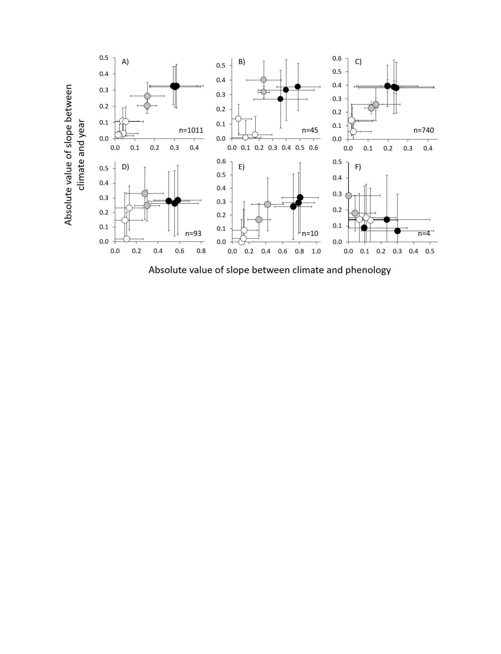
160
Figure B2. Generality of climatic conditions influencing changes in phenology. Absolute
values of grand means of slopes between phenology and climate (x-axis) and between climate
and time (y-axis) for the ten climatic variables used in the analysis (points). Variables that
changed over time and were predictive of animal phenology appear in the upper right-hand
corner, while variables that did not change much over time and did not match animal phenology
well appear in the lower-left corner. Error bars represent standard errors for the regression slope
parameters. We plotted absolute values to highlight the magnitude (rather than the direction) of
the effect, because different climate variables affect phenology in different directions. We found a
strong relationship between temperature variables (black circles) and phenology for (a) all taxa,
(b) amphibians, (c) birds, and (d) butterflies. Relationships between temperature and phenology
for (e) non-insect invertebrates and (f) mammals are presented as well. Meanwhile, relationships
between phenology and precipitation variables (white circles) and precipitation and time were
generally weaker than relationships between phenology and temperature variables and
temperature and time, respectively. Of all the taxonomic groups, only amphibians had a
significant relationship between precipitation (white circles) and phenology, but precipitation was
still a weaker predictor of amphibian phenology than temperature. Gray circles represent
variables derived from temperature (see methods for a list of variables in each category).
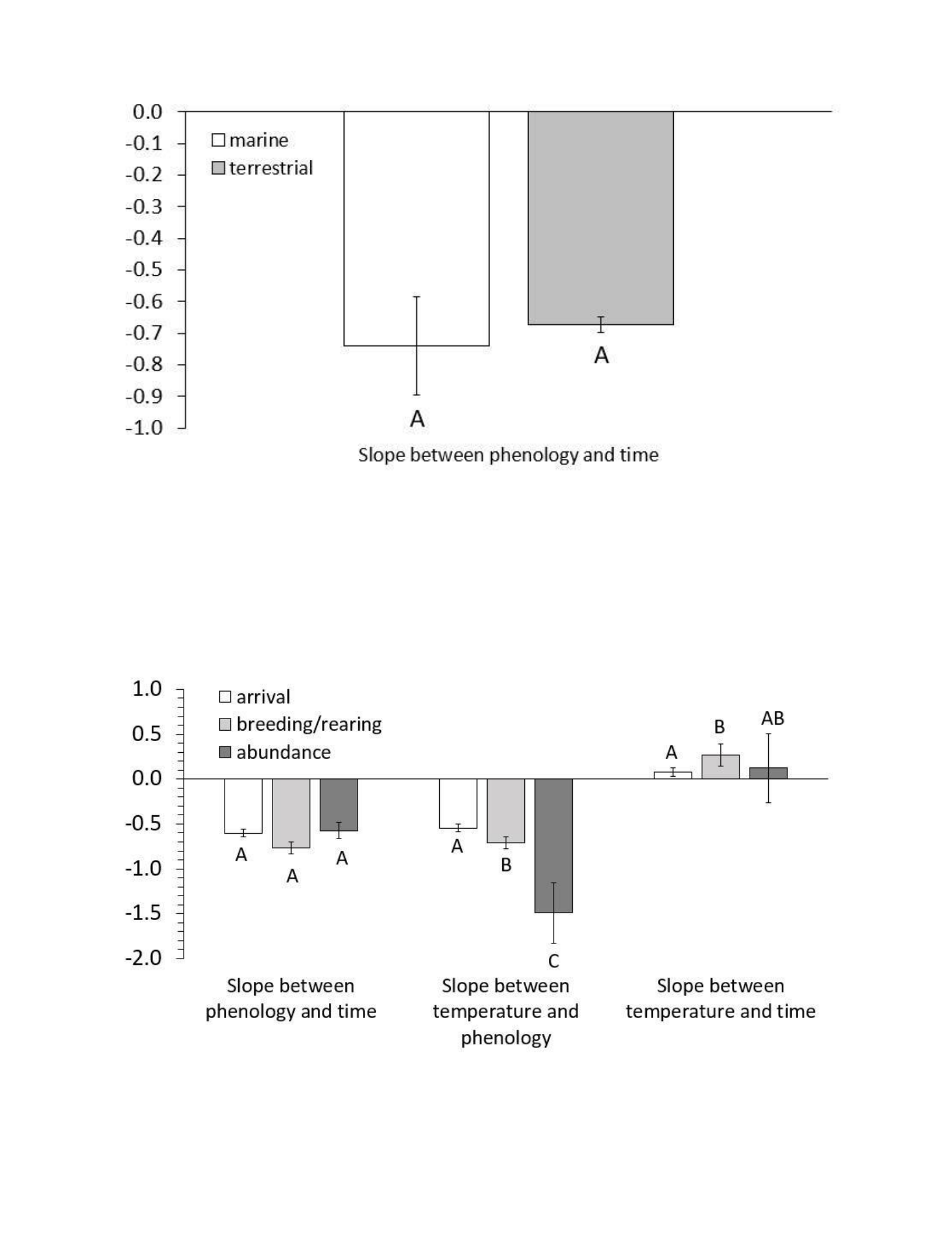
161
Figure B3. Phenological shifts in terrestrial and marine species. We categorized habitat type
as terrestrial or marine. We could only examine how the relationship between phenology and time
differed between habitat type because we did not have climate data for marine species.
Controlling for body size, there was no difference between phenological shifts between terrestrial
and marine species. Error bars represent standard errors for the slope parameters.
Figure B4. Phenological endpoints respond differently to climate change. We categorized
phenological endpoints as associated with either “arrival” (migration), “breeding/rearing”

162
(calling, nesting, laying, hatching, weaning), or “abundance” (time of peak abundance).
Controlling for body size, abundance phenology tracked temperature change more closely than
arrival or breeding/rearing endpoints. Breeding/rearing phenology was more closely tied to
temperature than arrival phenology, possibly because arrival phenology is dependent on the
climatic conditions in the region from where the species was overwintering, which were not
included in the analyses. Error bars represent standard errors for the slope parameters.

arrival arrival arrival
163
Supplementary Tables
(Abraham and Sydeman 2004)
breeding
1
Aves
USA
1973-
2001
5.17
(Adamik and Pietruszkova
2008)
arrival
1
Aves
Czech
Republic
1964-
2004
-2.02
(Adamik and Pietruszkova
2008)
arrival
1
Aves
Czech
Republic
1964-
2004
-2.64
(Ahas 1999)
arrival
1
Aves
Estonia
1952-
1996
-2.89
(Ahola, Laaksonen et al. 2004)
arrival
1
Aves
Finland
1970-
2002
-2.66
(Ahola, Laaksonen et al. 2004)
arrival
1
Aves
Finland
1970-
2002
-1.16
(Ahola, Laaksonen et al. 2004)
breeding
1
Aves
Finland
1970-
2002
0.35
(Anthes 2004)
arrival
1
Aves
Germany
1969-
2002
-2.95
(Askeyev, Sparks et al. 2007)
arrival
4
Aves
Russia
1957-
2004
-0.46
(Askeyev, Sparks et al. 2009)
arrival
1
Aves
Russia
1950-
2008
-1.49
(Askeyev, Sparks et al. 2009)
arrival
4
Aves
Russia
1957-
2008
-0.94
(Barbraud and Weimerskirch
2006)
arrival
9
Aves
Antarctica
1951-
2005
2.48
(Barbraud and Weimerskirch
2006)
breeding
5
Aves
Antarctica
1953-
2001
0.24
(Barrett 2002)
arrival
2
Aves
Norway
1978-
2000
-0.35
(Bauer, Trnka et al. 2010)
breeding
2
Aves
Czech
Republic
1961-
2007
-1.89
(Bauer, Trnka et al. 2010)
arrival
1
Insecta
Czech
Republic
1961-
2007
-1.61
(Beaumont, McAllan et al.
2006)
16
Aves
Australia
1960-
2004
-7.25

Table B1 (continued)
( Aves
arrival arrival arrival
164
Paper
Event
N
Class
Country
Time
Span
S
hift
Table B1. List of studies and time-series collected for meta-analysis. Papers were included in
the meta-analysis if they satisfied the basic requirements detailed in Methods and provided raw
time-series data on phenological date. Papers were included in the trivariate meta-analysis
(including climate in models) if they were at specific sites with locally corresponding terrestrial
NOAA climate data (papers not included are denoted with *). N indicates the number of
timeseries in the paper. The shift column indicates the median days-per-decade shift among
papers in the study.
Time
Span
(Beebee 1995)
6
Amphibia
England
1978-
1994
-1.78
(Beebee 1995)
1
Amphibia
England
1978-
1994
-2.02
Paper
Event
N
Class
Country
S
hift

Table B1 (continued)
( Aves
arrival arrival arrival
165
Paper
Event
N
Class
Country
Time
Span
S
hift
Bertram, Mackas et al. 2001)
breeding
4
Canada
1975-
1999
-
11.44
(Blaustein, Belden et al. 2001)
arrival
7
Amphibia
North America
1967-
1999
-0.58
(Both and Visser 2001)
arrival
1
Aves
Netherlands
1980-
2000
2.8
(Both and Visser 2001)
breeding
1
Aves
Netherlands
1980-
2000
-4.03
(Both, Piersma et al. 2005)
breeding
1
Aves
Netherlands
1950-
2003
-1.83
(Both, van Asch et al. 2009)
breeding
5
Aves
Netherlands
1985-
2005
-3.15
(Both, van Asch et al. 2009)
abundance
1
Insecta
Netherlands
1985-
2005
-7.60
(Bradley, Leopold et al. 1999)
arrival
4
Aves
USA
1977-
1998
-0.98
(Carroll, Sparks et al. 2009)
arrival
1
Amphibia
UK
1998-
2007
4.79
(Chadwick, Slater et al. 2006)
arrival
2
Amphibia
England
1981-
2005
-6.43
(Chadwick, Slater et al. 2006)
arrival
2
Amphibia
England
1981-
2005
-8.47
(Corn and Muths 2002)
arrival
1
Amphibia
USA
1986-
2001
-3.35
(Costello, Sullivan et al. 2006)
arrival
1
Maxillopoda
USA
1951-
2003
2.85
(Costello, Sullivan et al. 2006)
arrival
1
Tentaculata
USA
1950-
2003
-14.4
(Cotton 2003)
arrival
1
Aves
England
1972-
2000
-6.71
(Cresswell and McCleery
2003)
breeding
1
Aves
England
1960-
1999
-2.4
(Cresswell and McCleery
2003)
breeding
1
Aves
England
1960-
1999
-1.91
(Crick and Sparks 1999)
breeding
1
Aves
UK
1950-
1995
0.61

Table B1 (continued)
( Aves
arrival arrival arrival
166
Paper
Event
N
Class
Country
Time
Span
S
hift
(Crick, Dudley et al. 1997)
arrival
3
Aves
UK
1971-
1995
-6.67
(Croxton, Sparks et al. 2006)
arrival
10
Aves
England
1959-
2005
-2.79
(D'Alba, Monaghan et al.
2010)
breeding
1
Aves
Iceland
1977-
2006
-2.86
(Dell, Sparks et al. 2005)
1
Insecta
Switzerland
1982-
2002
-8.27
(Dufour, Arrizabalaga et al.
2010)
2
Actinopterygii
France/Spain
1967-
2005
-5.82
(Dufour, Arrizabalaga et al.
2010)
2
Actinopterygii
France/Spain
1967-
2005
-3.32
Dunn and Winkler 1999)
arrival
1
USA
1959-
1991
-2.86
(Dyrcz and Halupka 2009)
breeding
1
Aves
Poland
1970-
2007
-3.08
(Elliot 1996)
arrival
1
Insecta
England
1966-
1995
-1.90
(Elliot 1996)
arrival
1
Insecta
England
1966-
1995
-1.50
(Forister and Shapiro 2003)
arrival
1
Insecta
USA
1972-
2002
-1.18
(Gaston, Gilchrist et al. 2009)
breeding
1
Aves
Canada
1990-
2007
-2.71
(Gillet and Quetin 2006)
arrival
1
Actinopterygii
France
1983-
2001
-10.4
(Gordo and Sanz 2005)
arrival
5
Aves
Spain
1950-
2004
-3.16
(Gordo and Sanz 2006)
arrival
5
Aves
Spain
1950-
2004
-0.8
(Gordo and Sanz 2006)
arrival
2
Insecta
Spain
1952-
2004
0.57
(Gordo, Brotons et al. 2005)
arrival
6
Aves
Spain
1952-
2003
1.49
(Halupka, Dyrcz et al. 2008)
breeding
1
Aves
Poland
1970-
2006
-4.23

Table B1 (continued)
( Aves
arrival arrival arrival
167
Paper
Event
N
Class
Country
Time
Span
S
hift
(Harrington, Clark et al. 2007)
arrival
1
Insecta
Europe
1965-
2000
-7.19
(Huppop and Huppop 2003)
arrival
6
Aves
Germany
1960-
2000
-2.19
(Hussell 2003)
breeding
3
Aves
Canada
1969-
2001
-1.66
(Inouye, Barr et al. 2000)
arrival
1
Aves
USA
1974-
1999
-4.26
(Inouye, Barr et al. 2000)
arrival
1
Mammalia
USA
1976-
1999
-10.2
(Jarvinen 1989)
breeding
1
Aves
Finland
1966-
1987
-3.10
(Jenkins and Watson 2000)
arrival
2
Aves
Scotland
1974-
1999
-
10.12
(Kanuscak, Hromada et al.
2004)
arrival
1
Aves
Slovakia
1963-
2003
-0.19
(Kennedy and Crozier 2010)
abundance
1
Actinopterygii
Ireland
1978-
2008
-4.72
(Kobori, Kamamoto et al.
2012)
6
Aves
Japan
1986-
2007
2.54
(Koppmann-Rumpf, Heberer
et al. 2003)
1
Mammalia
Germany
1972-
1999
-14.3
(Kusano and Inoue 2008)
4
Amphibia
Japan
1976-
2007
-2.44
Laaksonen, Ahola et al. 2006)
breeding
1
Finland
1950-
2003
0.35
(Lane, Kruuk et al. 2012)
arrival
1
Mammalia
Canada
1992-
2011
4.78
(Lappalainen, Linkosalo et al.
2008)
arrival
2
Aves
Finland
1952-
2005
-3.65
(Lappalainen, Linkosalo et al.
2008)
arrival
1
Amphibia
Finland
1952-
2005
-1.44
(Lehikoinen, Sparks et al.
2004)
arrival
6
Aves
Finland
1965-
2003
-3.32
(Ludwichowski 1997)
breeding
1
Aves
Germany
1979-
1995
-8.3

Table B1 (continued)
( Aves
arrival arrival arrival
168
Paper
Event
N
Class
Country
Time
Span
S
hift
(Macinnes, Dunn et al. 1990)
breeding
3
Aves
Canada
1959-
1986
-3.35
(Macinnes, Dunn et al. 1990)
breeding
3
Aves
Canada
1959-
1986
-4.07
(Mackas, Goldblatt et al. 1998)
abundance
1
Maxillopoda
Canada
1975-
1996
-4.37
(Mazaris, Kallimanis et al.
2008)
breeding
1
Reptilia
Greece
1984-
2002
-7.12
(McCleery and Perrins 1998)
breeding
1
Aves
England
1950-
1997
-1.18
(Miller-Rushing, Lloyd-Evans et
al. 2008)
arrival
2
Aves
USA
1970-
2002
0.9
(Miller-Rushing, Lloyd-Evans et
al. 2008)
arrival
2
Aves
USA
1970-
2002
-0.96
(Mills 2005)
arrival
4
Aves
Canada
1975-
2000
-3.84
(Mills 2005)
arrival
2
Aves
Canada
1975-
2000
-3.35
(Mitrus, Sparks et al. 2005)
arrival
1
Aves
Poland
1973-
2002
-2.76
(Moe 2009)
breeding
2
Aves
Sweden
1963-
2008
0.06
(Murphy-Klassen, Underwood
et al. 2005)
arrival
4
Aves
Canada
1950-
2001
-1.02
(Nielsen and Moller 2006)
breeding
6
Aves
Denmark
1970-
2004
-3.31
(Ozgul, Childs et al. 2010)
breeding
1
Mammalia
USA
1976-
2008
-1.88
(Peintinger 2006)
arrival
8
Aves
Germany
1970-
2003
-4.93
(Penuelas, Filella et al. 2002)
1
Aves
Spain
1952-
2000
3.03
(Penuelas, Filella et al. 2002)
1
Insecta
Spain
1953-
2000
-2.42
(Philippart, van Aken et al.
2003)
1
Bivalvia
Netherlands
1973-
2001
-4.39

169
Table B1 (continued)
Time
Span
(Ptaszyk, Kosicki et al. 2003)
arrival
1
Aves
Poland
1983-
2002
-5.49
(Ptaszyk, Kosicki et al. 2003)
arrival
1
Aves
Poland
1983-
2002
-0.89
(Reading 1998)
arrival
1
Amphibia
England
1980-
1998
-8.12
(Reed, Warzybok et al. 2009)
breeding
1
Aves
USA
1972-
2005
-1.87
(Rubolini, Ambrosini et al.
2007)
arrival
4
Aves
Italy
1982-
2006
-1.23
(Rubolini, Ambrosini et al.
2007)
breeding
4
Aves
Italy
1982-
2006
-1.94
(Sanz, Potti et al. 2003)
breeding
2
Aves
Spain
1984-
2001
-3.15
(Schiegg, Pasinelli et al. 2002)
breeding
2
Aves
USA
1980-
1998
-3.16
* (Schluter, Merico et al.
2010)
arrival
2
Tentaculata
Germany
1975-
2004
-18.3
* (Schluter, Merico et al.
2010)
arrival
1
Nuda
Germany
1975-
2004
-6.60
* (Schluter, Merico et al.
2010)
arrival
1
Maxillopoda
Germany
1975-
2004
-7.00
(Scott, Pithart et al. 2008)
arrival
9
Amphibia
England
1994-
2005
-9.53
(Sergio 2003)
breeding
1
Aves
Italy
1994-
2002
-
11.33
* (Sims, Wearmouth et al.
2004)
abundance
1
Actinopterygii
UK
1954-
1965
-30.4
(Slater 1999)
breeding
1
Aves
Wales
1957-
1997
-1.47
(Sokolov and Gordienko 2008)
arrival
6
Aves
Russia
1971-
2005
0.01
(Sokolov and Gordienko 2008)
arrival
3
Aves
Russia
1971-
2005
0.62
(Sokolov 1998)
arrival
34
Aves
Russia
1959-
1996
-1.01
(Sparks 1999)
arrival
2
Aves
England
1954-
1996
-2.8
(Sparks and Braslavska 2001)
arrival
1
Aves
Slovakia
1961-
2000
2.41
(Sparks 2001)
arrival
2
Aves
England
1950-
1998
-1.84
Paper
Event
N
Class
Country
S
hift

170
(Sparks and Yates 1997)
arrival
1
Insecta
Ireland
1976-
1993
-1.52
(Sparks, Bairlein et al. 2005)
arrival
9
Aves
Europe
1959-
2002
-2.73
Table B1 (continued)
Time
Span
(Sparks, Bairlein et al. 2005)
arrival
9
Aves
Europe
1959-
2002
-3.51
(Sparks, Tryjanowski et al.
2007)
breeding
2
Aves
Europe
1978-
2004
-6.89
(Sparks, Tryjanowski et al.
2007)
arrival
3
Amphibia
UK
1978-
2004
-3.47
(Sparks, Langowska et al.
2010)
arrival
1
Insecta
Poland
1985-
2009
-13.4
(Strode 2003)
arrival
16
Aves
USA
1950-
2002
-
0.607
* (Taylor 2008)
arrival
1
Actinopterygii
USA
(Alaska)
1972-
2005
-2.43
(Todd, Scott et al. 2011)
arrival
10
Amphibia
USA
1979-
2008
1.00
(Tryjanowski and Sparks
2001)
arrival
1
Aves
Poland
1983-
2000
-3.4
(Tryjanowski, Rybacki et al.
2003)
arrival
2
Amphibia
Poland
1978-
2002
-3.34
(Visser, van Noordwijk et al.
1998)
breeding
1
Aves
Netherlands
1973-
1995
-1.52
(Visser, van Noordwijk et al.
1998)
abundance
1
Insecta
Netherlands
1973-
1995
-3.74
(Waite and Strickland 2006)
breeding
1
Aves
Canada
1980-
2005
-3.23
(Wang, Hobbs et al. 2002)
breeding
1
Aves
USA
1975-
1998
-3.63
(Wanless, Frederiksen et al.
2009)
breeding
13
Aves
UK
1971-
2006
0.72
(Wanless, Frederiksen et al.
2009)
arrival
5
Aves
UK
1971-
2006
-3.03
(Wanless, Frederiksen et al.
2009)
breeding
2
Aves
UK
1979-
2006
-1.57
(Weatherhead 2005)
breeding
1
Aves
Canada
1974-
2000
-0.78
* (Weishampel, Bagley et al.
2004)
breeding
1
Reptilia
USA
1989-
2003
-6.18
(Wesolowski and Maziarz
2009)
arrival
1
Aves
Poland
1976-
2005
-1.46
Paper
Event
N
Class
Country
S
hift

171
(Wesolowski and Maziarz
2009)
breeding
1
Aves
Poland
1976-
2005
-2.23
(Wiebe and Gerstmar 2010)
breeding
1
Aves
Canada
1998-
2009
-0.56
* (Winder and Schindler 2004)
abundance
1
Eurotifera
USA
1962-
1995
-6.61
* (Winder and Schindler 2004)
abundance
1
Branchiopoda
USA
1977-
2002
7.23
(Winkel and Hudde 1996)
breeding
2
Aves
Germany
1970-
1995
-2.45
Table B1 (continued)
(Winkel and Hudde 1997) breeding 2 Aves Germany -2.61
Paper
Event
N
Class
Country
Time
Span
S
hift
1970
-
1995

172
Table B2. List of studies and time-series collected to calculate days-per-decade shift. Papers
were included in our calculation of days-per-decade shift (in addition to the papers in Table S1) if
they satisfied the basic requirements detailed in Methods. N indicates the number of time-series
in the paper. The shift column indicates the median days-per-decade shift among papers in the
study.
Time
Span
(Ahas 1999)
arrival
1
Aves
Estonia
1952-
1996
1.14
(Crick and Sparks 1999)
breeding
7
Aves
England
1950-
1995
NA
(Jenkins and Watson 2000)
arrival
32
Aves
Scotland
1974-
1999
NA
(Browne and Aebischer 2003)
arrival
6
Aves
England
1963-
2000
-0.05
(Huppop and Huppop 2003)
arrival
18
Aves
Germany
1960-
2000
-1.41
(Stervander, Lindstrom et al.
2005)
arrival
36
Aves
Sweden
1952-
2002
-0.34
(Mills 2005)
arrival
9
Aves
Canada
1975-
2000
-2.38
(Mills 2005)
arrival
9
Aves
Canada
1975-
2000
-0.21
(Murphy-Klassen, Underwood
et al. 2005)
arrival
92
Aves
Canada
1950-
2001
-0.68
(Both, Bijlsma et al. 2005)
breeding
1
Aves
Netherlands
1960-
2003
NA
(Lehikoinen, Kilpi et al. 2006)
arrival
1
Aves
Finland
1979-
2004
NA
(Lehikoinen, Kilpi et al. 2006)
arrival
1
Aves
Finland
1979-
2004
NA
(Zalakevicius, Bartkeviciene et al.
2006)
arrival
40
Aves
Lithuania
1971-
2004
-2.81
(Beaumont, McAllan et al.
2006)
arrival
29
Aves
Australia
1960-
2004
-1.2
(Jonzen, Linden et al. 2006)
arrival
9
Aves
Italy
1980-
2004
-2.39
(Jonzen, Linden et al. 2006)
arrival
9
Aves
Italy
1980-
2004
-2.28
(Macmynowski, Root et al.
2007)
arrival
45
Aves
USA
1969-
2003
-2.22
(Zalakevicius 2007)
arrival
20
Aves
Lithuania
1966-
2000
-4.61
(Sokolov and Gordienko 2008)
arrival
7
Aves
Russia
1971-
2005
-1.58
Paper
Event
n
Class
Country
Shift

173
(Vegvari, Bokony et al. 2010)
arrival
117
Aves
Hungary
1969-
2007
-3.42
(Neveu 2009)
arrival
1
Amphibia
France
1984-
2007
NA
Table B2 (continued)
Time
Span
(Ahas 1999)
arrival
2
Actinopterygii
Estonia
1952-
1996
-1.59
(Hawkes, Broderick et al.
2007)
breeding
1
Reptilia
USA
1980-
2005
NA
(Telemeco, Elphick et al. 2009)
breeding
1
Reptilia
Australia
1997-
2006
NA
(Pollard 1991)
arrival
1
Insecta
UK
1976-
1989
NA
(Sparks and Yates 1997)
arrival
9
Insecta
Ireland
1976-
1993
NA
(Roy and Sparks 2000)
abundance
35
Insecta
England
1976-
1998
-1.66
(Forister and Shapiro 2003)
arrival
23
Insecta
USA
1972-
2002
-1.68
(Stefanescu, Penuelas et al.
2003)
arrival
18
Insecta
Spain
1988-
2002
NA
(Stefanescu, Penuelas et al.
2003)
arrival
18
Insecta
Spain
1988-
2002
NA
(Hassall, Thompson et al.
2007)
arrival
25
Insecta
England
1960-
2004
NA
(Doi 2008)
arrival
1
Insecta
Japan
1953-
2005
4.69
(Lappalainen, Linkosalo et al.
2008)
arrival
5
Insecta
Finland
1953-
2005
-0.83
(Diamond, Frame et al. 2011)
arrival
44
Insecta
England
1976-
2008
-3.92
(Ellwood, Diez et al. 2012)
arrival
14
Insecta
Japan
1961-
2004
0.74
(Brown, Li et al. 1999)
breeding
1
Aves
USA
1971-
1998
-3.76
(Penuelas, Filella et al. 2002)
arrival
4
Aves
spain
1952-
2000
3.31
(Tryjanowski, Kuzniak et al.
2002)
arrival
16
Aves
Poland
1970-
1996
-4.18
(Sanz 2002)
breeding
12
Aves
Spain
1955-
2000
-6.53
(Howell and Gardali 2003)
arrival
1
Aves
USA
1980-
2000
0.07
Paper
Event
N
Class
Country
S
hift
174
(Visser, Adriaensen et al. 2003)
breeding
24
Aves
Europe
1979-
2008
-3.31
(Cotton 2003)
arrival
19
Aves
England
1971-
2000
-2.21
(Both, Artemyev et al. 2004)
breeding
25
Aves
Europe
1980-
2002
-1.64
(Chambers 2005)
arrival
5
Aves
Australia
1984-
2003
-5.28
(Torti and Dunn 2005)
breeding
2
Aves
North America
1951-
2000
0.02
Table B2 (continued)
Time
Span
(Tottrup, Thorup et al. 2006)
arrival
25
Aves
Denmark
1976-
1997
-4.17
(Tottrup, Thorup et al. 2006)
arrival
25
Aves
Denmark
1976-
1997
-1.57
(Croxton, Sparks et al. 2006)
arrival
15
Aves
England
1959-
2005
-0.92
(Peintinger 2006)
arrival
95
Aves
Germany
1970-
2003
-3.12
(Jonzen, Linden et al. 2006)
arrival
34
Aves
Scandanavia
1980-
2004
-1.37
(Jonzen, Linden et al. 2006)
arrival
34
Aves
Scandanavia
1980-
2004
-0.71
(Hoye, Post et al. 2007)
breeding
3
Aves
Greenland
1996-
2005
-6.57
(Saino, Rubolini et al. 2007)
arrival
9
Aves
Italy
1981-
2004
-1.81
(Sparks, Huber et al. 2007)
arrival
108
Aves
England
1973-
2002
-2.58
(Miller-Rushing, Lloyd-Evans et
al. 2008)
arrival
30
Aves
USA
1970-
2002
0.11
(Miller-Rushing, Lloyd-Evans et
al. 2008)
arrival
30
Aves
USA
1970-
2002
-0.77
(Lappalainen, Linkosalo et al.
2008)
arrival
15
Aves
Finland
1952-
2005
-0.19
(Adamik and Pietruszkova
2008)
arrival
3
Aves
Czech
Republic
1964-
2005
-4.87
(Adamik and Pietruszkova
2008)
arrival
3
Aves
Czech
Republic
1964-
2005
-2.47
(Swanson and Palmer 2009)
arrival
88
Aves
USA
1964-
2005
-1.99
(van Buskirk 2009)
arrival
58
Aves
USA
1961-
2006
-0.94
Paper
Event
N
Class
Country
S
hift

175
-
2.5228
0.0116
(van Buskirk 2009)
arrival
58
Aves
USA
1961-
2006
-0.69
(Foster, Amos et al. 2010)
arrival
6
Aves
USA
1978-
2005
2.21
(Schneider, Newman et al.
2010)
arrival
12
Actinopterygii
USA
1966-
2007
-2.14
(Schneider, Newman et al.
2010)
abundance
12
Actinopterygii
USA
1966-
2007
-1.45
(Moyes, Nussey et al. 2011)
breeding
1
Mammalia
Scotland
1980-
2007
-2.6
(Hoye, Post et al. 2007)
arrival
3
Arachnida
Greenland
1996-
2005
-7.77
(Hoye, Post et al. 2007)
arrival
1
Entognatha
Greenland
1996-
2005
3.62
(Hoye, Post et al. 2007)
arrival
8
Insecta
Greenland
1996-
2005
-17.6
Table B3. Results of meta-analysis testing the shift in phenology over time independent of
climate. We calculated the slope coefficient between phenology and time (p_t). SE indicates
standard error. The model was controlled for phylogeny and study.
Coefficient SE z-value p-value
p_t -0.3175 0.1258

