


PSY 514
Intro to Quantitative Research
When is Quantitative Research Useful?
- Research: Gathering info to answer a ? objectively, as opposed to answering a question
based on personal opinion
oAsk a question gather info (data) examine info (data) answer the
question
oGather information 1st
Information contains mainly things that can be measured with numbers
quantitative
Quantitative research
Information contains mainly things that can’t be measured with numbers
Qualitative research
- Quantitative right choice
oBest for answering questions that contain clearly defined phenomena and
identifiable characteristics (human behavior)
Does not answer open ended ?s with a purpose to discover new
phenomena or new characteristics
What is Statistics
- Use math to make sense of numerical data so that the research question can be answered
- Ask a question gather info (data) examine info (data) answer a question
What does a statistic tell us?
- Describe collected info in a way that can be more easily understood descriptive stats
- Use the info collected to estimate what things look like in a much larger group
inferential statistics
Sample
- Relatively small set of data points that allows us to infer the whole set of possible data =
population
oIt’s important to get a good sample for inferential stats
What is a good sample?
- Sample should look roughly like whole population
- Smaller sample needs to be bigger sample to equate to whole population
Intro to Psych Stats – Unit 1: Fundamentals of Stats
What are Stats?
- Numerical facts and figures
- Involves mat, relies on calculations of numbers
oHow #s are chosen, how stats are interpreted
oRelies on how the #s are chosen and how stats are interpreted
Why study stats?
- How we communicate in science
- Link between research idea and usable conclusions
Types of Data and How to Collect Them
- Variable characteristic of what we are interested in understanding
Types of Variables

- When a variable is manipulated, it is an independent variable
Levels of an Independent Variable
- Qualitative: hair color, eye color, religion, favorite movie, gender
- Quantitative: measured in terms of numbers (height, weight, shoe size)
Discrete and Continuous Variables
- Number of children in a household = discrete variables
- Time to respond = continuous variable
Level of Measurement
- Measure dependent variable
- Nominal scales
oNames or categorizes responses
oGender, handedness, favorite color, religion
oDo not imply any ordering among responses
- Ordinal scales
oOrdered, ranging from least to most satisfied
oAllow comparisons of the degree to which two subjects possess the dependent
variable
oFail to capture important info that will be present in other scales
- Interval scales
oNumerical scales in which intervals have the same interpretation throughout
oNo true zero
- Ratio scales
oMost informative scale
oInterval scale with additional property that its zero position indicates absence of
quantity being measured
oSame ratio at two places of the scale carries same meaning as nominal, ordinal,
interval scales
Psychological Variables
- Rating scales
- Ordinal scales; no assurance that a given difference represents same thing across range of
scale
- Dependent variable is # of items correctly recalled
- Ratio scale
Collecting Data
- Population of interest; collection of all people who have some characteristic in common
- Sample: small subset of a larger set of data
Simple Random Sampling
- Every member of population to have an equal chance of being selected into sample
Sample size matters
- Sample in which every member of population has an equal chance of being selected
More complex sampling
- Difficult to proceed by random sampling
- Difficult to develop random procedure
Stratified Sampling
- Used to make the sample more representative of population
- If population has a # distinct strata or groups

- First identify members of sample who belong to each group
- Randomly sample from each of those groups in way that the sizes of subgroups in sample
are proportional to sizes in population
Convenience Sampling
- Ease of use
- Beginning research shortcuts to quickly gather data
Types of Research Designs
- Experimental Designs: change in one variable causes a change in another variable
- Use of random assignment to treatment conditions and manipulation of independent
variable
Quasi-Experimental Designs
- Getting as close as possible to conditions of a true experiment when we cannot meet all
requirements
- Manipulating independent variable but not randomly assigning people to groups
- Unethical to deny potential treatment to someone if there is good reason to believe it will
be effective and that the person would unduly suffer if they did not receive it
Non-Experimental Designs
- Correlational research
- Observing things as they occur naturally and recording our observations as data
Types of Statistical Analyses
Descriptive Statistics
- Numbers that are used to summarize and describe data
- Central to world of sports
Inferential Statistics
- Tell us what data looks like
- Learn how to use a t statistic to determine whether people change over time when
enrolled in an intervention
- F statistics to determine if we can predict future values on a variable based on current
known values of a variable
Mathematical Notation
- Summing numbers
- Statistics is not math
- Greek letter E indicates summation (sigma) ?
Design a Quantitative Study
1. Formulate the research question
a. What type of question can be answered with quantitative data?
2. Identify and name the variables
3. Design research study based on variables
a. Experimental studies
b. Non-experimental studies
Step 1: Formulate Research Question
- Open ended questions (why, how) can’t be answered directly with quantitative data
- Questions must clearly identify phenomena so that the answer is more like yes, no, or
multiple choice
Step 2a: Identify the Variables

- Variable: feature or characteristic to collect data on
- Can vary from one data point to another
Step 2b: Name the Variables
- Variable name is like a theme and should be broad enough to include all the possible
variations in the data
oColor is the theme, variations are red, blue, green, yellow, etc.
- Variable name should be in singular format because it is just one theme or label that
contains multiple variations
- In stats, we call the variations within a variable “levels” if they are categories like
different treatment types, or “values/scores” if they are numerical measurements like
short-term memory scores
Step 3: Design a Study Based on Variables
- What is the source of the data for a variable?
oA set numerical measure using an instrument (such as various test scores)
oA set of characteristics to be recorded (such as different genders)
oA set of conditions created by the researcher (such as taking a drug or not taking a
drug) into which participants are randomly assigned
- If the research question involves a variable of type C experimental study causal
relationship between variables
- If the research question does not involve any variable of type C non-experimental
(correlational) study non-directional relationship between variables
Categorizing Variables
Another Way to Characterize Variables
- Are the levels or values discrete or continuous?
oDiscrete: variable can only have specific levels or values
EX: number of speeding tickets (only whole numbers), employment status
(only the specific categories used in the study
oContinuous: variable has an infinite number of possible values
EX: a person’s height can be 70” or 71” or any number between these
values like 70.5” or 70.001” if we have a fine-enough instrument to
measure

Why we Care about Variable Type Based on Scale of Measurement
- Different statistical analysis methods (statistical tests) are designed for specific types of
variable, so we need to know the variable type to select the right analysis/test
- Commonly used statistical tests requires that our main outcome variable of interest is on
an equal-interval-scale, called a “scale” variable in SPSS, which can be either interval or
ratio
Research Question Relationship Between Variables?
- Research question is usually created as a question regarding the relationship between two
or more variables
- To examine the relationship between variables with data analysis, we need to know
specific role each variable plays in the relationship
- Relationship between variables can usually be worded as XXX depends on YYY
oEX: cognitive function is hypothesized to depend on the amount of sleep
- Main outcome variable of interest is called a dependent variable (DV) because it is
hypothesized to depend on some other variable(s)
Identifying DV and IV Before Analyzing Data
- Research question: is there a different between antidepressant and cognitive therapy in
the effect on depressive symptoms?
- Variables are: treatment type and change in depressive symptoms
- Researcher’s hunch (hypothesis): change in depressive symptoms DEPENDS on the type
of treatment administered
- DV: change in depressive symptoms
- IV: type of treatment
Guide to Identifying IV and DV
- Research question: do younger drivers get more speeding tickets than older drivers?
- Hypothesis: younger drivers get more speeding tickets than older drivers
- Step 1: identify all variables in the research question or hypothesis
oAge, number of speeding tickets
- Step 2: identify DV – determine main outcome variable to be analyzed (need to get data
on number of speeding tickets from young and old drivers)
oMain outcome variable is the # of speeding tickets DV
- Step 3: identify IV – the other variable
oIf # of speeding tickets is DV, then age must be IV
- Step 3: double-check your DV and IV to see if they are consistent with hypothesis
oDV is hypothesized to depend on IV
oIf # of speeding tickets is hypothesized to depend on age
Frequency Distribution: Tally the Data Points
What is Frequency Distribution?
- Frequency: how many times does a particular score (value) happen?
- Distribution: referring to all the data points in the whole data set
oFrequency distribution: tally of the different values in the data set
- When presented in a table of graph, a frequency distribution tells us:
oWhich values/levels happen more (or less) frequently than others
oIf there is a pretty even or uneven distribution across possible values or levels
oIf the distribution of scores is like a normal curve

Research Scenario 1
- Gender: 1= male, 2= female
oNominal variable
oEach level should be listed by name
- Birth order (1st, 2nd, 3rd, etc)
oOrdinal variable
oEach level should be listed by the label
- Test score (5-100)
oScale variable
- Frequency: count of each score (male: 13 males)
- Percentage: count/total count x 100
oEX: male (13/30 x 100) = 43.3
- Grouped frequency table: first column should cover the entire range of scores, even if
some score ranges have 0 count
Frequency Graphs
- Even though frequency table can be constructed for any type of variable, histogram is
used only for a scale variable because the bars in a histogram are connected with one
another to show the continuity of the possible values in that variable
- To present the frequency distribution of a nominal or an ordinal variable in a graph, a
bar graph or pie chart can be used
-Bar graph is good for showing frequency difference between levels
-Pie chart is good for showing relative frequencies of different levels within the whole
data set
Scale Variable: from frequency table to histogram/polygon
- When there are many possible scores or score ranges, frequency distribution is easier to
see with a graph, like a histogram or polygon
How many bins to plot in histogram?
- Using more bins (score ranges) makes the distribution contour more detailed
How to Describe Shape of a Distribution?
- Is there a peak somewhere? Where?
- Are the two tails long? How wide is distribution?
- Are the slopes from the peak steep?
- Is the shape symmetrical on the two sides?
The Normal Distribution
- Peak in the center
- Tails are not very long but tapering
- Kurtosis = 0
- Skewness = 0
Descriptive Statistics
Descriptive Stats for a Scale Variable
- Scale variable contains true numeric measurements so there are usually a wider range of
values in the data set
- Descriptive stats allow us to use just a few numbers (statistics) to summarize the whole
set of values

- All the statistical analyses (statistical tests) in this course are performed on scale variables
as the main DV
- Two things with the collected data for the DV
oDescriptive: summarize the data in the sample
oInferential: estimate the population “parameters” based on the sample statistics
Central Tendency Measures (Representative measure)
- M = mean (average)
- X = data value
- N = sample size
- Mean (average): M = (Sigma X)/ N
oAdd up all the data values, divide the sum with the sample size (number of data
points)
- Median: mid-point of the data range
oLine the data values from small to large, the pick out the middle value (take
average if there are two middle values)
- Mode: the value with the highest frequency
oData value that occurs the most in the data set (can be multiple values occurring
the most)
Central Tendency and Skewness
- Left skewed = larger/longer on left, negative skewness
- Right skewed = larger/longer on right tail, positive skewness
- Mean always gets pulled by the long tail
oMean is not best representative number for the whole data set
oFor skewed distributions, median is a better measure for central tendency
(representative value)
- To determine if skew is right of left, go with the long tail
oWhen long tail is on the left, it is left skewed
Variability Measures (how far apart are the data points?)
- Range: simply the highest value minus the lowest value in the data set (just one #)
- Variance: measure of total amount of distances between the scores and the mean
- Standard deviation: measure of average distance between a score and the mean
Variability and Kurtosis
- Kurtosis: special way of describing the variability of the data points – indicates how the
data points distribute toward the center
From Sample to Population
Sample Stats vs. Population Parameters
- Goal of research is to use data to generate fundamental rules or principles that can be
used to describe current phenomena and predict future phenomena
- Almost never possible to collect data from every entity in the target population where the
rules are applicable
- Collect data from smaller group (sample) to make inferences about the whole population,
assuming that the sample is like the population in critical aspects
- Calculations done on the collected data to describe characteristics of the sample are
called statistics which also allow us to estimate the characteristics of the population,
called parameters
-
Standard Deviation and Variance: from sample to population
- Standard deviation and variance measure the variability (spread) of the data points
- Sample distribution is similar in shape to the population distribution, but it is smaller and
narrower because it’s a smaller group of numbers
- Variability (spread) would be smaller in sample compared to population, so both variance
and standard deviation of the sample are smaller than those of the population
- When we use the sample data to estimate the population standard deviation and variance,
we need to make some adjustment to make them larger
Estimating Population Variability
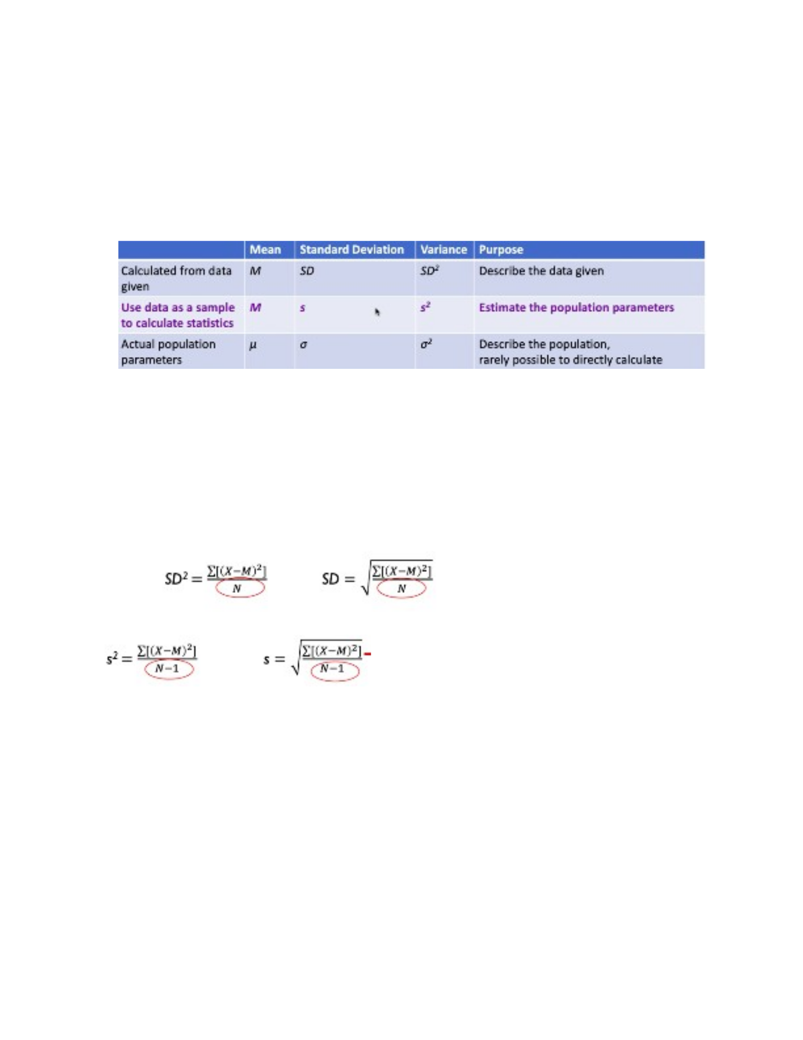
- Actual variance (SD^2) and standard deviation (SD) for the data
-
- Use data as a sample to estimate population variance (s^2) and standard deviation (s)
- By changing N to N-1, estimated population variance and standard deviation both
become larger than those describing the data set itself
Why We Care
- Goal of research is to figure out the population, but population cannot be measured
directly, thus we need to use sample to estimate population parameters
- When we analyze data to perform hypothesis testing, the hypothesis is always formulated
about the population, not the sample
oEstimate population mean and variance (standard deviation) in the process of
analysis
Variance and Standard Deviation Explained

Module 2
Normal Distribution and Z-Score
When is a Frequency Distribution Normal?
- Many phenomena, including human traits and behavior, naturally form a symmetrical
bell curve when the frequency distribution is plotted
- Commonly used statistical analyses are created with the assumption that the population
distribution is normal or near normal
- Frequency distribution: tally how many data points occur in each score range
- Normal distribution: symmetrical shape with a specific slope on either side of the central
peak
- How do we know if a distribution is normal?
oNormal curve can be drawn over a histogram to see if the distribution might be
close to normal
oA normality test can pe performed to show if a frequency distribution is
significantly different from a normal curve or not
Special Property #1: All normal distributions are alike
- Standard deviation: average distance from a data point to the mean
- If we used the SD as the measuring unit for distances between values in a distribution, it
will always come out like this, regardless of what the variable is
Special Property #2: Proportions are Known
- Think of whole normal curve as the whole population of data points, and it is possible to
mathematically figure out the proportion of any region within that distribution
o34% of cases fall between the mean (central point) and 1 standard deviation above
the mean

o
The Meaning of Z Score
- All normal distributions have the same properties (below left) and a data point’s location
in the distribution can be expressed in terms of how many standard deviations above or
below the mean
- Convert each data point into a number that indicates its location in the distribution Z =
(score – mean)/standard deviation
Use Z-Score to Location a Number in a Normal Distribution
- To calculate the Z-score for a raw score (and convert the original distribution into a Z
distribution), need to know mean and standard deviation of the original distribution
Sampling and Probability
- Probability needs to be expressed in the decimal format, not fraction or percentage

Determine p Based on Distribution Proportions
- When a sample is drawn from a very large pool (population), do not know the exact
frequencies of all possible data values; can’t calculate p that way
- If the distribution of the population is normal, we can figure out the proportions of the
different sections of the distribution and use those to calculate p for a score range
oConvert drawn score cutoff (GPA of 3.6, want the p for GPAs > 3.6) into Z score
based on population mean and standard deviation)
oPlace the Z score on the standard Z distribution and find out the proportion (%)
above that cutoff point
oTurn the proportion (%) into p
- Turning cutoff score into Z score: Z = (X-mean)/SD
Determining Population Characteristics Based on Probability of Drawing a Certain Sample
What does Probability Tell Us about Population?
- Assumption based on probability theory
oIf we only draw one random sample, (middle red circle part of the curve where
most cases are located) expect to get the most likely outcome
oIf we only draw one random sample, get something from the tail ends (outside of
red circle), serious doubt that the sample came from this distribution
Basis Logic of Inferential statistics
- If our sample has a high probability of coming from population A, then it probably came
from population A
- If our sample has a very low probability of coming from population A, probably did not
come from population A where did it come from?
oSample likely came from a population where the sample is in the center of the
distribution where most scores are
oPopulation probably look quite a bit different from population A
oCannot verify the exact population parameters because there are many
possibilities
Inferential Stats Do Not Reveal the Truth
- Collect sample data to represent the population when we can’t collect data directly from
whole population of interest
- Sample is like the population but not exact same, every time a sample is drawn, it would
be slightly different
- Relationship between sample and its population is probabilistic in nature
- Inference we make about population only provides probabilities of a certain phenomenon,
rather than proving it
Logic of Hypothesis Testing
How to Draw a Sample for Inferential Statistics
- To make a valid inference, the sample should be a good representation of the population
- Probability theory: randomly draw sample should have more of the scores that are
abundant in the population and fewer of the scores that are rare in the population

oSample mean should be close to population mean and sample looks like the
population distribution
- Larger the sample, the more likely it is a good representative of the population
How to Make an Inference from the Sample?
- Reason for drawing a sample is to find out about the population, so we do not know
exactly what the population looks like by examining our sample
- Probability theory: figure out the probability of our sample coming from a particular
population
- Set up research question/hypothesis in a way that we can test the sample against one
particular (known) population
- Inference (direct): if the p is below our criterion, we conclude that the sample did not
come from the comparison population
- Inference (indirect): if the sample did not come from the comparison population, it
probably came from some other population that is quite different from the comparison
population
oCannot pinpoint exactly what that population is like
Use Inferential Stats to Test a Hypothesis
- Research hypothesis formulated about target population, not just the sample
- Data analysis can only be performed on the sample data, so inferential stats are used to
examine the population from which the sample has been drawn
- Because sample is not the exact replica of the population, the inferences made about the
population are expressed in terms of probability rather than certainty of truth
Testing Null Hypothesis
- Null hypothesis: taking the new antiviral drug does not shorten the duration of the flu
- Hypothesis test is testing the null to find out: what is the probability of the sample
coming from the general population
- If the probability is low enough, it’s unlikely the samples came from the comparison
population, so the null hypothesis is rejected
oI infer that the population from which the sample has been drawn (taking the
drug) is significantly different from the comparison population (not taking the
drug)
- If the probability is not low enough, conclude that the sample likely comes from the
comparison population and cannot reject the null hypothesis
oI can infer that the population from which the sample has been drawn (taking the
drug) is not different from the comparison population (not taking the drug)

Why Test Null Instead of Research Hypothesis
- Rely on probabilistic relationship between sample and population, can only be calculated
with the sample data and a known population distribution (where mean and SD can be
estimated or known)
- NULL means DV (flu duration) does not depend on IV (treatment status), which means
the sample data (with drug) likely come from the general population distribution (without
drug)
Research Question to Hypothesis
- RQ: does the new antiviral drug shorten the duration of the flu (for anyone taking it?)
- Alternative hypothesis: taking the new antiviral drug significantly shortens the duration
of the flu, compared to not taking the drug
- Null hypothesis: taking the new antiviral drug does not significantly shorten the duration
of the flu, compared to not taking the drug
Interpreting Hypothesis Testing Result
- Alpha level is criterion
- Alpha level = .05
- Calculation on the sample: p = .16
- Hypothesis testing decision: probability of the null hypothesis being true (.16) is higher
than the criterion (.05), so we fail to reject the null hypothesis
- Answer to research question: taking the new antiviral drug does not significantly shorten
the duration of the flu
Uncertainty of Hypothesis Testing
- Type 1 error: rejecting the null when it’s actually true
oFalse positives
oProbability of alpha correlated to the level of confidence that you set
- Type II error: failing to reject the null hypothesis when it’s actually false
Module 3
Hypothesis Testing with One Sample
A Special Normal Distribution
Normal Distribution has Predictable Properties

- Think of whole normal curve (distribution) as the whole population of data points, and
it’s possible to mathematically figure out the proportion of any region within that
distribution
- Any data point can be located on the distribution using standard deviation as the
measuring unit, so data from different populations can be compared
- Properties of a normal distribution allows us to perform may statistical analysis for
hypothesis testing (inferential statistics)
Tendency to Become “Normal” (Central Limit Theorem)
- Special normal distribution can be created out of any population distribution regardless of
whether that original distribution is normal or not
- If many random samples are drawn from original population and we calculate a mean
from each sample, we will have a population of sample means
oDistribution will always be close to normal
Sample Size Matters
- Distribution of means contains the means of samples of the same size
- When each sample contains many scores, the distribution of means will get even closer to
a normal distribution
- Range is smaller in distribution of means compared to original distribution of scores
Meaning of Distribution of Means
- Sample is drawn to estimate population; sample mean is estimate of population mean
based on probability principle
oEach time a sample is drawn, the mean will be slightly different; some are closer
to real populations mean than others
oSample means are not perfect estimates of the population mean so there is
measurement error
Standard deviation is also called standard error (SE or standard error of the
mean)
- Larger sample is a better representation of the population based on the probability
principle, which means that those sample means are more accurate estimates of the
population mean
oDistribution of means based on a larger sample size has a smaller standard error
Purpose of Creating the Distribution of Means
- Distribution of means is also called sampling distribution
- In hypothesis testing, we calculate the probability of our sample coming from a known
comparison distribution
oIf probability is low enough, we reject null and conclude that sample likely
represents a distribution that is significantly different from the comparison
distribution
- To calculate probability of a sample coming from a specific distribution, must locate
sample on the distribution and find out if it falls into the critical region (extreme tail
region)
- If sample is single score, compare it to a distribution of scores
- If sample is multiple scores, use sample mean as representative values and compare it to a
distribution of sample means

oWhen hypothesis testing is done in real research studies, sample always consists
of multiple data points, so we convert the distribution of scores to a distribution of
means for comparison
oSince distribution of means is always close to a normal distribution, that makes it
possible for statistical analysis to work
One-Sample Hypothesis Test
One-Sample Hypothesis Test Result: One-Tailed
- H1: Alternative Hypothesis: mean of population A is significantly lower than mean of
population B (meanA < mean B)
- H0: null hypothesis: mean of population A is not significantly lower than the mean of
population B (meanA >or= meanB)
- P: probability of drawing a value at least as low as Ma from sampling distribution of
population B
- Alpha: cutoff for a probability to be considered low enough
- P>alpha: probability of null hypothesis being true is not low enough to reject the null
hypothesis
One-Tailed Hypothesis Test Result Based on Alpha Level
- H1: Alternative Hypothesis: mean of population A is significantly lower than mean of
population B (meanA < mean B)
- H0: null hypothesis: mean of population A is not significantly lower than the mean of
population B (meanA >or= meanB)
- P: probability of drawing a value at least as low as Ma from sampling distribution of
population B
- Alpha: cutoff for a probability to be considered low enough
- Because P < Alpha: probability of null hypothesis being true is low enough to reject the
null hypothesis
Two-Tailed Hypothesis Test Result Based on Alpha Level
- H1: Alternative Hypothesis: mean of population A is significantly different from mean of
population B (meanA does not = meanB)
- H0: Null Hypothesis: mean of population A is not significantly different from the mean
of Population B (meanA = mean B)
- P: probability of drawing a value at least as extreme as Ma on either side from sampling
distribution B
- Alpha: cutoff for total probability (from both sides) to be considered low enough
- P>A: probability of null hypothesis being true is not low enough to reject null
How Much is Known About the Comparison Distribution?
Two Methods of One-Sample Test
- Bottom line: find our probability (p) of null hypothesis being true and compare p against
alpha to determine if the null hypothesis can be rejected

- Direct method with SPSS (t test only, not Z test)
oSample mean t statistic p compare p against alpha
- Indirect method with reference table (both t and Z tests)
oAlpha proportion critical t or Z value using the reference table
oSample mean t or Z statistic compare statistic against critical value
Interpret Z-Test, T-Test, and Hypotheses
Z Table
The Concept of Z Distribution
- If the data points of a variable are normally distributed, it can be transformed into a Z
distribution by calculating the Z score for each raw score, using Z = (X-mean)/standard
deviation
- Z score indicates how many standard deviations are between the score and the mean
- Proportions of data points can be calculated between Z scores
The Purpose of Z Table
- Major proportions marked by the major Z scores are commonly known
-
- Z table provides proportions corresponding to a wide range of possible Z scores
What is in a Z Table?
- For each Z score, two proportions are provided in the form of percentage
- Z table provides proportions for Z scores ranging from 0 to 4.50
oNegative Z scores have mirror images of the same proportions because the normal
distribution is symmetrical

Perform a Z Test
Two Methods of One-Sample Test
- Find out probability (p) of null hypothesis being true and compared p against alpha to
determine if the null can be rejected
Scenario for a Z Test
- Only one sample (one group of data points) representing an unknown target population
- Population mean is given for a known population that is hypothesized to be different
from the target population
- Population standard deviation is also given known, so this comparison distribution can be
converted to Z distribution
oIf standard deviation is unknown, then a one-sample t test should be performed
Formulating Hypotheses
General Principles for Formulating Hypotheses (Z test and t tests)
- Hypotheses are about populations, not samples (use symbols for population)
- Hypotheses are about the whole population, not just the means
- It’s common to include the wording of significant
- Both populations should be mentioned in some way; DV must be present
- Can focus on a significant difference in any direction (non-directional) or focus on a
significant difference in a specific direction (directional)
oNon-directional: is there a significant difference between population 1 and
population 2 in terms of DV? Are population 1 and population 2 significantly
different in terms of DV?
oDirectional: is population 1 significantly higher (or lower) than population 2 in
terms of DV?
- Alternative and null must collectively cover all possible relationships between variables;
null must include “no difference” situation
- Always different ways to state same hypothesis
Practical Guide to Formulate Hypotheses
- Formulate alternative hypothesis first
oTurn the research question into a statement and use it as the alternative hypothesis
oIf research question is directional, we can either formulate a directional
hypothesis accordingly or use a non-directional version and then find out
direction of the difference after data analysis
- Formulate null hypothesis to catch the other possible outcomes

oAdd the “not” wording into the alternative hypothesis to make it the null
oWorks for both directional and non-directional hypotheses
Things to Remember
- Having a directional hypothesis does not require a one-tailed hypothesis to be performed
oPerform two-tailed test to catch any difference in either direction
oIf test is significant, examine the means to figure out direction of effect
- Make sure alternative hypothesis and null hypothesis match up in wording and symbol
notations, cover all possibilities
oIf alternative is directional, so is null
Significance and Effect Size
What does Significance Mean?
- Significant: when the test result crosses a threshold
- Hypothesis test result is the p of the null hypothesis being true
- When p is lower than the criterion (alpha level), the test is significant, and we can reject
the null hypothesis
What can Influence the Significance Result?
- Criterion (alpha level) is arbitrary, determined by the researcher
- Location of the sample mean is affected by sample size: when N is larger, SM is smaller,
test statistic is larger (more extreme)
What Doesn’t Significance Result Tell Us?
- Hypothesis test is significant in all three cases because the target population mean falls
into critical region of the comparison population
oNull hypothesis is rejected
oMean 1 and mean 2 are significantly different
- Actual difference varies across the three scenarios
- Need to know size of difference effect size
Effect Size Matters Even When Test is Not Significant
- First test is significant while the second test is not (still very similar in size)
Two Facets of Hypothesis Test Result
- Significance: is there an effect (difference) that’s statistically significant?
- Effect size: how big is the effect (difference)?
- Report p vales and effect sizes for both significant and non-significant statistical test
results
Effect Size for Comparison of Two Population Means
- Raw effect size: distance between the two means
oCan’t directly compare from different studies
- Standardized effect size: Cohen’s D: distance between two means in terms of standard
deviation, like the standardization concept of Z score
Module 4
Two-Samples Hypothesis Testing
When Two-Samples are Linked
- Repeated measures from each participant
oIs blood pressure significantly lower after taking a new hypertension drug,
compared to blood pressure before the treatment?

oDoes memory score change significantly from age 50 to age 70?
oIs there a significant difference in cognitive function between sleeping 5 hours
and sleeping 7 hours in the previous night?
- Measurements from different participants are linked
oDo twins adopted into different families have significantly different IQ scores?
oDo men make significantly more money than the women in the same household?
- When the two sets of data points are linked one-to-one, a difference score can be
calculated for each participant
- One sample of difference scores
- One sample t test: if p < alpha, Mdiff is unlikely to be 0, reject H0
When the Two Samples are Independent
- Two sets of data points collected from two different groups on the same variable
oAre American pet cats significantly heavier than Japanese pet cats?
oIs there a significant difference in COVID-19 infection rate between cities with a
mask-wearing law and cities without?
- Can be studied within-subjects or between-subjects
- No way to calculate individual “difference” scores, sometimes the groups don’t even
have the same sample size
- Calculate “mean difference” used Ma-Mb; use it for test statistic
- Compare to a distribution of mean differences from all possible samples
- If p < alpha, [Ma-Mb] is unlikely to be 0, reject H0
Within-Subjects vs. Between-Subjects Designs
Between-subjects Design
- Two levels of the IV are assigned to different subjects between-subjects
- Each subject only goes through one condition, either A or B
- Two groups of memory scores from two groups of different subjects are compared
oContrast between A and B comes from comparing between different subjects
Within-subjects Design
- Two levels of the IV are assigned to the same subjects within-subjects
- Each subject goes through both conditions, A and B
- Two groups of memory scores are compared but they come from the same subjects
oContrast between A and B comes from comparing scores within each subject
When should we Consider Using a Within-Subjects Design?
- When people naturally vary a lot on the dependent variable
oAny two groups means may look different due to natural variations, rather than
due to the different levels of the IV (factor)
Neural activities, score on a difficult memory test
- When the levels in the IV (factor) can only be meaningfully compared within the same
person
oSome IVs (factors) are within-subjects in nature
Before and after a treatment, trend over time (different time points)
Benefits of Using a Within-Subjects Design
- Some IVs (factors) are only meaningful with a within-subjects design
- Group comparison is better defined without influence from individual differences,
leading to more power in detecting a true effect
Challenges of Using a Within-Subjects Design

- Q: does memory performance differ between two encoding conditions?
- Would need two different sets of stimuli in the two conditions so subjects don’t see the
same set twice
- Need to counter-balance the order of condition A and condition B to control potential
“order-effect”
- Need to check for “practice effect” because each condition may produce different
memory performance depending on whether it’s first or second condition
- Impossible to do a surprise memory test because surprise element disappears after
experiencing one condition
- Time commitment is greater, may be harder to recruit subjects
Statistical Tests for Between and Within-Subjects Designs
Module 5
One-Way Between-Groups ANOVA
Logic of ANOVA
Concept of Variance in Group Connections
- Within each group, scores vary naturally because multiple measurements on a variable
are always slightly different
oWithin-group variance (error variance)
- Between different groups, scores also vary because the groups differ in some way (IV);
differences indicate the distances among the groups
oBetween-group variance
- When the average between-group variance is about the same as the average within-group
variance, then the groups are basically one big population and not different from one
another
- When the average between-groups variance is much larger than the average within-group
variance, then the groups are significantly different from one another, possibly coming
from different populations
How to Compare Variancewithin and Variancebetween
- Ratio to show relative sizes: F = MSbetween/MSwithin
- F>1 when MSbetween is many times larger than MSwithin
oGroups differ from one another more than the error variance (how much the
scores naturally vary within each group)
- F=1 when MSbetween is about the same as MSwithin
oGroups are not different and they could have come from the same population
Hypothesis Testing with One-Way ANOVA

Calculating Within-Group Variance
S2Within = weighted average (weighted by the different sample sizes)
- Each sample is used to estimate population variance as usual
- Assume all populations have the same variances, take the estimates from samples and
calculate the weighted average variance as the variance for all groups
Calculating Between-Group Variance S2between
- Sample (group) means become the data points in a sample, which is then used to estimate
the variance in the population of means
Manual Calculation
- SStotal = SSwithin + SSbetween
- Critical F value is obtained from the F table using DFwithin, DFbetween, and alpha
- Even if SPSS is used to compute F statistic, effect size n^2 requires manual calculation
using SPSS output
on^2 = SSbetween/SStotal (proportion of total SS that is accounted for by the
between-group SS)
Reporting F test Result in SPSS
- Format of reporting F statistic result: F (DFbetween, DFwithin) = ___, p = ___, n^2 =
___
-
-
Post Hoc Analysis
- Compares each pair of groups and see where the significant differences are

- Similar to t test but computed in a way that does not increase the likelihood of
committing a type 1 error
- Only conducted when initial ANOVA F test is significant (p < alpha) and the null
hypothesis is rejected
- Exception is when researched plans the pair-wise comparisons (with t tests) in advance,
based on existing literature
Module 6
The Concept of Correlation
Basic Concept of Correlation
- Correlation: mathematical relationship between two sets of numbers from two variables;
when two variables are involved, it’s called bivariate correlation
- Two sets of numbers have to be linked in some way or come from the same origin
(person or entity)
- Focus on scale (interval or ratio scale) variables, with the assumption that the variables
are normally distributed
How to Quantify a Linear Correlation
- Want to know if score positions in one distribution and the corresponding score positions
in the other distribution vary in any systematic way
- Two linked variables, A and B, then there are three possibilities for the linked data points
oWhen A is high, B is high and when A is low, B is low
oWhen A is high, B is low and when A is low, B is high
oWhen A is high, nobody knows if B would be high or low
- Talking about position in a distribution, use Z score to represent position of every score
Quick Review of Z Distribution
- Z score is calculated to represent the position of a data point
o(X-Mean)/SD = Z
- If data point is higher than mean, it will have positive Z score
oZ represents position of the data point as “how many standard deviations above
the mean”
- If a data point is lower than the mean, it will have a negative Z score
oZ represents the position of the data point as “how many standard deviations
below the mean”
- When the data point is the mean, the Z score is zero
Computation of Correlation Coefficient ( r )
- Convert each score on each variable into a Z score to indicate the location of the score as
high or low in the distribution
- Multiple each pair of Z scores to indicate the combined position of the pair
- Sum all results and divide it by sample size to get the average relationship
Direction of the Correlation

Strength of Correlation
- R can only range from -1 to 1
- 1= perfect positive correlation (A and B go in same direction)
- -1 = perfect negative correlation (A and B go in opposite direction)
- 0 = no correlation
Interpreting the r Statistic
- Scatter plots with stronger r statistics show a narrower band containing the data points;
the data points fit the line more closely, with less deviation from the line
- Generally, go with Cohen’s guidelines, applicable to both positive and negative
correlations
o0.1 or lower = no correlation
o0.1 to 0.3 = weak
o0.3 to 0.5 = moderate
o0.5 or higher = strong
Meaning of Correlation (r^2)
- Correlation coefficient, r, can tell us strength and direction of a correlation between two
variables
- Mathematically, r^2 indicates how much of the fluctuations in Y can be predicted or
accounted for by the fluctuations in X (or vice versa)
- R^2 represents proportion of variance shared between two variables
Outliers are Liars
- Assumptions for calculating Pearson’s r
oBoth variables are scale variables (interval or ratio variables)
oBoth variables are normally distributed
oThere is a linear relationship (use scatter plot)
oNo bivariate outliers
Correlation does not Equal Causality
- Mathematical relationship between X and Y implies no causal relationship
- Possibilities of the real relationship behind a correlation include
oX causes Y, X causes Z which causes Y
oY causes X, Y causes Z which causes X
oZ causes X and Y
From Correlation to Prediction
What is a Linear Relationship?

- Relationship between variables can be explained with a line
- Observations
oX=1 Y=2
oX=2 Y=4
oX=3 Y=6
- The relationship is represented as Y=2x + 0 (Y is the slope)
Components of a Linear Relationship
Why do we Represent the Relationship in a Math Function?
- If we know there is a linear relationship between X and Y AND we observe that when
x=1, y=3 and when x=4, y=7
oPlot relationship as Y = 1X + 3
Linear Relationships in Research
- Data points never actually form a straight line
- Each point on the scatter plot represents a linked pair of scores
- If the dots roughly form a thick but straight line, there is a suggestion of a linear
relationship between X and Y scores in the sample
- If the sample is a good representative of the population, it can be hypothesized that the
linear relationship exists beyond the sample
Linear Relationship Between 2 Variables: Bivariate Correlation
- Identify a straight line that captures the most data points – yielding the LEAST total
deviation of the data points from the line
- Specify how accurate the predictions from the linear function can be
oR = 1 perfect positive correlation
oR = 0 no correlation at all
oR = -1 perfect negative correlation
From Bivariate Correlation to Bivariate Regression
- Linear relationship between 2 variables is bi-directional by nature
- r^2 indicates proportion of variance I one variable that can be explained by variance in
other variable (shared variance)
- Regression equation is one way to represent linear relationship (correlation) where one
variable is designated as the outcome variable (Y) to be estimated by the predictor
variable (X) through the question
oDesignation of predictor and outcome variables should be based on a theory or
existing research findings

oY= bX + a (Y is estimated Y score based on the known X score associated with
the Y)
How Far can we go with a Linear Relationship?
- When a hypothesis test on regression is significant, Y can be predicted or estimated by
knowing its associated X
- Prediction in correlational analysis means that there is a purely mathematical relationship
between X and Y such that we can plug X into the linear function (formula) and calculate
an estimated Y
- Prediction does not imply causal relationship
- Prediction does not imply a a temporal sequences of Y following X or X following Y

