



Lab 3 - Seth Gibson - MAT 275 Lab
Introduction to Numerical Methods for Solving ODEs
Contents
■ Exercise 1
■ Exercise 2
■ Exercise 3
■ Exercise 4
■ Exercise 5
Exercise 1
Part (a)
% Define ODE function f for ODE dy/dt
f = @ (t,y) (3*y);
f
(t,y) 3y.
% Define vector t of time-values over the interval [0,0.5] to compute
% analytical solution vector.
t = linspace(0,0.5,100);
% Create vector of analytical solution values at corresponding t values.
y = 2*exp(3*t);
% Solve IVP numerically using forward Euler's method with 5 timesteps.
[t5,y5] = euler(f, [0,0.5],2,5);
y5 (end) ;
% Solve IVP numerically using forward Euler's method with 50 timesteps.
[t50,y50] euler(f, [0,0.5],2,50);
y50 (end);
% Solve IVP numerically using forward Euler's method with 500 timesteps.
[t500,y500] = euler(f, [0,0.5] ,2,500);
y500 (end);
% Solve IVP numerically using forward Euler's method with 5000 timesteps.
[t5000,y5000] = euler(f, [0,0.5],2,5000);
y5000 (end);
% In the following steps, we define error as analytical (solution value
% - numerical solution value).
% Compute numerical solution error at t=0.5 for forward Euler with 5
% timesteps.
es = y(end) -yS(end);
% Compute numerical solution error at t=0.5 for forward Euler with 50
% timesteps.
e50 = y(end) -yS0(end);
i
_
:
2
o
:
:
o £
©”
:
£
2
|
£
=
s
|
=
_
-
os
c
a
DS
:
2
6
°
:
uw
©
8
:
oa
©
£2
2
o
e
Ps
£
Oo
”
:
%
e
Oo
°
:
tid
E
2
ey
3s
:
fe
a
F
a
a
o
:
ee
wy
S
c=
:
a
oo
3
2
S
L
5%
|
nL
ot
rs
ct
Os
o
|
os,
“eet
os
3
2S
ie
nee
c
>
a
‘a
wn
ao
rn
|
g
ag
Bo
¢E
|
ee
is
oe
G
”
c
o
_
a
ba
oo
x
:
cee
A
eote
ne
we
CON
GEN
Na,
c
S
o
CC
i
i
me
he
Be
io
.
.S
s55
Ss
o
5
2
"8
ss
a
ees
pas
ues
cena
bese
cbnee
bees
-
oO
a
ne
‘:
z
Ber
LG
Pc
£5
2
vs
éi3
Oo
a
3
Q
ee
fb
5
2
c
3
a
.
.
Bp
PB
ee
|
¢5
co
:
.
those
:
va
:
;
>
w
oO
2
i
&
ae
gor
$
sa
a
i
‘
—
:
é
s
é
ie
”
t
i‘
Se
o
Ss
a
:
ee
M
Y
eo
o#
i
o£
a
a
Shot
in
fet
bay
WSS
SESS
ESSE
4i
Oo oO
o
:
Y
ae
=
Oo
oD
i
#5
3
oe
®a
2
ak
o
“
.
:
eo
21
>2
of
:
Ce
;
a
e
‘
:
Po
Oy
bo
:i
<&
:
ean
Q
:
oo
|.
ee
ee
:
ge
go
|
BS
f
ie
3
a
if
:
oe
;
:
aes
ony
;
i
_
wo
_
GES
i
43
ad
:
%
;
Coot
AGE
a
5
2
®
=
|
&
ys
wo
a
j
ey
H
EE
gee
feat
;
‘
=
O
oO
:
MEER
a
:
Sa
eee
~o
2
ee
4
4
e
Sor
eee
a2
Eo
,
Looe
GS
ad
i
Ya
“
pot
''
Cc
Oo
5
£
:
eo
;
;
i
=
2g
:
3
a
i
7
oe
©
O
:
re
:
Z
:
Q
oD
eas
“
:
Zi
Be
Oo
2
cc
e
_
S
G
Po
:i
ec
3
8
:
“sw
ee
iw
peed
i
S
2
Boy
oi
ow
@
‘he
Peay
hoot
A
':
a
_
w
D
oe
BE
o
=
4
os
=
H
ee
ai
i'
=>
_.
Ce
:
N
ee
5
fb
Eg
8
2
4
Pea
eee
:!
sc
6CU§
:
A
Boe
eB
-
i
PBF
ip
a2
<6
:
Ne
a
q
=
o
2Q
0
hd
boa
bts
oe
Oo
=
os
eos
6
§
6
6
-
s
Pe
ge
72
Go
66S
,
opt
n
Se
6
SE
:
Ce
bei
a
!:
£5
%&€
|
Vs
|
o
iD
°
-
8
;
2
Oo
=
oO
pH
Oo
wn
hese
egy
net
'
pdt
,
a
Oo
S
®
,
28
Ww)
>
es
iO
i
fot
!
o
©
a0
,
=~
a
i
&
oO
oe
:
'
i
N
o
os
»
3
2%
6h
‘~
eS
88
fo
2.
:
aS
85
HN
5
a
:
©
Py
oe
2.2
XD
6
522
CG
6-6
B65
20
S
!
oo
WO
eq
mo
0
©
O
ey
oO
eo
eo
OQ
@
Ug
3
&
Be
—
iy
~~
*
a
Pence
eee
tenes
H
@
o
2
Ss
o.
a
B
g
i,
oO
oe
ie
,
|
o
—
rh
a
oS
wn
ae
D
;i
mf
-
5
-
w
2:
_~
oO
on
;
fl
ie
aD
yl
77
oo
|
$3
68
oF
2
ue
‘dt
ee
_
a
ar
aQ
2
A
S
:
Q
5
i
wa
a
~"
tc
®o©
c
c
@
:
x
reves
si)
joan
Oo
S
LS
a
|
©
14
©
Po
o
N
oe
©
x
6
“5
~
:
Po
sree
cee
cee
en
ane
i
IN
x
a
OQ
L-)
Ley
wn
pee
e)
ver
ose
a
3
a
tT
wn
@
Bee
ot
sy
ce
Peas
Mee
“
@
ler
oamnn
ere
i
~=~=—hC—ChCClC
rr
i
aqY
=
-3*Y;
%
dy
=
-3*y;
this
is
the
ODE
quiver
(T,Y,daT,dY)
%
draw
arrows
(t,y)->(ttdt,
ttdy)
axis
tight
%
adjust
look
hold
on
ey
a
20
ee
whe
ole ole
we
ob
ed
oo
a
a
{Bb
+
+a
oH
a
+
ttt
ts
td
dt
a
4
OAL
we
oe
Oa
a
od
Oa
a
a
Oo
Oke
a
+
--
A
+t
2d
tb
te
Ae
Ee Da
db
or
I
Uv
UD
OL
WP
aA
ow
a a
aA
ke
ke
RD
ke
A
dR
de
a
de
A
4
ea
a
eK
eK
a
a
a
OO
BP
Or
---
-
-
sii
iii
iii
ii ii
iii.
Po
ORR
POT
Re
J
a
as
irr
Soi
rar
hs
ia!
hoa
hia
Soca
Sein
eel
Relies
Rs
Seas
DeasSea
Be
To
Pe
AB Pp
te
ttt
LTPP
PPP Pee
PPP
PPP
Pt
pg
Ce
cc
te
oh op
ph
of
pp
ee
pe
ope
of
pp
ep op
om
0
0.5
1
1.5
2
2.5
a
3.5
4
45
Part
(b)
figure
(1)
t
=
0:.3:5;7
y
=
-20:2:25
;
%
define
grid
of
values
in
t
and
y
direction
[T,Y]=meshgrid(t,y);
%
creates
2d
matrices
of
points
in
the
ty-plane
dT =
ones(size(T));
%
dt=1
for
all
points
dy
=
-3*Y;
%
dy
=
-3*y;
this
is
the
ODE
quiver
(T,Y,daT,dY)
%
draw
arrows
(t,y)->(ttdt,
ttdy)
axis
tight
%
adjust
look
hold
on
%
Define
vector
t
of
time-values
over
the
interval
[0,10]
to
define
analytical
solution
vector.
t
=
linspace(0,
5,
100);
%
Create
vector
of
analytical solution
values
at
corresponding
t
values.
y=2*exp
(-3*t)
;
%$
Plot
analytical
solution
vector
with
slopefield
from
(a).
plot
(t,y,
'k'
,
'linewidth'
,2)
hold
off

pode
ef
ee
ee
a
a
20
Fy
we we
A
A
a
wp
A
ep
we
a
op ob
eb
A
whe
aL wb
ale
we
we
oe
ee
Re
+ +
+H +H
Hie
te
Hei
A
He
A
OLY
tide
ott
+
+o
+
2a +t
atta
wa +b
a
oa
A
rE
IE
Pt
BR rh
hu
rhlUl
lh
Ul
ll
oO
Wrao
a a
4A
4+ aA
+ A
4A
4 a
ae
A a
A
dk
a
ek
a
a
i
eK
a
eo
ea
ea
ea
a
BP
LY
shit
b
i
Pitti
hpi
iii.
oe
407
TT
RT
RR
RRR
RR
To
Re
Rr
Po
ASP
PoP
oP
Pp
oP oP oP
oo
oP
oo
PEP
PPP
PPP
PPP
PPP
Pp
9g
Cheetham
0
0.5
1
1.5
2
25
a
3.5
4
45
5
Part
(c)
figure
(2)
type
'euler.m'
t
=
0:.3:5;
y
=
-20:2:25
;
%&
define
grid
of
values
in
t
and
y
direction
[T,Y]=meshgrid(t,y);
%
creates
2d
matrices
of
points
in
the
ty-plane
dT =
ones(size(T));
%
dt=1
for
all
points
dY
=
-3*Y;
%
dy
=
-3*y;
this
is
the
ODE
quiver
(T,Y,daT,dY)
%
draw
arrows
(t,y)->(ttdt,
ttdy)
axis
tight
%
adjust
look
hold
on
x=linspace(0,5,100);
t=x;
y=2*exp
(-3*t)
;
plot
(t,y,'k-',
'linewidth',2)
%
Define
ODE
function.
£=@(t,y)
(-3*y);
$
Compute
numerical
solution
to
IVP
with
6
timesteps
using
forward
Euler.
[t6,
y6]=euler(f,
[0,5],2,6);
Plot
numerical
solution
with analytical solution
from
(b)
and
slopefield
from
(a)
using
circles
to
distinguish
between
the
approximated
data
de
oP
ol?
(i.e.,
the
numerical
solution
values)
and
actual
(analytical)
solution.
plot
(t6,y6,'ro-',
'linewidth',2)

hold
off;
%
end
plotting
in
this
figure
window
function
[t,y]
=
euler(f,tspan,y0,N)
m
=
length(y0);
tO
=
tspan(1);
tf
=
tspan(2);
h =
(tf-t0)/N;
%
evaluate
the
time
step size
t
=
linspace(t0,tf,N+1);
%
create
the
vector
of
t
values
y
=
zeros(m,N+1);
%
allocate
memory
for
the
output
y
y(:,1)
=
yO';
%
set
initial
condition
for
n=1:N
y(:,ntl)
=
y(:,n)
+
h*f(t(n),y(:,n));
%
implement
Euler's
method
end
3
t=
t';
y=y';
%
change
t
and
y
from
row
to
column
vectors
end
pe
pe
pe
dL
Pe
ee
pp
20
Fy
we we
LL
we
wb wb we we
we
eb ea
ee
eb
a
iGQre
+ + 4
+7444
444
848
~~
1
whe
ode
ke
a
ea
a
ae
4
Oo
a
Oo
OOo
a
OO
Wf>a
wa aA
aA
A
wa
ke
a
aA
a a
Ak
Bee
ke
a
e
a
a
eO
OF
Spon
oe
LF
IY
DS
Or
-
stoi
ie
Pi
IN~
ifs
RoR
rT
4gbr
TOR
RRR
RRR
Re
PT
o-
|
rt
a
ee
a
es
as
ee
a
es
Ds
Ceca!
Diehoi
i
Tr
oT
Te
~
oT
“VS
Pp
ht
tt
oP
PPP PPP
PP
PP
PP
PP
PP
og
KI
a
oh
ho
ot
te
oh
0
0.5
1
1.5
2
25
a
a5
4
45
5
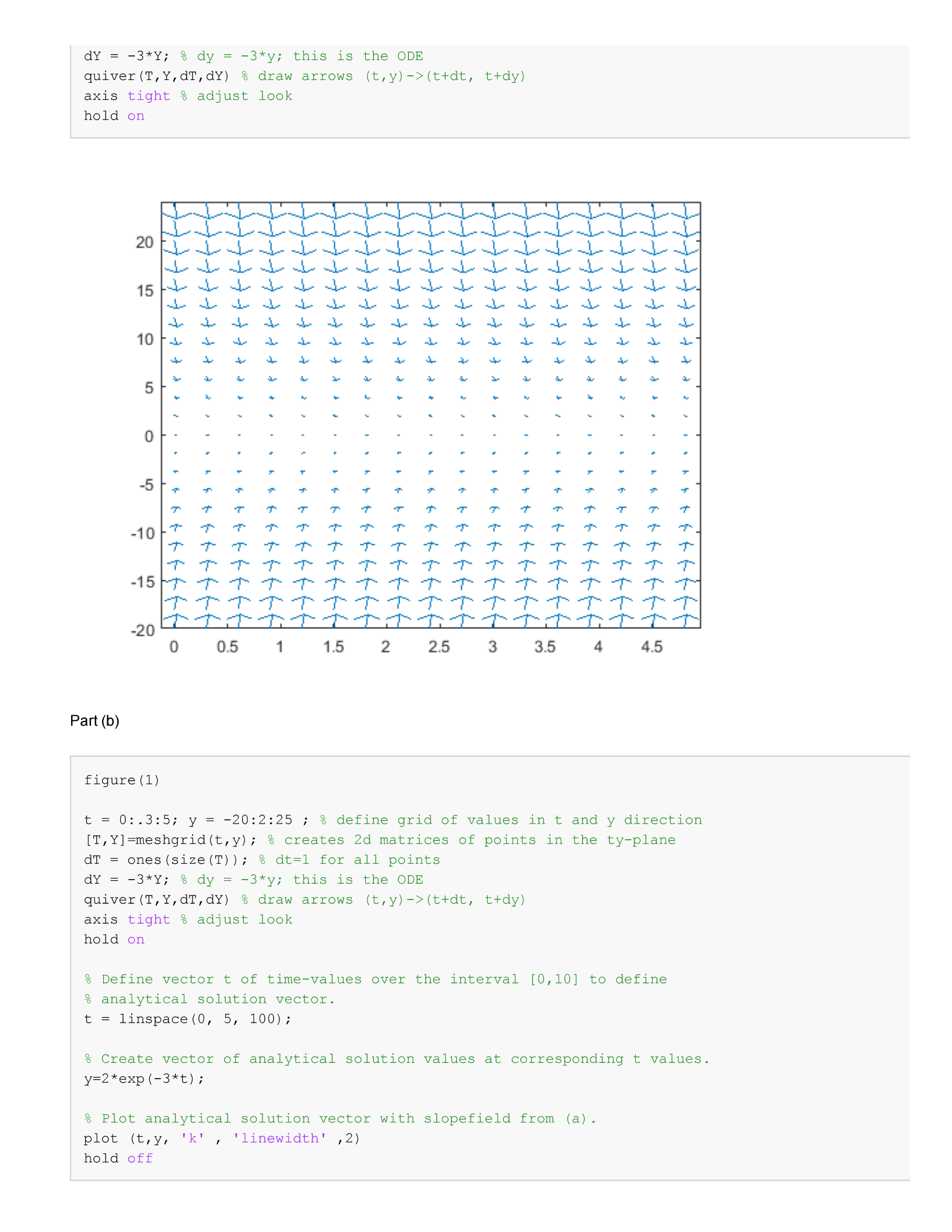
The
applied
Euler's
method
for
this
function
appears
to
be
very
inaccurate
relative
to
the
exact
solution
function.
The
approximations
follow
the
slope
direction
field
at
certain
points,
and
each
approximation
will
only
follow
the
direction
field.
Because
the
direction
field
has
a
different
slope
at
points
further
away
from
the
exact
solution,
the
applied
Euler's
approximation
will
appear
to
oscilate
and
become
more
drastic
as
t-values
become
greater.
Part
(d)
%
Define
new
grid
of
t
and
y
values
at
which
to
plot
vectors
for
slope
%
field.
figure
(3)
nfs
SS
as
Soe
on
ww
Ae
ore
ae
at
os
sy
fe
we
t
c
,
Sa
en
Pus
oo
bk
on
che
oo
we
wea
o-
re
nae
fat
nee!
oni
yee
te
det
ee
peel
Pre
‘
eee
oy
4
it
Sa
ify
ee
waa
ed
a
of
ot
ba
tt
on
ae
shee
*
fda
ot
fy
aes
oe tt
ond
;
“i
spa
oh
ve
2
is
a
*
i
ar
we
$53
ae
mS
he
od
te
*
fed
an
wheat
-s at
fe
7
is
G
npeod
ne
re
rts
ae
aay
os
ey
on
*
soak
;
ow
om
ere
ae
Ai
ty AN
4
aa
fe.
“ss
chad
4
ay
N
ree
on
os
a
int
‘
eh
ed
ea
we
.:
eS
west
bed
cae
pe
ee
tes
a
a
ea,
ass
om
an
rr
te
oa
det
&
3
12)
bo
“
,
as
mt
:
‘
s
ah
oo
i
i
La
oe
ny
ot
nant
ort
ch
ent
i]
ee
100);
N
ow
Le)
Ni
~
©
Dy
NS
ee
we
~
SON
em
Ww
Q4y
po
Paces
~
oe
Tos
<
~
4
ne
OO
SHS
Oo
_
@
-4d
oN
BH
=
a
ro
mos
Sed
oO
Oo
*
fo
N
beh
Oren
s
Oo
9
pa
DO
poor
w
GQ
DA
o
|
eal
A
rest
Wea
BES
Qo;
—
a
~
wos
3
QO
Oe
Hoo
n
=~
N
N44
wD
i
CO
eo
Gg
Pa na
Bod
as
rite
ne
PO
Sa
“4
~
my
Sho
WG
-
mo
o
rc
p
.
too
at
oO
Pb
I
Bn
=
N
io
Pore
;
QO,
s
Asad
Hi
Se
a
me
Oe
SS
at
BOAO
eA
OOK
Oo
Il
h
tO
p
a
poe
OO
Or
mG
bp
a
=
OG
er
che

0.5
f
Poe
fh
f
f
fF
PP
Pf
PP PP
PF
PD
Pre
pe
PPP
pepe
pe
d.
45
o
4
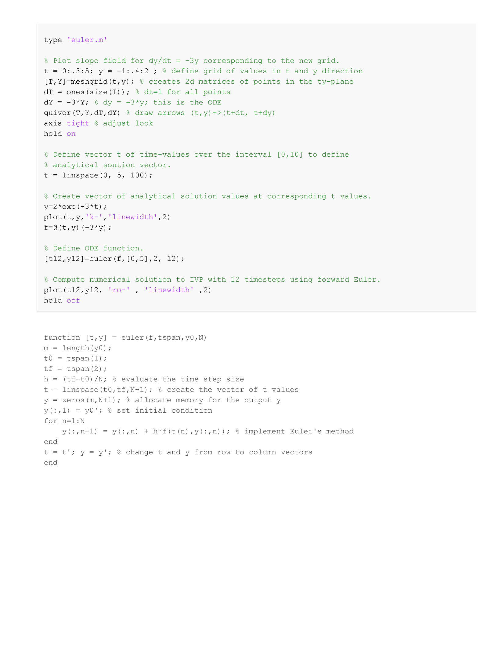
Because
the
function
decreases
so
quickly
near
the
beginning
values,
the
step
size
is
too
small
to
geometrically
appear
accurate
to
the
exact
solution,
as
the
slope
near
t=0
is
very
different
than
the
slop
at
t=0.5,
causing
the
applied
Euler's
method
to
'dive
down’
much
more
quickly
than
the
function.
The
applied
Euler's
method
oscilates
back
up
and
more
closely follows
the
exact
solution
after
t=0.5,
as
the
slope
does
not
change
drastically
with
respect
to
t.
Exercise
3
2
$
Display
contents
of
impeuler
M-file.
type
‘imeuler.m'
%
Define
ODE
function
for
dy/dt
=
f(t,y)
=
3y.
£=@(t,y)
(3*y);
oe
Compute
numerical
solution
to
IVP
with
5
timesteps
using
"improved
6
Euler."
[t5,y5] =
imeuler(f,
[0,.5],2,5);
function
[t,y]
=
imeuler(f,tspan,y0,N)
m
=
length(y0);
tO
=
tspan(1);
tf
=
tspan(2);
h =
(tf-t0)/N;
%
evaluate
the
time
step size
t
=
linspace(t0,tf,N+1);
%
create
the
vector
of
t
values
y
=
zeros(m,N+1);
%
allocate
memory
for
the
output
y
y(:,l)
=
yO';
%
set
initial
condition
for
n=1:N
fl=f(t(n),y(:,n));
>
s
Se
.
ee
‘
:
*
‘
iu
oo
:
ih
as
ib
ch
05
:
oy
bod
on
ae)
a
Pe
t
it iy ea
a
4
ip
Fe
:
ae
:
ws
4
i
2G
ao
He
:
a
io
is
ah
:
oe
;
:
os
:
2
ny
tse
wy
eas
:
ce
ae
oa
oo
aS
:
$e
aS
ep
a
:
>
tet
oe
oo
ue
un
wu
z
oi
a
wy
:
een
ene
eon
we
bi
:
ant
ae
an
om as oh
Bape
&
:
et
oo
wet
tad
os
mt
CPG
ra)
43
:
4
ced
4
eh MD
i
&
%
B
ie
5
es
wl
rt]
:
bt
ia
be
ie
po
:
oo
fe
as
c
cag
:
po
1%
S
toe
mg
:
ao
uo oh
“
oe
ce
G
&
ao
wee te
ey
:
ny
as
we
ae
‘
rd
;
oer
Set
wane
%
we
wees
a
:
oy
oh
4
ers
t
4
wo
oo
:
“pt
‘
Bl
:
ey
oS
i
:
G
ag
“
G
im
ce
u
we
:
tat
oa
no
*e
oa
Ged
the
we
ais
*
me
cana
¢
eat
*
ae
get
Pa
:
oe
:
i
a
wt
oS
ee
3
aS
uo
:
ot
sy
_~
ay
cc
:
od
bes
oe)
iy
es
ed
:
“~
Oo
ie
Cees
:
~~
oO
2p
:
OS
WZ
pet
Bo
eet
in8
:
o3
os
©
.
te
14
G
ect
ws
=~
-n
N
ot
:
So x
.
be
at
jet
:
~
it)
N
=
£3 oO
a
<S
~
..in
oi
S
;
fo)
:
La
N
—
®bod
G
se)
oO
.
.Ln
oO
Bs
:
e
ae
a
oO
:
BN
mc
.
es
re
oe
fed
SEONG
i
o
:
Choos
wo
o
ao
3
ie
~
a
ih
3
eee
3
=
wo
he
‘
~
hoe
iG
4
—~
53
be
ia
me
ba
Q
:
SS
ww)
oO
©
eos
ved
at
;
os
Oo
o
:
fet
oo
®
=
mae
Sey
chet
fee
ae
a
a
us
c
:
oO
oO
~
oo
is os
or
at
oO
oO
‘et
—
:
a
4
qy
poy
inet
wat
—~
4
G
rent
—
ey
‘S
:
rt
©
~
~~
i
Oo
~s
a
oO
<
o
iD
°
tet
:
om
pg
ee
qy
tS
efor
ro
_~
te)
GS
Io
—
ar
©
+
~~
:
_
pee
Se
cs
oO
oO
;
my
8
0
ie
8
g
S
&
3
c
:
©
CoM
4
rc
aO
G
ved
=)
wet
i
;
=
:
Q
hee
oO
3
Tee
oO
a
uw
a
A
tho ied
See
oh
Oo
:
o
bey
re
o
fio
—
uw)
Dy
3
an
3
oO
~
:
~
wo
®
3
g
i
sd
Le}
Ny
“rl
|
oO
—_
:
$e
.
£53
a
to
ae
rs
nt
&
a
SG
ee
3
u
q
iy
ll
ia
A
4
|
o
oe
20
oO
:
~
ce
=
aa
ae
|
we
=~
eed
ree
Ww
=o
:
Ne
B®
“
Sel
Bora
<
I
re
—
oO
tet
fo
oO
c
:
SN
Oe
es
&
©
as
S
&
Oo
*
Gq
eo)
NN
©
:
Koop
feeoar
pao
|]
oe
Soo
_~
Oo
S
foo
Y
geo
®D
Q
bot
Oo
OQ
Dik
ce
es Pe
@
feo
oO
G
oO
omnes
~NS
©
in
on
=
+
oo
G
¢
rt
|
pa
a)
re
2
G
wv
S
Go
OQ
10
eee
”
Ces
=
o
Ln
o
=
i
tO
2
@
ae
oe
~~
@
:
Py
Qu
Oy
om
GLO
GON
wos
—
a
ol
®
co
ad
5
~*~
:
SK
pel)
TN
a
-
pee
mt
lI
aa
Paced
ay
43
a.
—
poe
Ge
®
Ba
eee
oO
i)
lI
oO
te
“es
/;
_
oO
wo
fo
eK
oo.
oO
co)
oO
II
oO
tO
a)
os
rk
ren
t
np
ary
4
ay
4
2
¢
G
>
fn
—
BN
GEOL
ow
Ww
GEO
oO OQ
4
O
OQ
£20
3
oe
°
O
x
eee
eee
eee
pp
p
p
9
LO wn
wn wn
a)
44+
i}
>
x
oO
:
Qa
ay
oo
oa
ooo
oe
av
oh
oO
peg
eo
ey
Bee
he

Part
(b)
Because
the
step
size
decreases
by
almost
10
and
the
error
decreases
by
almost
100
in
the
last
column,
the
Improved
Euler's
method
is
of
order
h*2;
i.e.
as
the
step
size
decreases
by
a
factor
of
k,
the
error
decreases
by
a
factor
of
kA2.
Exercise
5
Part
(a)
same
as
in
Exercise
2
(see Exercise
2a)
Part
(b)
same
as
in
Exercise
2
(see Exercise
2b)
t
=
0:.3:57;
y
=
jJ=meshgrid(t
an
=
ones
(size(T
dY =
-3*Y;
&%
Sy
aod
quiver
(T,Y,dT,dY)
=
draw
arsows
(f.,yvickefhtat,
tbody
axis
Eight
§
adiust
took
hold
en
t=linspace
(0,5,100);
y=2*exp
(-3*t)
;
plot(t,y,
*8-',
'iinewidth',2)
Se
SAEs
SS
EOE
AES
SS
A
sy
eS
Ee
Se
A
Lt
a2
te
ik
BUONO
Eg
f=@
(t,
y)
(-3*y);
Py
:
x
~
foo
Sheen
~
SPY
a8
x
Ry
CONE
GAUSS
GES
USS
UES
EBA
CONSENS
ey
+
yan
Yet
~
SohERESE
g
¥
Ww
WINST
SR
eh
io
i
8
RESP
[t6,y6]
;
y
r
~
:
.
we
S
.
2
ke
m
~
™
ee
osc
Sey
See.
4
+
*
en
¥
ie
SENN,
=
VN
ERT
ON
Sy,
eae
i
eee
Rom
SEQ
AS
aS
OSES
ES,
at
Acs
toe
OEE
oS
SONGS
NERO
REDE
x

from
(a)
using
circles
to
distinguish
between
the
approximated
data
ae
0
(i.e.,
the
numerical
solution
values)
and
actual
(analytical)
solution.
plot
(t6,y6,'ro-',
'linewidth',2)
hold
off;
%
end
plotting
in
this
figure
window
function
[t,y]
=
imeuler(f,tspan,y0,N)
m
=
length(y0);
tO
=
tspan(1);
tf
=
tspan(2);
h =
(tf-t0)/N;
%
evaluate
the
time
step size
t
=
linspace(t0,tf,N+1);
%
create
the
vector
of
t
values
y
=
zeros(m,N+1);
%
allocate
memory
for
the
output
y
y(:,l)
=
yO';
%
set
initial
condition
for
n=1:N
fl=f(t(n),y(:,n));
f2=f
(t
(nt+1),y(:,n)+th*f£1);
y(:,;ntl)
=
y(:,n)
+
h/2*(£1+f£2);
%
implement
Euler's
method
end
t=
t';
y=y';
%
change
t
and
y
from
row
to
column
vectors
end
30
F
py
—_-
Ls
20
Fy
ww
oy
ww
ww
HL
—1-
—-
~-
|
-A- -Le
-e
w
d
a
t-te
whe
oO
Ot
mete
OO
wh
ke
a
Oo
a
a
ek
a
Oe
-A-
ok
Ook
wen
eo
a
a
we
ek
a
17a
oe
ea
ea
ea
ee
oe
oe
os
aa
ea
ea
-L-
a
a
ae
Or
=
re
os es
es
i:
oe
a
2
os oe
2
es oe
rs
AOR
Or
STR
TR
RT
RRR
Rt
oop
pt
ttt
SPT
20
Wo
a
ea
a
oe
()
0.5
1
1.5
2
25
3
3.5
4
45
5
Part
(d)
Define
new
grid
of
t
and
y
values
at
which
to
plot
vectors
for
slope
field.
%
%

oe
:
ee
.
‘
ot a
tt
:
ct
:
£3
:
Oe
fatde
‘
foe
oot
fer
.
Bee
ie
:
roe
ee
on
.
honey
oo
*
aeare
ves
Cee
4cnet
*
seep
eyes
i
::
peo
3
:
Pat
ws
ee
3
ae
vs
:
ot
oo
:
&
hey
ys
:
Aegon
vas
.
CE
te
:
fest
on
aoe
ery
ng
ne
©
:
wen
nore
nee
:
hers
me
on
:
cS
neat
:
CRA
:
hos
eet
:
Eee
ree
+
ae
eae
,
na
he
_
its
ie
ond
wy
:
pot
md
*
ot
ay
ae
i
:
mS
:
a
:
ao
:
oo
wy
:
on
‘
fe
:
rane
gos
7
af
job
:
vet
a
:
Ba
ba
G
:
on
a
peak
:
aerate
a
:
a
we
:
oF
a
:
fed
eal
~
:
“
Eg
©
ao
ie
_
i
Cc
seh
4d
we
i
N
:
;
%
@
&S
a
:
ag
Cs
ct
vd
4
eet
Aye
os
S
:
a
@
SR
bet
pee
N
N
:
heb
eof
Lb
pg
~
x
:
ma
td
By
”
=
Ord
foo
ad
pg
Ep
ee
“ey
:
Om
4
ee
OS
TE
pein
ao
«
:
peed
oe
ged
on
Veg
bh
OS
geo
ge
D>
ae
2
Oo
od
4
we
es
oO
ot
co
or
ood
:
Ce
ord
os
Fe
.
:
a
PRE
ES
Meg
5]
eee
ee
*
>
hs
eens
thet
co
oe
i
:
~
ee)
fe
AO
o
“rd
moo
oS
:
we
ae)
Sor
3
vt
aD
pa
=
OGG
hE
;
a
oy
ie
:
ae
°
oO
Se
Cpe
eS
aN
RS
ep
:
von,
“
Et
bes
=
eo
eee
vo
:
oo
4
oO
poe
®
ep
*
pos
:
Bay
m
s
woos
Oo
ax
m
tod
:
gp
le
ny
ae
fey
‘
.
ood
GQ“
pi
PEE
mom
I
mol
:
weet
_
na
n
sQ,
|
~~
pane
Wd
iO
oO oO
H
ay
n
Qo
~
Geom
cn
=~
G
=
es
q
te
QO,
Pa
cod
a
Q
fo
O
4
ned
oa
BOO
~
eh
g
4
=
oO
tel
wo
@
p
ee
ond
DB
eat
i
bhoK
=
won
:
Oo
x
=A
iy
tl
LroN
@
a
|
:
be
“A
EA
EA
pa
Il Il
oo
:
.
a
Ww
me
TO
oF
CAR
ge
a
qQy
cag
:
re
Md
¢
y
Smad
=

2
1.5 \ t t ( t t ( t t t t t t t t \
\ \ \ \ \ \ \ \ \ \ \ \ \ \
0.5 \ \ \ \ \ \ \ \ \ \ \ \
..,,. "- "- '.. '.. '-.. '-.. '-.. '-.. '-.
0
/ / / / / / / ,., ,., ,.. ,.. ,.. ,.. ,.. / /
-0.5 I I I I I I I I I I I I I I J I
-1
0.5 1 1.5 2 2.5 3 3.5 4 4.5 5
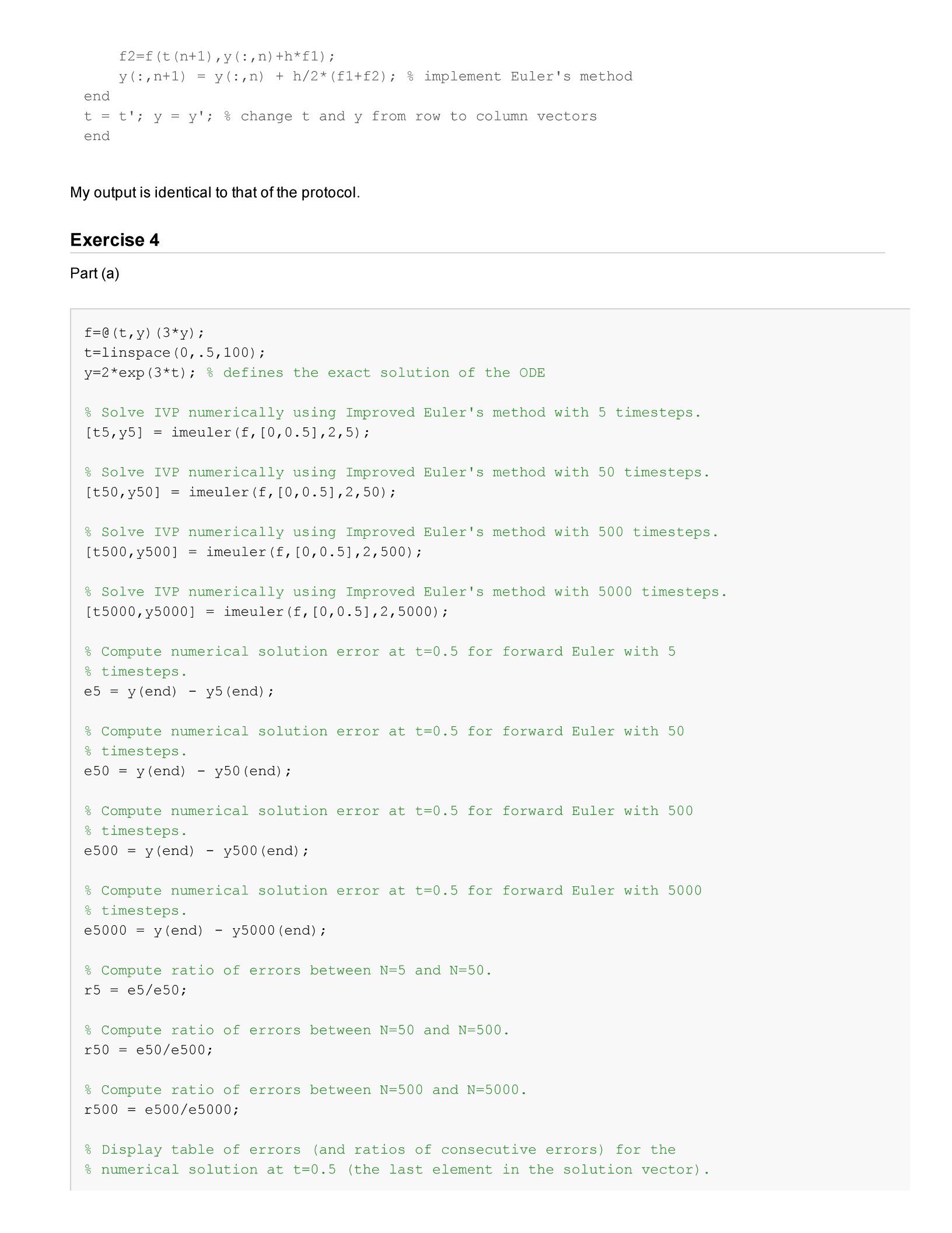
Figure 5 seems to have an applied Improve Euler's method that does not follow the field direction vectors whatsoever. I
do not understand why this is except by understanding the nature of the lmpoved Euler's method. However, because of
the average taken in the Improved Euler's method, we are able to have less 'dramatic' slopes that help the applied Euler's
method appear more geometrically accurate to the exact solutions in Figure 5 and 6.
Congratulations, you're done!

