


%% Lab 1 – FENIL PATEL - MAT 275
%% Exercise 1
% Define input variable theta as discretized row vector (i.e., array).
theta = [0, pi/9, pi/7, pi/6, 7*pi/6, 8*pi/7, 9*pi/8];
% Define radius.
r = 5;
% Define x and y in terms of theta and r.
x = r*sin(theta);
y = r*cos(theta);
% Check that x and y satisfy the equation of a circle.
r = sqrt(x.^2 + y.^2)
r =
5.0000 5.0000 5.0000 5.0000 5.0000 5.0000 5.0000
%%
% Yes, x and y satisfy the equation of a circle as we got the output r =5
for all %value of theta. The vector output was equal to the radius
defined and thus it %confirms our answer.
%% Exercise 2
% Define t-vector.
t = 3:0.15:15;
% Define y-vector.
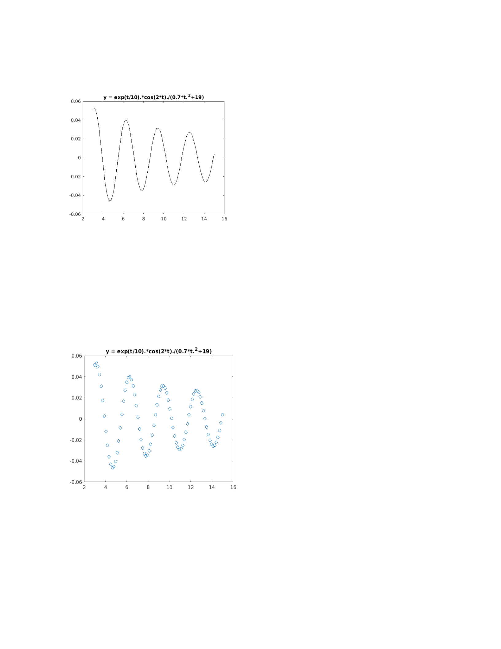
y = exp(t/10).*cos(2*t)./(0.7*t.^2+19);
%%
% Part (a)
% Plot results (should have 3 plots total).
figure;
plot(t,y,'k');
title('y = exp(t/10).*cos(2*t)./(0.7*t.^2+19)')
%%
% Part (b)
% Plot results as data points only and as data points with line.
figure; % creates a new figure window for next plot
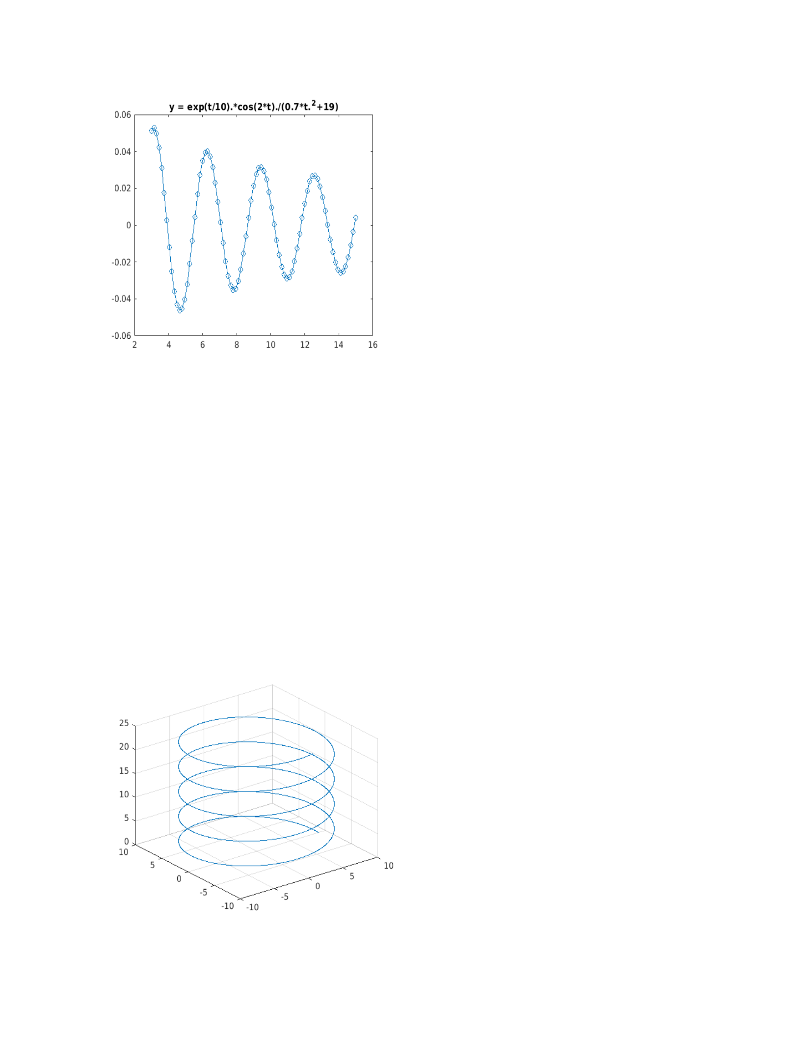
plot(t,y,'o');
title('y= exp(t/10).*cos(2*t)./(0.7*t.^2+19)');
figure; % creates another figure window
plot(t,y,'o-');
title('y= exp(t/10).*cos(2*t)./(0.7*t.^2+19)');
%% Exercise 3
% Create t-vector (choose enough elements so that plot is smooth!)
t = 0:0.001:5;
% Define x,y,z components in terms of t.
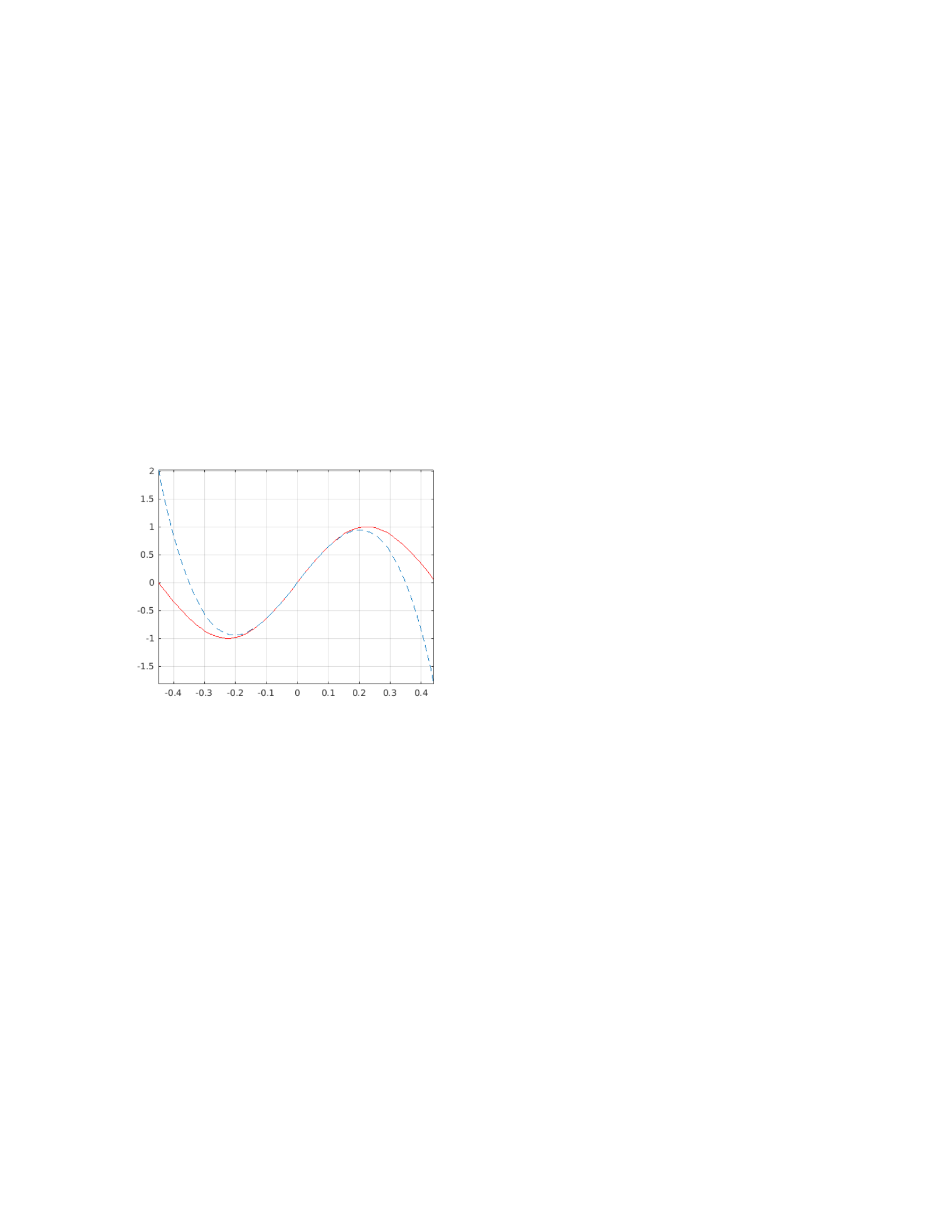
x = 9*cos(6*t); y = 9*sin(6*t); z = 5*t;
% Plot result.
figure;
plot3(x,y,z)
grid on
%% Exercise 4
% Define input variable as vector.
x = -pi/7:0.01:pi/7;
% Define y and z.
y = sin(7*x);
z = 7.*x-343.*x.^3/6;
% Plot results.
figure
plot(x,y,'r',x,z,'--')
axis tight
grid on
%% Exercise 5
x = 0:0.01:5 ; % define the vector x in the interval [0 ,5]
y1 = f(x,30) ; % compute the solution with C = 30
y2 = f(x,50) ; % compute the solution with C = 50
y3 = f(x,70) ; % compute the solution with C = 70
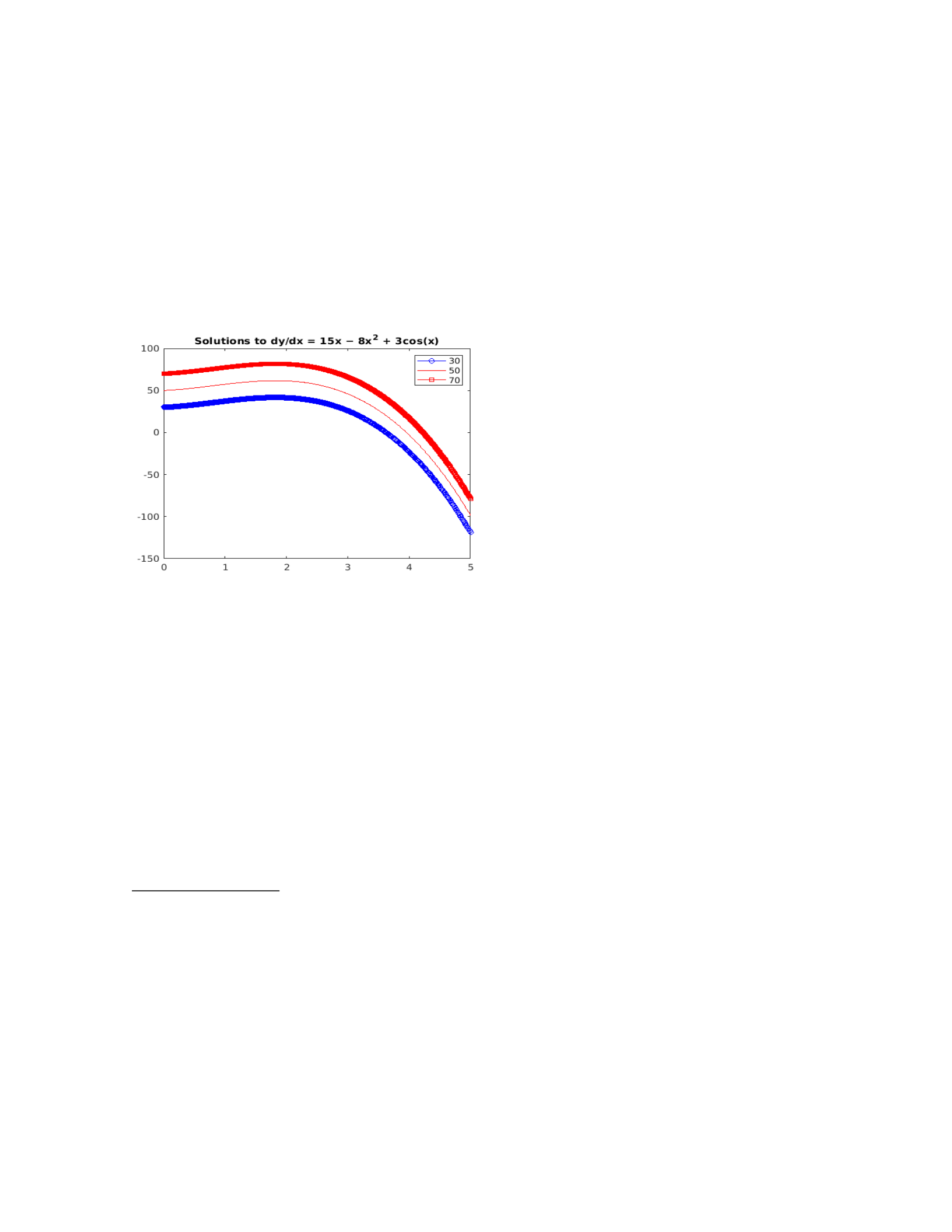
plot (x,y1,'-bo',x,y2,'r-',x,y3,'-rs') % plot the three solutions with
different % line - styles
title ('Solutions to dy/dx = 15x − 8x^2 + 3cos(x)'); % add a title
legend ('30','50','70'); % add a legend
function y = f(x , C )
y = 15*x.^2/2-8*x.^3/3+3*sin(x)+C; % fill -in with the expression for the
general % solution
end
% Print out the code for your created M-file (do NOT submit M-file
% separately).
type 'ex5.m'
% Run your M-file--i.e., execute the M-file.
run 'ex5.m'
%% Exercise 6
% Part (a)
% Define g as anonymous function.
g =@(x,y)(x.^2./y.^4 + cos((7*x.*exp(5*y)))/(x.^3 + 3))
% Evaluate g at the given values of x and y
g(-8,8)
g =
function_handle with value:
@(x,y)(x.^2./y.^4+cos((7*x.*exp(5*y)))/(x.^3+3))
ans =
0.0175

%%
% Part (b)
% Clear the function g out of the workspace.
clear g;
% Print out g.m contents.
type 'g.m'
% Evaluate g at the given values of x and y
%% The End!!!
g(-8,8)
ans =
0.0175
LaB 2
%% Lab 2 - Your Name - MAT 275 Lab
%% Exercise 1
% Part (a)
%%
% Part(b)
%%
% Part (c)
% NOTE: Use the "backslash" command. NOT the division operator "/".
%%
% Part (d)
%%

% Part (e)
%%
% Part (f)
%% Exercise 2
% Part (a)
% NOTE: We must create separate function M-files here. The function will
% require input variables. Therefore, you cannot use "run" to execute the
% function. You must invoke it by providing values for the input
variables.
% Name the function geomsum1. Then complete the following.
% NOTE: You MUST comment each line of code in you M-file similar to how I
% comment each line of code in this script file. You may choose your own
% style of documentation, but make sure it is consistent throughout the
% semester and thoroughly explains what the code is doing. Further, you
% should have a comment at the beginning of each function file explaining
% what the function does. I WILL MARK OFF POINTS otherwise.
% Display contents of geomsum1 M-file.
type 'geomsum1.m'
% Assign values to input variables.
r = 4/5;
a = 9;
n = 11;
% NOTE: Do NOT define r,a, or n inside the function file. This defeats
the
% purpose of requiring input arguments.
% Compute geometric sum for specified values of r,a, and n.
geomsum1(4/5,9,11)
%%
% Part (b)
type 'geomsum2.m'

geomsum2(4/5,9,11)
% NOTE: MATLAB has several built in functions. Here, we want to use the
% built-in function "sum" to compute the same geometric sum as computed
in
% part (a). The "sum" function takes a vector as input and sums its
% elements. Hence, we must create a vector containing all the terms of
the
% sum we wish to compute and pass that vector as input to the sum
function.
% Type "help sum" in command window for more info.
% Don't forget: the name of your function should be geomsum2
%% Exercise 3
% Part (a)
% NOTE: When the protocol says to write a script file, you do not need to
% create a separate M-file. This main file is a script file and you can
% simply write the list of commands here. Please refer to the second
% example on page 5 before attempting this problem.
% Initiate product P.
P = 1;
% Define starting iteration index.
m = 2;
% Define stepsize of iteration.
k = 2;
% Define ending iteration index.
n = 18;
% Compute product.
for i = m:k:n
P = P*i % muliply P by next element at each iteration (suppress output)
end
% Display product.
P
% NOTE: i = m:k:n is also a vector! A for-loop essentially iterates
through
% each element of a vector. Keep this in mind for part (b).

% NOTE: Type "help for" in the command window for more info.
%%
% Part (b)
P = prod(2:2:18)
% NOTE: Emphasis on the part where it says "SINGLE COMMAND." That means
ONE
% line of code. The "prod" function is another built-in function that,
% similar to "sum", takes in a vector as input, yet computes the product
of
% all the elements of the input vector. So, we need to create a vector
% containing all the numbers between 1 and 15 with a stepsize of 2. Which
% vector declaration method is best when we know the stepsize? Also, in
% order to compute the product in a single command, we must declare the
% vector INSIDE the prod command as an input argument, as opposed to x =
% vector, prod(x). Instead, we do prod(vector). Type "help prod" in the
% command window for more info.
%% Exercise 4
% NOTE: When the protocol says to write a script file, you do not need to
% create a separate M-file. This main file is a script file and you can
% simply write the list of commands here. Refer to second example on page
7
% of protocol before attempting this exercise.
% Initiate variables.
power = 1;
k = 0; % initiate counter
% Initialize the vector v to the empty vector
v = [];
% Compute powers and store in v.
while power < 10000 % specify condition of while-loop: stop iterating
once
% condition is no longer satisfied
v(k) = power; % evaluate kth entry of the vector v
k = k+1; % increment counter k
power = 2^k % compute next value of power at each iteration
end
% Display vector v.

v
<code>
%% Exercise 5
% NOTE: Here, we must create a separate function M-file f that accepts
one
% input argument, a value of the variable x. You may want to start
creating
% a new folder for each lab as we will be using f multiple times to
define
% different functions. Please refer to the example on the last page of
the
% protocol before attempting this problem.
% Display contents of function f M-file.
type 'f.m'
% Evaluate f at the given vaue of x.
<code>
% Evaluate f at the given value of x.
<code>
% Evaluate f at the given value of x.
<code>
% Evaluate f at the given value of x.
<code>
% Evaluate f at the given value of x.
<code>
% Evaluate f at the given value of x.
<code>

