



Lab 5 - Abisai Villalobos - MAT 275 Lab
The Mass-Spring System
Exercise 1
Part (a)
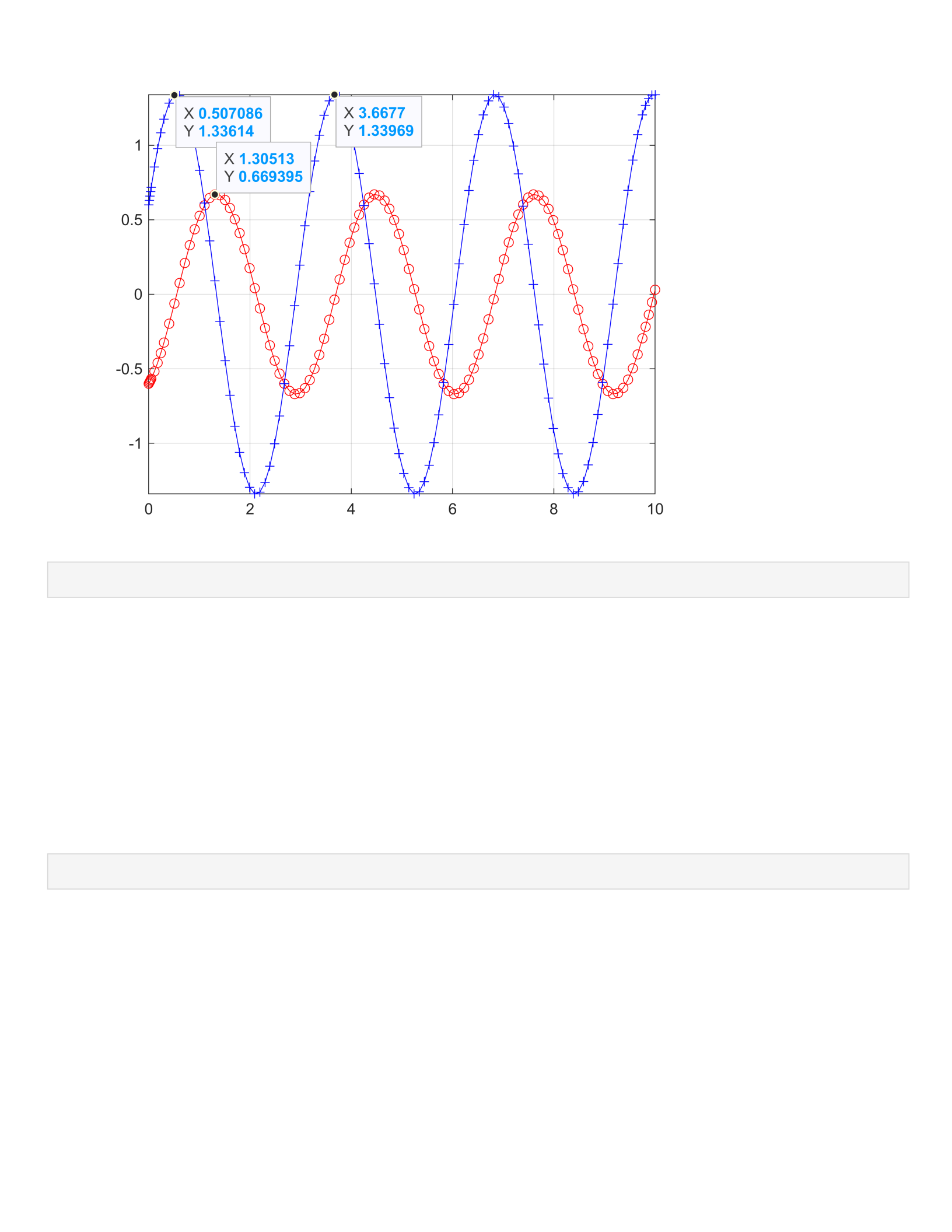
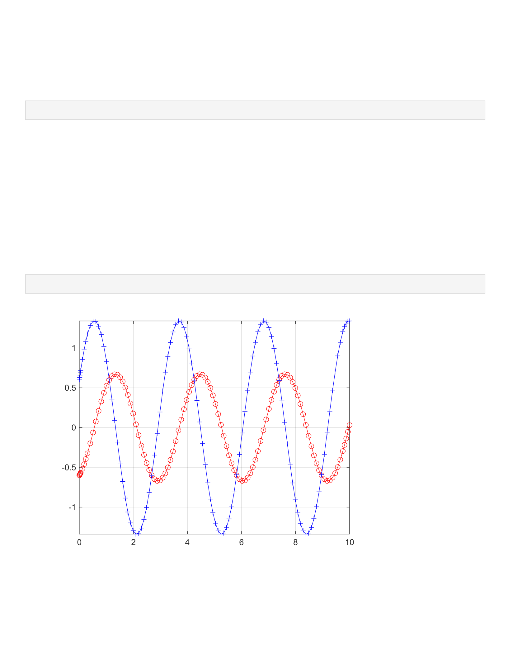
The curve that represents y=y(t) is the red dotted line. This shows its oscillation from (0,-0.6) which is given by
the initial condition.
Part (b)
The period is greater than the value of 3 in this exercise. Using the given values of m and k we solve for w0,
which equals to 2 (sqrt of k/m). The value of the period is equal to pi (2pi/2).
Part (c)
By looking at the consistency of the graph and the fact that its in simple harmonic motion, due to its nature it will
never stop or come to rest because it continously oscillates around its equilibrium position. It will never reach 0.
Part (d)
The amplitude is 0.60.
Part (e)
t=.51
v = 1.34
t=3.67
v=1.34
The maximum velocity is 1.34 m/s at 0.51 seconds.
Part (f)
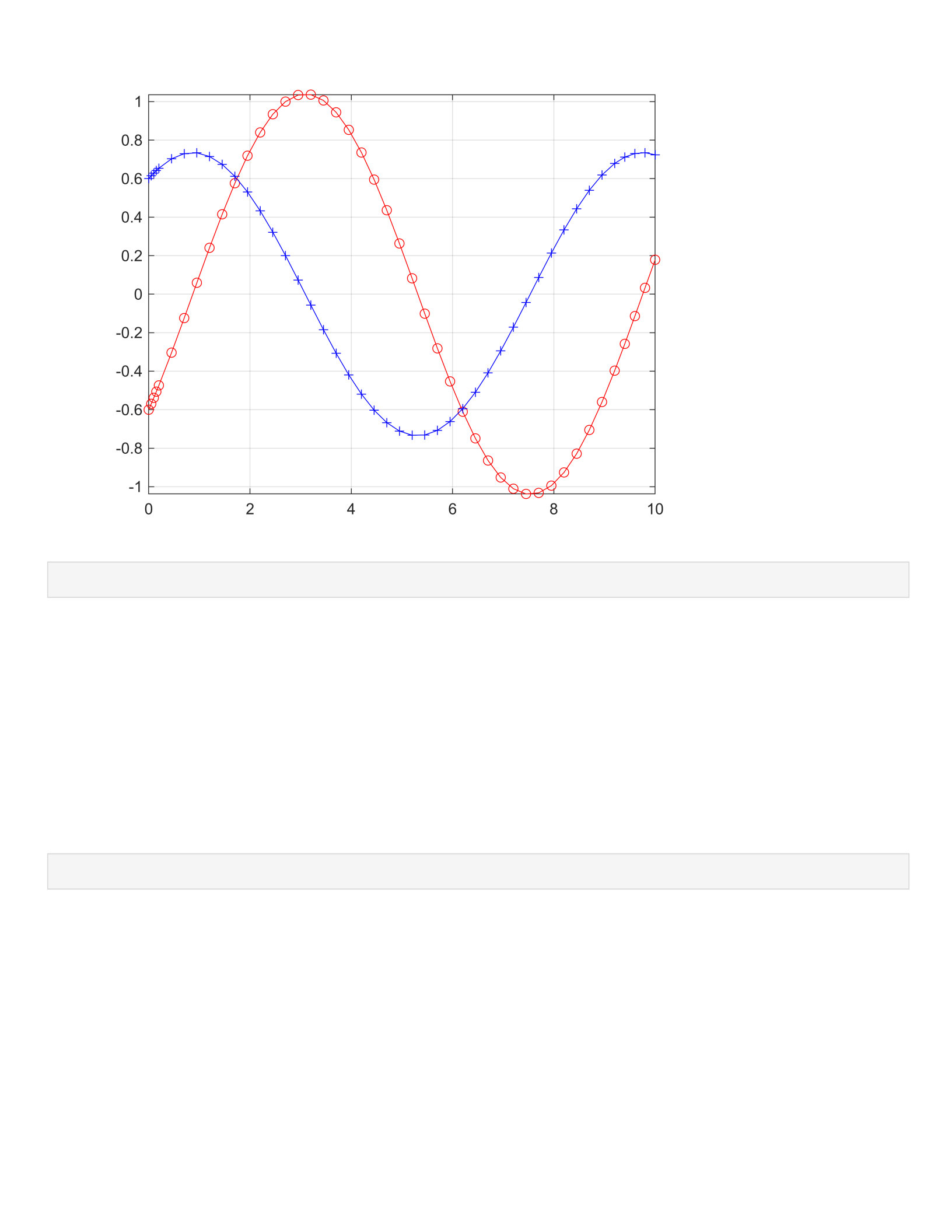
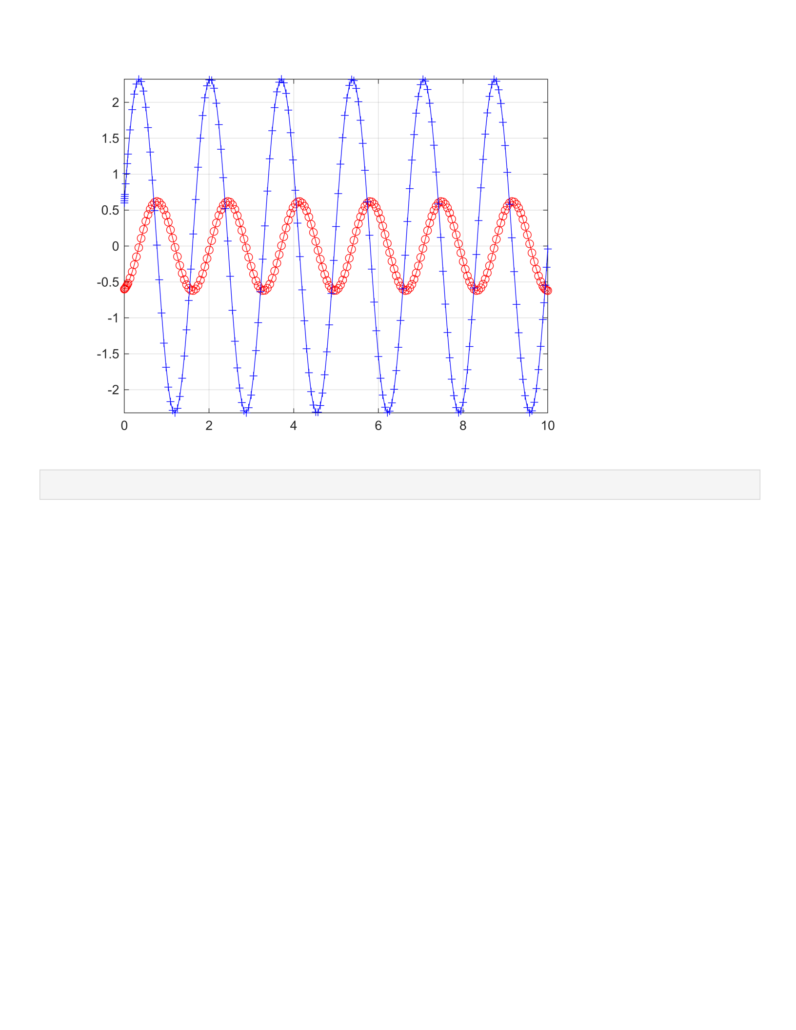
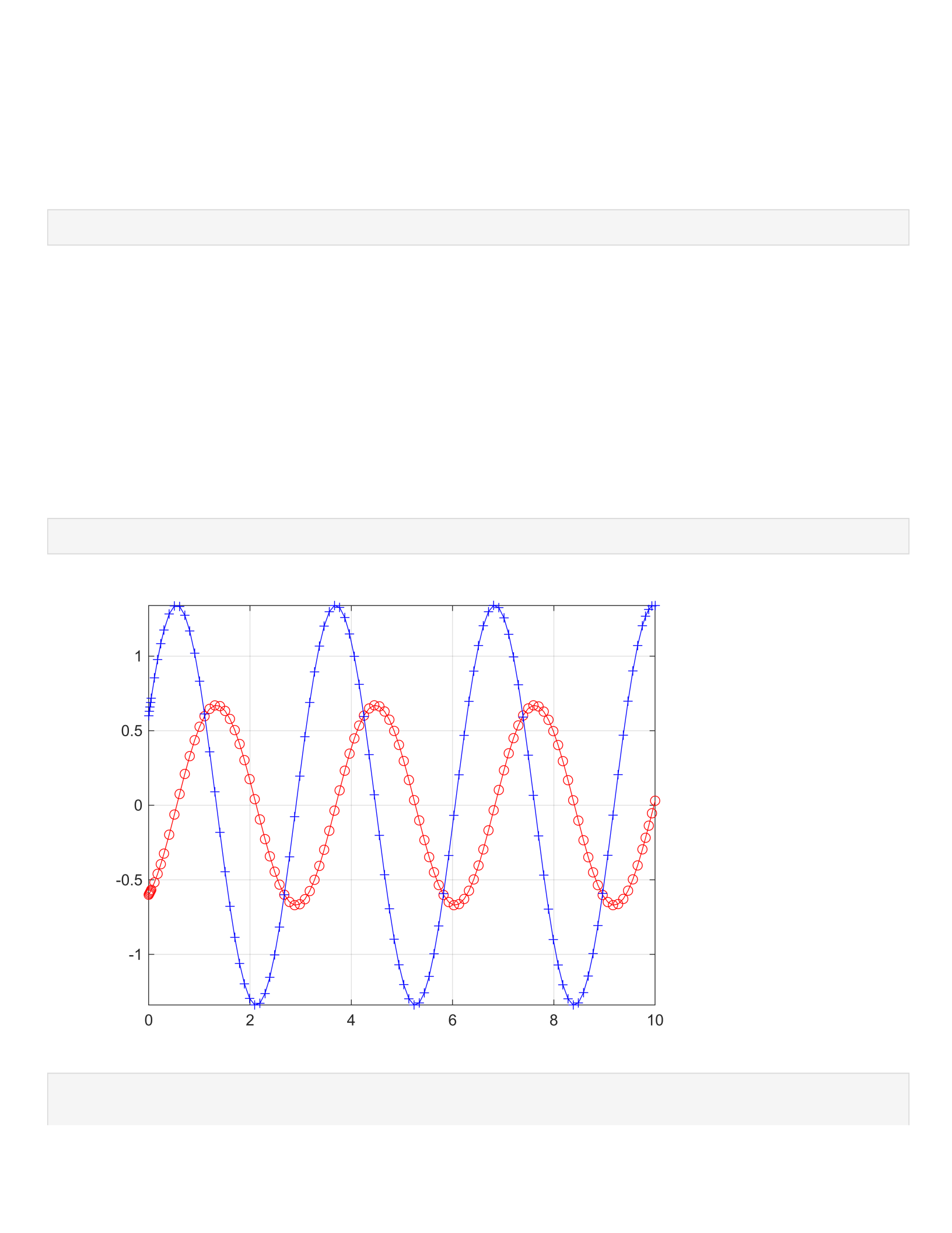
Run LAB05ex1 with the given values of m and k. Include the two distinct graphs, each with y(t) and v(t) plotted.
Comment on the results.
LAB05ex1
1
type lab05ex1.m
clear all; % clear all variables
m = 1; % mass [kg]
k = 4; % spring constant [N/m]
omega0 = sqrt(k/m);
y0 =-0.6; v0 = 0.6; % initial conditions
[t,Y] = ode45(@f,[0,10],[y0,v0],[],omega0); % solve for 0<t<10
y = Y(:,1); v = Y(:,2); % retrieve y, v from Y
figure(1); plot(t,y,'ro-',t,v,'b+-');% time series for y and v
grid on; axis tight;
%---------------------------------------------------
function dYdt = f(t,Y,omega0); % function defining the DE
y = Y(1); v = Y(2);
dYdt=[ v ; - omega0^2*y ];
end
LAB05ex1a
2
type lab05ex1a.m
clear all; % clear all variables
m = 8; % mass [kg]
k = 4; % spring constant [N/m]
omega0 = sqrt(k/m);
y0 =-0.6; v0 = 0.6; % initial conditions
[t,Y] = ode45(@f,[0,10],[y0,v0],[],omega0); % solve for 0<t<10
y = Y(:,1); v = Y(:,2); % retrieve y, v from Y
figure(1); plot(t,y,'ro-',t,v,'b+-');% time series for y and v
grid on; axis tight;
%---------------------------------------------------
function dYdt = f(t,Y,omega0); % function defining the DE
y = Y(1); v = Y(2);
dYdt=[ v ; - omega0^2*y ];
end
LAB05ex1b
3
type LAB05ex1b.m
clear all; % clear all variables
m = 1; % mass [kg]
k = 14; % spring constant [N/m]
omega0 = sqrt(k/m);
y0 =-0.6; v0 = 0.6; % initial conditions
[t,Y] = ode45(@f,[0,10],[y0,v0],[],omega0); % solve for 0<t<10
y = Y(:,1); v = Y(:,2); % retrieve y, v from Y
figure(1); plot(t,y,'ro-',t,v,'b+-');% time series for y and v
grid on; axis tight;
%---------------------------------------------------
function dYdt = f(t,Y,omega0); % function defining the DE
y = Y(1); v = Y(2);
dYdt=[ v ; - omega0^2*y ];
end
Comment: An object's velocity reduces as its mass increases, and inversely also holds true. However, because
of the equation w^2=k/m, the velocity likewise increases as the spring constant does. Consequently, it is evident
that the mass and the spring constant are inverse. Additionally, relative to a system with a lower frequency rate
or a system with a higher mass, an object traveling at a faster velocity covers a longer distance in the same
amount of time as the frequency increases.
4
Exercise 2
Part (a)
add commands to LAB05ex1 to compute and plot E(t). Then use ylim([~,~]) to change the yaxis limits. Include
the code, at least one plot of E(t) and a comment.
type LAB05ex1_2.m
clear all; % clear all variables
m = 1; % mass [kg]
k = 4; % spring constant [N/m]
omega0 = sqrt(k/m);
y0 =-0.6; v0 = 0.6; % initial conditions
[t,Y] = ode45(@f,[0,10],[y0,v0],[],omega0); % solve for 0<t<10
y = Y(:,1); v = Y(:,2); % retrieve y, v from Y
E = 1/2*m*v.^2 + 1/2 * k*y.^2;
figure(1); plot(t,y,'ro-',t,v,'b+-');% time series for y and v
grid on; axis tight;
%---------------------------------------------------
function dYdt = f(~,Y,omega0); % function defining the DE
y = Y(1); v = Y(2);
dYdt=[ v ; - omega0^2*y ];
end
LAB05ex1_2
E = round(E,1);
5
figure(2);
plot(t,E);
grid on; axis tight;
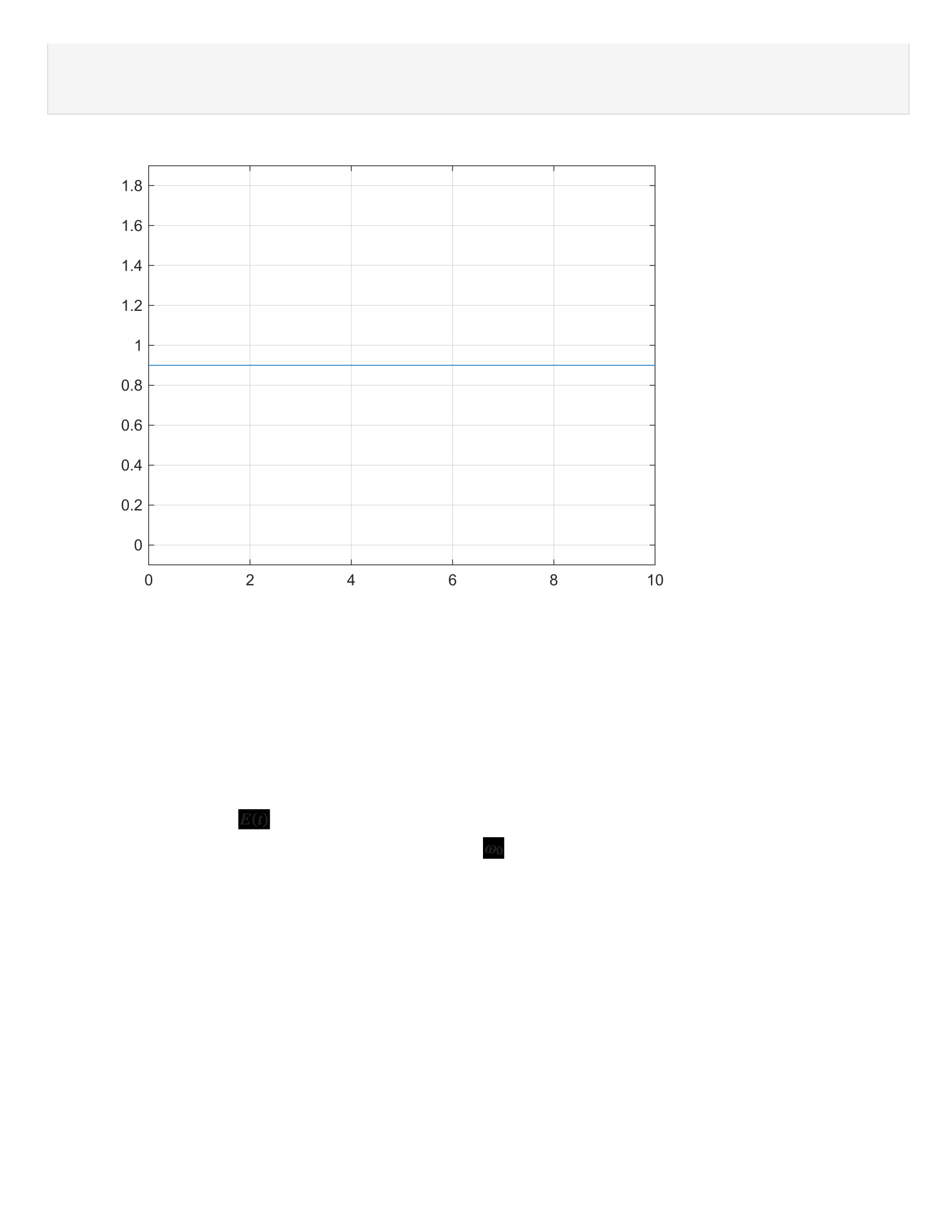
Comment: The kinetic and potential energy of a mass-spring system is depicted in the graph. The existence and
conservation of energy in this instance are demonstrated by the straight line with slope = 0.
Part (b)
write out main steps here:
•first differentiate with respect to t using the chain rule.
•then make substitutions using the expression for and using the differential equation
E(t)=(1/2)mv^2+(1/2)ky^2
(dE/dt)=(1/2)m(2v)(dv/dt)+(1/2)k(2y)(dy/dt)
(dE/dt)=mv(dv/dt)+ky(dy/dt)
m(dv.dt)=-ky
(dy/dt)=v
(dE/dt)=(-ky)v+(ky)v
6
(dE/dt)=0
Part (c)
Include modified M-file (or the added lines), plot and comment
type LAB05ex1_3.m
clear all; % clear all variables
m = 1; % mass [kg]
k = 4; % spring constant [N/m]
omega0 = sqrt(k/m);
y0 =-0.6; v0 = 0.6; % initial conditions
[t,Y] = ode45(@f,[0,10],[y0,v0],[],omega0); % solve for 0<t<10
y = Y(:,1); v = Y(:,2); % retrieve y, v from Y
figure(1); plot(t,y,'ro-',t,v,'b+-');% time series for y and v
grid on; axis tight;
figure(2);
plot(y,v);
%---------------------------------------------------
function dYdt = f(~,Y,omega0); % function defining the DE
y = Y(1); v = Y(2);
dYdt=[ v ; - omega0^2*y ];
end
LAB05ex1_3
7
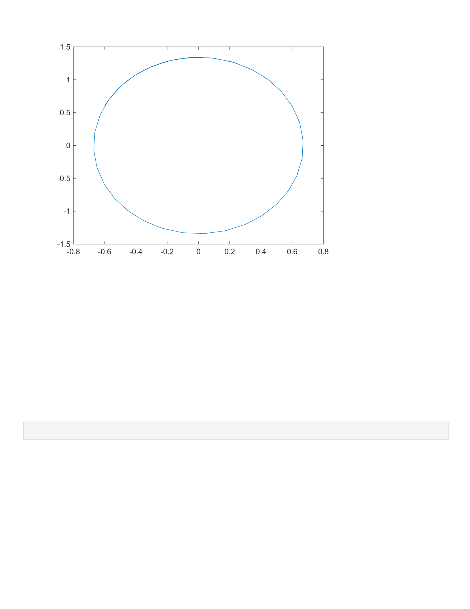
Comment: When we look at the diagram's circular system orientation, we can see that it never touches the
origin. This demonstrates the existence of energy conservation even more. It will always be circular because the
total energy is constant.
Exercise 3
Part (a)
modify the system of equations in LAB05ex2 write the t value. If you use the given matlab commands you will
need to explain them.
type LAB05ex2.m
clear all; % clear all variables
m = 1; % mass [kg]
k = 4; % spring constant [N/m]
c = 1; % friction coefficient [Ns/m]
omega0 = sqrt(k/m); p = c/(2*m);
y0 =-0.6; v0 = 0.6; % initial conditions
[t,Y] = ode45(@f,[0,10],[y0,v0],[],omega0, p); % solve for 0<t<10
y = Y(:,1); v = Y(:,2); % retrieve y, v from Y
figure(1); plot(t,y,'ro-',t,v,'b+-');% time series for y and v
grid on; axis tight;
%---------------------------------------------------
function dYdt = f(t,Y,omega0,p); % function defining the DE
y = Y(1); v = Y(2);
8
dYdt=[ v ; -2*p*v-omega0^2*y]; % fill-in dv/dt
end
LAB05ex2
for i=1: length (y)
M(i)= max(abs(y(i:end )));
end
i = find (M <0.04);
i = i(1)
i = 57
disp (['|y| <0.04 for t > t1 with ' num2str(t(i-1)) '< t1 <' num2str(t(i))])
|y| <0.04 for t > t1 with 4.9788< t1 <5.0712
By using the given MATLAB command, I found t1 is at 57 seconds.
Part (b)
write t value and max V value; note: velocity magnitude is like absolute value!
for i=1: length (v)
M(i)= max(abs(v(i:end )));
end
i = find (M <0.04);
9

i = i(1)
i = 65
disp (['|v| <0.04 for t > t1 with ' num2str(t(i-1)) '< t1 <' num2str(t(i))])
|v| <0.04 for t > t1 with 5.7936< t1 <5.8913
By using the given MATLAB command, I found the maximum velocity when t=5.7936 at
65m/s.
Part (c)
include 3 figures here + comments. use title('text') to attach a title to the figure
type LAB05ex2a.m
clear all; % clear all variables
m = 1; % mass [kg]
k = 4; % spring constant [N/m]
c = 2; % friction coefficient [Ns/m]
omega0 = sqrt(k/m); p = c/(2*m);
y0 =-0.6; v0 = 0.6; % initial conditions
[t,Y] = ode45(@f,[0,10],[y0,v0],[],omega0, p); % solve for 0<t<10
y = Y(:,1); v = Y(:,2); % retrieve y, v from Y
figure(1); plot(t,y,'ro-',t,v,'b+-');% time series for y and v
grid on; axis tight;
%---------------------------------------------------
function dYdt = f(t,Y,omega0,p); % function defining the DE
y = Y(1); v = Y(2);
dYdt=[ v ; -2*p*v-omega0^2*y]; % fill-in dv/dt
end
LAB05ex2a
10
type LAB05ex2b.m
clear all; % clear all variables
m = 1; % mass [kg]
k = 4; % spring constant [N/m]
c = 4; % friction coefficient [Ns/m]
omega0 = sqrt(k/m); p = c/(2*m);
y0 =-0.6; v0 = 0.6; % initial conditions
[t,Y] = ode45(@f,[0,10],[y0,v0],[],omega0, p); % solve for 0<t<10
y = Y(:,1); v = Y(:,2); % retrieve y, v from Y
figure(1); plot(t,y,'ro-',t,v,'b+-');% time series for y and v
grid on; axis tight;
%---------------------------------------------------
function dYdt = f(t,Y,omega0,p); % function defining the DE
y = Y(1); v = Y(2);
dYdt=[ v ; -2*p*v-omega0^2*y]; % fill-in dv/dt
end
LAB05ex2b
11
type LAB05ex2c.m
clear all; % clear all variables
m = 1; % mass [kg]
k = 4; % spring constant [N/m]
c = 12; % friction coefficient [Ns/m]
omega0 = sqrt(k/m); p = c/(2*m);
y0 =-0.6; v0 = 0.6; % initial conditions
[t,Y] = ode45(@f,[0,10],[y0,v0],[],omega0, p); % solve for 0<t<10
y = Y(:,1); v = Y(:,2); % retrieve y, v from Y
figure(1); plot(t,y,'ro-',t,v,'b+-');% time series for y and v
grid on; axis tight;
%---------------------------------------------------
function dYdt = f(t,Y,omega0,p); % function defining the DE
y = Y(1); v = Y(2);
dYdt=[ v ; -2*p*v-omega0^2*y ]; % fill-in dv/dt
end
LAB05ex2c
12
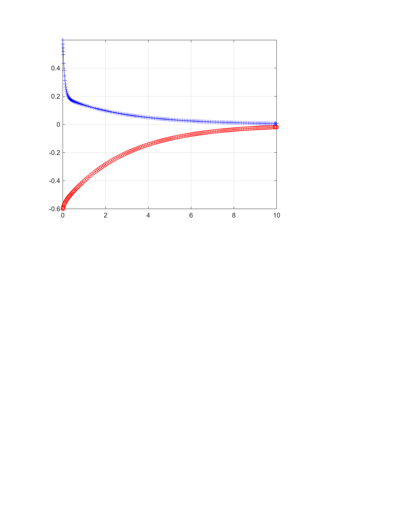
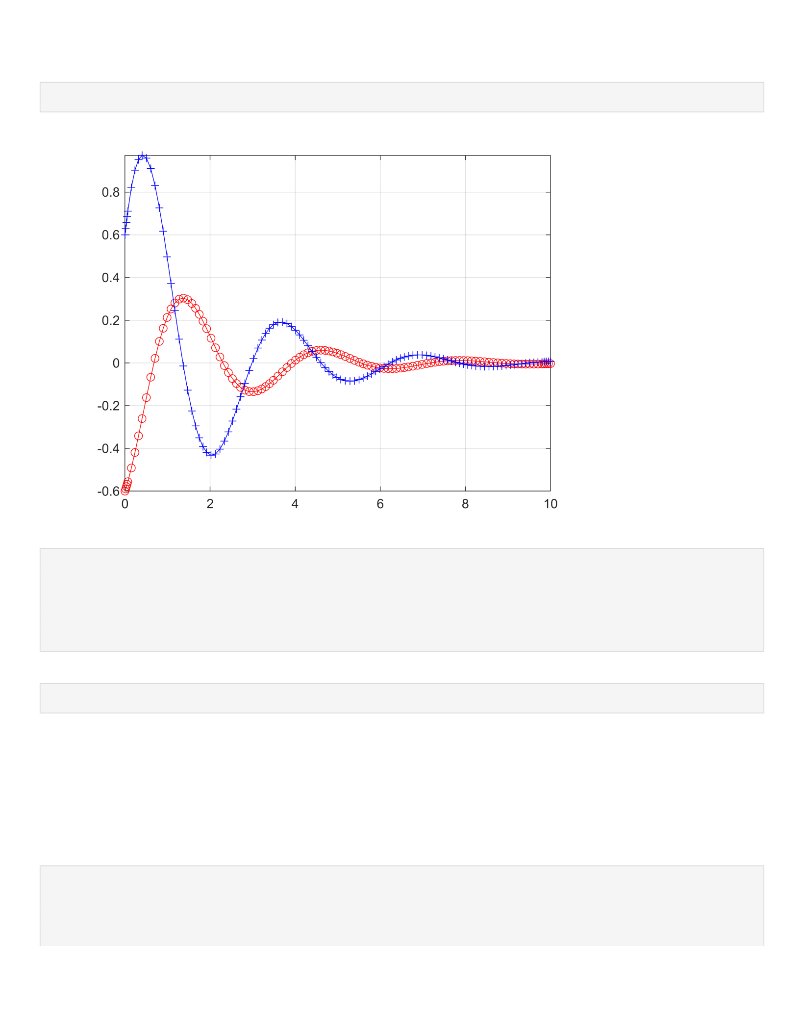
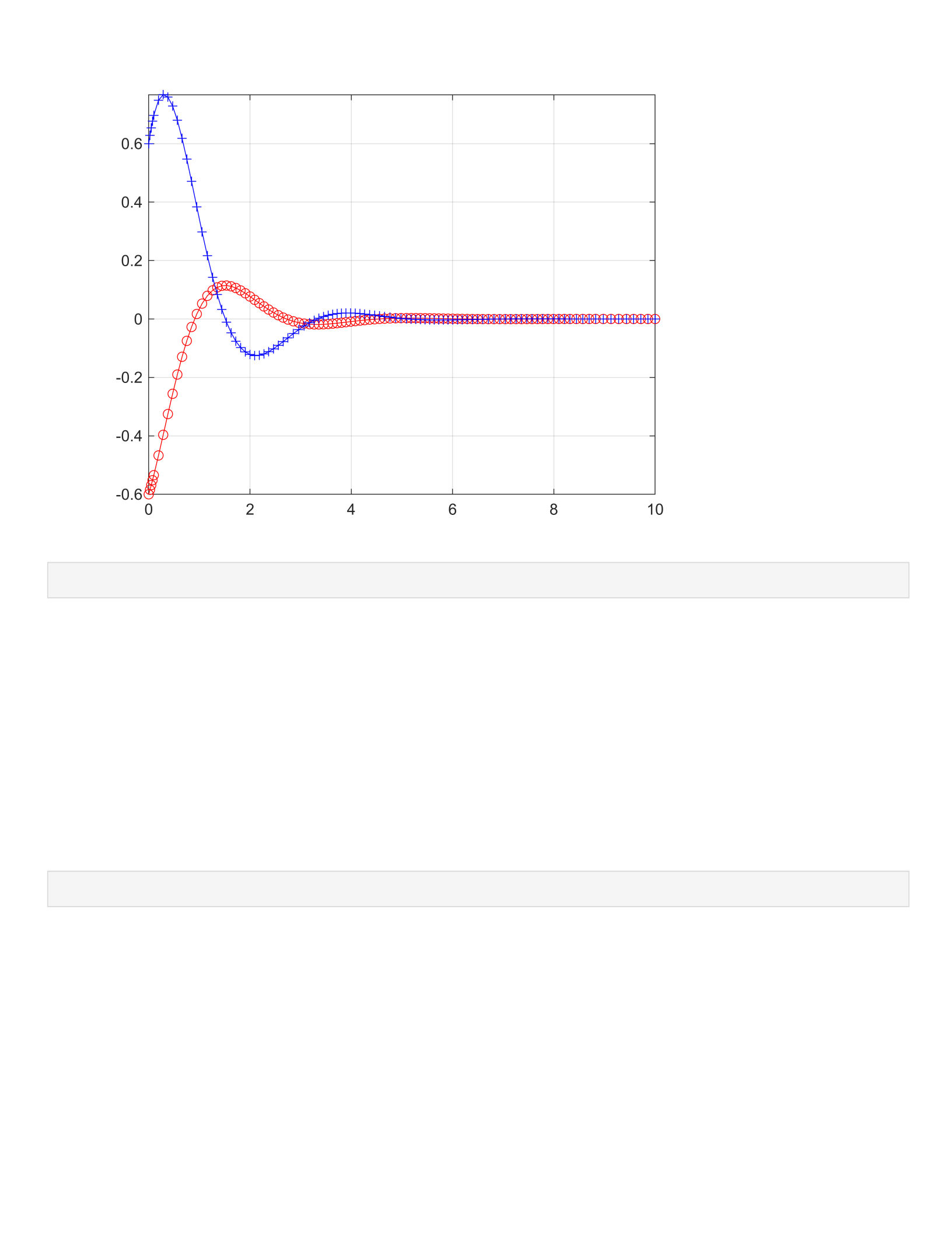
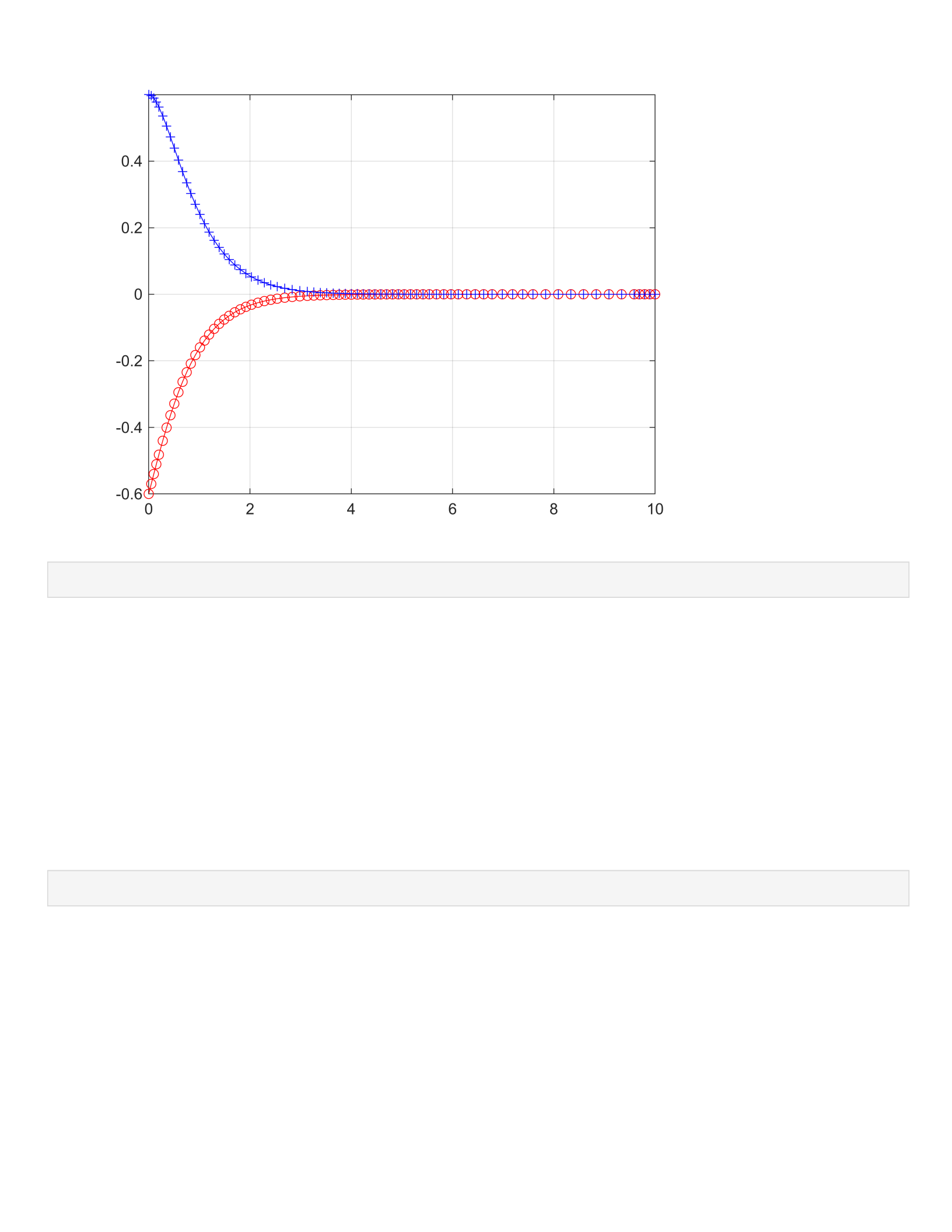
Comments: The number of oscillations in a given period of time reduces when the
damping constant is raised. The amount of energy in a system is decreased when
damping force is applied. Therefore, the more robust the damping force, the less
oscillations will occur over time.
Part (d)
What needs to happen (in terms of the characteristic equation) in order for there to be no oscillations? Impose a
condition on the characteristic equation to find the critical c value. Write out main steps
With no oscillations, we can set up an equation equal to 0 in order to find the c constant.
(c^2)-4mk=0
c=sqrt(4mk)
m=1, k=4
c=sqrt(4*1*4)
c=4
Exercise 4
13
Part (a)
Include the completed M-file, 1 figure and comment
type LAB05ex2_exercise4.m
clear all; % clear all variables
m = 1; % mass [kg]
k = 4; % spring constant [N/m]
c = 1; % friction coefficient [Ns/m]
omega0 = sqrt(k/m); p = c/(2*m);
y0 =-0.6; v0 = 0.6; % initial conditions
[t,Y] = ode45(@f,[0,10],[y0,v0],[],omega0, p); % solve for 0<t<10
y = Y(:,1); v = Y(:,2); % retrieve y, v from Y
E = 0.5*m*v.^2+1/2*k*y.^2;
E = round(E,1);
figure(2); plot(t,E);% time series for y and v
grid on; axis tight;
ylim([-0.8,0.8])
%---------------------------------------------------
function dYdt = f(t,Y,omega0,p); % function defining the DE
y = Y(1); v = Y(2);
dYdt=[ v ; -2*p*v - omega0^2*y]; % dy/dt = v, dv/dt = -2pv - omega0^2*y
end
LAB05ex2_exercise4
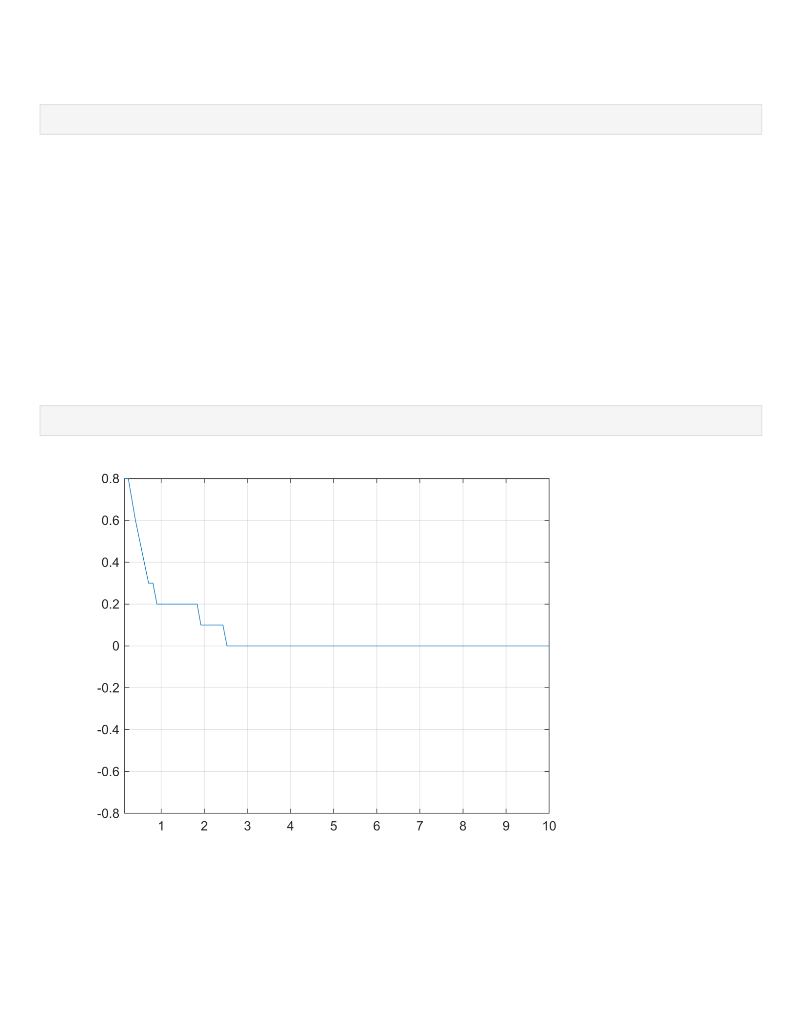
Comment: This implies that this system does not conserve energy. The total energy in
a conservative system would normally oscillate if it were a mass-spring or pendulum
with no energy loss. Energy dissipation is implied by the stepwise drop to zero, which
could be brought on by damping or another non-conservative cause.
14

Part (b)
Again find using the chain rule and make substitutions based on the differential equation. You should reach
an expression for which is in terms of
(dE/dt)=(1/2)m(2v)(dv/dt)+(1/2)k(2y)(dy/dt)
(dE/dt)=mvv'+kyy'
(dE/dt)=v(-c*y'-k*y+k*y)
c=4
(dE/dt)=-4vy'
Part (c)
Include M-file (or added lines), one figure and comment.
type LAB05ex2_exercise4b.m
clear all; % clear all variables
m = 1; % mass [kg]
k = 4; % spring constant [N/m]
c = 1; % friction coefficient [Ns/m]
omega0 = sqrt(k/m); p = c/(2*m);
y0 =-0.6; v0 = 0.6; % initial conditions
[t,Y] = ode45(@f,[0,10],[y0,v0],[],omega0, p); % solve for 0<t<10
y = Y(:,1); v = Y(:,2); % retrieve y, v from Y
E = 0.5*m*v.^2+1/2*k*y.^2;
figure(2); plot(y,v);% time series for y and v
grid on; axis tight;
ylim([-0.8,0.8])
%---------------------------------------------------
function dYdt = f(t,Y,omega0,p); % function defining the DE
y = Y(1); % displacement
v = Y(2); % velocity
dYdt = [v; -2*p*v - omega0^2*y]; % dy/dt = v, dv/dt = -2pv - omega0^2*y
end
LAB05ex2_exercise4b
15
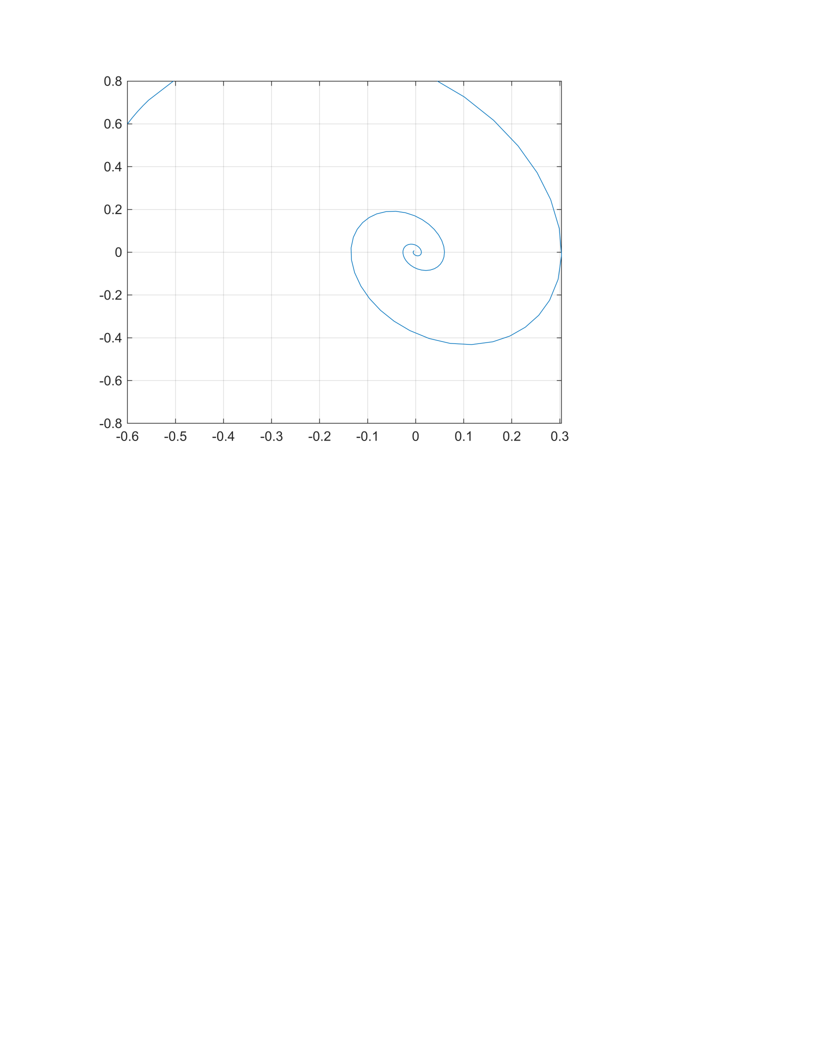
Comment: When the spiral reaches the origin, the motion finally reaches the state of equilibrium. This
indicates that the system is losing energy. The motion will diminish as the energy decreases.
16

11/10/24 11:13 PM C:\Users\Dell...\LAB05ex2_exercise4b.m 1 of 1
clear all; % clear all variables
m = 1; % mass [kg]
k = 4; % spring constant [N/m]
c = 1; % friction coefficient [Ns/m]
omega0 = sqrt(k/m); p = c/(2*m);
y0 =-0.6; v0 = 0.6; % initial conditions
[t,Y] = ode45(@f,[0,10],[y0,v0],[],omega0, p); % solve for 0<t<10
y = Y(:,1); v = Y(:,2); % retrieve y, v from Y
E = 0.5*m*v.^2+1/2*k*y.^2;
figure(2); plot(y,v);% time series for y and v
grid on; axis tight;
ylim([-0.8,0.8])
%---------------------------------------------------
function dYdt = f(t,Y,omega0,p); % function defining the DE
y = Y(1); % displacement
v = Y(2); % velocity
dYdt = [v; -2*p*v - omega0^2*y]; % dy/dt = v, dv/dt = -2pv - omega0^2*y
end

11/10/24 11:13 PM C:\Users\Dell ...\LAB05ex2_exercise4.m 1 of 1
clear all; % clear all variables
m = 1; % mass [kg]
k = 4; % spring constant [N/m]
c = 1; % friction coefficient [Ns/m]
omega0 = sqrt(k/m); p = c/(2*m);
y0 =-0.6; v0 = 0.6; % initial conditions
[t,Y] = ode45(@f,[0,10],[y0,v0],[],omega0, p); % solve for 0<t<10
y = Y(:,1); v = Y(:,2); % retrieve y, v from Y
E = 0.5*m*v.^2+1/2*k*y.^2;
E = round(E,1);
figure(2); plot(t,E);% time series for y and v
grid on; axis tight;
ylim([-0.8,0.8])
%---------------------------------------------------
function dYdt = f(t,Y,omega0,p); % function defining the DE
y = Y(1); v = Y(2);
dYdt=[ v ; -2*p*v - omega0^2*y]; % dy/dt = v, dv/dt = -2pv - omega0^2*y
end

11/10/24 11:12 PM C:\Users\Dell Precision...\LAB05ex2c.m 1 of 1
clear all; % clear all variables
m = 1; % mass [kg]
k = 4; % spring constant [N/m]
c = 12; % friction coefficient [Ns/m]
omega0 = sqrt(k/m); p = c/(2*m);
y0 =-0.6; v0 = 0.6; % initial conditions
[t,Y] = ode45(@f,[0,10],[y0,v0],[],omega0, p); % solve for 0<t<10
y = Y(:,1); v = Y(:,2); % retrieve y, v from Y
figure(1); plot(t,y,'ro-',t,v,'b+-');% time series for y and v
grid on; axis tight;
%---------------------------------------------------
function dYdt = f(t,Y,omega0,p); % function defining the DE
y = Y(1); v = Y(2);
dYdt=[ v ; -2*p*v-omega0^2*y ]; % fill-in dv/dt
end

11/10/24 11:12 PM C:\Users\Dell Precision...\LAB05ex2b.m 1 of 1
clear all; % clear all variables
m = 1; % mass [kg]
k = 4; % spring constant [N/m]
c = 4; % friction coefficient [Ns/m]
omega0 = sqrt(k/m); p = c/(2*m);
y0 =-0.6; v0 = 0.6; % initial conditions
[t,Y] = ode45(@f,[0,10],[y0,v0],[],omega0, p); % solve for 0<t<10
y = Y(:,1); v = Y(:,2); % retrieve y, v from Y
figure(1); plot(t,y,'ro-',t,v,'b+-');% time series for y and v
grid on; axis tight;
%---------------------------------------------------
function dYdt = f(t,Y,omega0,p); % function defining the DE
y = Y(1); v = Y(2);
dYdt=[ v ; -2*p*v-omega0^2*y]; % fill-in dv/dt
end

11/10/24 11:12 PM C:\Users\Dell Precision...\LAB05ex2a.m 1 of 1
clear all; % clear all variables
m = 1; % mass [kg]
k = 4; % spring constant [N/m]
c = 2; % friction coefficient [Ns/m]
omega0 = sqrt(k/m); p = c/(2*m);
y0 =-0.6; v0 = 0.6; % initial conditions
[t,Y] = ode45(@f,[0,10],[y0,v0],[],omega0, p); % solve for 0<t<10
y = Y(:,1); v = Y(:,2); % retrieve y, v from Y
figure(1); plot(t,y,'ro-',t,v,'b+-');% time series for y and v
grid on; axis tight;
%---------------------------------------------------
function dYdt = f(t,Y,omega0,p); % function defining the DE
y = Y(1); v = Y(2);
dYdt=[ v ; -2*p*v-omega0^2*y]; % fill-in dv/dt
end

11/10/24 11:11 PM C:\Users\Dell Precision\...\LAB05ex2.m 1 of 1
clear all; % clear all variables
m = 1; % mass [kg]
k = 4; % spring constant [N/m]
c = 1; % friction coefficient [Ns/m]
omega0 = sqrt(k/m); p = c/(2*m);
y0 =-0.6; v0 = 0.6; % initial conditions
[t,Y] = ode45(@f,[0,10],[y0,v0],[],omega0, p); % solve for 0<t<10
y = Y(:,1); v = Y(:,2); % retrieve y, v from Y
figure(1); plot(t,y,'ro-',t,v,'b+-');% time series for y and v
grid on; axis tight;
%---------------------------------------------------
function dYdt = f(t,Y,omega0,p); % function defining the DE
y = Y(1); v = Y(2);
dYdt=[ v ; -2*p*v-omega0^2*y]; % fill-in dv/dt
end

11/10/24 11:10 PM C:\Users\Dell Precisio...\LAB05ex1_3.m 1 of 1
clear all; % clear all variables
m = 1; % mass [kg]
k = 4; % spring constant [N/m]
omega0 = sqrt(k/m);
y0 =-0.6; v0 = 0.6; % initial conditions
[t,Y] = ode45(@f,[0,10],[y0,v0],[],omega0); % solve for 0<t<10
y = Y(:,1); v = Y(:,2); % retrieve y, v from Y
figure(1); plot(t,y,'ro-',t,v,'b+-');% time series for y and v
grid on; axis tight;
figure(2);
plot(y,v);
%---------------------------------------------------
function dYdt = f(~,Y,omega0); % function defining the DE
y = Y(1); v = Y(2);
dYdt=[ v ; - omega0^2*y ];
end

11/10/24 11:09 PM C:\Users\Dell Precisio...\LAB05ex1_2.m 1 of 1
clear all; % clear all variables
m = 1; % mass [kg]
k = 4; % spring constant [N/m]
omega0 = sqrt(k/m);
y0 =-0.6; v0 = 0.6; % initial conditions
[t,Y] = ode45(@f,[0,10],[y0,v0],[],omega0); % solve for 0<t<10
y = Y(:,1); v = Y(:,2); % retrieve y, v from Y
E = 1/2*m*v.^2 + 1/2 * k*y.^2;
figure(1); plot(t,y,'ro-',t,v,'b+-');% time series for y and v
grid on; axis tight;
%---------------------------------------------------
function dYdt = f(~,Y,omega0); % function defining the DE
y = Y(1); v = Y(2);
dYdt=[ v ; - omega0^2*y ];
end

11/10/24 11:09 PM C:\Users\Dell Precision...\LAB05ex1b.m 1 of 1
clear all; % clear all variables
m = 1; % mass [kg]
k = 14; % spring constant [N/m]
omega0 = sqrt(k/m);
y0 =-0.6; v0 = 0.6; % initial conditions
[t,Y] = ode45(@f,[0,10],[y0,v0],[],omega0); % solve for 0<t<10
y = Y(:,1); v = Y(:,2); % retrieve y, v from Y
figure(1); plot(t,y,'ro-',t,v,'b+-');% time series for y and v
grid on; axis tight;
%---------------------------------------------------
function dYdt = f(t,Y,omega0); % function defining the DE
y = Y(1); v = Y(2);
dYdt=[ v ; - omega0^2*y ];
end

11/10/24 11:08 PM C:\Users\Dell Precision...\LAB05ex1a.m 1 of 1
clear all; % clear all variables
m = 8; % mass [kg]
k = 4; % spring constant [N/m]
omega0 = sqrt(k/m);
y0 =-0.6; v0 = 0.6; % initial conditions
[t,Y] = ode45(@f,[0,10],[y0,v0],[],omega0); % solve for 0<t<10
y = Y(:,1); v = Y(:,2); % retrieve y, v from Y
figure(1); plot(t,y,'ro-',t,v,'b+-');% time series for y and v
grid on; axis tight;
%---------------------------------------------------
function dYdt = f(t,Y,omega0); % function defining the DE
y = Y(1); v = Y(2);
dYdt=[ v ; - omega0^2*y ];
end

11/10/24 11:07 PM C:\Users\Dell Precision\...\LAB05ex1.m 1 of 1
clear all; % clear all variables
m = 1; % mass [kg]
k = 4; % spring constant [N/m]
omega0 = sqrt(k/m);
y0 =-0.6; v0 = 0.6; % initial conditions
[t,Y] = ode45(@f,[0,10],[y0,v0],[],omega0); % solve for 0<t<10
y = Y(:,1); v = Y(:,2); % retrieve y, v from Y
figure(1); plot(t,y,'ro-',t,v,'b+-');% time series for y and v
grid on; axis tight;
%---------------------------------------------------
function dYdt = f(t,Y,omega0); % function defining the DE
y = Y(1); v = Y(2);
dYdt=[ v ; - omega0^2*y ];
end

