



Improving the Productivity of Hardware Design
Current practices for digital design largely contrast with the rapid development
techniques that became so popular in software development in the last decade [33,76]. This
has not been a major problem, as performance advances in digital design have largely relied
on technology scaling [44,52]. Dennard’s scaling allowed for performance improvement with
limited power impact [98]. However, as the rate of voltage scaling was reduced–a significant
part due to nearing transistor threshold voltage–power became a major bottleneck to maintain
the accelerated frequency scaling that was key for performance gains [46].
In that scenario, multicore computers emerged as an alternative to keep in-
creasing performance [57]. Since the original multicores were homogeneous, i.e., each core
was a copy of each other, this approach resulted in limited design effort. The move to
multicore systems, however, was a bet on moving the performance improvement efforts from
hardware to software [10]. It soon became clear that multicore alone would not be sufficient
to maintain the levels of performance improvement historically observed by computers [50].
More recently, it became clear that to maintain performance scaling, specialized
hardware would be needed. There are many approaches to specialized, or domainspecific,
hardware. Graphical Processing Units (GPUs) [83] certainly became the most popular type in
this category and have since been applied to a wide variety of application domain.
Nevertheless, using GPUs for compute–while known to improve throughput of some
applications–is not the best case for “specialized” design. Heterogeneous multicores [15] and
accelerator-based architectures [35,72] provide hardware that is more optimized to specific
tasks.
1

While specialized hardware is known to improve both performance and energy
efficiency by orders of magnitude over general purpose hardware [65,93,94], the lack of
flexibility of specialized hardware has proved a challenge for deployment in some cases [94].
Accelerators in Field-Programmable Gate Arrays (FPGAs) provides a more flexible
alternative [94] that allows for changes after deployment, with reduced performance
compared to Application-Specific Integrated Circuits (ASICs) but better performance than
general purpose computing.
For both ASIC and FPGA accelerators alike, design techniques and synthesis
Table 1.1: Hardware design methodologies largely contrast with modern software
development, based on agile techniques that allow for several iterations over a relatively
small amount of time. The table shows one software project (LGraph), one hardware project
(Boom) and the runtimes to compile/synthesize them in full or a small change in each.
Codebase Lines of code Task Runtime (s) Small change time (s)
LGraph [92] 1.5M Compilation 82.6 6.7
Boom [14] 0.5M Synthesis 996 948
Boom [14] 0.5M Place & Route 1314 1103
times are major bottlenecks [93]. These bottlenecks become more prominent as specialized
hardware becomes more broadly accessible and domain specialists–that are not necessarily
hardware designers–become interested in using specialized hardware. It is clear that
“compile” time, in a broad sense here, is very different when targeting software or hardware,
which is a initial barrier to domain specialists used to software compilation. Hardware
compilation includes synthesis, placement and routing. To get a rough idea of how those
times vary, I compare the runtimes for two projects, 1 LGraph, a software project, and Boom,
a hardware core. Note that even though those are arguably not representative of all software
and hardware designs, this comparison provides an idea of timescales seen in both worlds.
1 Archlinux Server with 32 Intel Xeon E5-2689 cores, running at 2.6GHz, with 256Gb of RAM. Compilation
with Clang 7.0 and Synthesis, Placement and Routing with Xilinx Vivado 2017.2.
2

Also, even though LGraph compiles 3× more code than Boom, compiling LGraph is sill over
10× faster than just synthesizing Boom.
Recently, researchers have focused on improving the productivity of hardware
design in multiple fronts. New abstractions and Hardware Description Languages (HDLs),
such as Chisel [16], PyMTL [74], Pyrope [101], among others, have been created to increase
the expressiveness of code describing hardware. Those and others try to provide features
already common in modern programming languages for hardware designers, while
maintaining the engineer in control of the resulting circuit. Chip generators are also a
framework for improving productivity by providing a complete sandbox that can be reused
and specialized as needed, some examples are Rocket Chip [12], Celerity [3], OpenPiton
[17], and FabScalar [32].
Lee et al. proposed an agile approach for building chips using the Rocket Chip
generator as the main building block [70]. They introduced the concept of “tapeins,” a
complete chip specification with a small number of added features as a base for iteration. The
main advantage of this approach is to split validation into multiple iterations, reducing the
amount of features that need to be validated at a given cycle. This flow tries to escape the
traditional waterfall approach of hardware development in favor of a iterative flow, usually
seen in agile methodologies for software.
However, some of the underlying problems still persist and have not been
addressed. Due to the need of synthesis, each iteration, either for functionality or timing
targets, remains long. Moreover, timing closure still requires multiple iterations, even if those
3

are more evenly distributed during design time, as opposed to concentrated closer to the end
of the cycle.
Current methodologies for digital design are based on either the fixed cycle
paradigm, where cycle time target and pipeline depth are set early in the design phase, or on
High Level Synthesis (HLS) [36, 54, 95], where scheduling is done in an initial pass before
Register Transfer Level (RTL) generation. In both those cases, the timing characteristics of
the design are only accurately known after synthesis, placement and routing, which are time
consuming tasks. Meeting a desired cycle time requires numerous long iterations between
design and implementation [87]. Existing Electronic Design Automation (EDA) tools allow
automatic optimizations such as gate sizing, retiming and time borrowing, but for a
synchronous system, such transformations preserve cycle accuracy [88] and thus are limited
by the existing pipeline stages already present in the design [53].
Moreover, to fully assess the impact of pipelining, or any other transformation on a
circuit, designers have to wait hours for synthesis, placement and routing. Figure 1.1 depicts
a typical flow for the timing closure problem. Pipeline stages and timing targets are set before
any RTL is produced, after synthesis and physical design, the achieved timing of the circuit
can be assessed, at that point, there are a few options, the designer may decide to tweak the
physical implementation, change the RTL or go back to the pipelining choices made. The
closer to the end of the flow, the faster the iteration cycle, but also the lower potential for
impact.
Nevertheless, synthesis, and physical design may still take several hours or even
days of runtime, they quickly become a bottleneck in any iterative optimization flow,
4

including pipeline changes. The problem of long synthesis, placement and routing times has
been recognized by industry players that have been trying to address them [6,108], but with
only limited success so far. Even when small changes are inserted in the design, which is
often the case on the late phases of the design cycle, runtimes for synthesis and physical
design are very long. The last column in Table 1.1 show the runtime for a small change (a
signal was inverted). The runtime is almost the same as the one for the
Figure 1.1: The timing closure problem often requires several iterations, simple changes to
the physical design are usually faster but have limited impact on the final timing of the
circuit, whereas changes to the pipeline stages have potential for significant changes in the
design timing, but at high cost in terms of effort.
initial run. Once again, the contrasts between hardware and software flows are clear, since the
software recompilation only took a few seconds after a change was introduced.
This dissertation discusses efforts to improve the productivity of digital design, in
particular looking into the problems of pipelining and long synthesis times. When addressing
pipelining, the main efforts taken were towards automating pipeline analysis and enabling
pipeline transformations later and with lower effort than what is currently possible. When
5
Functional
Speci fi cation
Frequency and
Pipeline Specs
RTL
Implementation
Synthesis
Physical
Synthesis Meet timing?
Yes
Done
No
Several Months
Months
Weeks

addressing the problem of long synthesis times, the focus is in incremental synthesis
techniques, i.e., techniques towards quickly modifying a synthesis results once the code
changed. This may not seem like a general approach, however most designers today rely on
version control for the source code of digital designs, and thus, incremental synthesis may be
applied across different versions of the code. Even if that is not the case, incremental
synthesis can be used in the optimization loops when relatively small changes are being
made.
The remainder of this dissertation is organized as follows:
Chapter 2 discusses work done for improving the analysis and design of pipelining
configuration of digital circuits. In sequential circuits, extra pipeline stages can only be added
on feed-forward paths where no sequential loops are present [53]. I also discuss Fluid
Pipelines, a novel design style, based on latency insensitive circuits, that allow for late
changes in the number of pipeline stages, without breaking circuit functionality and without
penalty in performance, usually observed in this type of circuits [86–88].
Then, Chapter 3 presents ANUBIS, a benchmark specially crafted for incremental
synthesis [89]. ANUBIS fills a gap so far observed in incremental synthesis research, where
custom, unpublished benchmarks were used, which made it hard to reproduce results our
compare results across different approaches. In some cases, published circuits were used,
however, ANUBIS is the first benchmark that includes both the baseline design and standard
changes. ANUBIS also provides a scoring function that allows for easier comparison between
papers.
6

In Chapter 4, I discuss LiveSynth [90,91] and SMatch, two techniques that aim to
improve the runtime of synthesis. LiveSynth was the first proposal for an interactive synthesis
flow, where synthesis results are available within a few seconds of a code change. LiveSynth
can be used in ASICs and FPGAs alike and is based on an heuristic partitioning of the netlist
to reduce the amount of work needed during synthesis. When a code change is made, only the
affected partitions are synthesized. SMatch is built on top of LiveSynth and targets FPGAs
specifically. It uses the structure of the netlist to reduce the amount of gates that need to be
placed and routed.
Finally, I present my concluding remarks on Chapter 5 and discuss open research
opportunities derived from this work. During my PhD, I have also had the opportunity to
collaborate in other projects that are not included in this thesis. Voltage stacking is a
technique that arranges transistors in series, rather than in parallel, to reduce the total current
needed by the design [8,48,49,85]. To support the design of Fluid Pipelines, I have
contributed in the development of a compiler infrastructure for Pyrope, a HDL that embeds
Fluid Pipelines constructs [101,102], and a intermediate representation for VLSI that aims to
ease integration of open-source tools and improve
LiveSynth runtimes [92].
7

Chapter 2
Automating pipeline transformations of digital
designs
Para lograr lo imposible se debe intentar
lo absurdo.
Miguel de Cervantes
In this chapter, I discuss a framework for pipelining transformations. The work
presented here is a first step towards an automated flow to find the optimal pipeline
configuration, both in terms of number and position of pipeline stages. The design style
presented here enables tools to automatically find pipeline opportunities.
2.1 Introduction
In digital design, cycle time and pipeline depth are set early due to their impact on
other design parameters. Digital designers usually refer to the process of meeting the original
cycle time specifications as the timing closure problem [1, 53]. Timing closure takes
numerous long iterations between design and implementation, to meet a desired cycle time,
making it challenging and costly to meet the original specifications. The problem is getting
worse with the increased sizes of designs, both in ASICs and in FPGAs. Existing EDA tools
8

allow automatic optimizations such as gate sizing, retiming and time borrowing, but for a
synchronous system, such transformations preserve cycle accuracy. The reuse of Intellectual
Property (IP) blocks, e.g., blocks of logic with well defined functionality that are distributed
by vendors, is a way to ease timing closure, since it allows for pre-defined and optimized
blocks. However, while existing blocks may reused in multiple scenarios, it is often the case
that the blocks need to be redesigned for new frequency or technology targets.
Automated tools for inserting or suggesting new pipeline stages in synchronous
designs have been introduced in commercial EDA flows. While changing the latency
(number of clock cycles) is possible in feed-forward paths in regular synchronous circuits,
the presence of sequential loops2 has been shown to quickly limit its applicability on real-
world circuits [53].
Elastic Systems [38,41,86], an alternative to the fixed pipeline paradigm, are based
on the assumption that system correctness does not depend on latency between two events,
but only on their order [28,104]. Such paradigm allows for the insertion of new stages later in
the design time, when physical implications of micro-architectural choices are known and the
circuit timing characteristics are well understood, without breaking the circuit correctness
[28], thus improving the ability to meet timing requirements. In Elastic Systems, it is also
possible to add extra pipeline stages within sequential loops, thus improving the ability to
meet timing constraints.
Although inserting additional pipeline stages within sequential loops [25,71] is
possible in Elastic Systems, it has been shown to degrade the overall throughput of the circuit
[28,66]. Sequential loops are of interest because early approaches for Elastic Systems always
2 Cycles in the graph representing the connections between registers, not to be confused with program loops.
9

maintain the completion order of operations, due to the automated flow used to transform
synchronous circuits into elastic. This behavior significantly reduces the applicability of
Elastic Systems, because most modern circuits, such as processors, include loops.
Throughput losses can be mitigated [25] but the whole system remains constrained by the
throughput of the worst sequential loop, even when that loop is not used.
In contrast, Out-of-Order (OoO) execution is omnipresent in modern digital design
and is known to improve system throughput. Fluid Pipelines integrate OoO execution into
Elastic Systems [86–88]. They enable unordered completion, by relying on designer
annotations in the code where ordering can be changed. Fluid Pipelines are a generalization
of Elastic Systems, since without user annotations, they behave like Elastic Systems. User
defined elasticity [26] is thought to improve design methodologies [104] since it reduces the
pressure on timing constraints and lets logic designers focus on functionality rather than
physical implementation.
Fluid Pipelines reclaim the throughput losses from the automated conversion [86]
that is typical in Elastic Systems. The automated flow of Elastic Systems transforms a
sequential circuit to an elastic one by inserting special control operators: Fork and Join. In
short, Fork is used when the output of one stage forks to multiple stages, whereas Join is used
when parallel data paths reunite, therefore, the inputs of a stage come from separate stages.
The Join operator requires all the inputs to be valid in order to proceed, e.g., the inputs to an
adder unit need to be ready at the same time for the operation to take place. In addition, Fluid
Pipelines rely on Branch and Merge operators [45,59] to implement the Out-of-Order
behavior. They are dual to Fork and Join, but with different behavior. When there is no
10

dependency between the inputs of a block, a Merge operation is said to take place. Merge
differs from Join because it is triggered when at least one of the inputs is valid (i.e., it has “or-
causality”). In addition, only data from one of the inputs is consumed at each cycle. Its dual,
Branch, propagates data to only one of multiple output paths, as opposed to sending data to
all of them. This behavior is found in many digital designs, like a Floating Point Unit (FPU)
with independent operations; or a network router, where packages come from different inputs
and propagate to a single output.
To evaluate Fluid Pipelines performance, a designer or a tool needs to estimate the
throughput of a given pipeline configuration. A methodology based on Coloured Petri Nets
(CPN) [62] can be used to that end [87]. This methodology allows a designer to quickly
explore the design space without performing slow RTL or gate-level simulation of every
design point. In some cases it may be hard to accurately model the system as a CPN, and thus
it may be more suitable to perform cycle accurate simulation to determine the system
performance.
Experimental results show that for an OoO core, Fluid Pipelines improve the
optimal energy-delay (ED) point by increasing performance by 17% and reducing energy by
13%, when compared to previous Elastic Systems. A simpler FPU benchmark shows even
better results, with improvements of up to 176% in performance, and 5% less power
consumption. By using CPN models, it is possible to explore the Pareto frontier and select
different interesting design points, depending on a specific application.
The remainder of this chapter is organized as follows. In Section 2.2, I describe
other approaches that try to improve the ability of a designer to meet timing specifications in
11

digital design. I briefly discuss automated pipelining in non-elastic systems and its limitations
in Section 2.3. Then, Section 2.4 describes novelty brought in by Fluid Pipelines, with its
semantics, constraints and possible pitfalls. In Section 2.5, I show how CPNs can be used to
model systems based on Fluid Pipelines. Finally, Section 2.6 provides an experimental
evaluation of Fluid Pipelines, comparing with previous Elastic System approaches. I wrap-up
this chapter in Section 2.7.
2.2 Related Work
Software Dataflow Networks [18] uses OoO and Speculation in parallel software
scheduling. By speculating whether dependencies in the code being executed are true
dependencies, the flow can improve execution speed. In case of mispeculation, execution is
re-triggered, similarly to what occurs in the case of branch misprediction. Some of the
concepts used in Software Dataflow Networks are similar to the ones used by Fluid Pipelines,
but in this context, they are applied in a higher abstraction level (macroarchitecture) to
improve parallel execution. Fluid Pipelines also avoids speculation by giving control to the
designer.
High Level Synthesis (HLS) [82] is a technique that uses high-level programming
languages to generate hardware. By avoiding describing hardware directly, HLS allows
designers to focus on functionality, and the HLS tools take care of timing and pipelining
during scheduling phase [29]. Traditionally, HLS generates synchronous circuits (i.e., not
elastic), and thus scheduling is limited by the presence of dependency loops. HLS could
leverage Fluid Pipelines to enable changing the number of stages in such loops, making the
12

two approaches orthogonal. In fact, this could improve HLS design time by avoiding multiple
iterations to meet timing (i.e., by adding flops without going back to the RTL description).
Dimitrakopoulos et al. [45] explore the reduction of buffering to support multi-
threading in Elastic Systems. Their work presents a certain amount of Out-ofOrdering on an
inter-thread basis (i.e., no ordering enforced between different threads).
Fluid Pipelines allow full Out-of-Order execution. The analogy would be that of a
Simultaneous Multithread (SMT) in-order core versus an Out-of-Order core. Also note that
this work brings concepts of threads to circuit level decisions, which is usually not performed
in digital design.
Transactors are another version of latency insensitive models [11] that rely on
queues between coarse grained logic blocks. Each transactor can have a few possible
transactions that describe a set of possible computations that can be performed and are
controlled by a scheduler. Transactions are seen as atomic operations and can affect the
architectural state of the circuit. Although architectural changes have not been explored, it
would technically be possible to perform operation like those proposed in this chapter.
However, within a transactor, the synchronous nature of the operations would limit the ability
to automatically insert or remove pipeline stages inside a transactor.
Elastic Coarse Grain Reconfigurable Arrays (CGRAs) [59] are an approach for
coarse grain reconfigurable logic that relies on elastic interfaces for flow control. Elastic
CGRAs use Branch and Merge operators across basic blocks (connecting inputs and outputs
from different accelerator units), while the Fork and Join operators are used within basic
blocks (in the calculation itself). This is conceptually similar to Fluid Pipelines, but limits
13

where each operator can be used. Elastic CGRAs are also based on an automated flow that
can differentiate to some extent between ordered and unordered operators. Such a flow could
be further extended to be used with Fluid Pipelines, but would most likely require more
information from the designer that what is currently done in RTL code.
Several approaches have been proposed to mitigate throughput loss in Elastic
Systems. The Eager Fork operator [41] lets one of the paths start executing even when the
parallel path is not ready, whereas, FIFOs allow for more buffering [104].
Early Evaluation [25] determines which inputs in merging paths are actually needed (such as
in a multiplexer), and only waits for those inputs. The next input from other paths is ignored
to maintain correctness. Nevertheless, those approaches do not change system semantics.
This becomes problematic when one of the paths takes multiple cycles to complete, which
causes back pressure propagates to the preceding stages.
Fluid Pipelines avoid this scenario by not waiting for parallel paths unless it is needed.
Another important class of related work is asynchronous circuits [51, 109]. Asynchronous
circuits do not rely on a periodic clock signal to exchange data between pipeline stages, but
rather on handshake signals [96]. In general, asynchronous handshakes are described as a pair
of signals, very similarly to Elastic Circuits. Data transfer between states occur when a
“Request” signal is set, indicating the existence of data at a cycle, and is confirmed by an
“Acknowledge” signal that is propagated from the receiving stage. In asynchronous circuits,
pipeline transformations are usually expressed in terms of slack matching [19,75] between
stages. Increasing and reducing the number of pipeline stages is a natural operation in
asynchronous circuits, since the control logic already rely on handshake signals. In fact, it has
14
been suggested that Elastic Systems are a form of discretized asynchronous circuit [40] in the
sense that communication can only occur based on specific instants in time (defined by the
clock). However, elastic circuits can leverage the existing modern techniques from computer-
aided design (CAD) for synchronous circuits, whereas tools for asynchronous circuits are not
as advanced [41].
2.3 Automated pipelining in sequential circuits
In current practice, extra pipelining is a manual and laborious process [53].
Designers identify critical paths in the circuit, insert extra registers on those paths, add extra
registers to balance the flow of data in parallel paths, verify functionality, and
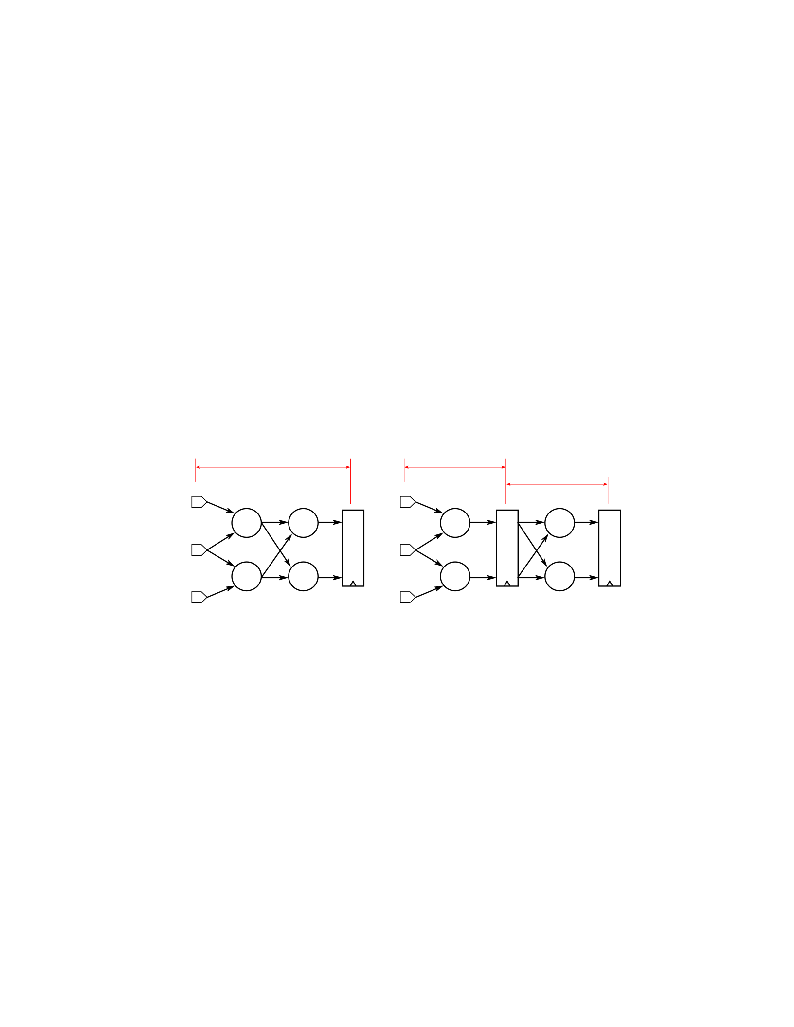
Figure 2.1: Pipelining simple feed-forward paths can lead to increased frequency at the cost
of extra latency. This is a relatively simple problem that has been addressed in commercial
tools.
then re-run implementation flow. Finally, the designer may discover new paths that need to
be pipelined – and the process repeats. This process is both time-consuming and error-prone.
In addition, it is not clear ahead of time how many extra stages will have to be added to the
design to reach the desired delay.
15
Comb
Logic
Comb
Logic
Comb
Logic
Comb
Logic
4 ns
Comb
Logic
Comb
Logic
Comb
Logic
Comb
Logic
ns2
ns2
(a) Original (b) Extra Pipeline

Automated tools for pipelining analysis in sequential circuits have been proposed in
commercial tools. Synopsys’ Design Compiler has the ability to insert extra pipeline stages,
balancing the timing in each stage [103]. However, this approach can only be used in simple
feed-forward pipelines, much like the example provided in Figure 2.1. Most modern designs
will contain pipeline branches, for instance multiple functional units in an FPU, or sequential
loops, like a forwarding unit in a CPU core.
A tool that is able to analyze the potential of adding more pipeline stages in more
complex designs has recently been introduced in Vivado [53]. Theoretically, pipeline stages
can be added in sequential paths in any design, provided that two conditions are met: 1) the
path is not included in any sequential loop in the design; 2) pipeline stages are added in
parallel paths to keep pipeline balance. In graph theory, a set of parallel paths in a graph is
usually called a graph “cut” and a minimum sized cut (min-cut) can be found through a
Maximum-Flow algorithm [60].
Another consequence of the conditions described above is that for any design, am
upper bound on the frequency that can be achieved is provided by the sequential loops in the
design. A simple strategy then is to find all paths in the design that are not in a sequential
loop and that have delay longer than the maximum delay within a loop. To minimize the
amount of registers added, a strategy like min-cut can be used, however, it is not strictly
necessary.
In practice, the presence of sequential loops is a major limiting factor. For a set of
around 90 commercial designs and IP blocks mapped to Xilinx FPGAs, it has been shown
that for around 50%, no improvement in frequency is possible due to the presence of loops
16

[53]. On the remaining 50% the improvement was of up to 6x, with 30 designs showing at
least 50% improvement on frequency [53].
In the remainder of this chapter, I discuss how Fluid Pipelines can further the
improvement in frequency by removing the constraint on sequential loops.
2.4 Fluid Pipelines
Elasticity is defined as functional correctness depending only on the order of events
and not the exact arrival time or clock cycle [27]. Events, also called tokens, are meaningful
data, from a designer perspective, flowing through a channel. A typical
Figure 2.2: The figure depicts the functionality of an elastic adder. Operands A and B may
arrive at different clock cycles and the latency may be arbitrary. Elastic Systems functionality
does not depend on the exact cycle events happen, but rather on their order.
execution example of a circuit implementing the elastic property is shown in Figure 2.2,
where the arrival of a valid token is represented by a number in a given cell. When a result is
produced, the token is consumed and can no longer be used. Empty cells in the table denote
that no new data has arrived in that cycle. Note that the latency between events is arbitrary3.
3 In practice, a circuit implementing elasticity will most likely be deterministic depending on the input set, but
this is not a formal requirement of the Elastic Systems specification.
17
Clock Cycle 6 127 81 9 102 113 4 5
A 0 4 3 7
B 1 2 5 6
A+B 61 8 13
To implement this behavior, Elastic System approaches have traditionally relied on
a pair of handshake signals signals: Valid (V) and Stop (S)4, which determine three states:
transfer (V = 1, S = 0), idle (V = 0) and retry (V = 1, S = 1) [41]. Fluid
Pipelines keep this convention, but could be built using other equivalent approaches.
The name Fluid Channel is used to denote a data bus and its associated control signals.
Towards this chapter, a Fluid Channel will be often represented as a single arrow for the sake
of cleanness.
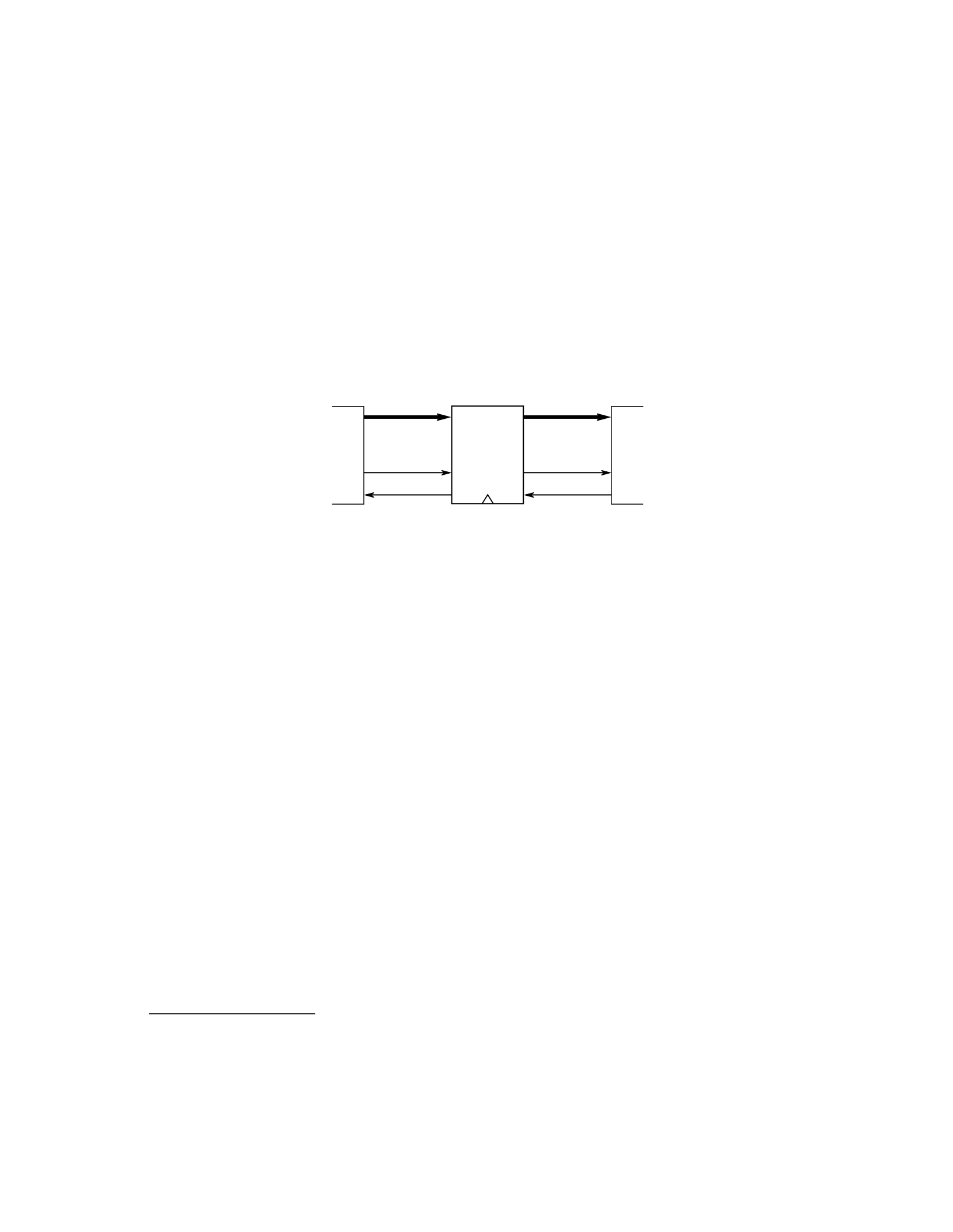
Figure 2.3: An elastic buffer is shown with respective sender and receiver sides, thick lines
denote multi-bit buses. An elastic buffer contains a data bus (din and q) and the valid (Vin,
Vout) and stop (Sin, Sout) handshake signals. Elastic buffers are the basic construct blocks of
Elastic Systems and can be viewed as queues with a limited size.
2.4.1 Communication and Flow Control
The inter-stage communication is performed through the help of Elastic Buffers
(EBs), storage units that replace registers, which include handshake signals both on the input
and output interface. Figure 2.3 shows the interface of an EB with input and output control
signals. Multiple implementations of EBs have been proposed in the literature (see [39] for
some). In this chapter, I do not discuss the trade-offs involved in each implementation, and
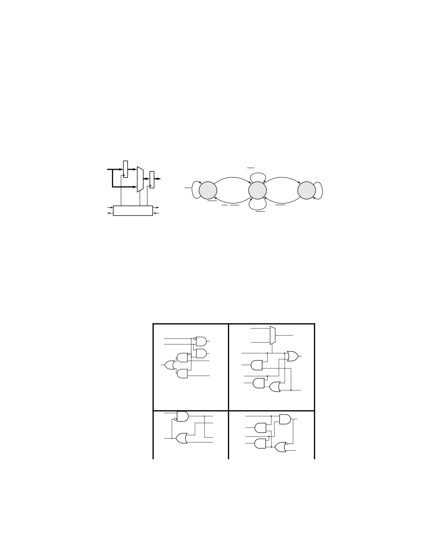
the experimental evaluation uses the implementation presented in Figure 2.4 that has
buffering capacity of 2, which has been used widely in prior work [41].
4 Other equivalent naming conventions have been used, e.g., Elasticity has been expressed in terms of FIFO
operation [104].
18
Sender
Receiver
EB
din
Vin
Sin
q
Vout
Sout
In general, each stage can have multiple input/output channels. To support this,
Fluid Pipelines rely on two pairs of control operators: one that maintains the ordering (Fork
and Join) and one that does not guarantee ordering (Branch and Merge). The basic
implementation of these operators is depicted in Figure 2.5. In Figure 2.5a, sel is a data-
dependent selection signal that indicates to which output the data will propagate. The
operators can be easily extended to more than two inputs/outputs.
(a) EB implementation (b) State diagram of Control block
Figure 2.4: The elastic buffer implementation assumed in this chapter is shown here, thick
lines denote multi-bit buses. (a) shows the datapath implementation with two registers, and
(b) shows the state diagram of the control block. This implementation works as a buffer of
size 2 with variable latency [41], but multiple implementations of elastic buffers have been
proposed [39].
1:N N:1
(a) Branch
Vi
VO1
SO
1
19
Control
Vin
din
Sin
Vout
q
Sout
c1 s c2
empty half full
Vin Vin.Sout/c1
Sout/c2
Vin.Sout/c2 /s,Vout,Sin
Sout
Vin.Sout/c1
/Vout
Vin
/c2,Vout
Vin.Sout/c2
Unordered
Vi
Si
VO1
SO1
VO2
SO2
sel
VI1
SI1
VI2
SI2
VO
SO
data I1
data I2
data O
(b) Merge
VI1
SI1
VI2
SI2
VO
SO
Ordered

Si VO2
SO2
(c) Fork (d) Join
Figure 2.5: The four operators used by Fluid Pipelines are shown in the figure for the 2 input
or 2 output versions. (a) shows the Branch operator which propagates data to one out of n
possible outputs, (b) shows the Merge operator that propagates data from any of the m inputs,
(c) shows the Fork operator that propagates data to all the n outputs, and (d) shows the Join
operator that propagates data when all the m inputs contain valid data. The operators translate
the intended functionality of a circuit and enable better design space exploration. Branch and
Merge are used when the relative order of operations can be broken, while Forks and Joins
enforce ordering. Note the difference in the handling of “valid” and “stop” signals.
Branch is used when the datapath forks into multiple paths, but data should
propagate to only one of them. This is controlled by the selection signal. For instance, an
operation in an FPU only needs to propagate to the appropriate functional unit, and the
selection signal is encoded by the operation bits. Merge operates as an arbiter: multiple
senders compete for a single channel. The sender that wins the arbitration propagates its data.
In the FPU example, a Merge would be used at the end of the functional units when results
from each unit are collected. Another way to think of the Merge is that it fires when at least
one of its inputs contains valid data. This is known as disjoint or-causality and introduces the
or-firing rule to the context of Fluid Pipelines. For simplicity and without loss of generality,
the proposed implementation in Figure 2.5b has simple fixed-priority, but can be replaced
with any of the existing elaborated arbitration schemes such as Round-Robin [86].
In general, Branch and Merge cannot be automatically inserted like Fork and Join,
because they alter the relative order between events. As a result, the programmer is
responsible for inserting them when needed. For example, in a complex Floating Point Unit,
just one Branch and Merge pair is needed after the normalization and denormalization stages
to indicate that the floating operations can complete out of order. On the other hand, the Fork
20

and Join operators can be automatically inserted in a similar way as the insertions performed
in traditional Elastic Systems. Branch and Merge can be performed with direct
Verilog/VHDL instantiation or just code annotations. To present, user annotations have been
used to determine which operators can be unoredered. More automated approaches, like
language support, are still open research questions that need to be addressed.
The use of special buffers and flow control operators are a source of possible
overheads in terms of area and delay. In particular, the mechanism to hold data when a stop
condition occurs requires buffering capacities as well as control logic, which could, in theory,
increase the area utilization needed by Fluid Pipelines. In practice, using simpler latches to
break down the buffering can mitigate the area impact and reduce the overhead to almost
none [102].
2.4.2 RePipe: Optimizing Fluid Pipelines circuits with ReCycling and
Retiming
As mentioned, Fluid Pipelines can be optimized by means of pipeline
transformations. Modern EDA tools perform operation such as gate sizing, time borrowing,
and logic replication to help improve timing and, hopefully, meet design specifications. All
those operations preserve cycle accuracy and can be applied to most synchronous circuits,
including Fluid Pipelines. The main advantage of Elastic Systems and Fluid Pipelines is the
ability to change the number of pipeline stages without breaking the system behavior.5
5 Note that inserting pipeline stages was proposed in synchronous circuits [53], but breaks the cycle accuracy
of the circuit and should be used with care.
21
To improve the frequency of Elastic Systems, it is possible to move EBs across
circuit blocks (Retiming) [25] (Figure 2.6a) or to insert additional stages in slower paths
(ReCycling) [25] (Figure 2.6b), ReCycling can also remove pipeline stages from noncritical
paths for power/area optimization. Retiming preserves the sequential behavior
(a) Retiming
(b) ReCycling
Figure 2.6: (a) Retiming is the operation of moving registers across combinational logic, it is
used to balance the pipeline, (b) ReCycling is the operation of changing, usually adding,
registers to the pipeline. Retiming and ReCycling are used to improve the circuit frequency,
but ReCycling decrease the throughput of Elastic Systems when applied to sequential loops.
of the circuit [25] and thus it can be applied mostly without penalties.
Inserting pipeline stages can be applied to Fluid Pipelines and prior Elastic System
approaches, but in prior approaches this comes with a reduction in throughput in cases where
pipeline stages are added to sequential loops. In fact, the throughput of the whole system is
limited by the loop with the lowest throughput, due to backpressure, even when this loop is
not used. The throughput of a cycle can increase with Early Evaluation depending on how
often each event occurs [66], but due to back pressure, there is still a limit on such mitigation.
Thus, in prior Elastic System approaches, ReCycling is able to reduce cycle time [53] but
may decrease the overall system performance in the case of stage insertion in sequential
loops [25,28,66].
22
F1 F2 F1 F2
F1 F2 F1 F2
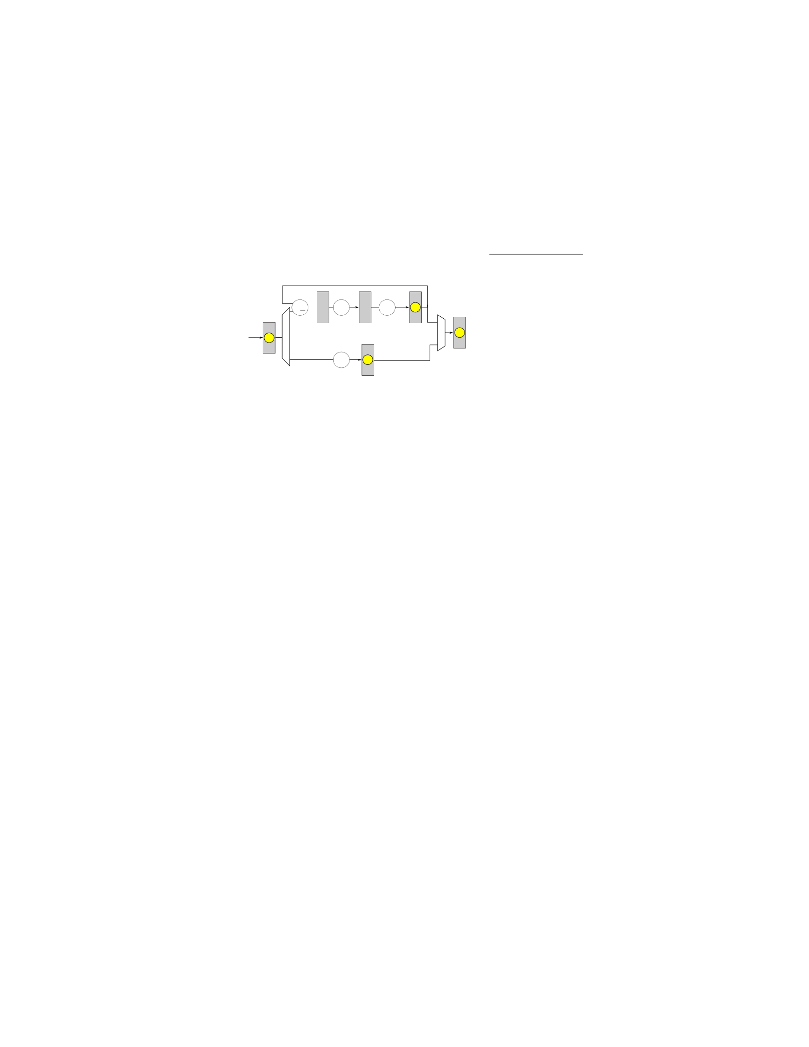
In Fluid Pipelines, on the other hand, unused paths are isolated from the remainder
of the circuit by the use of the unordered operators Branch and Merge. Since only used paths
are triggered when Branch and Merge are used, unused low-throughput paths do not
“contaminate” the overall system performance. This will become clearer
ID Path
Bottom Top
Bottom
Bottom Top
Bottom
Bottom
(a) Loop Case (b) Instructions
Figure 2.7: Toy case to illustrate the Elastic vs. Fluid approaches. (a) the test circuit, where
grey boxes indicate elastic buffers, circles represent combinational logic, and dots represent
registers with a valid token. (b) shows the instructions executed in this example and which
path they are assumed to use. in the next sub-section with a simple execution example.
2.4.2.1 Execution Example
To clarify the practical differences in the formalization between Fluid Pipelines and
prior Elastic Systems, let us analyze the sample execution in the example in Figure 2.7,
where circles represent combinational logic, boxes represent EBs, and the dots inside boxes
represent the presence of valid data (tokens). The paths are mutually exclusive (each
operation either takes the top or the bottom path), and the mux near the output EB chooses
23
in out
T1
F1
T2
F2
T3
F3
B
F4
I1
I2
I3
I4
I5
I6
I7

the appropriate path. The instructions can take either the bottom path or the top path in Figure
2.7b. The execution traces for traditional Elastic Systems and Fluid Pipelines are shown in
Table 2.1.
The execution order of Fluid Pipelines is altered (Table 2.1), note how in cycle 3, it
is possible to move I3 to the bottom path, while the top path is still executing. In the Elastic
System version, it is not possible to start I3, since the bottom path is shorter Table 2.1:
Sample trace for the toy case in Figure 2.7 considering both regular Elastic Systems and
Fluid Pipelines. Each line denotes a clock cycle and in which stage the instruction is at that
cycle. Fluid Pipelines improve throughput compared to Elastic Systems.
Elastic Fluid
Cycle in T1 T2 T3 B out in T1 T2 T3 B out
0 I1 I1
1 I2 I1 I2 I1
2 I3 I2 I1 I3 I2 I1
3 I3 I2 I4 I2 I3
4 I3 I2 I5 I2 I4 I3
5 I4 I3 I2 I6 I5 I2
6 I5 I4 I3 I6 I5 I6 I4
7 I6 I5 I4 I7 I5 I7 I6
8 I6 I5 I5
9 I6 I5 I7
10 I7 I6 I5
11 I7 I6
12 I7
and it would reach the output before I2. The re-ordering in Fluid Pipelines is a result of the
“or-firing” rule in the “in” stage and it is done because it was specified by the user, and not
24

changed by the tool. In a processor core, the reordering buffer performs this function, while
in network-on-chips, the reordering is usually not performed. Since this requirement is
application specific, it is left out of this dissertation. Here, it is assumed that any reordering
needed is performed in the design. In the case where order should be maintained, regular
Fork and Join operators must be used, causing the design to behave similarly to a Elastic
System.
2.4.3 Fluid Pipelines Deadlock Avoidance
One possible pitfall in Fluid Pipelines design is the possibility of deadlocks. Since
control is given to the designer, special care is needed when designing Fluid
Pipelines to avoid deadlock prone situations. Two properties are enough to guarantee that
Fluid Pipelines are deadlock free: No-Extraneous Dependencies (NED) and Self-Cleaning
(SC) [104]. Those properties can be summarized in the following design
directives:
•No-extraneous dependencies: If an output o of a module does not depend on an input
i of that module, then o should be produced regardless of the existence of valid data in
i. Also, the dependency list of o should be a subset of the inputs of the module.
•Self-cleaning: A circuit is self-cleaning if whenever it has produced n tokens in its
outputs, it has also consumed n tokens from its inputs.
These directives do not restrict which designs are possible, but rather how to
implement each design. To make it clearer why those properties are important and how the
25

directives work, let us take the example in Figure 2.8. The synchronous module described in
the figure has a pair of inputs (a and b) and outputs (c and d), c is a function of a and b, while
the value of d depends only on the value of b. Now, assume a designer wants to implement
that module using Fluid Pipelines.
The most straightforward implementation of the block would follow the behavior
described in Figure 2.9, where “xx_valid” and “xx_stop” denote respectively the valid and
stop bit for the “xx” bus. In this implementation, the circuit waits until all inputs have valid
data, and all outputs can accept new data to perform the operation. This is a violation to the
NED directive and can cause deadlocks depending on the context in which the block is used.
For instance, in cases where the output d is connected
Figure 2.8: Sample circuit to illustrate deadlock avoidance directives. The circuit contains 2
inputs (a and b) and 2 outputs (c and d) and performs two operations (f and g), one of which
(f) depends on both inputs and the other (g) depends only on input b. The handshake signals
are omitted for the sake of clarity. Fluid Pipelines design uses a few design practices to avoid
deadlocks. Those are restrictions on how to implement a given design and not on which
designs can be implemented.
1 2 3
4 5 6
7 8 9
10 11
12
26
f
a c
b d
g
always @ (posedge clk) begin
if (a_valid && b_valid) begin if(!
c_stop && !d_stop) begin
c <= f(a,b); d
<= g(b);
c_valid <=
true; d_valid
<= true; a_stop
<= false;
b_stop <=
false;
end
end
end

Figure 2.9: A pseudo-verilog snippet that generates a deadlock prone implementation of the
circuit in Figure 2.8. This implementation waits until all the inputs have valid data and that
all the outputs can receive new data.
as a feedback path to a, d will only produce output when both a and b are available.
A simple solution to this case is the use of a Fork operator (Figure 2.10). The Fork
operator isolates the handshake handling, and thus avoids the deadlock situation by avoiding
the unnecessary wait on a valid signal in a to propagate d.
The Self-Cleaning property is needed to avoid buffer overflow. Consider the case
where a circuit produces n inputs per token consumed. If there is a loop where the output of
the circuit is connected back to its input, there will be buffer overflow. For a
27

1 2 3
4 5 6
7 8 9
10 11
12 13
14 15
16
17 18
19 20
21 22
23 24
25 26
27 28
29 30
31 32
33 34
35 36
37
38 39
40 41
42 43
44 45
46 47
48
Figure 2.10: A pseudo-verilog implementation that solves the deadlock problem by using the
fork operator and thus avoiding the extraneous dependency of output d on input a. circuit
with buffering capacity of m, the overflow will occur after m/n cycles, causing a deadlock.
28
module fork(in, in_valid, in_stop, out1,
out1_valid, out1_stop, out2,
out2_valid, out2_stop);
//data input [N-1:0] in;
output [N-1:0] out1,
out2;
//handshake input in_valid, out1_stop,
out2_stop; output in_stop, out1_valid,
out2_valid;
wire ready = in_valid && !out1_stop && !
out2_stop; assign {out1, out1_valid} = {in,
ready}; assign {out2, out2_valid} = {in, ready};
assign in_stop = !ready;
endmodule
module f_and_g(a, a_valid, a_stop,
b, b_valid, b_stop,
c, c_valid, c_stop,
d, d_valid, d_stop,
clk);
//data
input [N-1:0] a, b;
output [N-1:0] c, d;
wire [N-1:0] b1, b2;
//handshake input a_valid, b_valid, c_stop,
d_stop; output a_stop, b_stop, c_valid,
d_valid; wire b1_valid, b1_stop, b2_valid,
b2_stop; input clk;
fork(b, b_valid, b_stop,
b1, b1_valid, b1_stop,
b2, b2_valid,
b2_stop);
always @ (posedge clk) begin
if (a_valid && b1_valid && !c_stop) begin
{c, c_valid, b1_stop} <= {b1, true, false};
end
if (b2_valid && !d_stop) begin
{d, d_valid, b2_stop} <= {b2, true, false};
end
end
endmodule

2.4.4 Fluid Pipelines Channel Grouping
In high performance design SoCs, it is common to have a guaranteed number of
cycles between events. For example, a cache hit in a processor may be known to take 3
cycles. The issue logic in the processor may start to wake up instructions two cycles ahead. If
the design shrinks/increases by 1 cycle, the time dependence may be broken. These scenarios
need to be taken into account in Fluid Pipelines, when adding extra pipeline stages. This
information is known by processor architects at design time and can be given to the Fluid
Pipelines framework.
To support this behavior, Fluid Pipelines allow the designer to assign group IDs to a
Fluid Channel. For simplicity, channels without user defined group ID are automatically
assigned a unique ID (i.e., empty group). When additional stages are inserted in a channel (or
existing stages are removed), all other channels with the same ID get the same amount of
extra stages. This guarantees that the relative number of cycles between the channels is kept.
There is no requirement that channels share wires or handshake signal and the number of
buffers already present in different channels do not need to match [86].
To illustrate this, let us analyze the example of an OoO core. Figure 2.11 shows the
instruction wake-up and data cache of an OoO core, the channels connecting wake-up to
execute and data cache to execute are assigned the same ID, and thus the
29
Issue Ex
D$
cID 1cID 1
cID 1
cID 1
a) Original(
Issue
D$
Ex
(b) Valid
Issue Ex
D$
(c) Invalid

Figure 2.11: The issue logic of a processor core is shown, arrows represent a data/handshake
bundle, shaded boxes represent elastic buffers and boxes with names represents pipeline
stages, the channel IDs is denoted with the arrows. (a) shows the original logic with two
cycles between issue and execute (Ex) units and one cycle between data cache (D$) and
execute, (b) an extra stage (shaded box) is added to both channels to create a valid pipeline
configuration, (c) a different number of stages is added to each path, yielding to an invalid
pipeline configuration. By annotating channel IDs, the designer can constraint what pipeline
configurations are allowed to guarantee the functional behavior of the circuit, this is specially
useful when there is dependency in the latency between two channels.
same number of stages need to be added/removed to them. A valid solution is shown in
Figure 2.11b, where one extra stage is added (shaded). The circuit in Figure 2.11c is not a
valid solution, since different number of stages is added in each channel.
An implication of channel grouping is that it is always possible to add pipeline
stages, but not always possible to remove pipeline stages in some cases. Figure 2.12 shows
two channel groups, out of a fully connected design graph (not represented for cleanness).
Group A has the same delay between producers and consumers. This means that any number
of stages can be inserted/removed in channels A1 and A2, as long as the number is the same
in both channels. Group B has similar constraint, but channel B2 has a number of stages that
is larger by one than channel B1. Strictly speaking, this means that pipeline B2 has to have at
least one pipeline stage. The minimum number
30
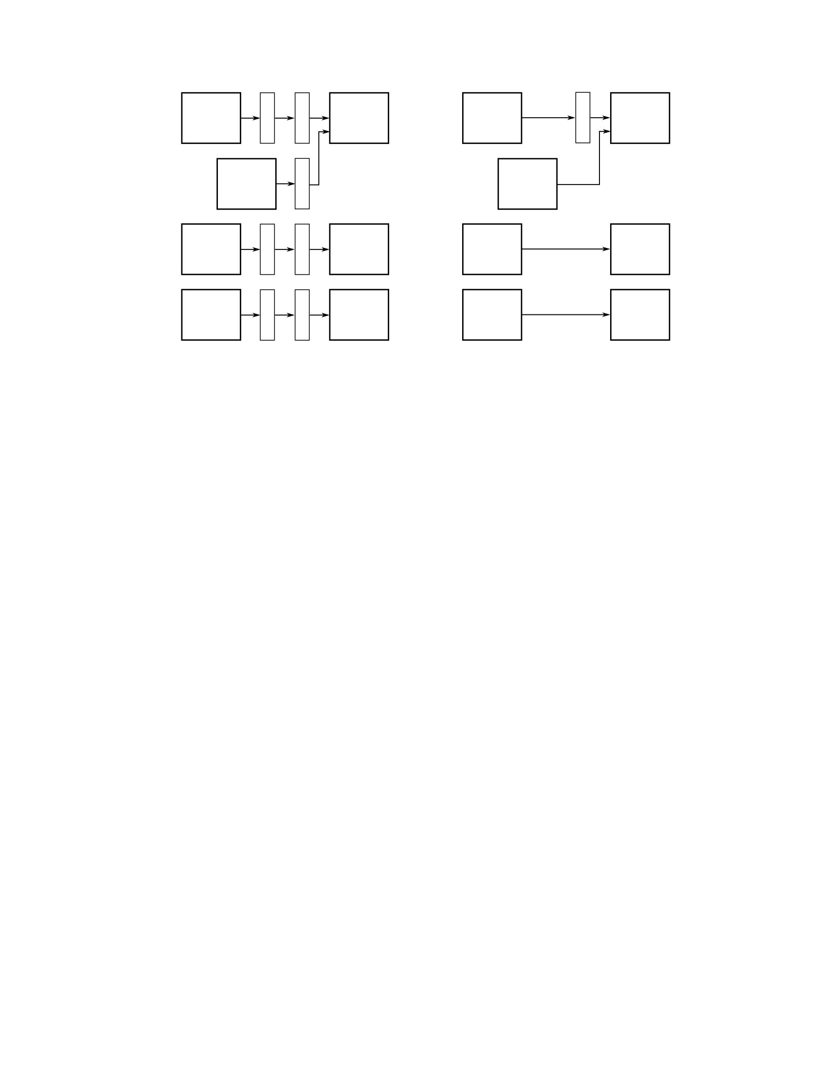
(a) Original Grouping (b) Minimum Stage Configuration
Figure 2.12: (a) shows 2 channel groups A and B. Each channel in A has two elastic buffers
(EB) between source and sink, whereas the channel B1 has one EB and B2 has 2 EBs
between source and sink; (b) shows the minimum pipeline configuration for both groups, for
group B it is not possible to remove all the EBs due to the uneven number of buffers in the
original configuration. It is not possible to remove all the stages in the design, but it is always
possible to add more stages. of stages in each case is shown in Figure 2.12b.
2.4.5 Design Example
Using Fluid Pipelines in dataflow is in general a straightforward task as seen so far.
In this section, I provide a different example of how memories or Register Files (RF) could
be integrated into Fluid Pipelines. When designing Fluid Pipelines it is common to replace
registers by EBs, but this is not desirable in the case of RFs, since RFs are supposed to hold a
value until a new value is written over it, and after reading from an EB, the data is consumed.
Instead, I show here how the memory abstraction (regardless of actual implementation) can
be used to model RFs, or any block of memory, in the RTL level.
31
EBEB
EB
EB EB
EBEB
Ch: A1
Gr: A
Ch: A2
Gr: A
Ch: B2
Gr: B
Ch: B1
Gr: B
EB
Ch: A1
Gr: A
Ch: A2
Gr: A
Ch: B2
Gr: B
Ch: B1
Gr: B

The idea is to create a wrapper over the memory block that implements the Fluid
Pipelines handshaking. Memory is represented as an array of registers, but a black-box
memory, from a memory compiler could be equally used. The Verilog code for the RF is
shown in Figure 2.13.
2.4.6 Design Overhead
One of the main disadvantages of Fluid Pipelines is the need for design intervention
in the RTL code. In this section, I look into how much of what is needed to implement Fluid
Pipelines already exists in digital design. In fact, finding points where Branch and Merge
operators can be inserted is a simple task because most existing
designs are inherently elastic.
Elasticity is omnipresent in digital design. Most designs already include signals
such as “start”, “done”, “busy” or “full”, which implement the logic used by Fluid Pipelines.
In some cases, like network routers, packages are well defined and routing/contention
schemes are already in place. That means that Fluid Pipelines does not require any logic that
may be unfamiliar to designers, but only standardizes how to implement this behavior.
To estimate what proportion of existing designs do implement the type of logic
required by Fluid Pipelines, I considered various designs in OpenCores,6 an opensource
database of digital designs. Even though those designs may not be an ideal
6 http://www.opencores.org.
32

module reg_file(in_data, in_addr, in_valid, in_stop, out1_addr,
out1_valid, out1_stop, out2_addr, out2_valid,
out2_stop, out1_data, out1_data_valid, out1_data_stop,
out2_data, out2_data_valid, out2_data_stop, clk); //addr and data
input [M-1:0] in_addr, out1_addr, out2_addr;
input [N-1:0] in_data;
output [N-1:0] out1_data, out2_data;
//handshake
input in_valid;
output in_stop;
input out1_addr_valid, out2_addr_valid;
output reg out1_addr_stop, out2_addr_stop;
output reg out1_data_valid, out2_data_valid;
input out1_data_stop, out2_data_stop;
input clk; assign in_stop = 0; //always
take inputs reg [N-1:0] registers
[REG_COUNT-1:0];
always @ (posedge clk) begin
if(out1_addr_valid && !out1_data_stop)
begin out1_data <= registers[out1_addr];
{out1_data_valid, out1_addr_stop} <= 2'b10;
end else if(out1_data_stop) begin
{out1_data_valid, out1_addr_stop} <= 2'b01;
end else
{out1_data_valid, out1_addr_stop} <= 2'b00;
if(out2_addr_valid && !out2_data_stop) begin
out2_data <= registers[out2_addr];
{out2_data_valid, out2_addr_stop} <= 2'b10;
end else if(out2_data_stop) begin
{out2_data_valid, out2_addr_stop} <= 2'b01;
end else
{out2_data_valid, out2_addr_stop} <= 2'b00;
if(in_valid) register[in_addr]
<= in_data;
end
endmodule
1 2 3 4 5 6 7 8 9
10 11 12 13 14 15 16 17 18 19 20 21 22 23 24 25 26 27 28 29 30 31 32 33 34 35 36 37 38 39 40 41 42 43 44 45
46
Figure 2.13: Sample Fluid Register File using register array in pseudo-Verilog. In this case, it
is simpler to keep registers as a memory block, instead of replacing them by EBs, so data is
kept after a read operation.
33

representation of practical/commercial designs, it provides a rich estimate from various
domains. Designs were classified as equivalent (same or inverted signals), partially
equivalent (only using one signal or using signals with different meanings), or nonequivalent
(not implementing any handshaking) to Fluid Pipelines handshaking mechanism. Only
projects marked as “DONE” were considered, in Verilog or VHDL and for which the code is
publicly available. Out of 270 projects, 35% are equivalent in most blocks, 10% are
equivalent in a few blocks, 20% are partially equivalent (in general, only “start” and “done”
signals). 25% implement no or an incompatible handshake. The remaining 10% are IO
operations (debouncer, LED control, …) or only combinational logic (lookup tables,
arithmetic operation, …).
These statistics show that the type of handshaking required by Fluid Pipelines is
already implemented in a significant number of designs, and therefore, Fluid Pipelines will
not introduce design overhead. The designer simply needs to annotate the code. It also show
that designer are used to the type of handshake used by Fluid Pipelines, and including them
will not be hard for any experienced designer.
Even though a large number of designs already contain some of the handshakes
proposed by Fluid Pipelines, there have been recent efforts to reduce the overhead of creating
new Fluid Pipelines designs. Liam [101] is a new paradigm for HDL that implicitly
implement Fluid Pipelines. Pyrope [100] is the first HDL to implement LIAM. Language
constructions like “consume” and “abort” are used to abstract behaviors typical of Fluid
Pipelines. Particular care is taken to avoid the construction of deadlock prone constructions. I
34

expect more languages to implement constructors that will ease the adoption of Fluid
Pipelines, however, this is out of the scope of this chapter.
2.5 New Evaluation Methodology
To find the optimal pipeline depth, a designer or tool must estimate the throughput
of a pipeline configuration (i.e., number and position of pipeline stages). In theory, this can
be accomplished through RTL simulation, cycle-accurate simulators or others. RTL
simulations are often slow, especially if a large number of configurations need to be tested.
For CPU cores, architects usually rely on standard cycle-accurate simulators, such as ESESC
[9]. Still, for other designs it may be hard to write custom simulators. Therefore, a more light-
weight methodology can be used to model simple designs faster and evaluate different
pipeline configurations early in the design time for space exploration, or late when changes
due to physical constraints are included.
A methodology based on Coloured Petri Nets (CPN) [62], a formal framework used
to model systems in different areas of computer science, was proposed to evaluate Fluid
Pipelines and other Elastic Systems alike [86]. The use of the coloured version of Petri Nets
is justified by the data-dependent Branch operations that cannot be modeled on the non-
coloured versions.
CPNs are defined as a bipartite graph of places and transitions, connected by arcs.
Places can contain tokens that have data value attached to them (colour). The state of the net
(the marking) is defined by the number and colour of tokens in each place. The initial
35

marking is changed when transitions fire. When a transition fires, tokens are subtracted from
its input places and added to its output places according to arc expressions. There is a
capacity associated with each place representing the maximum number of tokens in that
place, and prevents input transitions from firing.
Definition 1 A Coloured-Petri Net is a tuple CPN = ⟨P,T,A,Σ,C,G,E,I,Cap⟩:
•P is a finite set of places.
•T is a finite set of transitions, such that P ∩ T = ∅.
•A (⊆T × P) (∪P × T) is a set of directed arcs. Let a.p and a.t denote the place
and transition connected by a respectively.
• Σ is a finite set of non-empty colour sets.
•C : P → Σ is a colour set function which assigns a colour set to each function.
•G is a guard function that assigns to each transition t ∈T a guard function G(t) : ( ∅ ∪
Σ)|•t| → {0,1}, where •t = {p|(p,t) ∈A}.
•E is an arc expression function that assigns to each arc a ∈A an expression E(a), such
that the type of E(a) should match C(a.p).
36

•I is an initialization function that assigns to each place p ∈P an initialization
expression I(p), I(p) must evaluate to C(p).
•Cap : P → I is a capacity function that attributes a maximum capacity to each
place.
Firing Semantics: Let M, a marking function, map each place p ∈P into a set of
tokens M(p) ∈C(p). Let G(t)(M) (resp. E(a)(M)) denote the evaluation of G(t) (resp. E(a))
with the marking M. A transition t is enabled, and said to fire when G(t)(M) = true and ∀a ∈
{b|b = (p,t),p ∈P,b ∈A},E(a)(M) <= M(a.p), and ∀p ∈t•,M(p) < Cap(p), where t• = {p|(t,p)
∈A}. The firing updates the marking function to M′(p) = (M(p) E(p,t) ∪E(t,p)∀p ∈P.
Timing: In order to evaluate digital circuits, one needs to account for timing, which
is not included in CPN models. In regular CPNs, only one transaction fires at a given cycle.
Without changing the underlying semantics of CPNs, it is possible to change the model so
that every transition that is enabled at the beginning of the cycle fires. This is a more accurate
description of digital circuits and will help determine the number of clock cycles it takes to
execute.
There is one extra restriction to this formulation. The cardinality of each expression
must be 1; this means that for each arc, only one token can be consumed/generated. Also,
note that guard functions can only depend on the incoming arcs to a transition. This complies
with the constraints defined previously, and thus, avoids deadlocks. The restriction on the
37
cardinality of expressions changes the formalism of CPNs, and a formal analysis of the
impact of it needs to be further explored in future work.
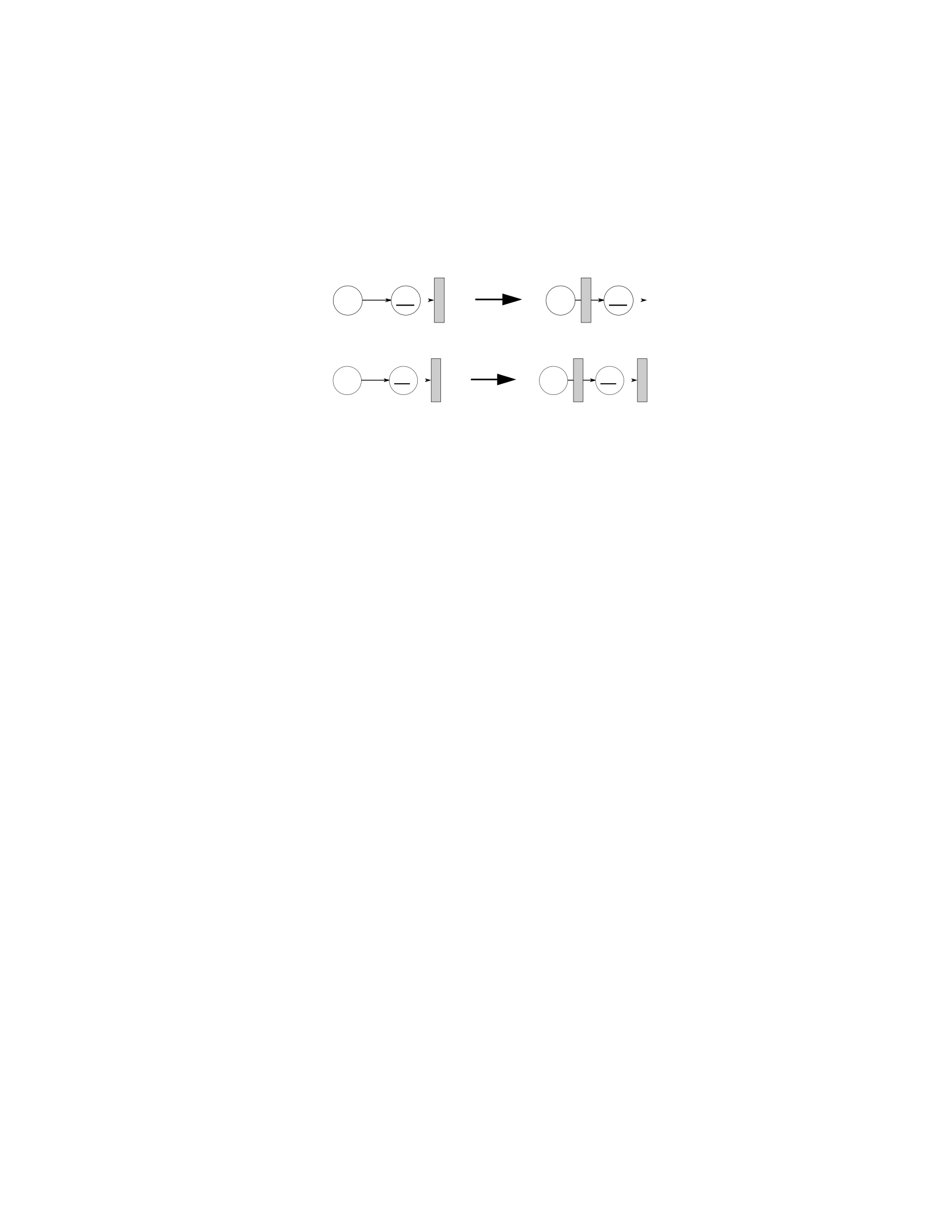
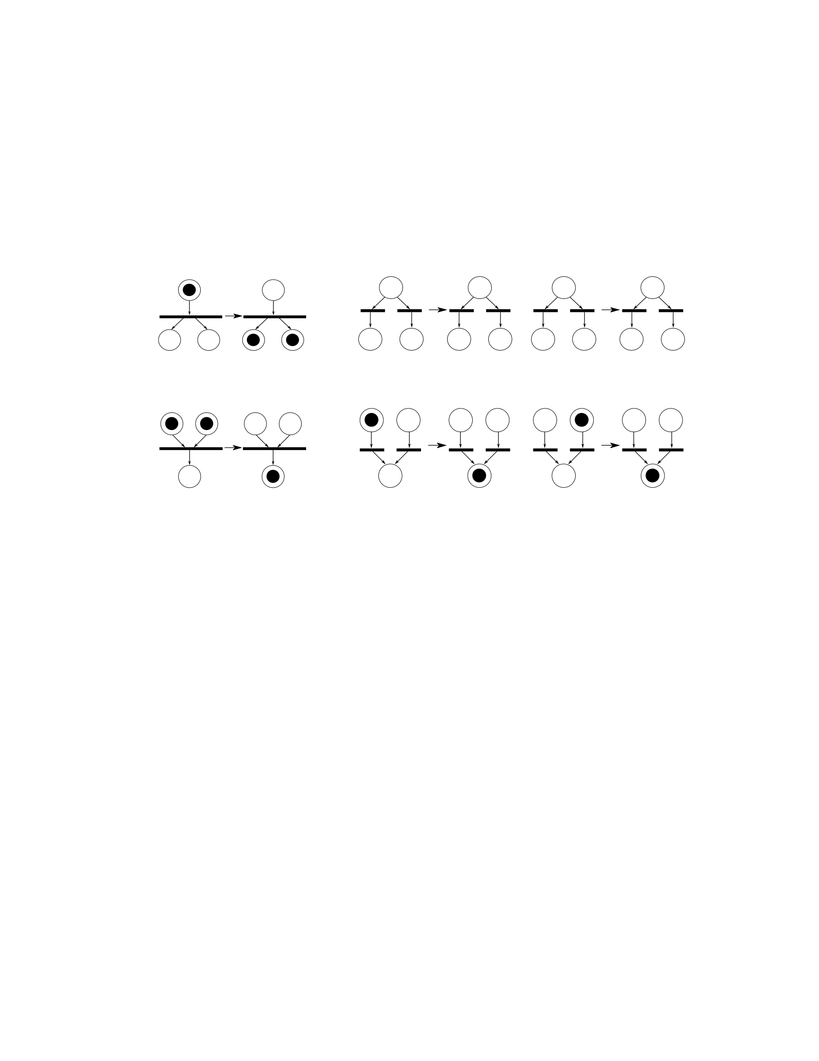
Figure 2.14 depicts how the Fluid Pipelines’ operators are modeled as CPN
transitions. Circles represent places, bars represent transitions, and dots represent tokens in
transitions that are not colour dependent while letters represent coloured tokens.
(a) Fork (b) Branch
(c) Join (d) Merge
Figure 2.14: The CPN models of each of the four operators used in Fluid Pipelines. The
models are shown before and after firing. Branch is data dependent and thus the arrows are
annotated with the expected data. Those models can be used to estimate the overall
throughput of Fluid Pipelines and Elastic Systems.
Merge operators do not define priority, and thus, conceptually both transitions can occur at
the same time, which is compatible with the theoretical formulation of Fluid Pipelines. While
places correspond to elastic buffers, transitions do not have a direct translation from the
circuit model. However, they can be mapped from the logic.
38
b
b
a
a
b
b
a
a
b
b
a
a
b
b
a
a
b
b
a
a

2.6 Evaluation
In this Section, I provide some experimental results that show how Fluid Pipelines
compare with prior Elastic System approaches, and what kind of trade-offs that Fluid
Pipelines enable. I first discuss the evaluation methodology and setup and then show the
experimental results.
2.6.1 Setup
A fully compliant IEEE-754 FP Unit developed by PhD students in my lab and a 2-
way Out-of-Order FabScalar core [31] are used to evaluate Fluid Pipelines [86]. They were
both designed as synchronous (for previous approaches), and annotated with Fluid Pipelines’
operators.
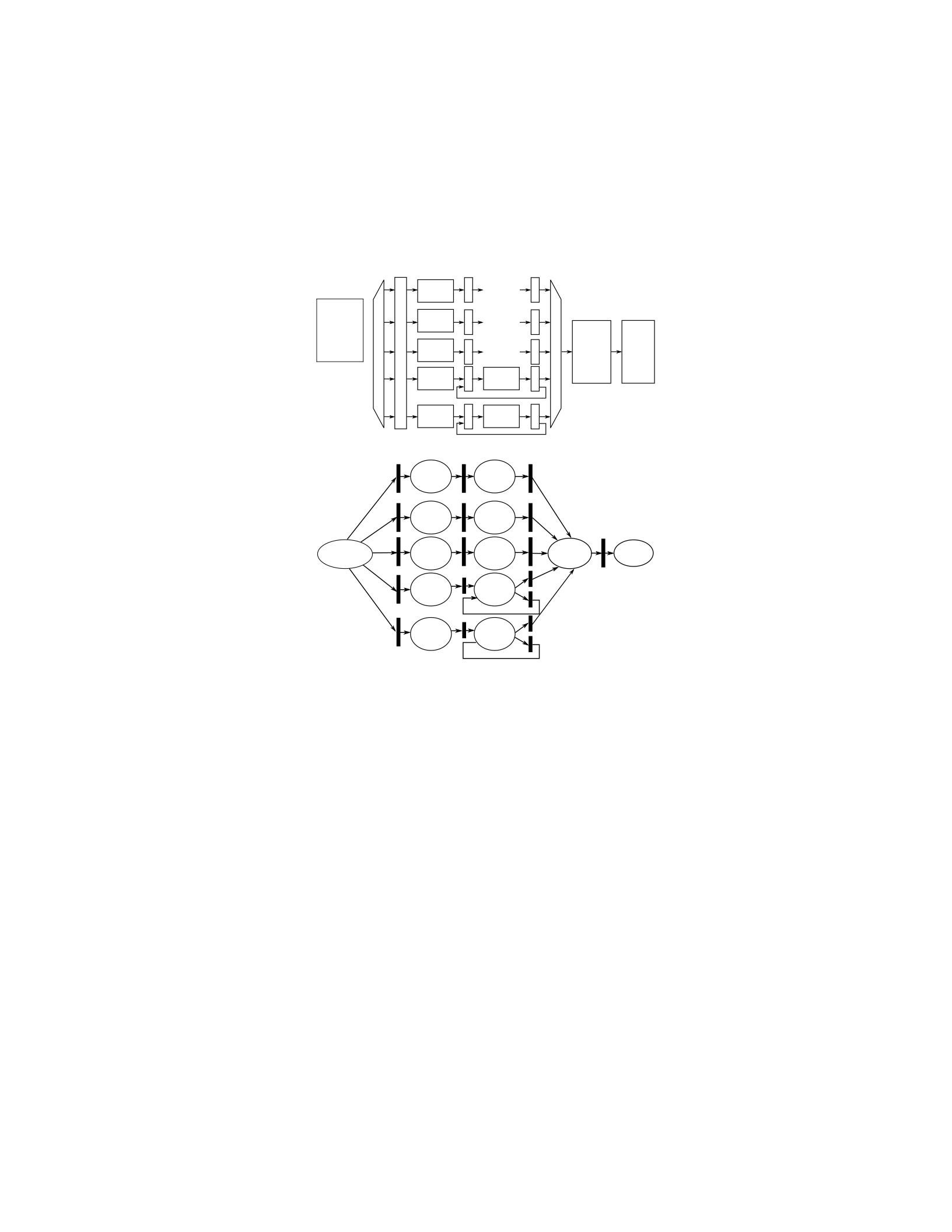
A functional block diagram of the FPU unit is presented in Figure 2.15a, and the
CPN model used for the performance evaluation considering Fluid Pipelines is shown in
Figure 2.15b. In this case, the Branch and Merge operators are used. Note how the division
and square root modules use the Merge to choose between the loop when the operation is
computing or sending the result to the queue when done. Both division and square root take
64 cycles to complete. For regular elastic, the Fork and Join operators are used instead.
The FabScalar-2W OoO core (Figure 2.16) contains nested loops and interactions
between blocks and allows us to explore the scalability of the different approaches.
Branch operators are used in the dispatch unit, exec units, bypass logic, and issue logic.
Merge operators are used after the exec units, bypass logic, in the free register pool handling
(ROB to Rename path), and in the next program counter calculation (Fetch
39
1).
Fluid Pipelines are compared against SELF [25,45] and LI-BDNs [104]. Elastic
Systems are implemented with EBs with storage capacity of 2. For LI-BDNs, queues of size
8 were used. In the SELF implementation adding pipeline stages to all the
denorm
(a) FPU
(b) CPN Model
Figure 2.15: The FPU block diagram (a) and the corresponding CPN model (b) used to
evaluate system performance.
40
add1
queue norm
sub1
mult1
div1
sqrt1
add2
sub2
mult2
div2
sqrt2
denorm
add1
queue norm
sub1
mult1
div1
sqrt1
a
b
m
d
q
add2
sub2
mult2
div2
sqrt2
d
d
c
c
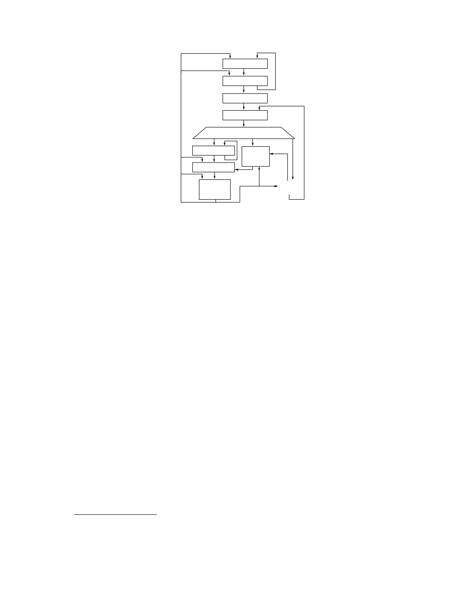
Figure 2.16: Block diagram of the FabScalar core used to evaluate Fluid Pipelines in this
chapter. An OoO core contains a complex structure of nested loops and interactions between
blocks. It is used to show the scalability of Fluid Pipelines.
paths that are parallel to the critical path will yield best performance and that is the
performance considered in this evaluation.
2.6.1.1 Benchmarks
For the FPU design, I report maximum and average throughput. Maximum
throughput is calculated by using a synthetic workload that only considers the best path (add,
subtract and multiply in this case). The average case is calculated as the throughput over a
million random instructions.
For the OoO core, only the average case over the SPEC2006 benchmarks7 is
reported. Per benchmarks results did not add much information and were therefore omitted.
2.6.1.2 ReCycling
7 Only the benchmarks that do not require Fortran were used.
41
Fetch 1
Fetch 2
Decode
Dispatch
Exec
Units
LS
Units
Rename
Issue
RF
ROB

The evaluation considers the addition of extra pipeline stages to each design.
Pipeline stages are added to the blocks with the worst delay. Perfect ReCycling/Retiming
(perfect balancing of delays) is assumed. Although this is usually not possible, this
approximation is sufficient. It is only necessary to ensure that after the insertion of a pipeline
stage, the two resulting stages have a delay smaller than the second most critical path before
insertion. Also, to account for register overhead, 2FO4 (fan-out-of-4) delay was added per
added stage.
To find the most critical pipeline stages, synthesis results for the FPU and previously
published data from FabScalar [31] that reports pipeline stage breakdowns were used. The
minimum pipeline configuration is the same as in the original non-elastic baseline: 6 for FPU
and 13 for the core.
Since ReCycling changes both throughput in instructions per cycle (IPC) and
timing, the performance metric used is throughput×frequency (equivalent to instruction per
seconds, IPS). Also, it has been shown that unless power is considered, the ideal pipeline for
a design is extremely deep [78]. Therefore, Energy Delay product (ED) is used. Power is
estimated from synthesis results for the FPU and ESESC [9] simulations (based on McPAT
[73]) for the core. Logic energy consumption (both dynamic and leakage) is assumed to
remain roughly constant independent of the number of pipeline stages. However, the dynamic
clock energy consumption increases linearly with both frequency and number of registers,
and the leakage clock energy increases linearly with the number of registers. This evaluation
does not consider the effects of Retiming, that may increase the number of registers added,
42

and assume that the added stages have roughly the same number of flops as existing ones,
which may not always be true in the case a stage is added in the middle of an operation.
2.6.2 Fluid Pipelines overheads
To evaluate the overhead of Fluid Pipelines, open-source RISC-V cores [13] of
various sizes and pipeline depths were re-implemented using Pyrope [100]. The cores were
synthesized using commercial tools and a commercial standard cell library. Even though the
comparison is not strictly fair, since those are still different implementations, it allows a good
estimate of how Fluid Pipelines compares with non-fluid circuits. The core compares were:
Zero-Riscy,8 a 2-stage core; VSCALE,9 a 3-stage core; PICORV32,10a 4-stage core; and
RI5CY.11 All the cores are 32 bits and the implementations in Pyrope were done over the
course of a quarter by another PhD student in my lab.
2.6.3 Results
I first show the design space exploration of the different approaches. In particular, I
show that Fluid Pipelines are able to push the Pareto frontier towards better performance and
energy efficiency. Then, I report the more detailed results, such as the maximum frequency,
throughput, and ED for different pipeline configurations for both the FPU (Section 2.6.4) and
Out-of-Order core (Section 2.6.5).
Fluid Pipelines push the design space towards more energy efficiency and better
performance. This is accomplished by avoiding false dependencies between concurrent paths.
8 https://github.com/pulp-platform/zero-riscy
9 https://github.com/ucb-bar/vscale
10 https://github.com/cliffordwolf/picorv32
11 https://github.com/pulp-platform/riscv
43
For most of the design points in the design space, Fluid Pipelines improve both better
performance and energy. In comparison, LI-BDNs reach better performance than SELF, but
at the cost of more energy (and area, not evaluated here).
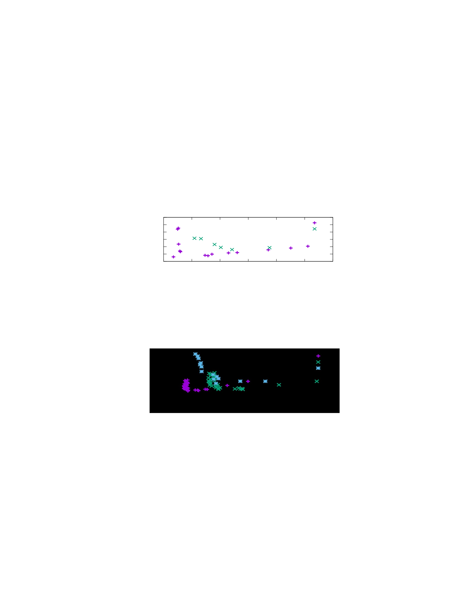
Near-Pareto frontier points (Figure 2.17) shows that for OoO core, Fluid
Pipelines (FP) deliver both less energy and more performance than SELF. Also, Fluid
Pipelines improve the best performance (by 6%, but with 28% less energy) and the best
energy point (by 14%, but with 16% more performance). Each point represents a dif-
Figure 2.17: Energy-delay curve for Fluid Pipelines and SELF for the OoO core. Each point
represents a different number of pipeline stages. The results show that Fluid Pipelines push
the Pareto frontier for the OoO core by improving both performance and energy.
Figure 2.18: Energy-delay curve for Fluid Pipelines, SELF and LI-BDN for the FPU design.
Each point represents a different number of pipeline stages. The results show that Fluid
Pipelines push the Pareto frontier for the FPU by improving both performance and energy.
44
0.6
0.7
0.8
0.9
1
1.1
1.2
0.6 0.65 0.7 0.75 0.8 0.85 0.9
Normalized Power
Normalized Delay
Fluid
SELF
Normalized Power

ferent pipeline configuration, where deeper pipelines tend to improve performance while
consuming more energy. In this case, LI-BDN was not used, as it will be explained in the
detailed evaluation.
For the FPU (Figure 2.18), LI-BDNs result in increased energy consumption due to
the increased storage, but improved the performance, when compared to SELF. Fluid
Pipelines present the best performance and energy out of the three schemes, since they do not
require extra storage. Compared to SELF, Fluid Pipelines improve the Table 2.2: The
maximum expected throughput with respect to the number of pipeline stages is shown for the
FPU design when using Fluid Pipelines, SELF and LI-BDNs. The original design contains 6
pipeline stages. Fluid Pipelines deliver constant maximum throughput, regardless of the
number of pipeline stages.
Pipeline stages Fluid Pipelines SELF LI-BDN
6 1 1 1
7 1 1 1
8 1 1 1
9 1 0.67 1
10 1 0.50 1
11 1 0.40 0.83
12 1 0 37 0.74
13 1 0.33 0.67
best performance by 120%, with 21% less energy, or improve the best energy by 12% with
230% improvement in performance. In comparison with LI-BDNs, Fluid Pipelines improved
the best performance by 33%, using 83% less energy, or improved the best energy by 38%
with 118% better performance.
45

2.6.4 Elastic FPU
The maximum throughput for each of the models is summarized in Table 2.2. Fluid
Pipelines deliver constant throughput regardless of the number of pipelines. The throughput
of SELF decreases when there is additional pipeline stages in the sequential loops. In the case
of LI-BDNs, the extra buffering helps maintaining the throughput even after the insertion of a
few stages in the loops, but after a certain number of insertions, there is back pressure due to
the dependencies.
The effective frequency, calculated for the average throughput, is reported in Figure
2.19. It does not necessarily increase with the number of pipeline stages. This is due the fact
that despite the frequency gain with the new pipeline stage, the reduced
Figure 2.19: The average throughput with respect to the number of pipeline stages in shown
for the FPU for Fluid Pipelines, SELF and LI-BDN. The average was calculated over a
random input set. In Fluid Pipelines, circuits can be ReCycled with higher throughput then
possible with Elastic Systems, and thus for better system performance.
throughput reverts the gains and reduces the overall performance. Since in the average case
the loop path is used, there is a reduction in the gap between Fluid Pipelines and the other
models. The same fact also causes reduction in the throughput of both SELF and LI-BDN.
Despite the reduction in the gap, Fluid Pipelines are still able to deliver a considerably
46
0.4
0.8
1.2
1.6
2
2.4
6 9 12
Million Instructions
per Second (MIPS)
# of Pipeline Stages
Fluid-av SELF-av LI-BDN-av
improved performance compared to SELF (120%), and slightly improved performance
compared to LI-BDN (40%), but using less resources.
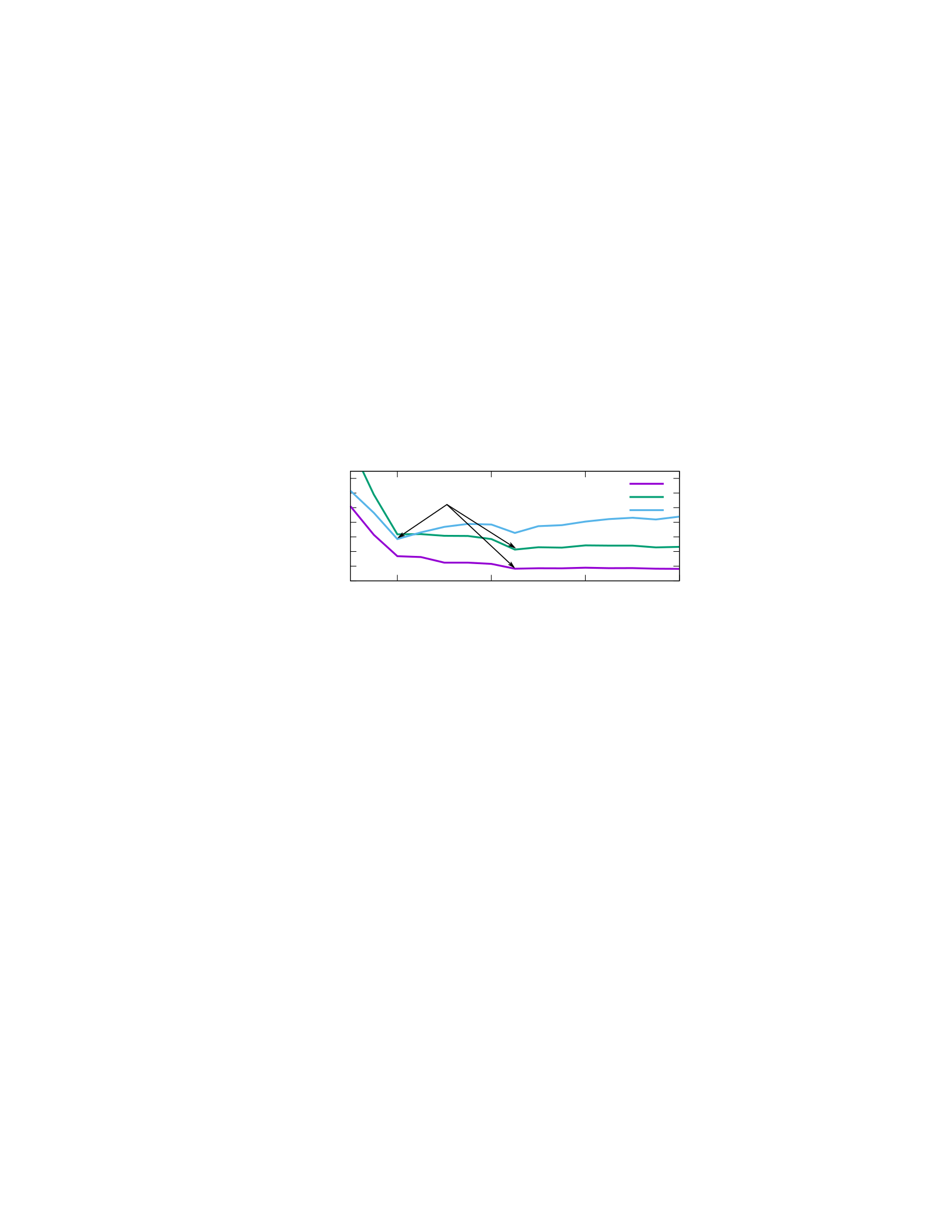
ED is reported in Figure 2.20. The energy overhead caused by the extra storage in
LI-BDNs reverses the advantages when compared to SELF. When comparing Fluid Pipelines
with SELF, Fluid Pipelines improve the best ED point by improving performance by 176%,
with 5% better energy. Alternatively, Fluid Pipelines deliver 120% better top performance
(with 21% less energy). When comparing Fluid Pipelines with LI-BDNs, Fluid Pipelines
improve the best ED point by improving both performance
(by 163%) and energy (by 25%).
1.4
1.2
1
0.8
0.6
0.4
0.2 0
Figure 2.20: Energy-delay product by frequency for the FPU design. The plot was made
varying the number of pipeline stages and calculating the ED product and expected frequency
for each pipeline configuration. Fluid Pipelines is shown to improve the best ED point of the
FPU, pushing the depth of the pipeline.
47
8 12 16 20
# of Pipeline Stages
Fluid
SELF
LI-BDN
Best ED
2.2 GHz GHz 4.2 GHz3.4 5.2 GHz
Normalized
Energy-Delay
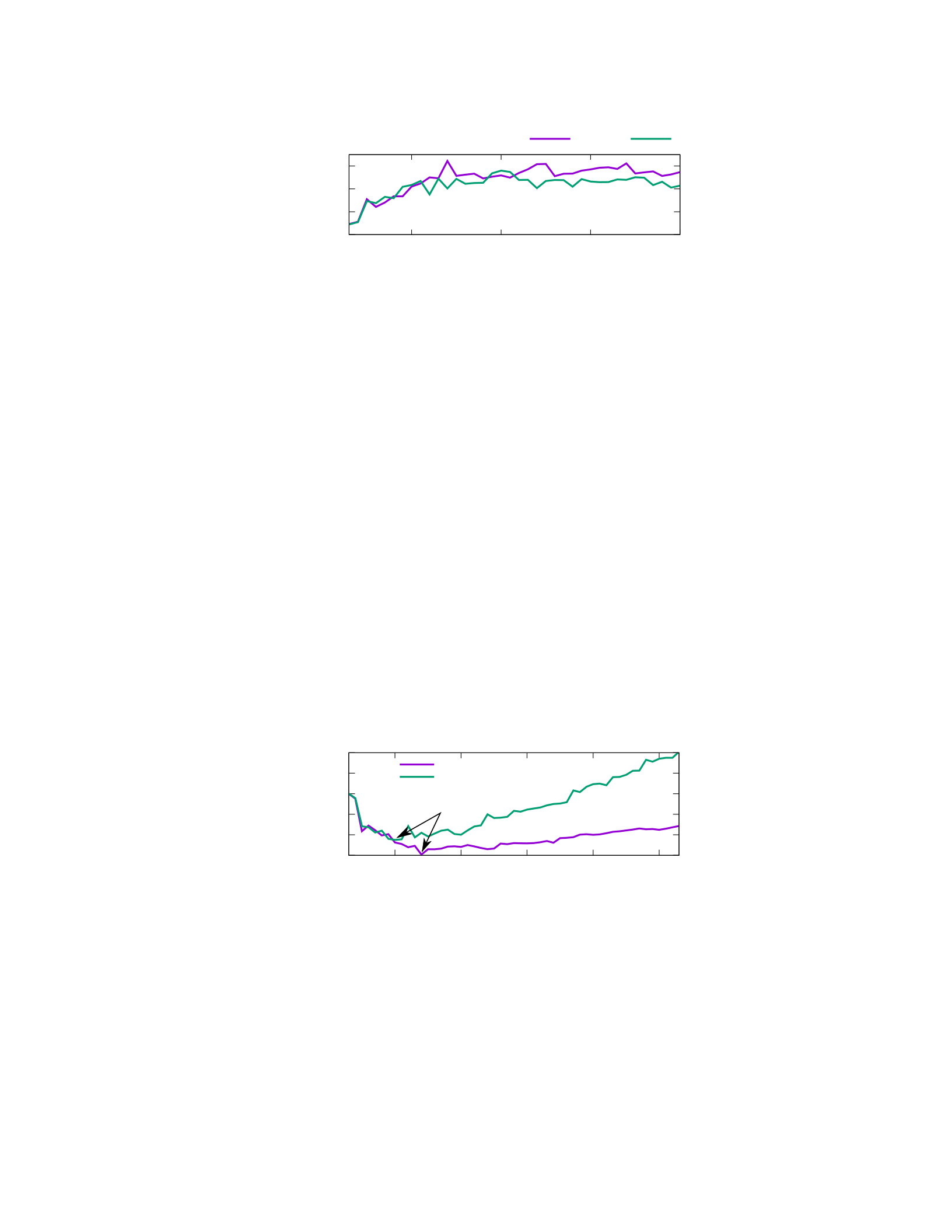
Figure 2.21: The plot shows effective frequency, in million instruction per seconds (MIPS)
for the OoO core. Effective frequency considers both throughput and frequency for each
pipeline configuration. Nevertheless, effective frequency alone is not a fair metric since it
does not consider the extra registers added by SELF.
2.6.5 Elastic OoO Core
LI-BDNs were not considered, since their main improvement over SELF is the
addition of FIFOs between modules. This is an important overhead for both area and power.
In addition, note from the previous experiment that for deep pipelining, LI-BDN behavior
approaches that of SELF.
As in the FPU case, the effective frequency fluctuates (Figure 2.21) when the
frequency improvement is not enough to compensate for the throughput decrease. Note
Figure 2.22: The energy-delay product is shown for each pipeline configuration for the OoO
core. The frequency shown in the x-axis was estimated based on the frequency for the
original design and the number of added stages. The figure shows that Fluid Pipelines shift
the optimal ED point of the pipeline depth and improve performance with a smaller power
overhead.
48
0.4
0.5
0.6
0.7
20 30 40 50
Million Instructions
per Second (MIPS)
# of Pipeline Stages
Fluid SELF
0.4
0.6
0.8
1
1.2
1.4
20 30 40 50 60
Normalized
Energy-Delay
# of Pipeline Stages
Fluid
SELF
Best ED
2.0 GHz 3.3 GHz GHz 5.3 GHz 6.4 GHz4.2

that for some points, SELF yields better overall performance than Fluid Pipelines. This is due
to the insertion of extra pipeline stages into all the paths that are parallel to the critical path,
which in some cases ends up hitting the second most critical path, and yields a better
frequency increase, with a cost in power and area (area is not reported).
The first few stages added increase the frequency considerably, with relatively
small hit on IPC (throughput) and energy. This leads to an improvement in the ED. As the
pipeline depth increases, the addition of extra stages has a smaller impact on frequency, but
lowers IPC more. In other terms, a relatively high number of stages (i.e., power overhead) is
needed to improve the overall performance, and thus ED gets worse. In SELF, when one
stage is added to a path, the optimal solution for throughput is to also add a stage in all
parallel paths with extra power overhead. Also in SELF, adding stages has a negative effect
on throughput. Combining these two effects results in a faster degradation of ED. Fluid
Pipelines shift the optimal number of pipeline stages, make a deeper pipeline configuration,
while improving energy by 13% and performance by 17%.
2.6.6 Evaluating the overhead of Fluid Pipelines
Table 2.3 shows the comparison between Fluid Pipelines cores and their nonFluid
Pipelines counterparts. PICORV32 is the smallest core, even though it is a 4-stage, and as
such, the Fluid Pipelines implementation is not able to closely match the original version in
size. For the 2 and 3 stages, area is very closely related between the Fluid Pipelines and non-
Fluid Pipelines versions.
49

There are some important differences both in area and delay, but it is worth noting
that the Fluid Pipelines cores were generated from a single code base with automated
transformations [102] and with very low effort over a small amount of time, whereas the non-
Fluid Pipelines cores come from different groups in a multi-year effort implementation in
some cases. For the open-source non-Fluid Pipelines version of the cores, it is important to
note that a lot of differences in the numbers come from differences in code style and not as
much from functionality or performance goals. In that sense, it is arguable that Fluid
Pipelines versions are within the noise level of differences in coding style and not really a
large constant overhead over non-Fluid Pipelines cores.
2.7 Conclusion
In this chapter, I discuss automated pipelining strategies, with a brief review of
repipelining techniques in non-elastic circuits and then presenting Fluid Pipelines, a new
abstraction for Elastic Systems. By using Fluid Pipelines, the designer has the Table 2.3: The
delay and area of 4 RISC-V cores are compared with Fluid Pipelines implementation of
similar cores. Fluid Pipelines shows low area overhead an similar delay to the non-Fluid
Pipelines counterparts. Delay data is normalized by the fastest core and area‘ data by the
smallest core.
Core Stages Non-Fluid Pipelines
Delay Area
Fluid Pipelines
Delay Area
Zero-riscy 2 1.78 1.20 1.73 1.29
VScale 3 1.60 1.00 1.73 1.61
PICORV32 4 1.00 1.76 1.31 1.78
RI5CY 4 2.18 3.67 1.38 2.00
50

opportunity to extract OoO execution from the circuit whenever possible, and boost the
design performance. Fluid Pipelines push the design’s Pareto frontier, by improving
performance and energy. In the experiments presented, Fluid Pipelines improve the optimal
ED configuration of an OoO core by improving energy 13% and performance by 17%, over
SELF. For a pure high performance configuration, Fluid Pipelines deliver 6% better top
performance while using 28% less energy. In addition, Fluid Pipelines brings the advantages
already existing in prior Elastic System approaches, like the possibility of changing the
number of pipeline stages, without breaking the design functionality, and thus improves the
ability of a designer to meet the design targets. The improvements brought by Fluid Pipelines
come from less throughput reduction where ordering was not needed but also due to the
ability of reducing the amount of buffering.
Fluid Pipelines can be used as a design strategy to generate multiple endproducts.
For instance, the same RTL can be used to generate a deep-pipelined high performance
design and a design with few pipeline stages for low power. It is common for companies to
keep multiple teams to create designs for each of those points. This practice leads to
replication of work and code, that could be easily avoided with a Fluid Pipelines-oriented
strategy.
I also present a modeling framework using Coloured Petri Nets, which allows
designers to evaluate the system runtime behavior, and perform early design space
exploration. This framework is later used to evaluate Fluid Pipelines against other Elastic
System approaches, showing an improvement in the overall throughput of the systems.
51

Fluid Pipelines open many research opportunities in EDA and architecture alike.
From a circuit designer perspective, Fluid Pipelines enable a more logic-oriented design
methodology, less worried with physical design constraints. For architects, Fluid Pipelines
provide a framework for flow control, opposed to the current token-credit approaches
commonly used in CPU cores. Fluid Pipelines also allow for faster exploration of the design
space and energy-delay trade-offs. But it is in EDA that Fluid Pipelines open the most
interesting opportunities. A number of automated transformations is possible in Fluid
Pipelines. I have discussed RePipelining (ReCycling + Retiming), but Fluid Pipelines
transformations are not limited to it. It is also possible to apply resource utilization techniques
of port sizing optimization and pipeline stage replication. For example, Fluid Pipelines allow
to increase or decrease the number of ports required by an SRAM without changing overall
system correctness. This is possible because when not enough ports are available at run-time,
it is legal to stall the inputs and wait until a free port becomes available. As long as the stall
operation is not frequent, the performance is not affected. Such transformation leverages the
handshake signals of Fluid Pipelines under the hood to generate the proper control signals.
A new hardware description language that incorporates Fluid Pipelines structures is
currently being developed [101]. It improves the ability to design circuits that implement
Fluid Pipelines directives abstracting away some of the lower level machinery needed. This
language has been shown to facilitate pipeline transformations and generate multiple design
points from a single RTL specification [102], and therefore automate the design space
exploration for multiple area-delay points.
52

Chapter 3
Anubis: A new benchmark for
incremental synthesis
A man who dares to waste one hour of
time has not discovered the value
of life.
Charles Darwin
In the previous chapter, I have discussed how automation tools can be used to
improve pipelining analysis and how Fluid Pipelines, a new paradigm for digital circuit
design, improves the opportunities for extra pipelining. While automating pipelining is an
important step for hardware design productivity, to get accurate estimations of frequency,
power and area for a circuit, a designers needs to perform synthesis. Runtime for synthesis
remains a major bottleneck for digital design, which this thesis proposes to address with the
use of incremental techniques. However, before I dive into incremental synthesis, I present
ANUBIS, a benchmark to evaluate incremental synthesis techniques. The lack of a
standardized benchmark that included designs and design changes is a gap and is one of the
main challenges for the creation of incremental synthesis.
53

3.1 Introduction
Synthesis and physical design (placement and routing) are tedious and time
consuming processes repeated multiple times during the design phase of a project [91].
Industry players have recognized this problem and have been trying to reduce synthesis time
by taking different approaches [6,107]. Nevertheless, the current standards are either limited
in results or require manual interactions, often increasing designer effort and degrading
Quality of Results (QoR).
Incremental synthesis techniques have been shown to improve synthesis time by re-
utilizing parts of the resulting circuit. These techniques have been applied in industry [6,108]
and in academia [30,91], but the lack of standard benchmarks makes it hard to compare
different approaches and to understand how the results presented in a paper can be translated
into “real-life” expectations.
Moreover, different approaches target different steps of the synthesis process,
making it harder to directly compare them, even if the benchmarks are the same. For
instance, the current version of Vivado includes incremental placement and routing [108] but
does not perform incremental logic synthesis, while existing research focus only on logic
synthesis [30,91].
There are multiple sets of standard benchmarks used by the design automation
community, e.g., the ISCAS benchmarks [23,24] or the ITC benchmarks [42] (among others).
However, these benchmarks do not target incremental flows. This prevents them from being
applied directly in incremental synthesis due to the lack of standard changes to those circuits.
Incremental synthesis benchmarks should be representative of real world designs, but they
54

should also include representative changes over which incremental synthesis is evaluated.
Moreover, when comparing multiple flows, the same set of changes needs to be used to allow
for a fair comparison.
Existing papers dealing with incremental synthesis have used ad-hoc benchmarks,
that included a variable number of designs, some of which may be “real-life,” but with rather
arbitrary changes. For instance, Chen and Singh [30] used 40 industrial benchmarks with
hand made “small” changes; while it is more likely that the designs come from actual
industrial applications, it is unclear whether the changes are reflective of real changes.
LiveSynth [91] used three publicly available designs and based their changes on commented
out code and repository history. This approach yields more reasonable changes, but the
designs used are not good representatives of industrial designs.
In this chapter, I discuss the first incremental synthesis benchmark suite, ANUBIS,
which includes a collection of open-source designs as well as standard changes. The use of
industrial benchmarks would certainly improve the representativeness of the benchmark set.
However, benchmarks should be made publicly available to ease adoption. Therefore, only
designs that are publicly available and can be freely used for academic research without
licensing are included in ANUBIS. On top of the designs used, ANUBIS introduces changes
based on repository history and commented out code, when available, with the addition of a
few synthetic changes that aim to exercise the case where RTL file changes do not result in
any logic change in the circuit (comments, variable renaming, so forth), as those could be
common and should not result in any effort by an “ideal” flow.
55

ANUBIS also defines a standard way of scoring and reporting results using
ANUBIS. The goal is to have an equivalent to the popular SPECint benchmark [56,63],
typically used to report performance numbers in CPUs. The unified ANUBIS score provides
an easy way to compare different proposals for incremental synthesis, while the standard
reporting requirements provides insights on where flows are doing a good or a poor job. The
ANUBIS score takes into account incremental synthesis time but also includes QoR results.
Finally, I evaluate ANUBIS using two commercial incremental synthesis flows over
ANUBIS. The results are reported in the proposed standard table with the final scores. The
evaluation shows that both the flows considered do a good job in delivering the same QoR
when in incremental mode, with a maximum of 4% of area degradation observed, and no
more than 1% increase in delay observed for both flows. However, the incremental synthesis
time is usually not proportional to the amount of changes. For instance, in cases where no
actual change was made, runtime was usually on the order of half of the full synthesis
runtime. More importantly for an evaluation of ANUBIS, the flow that has incremental
synthesis, scored better for the synthesis partial score, and the flow that has incremental
placement and routing scored better in those partial scores.
The main contributions of this chapter are:
• Propose ANUBIS, the first incremental synthesis benchmark set
• Propose a standard score and report table to facilitate the comparison of flows using
ANUBIS
56

• Evaluate ANUBIS using existing incremental synthesis flows
The remainder of this chapter is organized as follows. First, Section 3.2 presents
work related to incremental synthesis and benchmark construction for EDA. Then, in Section
3.3, I present the ANUBIS benchmark suite and some considerations on how to handle
different technology targets for synthesis, and in Section 3.4, I discuss the scoring function
for ANUBIS. The evaluation setup is described in Section 3.5 and the results are presented in
Section 3.6. I wrap-up this chapter in Section 3.7 with concluding remarks and discuss some
future steps for this research.
3.2 Related Work
The related work is split into two main parts: incremental synthesis techniques and
other benchmarks. In the first part, I discuss the type of work that could benefit from
ANUBIS and the benchmarks used in their evaluation. In the second part, I discuss how other
benchmarks (not necessarily for synthesis) work, how they were created, and how they are
evaluated.
Incremental Synthesis: The first incremental synthesis flow was proposed 30
years ago [64] in order to improve timing closure in digital design. The flow was interactive
and kept the design in memory while changes were being made by the designer. The flow
needed under 30 minutes to evaluate large (at the time) designs, but could compute the effects
in frequency of a small design change in only a few seconds. The main motivation of the
flow was timing analysis, with an incremental timer and the designer would manually
57

indicate design changes over the netlist to improve timing. There is close to no details on
what circuit was used in the evaluation or how changes were made.
Incremental synthesis was revisited more recently by other authors. Dehkordi et al.
[43] propose a flow that partitions the design into independent synthesis regions. After a
change is introduced only the affected partition is re-synthesized. Due to the artificial
partitioning method, there is a significant hit on QoR depending on the parameters chosen.
The authors used a set of 22 “industrial benchmarks” with manually added changes. There is
no information about the changes added, but it is clear that they were not based on real code
changes, since changes were “randomly” added. Benchmarks used were also not made public
due to their commercial nature.
To reduce the impact on QoR, newer approaches include detecting regions
impacted by the changes, regardless of an original partitioning of the design. A flow coupled
with Altera synthesis flows leverages information of nets whose functionality is not modified
during synthesis. When a change is made to the RTL, the flow maps that change to a specific
region defined by those “invariant” nets, replaces the synthesized of the affected region by
the elaborated netlist of the new code and launch synthesis over the design. Since most of the
design is already synthesized and optimized, there is little work that needs to be done,
reducing synthesis time [30]. A different approach is to only synthesize the modified logic,
which further reduces the synthesis time and has been shown to maintain QoR [91].
Incremental timing analyses have recently been pointed out to be a weakness in
timing-driven flows [58]. In modern digital design flows, timing analysis is essential to
identify critical paths and to avoid optimizing non-critical paths [69]. During performance-
58

driven optimization, timing analysis tools are used several times to assess the impact of
optimizations in the circuit [69]. Since most of these changes are localized, running full
timing analysis is a waste of resources. The recognition of this problem led to an academic
competition in 201512 for incremental timers. Although incremental timers are more geared
towards the optimization process of a static netlist, for instance, during placement, it is also
true that they could be used for incremental changes to the RTL, specially during the timing
closure loop.
Other Benchmarks: In the Incremental Timing contest the evaluation of designs
was done by using standard circuit benchmarks with changes generated randomly by a
computer program in the netlist level and not from real Engineering Change Order (ECO)
changes.2 The changes were described in the form of actions, such as “add/remove
connection”, “add/remove cell”, and so forth. Despite being useful to evaluate and test
incremental timing, those changes do not reflect real-world like changes that would be done
to a design.
The ISCAS benchmarks [23,24] are very popular in the synthesis and physical
design communities and have been used by countless research papers to evaluate and
compare different proposals. The ISCAS benchmarks consist of a set of netlists from real
industrial designs. Another set of benchmarks, the IWLS benchmark [4] include RTL
description of over 80 industrial designs, with the respective mapped netlists. The IWLS
benchmarks serve a more specific purpose for use in logic synthesis, but can also be used to
12 TAU 2015 Contest: Incremental Timing:
https://sites.google.com/site/taucontest2015/. 2Personal communication with contest
organizers.
59

evaluate parsers and elaboration tools. However, both these benchmark sets are static, in the
sense that they do not include changes that were made to those designs during their project
and therefore are not suitable for incremental synthesis evaluation.
Evaluating a benchmark is not an easy task. The most common problem associated
with creating and using a benchmark is to assess how representative it is of the expected
space of applications intended. For instance, on one hand excessive benchmark redundancy
was shown to be an issue due to the added runtime to evaluate the suite, on the other hand
reducing too much the number of entries in a benchmark can yield reduced coverage [84].
Another issue is to define which metrics are the most suited to evaluate a benchmark. For
instance, the placement community has been discussing between different metrics
(wirelength, routability, so forth) and the decision on which metric to use largely impacts
which placer will be considered the best [2]. A good benchmark should be able to rank
proposals according to well defined metrics, but in some cases, conflicting metrics make it
hard to intuitively determine which flow is in fact the best.
In the relatively new and largely unexplored field of incremental synthesis and
physical design methods, there is still need to define what it means to be the best, what
metrics are more relevant and how to weigh different metrics. In this chapter, I discuss some
of the metrics that I believe will be important and use them to compose a scoring system that
was used to evaluate existing commercial flows.
60

3.3 ANUBIS
ANUBIS, A New Benchmark for Incremental Synthesis, is a benchmark suite that
considers incremental changes in digital designs. The main premise of ANUBIS is that most
of the time during the design cycle of digital circuits, small and localized changes are
introduced to the code. Still, current benchmarks for synthesis (logical and physical) consider
mostly static benchmarks. ANUBIS tries to capture real changes that were introduced into
real designs. With ANUBIS, researchers working on incremental synthesis, placement,
routing, timing, bug finding techniques or others are provided with a standard tool to
compare their work more fairly and consistently.
ANUBIS consists of a collection of Verilog designs. The benchmarks were chosen
based on open-source status, availability of design changes (as explained later) and
size/diversity. ANUBIS was built trying to maximize the number and type of designs and
changes to be representative of a large set of real-life cases. In the next subsections, I
describe how the benchmarks were selected, how changes were inserted into the benchmarks,
and how to run ANUBIS to compare multiple incremental synthesis flows.
3.3.1 Benchmark Selection
The main objective of the benchmark selection criteria is to allow for a good
number of designs that are as reflective of real world designs as possible and have enough
real code changes in them. These criteria are not very strict, but work mostly as a set
of guidelines.
61

Closed source designs or code with limited distribution were excluded to prevent
limiting broad adoption. There is also a particular interest in looking for code changes. This
can take two forms: commented out code or repository commits. Given those two
requirements, the main source of benchmarks considered are open-source repositories online,
such as GitHub13 and OpenCores.14 The mipsFPGA softcore [55,61] was originally used in
one of my papers, but was finally not included in this benchmark set due to the restricted
distribution.
Another important source considered was from academic designs that were made
available with changes, for that research groups in multiple universities were contacted
directly. Designs from Bug Underground,15 a project at University of Michigan that aims to
find bugs in RTL code of cores, were added. They provide two processors with a large
number of bugs that are inspired into bugs found in commercial CPUs and reported through
erratas. Although those are not actual changes that were made to designs, they closely reflect
issues found in real commercial CPUs.
Generated code, such as from High-Level Synthesis (HLS), Bluespec, Chisel,
and so forth, were not considered. In theory, generated RTL could be used, but this adds an
extra layer to the benchmarks and is currently out of the scope of the benchmark suite. Those
may be considered for a future version of ANUBIS, in particular designs implemented in
Chisel and for HLS tools. After gathering open-source design candidates, the number of code
changes that could be found for them was considered. The code was inspected for
commented out code, and the commits in the repository for meaningful changes. Open-source
13 http://github.org.
14 http://www.opencores.org.
15 http://bugs.eecs.umich.edu.
62

designs with no design changes, as is the case of most of the designs in OpenCores, were
excluded.
Other variables considered are the ability to fit the design in a large highend FPGA,
to allow for flows to place and route designs for FPGA and that the design should not require
specific vendors. For instance, some designs use IPs specific to Altera or Xilinx, which
prevents them from being ported to other back-ends. Unfortunately, this leaves a very limited
number of useful designs, but more designs will be added to ANUBIS as they are made
available.
The list of ANUBIS designs is provided in Table 3.1. In the remainder of this
dissertation, the benchmarks will be referred to using the acronym presented in the second
column of Table 3.1. ANUBIS will be provided under the BSD License 2.0, and results of
flows using ANUBIS will be published on the official ANUBIS repository
(http://github.com/masc-ucsc/anubis), some of the benchmarks are distributed
under different licenses. Anyone using ANUBIS can submit results, and a list of top
contenders will be available in the official repository.
Table 3.1: ANUBIS consists of a collection of open-source benchmarks and standard changes
applied to it. Lines of Code (LoC), area and maximum frequency (Fmax) (for an ASIC 32nm
library using a commercial flow) are included as estimates of the design complexity. The
FPU design was provided by the MASC-UCSC lab.
Descriptio
n
Acronym LoC FMax
(MHz)
Cells
DLX core
[20]
dx 743 77
0
7152
ALPHA
core [20]
al 1086 66
6
17558
IEEE 754
FPU
fp 4716 250
0
58149
mor1k
RISC core
mo 1501
2
250
0
62752
63

[80]
OR1200
RISC core
[81]
or 1943
7
130
0
32928
0
3.3.2 Change insertion
In order to emulate design changes, code changes were inserted to the benchmark
code. The changes can be activated or deactivated through define statements. Some synthetic
changes were added to exercise some cases that are interesting but did not appear in either of
the above, such as replacing a signal by a constant. A change can be single-line, multi-line, or
multi-file. Changes include changing conditions in if statements, changing logic to generate
data, including/removing ports on a module, and others.
The main source of code differences used was commits in public repositories. In
particular, commits in nearby dates were considered, since ANUBIS specifically targets small
changes in code. Commits that added entire modules or sub-systems were not considered.
The idea of using commits from repositories is to try to mimic “real-word” work. Commits of
large amounts of code usually reflect the changes over several days or weeks which is not
aligned with the incremental synthesis philosophy. Commented out code was used when
available, following a methodology similar to the one proposed in [37]. In addition, changes
that cause syntax errors were ignored, but there are no assumptions on functional correctness.
Changes needed to be parsed and synthesized by Yosys [105] in order to be considered.
A special case where no logic change is inserted was also considered. For instance,
adding/removing comments, white space, changing variable names, so forth. The rationale
behind this is to understand how good the system is at detecting these corner cases where no
re-synthesis is needed. Ideally, a good implementation should be able to detect that there was
64

no change and return in almost no time. In some cases, this will not happen and at least a part
of the flow will be triggered. Those changes were artificially created, but were inspired in
cases observed in repository diffs.
Changes are divided into three categories: NoChanges, LocalChanges,
GlobalChanges. NoChanges are changes that do not reflect any real change in the behavior of
a system–they can be adding whitespace, double inversions, changing the name of a variable,
or actual changes to unused parts of the circuit. The LocalChanges category includes changes
within a module, mostly single line changes, or very localized changes, such as changing the
conditions on an if-else if chain, changing the constant values, arithmetic operations, so forth.
Finally, GlobalChanges are changes that either affect multiple modules or a module that is
instantiated multiple times in the design. Although changes are either classified as
LocalChanges and GlobalChanges, it is not necessarily the case that the amount of reused
cells will be lower for GlobalChanges, since this is largely flow-dependent. Moreover,
researches may be interested in different types of changes depending on the specifics of the
work being done, since different types of techniques will behave differently in each category.
Table 3.2: Summary of changes inserted in the benchmarks with breakdown by category and
source: actual code changes including git and commented out code (A) and synthetic
(S).
Design Total NoChanges
A S
LocalChanges
A S
GlobalChanges
A S
dx 27 0 4 23 0 0 0
al 15 1 5 9 0 0 0
fp 37 0 7 12 14 2 2
mo 34 0 7 20 0 4 3
or 31 1 5 19 0 4 2
A summary with the number of changes added to each benchmark is given in Table
3.2, with breakdown by category and source (actual or synthetic). For dx and al, all changes
are considered actual changes. ANUBIS is largely composed of LocalChanges, since the idea
65

behind ANUBIS is to leverage small incremental steps, although some GlobalChanges are
expected. The percentage of LocalChanges versus GlobalChanges approximately reflects
observations from the repository histories, although no statistical analysis over the histories
was performed.
3.3.3 Setup requirements to report ANUBIS results
For the sake of fairness, ANUBIS assumes that researchers will abide to ethics
when reporting results. Nevertheless, I discuss some of the “minimum” expected setup
conditions for a fair reporting on ANUBIS.
Equality in number of cores and resources used: When running full synthesis,
setup and incremental synthesis the same number of cores and physical resources (memory,
IO and network bandwidth, so forth) should be available. The workload on the computers
running the flow should also be consistent, and if at all possible only the benchmarks should
be running. The server configuration should be disclosed as much as possible, but at least the
number and model of cores used and the available memory should be reported. Note that if,
for instance, the setup flow is single threaded, the incremental synthesis could be parallelized,
but the results should be reported with a single thread. This measure prevents a flow of
scoring artificially high due to higher parallelism, and although parallelism is embraced and
encouraged, they are not the main target of ANUBIS.
High effort flow: Flow options should be chosen to achieve the highest quality
circuit. In general, that means, maximum (or within 5%) achievable frequency. The 5% is to
allow for approximation to integer numbers and to avoid pushing the flow to extremes, which
66

could incur large optimization overheads, that end up creating a lot of unpredictability to
runtime. However, flow options like “retiming” can be used at the researcher discretion, but
those should be consistent between full and incremental flows and should be clearly
disclosed.
Multiple runs: To reduce the effects of runtime variability, ANUBIS should be run
at least 3 times and the average should be used. If too much variability is observed (i.e., the
runtime between different runs differs by more than 10%), 5 runs are recommended.
3.3.4 Technology target
There is an important impact of technology target for synthesis, placement, and
routing in the overall runtime and QoR. For fairness, when comparing results, flows will be
divided into FPGA and ASIC targets.
If divergence due to specific standard cell library or FPGA vendors are observed,
further categories may be specified or generic open-source technology files may be made
available with ANUBIS. This is not expected however, since the scoring system is taking into
account the full synthesis as well, thus effects of specific technology should be captured and
taken into account.
3.4 How to score ANUBIS
An important part of a benchmark is to have a fair way of comparing different
approaches and answer what does it mean to be the best approach. That can be broken down
67

into finding the metrics of interest for the problem at hand and giving a relative weight to
them.
For incremental synthesis, knowing the percentage of reuse (changed cells, moved
cells, wires that needed re-routing) is an initial potential metric of interest, but as it becomes
clear in the evaluation, those do not necessarily translate into saved runtime. At the end of the
day, designers doing incremental synthesis are interested in reducing runtime and keeping
quality of results. Runtime savings and QoR are easily accessible from running the full and
incremental flows, although it is hard to place an absolute importance between them. For
instance, it is intuitive to think that a designer would not use an incremental flow that saves
90% of runtime but at the cost of doubling the delay. On the other hand, an incremental flow
that offers 10% speedup with minimal QoR impact may not be appealing either. However, it
is not as simple to decide if a designer would use a flow that reduces runtime by half with,
say, 5% impact on delay. That may be acceptable in some cases, for instance if a final
optimization synthesis can be performed later to catch up on the QoR gap. In those corner
cases, it may be harder to decide which of two flows is better.
Given that, I believe that the ultimate metric for incremental synthesis should be
related to runtime speedup, that is, how much time the incremental flow under evaluation can
save compared to the full flow. However, the flow should be penalized if it degrades QoR by
a “too much”, of course how much penalty for how much degradation is an important point
of discussion.
Runtime comparisons should be as independent of the hardware in which a flow is
running as possible, therefore ANUBIS uses runtime normalized by that of of running a
68

standard flow, which serves as a baseline for assessing the hardware power. It is also
expected that any incremental flow will require a setup phase that consists at least of an
initial synthesis, but possibly additional processing steps such as the approach proposed in
[30], change the regular synthesis flow to keep track of information needed later and include
extra steps beyond synthesis to prepare for the incremental steps. The runtime of this setup
phase is also considered, but is weighted less, since it should not need to be run often.
The scoring system is such that higher scores indicate better flows. The score
system works as follows: first a sub-score is calculated for each change in each benchmark
and the baseline benchmark (i.e., no change case). Then a benchmark score is calculated
based on the sub-scores. Finally, a global ANUBIS value is calculated using the benchmark
scores. The ANUBIS value takes into account the time to perform synthesis, placement and
routing. To provide better insights on the speedup, the standard reporting also includes
breakdown for each phase, as will be discussed later in this chapter.
3.4.1 QoR penalty
One important point to consider is QoR degradation. When performing incremental
synthesis, it is possible that there will be degradation in QoR. This is not a deal-breaker in the
sense that non-incremental synthesis may be used to close the QoR gap. Prior works on
incremental synthesis recommend running non-incremental synthesis while no changes are
being performed on the design [91]. Therefore, although it is important that a flow can
achieve accurate QoR, it is possible to tolerate small losses. However, if the losses are
significant, it may be impractical to use the flow. The scoring system takes that into account.
69

The answer to the question of how much QoR degradation can be tolerated may
vary significantly from case to case and from personal taste. Still, ANUBIS tries to capture in
general terms what may be acceptable in general to most designers and in most use-cases.
Since a hard consensus on a specific number would not be possible, I try to argue here in
more general terms. The first observation is that commercial FPGAs are divided into
speedgrade due to process variation. For instance, in Xilinx FPGAs the difference in speed
between grades is of about 14 − 15% [106], which indicates that
10% is too large of a variation to be tolerated. Another insight is taken from industrial blogs:
for instance, setting different clock constraints around the maximum achievable frequency
can led to Fmax differences of around 14% [99], which also seems to point that 14% is too
high. Another industrial post suggests that there is a variation of around 4 − 5% in
performance due to sign-off [79], which may seem to suggest that 5% could be a tolerable
error for most designers.
As a final argument, when 50 synthesis runs using Quartus over the same
unmodified design, there was fluctuation of, on average, around 3% in frequency [89]. This is
due to randomness present in the flow.16 The range was of about ±7%. This result also seems
to confirm that variability should be around 5% to be tolerable by designers. Therefore, ≈ 5%
QoR variation seems to be acceptable fluctuation, but ≈ 10% seems to be too much.
However, since there is not a definitive answer to this question, instead of using a step
16 Modern synthesis flows have been moving away from randomness for the sake of repeatability.
70

function, i.e., penalize any difference higher than 5%, ANUBIS uses a sharp but continuous
increase in penalty as QoR degrades.
The other piece missing to this discussion is how much penalty should be attributed
to flows that “break” QoR. The reasoning behind this is much simpler. If an incremental flow
is degrading QoR, it is natural to run the full flow to recover the penalty. Therefore, the
scoring function should be such that if QoR is within 5% of the full synthesis QoR, the score
is inversely proportional to the incremental synthesis time, and if the QoR is degraded to
unreasonable levels, the score is inversely proportional to the incremental synthesis plus the
full synthesis time, remember that higher scores mean better flows. This is called the
corrected runtime for change n of benchmark a: τ(an), where a is one of the ANUBIS
benchmarks and 1 ≤ n ≤ na is the change id and na is the number of changes for benchmark a.
Given that, the corrected runtime is given by:
tf(an)
τ(an) = ti(an) + (1 + α) × α + eβ×Qf(an)/Qi(an)(3.1)
where α and β are constants, ti(an) is the time it takes to run the incremental flow on change i
of the benchmark a, tf(an) is the time it takes to run the non-incremental flow on that
change/benchmark, Qi(an) and Qi(an) are the QoR metric of interest (critical path delay, area
or power) for the incremental and full synthesis flows respectively.
The constants were selected empirically, to have steep sigmoid function between 5
− 10% degradation in QoR, with 5% close to no penalty, high penalty for 10%, and close to
maximum penalty over 15%. The constants chosen were α = 108 and β = 26. There is no
71
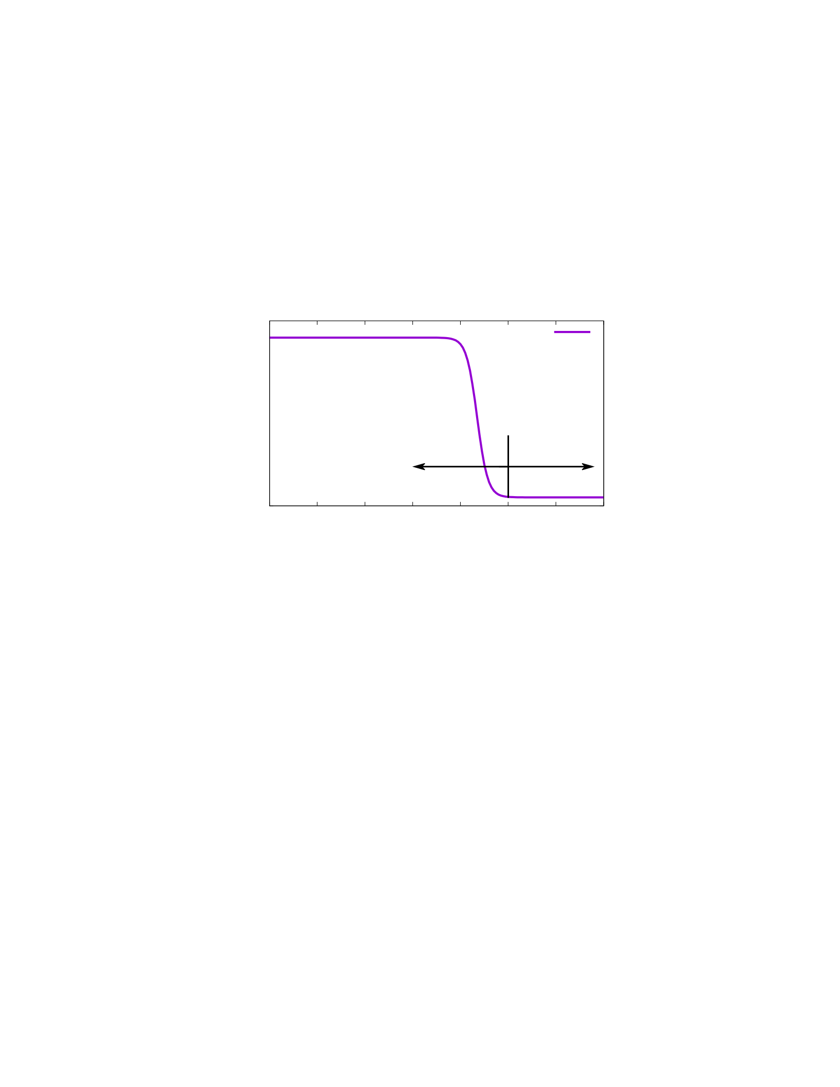
benefit for improving QoR. Figure 3.1 illustrates how this works, the x-axis shows the
percentage QoR change of the incremental flow compared to the full synthesis flow (100% is
the same QoR, and lower than 100% indicates degradation). The penalty rises sharply after
around 5% degradation in QoR up to the time it takes to perform full synthesis. Note that this
plot denotes the corrected runtime (τ) of the flow for change i of benchmark a, and therefore
higher is worse. This number will still be inverted before calculating the final score.
Figure 3.1: ANUBIS penalizes QoR loses. The penalty is dependent on how much QoR was
lost and on the full synthesis time. The rationale is that, if there is too much QoR degradation,
the full synthesis will be run to recover it.
3.4.2 Score
To make the score machine independent, i.e., to take into account that more
powerful machines would artificially improve the runtime, the score for each change in each
benchmark is normalized by the runtime of YOSYS (version 0.7+154) with a provided
synthesis script for that change in the same machine. YOSYS [105] is an opensource
synthesis tool that fully supports Verilog. The correct YOSYS version, the library for
techmap and the standard synthesis scripts are provided with ANUBIS, and will be run
72
00 20 40 60 80 100 120 140
Tau
Incremental QoR (%)
AN Score
QoR
degradation
QoR
improvement
tf + t i
ti

automatically. Changes to any of these are not allowed. The ANUBIS score an(an) for each
change is provided by:
tY (an)
an(an) = (3.2) τ(an)
where tY (an) is the YOSYS runtime for change n of benchmark a. This score is calTable 3.3:
Sample report table for ANUBIS.
Phase Delay Energy Area gmean Full
Synth ans,d ans,e ans,a gmean (ans)fulls
Place anp,d anp,e anp,a gmean (anp)fullp
Route anr,d anr,e anr,a gmean (anr)fullr
gmean gmean (and)gmean (ane)gmean (ana)gmean (gmean)gmean (full)
culated for synthesis, placement and routing independently, but since YOSYS only performs
synthesis the baseline is the same for the three. This is only to normalize for computation
power. One extra score an(a0) is added to each benchmark and is calculated considering the
setup phase of the algorithm. The idea is that longer setup times will result in a lower overall
score.
3.4.3 ANUBIS Value
For each phase (synthesis, placement and routing) and for each QoR metric (delay,
energy and area), the score an is calculated as the geometric mean (gmean) of all the scores.
This yields 9 values that are reported as a table (QoRs vs phase), and 6 sub-scores are
calculated as the gmean of rows and lines. The final of the flow ANUBIS score is calculated
as the gmean of the those. A sample standard report table is provided in Table 3.3. A set of
scripts to calculate the scores and generate the table is also provided with the benchmark
code. In each cell in the scoring table, a higher number indicates a better flow. Researchers
73

focusing on a specific phase can report a subset of the ANUBIS table and/or assume a
coupling with incremental approaches for other phases.
The table also includes a column with the scores for full synthesis flow. In this
case there is no QoR penalty, and thus there is only one column. The average speedup can be
obtained by dividing the gmean column by the Full column for each task. This already takes
into account any penalty in the incremental flow. Researchers working on specific areas may
want to add extra metrics. For instance, research in placement tools usually report routability
and congestion. This is also encouraged as it allows for better insights on trade-offs of each
tool.
3.5 Evaluation Setup
To evaluate ANUBIS, I rely on two commercial incremental synthesis flows (Flow
1 and Flow 2). There is little information publicly available about how these flows are
implemented, but the main focus of both flows is to reduce the impact on QoR while
leveraging as much as possible from the original design. For this evaluation, both the flows
are able to do incremental synthesis automatically, that is, without user intervention such as
user-defined partitioning and placement constraints, that are common in FPGA flows.
Incremental Flow 1 basically consists of regular elaboration and synthesis and
incremental placement and routing. Whenever a file is changed and saved, the regular
frontend flow is run over the design, and the incremental backend flow is ran over the
changes. Flow 2 also includes a frontend incremental flow that feeds the incremental backend
flow, and thus I would expect better scores in the first row of the ANUBIS for
74

Flow 2, in comparison with Flow 1 (higher scores are better).
ANUBIS is ran for the two flows independently, on a 32 core Intel Xeon E52689
with 64GB of memory, running ArchLinux-4.9.11-1. Timing measurement was done using
the tool provided time to avoid loading overheads. Delay, area and power were also used as
provided by the tool, post-routing. Each flow is run for each change in incremental and non-
incremental modes and QoR is compared for each change between the two.
3.6 Evaluation
In the first part of the evaluation, I show the standard ANUBIS table for both the
flows and discuss the results obtained. I also look into the behavior of each flow in the
NoChanges category, which provides an interesting sample use case to and could be a low-
hanging fruit to improve runtime in simple cases.
3.6.1 Overall Results
The results for Flow 1 are shown in Table 3.4. The best absolute scores are for
placement, even though routing is also supposedly incremental the tool still takes
considerable time in routing which explains the low scores. The results for synthesis are the
worst among the three phases, since it is not incremental. One good way to get insights about
the results is to look at the last column of the ANUBIS table that reports the scores for the full
synthesis flow. In an ideal case, with no QoR degradation, the speedup of the incremental
flow with regards to the full synthesis flow can be obtained by dividing the value in each the
gmean column by the value in the full column. In this Table 3.4: ANUBIS table for
incremental Flow 1.
75

Phase Delay Energy Area gmean Full
Synth 0.105 0.098 0.098 0.100 0.105
Place 2.982 2.704 2.704 2.794 0.175
Route 0.148 0.136 0.136 0.140 0.042
gmean 0.359 0.330 0.330 0.359 0.092
Table 3.5: ANUBIS table for incremental Flow 2.
Phase Delay Energy Area gmean Full
Synth 0.129 0.129 0.129 0.129 0.075
Place 0.039 0.039 0.039 0.039 0.039
Route 0.070 0.070 0.070 0.070 0.070
gmean 0.065 0.065 0.065 0.065 0.059
case, there is no speedup for synthesis, ≈ 15 times speedup in placement and ≈ 4 times
speedup for routing, on average.
The results for Flow 2 are shown in Table 3.5, they confirm the expectation of
better results for the synthesis phase when comparing with Flow 1. However, the results for
placement and routing are worse then Flow 1, which indicate that Flow 1 does a better job in
the incremental placement and routing then Flow 2. Overall, the much better placement times
for Flow 1 make it have a higher, and thus better, ANUBIS number. However, the Flow 2
scores for placement and routing are the same for incremental and full synthesis, which
indicate that the runtime for those phases are the same in both cases. This either indicates that
there is not really an incremental flow or that the incremental flow is a slow as the full flow.
Note that all the columns of Table 3.5 are basically the same. In fact, there was
actually some difference after the 5th decimal. This is because Flow 2 was very good at
preserving the QoR, with less than 1% differences between full and incremental flows. In
Flow 1, it is possible to observe differences mainly in the delay column, which has higher
numbers. The variation in delay for the Flow 1 flow was of up to 1%, but area and power had
76

differences of up to to 4%, which affects the score a bit. Since the median was of ≈ 1%, the
penalty is still pretty low.
One interesting note is that YOSYS took on average 8.83 seconds to complete
synthesis in the machine used. Thus it is possible to get average runtime, considering the
QoR penalty, for each task, multiplying the gmean column by the YOSYS runtime. Although
YOSYS is pretty fast for current standards, I believe that incremental synthesis should be
able to beat YOSYS. One evidence of that is the current score for placement in Flow 1.
3.6.2 No change cases
This section provides a sample use case on how to evaluate specific features of an
incremental flow. In this particular example, I look into how the incremental flows evaluated
behave in the case of NoChanges changes, i.e., simple code refactoring, such as comment
addition, variable name change, or whitespace addition. Intuitively, a smart incremental flow
should be able to detect that no logic change was made to the circuit, and no placement and
routing is needed.
Since the results for all the benchmarks were very similar, I will focus on the results
for fp. Figure 3.2 shows the runtime achieved by both flows for synthesis (Syn), placement
(Place) and routing (Route) when no actual changes are applied to the design.
In Flow 1, there is no change in synthesis compared to the full flow. For placement,
77

Figure 3.2: The flows tested cannot detect that no actual change was inserted and run at least
partially the incremental flows. Flow 1 does a very good job in placement presenting a
median runtime of zero for placement, but it does a poor job in synthesis and routing. Flow 2
presents a 2× speedup in synthesis, but placement and routing take a long time.
there is a reduction to zero most of the time. Routing is roughly half of the full flow. In Flow
2, the speedup observed for synthesis is basically flat in all the cases, and of around 2×, while
placement and routing have more varying runtimes, but in the order of up to 20%.
Although the NoChanges scenario is arguably less important, from this data it looks
like there is a lot of room for improvement in current incremental commercial flows. In
theory, it should be relatively easy to detect, at least after synthesis that no changes are
necessary in the physical implementation. This is an unexpected result, given that the reports
for both flows show that over 99% of cells and nets were reused from the original to the new
implementation. Thus, it looks like there is a lot of time spent in matching which cells and
nets can be reused, which eventually reduces the gains from the incremental synthesis.
78
0
50
100
150
200
250
300
Syn Place Route
Time (s)
Flow 1
Syn Place Route
Flow 2
Full synthesis

3.7 Conclusion
In this chapter, I presented ANUBIS, a set of RTL designs and code changes that
comprise the first benchmark set intended to be used for incremental synthesis, placement
and routing. In this initial version, ANUBIS is a small set of designs, but with a rich
collection of changes that represent real code changes applied to those designs during time.
ANUBIS considers both runtime and QoR to generate a final unified score that allows to
easily compare multiple flows.
Incremental synthesis has been the subject of various research in the past and has
gained traction in the industry as a path to reduce the synthesis time, which is recognized as
one of the main bottlenecks in digital design. Other research areas may also leverage
ANUBIS, such as incremental timing analysis tools.
ANUBIS was evaluated using two incremental commercial flows. Although there
are not many public available details on how those flows are implemented, they are more
focused on keeping QoR, since rather no QoR degradation was observed. This comes with a
cost in runtime, which was relatively high when considering the high reutilization of the
designs. Other approaches, such as LiveSynth [91], advocate for small QoR degradation for
more aggressive runtime reduction. In that case, the authors argue for the use of incremental
steps while the code is being changed, and full synthesis to recover QoR, when there is no
code change being performed.
As new benchmarks with code changes become available, they will be added to
future versions of ANUBIS, there is particular interest in larger designs that could help on the
study of the scalability of incremental flows and possibly reflect better industrial designs.
79

Generated RTL is also an interesting addition, since even small changes in the original code
can cause significant changes in multiple parts of a design. Finally, as new incremental tools
for synthesis emerge, the scoring system needs to be tested and validated against a larger set
of flows.
80

Chapter 4
Enabling Live Synthesis with
Incremental Methods
Rien n’est plus fort qu’une idée dont
l’heure est venue.
Victor Hugo
In Chapter 2, I described Fluid Pipelines, a new framework to enable adding and
removing pipeline stages at any point the during the design flow. While Fluid Pipelines
reduces the overhead of changing pipeline stages in a design, an accurate assessment of the
impacts of extra pipeline stages can only be obtained after synthesis, placement, and routing,
which remain costly. In this dissertation, I advocate for the adoption of incremental synthesis
as a way to mitigate this cost. Then, in Chapter 3, I presented ANUBIS, the first benchmark
to evaluate incremental synthesis that includes designs and code changes to them. In this
chapter, I discuss incremental synthesis that allows quick turnaround for synthesis and
evaluation of small code changes to a design.
81

4.1 Introduction
In the VLSI and FPGA design cycles, engineers typically wait several hours for
synthesis, placement, and routing. Most of the time, this is done for relatively small changes
while the design is being optimized, when the engineer is trying to assess the impact of a
single change in the overall circuit, often for timing closure. Incremental synthesis does not
exist in commercial ASIC flows, but it exists in commercial FPGA flows [6,107,108]. These
incremental passes try to cut the time to generate an FPGA bitstream; however, those
industrial flows are either not fast enough, as seen in Chapter 3, since they aim to guarantee
maximum Quality of Results (QoR) or rely on manual partitioning of the circuit, which often
degrades quality.
There is an important contrast of VLSI and FPGA design cycles with modern
software engineering techniques that advocate for agile development cycles [76], even with
live feedback for programming. While most software engineers would consider hours of
compilation unacceptable, this is the de-facto expectation in synthesis. I propose a different
workflow for hardware development that allow the designer to trigger synthesis results very
frequently as the design is being modified. Most of the time, providing accurate results takes
seconds instead of hours. This results in quick feedback to further optimize the design
without degrading quality. The proposed flow is an incremental synthesis flow on steroids.
Incremental synthesis is especially interesting for FPGAs on emulation platforms
like Strober [68] or FireSim [67], where short implementation time could reduce the
overheads involved in programming FPGAs during the evaluation of multiple similar RTLs,
82

with negligible QoR impacts. However, even for ASICs, synthesis flows could benefit from
faster feedback for evaluation of small changes.
Designers’ productivity should improve with an interactive synthesis environment,
as evidenced by the increase observed for agile software development [47]. My vision is of a
“live” flow, where designers know right away how the change will affect Quality of Results
(QoR). The flow is divided into two parts: an interactive, low-effort part, and a background
high-effort part. The interactive aspect gives “live” feedback
(within a few seconds) with good accuracy but not necessarily fully optimized designs. The
background process has a slow turnaround time and optimizes the design while the human
works in the next set of changes.
This flow allows more iterations per day, helping reduce the time for timing/power
closure. Since iterations are fast, the designer can make more changes, and thus it is easier to
track the impact of each change in the design. If the change did not positively impact QoR, it
is easy and cheap to undo the change and proceed in another direction. In this vision,
synthesis is triggered as the designer types or saves the file (as long as it is possible to parse
the code). This guarantees small enough increments while avoiding the undesirable old habits
of experienced designers that avoid triggering synthesis frequently. When there are no
pending incremental small jobs, a background high-effort synthesis runs to improve the
design quality. This background process aims to remove imperfections inserted by the live
flow, thereby slowly improving the design implementation.
To support this development model, in this chapter I present two distinct but
complementary ideas: LiveSynth and SMatch. LiveSynth is an incremental synthesis
83

framework that leverages an existing post-synthesis netlist to generate another postsynthesis
netlist for a small code change in the RTL of a design [91]. SMatch is a technique that
structurally compares two post-synthesis netlists to find structurally matching gates to re-use
placement and routing information, and thus reduce the amount of work the physical design
tool needs to do. There is no need for the logical function of the gates to match. SMatch can
theoretically be used in ASICs and FPGAs, however, since in ASICs gate sizes may differ,
SMatch is more suitable for FPGAs, where Look-Up Tables (LUTs) can be re-programmed to
implement any logic function.
In both cases, the target is 30 seconds of runtime. This target was set since 30
seconds is the time that the short-term memory lasts in humans.17 LiveSynth targets the front-
end flow, and can be applied to ASICs and FPGAs and even though SMatch targets the
reduction of placement and routing workload, it can be technically classified as part of the
front-end. Both the techniques are designed to be tool independent and can be adapted to any
synthesis, placement and routing flow.
Triggering synthesis over the whole design is widely adopted in industry and
academia alike. Nevertheless, usually, at a given iteration, a designer is focusing on one small
portion of the circuit. In traditional synthesis, even if a small portion of the design is changed,
logic synthesis and placement are triggered for large blocks and require hours to complete.
This is due to two main reasons: tools are not designed for incremental synthesis, and inter-
module optimization has a significant impact in QoR, which makes it hard to assess where
the impact of a change is important.
17 Personal communication with faculty in the Psychology Department at UCSC.
84

The techniques presented in this chapter focus on highly optimizing the subregion
and triggering re-synthesis only when necessary, and not over the whole design. LiveSynth
divides the design into multiple regions with invariant boundaries, i.e., regions whose
boundaries’ functionality has not been changed during synthesis. These regions are smaller
than user defined modules on average. When a change is made in the RTL description of the
design, the synthesis flow needs only to find which regions were touched and replace them
with the newly synthesized netlist. SMatch leverages existing placement and routing
information, which are known to be a good, if not somewhat optimal, implementation of the
circuit, and then only re-places and routes gates as needed.
Even though each region is highly optimized, this process is much faster since the
region that is touched by the flows is kept small. To be able to maintain QoR, especially
delay, if part of the critical path is within the region, the neighboring regions are also
included in the high effort synthesis. Special care is given to the case where multiple
instances of a module exist in the design. If the region frontiers are within the module, the
region can be optimized alone, which yields a faster process. In the case where the region
frontiers are outside the module, each instance must be dealt with
separately.
SMatch can operate over the whole design, and should still be relatively fast, since
to a structural comparison of the circuit can be done in linear time. However, LiveSynth can
be leveraged to reduce the search space. In any case, both techniques include a setup phase
that performs a regular synthesis of the whole design and also finds invariant regions, which
are used as incremental grains for the incremental phase. When there is a change in the RTL,
LiveSynth finds which regions were affected and synthesizes only them. The algorithms are
85

designed so that LiveSynth does not traverse the whole graph. Then if SMatch is used to find
structurally matching components and keep place and route information. Finally, the regular
place and route flow is used over the unmatched cells within the incremental synthesis
region.
The results showed that LiveSynth was able to reduce synthesis time by about 10×
on average, but with high variation. LiveSynth was consistently faster than any of the
previous approaches. When coupled with SMatch, the flow was able to deliver a fully placed
and routed design in about 16−20× faster than a regular flow, or 2× faster than LiveSynth, on
average. SMatch was able to finish synthesis placement and routing in less than 30 seconds
for 70% of the changes in the Anubis benchmark suite [89]. SMatch was faster than previous
approaches in most of the cases, but it was never slower. There was a slight degradation in
QoR but not statistically distinguishable than previous approaches, only a minority of design
changes had degradation and never more than 3% degradation in delay.
The main contributions presented in this chapter are:
•LiveSynth, the first incremental synthesis flow that allows inter-module optimization
• Interactive synthesis methodology with fast feedback
• Incremental synthesis flow that is independent of a specific synthesis tool
•SMatch, the first synthesis flow that leverages the structure of the netlist to reduce
placement and routing
86

• First proposal of SMatch, a flow that leverages the pre-fixed nature of FPGAs to
accelerate synthesis results
The remainder of this chapter is organized as follows. First, I discuss related work
on Section 4.2. Then, in Section 4.3, I present LiveSynth, which is the main building block for
this chapter. I discuss how SMatch builds upon LiveSynth in Section 4.4. Then, Section 4.5
discussed the evaluation setup and Section 4.6 the main results. I wrap-up this chapter on
Section 4.7.
4.2 Related Work
Incremental synthesis tools are by no means new. An interactive synthesis flow was
first proposed over 30 years ago [64], motivated to improve timing closure in digital design.
The authors claim that the flow needed under 30 minutes to evaluate relatively large designs
(for the time), but could compute the effects in frequency of a small design change in only a
few seconds of CPU time. Although the main motivation was timing analysis, the result is
largely an incremental (though manual) synthesis flow. The whole circuit is kept in memory
while the designer applies small changes to it.
Incremental flows also exist to target software compilation [97]. This technique
consists of identifying which functions are affected by a single code change and then only
recompiling those functions. Authors put particular effort into checking inline functions–code
that was declared a function by the programmer but was merged into its calling point–as well
as inter-procedural optimizations. Those are the main challenges in incremental compilation
87

and can be translated to inter-module optimization in RTL synthesis. The techniques used
here are sensitive to inter-module optimization.
Multiple incremental synthesis flows have been proposed. Early [43] and still
widely used [6] flows rely on pre-partition of the design, either manually or automatically.
Each partition is independently synthesized, placed, and routed, and then the overall circuit is
connected together. When changes are made, only the affected partitions are re-synthesized,
placed, and routed, reducing the total time. However, the QoR is heavily dependent on the
partitioning, and there does not seem to be a way of predicting which partitioning method is
the ideal short of trying multiple partitioning strategies.
Traditional ECO approaches [34, 77] can also be classified under the larger
umbrella of incremental synthesis, but the main goal of ECO flows is to reduce the amount of
disturbance to an existing mask, usually late in the design process where it is costly to change
the design. Therefore, the algorithms and methods used are well suited to reduce the amount
of cells changed, wire re-routed and so forth, and not necessarily to keep overall quality or
reduce runtime [21]. The approaches presented in this chapter do not look into minimizing
the size of changes as much, since they are focusing more on the timing closure cycle, which
is typically earlier in the design cycle than ECOs.
Finally, post-synthesis partitioning methods first synthesize the design and then find
suitable partitions. Because these methods do not arbitrarily decide where to partition before
synthesis, they have the advantage of minimizing QoR degradation. Both LiveSynth and
SMatch fall within this category. Line-Level Incremental Recompilation (LLIR) [30] propose
a line-level incremental synthesis flow that is implemented coupled with the Altera synthesis
88

flow. Since this flow has access to internals of the synthesis flow, it is able to keep track of
changes during the synthesis flow and reduces the setup overhead observed in this approach.
The final proposal also incurs in the elaboration of the whole design at each change and
launches the synthesis over the full design. The approaches discussed here are more efficient,
since they reduce the amount of work in the RTL elaboration, the final synthesis, and in
placement and routing. They also be used with different synthesis tools without accessing any
code.
4.3 LiveSynth
LiveSynth works by creating an implementation for a modified RTL specification,
utilizing as much as possible from a previous implementation for the original specification.
Incremental flows rely on partitioning the design into regions that will be independently
synthesized. Then, re-synthesis can be triggered in each region when a change occurs. Early
flows depend on user-defined partitions, which are usually dependent on hierarchy and not
optimal, since partitioning has an important impact on synthesis quality [43].
LiveSynth automatically defines regions of a few thousand gates that are used as
incremental grains. To reduce the impact on QoR, LiveSynth finds invariant cones, i.e.,
regions whose functionality do not change during synthesis. Intuitively, these cones define
the regions across which no further optimization is possible (or necessary) during the initial
synthesis. Although this is not always the case, these regions are a good starting point for the
incremental phase of the synthesis. This is better than relying on a rather arbitrary
89

hierarchical division, since it is well known that inter module optimization plays an important
role in design optimization.
LiveSynth (Figure 4.3) is built on top of third-party tools. A setup pass is performed
right after the initial synthesis to determine equivalence between specification and
implemented netlist. This pass could be removed by integrating equivalence tracking into the
synthesis step itself [30]. Still, since it is only executed once, the overhead from this pass is
not a big problem.
4.3.1 Incremental Synthesis
Any incremental synthesis approach looks into applying changes in the RTL
specification of a design to an existing implementation. Conceptually, this process involves 4
netlists:
•Spec0 and Spec1: are the netlists after elaboration (and before synthesis) for the
original (Spec0) and modified (Spec1) RTL. I refer to these as elaborated netlists.
•Impl0 and Impl1: are the synthesized netlists for the original (Impl0) and modified
(Impl1) RTL. I refer to these as synthesized netlists.
The objective of incremental synthesis is to create Impl1 that implements Spec1 by utilizing
as much as possible from Impl0. In LiveSynth, Spec1 is not fully generated: only the modified
files will pass elaboration, whereas the remainder of the modules are inferred from Spec0,
since they did not change.
90

To avoid the need of arbitrarily defining incremental regions, which was shown to
degrade synthesis quality [43], LiveSynth first synthesizes the entire design and then finds
regions that can be used for incremental synthesis.
4.3.2 What size should the blocks be?
Partition size has a major impact on synthesis time, especially because synthesis
time is not linear with design time. LiveSynth targets a “few seconds” synthesis time. Thus, I
need to understand how large an incremental block can be to be synthesized within this
target. To better understand how synthesis time varies with design time and thus define the
target partition size, I synthesized various modules of different sizes in two synthesis tools, a
commercial tool and Yosys [105] (the synthesized blocks were subsets of the benchmarks,
explained in Section 4.5). Since for incremental synthesis, I am mostly interested in small
blocks, I did not scale to large sizes.
In these simple experiments, there is an overhead to start the synthesis tools,
observed when the number of gates is very small (< 100 gates). This overhead is more
important for the commercial tool and also depends on load time for the target
91

Figure 4.1: Synthesis time varies super-linearly depending on design size. Designs with less
than ≈ 5k gates were within the runtime target.
technology library. I also observed that synthesis for designs under 5k gates, synthesis time is
consistently below 1 minute (Figure 4.1).18 Moreover, for designs too small (< 1k gates), most
of the time is consumed in tool overhead, which would be wasteful. These data suggest that
the 1k − 5k gates size offers a decent trade-off between amount of work done and runtime,
and therefore, LiveSynth aims to use design partitions in this range.
4.3.3 What should constitute a block?
The choice of partitioning strategy has a major impact on synthesis time, area, and
delay in incremental synthesis flows [43]. Choosing modules as blocks would prevent inter-
procedural optimizations, and thus is not a suitable approach due to degradation of QoR [43].
Chen and Singh [30] propose a flow that triggers re-synthesis in the totality of the design
after the modified region is included into the original design. Although this technique yields
very good results for both area and delay, it comes at a relatively high cost in runtime. In
some designs, the incremental synthesis takes as much as 77% of the original runtime. This
penalty is due to the necessity to pass through the whole design at least once, making the
approach effectively have a O(N) complexity with the design size.
LiveSynth takes a different approach. The main goal is to minimize synthesis time
while maintaining the design quality level, but not necessarily delivering the same QoR.
LiveSynth uses the concept of Invariant Cones to take advantage of the idea that further
18 Note that other factors, such as target frequency, technology node, and synthesis flow, may also affect
synthesis time and were not considered, since they are considered to be constant throughout this chapter. For the
commercial flow there is also considerable overhead for loading the tool.
92
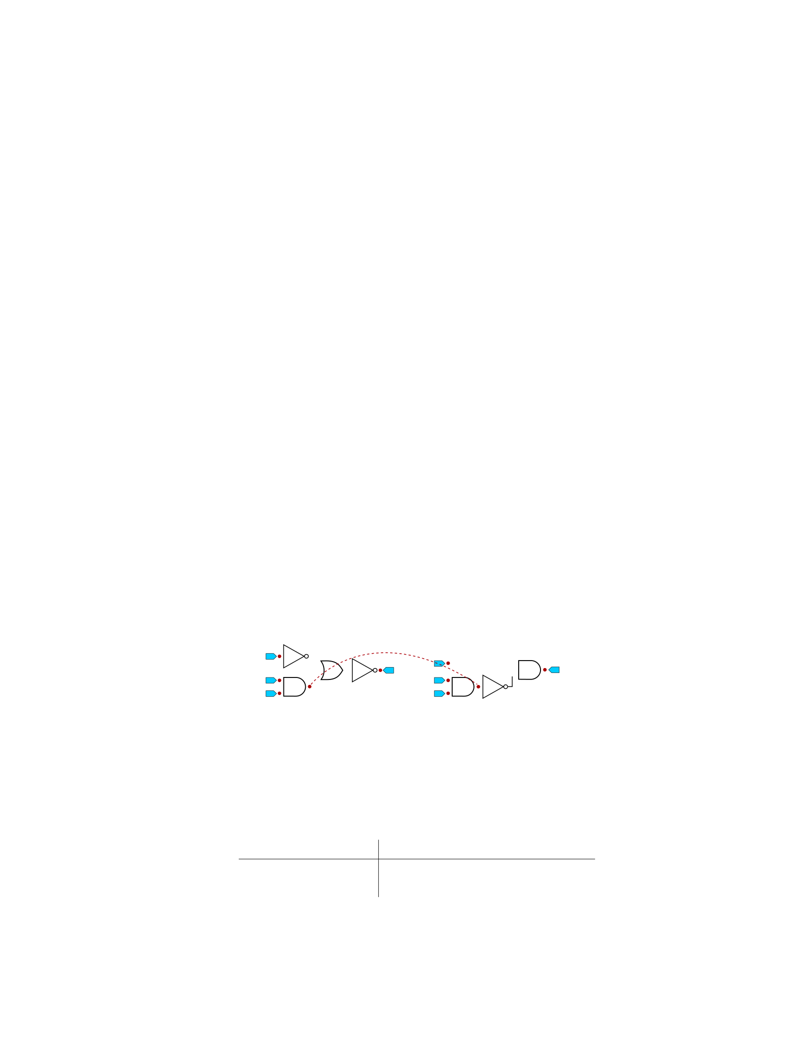
optimization is not possible (or needed) within the boundaries of that region. The definition
of Invariant Cone used here is not tied to module boundaries, and thus leverages intra-module
optimizations. Since LiveSynth does not artificially define partitions, the QoR impact is
substantially reduced.
Functionally-Invariant Boundaries (FIBs) [30] are the endpoints of invariant cones.
A FIB is a net in the design whose logic function has not been changed during synthesis,
regardless of how it is implemented. Global inputs and outputs are (always) FIBs, if retiming
is not applied flops are also FIBs. A change due to a “don’t care” condition is considered a
functional change and thus, the node is not a FIB.
In the example in Figure 4.2, the synthesis process may change the implementation
of the logic function f =!(!a + bc) to f = a·!(bc). In this case, there are two Invariant Cones:
fib1 = bc and fib2 =!a·!fib1. Note that internal nodes in fib2 presented logic changes and thus do
not constitute an Functionally-Invariant Boundary.
Table 4.1 shows statistics of the number of gates per Invariant Cone for some
Figure 4.2: Functionally-Invariant Boundaries provide a natural boundary for incremental
synthesis.
Table 4.1: Invariant Cones provide a natural boundary for incremental synthesis. Most of the
Invariant Cones present in the benchmarks tested are smaller than the proposed target.
Invariant Cone Size al dx fp mo or
< 200 3825 2489 1769 2702 643
200 − 300 10 35 99 161 172
93
A
B
C
Y
(a) Specification
A
B
C
Y
(b) Implementation
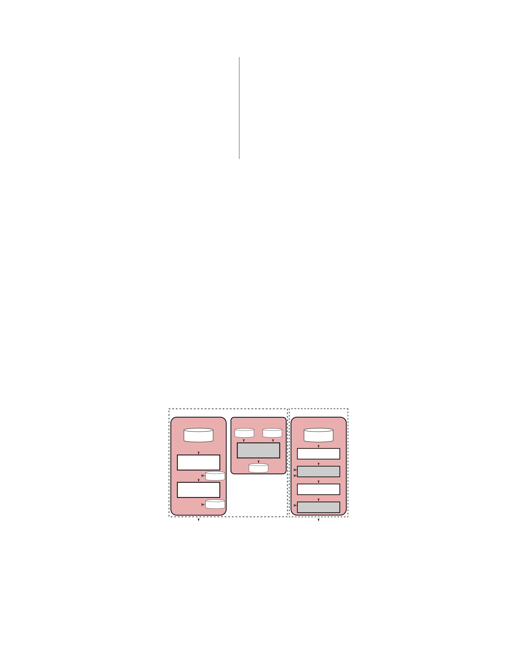
300 − 400
400 − 500
500 − 600
600 − 800
800 − 1000
> 1000
91
138
10
5
18
46
47
8
22
43
13
10
938
1
649
34
33
6
136
83
106
1
0
0
156
185
74
63
58
56
circuits (details in Section 4.5). The block sizes are smaller than the target established for
LiveSynth, which means that they can be easily combined for when a change affects multiple
Invariant Cones but also to attach neighboring regions in cases where the critical path is split
into multiple blocks.
4.3.4 LiveSynth flow
The overall flow of LiveSynth is depicted in Figure 4.3, and consists of two phases:
the Setup phase and the Live phase. The Live phase is split into three steps: Netlist diff,
∆Synthesis, and Netlist stitch. The Setup phase identifies FIBs (and respective Invariant
Cones) between the Spec0 and Impl0 after the initial synthesis. After setup in the Live phase,
when a change is made in the RTL, the changed file passes
94
HDL
Elaboration
Synthesis
Functional
Match
Initial Synthesis Setup Pass
∆HDL
∆Elaboration
∆Synthesis
Netlist Di ff
Netlist Stitch
spec0
impl0
spec0 impl0
FIBs
Place & Route Place & Route
Setup Phase Live Phase
Interactive
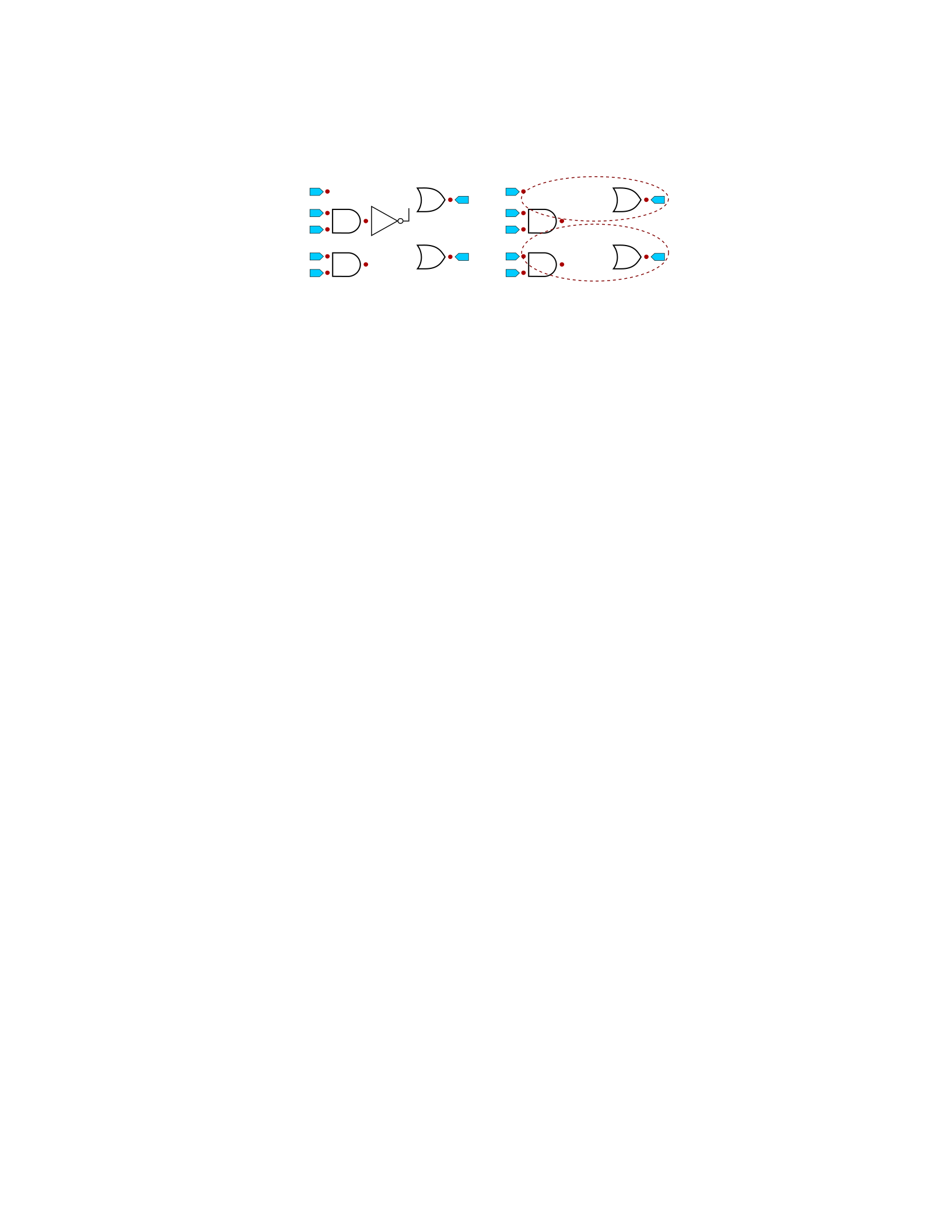
Figure 4.3: LiveSynth extracts a small subset of the design for synthesis and merges it back
into the original synthesized netlist, quickly achieving results comparable to the non-
incremental synthesis. Place and route are not included.
Figure 4.4: A single code change can impact multiple invariant cones that will need to be
synthesized.
elaboration, and the modified netlist is structurally compared to Spec0. The structural
comparison (Netlist diff) only matches the portions of the netlist that are identical in their
logic structure, and thus has linear complexity with the module size [30]. The main goal of
this pass is to identify which Invariant Cones have been changed.
The final incremental synthesis region can include multiple cones. This is because a
single code change may affect multiple cones, due to the overlapping nature of cones. This is
depicted in Figure 4.4, which shows a single gate change in a design that affects two
Invariant Cones (marked with the dashed ellipses).
After Netlist diff, the extracted netlist containing all the modified Invariant Cones is
synthesized. Then, the resulting netlist replaces the equivalent Invariant Cones in the original
synthesized netlist. Note that only the small region that was modified is synthesized during
the LiveSynth step, which is a key factor for synthesis speed.
4.3.4.1 Setup phase
95
a) Original( b) Modi( fied

The main goal here is to find FIBs and which gates belong to each cone, as well as
to how many cones a given gate belongs to. By knowing which gates belong to each cone,
LiveSynth avoids traversing the whole design when a change is made. Also, since cones may
overlap, a gate is only removed from the design when it belongs to zero
cones.
Since the structure of the logic changes during synthesis, it is not sufficient to
simply compare the netlists. Thus, LiveSynth relies on logic equivalence checkers (LEC) to
compare the elaborated and the synthesized netlists. To reduce the search space, I assume that
the synthesis flow has kept user-defined net names unchanged (except for appending instance
names), which I have observed to be true in all five flows tested (commercial and open
source).19 Then, LECs compare the function implemented by each of the logic cones. To
account for retiming (i.e., changing of flop position) that may have occurred during synthesis,
the method also counts the number of flops between each pair of FIBs. Although this is a
very long step, it only needs to be performed once in a while (prior to the execution of the
flow) and not for every code change, so this is not a huge problem. Also, if needed, this time
could be mitigated with better integration with the synthesis flow to keep track of FIBs [30].
4.3.4.2 Live phase
After setup, the LiveSynth flow enters a interactive phase that provides designers
feedback within a few seconds. This Live phase consists of cycling through three steps each
19 It is fine to miss some equivalency between nets, this only increases the size of regions, but does not
jeopardize the method as a whole.
96

time a designer makes a valid change, defined as any change that produces valid code. If a
change is not valid in syntax, the Live phase is not ran.
The Netlist diff step finds which portions of the netlist have changed. Netlist diff
compares the modules that have been changed (identified by system time stamp) of Spec1
with the original modules of Spec0. It traverses the netlist, starting at each FIB and going
backwards, until a new FIB is found. If a difference is found, that cone needs to be
synthesized. If the traversal does not spot a difference in the netlist, the synthesis results for
that region can be kept.
This structural comparison is fast since it only matches logic that is implemented in
the exact same way. Note that to make this search fast, I assume that nets with the same ID
are equivalent. Then, the search itself is responsible for proving that the two cones are
structurally, and thus, functionally identical. The ID is the concatenation of instance names
and the net name in the leaf instance. This allows for
uniqueness of identifiers.
The Netlist diff pass also keeps track of which gates are part of the cone, and thus at
the end of the pass, the gates that need to be synthesized are known. After the comparison, all
cones that were marked as different are treated as a single region for the next steps. The
process is depicted in Algorithm 1.
Algorithm 1 Netlist diff algorithm
1: procedure diff(FIB old, FIB new)
2: diff_cone ← Set.new
3: same ← same_operation(old.op,new.op)
4: for idx gets 0; idx < new.fanin.size; idx++ do
5: if ! is_fib(fanin(new,idx)) then
97

6: diff_cone.append(fanin(new,idx))
7: same ← same & diff(fanin(old,idx),fanin(new,idx))
8: end if
9: end for
10: return [same, diff_cone]
11: end procedure
After Netlist diff, the marked cones are extracted from the context of the design, and
synthesized on their own (Figure 4.5) in ∆Synthesis. Inputs and outputs to the region are
carefully set to prevent optimizations in the synthesis flow to simplify away logic that should
have been kept. Moreover, since the block being synthesized does not necessarily begin and
end in flops, I also set input and output delays according to the ones reported in the original
synthesis for those nets. This forces the synthesis to account for the delay of the logic that
was not included in the block. Timing constraints are also set in accordance with the original
design.
After the delta synthesis, the resulting netlist needs to be reattached to Impl0 to
create Impl1 in the Netlist stitch step. Also, any unused nets and gates need to be removed
since synthesis will not be triggered over the whole design. Thus, Netlist stitch first inspects
each gate in the original Invariant Cone and decrement the counter on how many cones the
gate belongs to, removing from the design any gate that reaches
98
Figure 4.5: Instead of triggering synthesis in the whole design, LiveSynth extracts the region
that needs to be synthesized. This is a key point for speed in LiveSynth.
the count of zero cones (Algorithm 2).
This procedure is sub-optimal for area, since it may result in redundancy. This
overhead is small for each synthesis increment, but may accumulate over the course of
multiple changes. However, note that a small increase in area (of around up to 5%, observed
by [43]) is generally more tolerable than the same increase in delay.
Algorithm 2 Netlist stitch algorithm
1: procedure stitch(Impl0, new_gates, old_gates, gate_count)
2: for all gate ← old_gates do
3: gate_count[gate.id]–
4: if gate_count[gate_id] == 0 then
5: remove(Impl0, gate.id)
6: end if
7: end for
8: for all gate ← new_gates do
9: insert(Impl0, gate.id)
10: end for
11: end procedure
4.3.4.3 Dealing with delay degradation
To reduce delay penalties, when a critical path crosses the boundary of the changed
region, the neighboring region is also included in for synthesis. This increases the runtime,
99
(a) Full Design
Delta Module
(b) Incremental Region

but reduces delay impact on the final circuit. Another possibility would be to extend the
partition definition, so the critical paths always lie within a region. One option not explored
here is to trigger a second incremental synthesis when there is frequency degradation,
however, it is not possible to know if the degradation is due to the flow or the change
introduced.
4.4 Structural Matching
In the previous section, I have described LiveSynth, an incremental synthesis flow
that aims to synthesize a circuit in a few seconds, after a small change. However, LiveSynth
stops after synthesis. It could be tied to existing incremental place and route tool, as those
existing in commercial FPGAs flows described in Chapter 3, however, as the results there
show, those do not meet the LiveSynth targets. In this section, I describe SMatch, a method
that allows a flow to leverage existing placement and routing results and reduce the amount
of work needed to generate a fully placed and routed netlist after a small code change.
4.4.1 Structural Matching of Netlists
SMatch is based on two key observations: 1) placement and routing are agnostic to
logic function and only depend on netlist structure and the physical dimensions of its
components, 2) in FPGAs, the elements of a netlist can only be a handful of types, and thus
there is a large number of equal objects in the netlist.
From the first observation, it is possible to conclude that structurally similar netlists
will be placed and routed in similar ways. At this point it is important to recognize that small
variations in a netlist can cause important variations in the optimal result of placement and
100
routing. However, the initial statement must be interpreted in the perspective of modern
incremental synthesis, which allows small perturbations (less than a few percent) on QoR.
Then, re-using an existing placement and routing will most likely yield similar QoR results.
Figure 4.6: After synthesis of modified cones, some LUTs are structurally equivalent between
the original and modified netlists. SMatch leverages that to reduce the amount of work
needed to do during placement and routing.
In general, this could be applied to any netlist for a target. However, for ASIC
netlists, the standard cell libraries are usually rich in types and sizes of cells. Moreover, in
ASIC flows, macros are often used to implement specific logic functions, such as arithmetic
functions, which introduce heterogeneity to the netlist and make it harder to find matches.
This makes the second key observation useful. In FPGA netlists, there are only a few types of
cells. Since LUTs with the same number of inputs are physically equivalent in an FPGA, it is
perfectly plausible to change the logic implemented by a LUT without the need to re-place
and re-route it, as long as the physical and logical connections with adjacent LUTs are
unchanged. Since not all LUTs will be matched, remaining LUTs need to be placed and
routed following conventional place and route
101

flow.
Therefore, the main challenge is to find the largest structurally matching region
after a change is introduced to the design in the minimum amount of time. This process is
illustrated in Figure 4.6, for the sake of simplicity and without loss of generality, it illustrates
LUTs with two input bits, however the method is trivially extended to any number of input
bits. Figure 4.6a shows an example of an initial netlist. Each LUT is named LUT_X with a
unique numeric ID, the function implemented by each LUT is indicated by a unique name.
Figure 4.6b, the change added only affected the final function implemented by a single LUT,
namely LUT_1, from f1 to g1. A regular physical implementation flow would run placement
and routing for all the LUTs in the design. A smarter flow could fix the position of all the
LUTs, except for LUT_1, and run placement and routing for LUT_1. SMatch proposes to not
run placement and routing for any LUTs, and simply update the function implemented by
LUT_1, by changing the contents written to the table. Then, in Figure 4.6c, the change made
introduced an extra LUT, LUT_4. Since this is a new LUT, it will clearly need to be placed
and routed. However, the inputs for LUT_3 also changed, since it originally came from an
input, but now comes from another LUT. Therefore, LUT_3 will also be placed and routed.
LUT_1, however, also had its functionality changed, but will not require place and route,
since its inputs and outputs did not change.
One could argue that since LUT_3 will be most likely placed in a different position,
this could affect the ideal placement for LUT_1, thus it should also be replaced. Although this
is a valid observation, the evaluation that this is not needed to reach “close-to-ideal” results
102

and that the impact on QoR of not considering those cases for placement and routing have
low QoR penalty, which is compatible with the goals of SMatch and LiveSynth.
Since this is a structural pass over both the netlists, it can also be performed in
linear time with the size of block considered. The method is explained in Algorithm 3. In the
first loop (lines 5 to 17), candidate equivalent LUTs are found between the original design
and the newly synthesized netlist. Since outputs are fixed and each net has a single driver,
there is only one possible candidate LUT for the output nets. Then, for an arbitrary LUT
throughout the netlist, SMatch only considers the LUTs from the same input, that is, if the
functionality is still the same, but the inputs are in a different order, the LUT will be marked
as not equivalent. Then, in the second loop (lines 18 to 24), the algorithm verifies that all the
LUTs that were still not marked as not equivalent, have the same set (and order of inputs),
otherwise the LUT is marked for placement and routing.
After SMatch, matching LUTs are updated, and any additional LUT is placed and
routed using the conventional place and route tools available in the flow. Any LUT that is no
longer used in the new implementation of the circuit should be removed and made available
before placement and routing of remaining LUTs, since it will open up space for new LUTs
to be placed, which can improve QoR.
Algorithm 3 SMatch algorithm
1:
2:
3:
4:
5:
procedure smatch(new_gates, old_gates)
candidatesmatchesno_equivfor all BFS from outputs(new_gates)←←← map()∅∅ do
6:
7: currentif is-output(current)← BFS.next then
103

8:
9:
elsecan ← same_output(old_gates)
10:
11:
end ifcan ← fan-in(candidates[fan-out(current)])
12: if candidates[current] != can then
13: no_equiv += current
14: else
15:
16:
end ifcandidates[current] ← can;
17: end for//End BFS
18:
19: for allif fan-in(candidate) = candidates[fan-in(lut)]lut,candidate ← candidates do then
20: matches += lut
21: else
22: no_equiv += lut
23: end if
24: end for
25: return no_equiv, matches
26: end procedure
4.4.2 Handling Retiming and extra registers
Retiming is the operation of moving logic across registers to improve timing
closure [60,71]. Retiming can be applied to any circuit without changing the sequential
behavior of it. Adding registers to a design is also an alternative for timing closure. They can
be manually inserted, inserted through the assist of automated tools [53], or even in latency
insensitive designs [39,86]. Regardless of the technique used, SMatch needs to handle those
changes in an efficient manner.
The main observation here is that, in FPGAs, adding, removing or moving flip-
flops is a simple operation due to the FPGA architecture and organization. FPGA
LUTs are organized in slices (Xilinx FPGAs) [108], or equivalently ALMs (Adaptive Logic
Module, in Intel FPGAs) [7]. The overall architecture of a block vary by vendor. In Xilinx
slices, there are 4 LUTs, with hardened arithmetic logic, 4 flip-flops, and bypass logic. The 4
LUTs can have different number of inputs in different slices (from 2 to 6). They can be used
104
independently, or combined into larger logic blocks (of up to 6 inputs). In any configuration,
there is at least one flip-flop per LUT. In Intel FPGAs, each ALM contain an 8-input
fracturable LUT, two full adders and four flip-flops. The fracturable LUT can be split into
pairs of LUTs of up to 6-input. Combinations that total less than 8 inputs can have
independent inputs, however, combinations that exceed the amount of available inputs need
to use shared inputs. For instance, to implement two 5-input LUTS, two inputs need to be
shared [5]. In the Intel FPGA case, the number of flip-flops is also enough to handle any
configuration, there is at least one
Figure 4.7: SMatch leverages the fact that each LUT has a flip-flop in its output that can be
activated/deactivated without impacting which routing resources will be used.
flip-flop per LUT and per adder. Also, in the case of both vendors, regardless of the flip-flop
usage in each LUT, the routing resources from the output of the slice are the same. Figure 4.7
depicts a simplified version of the architecture of both Xilinx and Intel FPGAs.
Thus, SMatch can simply add or remove flip-flops at the output of each LUT to
increase the amount of matching LUTs between two netlists. Simply put, during the SMatch
pass, registers can be ignored, and a final pass over flops only can add or remove flip-flops to
match the modified netlist.
105

One could imagine a FPGA architecture where less flip-flops exist, and thus the
simple approach of deciding where to use flip-flops after SMatch run is not viable anymore.
In those cases, it would be possible to adapt SMatch to: while doing SMatch, verify whether a
flip-flop is needed for each LUT and if so, verify if one exists, in this case, no extra work is
needed. In case a flip-flop is needed and one is not available, the
LUT is marked for placement and routing.
4.4.3 Partitioning the design size
Thus far, I have discussed how SMatch works, but not where it should be applied.
In theory, the method to find the matching LUTs could be applied to an entire modified
design, but that would be inefficient because it would require the synthesis of the whole
design, even for a small change. Moreover, synthesizing the whole design, even after a small
change, may yield important differences in the final netlist. Thus, SMatch is tied with
LiveSynth to reduce the region where it needs to be applied.
SMatch uses the same setup and Netlist diff methods as specified by LiveSynth.
However, instead of simply replacing the whole incremental synthesis block, as it would be
done in LiveSynth, SMatch is run. Then, instead of placing and routing the whole incremental
block, matching LUTs are updated, and only LUTs that do not match are placed and routed.
The final SMatch flow is depicted in Figure 4.8. The invariant regions are found
during a setup step, which is run once after the initial synthesis. It is reused across multiple
incremental steps and can be recalculated, ideally when no changes are being performed over
the code. When changes are being performed, the incremental step is used. It consists of three
main substeps: Netlist diff, synth, SMatch. Netlist diff compares the elaborated netlist from
106
the original code with the elaborated netlist of the modified code, keeping track of which
invariant cones were changed. Then, these invariant cones are synthesized, with aggressive
optimization goals. Finally, during
SMatch, the newly synthesized netlist is structurally compared against the equivalent
Figure 4.8: SMatch replaces placement and routing for a subset of cells changed in a design
during incremental synthesis. This allows to reduce place and route time.
region of the original synthesized netlist. Matching LUTs have their logic updated; while
unmatched LUTs are removed, replaced with newly synthesized LUTS, that are then placed
and routed. Both Netlist diff and SMatch are a simple pass over the graph, with simple
comparisons across cells in each and therefore are linear with respect to the
netlist size.
4.5 Evaluation Setup
LiveSynth and SMatch were implemented in C++14, compiled with CLANG
5.0.0, based on the open-source LGraph, a graph representation for VLSI design [92].
Synthesis is performed with YOSYS [105] version 0.7+312, a tool based on ABC [22],
107
HDL
Elaboration
Synthesis Functional
Match
Initial Synthesis
Setup Pass
∆HDL
∆Elaboration
FIBs
Setup Phase Incremental Phase
Interactive
Place &
Route
∆Place &
Route
Netlist Di ff
∆Synthesis
Structural
Match

targeting Xilinx FPGAs. Placement and Routing were done using Xilinx Vivado 2017.2, QoR
results are reported after routing. For LiveSynth only the complete incremental region is re-
placed and re-routed after a code change. I compared QoR after each change for each
incremental flow with full synthesis, independently for each change. For the structural
updates, the TCL interface of Vivado was used, I estimated the overhead of using the TCL
interface to guarantee that it was acceptable. For incremental updates in placement and
routing, the TCL interface was again making sure only the relevant cells were placed and
routed. The experiments were run on 2 Intel(R) Xeon(R) E5-2689 CPUs at 2.60GHz, with
64GB of DDR3 memory, ArchLinux 4.3.3-3 server.
First, the runtime for synthesis of LiveSynth LLIR [30] and an incremental
commercial synthesis flow for FPGAs are compared. LLIR is also implemented on top of the
same baseline as LiveSynth for fairness. The commercial flow is completely independent of
this flow. Then, the synthesis, placement and routing runtimes are compared for SMatch,
LiveSynth and an incremental placement and routing flow from a commercial FPGA vendor.
LiveSynth and SMatch share most of the same implementation infrastructure, however, the
final SMatch algorithm is applied to reduce the amount of placement and routing needed.
I used the Anubis benchmarks [89], described in Chapter 3. Briefly, Anubis
includes five designs (DLX, ALPHA, FPU, MOR1KX, OR1200) and code changes from real
changes done to the code during its development cycle. Design changes were taken from
repository commits. Each benchmark includes around 20-30 code changes, divided into three
categories: NoChange, Local, Global. NoChange are code changes that do not affect the logic
108

(renames, double inversions, so forth), Local affect a single module and Global affect either
multiple modules or modules that are instantiated multiple
times.
4.6 Evaluation
The evaluation begins by looking at the runtime of LiveSynth for synthesis only.
Since the same overall flow is shared for SMatch. LiveSynth is compared with LLIR and a
commercial FPGA flow for runtime. Then, I consider the runtime for synthesis, placement,
and routing for both LiveSynth and SMatch, comparing with the incremental placement and
routing flow from a commercial incremental FPGA flow.
To provide more insights on how SMatch can achieve speedups over LiveSynth, I
looked into the runtime of changing the functionality of a few hundred LUTs, changing their
placement, and changing their routing. SMatch is trading off placement and routing for the
structural comparison of the netlist.
Finally, I report the overall speedups for each flow, considering synthesis,
placement and routing and I looked into QoR results from each flow to show the quality
differences between a full synthesis and the incremental synthesis.
4.6.1 Incremental Synthesis Runtime
I first look into runtime for synthesis only. Figure 4.9 show the absolute runtime
numbers for the three incremental synthesis flows tested. LiveSynth had on average, across
benchmarks and across design changes, runtime of less than ≈ 7s to deliver a fully
synthesized netlist when applying a change to the RTL. Elaboration was the slowest task,
109
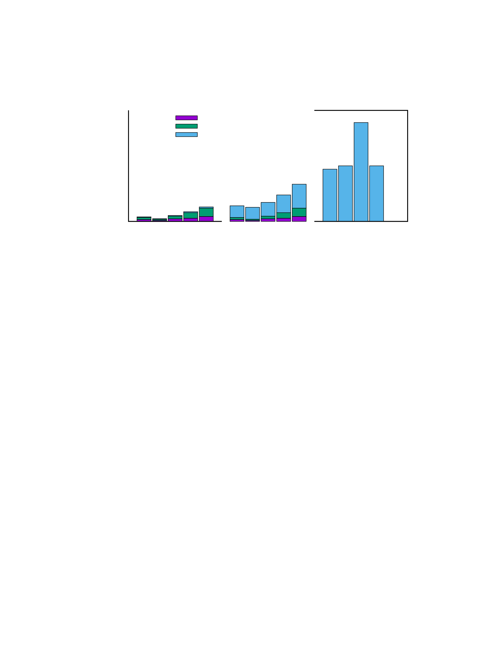
since it sometimes requires parsing and elaborating relatively large modules. LLIR was over
3× slower than LiveSynth on average. The main difference was the need to
Figure 4.9: LiveSynth improves the synthesis speed by an average of ≈ 10x compared to a
full synthesis. Each bar shows the runtime breakdown for various tasks up to synthesis. The
values reported are average across all the changes for each ANUBIS benchmark.
run synthesis on the full netlist, even though most of the netlist is already optimized at that
point, the synthesis tool still needs to, at least, traverse the whole design. The average for the
commercial flow was about 50s, and the flow did not finish for or1200 due to resource
constraints on the FPGA.
Both LiveSynth and LLIR have large variation in the speedup results, which is
expected since each change to the RTL has a different impact in the final design. In relative
terms, LiveSynth was typically 10× (or more) faster than the full baseline flow, while LLIR
was in general only 2× faster. Both flows presented large variability, with speedups from as
low as 10 − 20% to as high as 80× for LiveSynth and 32× for LLIR.
110
0
20
40
60
80
100
dlx
alpha
fpu
mor1kx
or1200
Synthesis Runtime (s)
LiveSynth
Elab
Di ff
nthSy
dlx
alpha
fpu
mor1kx
or1200
LLIR
dlx
alpha
fpu
mor1kx
or1200
Commercial
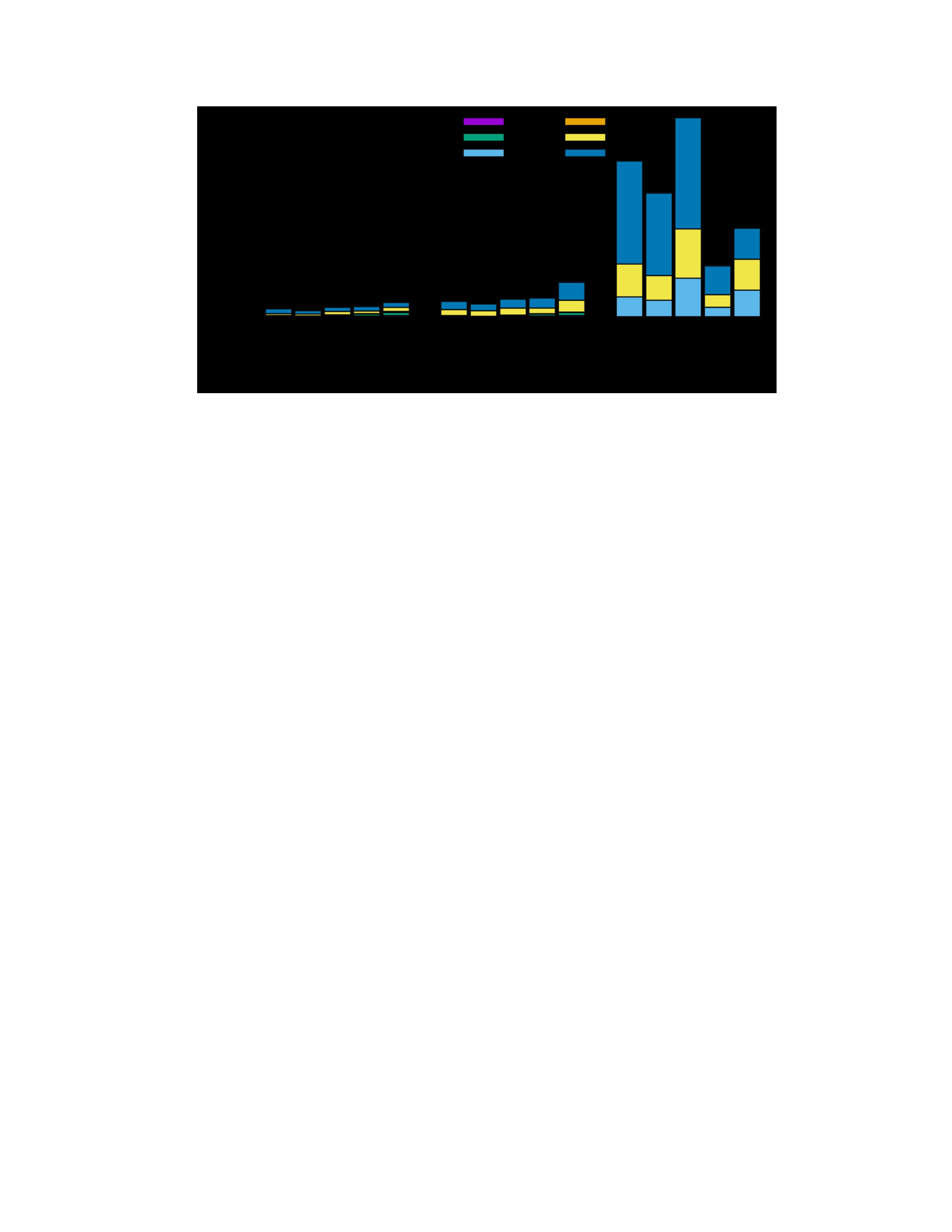
Figure 4.10: SMatch performs synthesis placement and routing in under 30s for most changes
in the Anubis benchmark suite. This is faster than the incremental flow of the commercial
flow and LiveSynth, the state-of-the-art academic incremental flow.
4.6.2 Complete Flow
Overall, SMatch has a runtime of under 30 seconds for synthesis, placement and
routing, for most changes in the Anubis benchmark suite, with an average of around 21s. This
is around 1.6 to 2× faster than LiveSynth on average, and 5 to 21× faster than the incremental
mode of the commercial flow. Figure 4.10 reports the runtime for each flow, for each
benchmark in the Anubis suite, averaged across all changes and broke down by step in the
flow.
Most of the SMatch synthesis routine is the same as LiveSynth, however, SMatch
has a more elaborated merge step (the Structural Matching algorithm). This adds to the
synthesis time, however, SMatch has the advantage of reducing placement and routing even
further. Since placement and routing are both slower that the simple
111

SMatch algorithm, SMatch ends up being faster than LiveSynth. SMatch is able to finish more
than 70% of the changes in less than 30s, while LiveSynth can only finish 31% in that time,
mostly changes that affect a very small number of gates.
In the commercial flow, there is no incremental synthesis step, the incremental flow
uses a full synthesis and then runs incremental placement and routing, trying to leverage
existing results for those steps. This explains the large portion of synthesis for the
commercial flow runtime results.
Figure 4.11 shows the same data as before, but with a more close view of the
runtime breakdown for LiveSynth and SMatch, normalized to 100%. Most of the time is spent
in placement and routing. Even though the proposed flows minimize the amount of routing
needed, they still rely on Vivado’s placer and router, which even in incremental mode is
meant to maximize QoR at all costs. This is true for both flows, but is more noted in
LiveSynth, since there are more wires to route in that case. SMatch trades off an added step
(SMatch) by reduced placement and routing times. The stitch phase of LiveSynth is not
visible on the plot since it only takes a few milliseconds. The main difference between
commercial flow and the other two is that since the commercial flow performs full synthesis,
there is usually a larger number of gates that is affected even after small changes.
The LiveSynth speedup comes from two different places. First, LiveSynth reduces
the amount of work during synthesis. Then, untouched gates are kept in its original
placement, and only changed blocks are re-placed and re-routed. Thus, there is also a
reduction in the amount of gates that need to be placed and routed.
Note that in SMatch the time spent in place and route is proportionally smaller
112
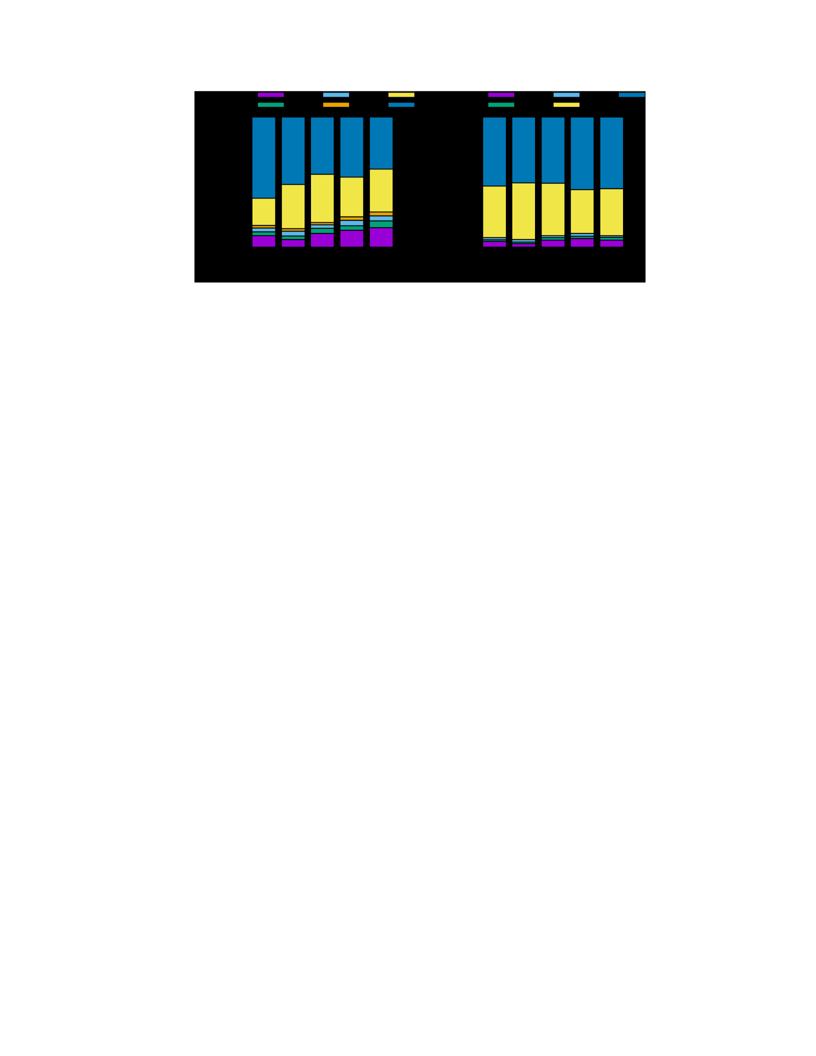
Figure 4.11: Most of the time is spent in placement and routing, that are both performed
without modification in Vivado.
than in LiveSynth. Placement account for only about 20% of the runtime and routing for an
average of under 50% of runtime in the SMatch flow. Another way of looking at it, is to
check how much time it takes to update a LUT as opposed to place and or route LUTs. I
performed a simple experiment where a design was fully synthesized, placed and routed, and
then performed three operations independently, in a varying number of LUTs: change LUT
functionality, place re-place LUTs, re-route LUTs. This was performed for ≈ 100,400,1000
and 5000 LUTs, since those are in the typical range for incremental synthesis. Results are
summarized in Figure 4.12.
Finally, this can be summarized by looking into the overall speedups for each
incremental flow against the respective full flow. Thus, the incremental commercial flow was
compared with a full synthesis, placement, and routing in the same commercial flow. SMatch
and LiveSynth were compared with full synthesis in Yosys, plus placement and routing in
Vivado. The overall speedup when running SMatch is over 20 times faster than a full
synthesis, placement, and routing run. It is also at least 1.6× and up to 300×
113
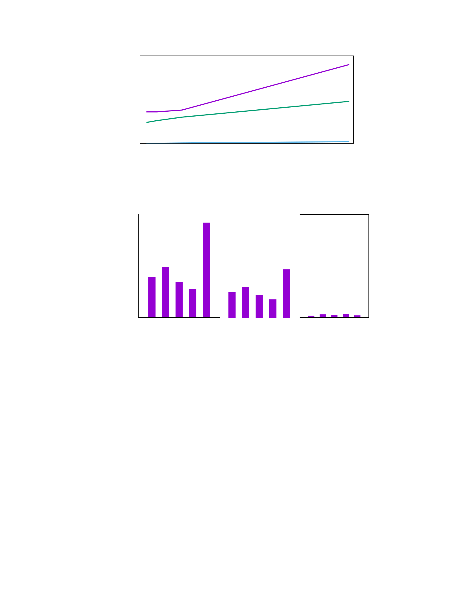
Figure 4.12: Place and route LUTs is orders of magnitude more expensive than simply update
the functionality of an already placed and routed LUT. The speedups of SMatch come from
that observation.
Figure 4.13: SMatch is able to deliver over 20× speedup over the full synthesis flow, since it
allows to reduce the amount of placement and routing needed in the full flow.
faster than full synthesis (maximum achieved when place and route are reduced to zero
during the incremental phases). SMatch is also 1.5 − 2× faster than LiveSynth, when
performing placement and routing only over the gates within invariant cones touched by the
code change. Those results are summarized in Figure 4.13.
When comparing the incremental mode of the commercial flow, it is only 30-
114
0
10
20
30
40
50
0 1000 2000 3000 4000 5000
Runtime (s)
Number of LUTs
Place Time
Route Time
LUT Update
0
10
20
30
40
50
60
70
80
SMatch LiveSynth Commercial
Speedup
dlx
alpha
fpu
mor1kx
or1200
dlx
alpha
fpu
mor1kx
or1200
dlx
alpha
fpu
mor1kx
or1200

80% faster on average than the full mode, being slower in some cases. There is a difference
in goal between the two flows presented here and the commercial flow. The commercial flow
is trying to optimize for QoR, while reducing the runtime. LiveSynth and SMatch are
carefully designed to maintain the QoR level of the full flows, but the main objective is to
reduce runtime. Therefore, even the incremental placement and routing mode in the
commercial flow are sometimes as slow as the full mode.
4.6.3 QoR degradation
I also looked into QoR degradation due to SMatch. Given the approach taken, I
expected that some degradation would be observed. I compare SMatch and LiveSynth against
the full baseline flow (synthesis, placement, and routing). In some cases there was increase in
frequency, but I report those cases as 0% degradation, since those are not due to the
incremental techniques, however I saw increases of up to 3% in frequency. The maximum
observed decrease in frequency was of ≈ 5% and more than 80% of the changes had < 0.5%.
A histogram of frequency degradation of all the changes in Anubis is shown in
Figure 4.14. In this experiment, I compared the degradation of running the incremental flows
versus a full synthesis in Yosys, plus placement and routing in Vivado. The figure shows what
percentage of changes, combining all benchmarks, observed a given amount of delay
degradation. For instance, over 70% had no delay degradation and only about 5% of the
changes had a degradation of about 1% in delay. The high number of changes with no
degradation is in part due to some changes not affecting the critical path, and
115

(a) LiveSynth (b) SMatch
Figure 4.14: In more than 80% of the test cases SMatch and LiveSynth delivered frequency
within 0.5% of a full synthesis flow. The maximum decrease in frequency was of ≈ 5%.
thus no change is observed. A comparison between the basic Vivado flow and the flows
synthesized in Yosys with Vivado place and route is out of the scope of this dissertation and
not included.
This small degradation in quality is compatible with the goals of this work of
providing fast feedback for small changes even with small degradation in QoR. For
deployment, this gap can be closed with a final step of full synthesis, but during
development, this small degradation is within acceptable ranges [89].
4.6.4 Setup overhead
Both LiveSynth and SMatch require a setup step, that needs to be run once before
the incremental steps can run. Even though a single setup run can be used across multiple
incremental updates, this is still undesirable overhead. The setup includes includes a full
synthesis, placement and routing, and finding invariant boundaries. Synthesis, placement and
routing time are not exactly overhead, since they would be ran before the change.
116
0
10
20
30
40
50
60
70
80
-5 -4 -3 -2 -1 0
% changes per degradation
Frequency Degradation (%)
0
10
20
30
40
50
60
70
80
-5 -4 -3 -2 -1 0
% changes per degradation
Frequency Degradation (%)

The routine to find the boundaries is the only added task. It requires a netlist after
elaboration and a netlist after synthesis. In my experiments, I noticed that finding the
boundaries takes about twice as much as the synthesis alone. For the benchmarks tested, that
ranged from 120 to 480 seconds. However, this overhead can be amortized over multiple
incremental changes.
4.7 Conclusions
Slow turnaround time for synthesis, placement, and routing are one of the main
bottlenecks in hardware design productivity. I believe that an interactive synthesis flow is
possible and would reduce design time by allowing faster iterations between code changes
and results.
In this chapter, I have presented LiveSynth– an incremental synthesis flow
independent of specific tools – and SMatch– an incremental flow optimized for FPGAs.
LiveSynth leverages natural invariant boundaries to reduce the impact of splitting the design
into regions while minimizing the impact on QoR. LiveSynth minimizes the amount of work
that needs to be done by: 1) only elaborating RTL files that were changed by the designs, and
2) avoiding launching synthesis over the whole design. When a critical path lies within the
boundaries of the incremental region, LiveSynth includes neighboring regions to reduce the
hit on frequency.
SMatch builds upon the idea of live turnaround, but attacks long placement and
routing times, while still looking at logic synthesis techniques. In particular, SMatch relies on
117

structurally matching LUTs and only changes the logic implemented by matching them,
leveraging existing placement and routing from previous runs.
The results show that LiveSynth is able to reduce synthesis time by an average of
10×. SMatch is up to 20× faster than existing incremental commercial FPGA flows. I also
showed that LiveSynth and SMatch have small impact on delay (frequency) for only a few
design changes but always smaller than 5%.
Future work will include looking for ways to further partitioning the synthesis
blocks, by leveraging logically independent blocks, but also at ways to handle unmatched
LUTs without the need to fully re-place and re-route them, always with low impact in
QoR.
Chapter 5
Conclusion and Future Opportunities
Imparare non stanca mai la mente.
Leonardo da Vinci
In this thesis, I have examined some of the problems in current hardware design
methodologies and describe some of my efforts to address these problems. The design of
domain specific hardware has emerged as a solution to the slowdown in the improvement of
single-thread performance observed in the last few years. As a consequence, hardware design
has attracted many domain specialists, who do not have a background in hardware
118

development and the contrast between modern hardware and software development cycles
became evident.
Recently, there have been multiple attempts to address the gap between hardware
and software development by improving the productivity of hardware designers, either by
increasing the abstraction of HDLs or trying to increase design reuse. The work that I have
presented in this thesis bears a different, orthogonal, direction, trying to improve the circuit
abstractions used by hardware designs and by improving the runtime of hardware tools.
Fluid Pipelines, a new hardware design style, allow tools to more efficiently change
the pipeline configuration of a design, by adding, removing or changing the position of
pipeline stages and thus improve the ability of designers to meet the timing constraints of the
design. Fluid Pipelines transformations can be applied at any stage of the design cycle
without the need to spend weeks of engineering time re-working the design to the new
specifications. Therefore, Fluid Pipelines reduces the early pressure on carefully specifying a
design before it is well known and understood.
Even though Fluid Pipelines can be applied late in the design cycle, to fully assess
the impact of those changes it is still necessary to get a post-routing implementation of the
circuit, which is often costly. Incremental synthesis techniques can leverage existing
synthesis results to create a synthesized design after small changes. In this thesis, I presented
the first benchmark for incremental synthesis, ANUBIS, that contains both RTL code and
design changes. ANUBIS is publicly available at https://github.com/masc-
ucsc/anubis. Thus far, research with incremental synthesis had been using arbitrarily
defined changes over designs and since those were not made publicly available, it was not
119

possible to fairly compare two various incremental flows. ANUBIS includes real changes,
taken from the design during design development to improve the representativeness of the
changes.
Finally, I presented LiveSynth and SMatch, two incremental synthesis flows that aim to
provide feedback for small changes in a few seconds. LiveSynth focuses on synthesis, the first
step of the implementation flow, whereas SMatch also tries to minimize the amount of work
that is needed to fully place and route a design. Both techniques operate over invariant cones,
i.e., cones whose functionality did not change during synthesis. After a change affected cones
are synthesized independently of the design, considerably reducing the runtime. SMatch also
tried to structurally match the netlist, without regards to logic of each cell, and then simply
replace the logic, avoiding the need to place and route matching cells.
The work presented here also opens up opportunities for new research. Any of the
ideas presented here can be used independently, however, there is a lot of synergy between
them. A single combined framework that can perform pipeline transformations and quickly
evaluate if those transformations yield better results would help advance the Pareto frontier
by improving both performance and energy. For changes that affect throughput, the missing
piece here is a “live” cycle accurate simulator. Although not part of this thesis, I am
collaborating in the development of such simulator.
Another important opportunity to further improve the work presented here is to
continue to develop new incremental steps, like an incremental placer and an incremental
router tools. SMatch can be easily applied to FPGAs, but its applicability to ASICs is limited
by size and aspect ratio of cells and macros. Thus, an incremental place and route tool could
120

improve the accuracy of LiveSynth when applied to ASIC designs. Finally, LiveSynth still
requires integration with incremental timing and power analysis tools to truly provide
feedback within a few seconds. Incremental timing tools have been studied and exist,
however, there has not been a lot of research on faster methods for power estimation.
I finish this PhD and this thesis positive that there is a lot of exciting opportunities
and challenging problems that need to be addressed. While I believe that this thesis is a good
step towards more efficient tools for hardware design, we, as a community, still have a lot of
work to do to establish hardware design techniques that are capable of the same level of
productivity that.
121

