


1
CHAPTER I
INTRODUCTION
Scientists across multiple fields, not just physics and astronomy, have an interest in comets
and their connection to the formation of the solar system. Many questions concerning the
chemical and biological evolution of life on Earth involve the early conditions of the planet.
Accretion of material in the outer distances of the solar system led to the formation of comets.
Initially postulated as “dirty snowballs” [40], recent observations of the composition of comets
led astronomers to view them more as “icy dirtballs”, consisting mainly of ice, rock, and organic
compounds that coalesced
togetherintolowdensitystructuresduringtheearlyageofthesolarsystem, over4.5billionyearsago
[3]. Thiscompositionappearstoholdtrueevenforobservedinsterstellarcomets, suchas2I/Borisov
[8], which was observed passing through our solar system in 2019. Comets are usually grouped
by their orbital characteristics, with the longer-period comets originating from distant small-body
populations such as the Kuiper Belt, the scattered disk, and the Oort Cloud. The existence of these
populations support a model of the evolution of the solar system known as the Nice model,
where the gas giants were in more cicular, closely spaced orbits at the edge of the inner disk.
Small icy bodies were scattered by the gas giants inwards, which caused Saturn, Uranus, and
Neptune to migrate outwards due to conservation of angular momentum [38]. Further
interactions with Jupiter caused the icy bodies to enter highly elliptical orbits, while Jupiter
migrated slighty inwards towards its current postion. An alternative model known as the grand

2
tack hypothesis proposes that Jupiter instead initially migrated inwards from a distance of 30 AU
and then outwards after capturing Saturn in a mean-motion resonance [26]. This hypothesis has
developed more recent support from studies of comets C/2014 S3 (PANSTARRS) and
67P/Churyamov-Gerasimenko, where the low detection of collisional elements in these outer
bodies corresponds with the early migration of Jupiter and Saturn posited in the grand tack [37].
Comets tend to be less dynamically active and exhibit less change in volatile composition
compared to other major bodies in the solar system. Thus, they provide insight into the physical
and chemical properties of the early conditions of the solar system. Insitu measurements of
comets, such as the Stardust mission, have detected organic molecules, including the amino acid
glycine [9]. Such evidence supports the hypothesis that comets were key to delivering the
precursors to life to early Earth. However, recent studies into comets, including the Rosetta
mission, have measured the Deuterium-to-Hydrogen (D/H) ratio, which was determined to be at
least three times greater than the ratio for the Vienna Standard Mean Ocean Water (VSMOW) on
Earth, (1.5576±0.0001)×10−4 [27]. This suggests the opposite to the long-held idea that comets
were also the means through which water came to our planet. Cometary science is still rapidly
changing and can still provide much in the way of constraints of the formation of Earth and the
solar system.
The majority of comets fall within two categories: short-period and long-period comets, based
on whether their orbital revolution periods are less than, or greater than, 200 years. Most short
period comets, known as Jupiter-family comets (JFCs), are theorized to have originated from
beyond Neptune, in the scattered disk of the Kuiper Belt region. They tend to orbit in the same

3
ecliptic plane as the planets and have periods of less than 200 years. The exception to these are
the Halley-family comets. While they also have a short orbital period, they are highly inclined to
the ecliptic, suggesting a different region of origin: the distant Oort Cloud. Proposed by Jan Oort
in 1950, the Oort Cloud is a theoretical, spherical region of space dominated by icy planetesimals
that were theorized to have formed during the same time period as the planets [32] [10]. Long-
period comets by contrast are highly eccentric, leading to orbital periods that range from
hundreds to thousands of years. These long-period comets are also thought to have originated
from the Oort Cloud. As many have hyperbolic trajectories, long-period comets will only have a
single solar apparition before they escape the solar system.
Due to their possible connection to the formation of the solar system, comets are the subject
of numerous chemical surveys [15]. Narrow-band photometry [1] and spectroscopic surveys [7]
have shown that the majority of comets are similar in chemical composition, with the exception
that a significant fraction of JFCs are depleted in carbon-chain molecules. Observations of the
dust-to-gas ratio and the abundances of carbon-based radical species (
𝐶𝑁
,
𝐶
3,
𝐶
2, etc.) show little
correlation based on composition or dynamical family. The subtle variances exhibited in the
comets based on their classes suggest differences in dynamical evolution rather than different
conditions of formation [7].
Due to the nature of comets, many properties have to be inferred from the types of radiation
we can detect remotely, as in situ observations are a rare opportunity. One such property is the
rotational period of the comet, which has most commonly been determined from the measured
lightcurve. If a celestial target such as a comet is observed over a long enough period, it is possible

4
to graph the flux or intensity of the measured light over time. If periodicity is seen in the
lightcurve, then it is possible to determine a spin period of the nucleus. Further constraints could
be made if multiple lightcurves are made over a range of heliocentric distances, as was made
with 1P/Halley [14]. Active areas are determined from spherical nucleus approximations, even
though they tend to be elliptical in nature. Constraints are made based on the size and flux of
emission sources, and are determined as fractions of the surface area of the nucleus [20].
1.1 Target comets
The comets examined in this research were C/2009 P1 (Garradd), Comet 168P/Hergenrother,
and Comet 10P/Tempel 2. Garradd was an active, dynamically young, long-period comet at the
time of observation, likely making its first trip through the solar system. The comet is in a highly
eccentric orbit of e = 1.001, and has an inclination of 106.18 degrees. Comet Hergenrother is a
Jupiter-family comet with an orbital period of about 6.90 years. It has an orbital eccentricity e =
0.610, and an inclination of 21.93 degrees. Tempel 2 is also a JFC, with e = 0.5363, an inclination
of 12.02 degrees, and an orbital period of about 5.5 years.
Comet Garradd was very active during its pre-perihelion transit, with one of the highest dust-
to-gas ratios and water production rates observed in a comet [5]. The
𝐶𝑂
2/
𝐻
2
𝑂
and
𝐶𝑂
/
𝐻
2
𝑂
ratios were measured from September-October 2011, and in January-March 2012, and were
found to be less abundant post-perihelion [5]. Since the ices in comets are primarily composed
of these volatiles, we can determine how the activity is driven during the comet’s passage. An
asymmetry between the two ratios from pre- to post-perihelion also suggests either a large-scale
chemical heterogeneity in the nucleus [30], or that the rotational state led to an effect where one

5
hemisphere was exposed to more activity from solar exposure than the other [13]. It also had a
high active surface area to nucleus area ratio.
Comet Hergenrother was a recently discovered comet, of which few publications exist. It
underwent an outburst in 2012, which may have resulted in a fragmentation event a few weeks
afterward and has been reported as overdue for its 2019 apparition after it was not detected
near its expected perihelion passage. [41]. Pierce and Cochran [33] performed spectroscopic
analysis of Hergenrother and found it to be the most depleted comet reported in
𝐶
2,
𝐶
3, and
𝑁𝐻
2.
Observations of such events can provide unique insight into the chemical and physical properties
of comets during a period of high activity. Fragments of Comet 73P/Schwassmann-Wachmann 3
were observed to have similar chemical properties but physical heterogeneities [16]. The
fragmentation event itself can also affect the dust production, such as with C/1994 S4 LINEAR [2],
or the orbital parameters, as with the Kreutz sungrazers, a family of comets believed to have
originated from a common progenitor comet that fragmented into two parts during a past
perihelion approach within 3.45 solar radii [19]. These super-fragments were then believed to
have undergone their own fragmentation events upon subsequent perihelion passages [36].
In contrast, 10P/Tempel 2 has been extensively studied since its discovery in 1873. Its short
orbital period, allowing for multiple observations over dozens of apparitions, as well as it once
being a possible target for a flyby mission, has made it the object of numerous ground-based
studies. Its next close approach to Earth is due to occur in August 2026 with a nominal geocentric
distance of 0.41 AU. It has been observed to have low outgassing activity and brightness pre-

6
perihelion, and has a typical dust-to-gas ratio of other comets with a similar perihelion distance
[23].
CHAPTER II
OBSERVATIONS
Observations of comets primarily focus on two components: the nucleus and the coma. The
nucleus corresponds to the solid part of the comet. Nuclei are typically comprised of dust and
ice, and tend to have a size range on the order of a few to tens of kilometers. As the nucleus is
exposed to heat from the Sun, the ices trapped on or below the surface can sublimate. The
resultant atmosphere of gas surrounding the nucleus is known as the coma. As the comet
approaches the Sun, the visible coma can increase in size to an order of tens of thousands of
kilometers in diameter, as ice grains can continue to sublimate as they’re dragged outwards by
the gas. Due to the low albedo and smaller size of the nucleus compared to the coma, direct
observations of the nucleus are usually restricted to in situ measurements. For comets Garradd
and Hergenrother, the measurements for this study were taken of their respective comae from
ground-based telescopic observations. The observations for Comet Garradd were obtained pre-
perihelion, while the Hergenrother and Tempel 2 observations were obtained post-perihelion.
Specific observation and calibration parameters for Garradd, Hergenrother, and Tempel 2 are
shown in Table 2.1 and Table 2.2 on page 8.
ThecomaobservationswereobtainedwiththeGeorgeandCynthiaMitchellSpectrograph. This
integral-field unit (IFU) spectrograph is a low- to moderate- resolution fiber optic spectrograph

7
consisting of 246 optical fibers. The optical fibers each have a diameter of 4.1 arcsec and are
arranged in a 1.7 x 1.7 arcmin array, alternating from 14 to 15 bundled fibers per row [17]. A
diffraction grating covered the passband from 3600-5800 Å and provides a spectral resolving
power (
𝜆
/Δ
𝜆
) of 850. The spectrometer was used in conjunction with the 2.7 m Harlan J. Smith
Telescope located at McDonald Observatory in Fort Davis, Texas. In order to maintain the comet’s
position on the array, a tracking star is used with a fiducial that moves opposite to the comet’s
motion. Any star spectra caught crossing through the field of view are removed in analysis [33].
Observations were taken of various radical species with spectral emission bands visible in
the spectrometer’s passband, including
𝐶
2,
𝐶
3,
𝐶𝐻
,
𝐶𝑁
, and
𝑁𝐻
2. Each fiber in the array was
connected to a charge-coupled device (CCD) and yield independent spectra. The raw data were
initially reduced through bias subtraction, flat fielding, and calibration in flux and wavelength.
Since the measured spectra are a mix of the emission bands from the coma superposed on a
continuum from the reflection of the solar spectrum off the dust in the coma, analogue stars
were utulized. Each night the flux and color of a solar analog star is matched with the observed
comet’s spectrum, and the solar spectrum is subsequently removed.
Table 2.1
Comet Observation Parameters
Comet
Obs. Date
r
𝐻
1
Δ2
Phase Angle3
Pre/Post
(UT)
(AU)
(AU)
(Degrees)
Perihelion
10P/Tempel 2
2010 Jul 15
1.43
0.72
42.2°
Post
2010 Sep 13
1.60
0.67
21.8°
Post
C/2009 P1 (Garradd)
2011 Aug 20
2.28
1.40
16.1°
Pre
2011 Aug 21
2.27
1.39
16.4°
Pre

8
2011 Aug 22
2.26
1.39
16.9°
Pre
168P/Hergenrother
2012 Oct 6
1.42
0.44
14.8°
Post
2012 Oct 8
1.42
0.44
16.1°
Post
2012 Oct 9
1.42
0.44
16.7°
Post
2012 Dec 19
1.66
0.99
32.7°
Post
2012 Dec 20
1.66
0.99
32.7°
Post
2012 Dec 21
1.67
1.00
32.7°
Post
Table 2.2
Comet Calibration Targets
Comet
Obs. Date (UT)
Flux Standard
Solar Analogue
10P/Tempel 2
2010 Jul 15
Feige 98
None
2010 Sep 13
BD+25 3941
HD 191854
C/2009 P1 (Garradd)
2011 Aug 20
BD+25 3941
39 Tau
2011 Aug 21
Feige 15
HD 6204
2011 Aug 22
BD+28 4211
HIP 109931
168P/Hergenrother
2012 Oct 6
Feige 15
HD 19518
2012 Oct 8
BD+28 4211
HIP 109931
2012 Oct 9
BD+28 4211
16 Cyg B
2012 Dec 19
Feige 15
Hyades 64
2012 Dec 20
Feige 34, Feige 56
35 Leo
2012 Dec 21
Feige 15, Feige 25
Hyades 64, HD19518
The reduced data were separated into columns representing the fiber number, the base-10
logarithm of the projected distance from the comet nucleus (
𝑙𝑜𝑔
(
𝜌
)), the logarithm of the column
density of the respective radical (
𝑙𝑜𝑔
(
𝑁
)), and the
𝑥
and
𝑦
coordinates of the coma measurement
from the comet nucleus. For the Garradd and Hergenrother data,
𝑥
corresponded to the hour

9
angle offset in kilometers, and
𝑦
corresponded to the declination position in kilometers. The
radial distance from the comet nucleus,
𝜌
, was determined by the distance formula
√︃
𝜌
=
𝑥
2 +
𝑦
2 (2.1)
The optocenter fiber was determined from each observation from the fiber corresponding to the
lowest value of
𝜌
. This single fiber is designated as the position of the comet nucleus.
Raw contour plots were generated for each observation, with the variables corresponding to
the
𝑥
and
𝑦
values for each observation, and the contour levels corresponding to the
𝑙𝑜𝑔
(
𝑁
) values.
The data were then analyzed based on their arrangement about the optocenter. In order to model
enhanced coma features as a function of projected distance from the nucleus, azimuthal rings
were determined based on the fibers being arranged in concentric, hexagonal rings about the
optocenter.
For each pixel in the ring, the projected distance was measured from the optocenter by
√︃
|
𝜌
−
𝜌
0| = (
𝑥
−
𝑥
0)2 + (
𝑦
−
𝑦
0)2 (2.2)
where
𝑥
0 and
𝑦
0 representthehorizontalandverticalpositionoftheoptocenter,and
𝑥
and
𝑦
represent
the horizontal and vertical position of the respective pixel. For each pixel in each azimuthal ring,
the values for |
𝜌
−
𝜌
0| were averaged, yielding an averaged radius value (
𝜌𝑎𝑣𝑔
). The column
densities for each fiber in the ring were also averaged, yielding an azimuthally averaged column
density value
𝑁𝑎𝑣𝑔
. In order to describe the relationship of the column density of each radical
with respect to the projected distance from the nucleus, a relationship
𝑁𝑚𝑜𝑑𝑒𝑙
was determined,

10
𝑁𝑚𝑜𝑑𝑒𝑙
=
𝐶
|
𝜌
−
𝜌
0|
𝑘
, (2.3)
where
𝐶
and
𝑘
are constants determined from a weighted least-squares fit. The fit parameters
were determined from the linear relation
log(
𝑁𝑚𝑜𝑑𝑒𝑙
) =
𝑘
log(|
𝜌
−
𝜌
0|) + log(
𝐶
) (2.4)
To further examine the heterogeneities of the radicals, azimuthal division coma enhancement
plots were generated, with the contour levels corresponding to the column density
𝑁
of each
fiber divided by the respective
𝑁𝑎𝑣𝑔
of the azimuthal ring. Radial division coma enhancement
plots were generated in a similar manner, with the contour levels corresponding to the ratio of
𝑁
over
𝑁𝑚𝑜𝑑𝑒𝑙
for each fiber in the array.
These azimuthal and radial coma enhancements can be used to look for coma features such
as jets or arcs. In addition to comparing coma features for each radical species across different
comets, they can also be used to observe how these features change over time. By focusing on
how the features change in position over several observations, we can attempt to link coma
features with changes in the physical nucleus, and recurring coma morphological features can be
used to constrain possible rotational states of the comets. The most common way to constrain
comet rotation periods is through analyzing a measured lightcurve to look for periodic, repeating
behavior [31]. A technique similar to ours used by Esterle [11] with Comet Halley involves
dynamically modeling simulated dust jets about the long axis mode of the comet nucleus over
time, and comparing them with jets seen in ground-based observations. Comparing

11
spectroscopic features allows for an additional method of analyzing rotation by use of a Monte
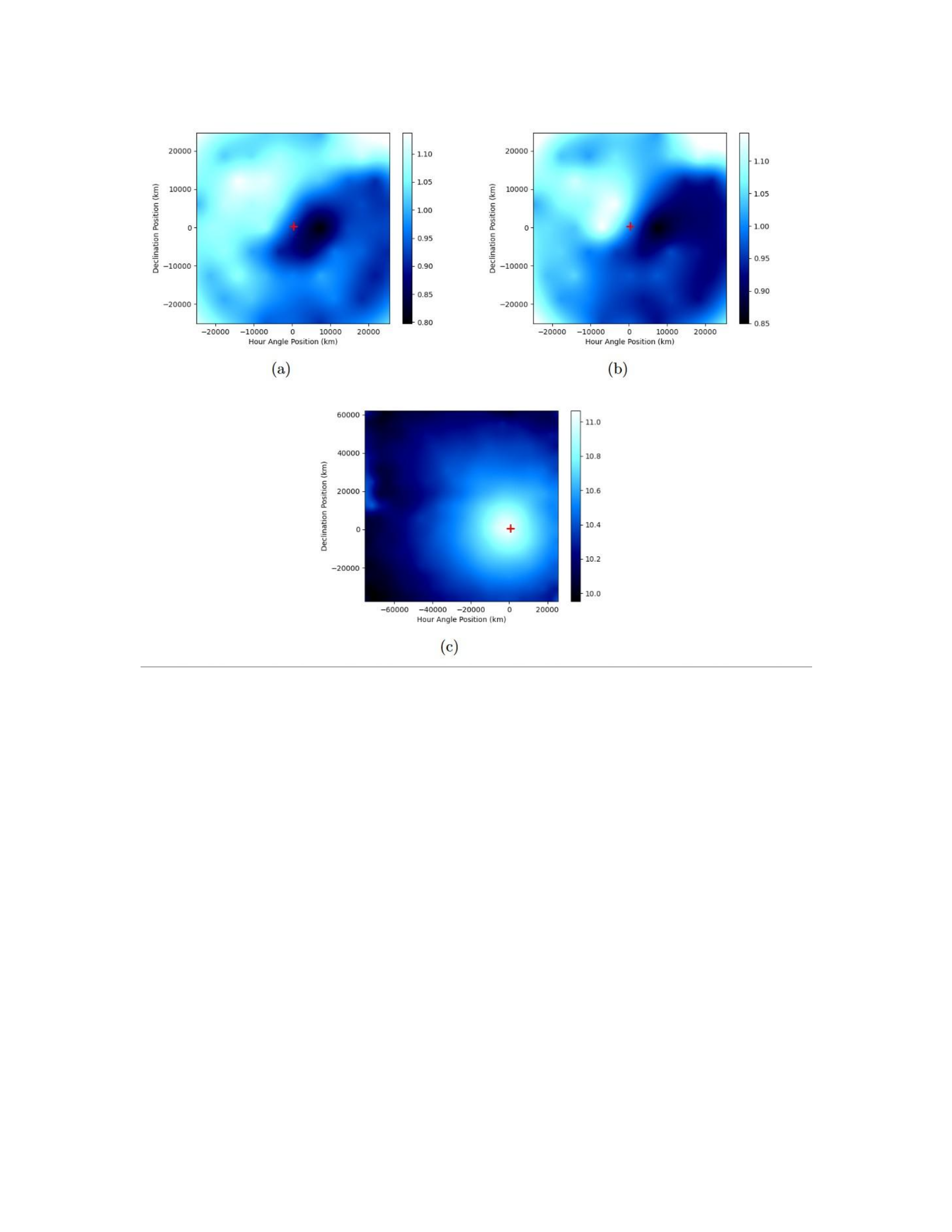
Carlo model [22]. Comparisons between the raw, azimuthal division, and radial division contour
plots are shown in
Figure 2.1 on the next page.
12
Figure 2.1
Sample IFU contour plots
Representations of the radially divided (a) and azimuthally divided (b) contour plots
(top) with their respective raw contour plot (bottom). Plots were of
𝐶
3 measurement
taken from Comet Garradd on 2011 August 22. The raw plot is slightly offset in terms
of the origin, as it is aligned with the optocenter (denoted by the red crosshair) of
the fiber array.
CHAPTER III
METHODS

13
There are no simple methods for analyzing the mechanical behavior of the comet, such as its
rotational motion, from the radical features expressed in the outer coma. We can, however, place
constraints on several parameters by simulation. A Monte Carlo model used by Schleicher and
Woodney [35] outlines a method by which we can use the properties of the detected dust
particles of our radical species and their motion over time to simulate the behavior of the features
found in our coma enhancement plots. Several parameters of the model can be adjusted
manually, and they are usually randomly generated within known boundaries. These include the
positions of the simulated active regions, the number and position of the particles within these
respective active regions, their outflow direction and velocity, and the rotational axis of the
comet, assuming no precession or nutation. Each run of the model will output several images
over a predetermined period of time that corresponds with the timespan of the comet
observations.
The model is used to simulate a variety of cases, with the parameters randomly varied
between each simulation [35]. The visual output of the model is then cross-referenced with the
comet enhancement plots by eye in order to determine a reasonable range of values for the
parameters. They are then adjusted slightly to yield a better overall fit of the simulated particles
with the features shown in the enhancement plots. With these determined physical parameters,
it is possible to constrain a rotational period for the comet.
3.1 The model
The outline for the Monte Carlo model involves generating a simplified, spherically symmetric
modelofthenucleusin3-dimensionalspace. Themodelmustbeinitializedwithseveralparameters

14
including pole orientation, latitudes and longitudes of jet features, outflow velocity of radical
particles, and a set rotational period. A fixed number of particles are generated within the 3D
space, on the order of 104. To determine if features in the outer coma are related to physical
active regions on the surface of the comet’s nucleus, we assume that they are the same quantity.
These particles represent dust grains from active regions of a spherically-symmetric nucleus. The
size of the comet nucleus is based on available literature for the target comet being studied.
Otherwise, if no published values exist, we work within a likely range of values for those comets.
The fraction of the nucleus that is considered active is determined by a pseudo-random number
generator operating within a range of 10 - 60%. The active fraction is constrained to one or more
regions with randomly generated sizes and positions on the nucleus, depending on how many
possible active regions can be determined from the enhancement plots. Particles that are located
within the boundaries of the active regions are sorted into a separate list from the ‘inactive’
particles, and are made visually distinct in the output plots via differing colors. A location for the
solar vector is set based on the comet’s orbital ephemeris at the time of observation. The chance
that a particle is released from the nucleus and emitted into the coma is determined by a
probability function of the cosine of the angle between the respective particle’s position and the
solar vector. If the particle is released from the nucleus, its outflow position and velocity are
tracked as it is emitted into the coma. The outflow dispersion angles for the particles are defined
by a random Gaussian distribution.
At the same time, the movement of the active regions due to the rotation of the comet is
simulated based on a predetermined rotational axis. For the sake of this model, a simple

15
rotational state is assumed, with no effects due to precession or nutation. Since the detected
features from our observations may not move at the same rate as the comet’s physical nucleus,
we cannot simply assume that our rotation parameter is the same value as the actual rotational
period.
Additional perturbations on the released particles exist in the form of solar radiation pressure.
For real comet dust grains, the pressure applied by radiation from the Sun has a non-negligible
effect. The pressure (in
𝑁
/
𝑚
2) on each particle can be determined by
𝐺𝑆𝐶
𝑟
®
𝑑
𝑃𝑟𝑎𝑑
=
𝐶𝑟𝑎𝑑
(3.1)
𝑐
| ®
𝑟𝑑
|3
where
𝐺𝑆𝐶
is the solar constant: 1361
𝑊
/
𝑚
2, and
𝑟
®
𝑑
is the displacement vector between each
particle and the Sun.
𝐶𝑟𝑎𝑑
is a constant where 2 corresponds to a perfectly reflecting surface, and
1 corresponds to perfect absorption. In reality, materials are neither totally reflecting nor
absorbing, so
𝐶𝑟𝑎𝑑
is randomly generated close to a value of 1, as dust grains tend to have low
albedos. The pressure is then multiplied by the cross-sectional area and divided by the mass for
each particle to determine the subsequent applied acceleration. For the scales of these particles,
we assume a mass on the range of 10−6 kg, and radii within a range of 0.1
𝜇
m to 1 mm [34]. A
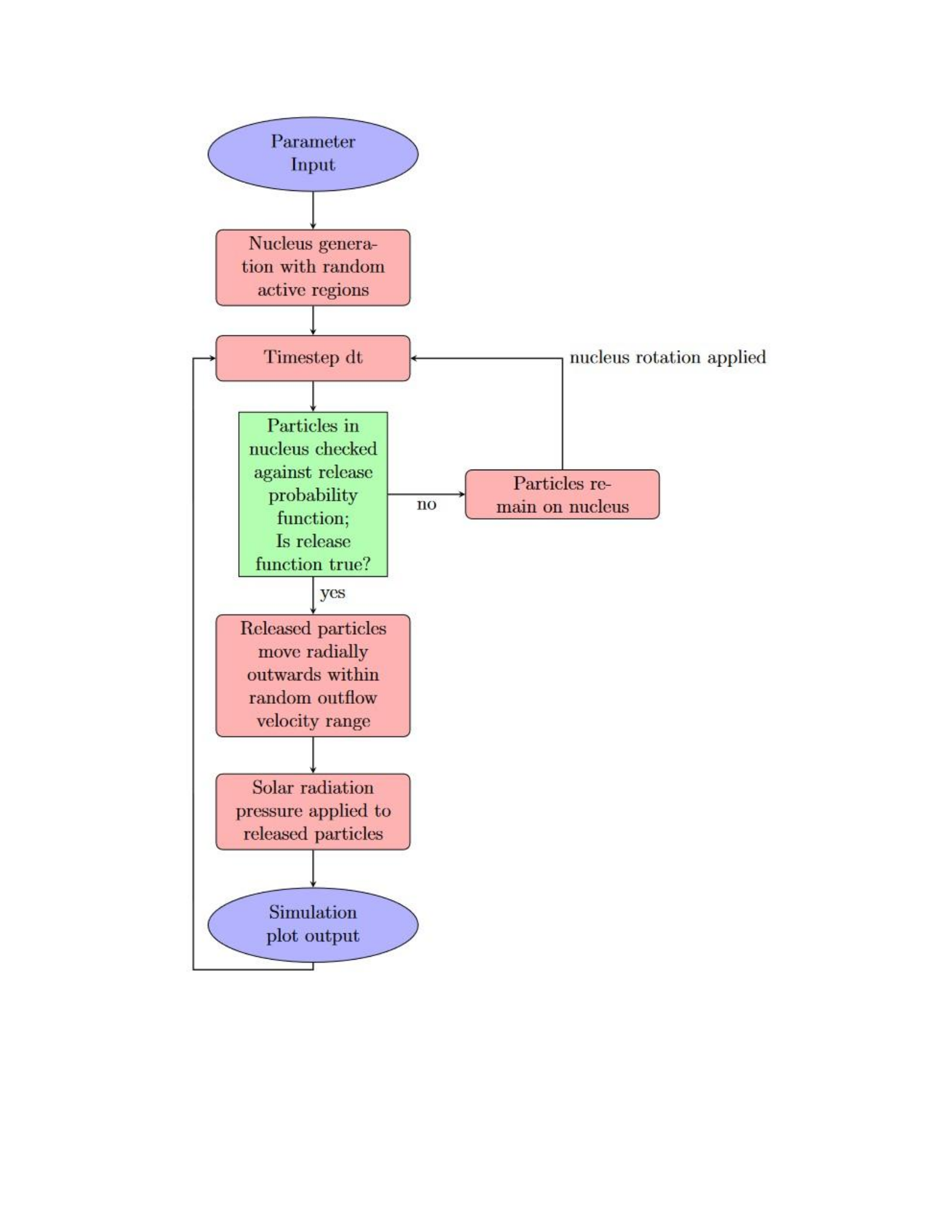
flowchart showing the step-by-step processes for the model is shown in Figure 3.1 on the
following page.
16
Figure 3.1 Flowchart for
model processes

17
3.2 Determining a limit for outflow velocity
One of the parameters that must be accounted for in the Monte Carlo model is the mean
outflow velocity of the radicals as they move outwards from the nucleus. Since there is no simple,
common factor amongst comets with regards to this behavior, we must try to determine it by
analyzing the positions of the emitted particles over time.
We use a similar method as [35] to constrain a velocity from our radial profile data. They
divided their enhanced division plots, obtained through narrowband photometry, into 10°
wedges, yielding 36 wedges in total. For each of these wedges that coincided with specific
morphological features in the coma, they examined the brightest points and tracked their relative
positions over the timespan of their observations. Due to the discrete, separated nature of our
fiber array spectrograph, as opposed to their CCD detector, we must use twelve 30° wedges to
ensure sufficient data are contained in each wedge. We tracked the radial position of the point
corresponding to the highest measured
𝑁𝑟𝑎𝑑
(where
𝑁𝑟𝑎𝑑
is the ratio between the column density
𝑁
and the modeled column density related to the projected radius from the optocenter,
𝑁𝑚𝑜𝑑𝑒𝑙
)
for constant features over the timespan of all of our observations for each night. The radial
positions for the carbon-bearing radicals, such as
𝐶
2 and
𝐶𝑁
, were grouped together to increase
the amount of available data.
These positions were plotted with respect to the difference in time from the first observation
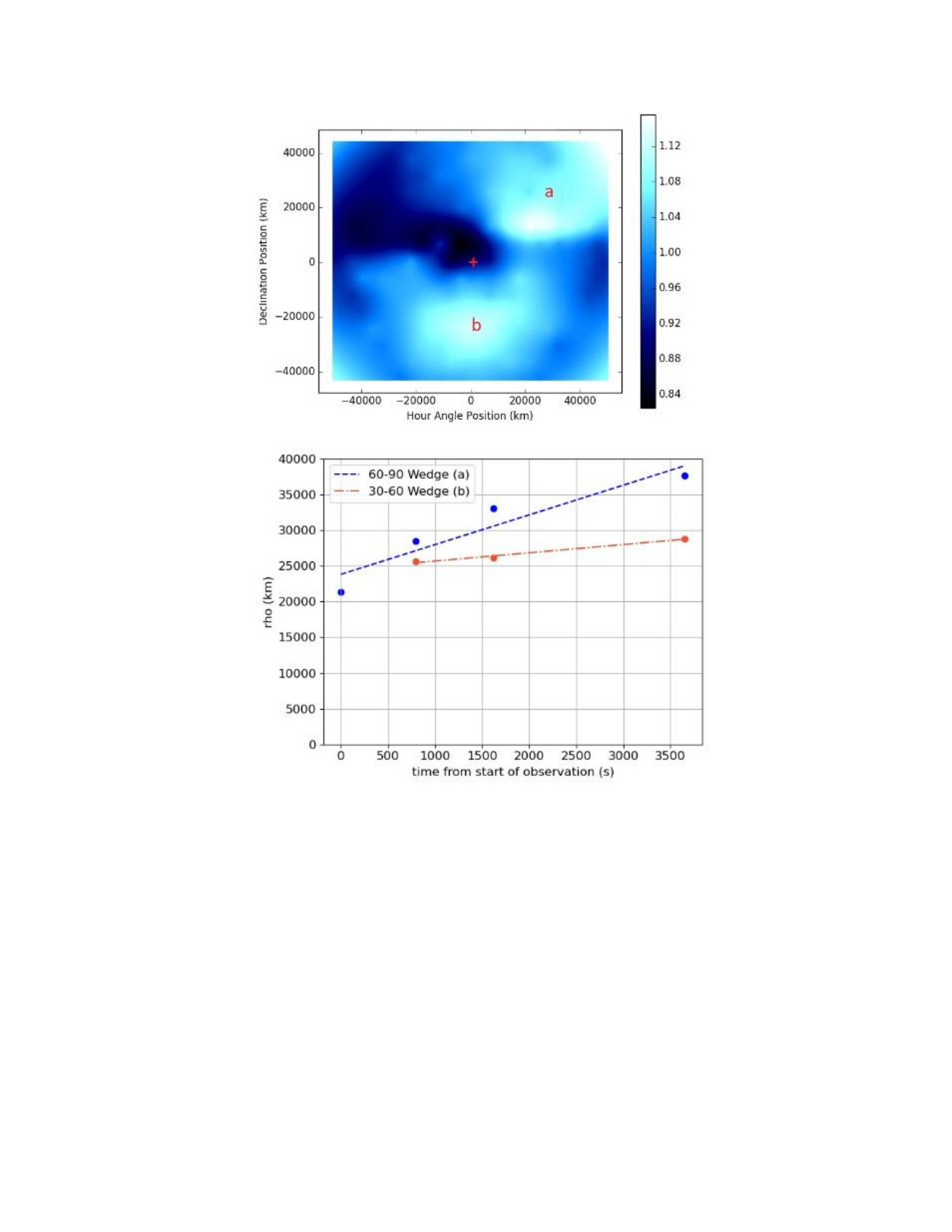
for each usable 30° wedge. A line of best fit was found for each using linear regression, as shown
in Figure 3.2 on page 19. By comparing the regression slope parameters of each wedge for each
night, we can determine an upper limit on the mean outflow velocity of the particles from the

18
nucleus. This, in turn, can be used as a parameter to better model the outflow behavior of the
particles in our Monte Carlo simulation. This process is repeated for each identified active region
in the comet’s coma.
As the dust particles get farther from the nucleus, forces such as solar radiation pressure and
gravity start to dominate [28]. These additional parameters must then be accounted for and
calculated based on each simulated particle’s relative position to the comet nucleus and the solar
angle.
19
Figure 3.2
Outflow feature angular positions
Angular positions of detected features over the timespan of the observations of
Comet Garradd. The above figure depicts an example
𝐶𝑁
radial division map, and
the bottom figure shows the position vs time relation for
𝐶𝑁
over all observations.
The color bar scale on the upper map represents the column density of
𝐶𝑁
. The blue
line of the bottom figure represents feature (a), while the orange line represents
feature (b)

20
3.3 Comparing spatial concentrations
While a qualitative method of visually comparing the model results with enhancement plots
was established, a more quantitative approach was desired as well. A method outlined by
Vaughan [39] for analysis of comet data from the same IFU spectrometer was utilized, where the
enhancement plots were divided into a circle with symmetrical 60° wedges, centered on the
optocenter fiber. The fibers that were located in these position angle wedges were used to
calculate the concentration
ratio Ω,
! !−1
𝐴𝑧𝑖𝐷𝑖𝑣
𝑅𝑎𝑑𝐷𝑖𝑣
1 1
Ω= + + (3.2)
𝜎
2
𝜎
2
𝜎
2
𝜎
2
𝐴𝑧𝑖𝐷𝑖𝑣
𝑅𝑎𝑑𝐷𝑖𝑣
𝐴𝑧𝑖𝐷𝑖𝑣
𝑅𝑎𝑑𝐷𝑖𝑣
where AziDiv and RadDiv correspond to the weighted averages of the azimuthal division values
and the radial division values, respectively, for each fiber. A larger number of fibers within each
wedge allows for more accurate values of Ω, which is why 60° wedges are used, as opposed to
the 30° wedges used in the outflow velocity determinations. If a fiber resides exactly on a line
dividing the wedges, the concentration values are determined from the weighted average of two
symmetric fibers along either boundary of the wedge.
!−1
∑︁
𝐴𝑧𝑖𝐷𝑖𝑣
1
𝐴𝑧𝑖𝐷𝑖𝑣
2
𝑅𝑎𝑑𝐷𝑖𝑣
1
𝑅𝑎𝑑𝐷𝑖𝑣
2
Ω= +
(3.3)
2 2 2 2 2
𝜎
𝜎
𝜎
𝜎
𝜎
𝐴𝑧𝑖𝐷𝑖𝑣
,1
𝐴𝑧𝑖𝐷𝑖𝑣
,2
𝑅𝑎𝑑𝐷𝑖𝑣
,1
𝑅𝑎𝑑𝐷𝑖𝑣
,2

21
where the summation term is
1 1 1
+ +
𝜎
2
𝜎
2
𝜎
2
𝐴𝑧𝑖𝐷𝑖𝑣
,1
𝐴𝑧𝑖𝐷𝑖𝑣
,2
𝑅𝑎𝑑𝐷𝑖𝑣
,1
𝑅𝑎𝑑𝐷𝑖𝑣
,2
The average Ω values are then calculated for each wedge for each moment of observation.
The Ω
𝑎𝑣𝑔
values for each comet and observation are shown in Appendix A. This method is known
as
Welch’s Analysis of Variance (ANOVA).
Since the model does not simulate discrete fibers, the concentration is simply determined by
dividing the final output into 60° wedges and calculating the ratio of the number of particles in
each wedge with the overall total particles produced for the simulated comet nucleus. With
concentration values organized in this way, we now have an additional method of comparing the
model results with our observed enhancement plots after they have been initially constrained by
eye.

22
CHAPTER IV
RESULTS
The rotation of the comet is accounted for by setting a principal axis of rotation and including
a parameter for a change in angular position for set time-step intervals. Each time-step of the
model corresponds to the observations from the IFU spectrograph. For each time-step, the
particles within the active regions are checked against the release probability function. If they
pass the check, they are emitted radially outwards from the nucleus. If they do not pass, the
particle remains on the nucleus as it rotates in each interval. This process is repeated for every
time-step, with the emitted particles continuing their outward motion based on the outflow
velocity values. Non-released particles have a chance to pass the release probability check with
every step.
The outputs from the three-dimensional model are manually analyzed in a two-dimensional
grid to compare with the observable features as seen on the plane of the sky in the 2-D contour
plots. The rotational period of our coma model was adjusted until we were able to approximate
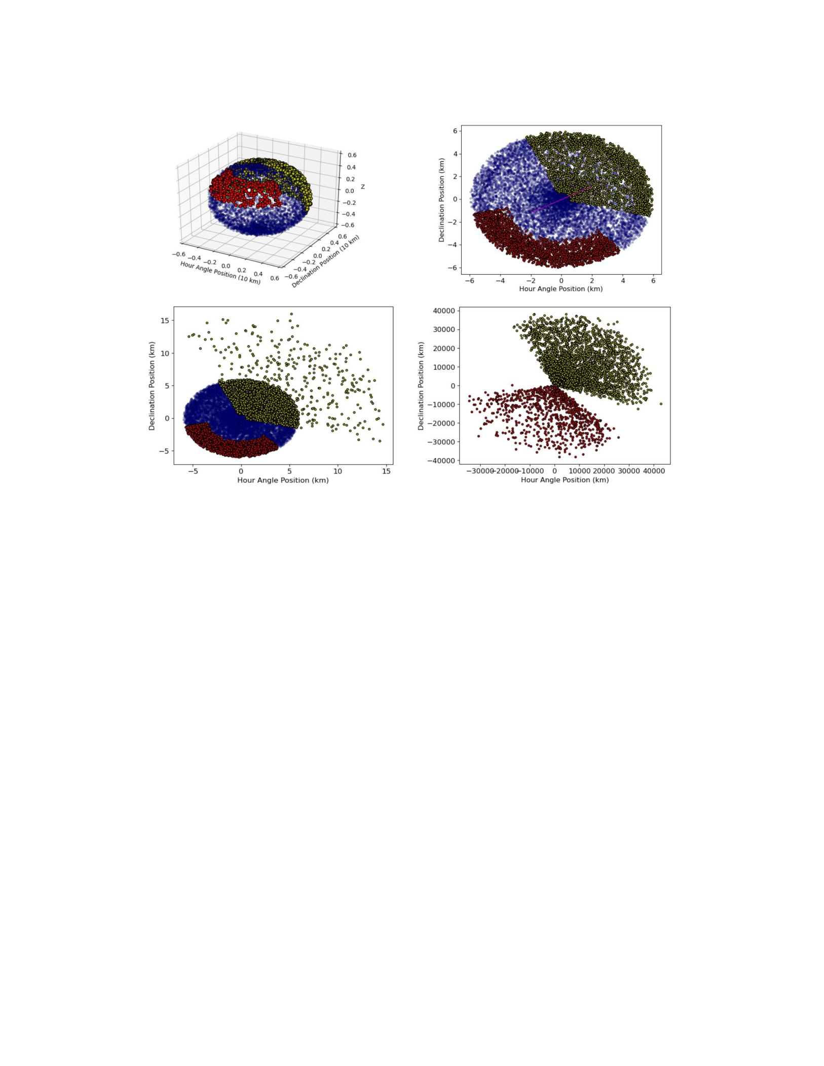
an acceptable fit to our observations obtained with the IFU. A sample output of the model is
shown in
Figure 4.1 on the following page.
23
Figure 4.1
Sample nucleus of model
The top left image shows an initial setup in three dimensions, while the figure on the
top right depicts the respective setup in two dimensions, with the z-axis increasing
out of the page as the nucleus would be seen on the plane of the sky. The colored
circles represent the modeled particles. Inactive particles are blue, and the separate
active regions are shown in red and yellow. The two-dimensional plots are primarily
used to compare our results with the IFU observations. The bottom figures
represents subsequent timesteps.
4.1 10P/Tempel 2
Comet 10P/Tempel 2 is a Jupiter-family comet that was observed with the IFU spectrograph.
Tempel 2 has been a subject of much analysis from outside sources [23], making it a useful body
for comparison. The effective radius of the nucleus was determined to be 5.98 ± 0.04 km [24],
which is very large for a JFC. The rotation period was determined to be 8.950 ± 0.002 hours by

24
Knight et al. [21] at the time of its 2010/2011 perihelion approach. Furthermore, the period was
also determined to have increased slightly between perihelion passages in 1988 and 1999,
possibly due to systematic torque [23].
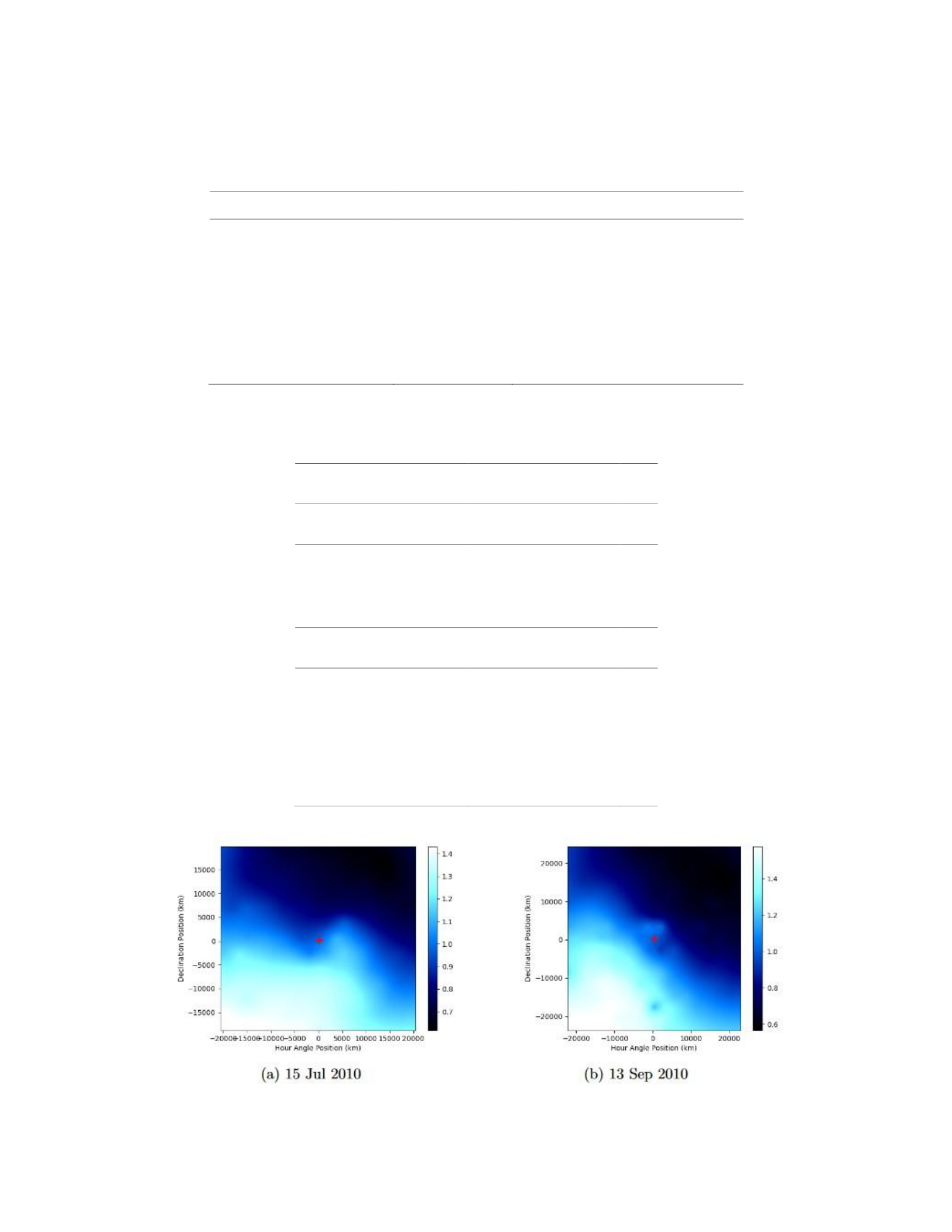
From our radial division maps for the carbon-bearing radicals of Tempel 2, we were able to
determine one large primary feature in the coma, as shown in Figure 4.2 on page 27. This area of
high column density was present in our observations from 2010 July 15 and September 13,
suggesting they are from the same active source. The angular position of the feature changes
very little between observations taken on each date, suggesting that the active region from which
it originates is located near a rotational pole. A similar feature was observed from the
𝑁𝐻
2 radial
division maps, though it is smaller in size.
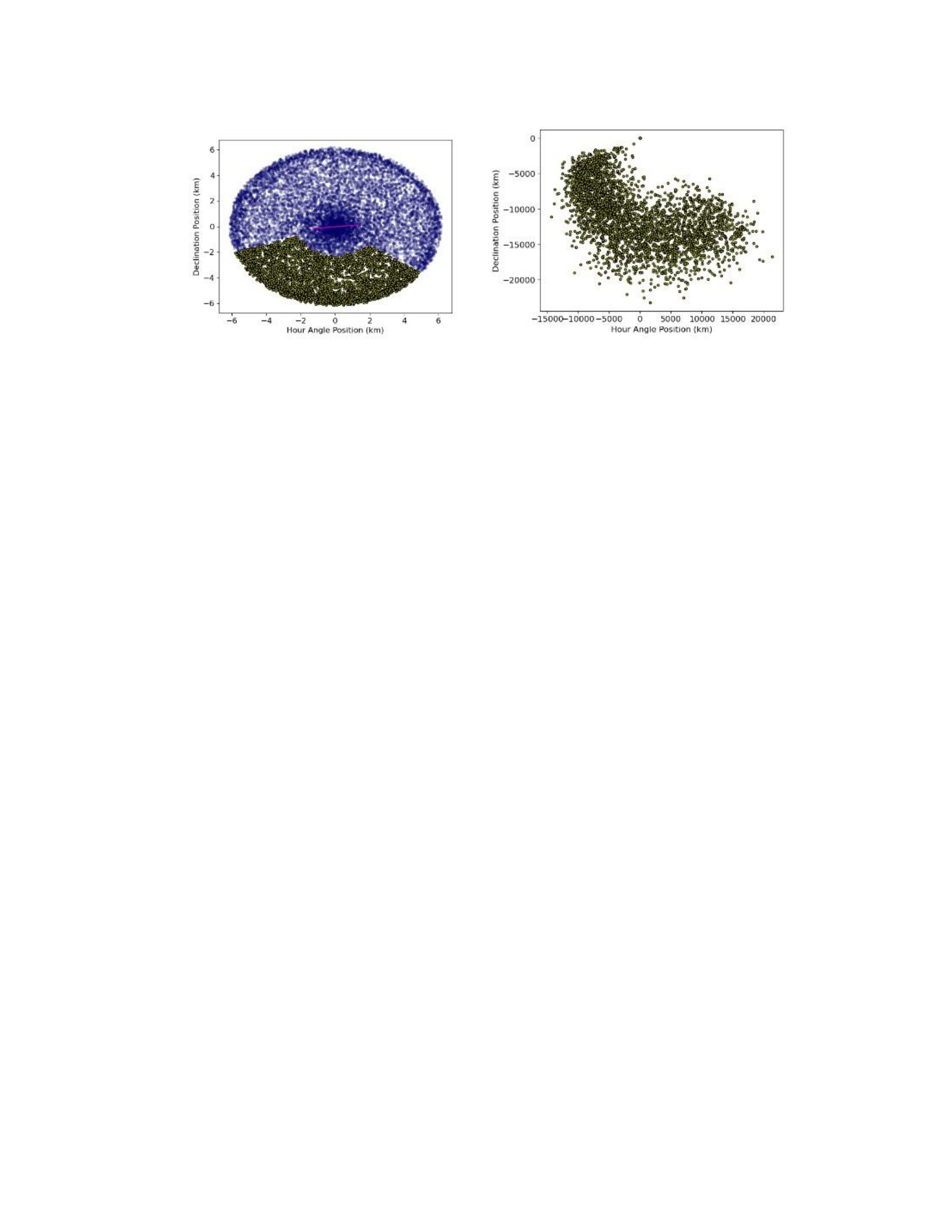
Our Monte Carlo model was constrained to see if similar conditions could be observed from
the output. Thirty cases were produced from a parameter range, and the best fit was visually
chosen from among them. The parameters used for the final Tempel 2 simulations are shown in
Table 4.1 on page 26. The resulting images are shown in Figure 4.3 on page 28
Tempel 2 illustrates one of the main limitations with our model: working with a small number
of observations. Tempel 2 was observed with the IFU spectrograph for only two nights, both with
a small temporal range. Observation times are detailed in Table 4.2 on page 26. As comet
rotational periods tend to be at least several hours long, the available observations only offer a
glimpse at the spatial behavior for comparison with the simulation results. Furthermore, coma
plots from each enhancement date show only a single feature for all radical species, limiting our
ability to constrain our simulated plots by our usual visual standards.
25
Table 4.1
Tempel 2 Model Parameters
Parameter Name
Value
Source
Radius
6 km
Lamy & Toth et al. 2009 [24]
Outflow velocity
0.6 km/s
Knight et al. 2012 [23]
Solar Vector Angle
109°
NASA Horizons
Rotation period
8 ± 0.5 hours
Custom parameter output
Active Area Fraction
34.3 ± .01 %
Random parameter output
Number of test cases
30
Result
Table 4.2
Observation times for Tempel 2
Observation Label
Start Time (UTC)
July 15 2010
278
08:39
300
279
08:48
600
280
09:03
900
September 13 2010
400
09:08
600
401
09:22
900
402
09:39
900
407
11:08
900
408
11:25
600

26
Figure 4.2
Radial division maps for
𝐶𝑁
in Tempel 2
ThelargeactivefeaturecanbeseeninthelowerleftinboththeJuly(left)andSeptember
(right) observations, suggesting little dynamic activity in this period of the comet’s orbit.
27
Figure 4.3
Plots for Comet Tempel 2 from the Monte Carlo model
The first image shows one of the earliest time-steps for the simulation, while the last
shows the resultant plot after a simulated passage of a little over 8 hours. The purple
line running through the nucleus in the left plot denotes the simulated primary
rotation axis, which is partially perpendicular to the plane of the figure.
4.2 C/2009 P1 (Garradd)
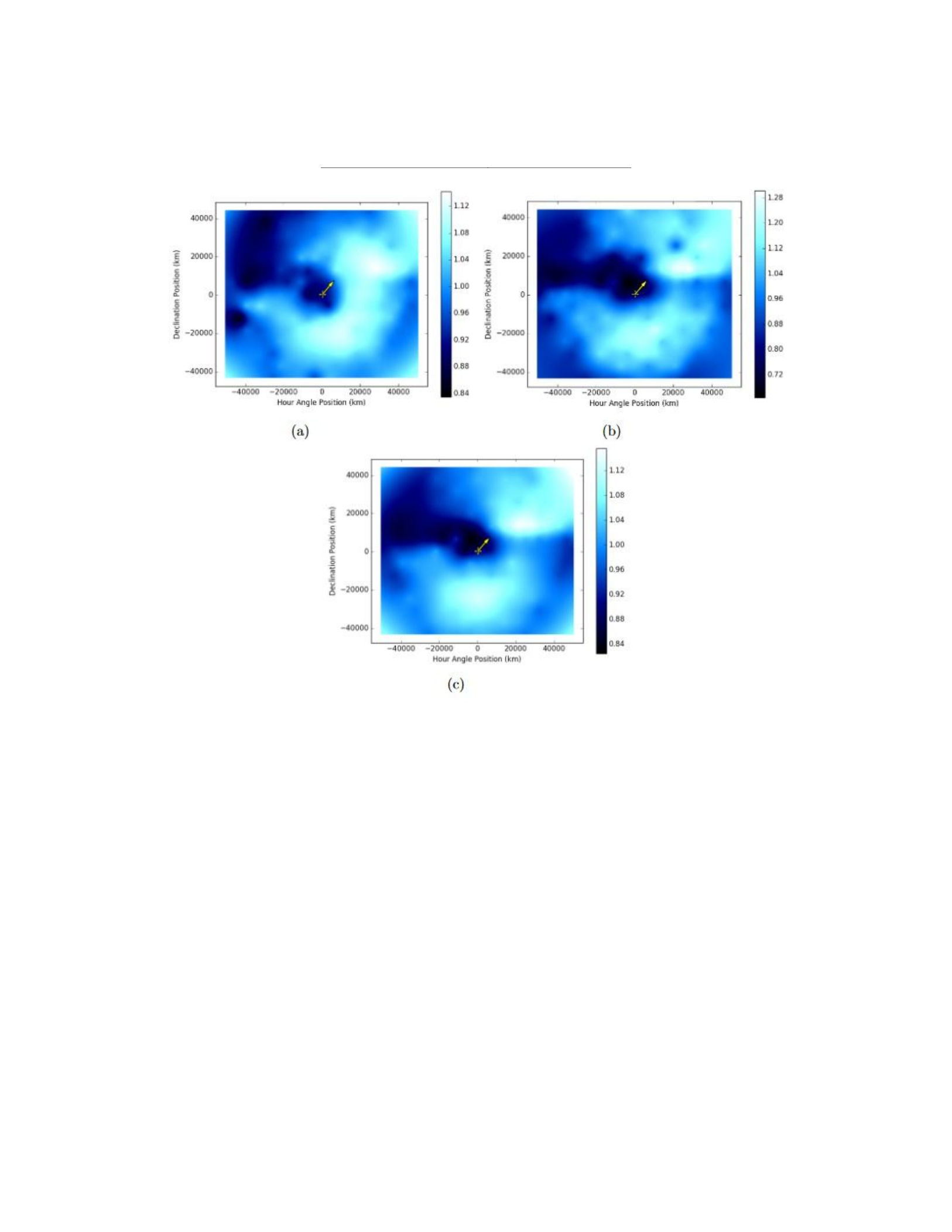
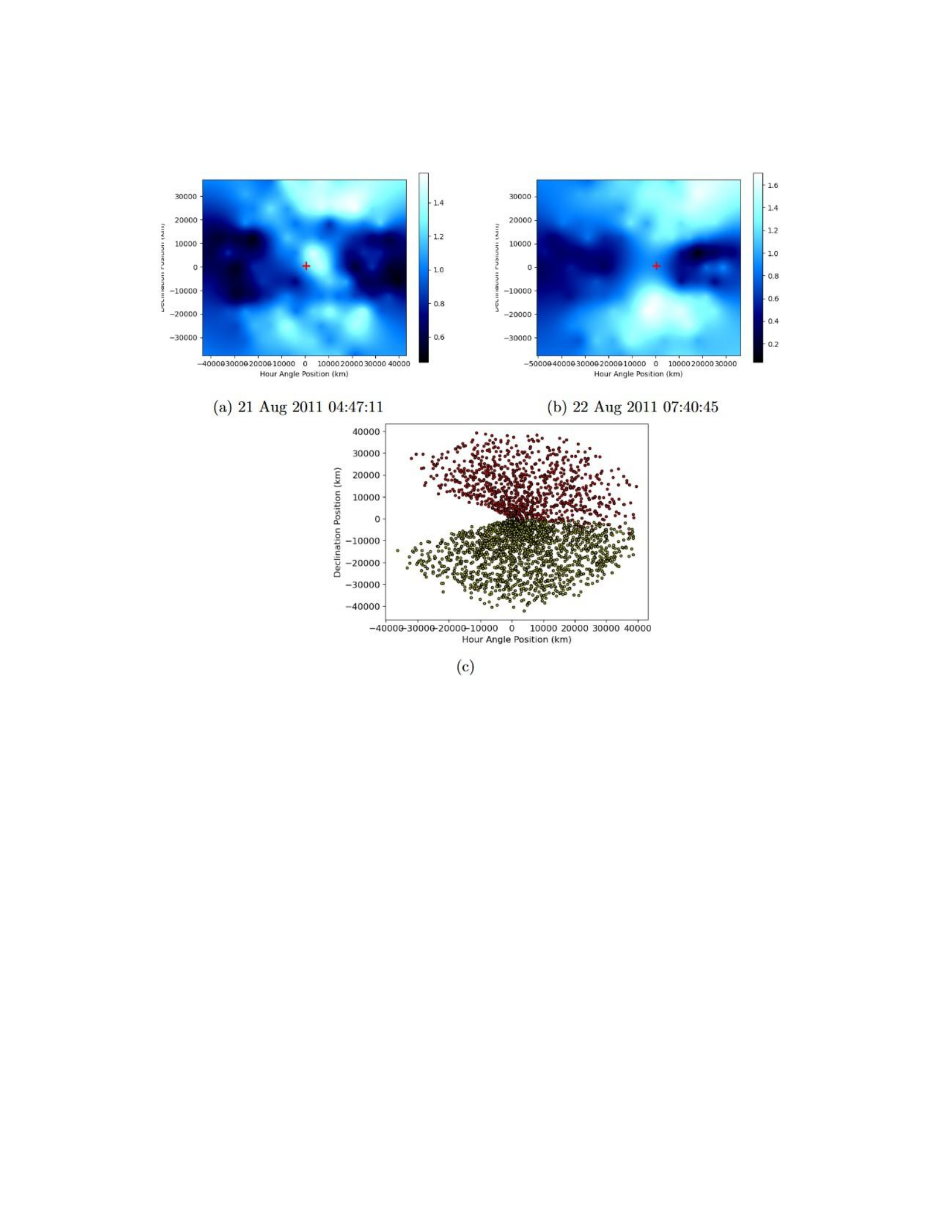
Our observations of comet Garradd showed a continuous feature present in the upper right
quadrant of the division maps for the carbon-bearing radicals, as seen in Figure 4.4 on page 32.
This suggests a relatively simple rotational mode for the comet, with the feature possibly
originating near the pole of the primary rotational axis. As such, we first tested our simulation by
inputting parameters from Garradd that were observed and also supported by other sources.
These are given in Table 4.3 on page 31. Due to the appearance of two features, a wider test case
of about seventy runs was required for a best-match simulation. Observation times are shown in
Table 4.4 on page 31, with each observation having a 600 second duration.
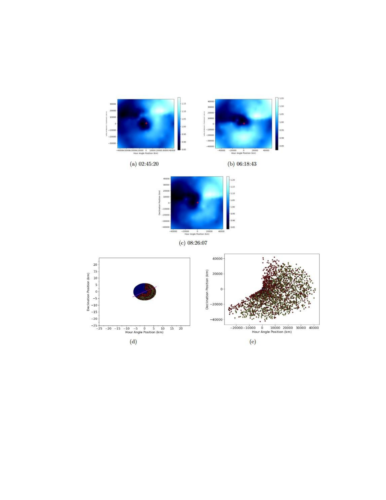
Figure 4.5 on page 34 shows comparisons between sample radial division plots and model
simulation results that most visually resemble them. The simulated total active area fraction was
generated as 49.5%, which would support our estimate that Garradd is a highly active comet. The

28
water production rates measured by Boissier et al. [6] suggests an active area fraction of at least
50%. One notable distinction from the model output is the lower concenctration of particles in
the feature in the bottom of the map for Figure 4.5b. This can be due to limitations with the
model, or it could indicate a more complex rotational mode for Garradd than was initially
assumed, as the feature is not present for the entire night of observations. It could also be due
to the fact that the simulated nucleus is stationary, with the only motion being due to rotation.
In reality, the comet is travelling through space as it orbits the Sun, so if an active jet were to
rotate away from view, we wouldn’t still be seeing all the residual outflow. All the carbon-bearing
radicals appear to have similar morphologies over our observation period, suggesting they
originate from the same source regions on the surface of the nucleus.
𝐶𝑁
is typically chosen for
primary visual comparison, as it has a better contrast in the coma compared to the other radicals
due to the strength of the violet band [23].
The concentration ratio of the active particles in the simulation shown in Figure 4.5 on page
34 match the Welch’s ANOVA wedge concentration spread, with the 0°, 240°, and 300° wedges
having the most activity across both. There is a difference in that the 0°-60° wedge in the model
has a slightly higher concentration than the 240°-300° wedge (27.5% and 28%, respectively) while
the relationship is reversed in the ANOVA concentrations found for
𝐶𝑁
, as shown in Appendix A.

29
Table 4.3
Comet Garradd Model Parameters
Parameter Name
Value
Source
Radius
5.6 km
Boissier et al. 2013 [6]
Outflow velocity
1-25 m/s
Mazzotta et al. 2016 [29]
Solar Vector Angle
139°
NASA Horizons
Rotation period
8 hours
Custom parameter
Active Area Fraction
49.5%
Random parameter
Primary Rotation Axis
𝜋
/6
Random Parameter
Number of test cases
75
Result
Table 4.4
Observation times for 2009/P1 Garradd
Observation Label
Start Time (UTC)
August 21 2011
944
02:45
946
03:12
948
03:46
950
04:16
952
04:47
958
06:18
960
06:50
962
07:21
964
07:53
966
08:26
968
08:59
August 22 2011
1028
02:53
1029
03:08
1034
04:34
1035
04:46
1039
05:52
1042
06:35
1046
07:40
30
1051
09:01
1054
09:39
Figure 4.4
Radial division maps for Comet Garradd
Observations taken on the night of 2011 August 21 at 06:18 local time. The color bars
represent the column density of the detected radical. The white feature that can be
seen in the upper right is present for most of the night’s observations. This suggests
an active region rich in carbon-based molecules. The small yellow crosses represent
the locations of the optocenter, and the arrows represent the direction of the solar
vector. The solar vectors are pointing mostly out of the screen. The maps depict
𝐶
2,
𝐶
3, and
𝐶𝑁
, respectively.
While the spatial distributions of the carbon-bearing radicals are very similar to each other,

31
𝑁𝐻
2 exhibits a very different outgassing behavior for Garradd. Two coma features can be seen
opposite to each other on the top and bottom parts of the enhancement plots, similar in
appearance to an hourglass. This indicates that the features originate from two separate sources,
with the bottom source being different than the active region responsible for the carbon-bearing
radicals. These plots and their respective model simulation comparisons are shown in Figure 4.6
on page 35. The active particle spread most matches the ANOVA concentrations of the August 22
observations, with the wedges in the 60°-120° and 240°-360° regions showing the highest density
(14.4%, 24.2%, and 25.7%, respectively).
Both the
𝑁𝐻
2 and
𝐶𝑁
simulations had the same generating parameters, showing how they
could have separate morphology and possible source regions and yet arise from the same
rotational state. The model simulated a timespan of 292 hours with timesteps of 300 seconds.
Our best comparison plots were produced from an initial parameter for rotation period of 8 ± 0.5
hours. This is lower than values obtained from other authors. Farnham et al. [12] determined a
value of
10.4 ± 0.05 hours from lightcurve measurements, while Ivanova et al. [18] determined a period
of 11.1 ± 0.8 hours using a cross-correlation method of tracking a morphological feature over
time, similar to our own. Due to the wider number of available usable observations for Comet
Garradd, an additional method for checking the period was done by determining our own
lightcurve from the enhanced plots. The phase determined from this method also corresponded
with a period of 8±0.75 hours, which agrees with our model result. This suggests that this value
is at least consistent with our own observations. The lightcurve is shown in Figure 4.7 on page
32
36. The discrepancy of our results from the others determined may be due to our different
observation methodology.
Figure 4.5
Garradd model CN comparison
Comparisons between radial division maps for
𝐶𝑁
in Comet Garradd and simulated
maps from the Monte Carlo model. The top three images show results over the night
of 2011 August 21 and their respective observation timestamps. The bottom row
shows maps randomly generated by the model that appear visually closest to the
enhancement plots, with the left being the initial generated nucleus and the right
33
being the result after several timesteps. The purple line running through the nucleus
in the left plot denotes the simulated primary rotation axis.
Figure 4.6
Garradd model NH2 comparison
Comparisons between radial division maps for
𝑁𝐻
2 in Comet Garradd and simulated
maps from the Monte Carlo model. The top images show a sample observation over
two different nights. The bottom row shows a map randomly generated by the model
that appear visually closest to the enhancement plots.

34
Figure 4.7
Garradd enhancement plot lightcurve
Lightcurve determined from our enhancement plots for our observations taken over
two nights. The blue dot represent observations taken on August 21, red dots
represent August 22. A phase (gray sine curve) was determined from similar
morphological features found in the enhancements of all radicals across both nights.
4.3 168P/Hergenrother
Comet Hergenrother presented unique challenges compared to our other comets. It is
another Jupiter Family Comet, whereas Garradd is a long-period comet, and thus likely has
different physical properties in terms of nucleus size and active area fraction, and a lot less is
known about Hergenrother as opposed to the other comets in this study. In terms of radicals,
Hergenrother was found to be extremely chemically depleted [33], allowing only viable
observations for
𝐶𝑁
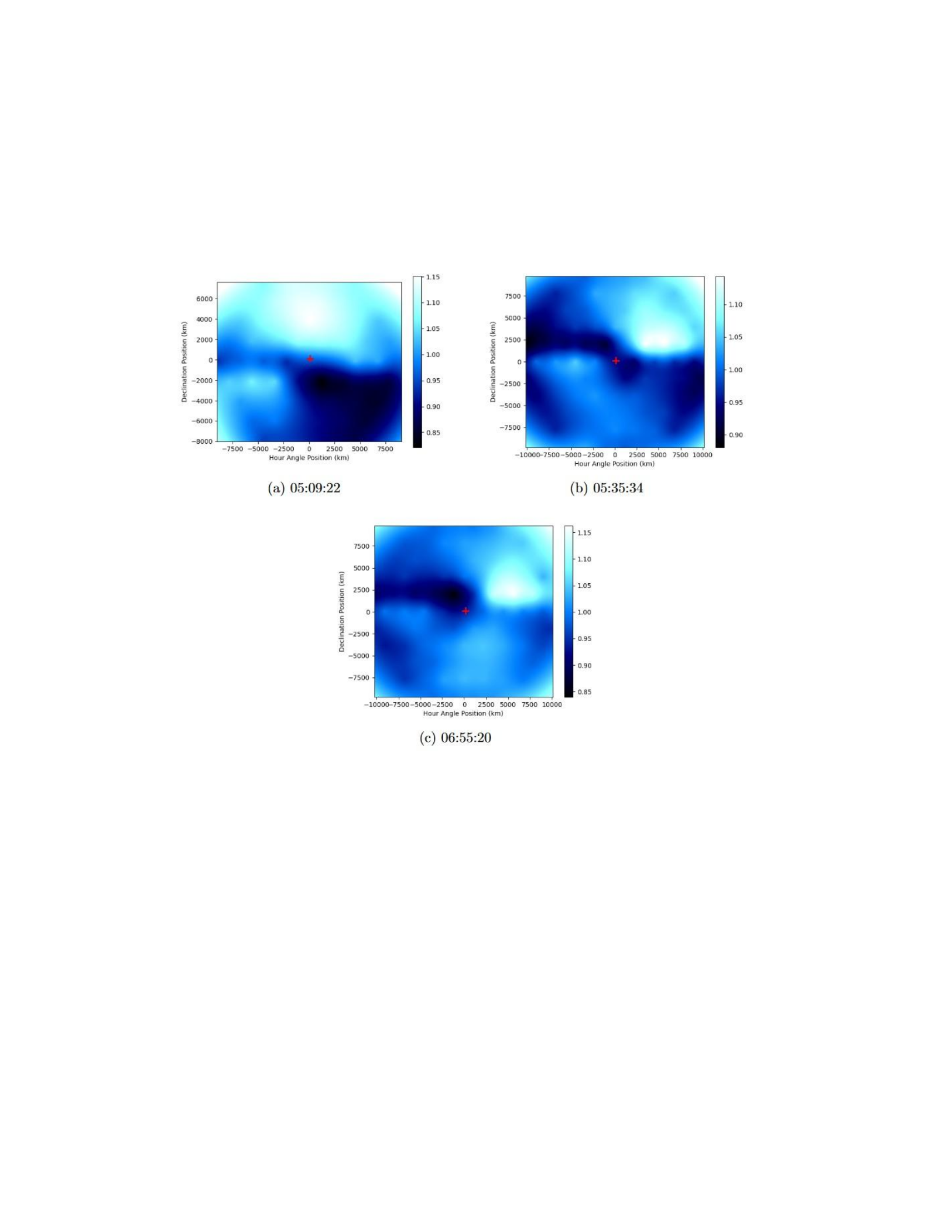
. Only one bright feature can be seen in the
𝐶𝑁
maps, shown in Figure 4.8 on
page 41, so only one active area was set in the model. Fifty runs were required for Hergenrother

35
as well. The closest visual simulations are achieved by setting a rotation period parameter of 6.5
hours, and are shown in
Figure 4.9 on page 42. The other model parameters are shown in Table 4.5 on the following page.

36
Table 4.5 Comet Hergenrother Model
Parameters
Parameter Name
Value
Source
Radius
0.7 km
Custom
parameter
Outflow velocity
1-15 m/s
Custom
parameter
Solar Vector Angle
159°
NASA Horizons
Rotation period
6.5 ± 0.5 hours
Custom
parameter
Active Area Fraction
19.4 ± .01%
Random
parameter
Number of test cases
50
Result
Table 4.6 Observation times for
168P/Hergenrother
Observation Label
Start Time (UTC)
October 06 2012
1200
05:09
1201
05:35
1202
06:00
1203
06:55
1204
07:18
October 08
1307
02:57
1308
03:20
1309
03:42
1310
04:06
1314
05:39
1315
06:02
1320
08:01
October 09
1372
02:20
1373
02:44
1377
04:18

37
1378
04:42
1381
05:53
1384
07:01
1389
08:55
December 19 2012
1423
01:14
1424
01:48
December 20
1514
06:43
December 21
1577
01:15
1578
01:47
The active area fraction for the surface of the nucleus was 19.4 ± 0.01% for this best-match
simulation. This is much lower than the best-match runs for Garradd, which coincides with our
observation that Hergenrother is chemically depleted and less active compared to most comets
[33]. It remains to be seen if the depletion of Hergenrother, or its recent lack of detection near
its last expected perihelion [41], are related to the aforementioned fragmentation event. The
model constrainstherotationperiodforouranalysisof168Pto6.5±0.5hours.
Therearenomeasurements of Hergenrother’s rotation period from outside sources with which to
compare our result.
Due to the aforementioned chemical depletion, Welch’s ANOVA wedge comparisons were
done with our measurements of
𝐶𝑁
. The simulation output yield concentrations in the 0°-60°,
60°-120°, and 300°-360° wedges of 36.1%, 32%, and 28.5%, respectively. The actual ANOVA
calculations show higher wedge concentrations primarily in the 0°-60°, 240°-300°, and 300°-360°
regions, differing slightly from our model. This indicates that our model results may not align to
38
our observations with high precision. It is difficult to further constrain, as almost half of our
Hergenrother observations were dominated by a low signal-to-noise ratio, which can affect the
amount of usable fibers in the ANOVA calculations.
Figure 4.8
Hergenrother maps
𝐶𝑁
radial division maps for Comet Hergenrother on the night of 2012 October 6. Due
to the small interval of time coverage of the observations shown, the singular bright
feature in the upper right of each map moves very little between images.
39
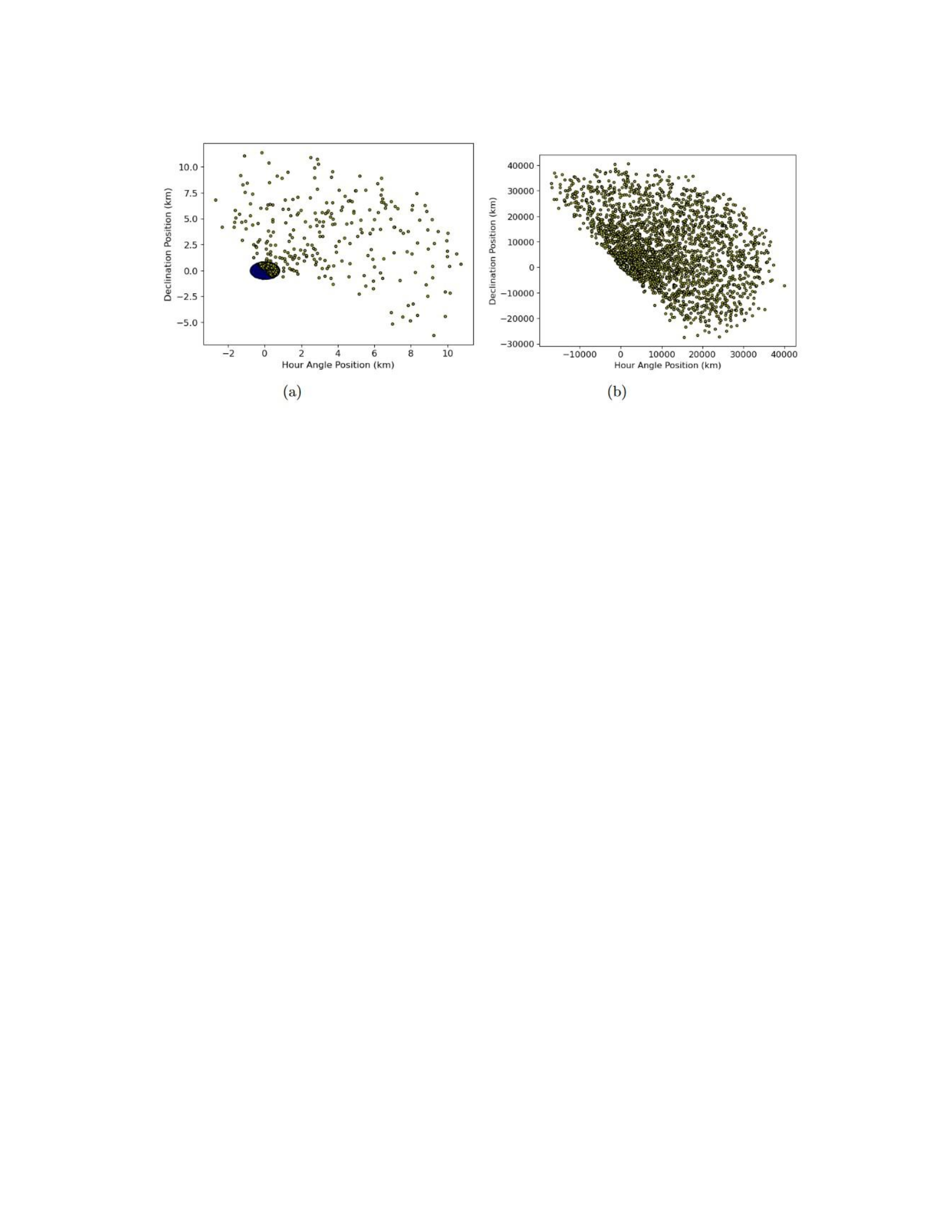
Figure 4.9
Hergenrother model CN comparison
Plots for Comet Hergenrother from the Monte Carlo model. The first image shows
one of the earliest time-steps for the simulation, while the last shows the resultant
plot after a simulated passage of about 290 hours. The purple line running through
the nucleus in the left plot denotes the simulated primary rotation axis.
CHAPTER V
CONCLUSION AND FUTURE WORK
The rotational period parameters that were set for the best-matching model results for each
comet were very close to the period constrained by either other sources or by visually tracking
the periods over multiple observations. The model also simulates possible active area fractions
for the comets and their approximate locations on the surface. These parameters are not well
constrained by observation alone, so these values can be of interest to other parties. The values
determined for active area fractions (34%, 50%, and 19% for Tempel 2, Garradd, and
Hergenrother respectively) suggests that long period comets like Garradd have higher active area

40
fractions than JFC’s such as Tempel 2 and Hergenrother, as they have experienced more
outgassing and perihelion passages.
Other methods of visually inferring rotational states of comets involves working with data
taken via multiple observations over a long timespan, typically months apart. The data for our
comets were only collected over a couple concurrent nights by the George and Cynthia Mitchell
IFU Spectrograph, limiting the long-term comparisons that could be done with our model. As
such our model results are only effective as comparisons with specific “snapshots" of the comets’
behavior. Further constraints could be placed with further observations, especially comparing
preand post-perihelion activity.
Future efforts will be spent on improving the model. Dust and gas are two very different
components of comet composition and exhibit different outflow behavior, especially beyond the
first few kilometers after release from the nucleus. Our reduced division maps from the IFU
spectrograph are based primarily on the gas located in the outer coma, and we must be cautious
in establishing a link to the dust outflow from the nucleus generated by the Monte Carlo model.
While both may come from similar jet sources, gasinteractions typically require parent-daughter
molecule interactions. A possible method of improvement would be to implement techniques
from a similar Monte Carlo model by Lederer et al. [25], in which trajectories of parent molecules
are tracked, and possible daughter decays are simulated by a exponential decay function. The
daughter molecules are ejected isotropically from the parent, and both are subsequently tracked
vectorially in the coma [25]. Additionally, the current version of the Monte Carlo model only
accounts for simple rotation around a primary axis. A more realistic model can be attempted by

41
accounting for more complex rotational states, such as precession and nutation, that have been
observed for other comets, such as Hartley 2 [4]. The comet’s translational motion as it moves
along its orbital path around the Sun could also be considered to eliminate residual outflow
between timesteps. Further checks must also be made to ensure uniqueness of our model
simulations, as multiple three-dimensional configurations of active area locations could
theoretically produce visually similar two-dimensional plots. The parameters of the model can be
adjusted accordingly as more information on our comets is corroborated and published by
outside sources.
CHAPTER I
INTRODUCTION
Scientists across multiple fields, not just physics and astronomy, have an interest in comets
and their connection to the formation of the solar system. Many questions concerning the
chemical and biological evolution of life on Earth involve the early conditions of the planet.
Accretion of material in the outer distances of the solar system led to the formation of comets.
Initially postulated as “dirty snowballs” [40], recent observations of the composition of comets
led astronomers to view them more as “icy dirtballs”, consisting mainly of ice, rock, and organic
compounds that coalesced
togetherintolowdensitystructuresduringtheearlyageofthesolarsystem, over4.5billionyearsago
[3]. Thiscompositionappearstoholdtrueevenforobservedinsterstellarcomets, suchas2I/Borisov
[8], which was observed passing through our solar system in 2019. Comets are usually grouped

42
by their orbital characteristics, with the longer-period comets originating from distant small-body
populations such as the Kuiper Belt, the scattered disk, and the Oort Cloud. The existence of these
populations support a model of the evolution of the solar system known as the Nice model,
where the gas giants were in more cicular, closely spaced orbits at the edge of the inner disk.
Small icy bodies were scattered by the gas giants inwards, which caused Saturn, Uranus, and
Neptune to migrate outwards due to conservation of angular momentum [38]. Further
interactions with Jupiter caused the icy bodies to enter highly elliptical orbits, while Jupiter
migrated slighty inwards towards its current postion. An alternative model known as the grand
tack hypothesis proposes that Jupiter instead initially migrated inwards from a distance of 30 AU
and then outwards after capturing Saturn in a mean-motion resonance [26]. This hypothesis has
developed more recent support from studies of comets C/2014 S3 (PANSTARRS) and
67P/Churyamov-Gerasimenko, where the low detection of collisional elements in these outer
bodies corresponds with the early migration of Jupiter and Saturn posited in the grand tack [37].
Comets tend to be less dynamically active and exhibit less change in volatile composition
compared to other major bodies in the solar system. Thus, they provide insight into the physical
and chemical properties of the early conditions of the solar system. Insitu measurements of
comets, such as the Stardust mission, have detected organic molecules, including the amino acid
glycine [9]. Such evidence supports the hypothesis that comets were key to delivering the
precursors to life to early Earth. However, recent studies into comets, including the Rosetta
mission, have measured the Deuterium-to-Hydrogen (D/H) ratio, which was determined to be at
least three times greater than the ratio for the Vienna Standard Mean Ocean Water (VSMOW) on

43
Earth, (1.5576±0.0001)×10−4 [27]. This suggests the opposite to the long-held idea that comets
were also the means through which water came to our planet. Cometary science is still rapidly
changing and can still provide much in the way of constraints of the formation of Earth and the
solar system.
The majority of comets fall within two categories: short-period and long-period comets, based
on whether their orbital revolution periods are less than, or greater than, 200 years. Most short
period comets, known as Jupiter-family comets (JFCs), are theorized to have originated from
beyond Neptune, in the scattered disk of the Kuiper Belt region. They tend to orbit in the same
ecliptic plane as the planets and have periods of less than 200 years. The exception to these are
the Halley-family comets. While they also have a short orbital period, they are highly inclined to
the ecliptic, suggesting a different region of origin: the distant Oort Cloud. Proposed by Jan Oort
in 1950, the Oort Cloud is a theoretical, spherical region of space dominated by icy planetesimals
that were theorized to have formed during the same time period as the planets [32] [10]. Long-
period comets by contrast are highly eccentric, leading to orbital periods that range from
hundreds to thousands of years. These long-period comets are also thought to have originated
from the Oort Cloud. As many have hyperbolic trajectories, long-period comets will only have a
single solar apparition before they escape the solar system.
Due to their possible connection to the formation of the solar system, comets are the subject
of numerous chemical surveys [15]. Narrow-band photometry [1] and spectroscopic surveys [7]
have shown that the majority of comets are similar in chemical composition, with the exception
that a significant fraction of JFCs are depleted in carbon-chain molecules. Observations of the

44
dust-to-gas ratio and the abundances of carbon-based radical species (
𝐶𝑁
,
𝐶
3,
𝐶
2, etc.) show little
correlation based on composition or dynamical family. The subtle variances exhibited in the
comets based on their classes suggest differences in dynamical evolution rather than different
conditions of formation [7].
Due to the nature of comets, many properties have to be inferred from the types of radiation
we can detect remotely, as in situ observations are a rare opportunity. One such property is the
rotational period of the comet, which has most commonly been determined from the measured
lightcurve. If a celestial target such as a comet is observed over a long enough period, it is possible
to graph the flux or intensity of the measured light over time. If periodicity is seen in the
lightcurve, then it is possible to determine a spin period of the nucleus. Further constraints could
be made if multiple lightcurves are made over a range of heliocentric distances, as was made
with 1P/Halley [14]. Active areas are determined from spherical nucleus approximations, even
though they tend to be elliptical in nature. Constraints are made based on the size and flux of
emission sources, and are determined as fractions of the surface area of the nucleus [20].
1.1 Target comets
The comets examined in this research were C/2009 P1 (Garradd), Comet 168P/Hergenrother,
and Comet 10P/Tempel 2. Garradd was an active, dynamically young, long-period comet at the
time of observation, likely making its first trip through the solar system. The comet is in a highly
eccentric orbit of e = 1.001, and has an inclination of 106.18 degrees. Comet Hergenrother is a
Jupiter-family comet with an orbital period of about 6.90 years. It has an orbital eccentricity e =

45
0.610, and an inclination of 21.93 degrees. Tempel 2 is also a JFC, with e = 0.5363, an inclination
of 12.02 degrees, and an orbital period of about 5.5 years.
Comet Garradd was very active during its pre-perihelion transit, with one of the highest dust-
to-gas ratios and water production rates observed in a comet [5]. The
𝐶𝑂
2/
𝐻
2
𝑂
and
𝐶𝑂
/
𝐻
2
𝑂
ratios were measured from September-October 2011, and in January-March 2012, and were
found to be less abundant post-perihelion [5]. Since the ices in comets are primarily composed
of these volatiles, we can determine how the activity is driven during the comet’s passage. An
asymmetry between the two ratios from pre- to post-perihelion also suggests either a large-scale
chemical heterogeneity in the nucleus [30], or that the rotational state led to an effect where one
hemisphere was exposed to more activity from solar exposure than the other [13]. It also had a
high active surface area to nucleus area ratio.
Comet Hergenrother was a recently discovered comet, of which few publications exist. It
underwent an outburst in 2012, which may have resulted in a fragmentation event a few weeks
afterward and has been reported as overdue for its 2019 apparition after it was not detected
near its expected perihelion passage. [41]. Pierce and Cochran [33] performed spectroscopic
analysis of Hergenrother and found it to be the most depleted comet reported in
𝐶
2,
𝐶
3, and
𝑁𝐻
2.
Observations of such events can provide unique insight into the chemical and physical properties
of comets during a period of high activity. Fragments of Comet 73P/Schwassmann-Wachmann 3
were observed to have similar chemical properties but physical heterogeneities [16]. The
fragmentation event itself can also affect the dust production, such as with C/1994 S4 LINEAR [2],
or the orbital parameters, as with the Kreutz sungrazers, a family of comets believed to have

46
originated from a common progenitor comet that fragmented into two parts during a past
perihelion approach within 3.45 solar radii [19]. These super-fragments were then believed to
have undergone their own fragmentation events upon subsequent perihelion passages [36].
In contrast, 10P/Tempel 2 has been extensively studied since its discovery in 1873. Its short
orbital period, allowing for multiple observations over dozens of apparitions, as well as it once
being a possible target for a flyby mission, has made it the object of numerous ground-based
studies. Its next close approach to Earth is due to occur in August 2026 with a nominal geocentric
distance of 0.41 AU. It has been observed to have low outgassing activity and brightness pre-
perihelion, and has a typical dust-to-gas ratio of other comets with a similar perihelion distance
[23].
CHAPTER II
OBSERVATIONS
Observations of comets primarily focus on two components: the nucleus and the coma. The
nucleus corresponds to the solid part of the comet. Nuclei are typically comprised of dust and
ice, and tend to have a size range on the order of a few to tens of kilometers. As the nucleus is
exposed to heat from the Sun, the ices trapped on or below the surface can sublimate. The
resultant atmosphere of gas surrounding the nucleus is known as the coma. As the comet
approaches the Sun, the visible coma can increase in size to an order of tens of thousands of
kilometers in diameter, as ice grains can continue to sublimate as they’re dragged outwards by
the gas. Due to the low albedo and smaller size of the nucleus compared to the coma, direct

47
observations of the nucleus are usually restricted to in situ measurements. For comets Garradd
and Hergenrother, the measurements for this study were taken of their respective comae from
ground-based telescopic observations. The observations for Comet Garradd were obtained pre-
perihelion, while the Hergenrother and Tempel 2 observations were obtained post-perihelion.
Specific observation and calibration parameters for Garradd, Hergenrother, and Tempel 2 are
shown in Table 2.1 and Table 2.2 on page 8.
ThecomaobservationswereobtainedwiththeGeorgeandCynthiaMitchellSpectrograph. This
integral-field unit (IFU) spectrograph is a low- to moderate- resolution fiber optic spectrograph
consisting of 246 optical fibers. The optical fibers each have a diameter of 4.1 arcsec and are
arranged in a 1.7 x 1.7 arcmin array, alternating from 14 to 15 bundled fibers per row [17]. A
diffraction grating covered the passband from 3600-5800 Å and provides a spectral resolving
power (
𝜆
/Δ
𝜆
) of 850. The spectrometer was used in conjunction with the 2.7 m Harlan J. Smith
Telescope located at McDonald Observatory in Fort Davis, Texas. In order to maintain the comet’s
position on the array, a tracking star is used with a fiducial that moves opposite to the comet’s
motion. Any star spectra caught crossing through the field of view are removed in analysis [33].
Observations were taken of various radical species with spectral emission bands visible in
the spectrometer’s passband, including
𝐶
2,
𝐶
3,
𝐶𝐻
,
𝐶𝑁
, and
𝑁𝐻
2. Each fiber in the array was
connected to a charge-coupled device (CCD) and yield independent spectra. The raw data were
initially reduced through bias subtraction, flat fielding, and calibration in flux and wavelength.
Since the measured spectra are a mix of the emission bands from the coma superposed on a
continuum from the reflection of the solar spectrum off the dust in the coma, analogue stars

48
were utulized. Each night the flux and color of a solar analog star is matched with the observed
comet’s spectrum, and the solar spectrum is subsequently removed.
Table 2.1
Comet Observation Parameters
Comet
Obs. Date
r
𝐻
1
Δ2
Phase Angle3
Pre/Post
(UT)
(AU)
(AU)
(Degrees)
Perihelion
10P/Tempel 2
2010 Jul 15
1.43
0.72
42.2°
Post
2010 Sep 13
1.60
0.67
21.8°
Post
C/2009 P1 (Garradd)
2011 Aug 20
2.28
1.40
16.1°
Pre
2011 Aug 21
2.27
1.39
16.4°
Pre
2011 Aug 22
2.26
1.39
16.9°
Pre
168P/Hergenrother
2012 Oct 6
1.42
0.44
14.8°
Post
2012 Oct 8
1.42
0.44
16.1°
Post
2012 Oct 9
1.42
0.44
16.7°
Post
2012 Dec 19
1.66
0.99
32.7°
Post
2012 Dec 20
1.66
0.99
32.7°
Post
2012 Dec 21
1.67
1.00
32.7°
Post
Table 2.2
Comet Calibration Targets
Comet
Obs. Date (UT)
Flux Standard
Solar Analogue
10P/Tempel 2
2010 Jul 15
Feige 98
None
2010 Sep 13
BD+25 3941
HD 191854
C/2009 P1 (Garradd)
2011 Aug 20
BD+25 3941
39 Tau
2011 Aug 21
Feige 15
HD 6204
2011 Aug 22
BD+28 4211
HIP 109931
168P/Hergenrother
2012 Oct 6
Feige 15
HD 19518
2012 Oct 8
BD+28 4211
HIP 109931

49
2012 Oct 9
BD+28 4211
16 Cyg B
2012 Dec 19
Feige 15
Hyades 64
2012 Dec 20
Feige 34, Feige 56
35 Leo
2012 Dec 21
Feige 15, Feige 25
Hyades 64, HD19518
The reduced data were separated into columns representing the fiber number, the base-10
logarithm of the projected distance from the comet nucleus (
𝑙𝑜𝑔
(
𝜌
)), the logarithm of the column
density of the respective radical (
𝑙𝑜𝑔
(
𝑁
)), and the
𝑥
and
𝑦
coordinates of the coma measurement
from the comet nucleus. For the Garradd and Hergenrother data,
𝑥
corresponded to the hour
angle offset in kilometers, and
𝑦
corresponded to the declination position in kilometers. The
radial distance from the comet nucleus,
𝜌
, was determined by the distance formula
√︃
𝜌
=
𝑥
2 +
𝑦
2 (2.1)
The optocenter fiber was determined from each observation from the fiber corresponding to the
lowest value of
𝜌
. This single fiber is designated as the position of the comet nucleus.
Raw contour plots were generated for each observation, with the variables corresponding to
the
𝑥
and
𝑦
values for each observation, and the contour levels corresponding to the
𝑙𝑜𝑔
(
𝑁
) values.
The data were then analyzed based on their arrangement about the optocenter. In order to model
enhanced coma features as a function of projected distance from the nucleus, azimuthal rings
were determined based on the fibers being arranged in concentric, hexagonal rings about the
optocenter.
For each pixel in the ring, the projected distance was measured from the optocenter by

50
√︃
|
𝜌
−
𝜌
0| = (
𝑥
−
𝑥
0)2 + (
𝑦
−
𝑦
0)2 (2.2)
where
𝑥
0 and
𝑦
0 representthehorizontalandverticalpositionoftheoptocenter,and
𝑥
and
𝑦
represent
the horizontal and vertical position of the respective pixel. For each pixel in each azimuthal ring,
the values for |
𝜌
−
𝜌
0| were averaged, yielding an averaged radius value (
𝜌𝑎𝑣𝑔
). The column
densities for each fiber in the ring were also averaged, yielding an azimuthally averaged column
density value
𝑁𝑎𝑣𝑔
. In order to describe the relationship of the column density of each radical
with respect to the projected distance from the nucleus, a relationship
𝑁𝑚𝑜𝑑𝑒𝑙
was determined,
𝑁𝑚𝑜𝑑𝑒𝑙
=
𝐶
|
𝜌
−
𝜌
0|
𝑘
, (2.3)
where
𝐶
and
𝑘
are constants determined from a weighted least-squares fit. The fit parameters
were determined from the linear relation
log(
𝑁𝑚𝑜𝑑𝑒𝑙
) =
𝑘
log(|
𝜌
−
𝜌
0|) + log(
𝐶
) (2.4)
To further examine the heterogeneities of the radicals, azimuthal division coma enhancement
plots were generated, with the contour levels corresponding to the column density
𝑁
of each
fiber divided by the respective
𝑁𝑎𝑣𝑔
of the azimuthal ring. Radial division coma enhancement
plots were generated in a similar manner, with the contour levels corresponding to the ratio of
𝑁
over
𝑁𝑚𝑜𝑑𝑒𝑙
for each fiber in the array.
These azimuthal and radial coma enhancements can be used to look for coma features such
as jets or arcs. In addition to comparing coma features for each radical species across different

51
comets, they can also be used to observe how these features change over time. By focusing on
how the features change in position over several observations, we can attempt to link coma
features with changes in the physical nucleus, and recurring coma morphological features can be
used to constrain possible rotational states of the comets. The most common way to constrain
comet rotation periods is through analyzing a measured lightcurve to look for periodic, repeating
behavior [31]. A technique similar to ours used by Esterle [11] with Comet Halley involves
dynamically modeling simulated dust jets about the long axis mode of the comet nucleus over
time, and comparing them with jets seen in ground-based observations. Comparing
spectroscopic features allows for an additional method of analyzing rotation by use of a Monte
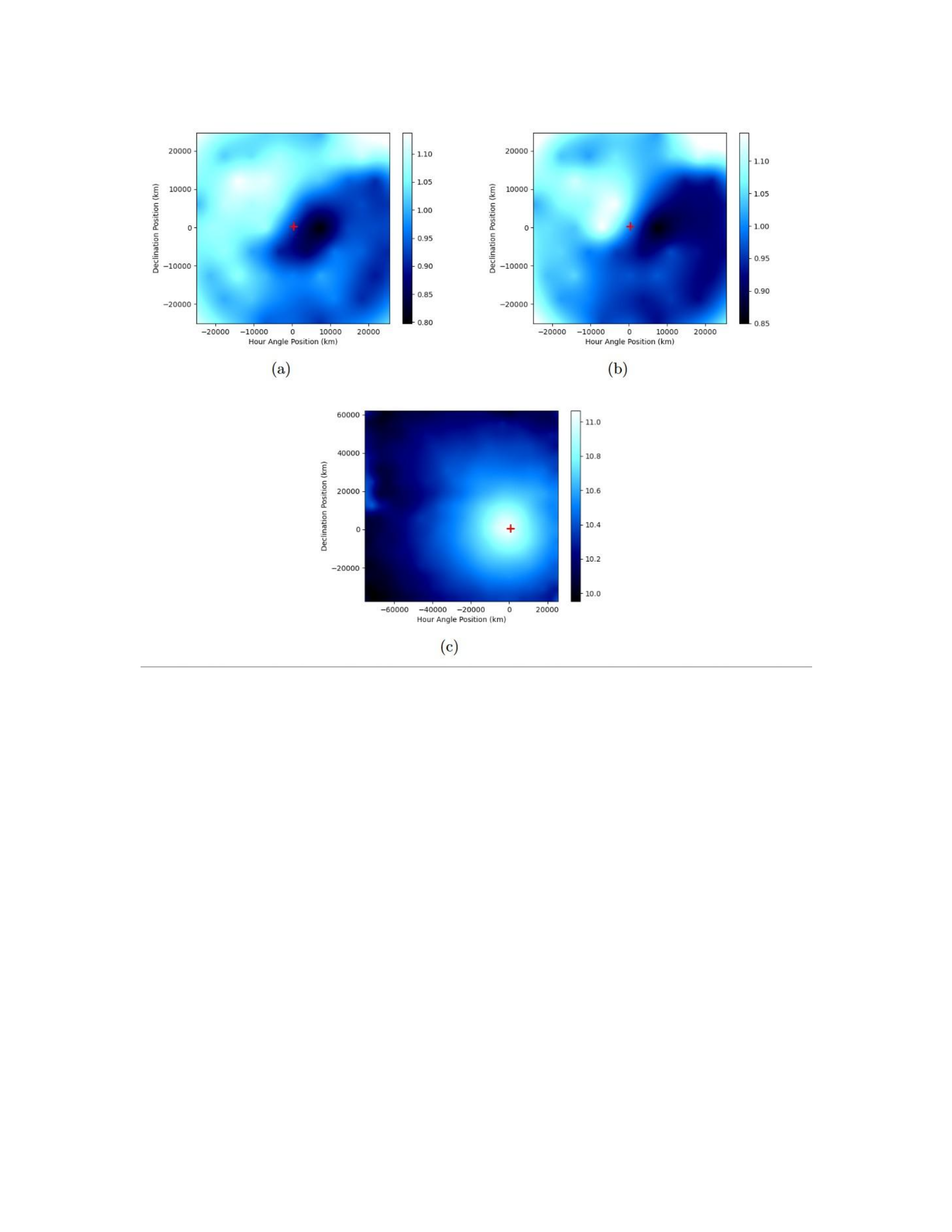
Carlo model [22]. Comparisons between the raw, azimuthal division, and radial division contour
plots are shown in
Figure 2.1 on the next page.
52
Figure 2.1
Sample IFU contour plots
Representations of the radially divided (a) and azimuthally divided (b) contour plots
(top) with their respective raw contour plot (bottom). Plots were of
𝐶
3 measurement
taken from Comet Garradd on 2011 August 22. The raw plot is slightly offset in terms
of the origin, as it is aligned with the optocenter (denoted by the red crosshair) of
the fiber array.
CHAPTER III
METHODS

53
There are no simple methods for analyzing the mechanical behavior of the comet, such as its
rotational motion, from the radical features expressed in the outer coma. We can, however, place
constraints on several parameters by simulation. A Monte Carlo model used by Schleicher and
Woodney [35] outlines a method by which we can use the properties of the detected dust
particles of our radical species and their motion over time to simulate the behavior of the features
found in our coma enhancement plots. Several parameters of the model can be adjusted
manually, and they are usually randomly generated within known boundaries. These include the
positions of the simulated active regions, the number and position of the particles within these
respective active regions, their outflow direction and velocity, and the rotational axis of the
comet, assuming no precession or nutation. Each run of the model will output several images
over a predetermined period of time that corresponds with the timespan of the comet
observations.
The model is used to simulate a variety of cases, with the parameters randomly varied
between each simulation [35]. The visual output of the model is then cross-referenced with the
comet enhancement plots by eye in order to determine a reasonable range of values for the
parameters. They are then adjusted slightly to yield a better overall fit of the simulated particles
with the features shown in the enhancement plots. With these determined physical parameters,
it is possible to constrain a rotational period for the comet.
3.1 The model
The outline for the Monte Carlo model involves generating a simplified, spherically symmetric
modelofthenucleusin3-dimensionalspace. Themodelmustbeinitializedwithseveralparameters

54
including pole orientation, latitudes and longitudes of jet features, outflow velocity of radical
particles, and a set rotational period. A fixed number of particles are generated within the 3D
space, on the order of 104. To determine if features in the outer coma are related to physical
active regions on the surface of the comet’s nucleus, we assume that they are the same quantity.
These particles represent dust grains from active regions of a spherically-symmetric nucleus. The
size of the comet nucleus is based on available literature for the target comet being studied.
Otherwise, if no published values exist, we work within a likely range of values for those comets.
The fraction of the nucleus that is considered active is determined by a pseudo-random number
generator operating within a range of 10 - 60%. The active fraction is constrained to one or more
regions with randomly generated sizes and positions on the nucleus, depending on how many
possible active regions can be determined from the enhancement plots. Particles that are located
within the boundaries of the active regions are sorted into a separate list from the ‘inactive’
particles, and are made visually distinct in the output plots via differing colors. A location for the
solar vector is set based on the comet’s orbital ephemeris at the time of observation. The chance
that a particle is released from the nucleus and emitted into the coma is determined by a
probability function of the cosine of the angle between the respective particle’s position and the
solar vector. If the particle is released from the nucleus, its outflow position and velocity are
tracked as it is emitted into the coma. The outflow dispersion angles for the particles are defined
by a random Gaussian distribution.
At the same time, the movement of the active regions due to the rotation of the comet is
simulated based on a predetermined rotational axis. For the sake of this model, a simple

55
rotational state is assumed, with no effects due to precession or nutation. Since the detected
features from our observations may not move at the same rate as the comet’s physical nucleus,
we cannot simply assume that our rotation parameter is the same value as the actual rotational
period.
Additional perturbations on the released particles exist in the form of solar radiation pressure.
For real comet dust grains, the pressure applied by radiation from the Sun has a non-negligible
effect. The pressure (in
𝑁
/
𝑚
2) on each particle can be determined by
𝐺𝑆𝐶
𝑟
®
𝑑
𝑃𝑟𝑎𝑑
=
𝐶𝑟𝑎𝑑
(3.1)
𝑐
| ®
𝑟𝑑
|3
where
𝐺𝑆𝐶
is the solar constant: 1361
𝑊
/
𝑚
2, and
𝑟
®
𝑑
is the displacement vector between each
particle and the Sun.
𝐶𝑟𝑎𝑑
is a constant where 2 corresponds to a perfectly reflecting surface, and
1 corresponds to perfect absorption. In reality, materials are neither totally reflecting nor
absorbing, so
𝐶𝑟𝑎𝑑
is randomly generated close to a value of 1, as dust grains tend to have low
albedos. The pressure is then multiplied by the cross-sectional area and divided by the mass for
each particle to determine the subsequent applied acceleration. For the scales of these particles,
we assume a mass on the range of 10−6 kg, and radii within a range of 0.1
𝜇
m to 1 mm [34]. A
flowchart showing the step-by-step processes for the model is shown in Figure 3.1 on the
following page.

56
Figure 3.1 Flowchart for
model processes

57
3.2 Determining a limit for outflow velocity
One of the parameters that must be accounted for in the Monte Carlo model is the mean
outflow velocity of the radicals as they move outwards from the nucleus. Since there is no simple,
common factor amongst comets with regards to this behavior, we must try to determine it by
analyzing the positions of the emitted particles over time.
We use a similar method as [35] to constrain a velocity from our radial profile data. They
divided their enhanced division plots, obtained through narrowband photometry, into 10°
wedges, yielding 36 wedges in total. For each of these wedges that coincided with specific
morphological features in the coma, they examined the brightest points and tracked their relative
positions over the timespan of their observations. Due to the discrete, separated nature of our
fiber array spectrograph, as opposed to their CCD detector, we must use twelve 30° wedges to
ensure sufficient data are contained in each wedge. We tracked the radial position of the point
corresponding to the highest measured
𝑁𝑟𝑎𝑑
(where
𝑁𝑟𝑎𝑑
is the ratio between the column density
𝑁
and the modeled column density related to the projected radius from the optocenter,
𝑁𝑚𝑜𝑑𝑒𝑙
)
for constant features over the timespan of all of our observations for each night. The radial
positions for the carbon-bearing radicals, such as
𝐶
2 and
𝐶𝑁
, were grouped together to increase
the amount of available data.
These positions were plotted with respect to the difference in time from the first observation
for each usable 30° wedge. A line of best fit was found for each using linear regression, as shown
in Figure 3.2 on page 19. By comparing the regression slope parameters of each wedge for each
night, we can determine an upper limit on the mean outflow velocity of the particles from the

58
nucleus. This, in turn, can be used as a parameter to better model the outflow behavior of the
particles in our Monte Carlo simulation. This process is repeated for each identified active region
in the comet’s coma.
As the dust particles get farther from the nucleus, forces such as solar radiation pressure and
gravity start to dominate [28]. These additional parameters must then be accounted for and
calculated based on each simulated particle’s relative position to the comet nucleus and the solar
angle.
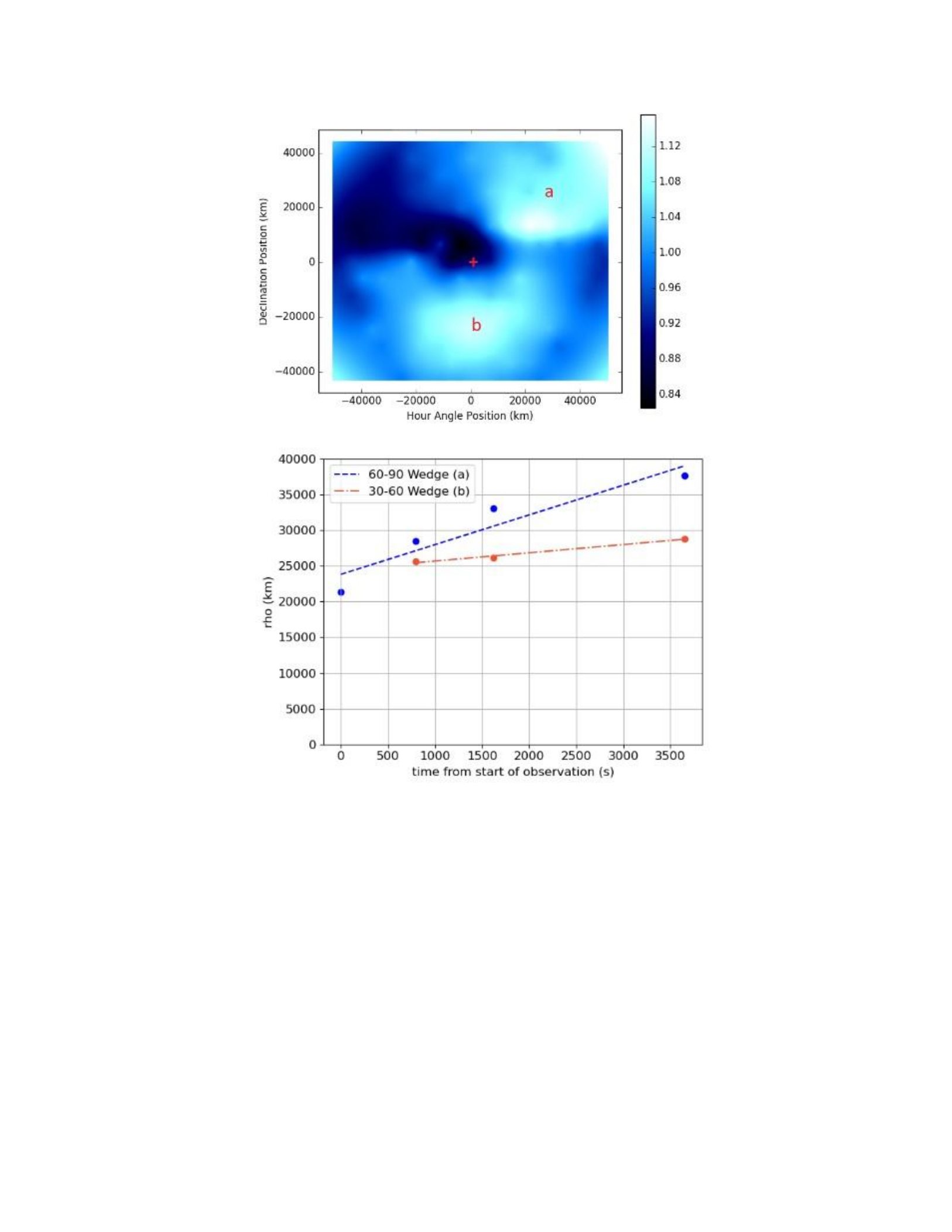
59
Figure 3.2
Outflow feature angular positions
Angular positions of detected features over the timespan of the observations of
Comet Garradd. The above figure depicts an example
𝐶𝑁
radial division map, and
the bottom figure shows the position vs time relation for
𝐶𝑁
over all observations.
The color bar scale on the upper map represents the column density of
𝐶𝑁
. The blue
line of the bottom figure represents feature (a), while the orange line represents
feature (b)

60
3.3 Comparing spatial concentrations
While a qualitative method of visually comparing the model results with enhancement plots
was established, a more quantitative approach was desired as well. A method outlined by
Vaughan [39] for analysis of comet data from the same IFU spectrometer was utilized, where the
enhancement plots were divided into a circle with symmetrical 60° wedges, centered on the
optocenter fiber. The fibers that were located in these position angle wedges were used to
calculate the concentration
ratio Ω,
! !−1
𝐴𝑧𝑖𝐷𝑖𝑣
𝑅𝑎𝑑𝐷𝑖𝑣
1 1
Ω= + + (3.2)
𝜎
2
𝜎
2
𝜎
2
𝜎
2
𝐴𝑧𝑖𝐷𝑖𝑣
𝑅𝑎𝑑𝐷𝑖𝑣
𝐴𝑧𝑖𝐷𝑖𝑣
𝑅𝑎𝑑𝐷𝑖𝑣
where AziDiv and RadDiv correspond to the weighted averages of the azimuthal division values
and the radial division values, respectively, for each fiber. A larger number of fibers within each
wedge allows for more accurate values of Ω, which is why 60° wedges are used, as opposed to
the 30° wedges used in the outflow velocity determinations. If a fiber resides exactly on a line
dividing the wedges, the concentration values are determined from the weighted average of two
symmetric fibers along either boundary of the wedge.
!−1
∑︁
𝐴𝑧𝑖𝐷𝑖𝑣
1
𝐴𝑧𝑖𝐷𝑖𝑣
2
𝑅𝑎𝑑𝐷𝑖𝑣
1
𝑅𝑎𝑑𝐷𝑖𝑣
2
Ω= +
(3.3)
2 2 2 2 2
𝜎
𝜎
𝜎
𝜎
𝜎
𝐴𝑧𝑖𝐷𝑖𝑣
,1
𝐴𝑧𝑖𝐷𝑖𝑣
,2
𝑅𝑎𝑑𝐷𝑖𝑣
,1
𝑅𝑎𝑑𝐷𝑖𝑣
,2

61
where the summation term is
1 1 1
+ +
𝜎
2
𝜎
2
𝜎
2
𝐴𝑧𝑖𝐷𝑖𝑣
,1
𝐴𝑧𝑖𝐷𝑖𝑣
,2
𝑅𝑎𝑑𝐷𝑖𝑣
,1
𝑅𝑎𝑑𝐷𝑖𝑣
,2
The average Ω values are then calculated for each wedge for each moment of observation.
The Ω
𝑎𝑣𝑔
values for each comet and observation are shown in Appendix A. This method is known
as
Welch’s Analysis of Variance (ANOVA).
Since the model does not simulate discrete fibers, the concentration is simply determined by
dividing the final output into 60° wedges and calculating the ratio of the number of particles in
each wedge with the overall total particles produced for the simulated comet nucleus. With
concentration values organized in this way, we now have an additional method of comparing the
model results with our observed enhancement plots after they have been initially constrained by
eye.

62
CHAPTER IV
RESULTS
The rotation of the comet is accounted for by setting a principal axis of rotation and including
a parameter for a change in angular position for set time-step intervals. Each time-step of the
model corresponds to the observations from the IFU spectrograph. For each time-step, the
particles within the active regions are checked against the release probability function. If they
pass the check, they are emitted radially outwards from the nucleus. If they do not pass, the
particle remains on the nucleus as it rotates in each interval. This process is repeated for every
time-step, with the emitted particles continuing their outward motion based on the outflow
velocity values. Non-released particles have a chance to pass the release probability check with
every step.
The outputs from the three-dimensional model are manually analyzed in a two-dimensional
grid to compare with the observable features as seen on the plane of the sky in the 2-D contour
plots. The rotational period of our coma model was adjusted until we were able to approximate
an acceptable fit to our observations obtained with the IFU. A sample output of the model is
shown in
Figure 4.1 on the following page.
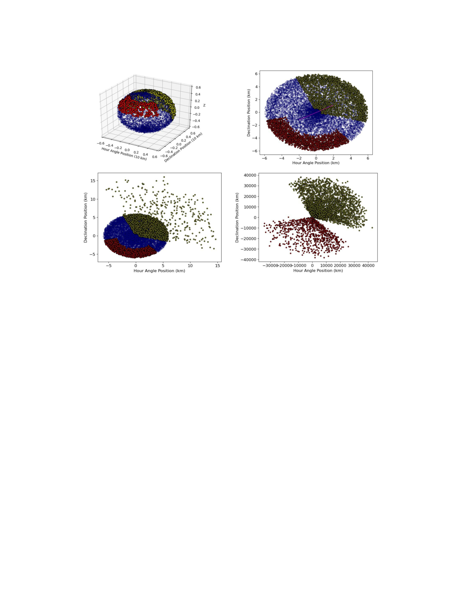
63
Figure 4.1
Sample nucleus of model
The top left image shows an initial setup in three dimensions, while the figure on the
top right depicts the respective setup in two dimensions, with the z-axis increasing
out of the page as the nucleus would be seen on the plane of the sky. The colored
circles represent the modeled particles. Inactive particles are blue, and the separate
active regions are shown in red and yellow. The two-dimensional plots are primarily
used to compare our results with the IFU observations. The bottom figures
represents subsequent timesteps.
4.1 10P/Tempel 2
Comet 10P/Tempel 2 is a Jupiter-family comet that was observed with the IFU spectrograph.
Tempel 2 has been a subject of much analysis from outside sources [23], making it a useful body
for comparison. The effective radius of the nucleus was determined to be 5.98 ± 0.04 km [24],
which is very large for a JFC. The rotation period was determined to be 8.950 ± 0.002 hours by

64
Knight et al. [21] at the time of its 2010/2011 perihelion approach. Furthermore, the period was
also determined to have increased slightly between perihelion passages in 1988 and 1999,
possibly due to systematic torque [23].
From our radial division maps for the carbon-bearing radicals of Tempel 2, we were able to
determine one large primary feature in the coma, as shown in Figure 4.2 on page 27. This area of
high column density was present in our observations from 2010 July 15 and September 13,
suggesting they are from the same active source. The angular position of the feature changes
very little between observations taken on each date, suggesting that the active region from which
it originates is located near a rotational pole. A similar feature was observed from the
𝑁𝐻
2 radial
division maps, though it is smaller in size.
Our Monte Carlo model was constrained to see if similar conditions could be observed from
the output. Thirty cases were produced from a parameter range, and the best fit was visually
chosen from among them. The parameters used for the final Tempel 2 simulations are shown in
Table 4.1 on page 26. The resulting images are shown in Figure 4.3 on page 28
Tempel 2 illustrates one of the main limitations with our model: working with a small number
of observations. Tempel 2 was observed with the IFU spectrograph for only two nights, both with
a small temporal range. Observation times are detailed in Table 4.2 on page 26. As comet
rotational periods tend to be at least several hours long, the available observations only offer a
glimpse at the spatial behavior for comparison with the simulation results. Furthermore, coma
plots from each enhancement date show only a single feature for all radical species, limiting our
ability to constrain our simulated plots by our usual visual standards.
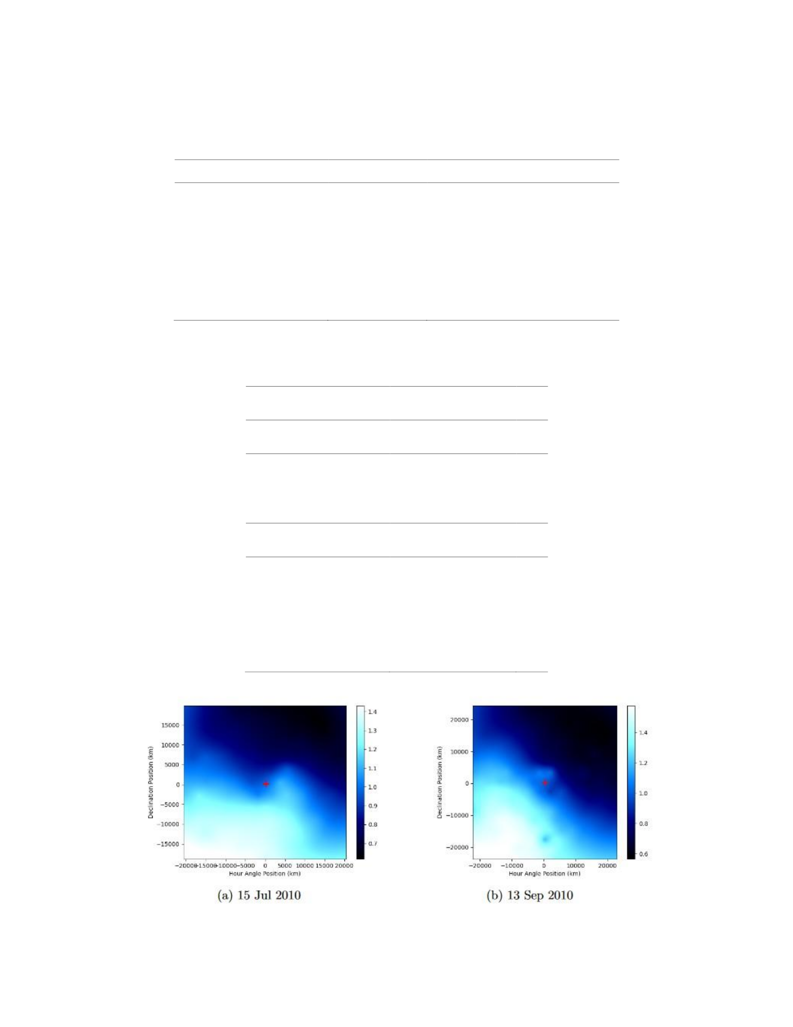
65
Table 4.1
Tempel 2 Model Parameters
Parameter Name
Value
Source
Radius
6 km
Lamy & Toth et al. 2009 [24]
Outflow velocity
0.6 km/s
Knight et al. 2012 [23]
Solar Vector Angle
109°
NASA Horizons
Rotation period
8 ± 0.5 hours
Custom parameter output
Active Area Fraction
34.3 ± .01 %
Random parameter output
Number of test cases
30
Result
Table 4.2
Observation times for Tempel 2
Observation Label
Start Time (UTC)
July 15 2010
278
08:39
300
279
08:48
600
280
09:03
900
September 13 2010
400
09:08
600
401
09:22
900
402
09:39
900
407
11:08
900
408
11:25
600

66
Figure 4.2
Radial division maps for
𝐶𝑁
in Tempel 2
ThelargeactivefeaturecanbeseeninthelowerleftinboththeJuly(left)andSeptember
(right) observations, suggesting little dynamic activity in this period of the comet’s orbit.

67
Figure 4.3
Plots for Comet Tempel 2 from the Monte Carlo model
The first image shows one of the earliest time-steps for the simulation, while the last
shows the resultant plot after a simulated passage of a little over 8 hours. The purple
line running through the nucleus in the left plot denotes the simulated primary
rotation axis, which is partially perpendicular to the plane of the figure.
4.2 C/2009 P1 (Garradd)
Our observations of comet Garradd showed a continuous feature present in the upper right
quadrant of the division maps for the carbon-bearing radicals, as seen in Figure 4.4 on page 32.
This suggests a relatively simple rotational mode for the comet, with the feature possibly
originating near the pole of the primary rotational axis. As such, we first tested our simulation by
inputting parameters from Garradd that were observed and also supported by other sources.
These are given in Table 4.3 on page 31. Due to the appearance of two features, a wider test case
of about seventy runs was required for a best-match simulation. Observation times are shown in
Table 4.4 on page 31, with each observation having a 600 second duration.
Figure 4.5 on page 34 shows comparisons between sample radial division plots and model
simulation results that most visually resemble them. The simulated total active area fraction was
generated as 49.5%, which would support our estimate that Garradd is a highly active comet. The

68
water production rates measured by Boissier et al. [6] suggests an active area fraction of at least
50%. One notable distinction from the model output is the lower concenctration of particles in
the feature in the bottom of the map for Figure 4.5b. This can be due to limitations with the
model, or it could indicate a more complex rotational mode for Garradd than was initially
assumed, as the feature is not present for the entire night of observations. It could also be due
to the fact that the simulated nucleus is stationary, with the only motion being due to rotation.
In reality, the comet is travelling through space as it orbits the Sun, so if an active jet were to
rotate away from view, we wouldn’t still be seeing all the residual outflow. All the carbon-bearing
radicals appear to have similar morphologies over our observation period, suggesting they
originate from the same source regions on the surface of the nucleus.
𝐶𝑁
is typically chosen for
primary visual comparison, as it has a better contrast in the coma compared to the other radicals
due to the strength of the violet band [23].
The concentration ratio of the active particles in the simulation shown in Figure 4.5 on page
34 match the Welch’s ANOVA wedge concentration spread, with the 0°, 240°, and 300° wedges
having the most activity across both. There is a difference in that the 0°-60° wedge in the model
has a slightly higher concentration than the 240°-300° wedge (27.5% and 28%, respectively) while
the relationship is reversed in the ANOVA concentrations found for
𝐶𝑁
, as shown in Appendix A.

69
Table 4.3
Comet Garradd Model Parameters
Parameter Name
Value
Source
Radius
5.6 km
Boissier et al. 2013 [6]
Outflow velocity
1-25 m/s
Mazzotta et al. 2016 [29]
Solar Vector Angle
139°
NASA Horizons
Rotation period
8 hours
Custom parameter
Active Area Fraction
49.5%
Random parameter
Primary Rotation Axis
𝜋
/6
Random Parameter
Number of test cases
75
Result
Table 4.4
Observation times for 2009/P1 Garradd
Observation Label
Start Time (UTC)
August 21 2011
944
02:45
946
03:12
948
03:46
950
04:16
952
04:47
958
06:18
960
06:50
962
07:21
964
07:53
966
08:26
968
08:59
August 22 2011
1028
02:53
1029
03:08
1034
04:34
1035
04:46
1039
05:52
1042
06:35
1046
07:40
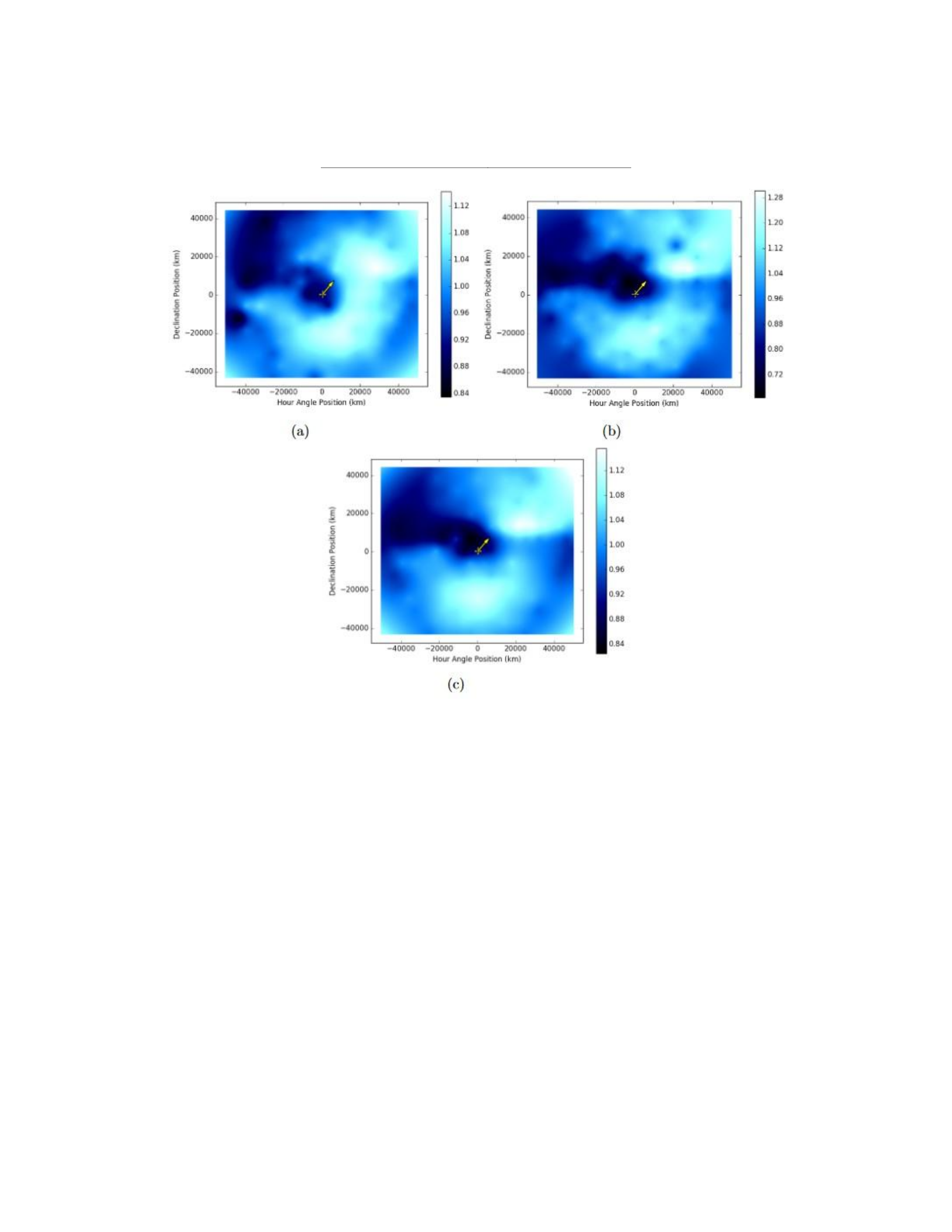
70
1051
09:01
1054
09:39
Figure 4.4
Radial division maps for Comet Garradd
Observations taken on the night of 2011 August 21 at 06:18 local time. The color bars
represent the column density of the detected radical. The white feature that can be
seen in the upper right is present for most of the night’s observations. This suggests
an active region rich in carbon-based molecules. The small yellow crosses represent
the locations of the optocenter, and the arrows represent the direction of the solar
vector. The solar vectors are pointing mostly out of the screen. The maps depict
𝐶
2,
𝐶
3, and
𝐶𝑁
, respectively.
While the spatial distributions of the carbon-bearing radicals are very similar to each other,

71
𝑁𝐻
2 exhibits a very different outgassing behavior for Garradd. Two coma features can be seen
opposite to each other on the top and bottom parts of the enhancement plots, similar in
appearance to an hourglass. This indicates that the features originate from two separate sources,
with the bottom source being different than the active region responsible for the carbon-bearing
radicals. These plots and their respective model simulation comparisons are shown in Figure 4.6
on page 35. The active particle spread most matches the ANOVA concentrations of the August 22
observations, with the wedges in the 60°-120° and 240°-360° regions showing the highest density
(14.4%, 24.2%, and 25.7%, respectively).
Both the
𝑁𝐻
2 and
𝐶𝑁
simulations had the same generating parameters, showing how they
could have separate morphology and possible source regions and yet arise from the same
rotational state. The model simulated a timespan of 292 hours with timesteps of 300 seconds.
Our best comparison plots were produced from an initial parameter for rotation period of 8 ± 0.5
hours. This is lower than values obtained from other authors. Farnham et al. [12] determined a
value of
10.4 ± 0.05 hours from lightcurve measurements, while Ivanova et al. [18] determined a period
of 11.1 ± 0.8 hours using a cross-correlation method of tracking a morphological feature over
time, similar to our own. Due to the wider number of available usable observations for Comet
Garradd, an additional method for checking the period was done by determining our own
lightcurve from the enhanced plots. The phase determined from this method also corresponded
with a period of 8±0.75 hours, which agrees with our model result. This suggests that this value
is at least consistent with our own observations. The lightcurve is shown in Figure 4.7 on page
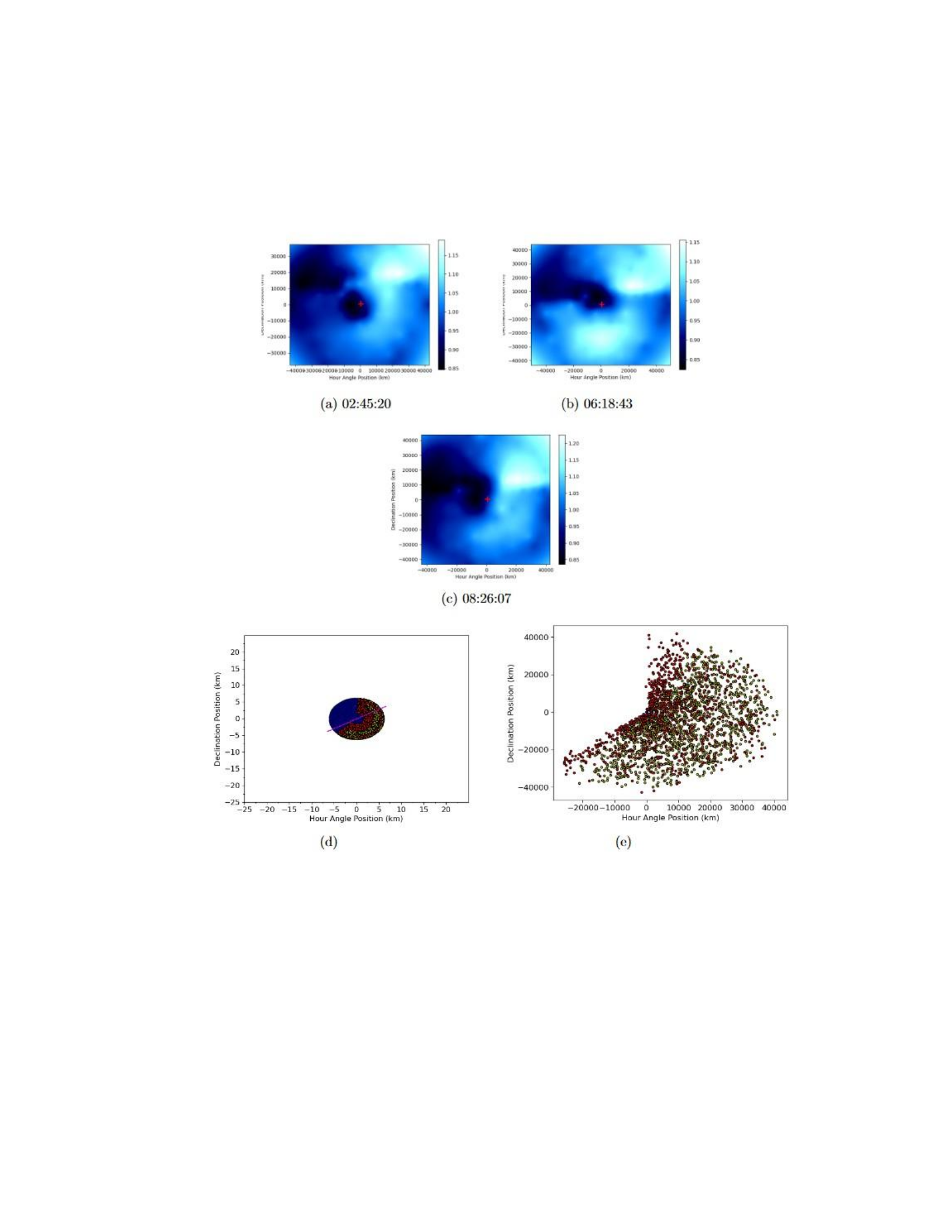
72
36. The discrepancy of our results from the others determined may be due to our different
observation methodology.
Figure 4.5
Garradd model CN comparison
Comparisons between radial division maps for
𝐶𝑁
in Comet Garradd and simulated
maps from the Monte Carlo model. The top three images show results over the night
of 2011 August 21 and their respective observation timestamps. The bottom row
shows maps randomly generated by the model that appear visually closest to the
enhancement plots, with the left being the initial generated nucleus and the right
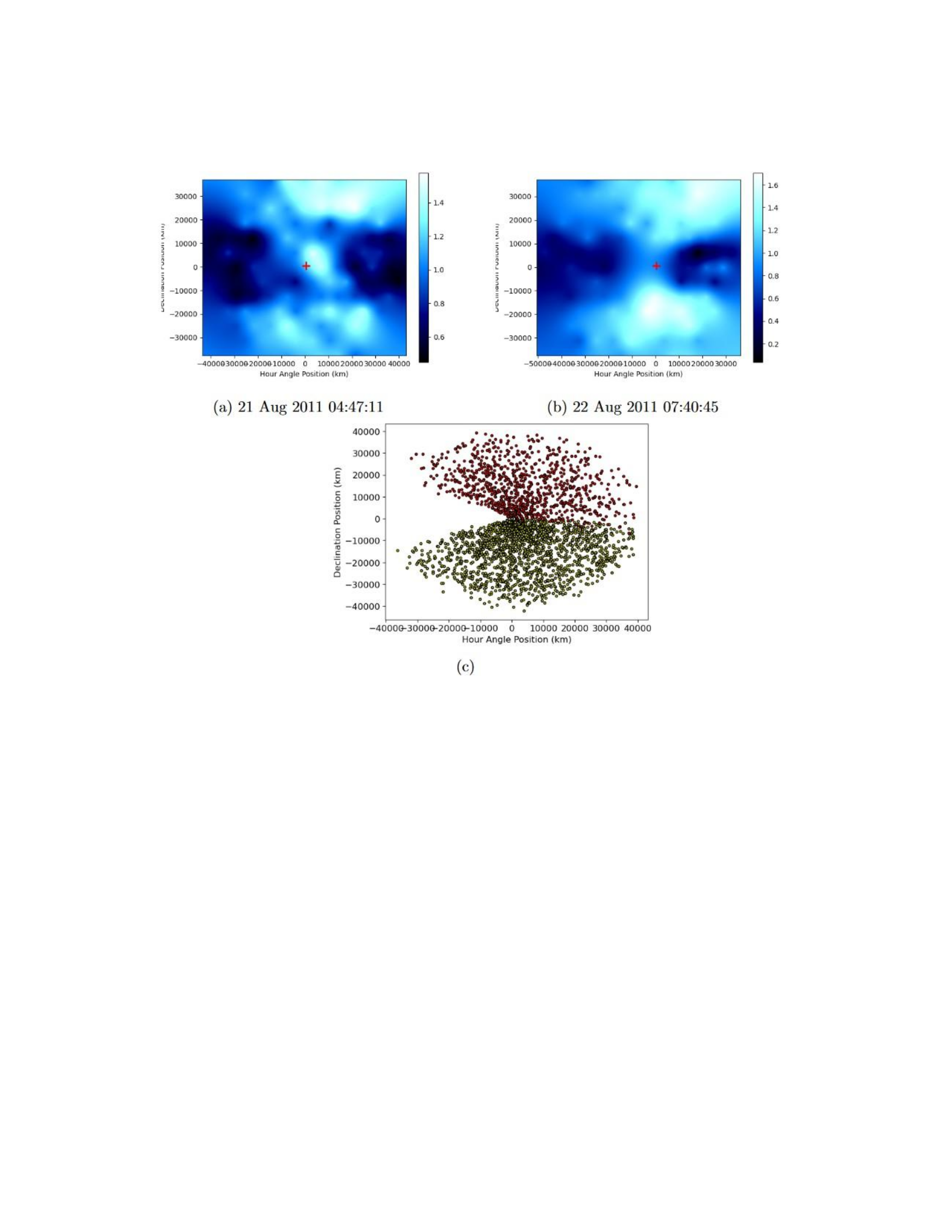
73
being the result after several timesteps. The purple line running through the nucleus
in the left plot denotes the simulated primary rotation axis.
Figure 4.6
Garradd model NH2 comparison
Comparisons between radial division maps for
𝑁𝐻
2 in Comet Garradd and simulated
maps from the Monte Carlo model. The top images show a sample observation over
two different nights. The bottom row shows a map randomly generated by the model
that appear visually closest to the enhancement plots.

74
Figure 4.7
Garradd enhancement plot lightcurve
Lightcurve determined from our enhancement plots for our observations taken over
two nights. The blue dot represent observations taken on August 21, red dots
represent August 22. A phase (gray sine curve) was determined from similar
morphological features found in the enhancements of all radicals across both nights.
4.3 168P/Hergenrother
Comet Hergenrother presented unique challenges compared to our other comets. It is
another Jupiter Family Comet, whereas Garradd is a long-period comet, and thus likely has
different physical properties in terms of nucleus size and active area fraction, and a lot less is
known about Hergenrother as opposed to the other comets in this study. In terms of radicals,
Hergenrother was found to be extremely chemically depleted [33], allowing only viable
observations for
𝐶𝑁
. Only one bright feature can be seen in the
𝐶𝑁
maps, shown in Figure 4.8 on
page 41, so only one active area was set in the model. Fifty runs were required for Hergenrother

75
as well. The closest visual simulations are achieved by setting a rotation period parameter of 6.5
hours, and are shown in
Figure 4.9 on page 42. The other model parameters are shown in Table 4.5 on the following page.

76
Table 4.5 Comet Hergenrother Model
Parameters
Parameter Name
Value
Source
Radius
0.7 km
Custom
parameter
Outflow velocity
1-15 m/s
Custom
parameter
Solar Vector Angle
159°
NASA Horizons
Rotation period
6.5 ± 0.5 hours
Custom
parameter
Active Area Fraction
19.4 ± .01%
Random
parameter
Number of test cases
50
Result
Table 4.6 Observation times for
168P/Hergenrother
Observation Label
Start Time (UTC)
October 06 2012
1200
05:09
1201
05:35
1202
06:00
1203
06:55
1204
07:18
October 08
1307
02:57
1308
03:20
1309
03:42
1310
04:06
1314
05:39
1315
06:02
1320
08:01
October 09
1372
02:20
1373
02:44
1377
04:18

77
1378
04:42
1381
05:53
1384
07:01
1389
08:55
December 19 2012
1423
01:14
1424
01:48
December 20
1514
06:43
December 21
1577
01:15
1578
01:47
The active area fraction for the surface of the nucleus was 19.4 ± 0.01% for this best-match
simulation. This is much lower than the best-match runs for Garradd, which coincides with our
observation that Hergenrother is chemically depleted and less active compared to most comets
[33]. It remains to be seen if the depletion of Hergenrother, or its recent lack of detection near
its last expected perihelion [41], are related to the aforementioned fragmentation event. The
model constrainstherotationperiodforouranalysisof168Pto6.5±0.5hours.
Therearenomeasurements of Hergenrother’s rotation period from outside sources with which to
compare our result.
Due to the aforementioned chemical depletion, Welch’s ANOVA wedge comparisons were
done with our measurements of
𝐶𝑁
. The simulation output yield concentrations in the 0°-60°,
60°-120°, and 300°-360° wedges of 36.1%, 32%, and 28.5%, respectively. The actual ANOVA
calculations show higher wedge concentrations primarily in the 0°-60°, 240°-300°, and 300°-360°
regions, differing slightly from our model. This indicates that our model results may not align to
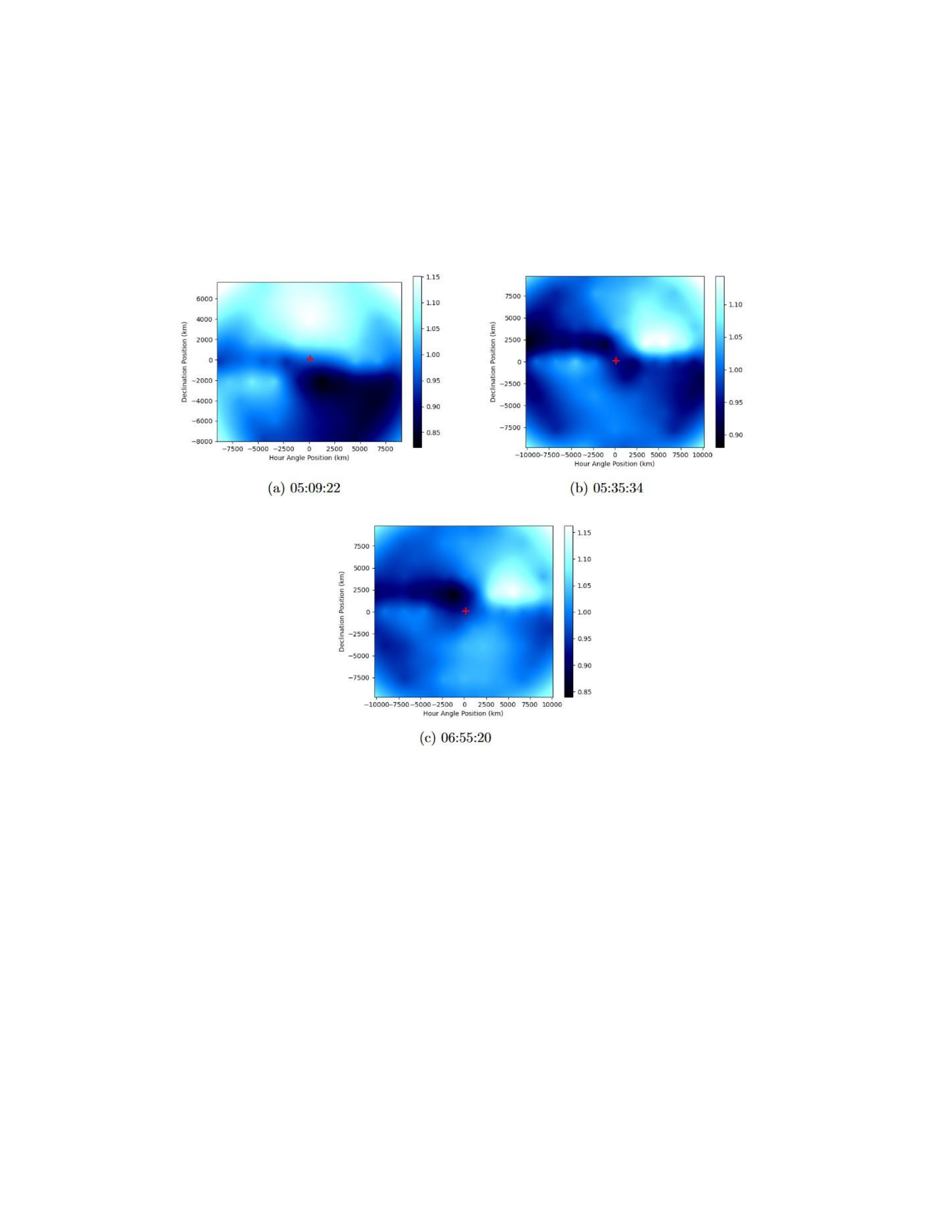
78
our observations with high precision. It is difficult to further constrain, as almost half of our
Hergenrother observations were dominated by a low signal-to-noise ratio, which can affect the
amount of usable fibers in the ANOVA calculations.
Figure 4.8
Hergenrother maps
𝐶𝑁
radial division maps for Comet Hergenrother on the night of 2012 October 6. Due
to the small interval of time coverage of the observations shown, the singular bright
feature in the upper right of each map moves very little between images.
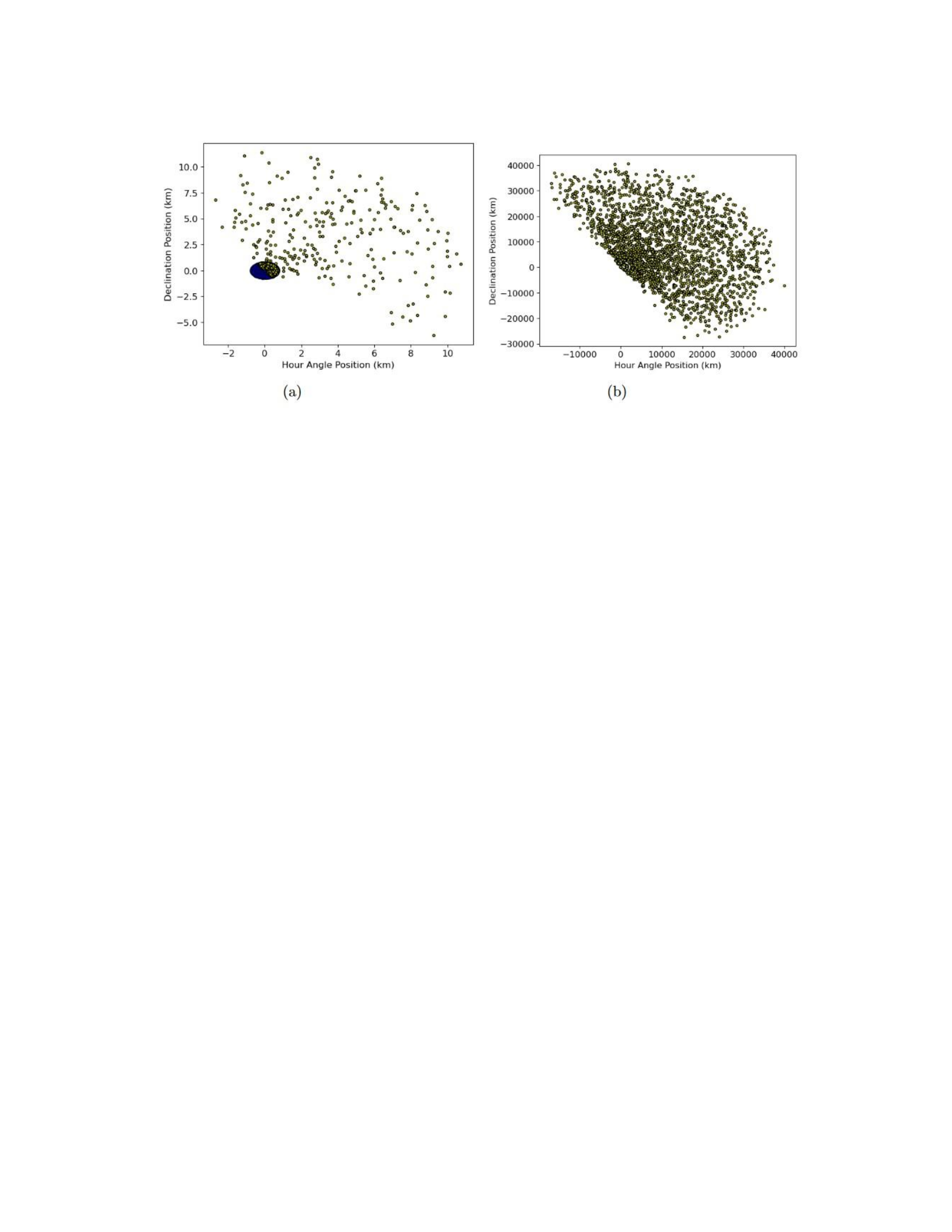
79
Figure 4.9
Hergenrother model CN comparison
Plots for Comet Hergenrother from the Monte Carlo model. The first image shows
one of the earliest time-steps for the simulation, while the last shows the resultant
plot after a simulated passage of about 290 hours. The purple line running through
the nucleus in the left plot denotes the simulated primary rotation axis.
CHAPTER V
CONCLUSION AND FUTURE WORK
The rotational period parameters that were set for the best-matching model results for each
comet were very close to the period constrained by either other sources or by visually tracking
the periods over multiple observations. The model also simulates possible active area fractions
for the comets and their approximate locations on the surface. These parameters are not well
constrained by observation alone, so these values can be of interest to other parties. The values
determined for active area fractions (34%, 50%, and 19% for Tempel 2, Garradd, and
Hergenrother respectively) suggests that long period comets like Garradd have higher active area

80
fractions than JFC’s such as Tempel 2 and Hergenrother, as they have experienced more
outgassing and perihelion passages.
Other methods of visually inferring rotational states of comets involves working with data
taken via multiple observations over a long timespan, typically months apart. The data for our
comets were only collected over a couple concurrent nights by the George and Cynthia Mitchell
IFU Spectrograph, limiting the long-term comparisons that could be done with our model. As
such our model results are only effective as comparisons with specific “snapshots" of the comets’
behavior. Further constraints could be placed with further observations, especially comparing
preand post-perihelion activity.
Future efforts will be spent on improving the model. Dust and gas are two very different
components of comet composition and exhibit different outflow behavior, especially beyond the
first few kilometers after release from the nucleus. Our reduced division maps from the IFU
spectrograph are based primarily on the gas located in the outer coma, and we must be cautious
in establishing a link to the dust outflow from the nucleus generated by the Monte Carlo model.
While both may come from similar jet sources, gasinteractions typically require parent-daughter
molecule interactions. A possible method of improvement would be to implement techniques
from a similar Monte Carlo model by Lederer et al. [25], in which trajectories of parent molecules
are tracked, and possible daughter decays are simulated by a exponential decay function. The
daughter molecules are ejected isotropically from the parent, and both are subsequently tracked
vectorially in the coma [25]. Additionally, the current version of the Monte Carlo model only
accounts for simple rotation around a primary axis. A more realistic model can be attempted by

81
accounting for more complex rotational states, such as precession and nutation, that have been
observed for other comets, such as Hartley 2 [4]. The comet’s translational motion as it moves
along its orbital path around the Sun could also be considered to eliminate residual outflow
between timesteps. Further checks must also be made to ensure uniqueness of our model
simulations, as multiple three-dimensional configurations of active area locations could
theoretically produce visually similar two-dimensional plots. The parameters of the model can be
adjusted accordingly as more information on our comets is corroborated and published by
outside sources.
CHAPTER I
INTRODUCTION
Scientists across multiple fields, not just physics and astronomy, have an interest in comets
and their connection to the formation of the solar system. Many questions concerning the
chemical and biological evolution of life on Earth involve the early conditions of the planet.
Accretion of material in the outer distances of the solar system led to the formation of comets.
Initially postulated as “dirty snowballs” [40], recent observations of the composition of comets
led astronomers to view them more as “icy dirtballs”, consisting mainly of ice, rock, and organic
compounds that coalesced
togetherintolowdensitystructuresduringtheearlyageofthesolarsystem, over4.5billionyearsago
[3]. Thiscompositionappearstoholdtrueevenforobservedinsterstellarcomets, suchas2I/Borisov

82
[8], which was observed passing through our solar system in 2019. Comets are usually grouped
by their orbital characteristics, with the longer-period comets originating from distant small-body
populations such as the Kuiper Belt, the scattered disk, and the Oort Cloud. The existence of these
populations support a model of the evolution of the solar system known as the Nice model,
where the gas giants were in more cicular, closely spaced orbits at the edge of the inner disk.
Small icy bodies were scattered by the gas giants inwards, which caused Saturn, Uranus, and
Neptune to migrate outwards due to conservation of angular momentum [38]. Further
interactions with Jupiter caused the icy bodies to enter highly elliptical orbits, while Jupiter
migrated slighty inwards towards its current postion. An alternative model known as the grand
tack hypothesis proposes that Jupiter instead initially migrated inwards from a distance of 30 AU
and then outwards after capturing Saturn in a mean-motion resonance [26]. This hypothesis has
developed more recent support from studies of comets C/2014 S3 (PANSTARRS) and
67P/Churyamov-Gerasimenko, where the low detection of collisional elements in these outer
bodies corresponds with the early migration of Jupiter and Saturn posited in the grand tack [37].
Comets tend to be less dynamically active and exhibit less change in volatile composition
compared to other major bodies in the solar system. Thus, they provide insight into the physical
and chemical properties of the early conditions of the solar system. Insitu measurements of
comets, such as the Stardust mission, have detected organic molecules, including the amino acid
glycine [9]. Such evidence supports the hypothesis that comets were key to delivering the
precursors to life to early Earth. However, recent studies into comets, including the Rosetta
mission, have measured the Deuterium-to-Hydrogen (D/H) ratio, which was determined to be at

83
least three times greater than the ratio for the Vienna Standard Mean Ocean Water (VSMOW) on
Earth, (1.5576±0.0001)×10−4 [27]. This suggests the opposite to the long-held idea that comets
were also the means through which water came to our planet. Cometary science is still rapidly
changing and can still provide much in the way of constraints of the formation of Earth and the
solar system.
The majority of comets fall within two categories: short-period and long-period comets, based
on whether their orbital revolution periods are less than, or greater than, 200 years. Most short
period comets, known as Jupiter-family comets (JFCs), are theorized to have originated from
beyond Neptune, in the scattered disk of the Kuiper Belt region. They tend to orbit in the same
ecliptic plane as the planets and have periods of less than 200 years. The exception to these are
the Halley-family comets. While they also have a short orbital period, they are highly inclined to
the ecliptic, suggesting a different region of origin: the distant Oort Cloud. Proposed by Jan Oort
in 1950, the Oort Cloud is a theoretical, spherical region of space dominated by icy planetesimals
that were theorized to have formed during the same time period as the planets [32] [10]. Long-
period comets by contrast are highly eccentric, leading to orbital periods that range from
hundreds to thousands of years. These long-period comets are also thought to have originated
from the Oort Cloud. As many have hyperbolic trajectories, long-period comets will only have a
single solar apparition before they escape the solar system.
Due to their possible connection to the formation of the solar system, comets are the subject
of numerous chemical surveys [15]. Narrow-band photometry [1] and spectroscopic surveys [7]

84
have shown that the majority of comets are similar in chemical composition, with the exception
that a significant fraction of JFCs are depleted in carbon-chain molecules. Observations of the
dust-to-gas ratio and the abundances of carbon-based radical species (
𝐶𝑁
,
𝐶
3,
𝐶
2, etc.) show little
correlation based on composition or dynamical family. The subtle variances exhibited in the
comets based on their classes suggest differences in dynamical evolution rather than different
conditions of formation [7].
Due to the nature of comets, many properties have to be inferred from the types of radiation
we can detect remotely, as in situ observations are a rare opportunity. One such property is the
rotational period of the comet, which has most commonly been determined from the measured
lightcurve. If a celestial target such as a comet is observed over a long enough period, it is possible
to graph the flux or intensity of the measured light over time. If periodicity is seen in the
lightcurve, then it is possible to determine a spin period of the nucleus. Further constraints could
be made if multiple lightcurves are made over a range of heliocentric distances, as was made
with 1P/Halley [14]. Active areas are determined from spherical nucleus approximations, even
though they tend to be elliptical in nature. Constraints are made based on the size and flux of
emission sources, and are determined as fractions of the surface area of the nucleus [20].
1.1 Target comets
The comets examined in this research were C/2009 P1 (Garradd), Comet 168P/Hergenrother,
and Comet 10P/Tempel 2. Garradd was an active, dynamically young, long-period comet at the
time of observation, likely making its first trip through the solar system. The comet is in a highly
eccentric orbit of e = 1.001, and has an inclination of 106.18 degrees. Comet Hergenrother is a

85
Jupiter-family comet with an orbital period of about 6.90 years. It has an orbital eccentricity e =
0.610, and an inclination of 21.93 degrees. Tempel 2 is also a JFC, with e = 0.5363, an inclination
of 12.02 degrees, and an orbital period of about 5.5 years.
Comet Garradd was very active during its pre-perihelion transit, with one of the highest dust-
to-gas ratios and water production rates observed in a comet [5]. The
𝐶𝑂
2/
𝐻
2
𝑂
and
𝐶𝑂
/
𝐻
2
𝑂
ratios were measured from September-October 2011, and in January-March 2012, and were
found to be less abundant post-perihelion [5]. Since the ices in comets are primarily composed
of these volatiles, we can determine how the activity is driven during the comet’s passage. An
asymmetry between the two ratios from pre- to post-perihelion also suggests either a large-scale
chemical heterogeneity in the nucleus [30], or that the rotational state led to an effect where one
hemisphere was exposed to more activity from solar exposure than the other [13]. It also had a
high active surface area to nucleus area ratio.
Comet Hergenrother was a recently discovered comet, of which few publications exist. It
underwent an outburst in 2012, which may have resulted in a fragmentation event a few weeks
afterward and has been reported as overdue for its 2019 apparition after it was not detected
near its expected perihelion passage. [41]. Pierce and Cochran [33] performed spectroscopic
analysis of Hergenrother and found it to be the most depleted comet reported in
𝐶
2,
𝐶
3, and
𝑁𝐻
2.
Observations of such events can provide unique insight into the chemical and physical properties
of comets during a period of high activity. Fragments of Comet 73P/Schwassmann-Wachmann 3
were observed to have similar chemical properties but physical heterogeneities [16]. The
fragmentation event itself can also affect the dust production, such as with C/1994 S4 LINEAR [2],

86
or the orbital parameters, as with the Kreutz sungrazers, a family of comets believed to have
originated from a common progenitor comet that fragmented into two parts during a past
perihelion approach within 3.45 solar radii [19]. These super-fragments were then believed to
have undergone their own fragmentation events upon subsequent perihelion passages [36].
In contrast, 10P/Tempel 2 has been extensively studied since its discovery in 1873. Its short
orbital period, allowing for multiple observations over dozens of apparitions, as well as it once
being a possible target for a flyby mission, has made it the object of numerous ground-based
studies. Its next close approach to Earth is due to occur in August 2026 with a nominal geocentric
distance of 0.41 AU. It has been observed to have low outgassing activity and brightness pre-
perihelion, and has a typical dust-to-gas ratio of other comets with a similar perihelion distance
[23].
CHAPTER II
OBSERVATIONS
Observations of comets primarily focus on two components: the nucleus and the coma. The
nucleus corresponds to the solid part of the comet. Nuclei are typically comprised of dust and
ice, and tend to have a size range on the order of a few to tens of kilometers. As the nucleus is
exposed to heat from the Sun, the ices trapped on or below the surface can sublimate. The
resultant atmosphere of gas surrounding the nucleus is known as the coma. As the comet
approaches the Sun, the visible coma can increase in size to an order of tens of thousands of
kilometers in diameter, as ice grains can continue to sublimate as they’re dragged outwards by

87
the gas. Due to the low albedo and smaller size of the nucleus compared to the coma, direct
observations of the nucleus are usually restricted to in situ measurements. For comets Garradd
and Hergenrother, the measurements for this study were taken of their respective comae from
ground-based telescopic observations. The observations for Comet Garradd were obtained pre-
perihelion, while the Hergenrother and Tempel 2 observations were obtained post-perihelion.
Specific observation and calibration parameters for Garradd, Hergenrother, and Tempel 2 are
shown in Table 2.1 and Table 2.2 on page 8.
ThecomaobservationswereobtainedwiththeGeorgeandCynthiaMitchellSpectrograph. This
integral-field unit (IFU) spectrograph is a low- to moderate- resolution fiber optic spectrograph
consisting of 246 optical fibers. The optical fibers each have a diameter of 4.1 arcsec and are
arranged in a 1.7 x 1.7 arcmin array, alternating from 14 to 15 bundled fibers per row [17]. A
diffraction grating covered the passband from 3600-5800 Å and provides a spectral resolving
power (
𝜆
/Δ
𝜆
) of 850. The spectrometer was used in conjunction with the 2.7 m Harlan J. Smith
Telescope located at McDonald Observatory in Fort Davis, Texas. In order to maintain the comet’s
position on the array, a tracking star is used with a fiducial that moves opposite to the comet’s
motion. Any star spectra caught crossing through the field of view are removed in analysis [33].
Observations were taken of various radical species with spectral emission bands visible in
the spectrometer’s passband, including
𝐶
2,
𝐶
3,
𝐶𝐻
,
𝐶𝑁
, and
𝑁𝐻
2. Each fiber in the array was
connected to a charge-coupled device (CCD) and yield independent spectra. The raw data were
initially reduced through bias subtraction, flat fielding, and calibration in flux and wavelength.
Since the measured spectra are a mix of the emission bands from the coma superposed on a

88
continuum from the reflection of the solar spectrum off the dust in the coma, analogue stars
were utulized. Each night the flux and color of a solar analog star is matched with the observed
comet’s spectrum, and the solar spectrum is subsequently removed.
Table 2.1
Comet Observation Parameters
Comet
Obs. Date
r
𝐻
1
Δ2
Phase Angle3
Pre/Post
(UT)
(AU)
(AU)
(Degrees)
Perihelion
10P/Tempel 2
2010 Jul 15
1.43
0.72
42.2°
Post
2010 Sep 13
1.60
0.67
21.8°
Post
C/2009 P1 (Garradd)
2011 Aug 20
2.28
1.40
16.1°
Pre
2011 Aug 21
2.27
1.39
16.4°
Pre
2011 Aug 22
2.26
1.39
16.9°
Pre
168P/Hergenrother
2012 Oct 6
1.42
0.44
14.8°
Post
2012 Oct 8
1.42
0.44
16.1°
Post
2012 Oct 9
1.42
0.44
16.7°
Post
2012 Dec 19
1.66
0.99
32.7°
Post
2012 Dec 20
1.66
0.99
32.7°
Post
2012 Dec 21
1.67
1.00
32.7°
Post
Table 2.2
Comet Calibration Targets
Comet
Obs. Date (UT)
Flux Standard
Solar Analogue
10P/Tempel 2
2010 Jul 15
Feige 98
None
2010 Sep 13
BD+25 3941
HD 191854
C/2009 P1 (Garradd)
2011 Aug 20
BD+25 3941
39 Tau
2011 Aug 21
Feige 15
HD 6204
2011 Aug 22
BD+28 4211
HIP 109931

89
168P/Hergenrother
2012 Oct 6
Feige 15
HD 19518
2012 Oct 8
BD+28 4211
HIP 109931
2012 Oct 9
BD+28 4211
16 Cyg B
2012 Dec 19
Feige 15
Hyades 64
2012 Dec 20
Feige 34, Feige 56
35 Leo
2012 Dec 21
Feige 15, Feige 25
Hyades 64, HD19518
The reduced data were separated into columns representing the fiber number, the base-10
logarithm of the projected distance from the comet nucleus (
𝑙𝑜𝑔
(
𝜌
)), the logarithm of the column
density of the respective radical (
𝑙𝑜𝑔
(
𝑁
)), and the
𝑥
and
𝑦
coordinates of the coma measurement
from the comet nucleus. For the Garradd and Hergenrother data,
𝑥
corresponded to the hour
angle offset in kilometers, and
𝑦
corresponded to the declination position in kilometers. The
radial distance from the comet nucleus,
𝜌
, was determined by the distance formula
√︃
𝜌
=
𝑥
2 +
𝑦
2 (2.1)
The optocenter fiber was determined from each observation from the fiber corresponding to the
lowest value of
𝜌
. This single fiber is designated as the position of the comet nucleus.
Raw contour plots were generated for each observation, with the variables corresponding to
the
𝑥
and
𝑦
values for each observation, and the contour levels corresponding to the
𝑙𝑜𝑔
(
𝑁
) values.
The data were then analyzed based on their arrangement about the optocenter. In order to model
enhanced coma features as a function of projected distance from the nucleus, azimuthal rings
were determined based on the fibers being arranged in concentric, hexagonal rings about the
optocenter.

90
For each pixel in the ring, the projected distance was measured from the optocenter by
√︃
|
𝜌
−
𝜌
0| = (
𝑥
−
𝑥
0)2 + (
𝑦
−
𝑦
0)2 (2.2)
where
𝑥
0 and
𝑦
0 representthehorizontalandverticalpositionoftheoptocenter,and
𝑥
and
𝑦
represent
the horizontal and vertical position of the respective pixel. For each pixel in each azimuthal ring,
the values for |
𝜌
−
𝜌
0| were averaged, yielding an averaged radius value (
𝜌𝑎𝑣𝑔
). The column
densities for each fiber in the ring were also averaged, yielding an azimuthally averaged column
density value
𝑁𝑎𝑣𝑔
. In order to describe the relationship of the column density of each radical
with respect to the projected distance from the nucleus, a relationship
𝑁𝑚𝑜𝑑𝑒𝑙
was determined,
𝑁𝑚𝑜𝑑𝑒𝑙
=
𝐶
|
𝜌
−
𝜌
0|
𝑘
, (2.3)
where
𝐶
and
𝑘
are constants determined from a weighted least-squares fit. The fit parameters
were determined from the linear relation
log(
𝑁𝑚𝑜𝑑𝑒𝑙
) =
𝑘
log(|
𝜌
−
𝜌
0|) + log(
𝐶
) (2.4)
To further examine the heterogeneities of the radicals, azimuthal division coma enhancement
plots were generated, with the contour levels corresponding to the column density
𝑁
of each
fiber divided by the respective
𝑁𝑎𝑣𝑔
of the azimuthal ring. Radial division coma enhancement
plots were generated in a similar manner, with the contour levels corresponding to the ratio of
𝑁
over
𝑁𝑚𝑜𝑑𝑒𝑙
for each fiber in the array.

91
These azimuthal and radial coma enhancements can be used to look for coma features such
as jets or arcs. In addition to comparing coma features for each radical species across different
comets, they can also be used to observe how these features change over time. By focusing on
how the features change in position over several observations, we can attempt to link coma
features with changes in the physical nucleus, and recurring coma morphological features can be
used to constrain possible rotational states of the comets. The most common way to constrain
comet rotation periods is through analyzing a measured lightcurve to look for periodic, repeating
behavior [31]. A technique similar to ours used by Esterle [11] with Comet Halley involves
dynamically modeling simulated dust jets about the long axis mode of the comet nucleus over
time, and comparing them with jets seen in ground-based observations. Comparing
spectroscopic features allows for an additional method of analyzing rotation by use of a Monte
Carlo model [22]. Comparisons between the raw, azimuthal division, and radial division contour
plots are shown in
Figure 2.1 on the next page.
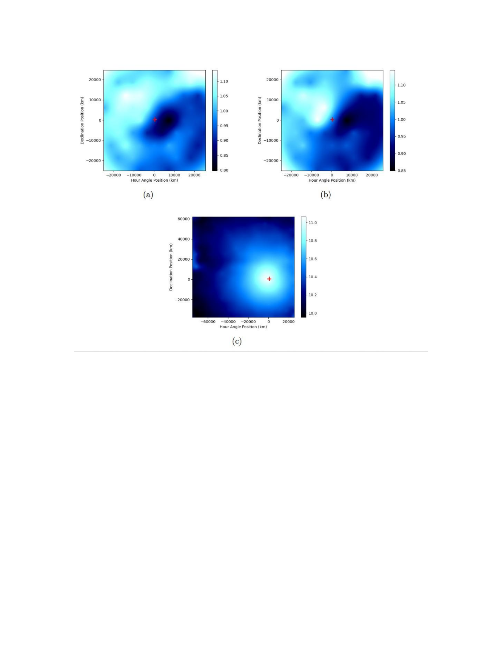
92
Figure 2.1
Sample IFU contour plots
Representations of the radially divided (a) and azimuthally divided (b) contour plots
(top) with their respective raw contour plot (bottom). Plots were of
𝐶
3 measurement
taken from Comet Garradd on 2011 August 22. The raw plot is slightly offset in terms
of the origin, as it is aligned with the optocenter (denoted by the red crosshair) of
the fiber array.
CHAPTER III
METHODS

93
There are no simple methods for analyzing the mechanical behavior of the comet, such as its
rotational motion, from the radical features expressed in the outer coma. We can, however, place
constraints on several parameters by simulation. A Monte Carlo model used by Schleicher and
Woodney [35] outlines a method by which we can use the properties of the detected dust
particles of our radical species and their motion over time to simulate the behavior of the features
found in our coma enhancement plots. Several parameters of the model can be adjusted
manually, and they are usually randomly generated within known boundaries. These include the
positions of the simulated active regions, the number and position of the particles within these
respective active regions, their outflow direction and velocity, and the rotational axis of the
comet, assuming no precession or nutation. Each run of the model will output several images
over a predetermined period of time that corresponds with the timespan of the comet
observations.
The model is used to simulate a variety of cases, with the parameters randomly varied
between each simulation [35]. The visual output of the model is then cross-referenced with the
comet enhancement plots by eye in order to determine a reasonable range of values for the
parameters. They are then adjusted slightly to yield a better overall fit of the simulated particles
with the features shown in the enhancement plots. With these determined physical parameters,
it is possible to constrain a rotational period for the comet.
3.1 The model
The outline for the Monte Carlo model involves generating a simplified, spherically symmetric
modelofthenucleusin3-dimensionalspace. Themodelmustbeinitializedwithseveralparameters

94
including pole orientation, latitudes and longitudes of jet features, outflow velocity of radical
particles, and a set rotational period. A fixed number of particles are generated within the 3D
space, on the order of 104. To determine if features in the outer coma are related to physical
active regions on the surface of the comet’s nucleus, we assume that they are the same quantity.
These particles represent dust grains from active regions of a spherically-symmetric nucleus. The
size of the comet nucleus is based on available literature for the target comet being studied.
Otherwise, if no published values exist, we work within a likely range of values for those comets.
The fraction of the nucleus that is considered active is determined by a pseudo-random number
generator operating within a range of 10 - 60%. The active fraction is constrained to one or more
regions with randomly generated sizes and positions on the nucleus, depending on how many
possible active regions can be determined from the enhancement plots. Particles that are located
within the boundaries of the active regions are sorted into a separate list from the ‘inactive’
particles, and are made visually distinct in the output plots via differing colors. A location for the
solar vector is set based on the comet’s orbital ephemeris at the time of observation. The chance
that a particle is released from the nucleus and emitted into the coma is determined by a
probability function of the cosine of the angle between the respective particle’s position and the
solar vector. If the particle is released from the nucleus, its outflow position and velocity are
tracked as it is emitted into the coma. The outflow dispersion angles for the particles are defined
by a random Gaussian distribution.
At the same time, the movement of the active regions due to the rotation of the comet is
simulated based on a predetermined rotational axis. For the sake of this model, a simple

95
rotational state is assumed, with no effects due to precession or nutation. Since the detected
features from our observations may not move at the same rate as the comet’s physical nucleus,
we cannot simply assume that our rotation parameter is the same value as the actual rotational
period.
Additional perturbations on the released particles exist in the form of solar radiation pressure.
For real comet dust grains, the pressure applied by radiation from the Sun has a non-negligible
effect. The pressure (in
𝑁
/
𝑚
2) on each particle can be determined by
𝐺𝑆𝐶
𝑟
®
𝑑
𝑃𝑟𝑎𝑑
=
𝐶𝑟𝑎𝑑
(3.1)
𝑐
| ®
𝑟𝑑
|3
where
𝐺𝑆𝐶
is the solar constant: 1361
𝑊
/
𝑚
2, and
𝑟
®
𝑑
is the displacement vector between each
particle and the Sun.
𝐶𝑟𝑎𝑑
is a constant where 2 corresponds to a perfectly reflecting surface, and
1 corresponds to perfect absorption. In reality, materials are neither totally reflecting nor
absorbing, so
𝐶𝑟𝑎𝑑
is randomly generated close to a value of 1, as dust grains tend to have low
albedos. The pressure is then multiplied by the cross-sectional area and divided by the mass for
each particle to determine the subsequent applied acceleration. For the scales of these particles,
we assume a mass on the range of 10−6 kg, and radii within a range of 0.1
𝜇
m to 1 mm [34]. A
flowchart showing the step-by-step processes for the model is shown in Figure 3.1 on the
following page.
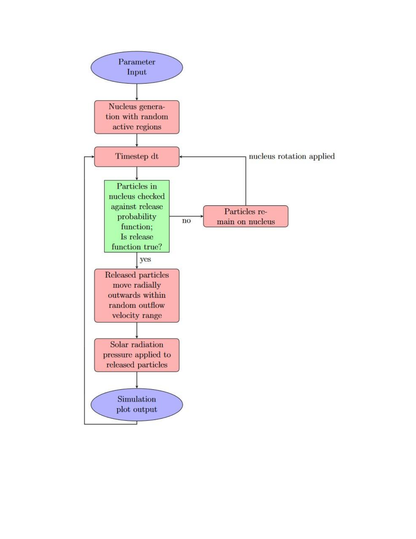
96
Figure 3.1 Flowchart for
model processes

97
3.2 Determining a limit for outflow velocity
One of the parameters that must be accounted for in the Monte Carlo model is the mean
outflow velocity of the radicals as they move outwards from the nucleus. Since there is no simple,
common factor amongst comets with regards to this behavior, we must try to determine it by
analyzing the positions of the emitted particles over time.
We use a similar method as [35] to constrain a velocity from our radial profile data. They
divided their enhanced division plots, obtained through narrowband photometry, into 10°
wedges, yielding 36 wedges in total. For each of these wedges that coincided with specific
morphological features in the coma, they examined the brightest points and tracked their relative
positions over the timespan of their observations. Due to the discrete, separated nature of our
fiber array spectrograph, as opposed to their CCD detector, we must use twelve 30° wedges to
ensure sufficient data are contained in each wedge. We tracked the radial position of the point
corresponding to the highest measured
𝑁𝑟𝑎𝑑
(where
𝑁𝑟𝑎𝑑
is the ratio between the column density
𝑁
and the modeled column density related to the projected radius from the optocenter,
𝑁𝑚𝑜𝑑𝑒𝑙
)
for constant features over the timespan of all of our observations for each night. The radial
positions for the carbon-bearing radicals, such as
𝐶
2 and
𝐶𝑁
, were grouped together to increase
the amount of available data.
These positions were plotted with respect to the difference in time from the first observation
for each usable 30° wedge. A line of best fit was found for each using linear regression, as shown
in Figure 3.2 on page 19. By comparing the regression slope parameters of each wedge for each
night, we can determine an upper limit on the mean outflow velocity of the particles from the

98
nucleus. This, in turn, can be used as a parameter to better model the outflow behavior of the
particles in our Monte Carlo simulation. This process is repeated for each identified active region
in the comet’s coma.
As the dust particles get farther from the nucleus, forces such as solar radiation pressure and
gravity start to dominate [28]. These additional parameters must then be accounted for and
calculated based on each simulated particle’s relative position to the comet nucleus and the solar
angle.
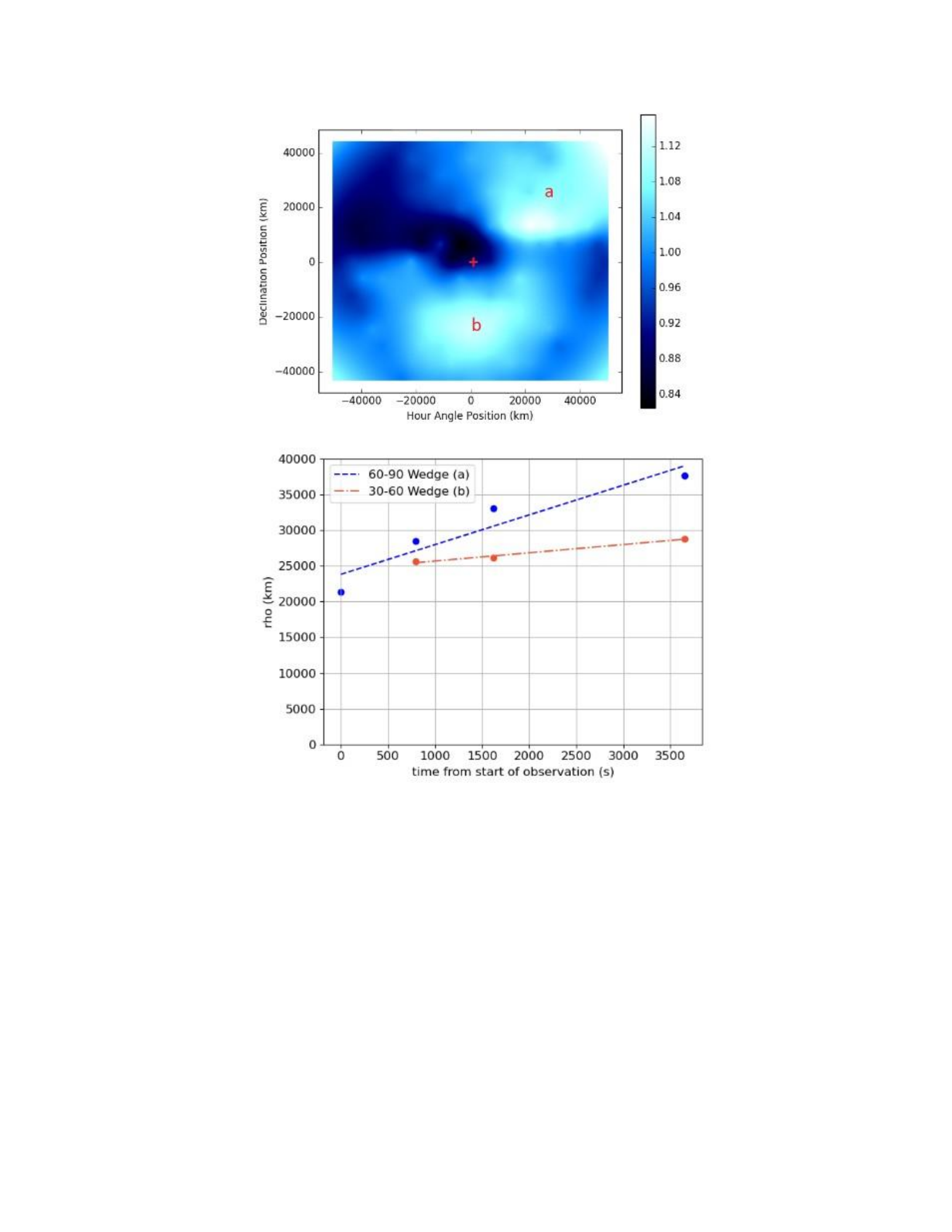
99
Figure 3.2
Outflow feature angular positions
Angular positions of detected features over the timespan of the observations of
Comet Garradd. The above figure depicts an example
𝐶𝑁
radial division map, and
the bottom figure shows the position vs time relation for
𝐶𝑁
over all observations.
The color bar scale on the upper map represents the column density of
𝐶𝑁
. The blue
line of the bottom figure represents feature (a), while the orange line represents
feature (b)

100
3.3 Comparing spatial concentrations
While a qualitative method of visually comparing the model results with enhancement plots
was established, a more quantitative approach was desired as well. A method outlined by
Vaughan [39] for analysis of comet data from the same IFU spectrometer was utilized, where the
enhancement plots were divided into a circle with symmetrical 60° wedges, centered on the
optocenter fiber. The fibers that were located in these position angle wedges were used to
calculate the concentration
ratio Ω,
! !−1
𝐴𝑧𝑖𝐷𝑖𝑣
𝑅𝑎𝑑𝐷𝑖𝑣
1 1
Ω= + + (3.2)
𝜎
2
𝜎
2
𝜎
2
𝜎
2
𝐴𝑧𝑖𝐷𝑖𝑣
𝑅𝑎𝑑𝐷𝑖𝑣
𝐴𝑧𝑖𝐷𝑖𝑣
𝑅𝑎𝑑𝐷𝑖𝑣
where AziDiv and RadDiv correspond to the weighted averages of the azimuthal division values
and the radial division values, respectively, for each fiber. A larger number of fibers within each
wedge allows for more accurate values of Ω, which is why 60° wedges are used, as opposed to
the 30° wedges used in the outflow velocity determinations. If a fiber resides exactly on a line
dividing the wedges, the concentration values are determined from the weighted average of two
symmetric fibers along either boundary of the wedge.
!−1
∑︁
𝐴𝑧𝑖𝐷𝑖𝑣
1
𝐴𝑧𝑖𝐷𝑖𝑣
2
𝑅𝑎𝑑𝐷𝑖𝑣
1
𝑅𝑎𝑑𝐷𝑖𝑣
2
Ω= +
(3.3)
2 2 2 2 2
𝜎
𝜎
𝜎
𝜎
𝜎
𝐴𝑧𝑖𝐷𝑖𝑣
,1
𝐴𝑧𝑖𝐷𝑖𝑣
,2
𝑅𝑎𝑑𝐷𝑖𝑣
,1
𝑅𝑎𝑑𝐷𝑖𝑣
,2

101
where the summation term is
1 1 1
+ +
𝜎
2
𝜎
2
𝜎
2
𝐴𝑧𝑖𝐷𝑖𝑣
,1
𝐴𝑧𝑖𝐷𝑖𝑣
,2
𝑅𝑎𝑑𝐷𝑖𝑣
,1
𝑅𝑎𝑑𝐷𝑖𝑣
,2
The average Ω values are then calculated for each wedge for each moment of observation.
The Ω
𝑎𝑣𝑔
values for each comet and observation are shown in Appendix A. This method is known
as
Welch’s Analysis of Variance (ANOVA).
Since the model does not simulate discrete fibers, the concentration is simply determined by
dividing the final output into 60° wedges and calculating the ratio of the number of particles in
each wedge with the overall total particles produced for the simulated comet nucleus. With
concentration values organized in this way, we now have an additional method of comparing the
model results with our observed enhancement plots after they have been initially constrained by
eye.

102
CHAPTER IV
RESULTS
The rotation of the comet is accounted for by setting a principal axis of rotation and including
a parameter for a change in angular position for set time-step intervals. Each time-step of the
model corresponds to the observations from the IFU spectrograph. For each time-step, the
particles within the active regions are checked against the release probability function. If they
pass the check, they are emitted radially outwards from the nucleus. If they do not pass, the
particle remains on the nucleus as it rotates in each interval. This process is repeated for every
time-step, with the emitted particles continuing their outward motion based on the outflow
velocity values. Non-released particles have a chance to pass the release probability check with
every step.
The outputs from the three-dimensional model are manually analyzed in a two-dimensional
grid to compare with the observable features as seen on the plane of the sky in the 2-D contour
plots. The rotational period of our coma model was adjusted until we were able to approximate
an acceptable fit to our observations obtained with the IFU. A sample output of the model is
shown in
Figure 4.1 on the following page.
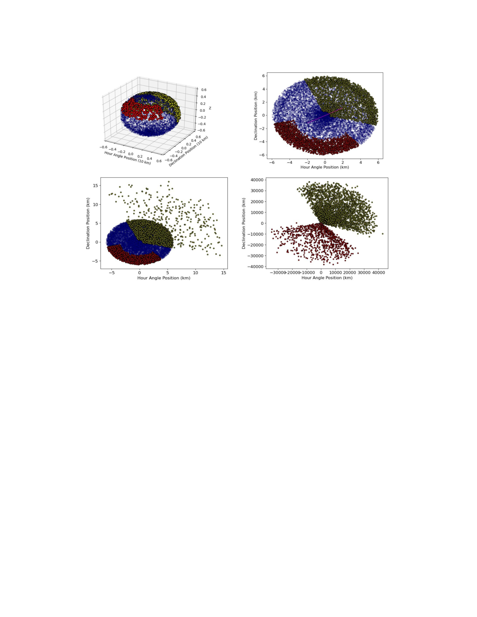
103
Figure 4.1
Sample nucleus of model
The top left image shows an initial setup in three dimensions, while the figure on the
top right depicts the respective setup in two dimensions, with the z-axis increasing
out of the page as the nucleus would be seen on the plane of the sky. The colored
circles represent the modeled particles. Inactive particles are blue, and the separate
active regions are shown in red and yellow. The two-dimensional plots are primarily
used to compare our results with the IFU observations. The bottom figures
represents subsequent timesteps.
4.1 10P/Tempel 2
Comet 10P/Tempel 2 is a Jupiter-family comet that was observed with the IFU spectrograph.
Tempel 2 has been a subject of much analysis from outside sources [23], making it a useful body
for comparison. The effective radius of the nucleus was determined to be 5.98 ± 0.04 km [24],
which is very large for a JFC. The rotation period was determined to be 8.950 ± 0.002 hours by

104
Knight et al. [21] at the time of its 2010/2011 perihelion approach. Furthermore, the period was
also determined to have increased slightly between perihelion passages in 1988 and 1999,
possibly due to systematic torque [23].
From our radial division maps for the carbon-bearing radicals of Tempel 2, we were able to
determine one large primary feature in the coma, as shown in Figure 4.2 on page 27. This area of
high column density was present in our observations from 2010 July 15 and September 13,
suggesting they are from the same active source. The angular position of the feature changes
very little between observations taken on each date, suggesting that the active region from which
it originates is located near a rotational pole. A similar feature was observed from the
𝑁𝐻
2 radial
division maps, though it is smaller in size.
Our Monte Carlo model was constrained to see if similar conditions could be observed from
the output. Thirty cases were produced from a parameter range, and the best fit was visually
chosen from among them. The parameters used for the final Tempel 2 simulations are shown in
Table 4.1 on page 26. The resulting images are shown in Figure 4.3 on page 28
Tempel 2 illustrates one of the main limitations with our model: working with a small number
of observations. Tempel 2 was observed with the IFU spectrograph for only two nights, both with
a small temporal range. Observation times are detailed in Table 4.2 on page 26. As comet
rotational periods tend to be at least several hours long, the available observations only offer a
glimpse at the spatial behavior for comparison with the simulation results. Furthermore, coma
plots from each enhancement date show only a single feature for all radical species, limiting our
ability to constrain our simulated plots by our usual visual standards.
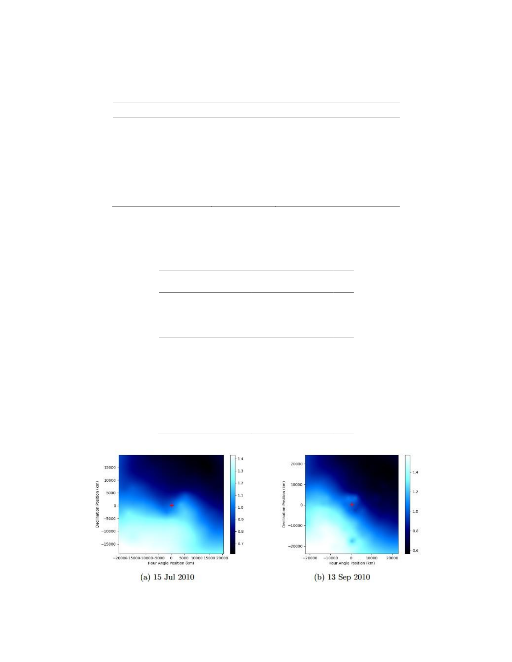
105
Table 4.1
Tempel 2 Model Parameters
Parameter Name
Value
Source
Radius
6 km
Lamy & Toth et al. 2009 [24]
Outflow velocity
0.6 km/s
Knight et al. 2012 [23]
Solar Vector Angle
109°
NASA Horizons
Rotation period
8 ± 0.5 hours
Custom parameter output
Active Area Fraction
34.3 ± .01 %
Random parameter output
Number of test cases
30
Result
Table 4.2
Observation times for Tempel 2
Observation Label
Start Time (UTC)
July 15 2010
278
08:39
300
279
08:48
600
280
09:03
900
September 13 2010
400
09:08
600
401
09:22
900
402
09:39
900
407
11:08
900
408
11:25
600

106
Figure 4.2
Radial division maps for
𝐶𝑁
in Tempel 2
ThelargeactivefeaturecanbeseeninthelowerleftinboththeJuly(left)andSeptember
(right) observations, suggesting little dynamic activity in this period of the comet’s orbit.
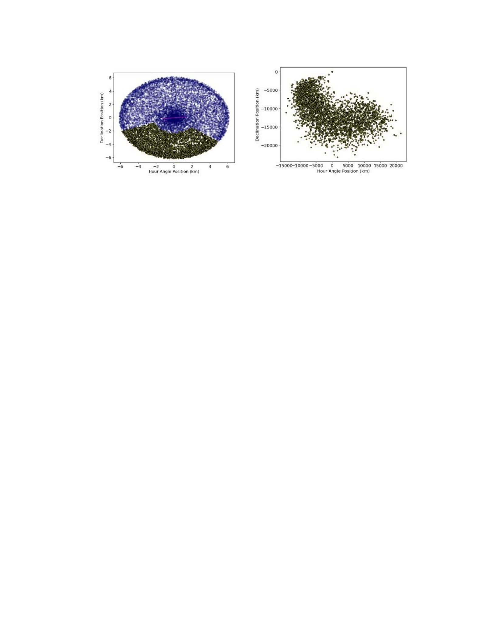
107
Figure 4.3
Plots for Comet Tempel 2 from the Monte Carlo model
The first image shows one of the earliest time-steps for the simulation, while the last
shows the resultant plot after a simulated passage of a little over 8 hours. The purple
line running through the nucleus in the left plot denotes the simulated primary
rotation axis, which is partially perpendicular to the plane of the figure.
4.2 C/2009 P1 (Garradd)
Our observations of comet Garradd showed a continuous feature present in the upper right
quadrant of the division maps for the carbon-bearing radicals, as seen in Figure 4.4 on page 32.
This suggests a relatively simple rotational mode for the comet, with the feature possibly
originating near the pole of the primary rotational axis. As such, we first tested our simulation by
inputting parameters from Garradd that were observed and also supported by other sources.
These are given in Table 4.3 on page 31. Due to the appearance of two features, a wider test case
of about seventy runs was required for a best-match simulation. Observation times are shown in
Table 4.4 on page 31, with each observation having a 600 second duration.
Figure 4.5 on page 34 shows comparisons between sample radial division plots and model
simulation results that most visually resemble them. The simulated total active area fraction was
generated as 49.5%, which would support our estimate that Garradd is a highly active comet. The

108
water production rates measured by Boissier et al. [6] suggests an active area fraction of at least
50%. One notable distinction from the model output is the lower concenctration of particles in
the feature in the bottom of the map for Figure 4.5b. This can be due to limitations with the
model, or it could indicate a more complex rotational mode for Garradd than was initially
assumed, as the feature is not present for the entire night of observations. It could also be due
to the fact that the simulated nucleus is stationary, with the only motion being due to rotation.
In reality, the comet is travelling through space as it orbits the Sun, so if an active jet were to
rotate away from view, we wouldn’t still be seeing all the residual outflow. All the carbon-bearing
radicals appear to have similar morphologies over our observation period, suggesting they
originate from the same source regions on the surface of the nucleus.
𝐶𝑁
is typically chosen for
primary visual comparison, as it has a better contrast in the coma compared to the other radicals
due to the strength of the violet band [23].
The concentration ratio of the active particles in the simulation shown in Figure 4.5 on page
34 match the Welch’s ANOVA wedge concentration spread, with the 0°, 240°, and 300° wedges
having the most activity across both. There is a difference in that the 0°-60° wedge in the model
has a slightly higher concentration than the 240°-300° wedge (27.5% and 28%, respectively) while
the relationship is reversed in the ANOVA concentrations found for
𝐶𝑁
, as shown in Appendix A.

109
Table 4.3
Comet Garradd Model Parameters
Parameter Name
Value
Source
Radius
5.6 km
Boissier et al. 2013 [6]
Outflow velocity
1-25 m/s
Mazzotta et al. 2016 [29]
Solar Vector Angle
139°
NASA Horizons
Rotation period
8 hours
Custom parameter
Active Area Fraction
49.5%
Random parameter
Primary Rotation Axis
𝜋
/6
Random Parameter
Number of test cases
75
Result
Table 4.4
Observation times for 2009/P1 Garradd
Observation Label
Start Time (UTC)
August 21 2011
944
02:45
946
03:12
948
03:46
950
04:16
952
04:47
958
06:18
960
06:50
962
07:21
964
07:53
966
08:26
968
08:59
August 22 2011
1028
02:53
1029
03:08
1034
04:34
1035
04:46
1039
05:52
1042
06:35
1046
07:40
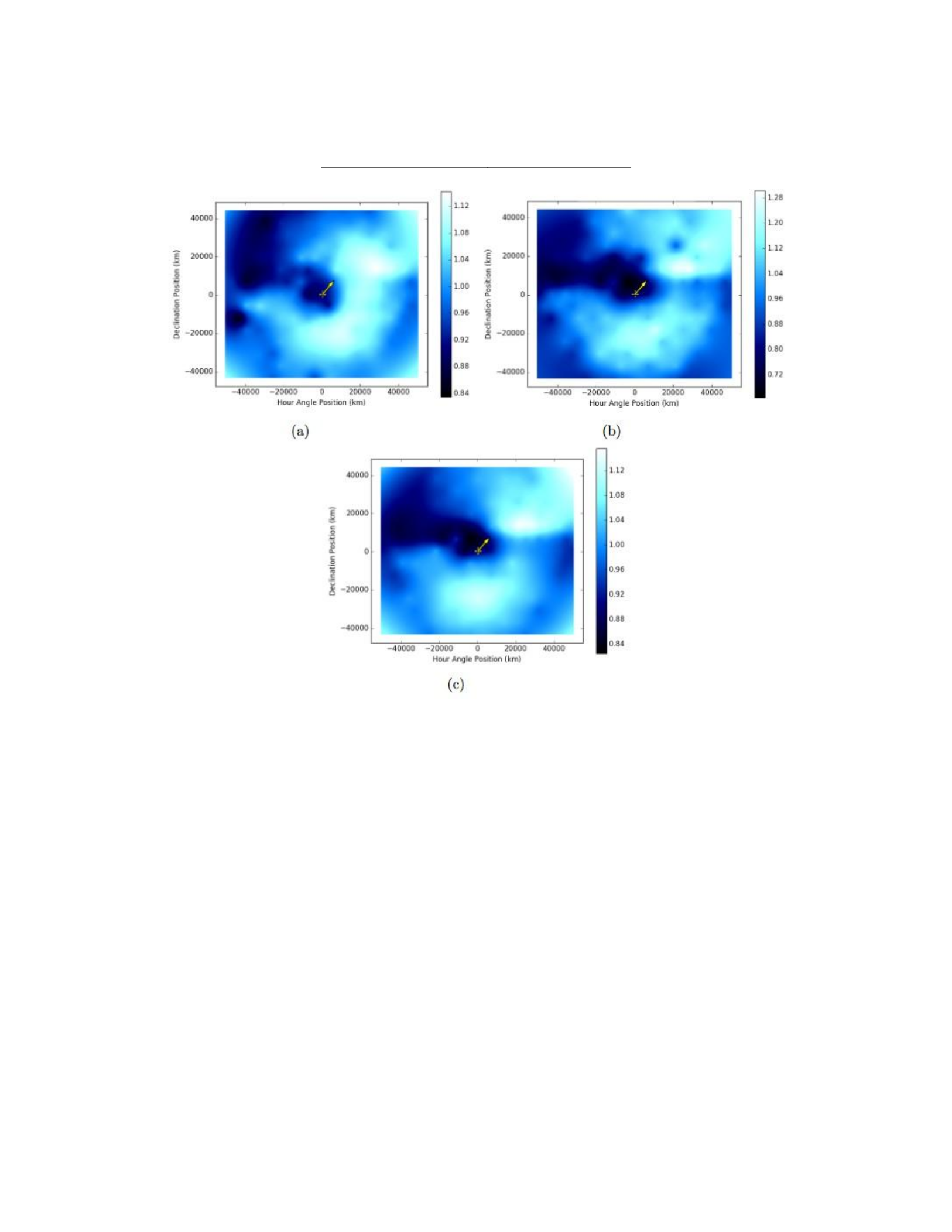
110
1051
09:01
1054
09:39
Figure 4.4
Radial division maps for Comet Garradd
Observations taken on the night of 2011 August 21 at 06:18 local time. The color bars
represent the column density of the detected radical. The white feature that can be
seen in the upper right is present for most of the night’s observations. This suggests
an active region rich in carbon-based molecules. The small yellow crosses represent
the locations of the optocenter, and the arrows represent the direction of the solar
vector. The solar vectors are pointing mostly out of the screen. The maps depict
𝐶
2,
𝐶
3, and
𝐶𝑁
, respectively.
While the spatial distributions of the carbon-bearing radicals are very similar to each other,

111
𝑁𝐻
2 exhibits a very different outgassing behavior for Garradd. Two coma features can be seen
opposite to each other on the top and bottom parts of the enhancement plots, similar in
appearance to an hourglass. This indicates that the features originate from two separate sources,
with the bottom source being different than the active region responsible for the carbon-bearing
radicals. These plots and their respective model simulation comparisons are shown in Figure 4.6
on page 35. The active particle spread most matches the ANOVA concentrations of the August 22
observations, with the wedges in the 60°-120° and 240°-360° regions showing the highest density
(14.4%, 24.2%, and 25.7%, respectively).
Both the
𝑁𝐻
2 and
𝐶𝑁
simulations had the same generating parameters, showing how they
could have separate morphology and possible source regions and yet arise from the same
rotational state. The model simulated a timespan of 292 hours with timesteps of 300 seconds.
Our best comparison plots were produced from an initial parameter for rotation period of 8 ± 0.5
hours. This is lower than values obtained from other authors. Farnham et al. [12] determined a
value of
10.4 ± 0.05 hours from lightcurve measurements, while Ivanova et al. [18] determined a period
of 11.1 ± 0.8 hours using a cross-correlation method of tracking a morphological feature over
time, similar to our own. Due to the wider number of available usable observations for Comet
Garradd, an additional method for checking the period was done by determining our own
lightcurve from the enhanced plots. The phase determined from this method also corresponded
with a period of 8±0.75 hours, which agrees with our model result. This suggests that this value
is at least consistent with our own observations. The lightcurve is shown in Figure 4.7 on page
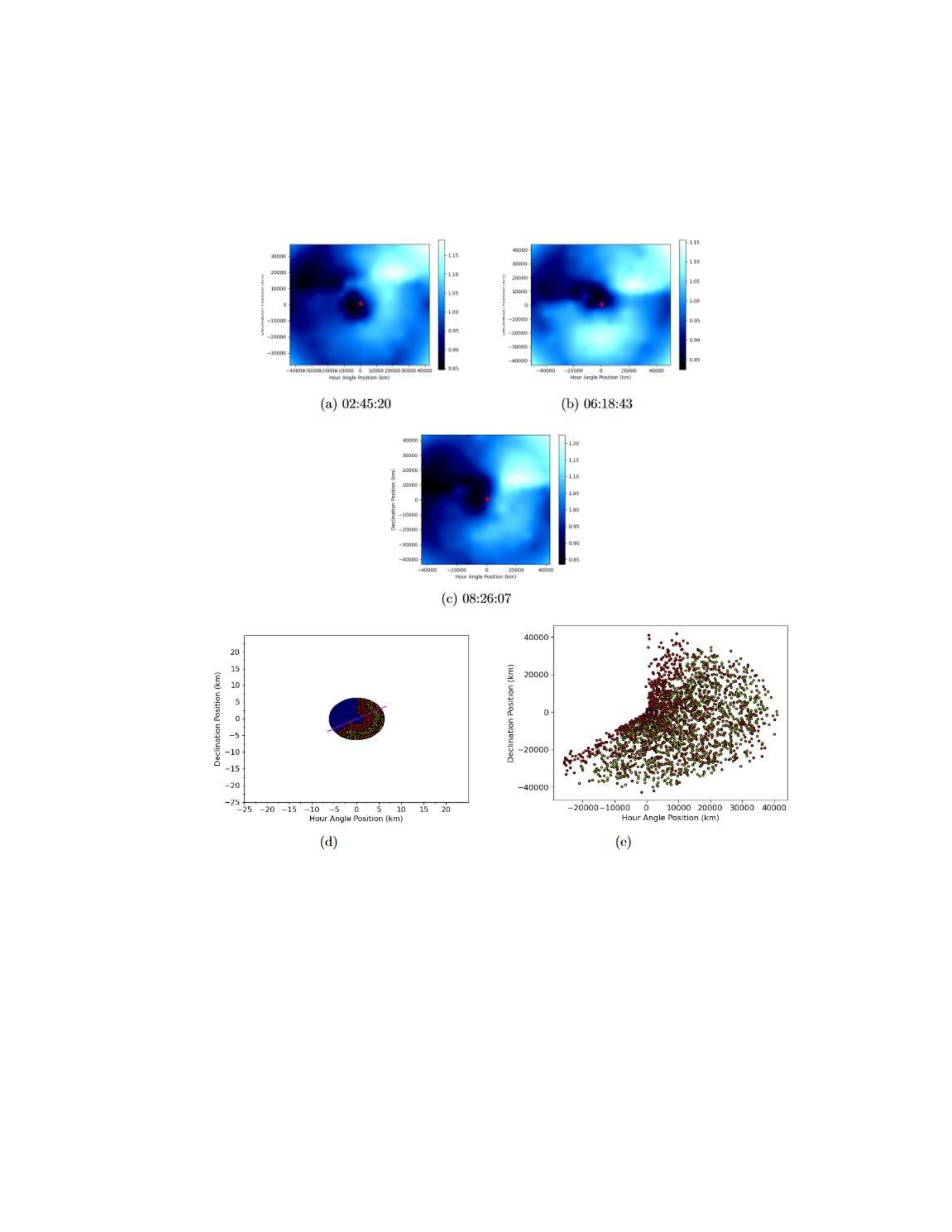
112
36. The discrepancy of our results from the others determined may be due to our different
observation methodology.
Figure 4.5
Garradd model CN comparison
Comparisons between radial division maps for
𝐶𝑁
in Comet Garradd and simulated
maps from the Monte Carlo model. The top three images show results over the night
of 2011 August 21 and their respective observation timestamps. The bottom row
shows maps randomly generated by the model that appear visually closest to the
enhancement plots, with the left being the initial generated nucleus and the right
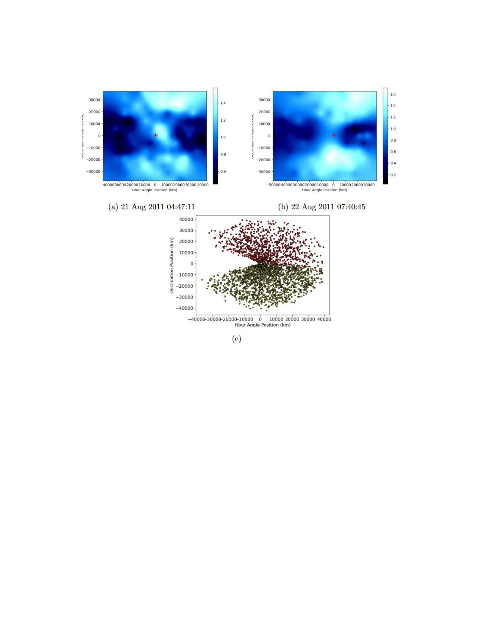
113
being the result after several timesteps. The purple line running through the nucleus
in the left plot denotes the simulated primary rotation axis.
Figure 4.6
Garradd model NH2 comparison
Comparisons between radial division maps for
𝑁𝐻
2 in Comet Garradd and simulated
maps from the Monte Carlo model. The top images show a sample observation over
two different nights. The bottom row shows a map randomly generated by the model
that appear visually closest to the enhancement plots.
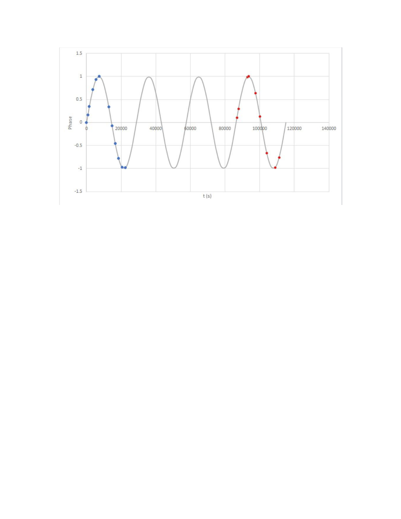
114
Figure 4.7
Garradd enhancement plot lightcurve
Lightcurve determined from our enhancement plots for our observations taken over
two nights. The blue dot represent observations taken on August 21, red dots
represent August 22. A phase (gray sine curve) was determined from similar
morphological features found in the enhancements of all radicals across both nights.
4.3 168P/Hergenrother
Comet Hergenrother presented unique challenges compared to our other comets. It is
another Jupiter Family Comet, whereas Garradd is a long-period comet, and thus likely has
different physical properties in terms of nucleus size and active area fraction, and a lot less is
known about Hergenrother as opposed to the other comets in this study. In terms of radicals,
Hergenrother was found to be extremely chemically depleted [33], allowing only viable
observations for
𝐶𝑁
. Only one bright feature can be seen in the
𝐶𝑁
maps, shown in Figure 4.8 on
page 41, so only one active area was set in the model. Fifty runs were required for Hergenrother

115
as well. The closest visual simulations are achieved by setting a rotation period parameter of 6.5
hours, and are shown in
Figure 4.9 on page 42. The other model parameters are shown in Table 4.5 on the following page.

116
Table 4.5 Comet Hergenrother Model
Parameters
Parameter Name
Value
Source
Radius
0.7 km
Custom
parameter
Outflow velocity
1-15 m/s
Custom
parameter
Solar Vector Angle
159°
NASA Horizons
Rotation period
6.5 ± 0.5 hours
Custom
parameter
Active Area Fraction
19.4 ± .01%
Random
parameter
Number of test cases
50
Result
Table 4.6 Observation times for
168P/Hergenrother
Observation Label
Start Time (UTC)
October 06 2012
1200
05:09
1201
05:35
1202
06:00
1203
06:55
1204
07:18
October 08
1307
02:57
1308
03:20
1309
03:42
1310
04:06
1314
05:39
1315
06:02
1320
08:01
October 09
1372
02:20
1373
02:44
1377
04:18

117
1378
04:42
1381
05:53
1384
07:01
1389
08:55
December 19 2012
1423
01:14
1424
01:48
December 20
1514
06:43
December 21
1577
01:15
1578
01:47
The active area fraction for the surface of the nucleus was 19.4 ± 0.01% for this best-match
simulation. This is much lower than the best-match runs for Garradd, which coincides with our
observation that Hergenrother is chemically depleted and less active compared to most comets
[33]. It remains to be seen if the depletion of Hergenrother, or its recent lack of detection near
its last expected perihelion [41], are related to the aforementioned fragmentation event. The
model constrainstherotationperiodforouranalysisof168Pto6.5±0.5hours.
Therearenomeasurements of Hergenrother’s rotation period from outside sources with which to
compare our result.
Due to the aforementioned chemical depletion, Welch’s ANOVA wedge comparisons were
done with our measurements of
𝐶𝑁
. The simulation output yield concentrations in the 0°-60°,
60°-120°, and 300°-360° wedges of 36.1%, 32%, and 28.5%, respectively. The actual ANOVA
calculations show higher wedge concentrations primarily in the 0°-60°, 240°-300°, and 300°-360°
regions, differing slightly from our model. This indicates that our model results may not align to
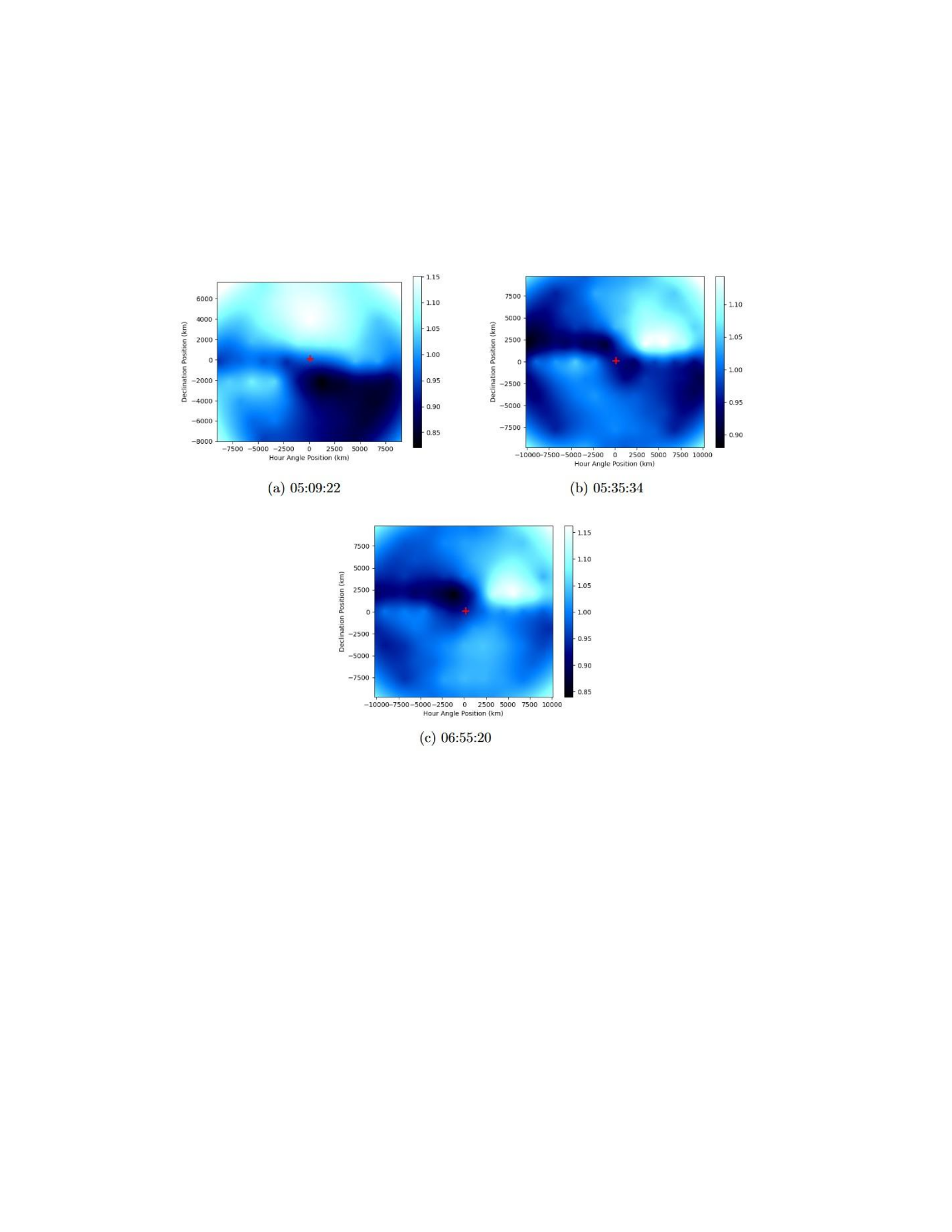
118
our observations with high precision. It is difficult to further constrain, as almost half of our
Hergenrother observations were dominated by a low signal-to-noise ratio, which can affect the
amount of usable fibers in the ANOVA calculations.
Figure 4.8
Hergenrother maps
𝐶𝑁
radial division maps for Comet Hergenrother on the night of 2012 October 6. Due
to the small interval of time coverage of the observations shown, the singular bright
feature in the upper right of each map moves very little between images.
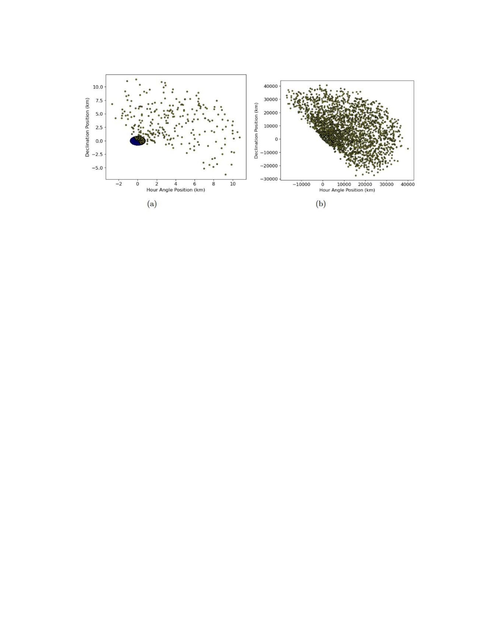
119
Figure 4.9
Hergenrother model CN comparison
Plots for Comet Hergenrother from the Monte Carlo model. The first image shows
one of the earliest time-steps for the simulation, while the last shows the resultant
plot after a simulated passage of about 290 hours. The purple line running through
the nucleus in the left plot denotes the simulated primary rotation axis.
CHAPTER V
CONCLUSION AND FUTURE WORK
The rotational period parameters that were set for the best-matching model results for each
comet were very close to the period constrained by either other sources or by visually tracking
the periods over multiple observations. The model also simulates possible active area fractions
for the comets and their approximate locations on the surface. These parameters are not well
constrained by observation alone, so these values can be of interest to other parties. The values
determined for active area fractions (34%, 50%, and 19% for Tempel 2, Garradd, and
Hergenrother respectively) suggests that long period comets like Garradd have higher active area

120
fractions than JFC’s such as Tempel 2 and Hergenrother, as they have experienced more
outgassing and perihelion passages.
Other methods of visually inferring rotational states of comets involves working with data
taken via multiple observations over a long timespan, typically months apart. The data for our
comets were only collected over a couple concurrent nights by the George and Cynthia Mitchell
IFU Spectrograph, limiting the long-term comparisons that could be done with our model. As
such our model results are only effective as comparisons with specific “snapshots" of the comets’
behavior. Further constraints could be placed with further observations, especially comparing
preand post-perihelion activity.
Future efforts will be spent on improving the model. Dust and gas are two very different
components of comet composition and exhibit different outflow behavior, especially beyond the
first few kilometers after release from the nucleus. Our reduced division maps from the IFU
spectrograph are based primarily on the gas located in the outer coma, and we must be cautious
in establishing a link to the dust outflow from the nucleus generated by the Monte Carlo model.
While both may come from similar jet sources, gasinteractions typically require parent-daughter
molecule interactions. A possible method of improvement would be to implement techniques
from a similar Monte Carlo model by Lederer et al. [25], in which trajectories of parent molecules
are tracked, and possible daughter decays are simulated by a exponential decay function. The
daughter molecules are ejected isotropically from the parent, and both are subsequently tracked
vectorially in the coma [25]. Additionally, the current version of the Monte Carlo model only
accounts for simple rotation around a primary axis. A more realistic model can be attempted by

121
accounting for more complex rotational states, such as precession and nutation, that have been
observed for other comets, such as Hartley 2 [4]. The comet’s translational motion as it moves
along its orbital path around the Sun could also be considered to eliminate residual outflow
between timesteps. Further checks must also be made to ensure uniqueness of our model
simulations, as multiple three-dimensional configurations of active area locations could
theoretically produce visually similar two-dimensional plots. The parameters of the model can be
adjusted accordingly as more information on our comets is corroborated and published by
outside sources.

