



Description of the Problem Area The complexity of cyberspace
The complexity of cyberspace makes cybersecurity one of the most significant challenges
of the enterprises of the 21st century. Ubiquitous cyber entities that integrate the cyber
environment with the real world increase the impact of cyber incidents on businesses. In order to
manage the impact of cyber incidents, cybersecurity risk analysis becomes the primary tool.
According to Kaplan and Garrick (1981), risk analysis is conducted by answering three
questions:
•What unwanted risk scenarios can occur?
•What is the likelihood of these incidents occurring?
•What is the impact if these incidents occur?
A generic formula for quantitative risk analysis is determined based on these questions.
Based on the generic risk formula, the risk is a set of triplets:
𝑅𝑅 = {< 𝑆𝑆𝑖𝑖, 𝑃𝑃𝑖𝑖, 𝑋𝑋𝑖𝑖, >}
where 𝑖𝑖 = 1,2, . . , 𝑁𝑁
𝑆𝑆𝑖𝑖 is a scenario identification,
𝑃𝑃𝑖𝑖 is the probability (likelihood) of an incident to occur,
𝑋𝑋𝑖𝑖 is the impact in a scenario when it occurs, and
𝑁𝑁 is the number of scenarios considered (Kaplan & Garrick, 1981).
This generic formula also applies to cyber risk analysis. Likelihood and impact
assessment are critical components of risk analysis. Likelihood assessment includes efforts to
estimate the probability of such incidents to occurs, for example, based on the historical data.
Impact assessment consists of models that aim to calculate the consequences of possible damage

on the assets and data, loss of intellectual property, costs caused by business interruption, and
penalties. Such risk management activity by likelihood and impact assessment helps provide
insights on the prioritization of risk events. Prioritization assists decision-makers in investing in
the most effective and efficient way. Models of risk quantification also establish a shared
communication language among technical cybersecurity experts and top-level management
members of an enterprise so that technological and business aspects of cybersecurity can be
coordinated accordingly (Bahsi et al., 2018).
Problems in Cyber Risk Assessment
There are several limitations of the current cyber risk analysis methods. Cyber risks are
often considered an information technology problem rather than a vital part of enterprise risk
management (Moore et al., 2015; Tatar et al., 2020) that has been conducted comprehensively.
Existing cyber risk analysis methods assess risk mostly at the asset level (e.g., via software
quality assurance, vulnerability analysis, intrusion detection, malware analysis), to some degree
at the organization level (i.e., business processes), and very few at the ecosystem level (i.e.,
supply chains) (U.S. Department of Homeland Security [DHS], 2018). Beyond existence,
integrating asset-level cyber risk analysis with higher levels is a limitation of the current
likelihood and impact assessment methods.
Another deficiency of the cyber risk analysis methods is the insufficiency of the utilized
metrics to support investment decisions, including cyber insurance. Qualitative metrics and
operational terms are often used as cyber risk indicators rather than quantified financial measures
that guide investment decisions. Qualitative or operational cyber risk metrics lead to, firstly, a
lack of understanding for organizational leaders, secondly, a reluctance to appreciate the

significance of cyber risks. This issue was stated in the Strategic Plan for the Federal
Cybersecurity R&D Program: “There is no scientific basis for cost risk analysis, and business
decisions are often based on anecdotes or unquantified arguments of goodness” (Executive Office
of the President, 2011). Besides this, the lack of quantification of how investments in specific
controls change risk levels (i.e., measurement of the effectiveness of planned or implemented
controls) is another limitation of the current cyber risk analysis methods (Tatar et al., 2020).
To partially address the limitations mentioned so far, Functional Dependency Network
Analysis (FDNA) (Garvey & Pinto, 2009) was adapted to the domain of cyber risk analysis by
Tatar (2019) with a deterministic approach (named as FDNA-Cyber). FDNA was modified
significantly to model the cyber impact propagation within the layers of an enterprise and
amongst different enterprises (Tatar, 2019).
Significant modifications to FDNA include expressing impact as a function of loss of
confidentiality, integrity, and availability and new mathematical dependency relations reflecting
the nature of cyber dependencies. However, characteristics of some cyber risk sources have a
probabilistic behavior that cannot be modeled effectively with a deterministic model. For
example, the strength of dependency between two functional nodes might be a specific statistical
distribution. Analyzing the effects of such uncertainty is a limitation of the current methods.
Moreover, the impact and likelihood of a risk scenario can differ in time. Only a few studies
cover the temporal change of strength and criticality of dependencies and the associated risk
value (Xu & Hua, 2017). Current methods of impact propagation modeling are limited since they
can only provide a snapshot.

Communication of cyber risks among people from different roles within an enterprise is
problematic since tactical, operational, and strategic level decision-makers handle cybersecurity
in various ways. The tactical level is concerned with the number of vulnerabilities within the
systems and possible defensive actions, while operational level decision-makers consider legal
and organizational constraints. On the other hand, strategic level managers tend to consider
effects on the operation of the overall business. This situation causes a gap in communication of
cyber risks. Risk quantification models help bridge this gap by gathering people from different
backgrounds over a language that everyone may understand. For example, attack graphs are used
as a tool to analyze the likelihood of possible attacks; however, it is still a limitation to translate
the outcomes of attack graphs to organizational risks and economic indications as the strategic
level decisionmakers can benefit. Probabilistic models still need improvements to integrate
tactical level decision making with the operational and strategic level decision making.
Another limitation is that the Bayesian attack graph approach, a probabilistic attack graph
representation, requires input that is general enough to be adopted by enterprises in different
sectors with a reasonable level of effort along with the conventions of how to adapt the methods
for the requirements of a specific enterprise environment. Researchers commonly use the
vulnerability characteristics provided by National Vulnerability Database for this purpose (Shetty
et al., 2018). However, the integration still requires to be more convenient for adaptation to the
environment of each enterprise.
In order to address these limitations of the current studies, the developed cyber risk
analysis method employs probabilistic attack graphs, which are based on known vulnerabilities in
computer software and network topologies. The risk assessment capabilities are augmented in the

attack graph using Bayesian Networks (Tatar et al., 2020). The developed cyber risk analysis
model also leverages the FDNA-Cyber method (Tatar, 2019) and integrates it with probabilistic
attack graphs.
Enterprise Architecture and Impact Propagation
Enterprise architecture for impact analysis consists of functional nodes of an enterprise
and dependencies among these nodes (Jacobson, 2011; Tatar, 2019). This representation is also
called an impact graph since it is represented as a graph by nodes and their dependencies and is
used to analyze impact propagation. Enterprise nodes are categorized as three layers according to
their characteristics:
1. Asset Layer consists of the ICT hardware and software that runs on the hardware.
Servers, workstations, routers are examples of assets.
2. Service Layer includes the services such as e-mail, internet, and security.
3. Business Process/Mission Layer consists of an organization's primary capabilities that
enable generating value or revenue; when interrupted, the organization suffers by
losing revenue or capability. An example of a business process for an e-commerce
company is selling goods on its website.
Impact propagation among the nodes of an impact graph is assessed depending on two
types of dependencies. Horizontal dependencies (i.e., intra-layer dependencies) are the
dependency relationships within a layer. Vertical dependencies (i.e., inter-layer dependencies)
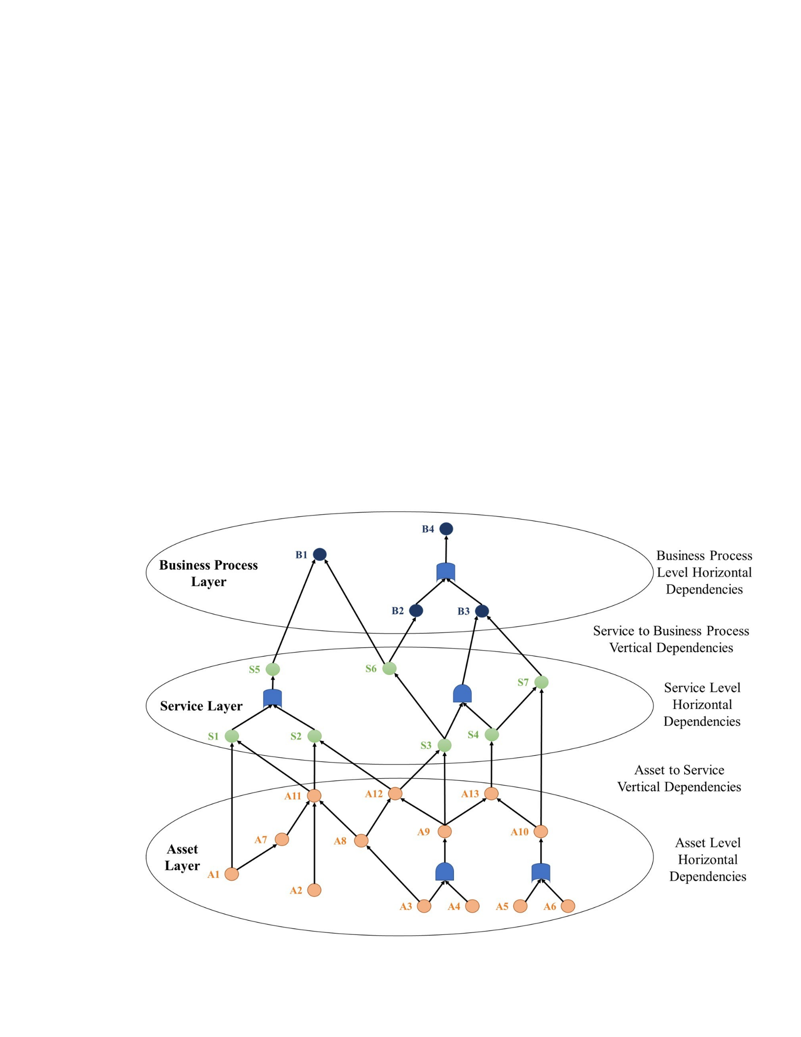
represent the dependency relationships among the nodes of different layers. An example impact
graph with three layers of an enterprise and the dependencies is presented in Figure 1.
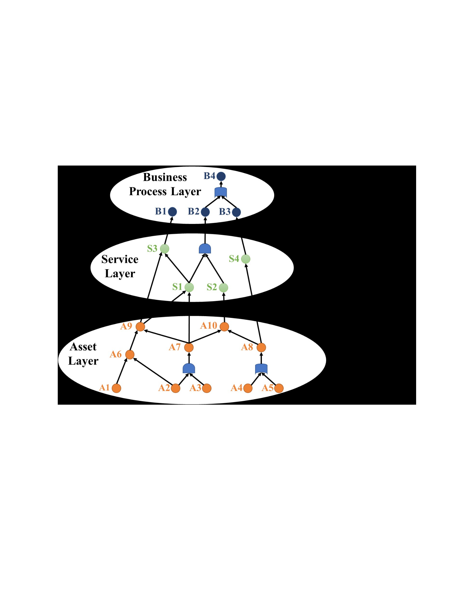
Figure 1.
Three-layered impact graph for an enterprise
Challenges in Cyber Risk Assessment
Researchers who tried to address some of the described problems in the cyber risk
analysis literature have faced some challenges while developing practical risk assessment
models. These challenges are not only some difficulties to overcome but also some key features
for a comprehensive cyber risk analysis model. These challenges can be summarized as:

1. A realistic asset targeting modeling from an attacker’s perspective is required to
consider the defenses from a hostile point of view to identify critical attack paths
and critical assets to defend.
2. Thousands of known vulnerabilities exist; however, not all known vulnerabilities
have an exploit against them. Moreover, some of the vulnerabilities within an
enterprise network lie behind the multiple layer defense mechanisms so that they
are not exploitable unless the preceding attack steps are successfully conducted.
This suggests that threat levels of different vulnerabilities vary.
3. A standard way of quantifying likelihood and impact is required to establish an
effective communication approach regarding vulnerabilities that keep everyone on
the same page and prevent misunderstandings.
4. A model to be developed needs to be able to be tailored based on the
organizational environment. There should be a balance between the
generalizability and the specificity of the model. Decision-makers of an enterprise
should be able to adopt the model by modifying it according to their
environmental needs.
5. Communication issues among different levels of management should be resolved
by providing a way to bridge the gap. This requires conducting the cyber risk
assessment not only at the asset layer but also at the service and business process
layers. How the impact would propagate from the asset to the business process
layer should be considered to bridge the gap between tactical and strategic level
management.

6. Assessing cyber risks in terms of loss of business can be conducted by translating
the technical cybersecurity language into business management jargon. This can
be conducted by assessing the impact caused by security issues of some ICT
assets on the operability of the business processes of the enterprise. This challenge
should be considered with the previous challenge to provide a feasible solution for
the issue. 7. Cyber risks are siloed and considered a technical problem rather than
a part of Enterprise Risk Management that is conducted comprehensively.
Commonly, an enterprise does not conduct much about cyber risks other than
employing a security scorecard approach and minimally complying with the
industry or regulatory requirements. In a field where historical data scarcity has a
crucial impact, organizational tailored cyber risk assessment approaches are
critical. Combining the key features of the solutions to respond to the previous
challenges, a model can be developed to comprehensively address cyber risks as a
part of Enterprise Risk Management.
Knowledge Gap and Contributions of the Study
Even if some studies in the literature have tried to address these challenges, not all of
these key features were successfully implemented on a cyber risk assessment model. The
following significant knowledge gaps still exist in the literature:
1. Integration of attack propagation and business impact assessments of cyber
incidents,
2. Lack of probabilistic impact propagation models for a multi-layered enterprise
functional dependency network,

3. Limitations of time-dependent and enterprise-specific adaptability of a generic
vulnerability scoring system for estimating the likelihood of attack success, and
4. Lack of temporal models that makes analyses inefficient since they only take
snapshots of the status of the enterprise system.
The goal of this research is to build a probabilistic cyber risk analysis model that relates
attack propagation with risk (i.e., impact and likelihood) propagation through internal
dependencies and allows temporal analysis.
The contributions of the developed research are:
•Attack propagation model that adapts vulnerability scoring that
o Is customizable for organization, and o Considers temporal
aspect.
•Impact propagation assessment model that o Is probabilistic o
Allows temporal aspect.
•Integrating attack propagation and impact propagation
assessment.
Research Question and Objectives
Research Question: What probabilistic cyber risk analysis model can be developed by
considering cascading impacts through internal dependencies (e.g., vulnerabilities of assets to
business processes) and allowing temporal analysis?
In order to build a model that answers this question, four major research objectives should
be achieved.

Objective 1: Development of a customizable attack propagation model that adapts
vulnerability scoring by employing Bayesian attack graphs
Objective 2: Development of a probabilistic impact propagation assessment model by
considering dependencies and allowing temporal aspect
Objective 3: Development of a model integrating attack propagation and business impact
propagation to calculate economic impacts of cyber risks of an enterprise
Objective 4: Validation by simulation
Table 1 presents how the challenges, knowledge gaps, and the developed research can be
mapped for clarification.

11
Table 1.
Mapping challenges, knowledge gaps, and research contributions
Challenges Knowledge Gaps Research Contribution Tool
1. Target modeling from attacker’s perspective
Customizable Attack propagation
model that adapts
2. Vulnerability risk ranking
3. Standardized risk quantification
1. Limitations of time-dependent
and enterprise specific likelihood
estimation for attack success vulnerability scoring by enhancing
CVSS integration into Bayesian
attack graphs
Attack
Graph
4. Customizable model
5. Bridging levels of management 2. Lack of
temporal
models
3. Lack of
probabilistic impact
propagation models
Probabilistic impact propagation
assessment model that allows
temporal aspect
Impact
Graph
6. Cyber risks as business loss
7. Vital & comprehensive element of
Enterprise Risk Management 4. Integration of likelihood and
business impact assessments
Integrating attack propagation and
business impact propagation Both

12
As shown in Table 1, research contribution regarding attack propagation fills the first
literature gap by using attack graph as a tool that employs Bayesian attack graph algebra. This
research contribution also covers the first three challenges and partially covers the model
customization challenge (Challenge 4).
The second main research contribution regarding impact propagation fills the second and
third literature gap by using impact graph as a tool that employs Functional Dependency Network
Analysis algebra (More details provided in Chapters 2 and 3). This research contribution also
covers challenges 5 and 6 and partially addresses the model customization challenge (Challenge
4).
The third main research contribution regarding the integration of attack propagation and
business impact propagation covers the fourth gap within the literature and the last challenge.
Contribution to the Engineering Management Field of Knowledge
Risk Management
Its Use for Enterprise Decision Makers. The developed model can be employed to
quantify the risks of an enterprise by considering both from the attackers’ and the defenders’
perspectives. Such analyses help make well-informed decisions instead of depending on the
feelings of the decision-makers based on their experience. Using the developed model, the
decision-makers can simulate various cyber-attack scenarios to benchmark the economic impact
of different cybersecurity investments on the enterprise's business processes. Moreover, the
developed model help analyze the cyber risks of the enterprise against a diverse set of attacker
groups such as Advanced Persistent Threat actors.

13
Its Use for Insurance Companies. In general, it can be challenging to calculate an
insured’s Total Insurable Value (TIV) for the purpose of pricing cyber coverages. Outputs of this
research address this challenge from an Economic- Functional Approach.
Particularly for property insurers, the output of objective 2 (i.e., application of impact
graph) can be used to strengthen their estimation of an insured’s Property Value as the first part of
the TIV. In the advent of the trend where data is considered a property, the valuation and
inclusion of data-as-a property into TIV can be facilitated by knowing the economic value of data
on the insured’s operations. Eventually, this will affect insurance pricing regarding replacement
and repair of data-as-a-property if such is covered under policies.
The output of objective 3 (i.e., integrating attack and business impact propagation
models) can be used to strengthen the estimation of an insured’s Time Element (TE) as the
second part of the TIV. Depending on various cyber incidents or scenarios covered under policies
(e.g., ransomware, Distributed Denial of Service), the potential ripple effects and subsequent
duration of disruption to the operation of the insured may depend on functional dependencies
among insured and noninsured assets. Awareness of the functional dependencies and resulting
ripple effects within and outside an individual primary insured (e.g., upstream cloud service and
downstream tertiary insured) may help in determining other factors that affect pricing, e.g.,
qualifying cyber events, exclusions, waiting periods, and limits – both at the individual insured
and for a portfolio of insured who have some degree of interconnectedness.
Summary

14
The goal of the developed model is to provide a holistic cyber risk assessment approach
that integrates calculation of attack propagation with asset layer to business process layer risk
propagation.
Two primary outcomes of the developed model are as follows:
•Using this model, business process operability loss can be simulated for various
scenarios.
•Probabilistic and temporal analyses can be conducted using the simulation model.
CHAPTER 2
LITERATURE REVIEW
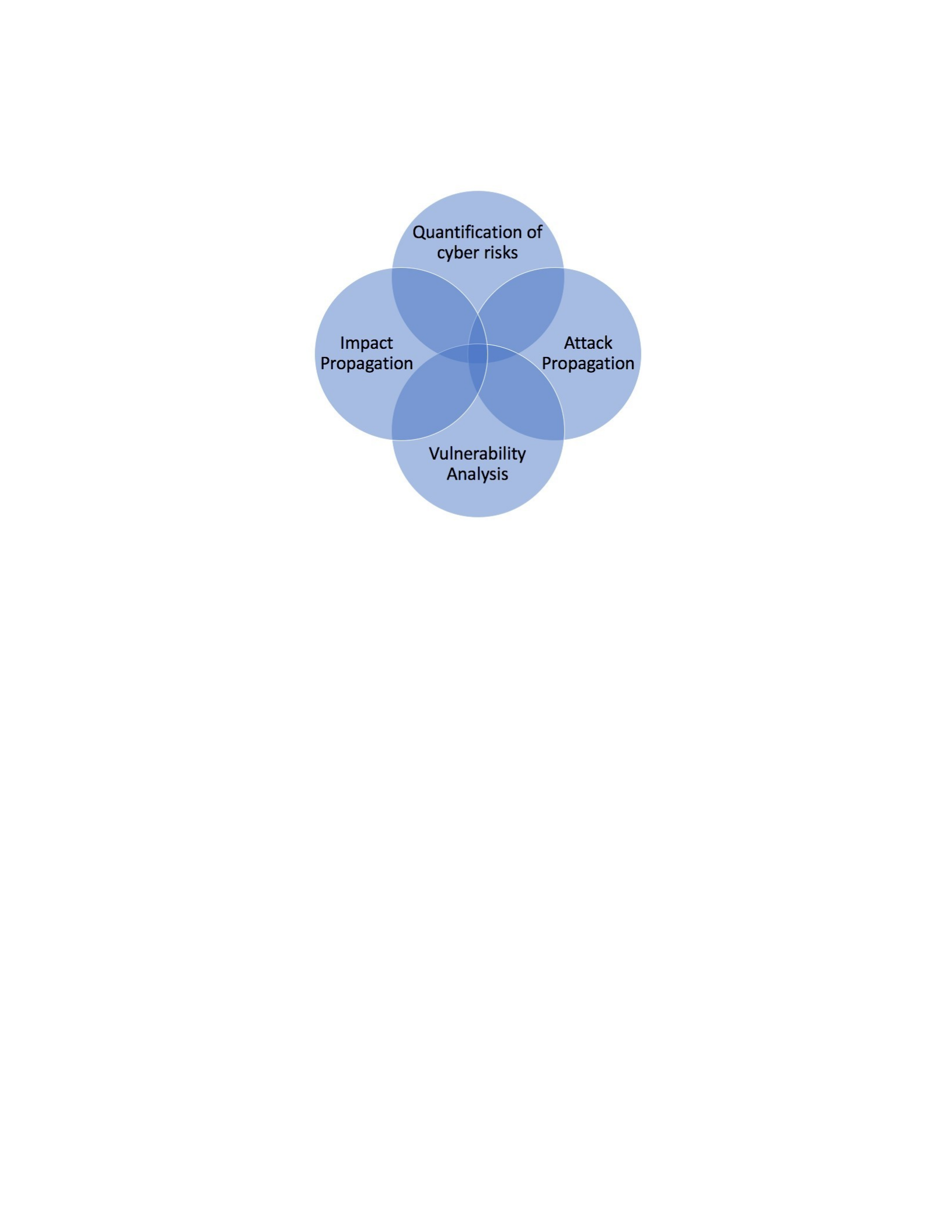
The literature relevant to the prosed research clusters in four main areas (Figure 2):
1. Quantification of cyber risks,
2. Vulnerability analysis,
3. Attack propagation, and 4. Impact propagation.
Figure 2.
15
Four main clusters of literature
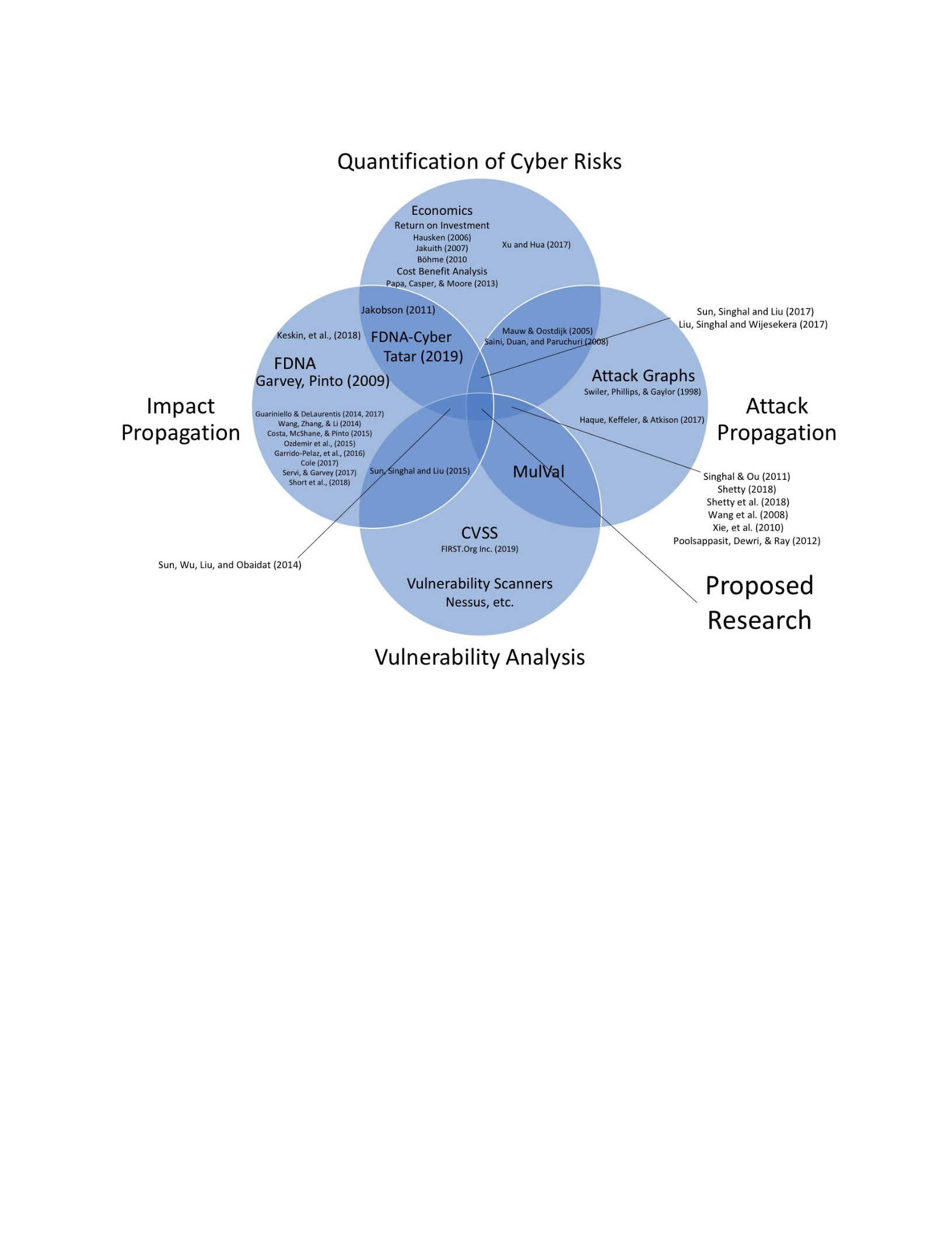
The developed research takes place at the intersection of these four main areas. In this
chapter, various studies were reviewed. While most of the reviewed studies fall into only one
area, some studies combine the concepts of two or three areas (Figure 3). The following sections
of this chapter provide more details on the relevant studies.
Figure 3.
Literature map
16
In the first section of the relevant research summary, the deficiencies and necessities of
the current cyber risk analysis methods are examined from an economic and general perspective.
In the following sections, the major research that specifically employed similar methodologies
such as attack graphs, CVSS, and impact graphs is surveyed to figure out the novelty and
contribution of this study. Since FDNA is considered an integral part of the developed model for
impact graph analysis, more depth on FDNA related research is presented in the last section of
this chapter.
Quantification of Cyber Risks

17
Being a relatively new risk source, models to quantify cyber risks are not well developed;
therefore, cyber risk management in most businesses depends on qualitative assessments. With
the increase in the economic consequences of cyber incidences, the importance of quantification
of cyber risks has been increased. In this section of the literature review, the economic aspects of
cyber risk research, along with its connection with the insurance industry and other approaches to
cyber risk analysis, are presented.
Economic Aspects of Cyber Risk and Insurance
Cyber risk has become a top agenda item of businesses across the world and is listed as
one of the top three global risks with significant economic implications for businesses (Allianz,
2016). The cybersecurity rating of companies is an emerging decision-making factor in
investment assessments (Bloomberg, 2014). Chief Information Security Officers (CISO) started
having more critical roles in the executive boards since they are responsible for securing
organizations from cyber threats and need to provide strategic guidance to other board members,
specifically regarding the effectiveness and efficiency of cybersecurity investments. The
executive board depends on CISOs for insights regarding the organization's cybersecurity posture
in a language they can understand – costs, risks, and benefits – and how cyber risk maps to
dollars instead of the latest purchase of an IT security product (Rifai, 2017). In order to transform
cyber risk management from a technical issue to a business issue, cyber risk has to be quantified
as monetary value eventually. As well, the valuation of cyber risk will ultimately be integrated
into Enterprise Risk Management frameworks (Ruan, 2017). Consequently, cyber risk
management has become an emerging and vital part of enterprise risk management.

18
According to Dynes et al. (2005), cyber risk management in enterprises was mainly
conducted by qualitative methods. Some researchers attempted to quantify cyber risks to compare
cyber investment options. Traditional techniques were applied for risk quantification, such as
Return on Investment by Hausken (2006), Jakuith (2007), and Böhme (2010) and Cost-Benefit
Analysis by Papa et al. (2013).
Research on the topics of the economics of cyber risk and cyber insurance has grown
exponentially since 2010. This growth highlights the increasing relevance of the subject from
both a practical and an academic perspective (Eling & Schnell, 2016). In order to respond to
cyber threats via risk transfer, the cyber insurance market is also emerging worldwide, including
the US. According to AON (2017), the global stand-alone cyber insurance market had $1.7
billion in annual gross written premium in 2015 and increased to $2.3 billion in 2016, with 70
insurers exist that offer a standalone cyber product in the US. The US's total net written
premiums of cyber insurance policies are $1.94 billion in 2018 and are expected to reach $20
billion by 2025 (Bernard, 2020).
Existing articles for cyber risk analysis from an insurer perspective emphasize the
following challenges (Eling & Wirfs, 2016): lack of data and modeling challenges, the
complexity and dependent risk structure, adverse selection and moral hazard issues, and necessity
of a scenario-based analysis of potentially huge losses from the breakdown of critical
infrastructures. From the insured’s perspective, the monetary value of the residual should be
calculated to decide how much residual risk should be transferred to insurers. From insurers' and
reinsurers' perspectives, profiling risk exposures and quantifying accumulated risk to the

19
portfolio of entities caused by using a shared technology platform (such as cloud computing) and
hyper-connectivity in the digital supply chain is a necessity (Eling & Schnell, 2016).
One of the major problems of actuaries working in the insurance sector or enterprise risk
management is the availability of valuable historical data for cyber risk. Almost all security
companies keep incident and loss data as proprietary to have a competitive advantage (Ruan,
2017). Subsequently, there is insufficient data to employ statistical methods and mathematical
models for appropriate calculations and predictions. To cope with the data scarcity, some have
suggested avoiding using classical stochastic modeling and instead rely on scenario approaches
(Lloyd’s, 2015). For Rakes et al. (2012), employing expert judgment to define worst-case
scenarios and estimate their likelihood for high-impact IT security breaches is a more efficient
approach. Even more so, a fast-changing technology environment requires a modeling approach
that dynamically measures risk (Eling & Schnell, 2016).
Other Approaches on Cyber Risk Analysis
Cyber risk analysis methods commonly put more emphasis on technology and less on
people, processes, and socioeconomic risk factors (Spears, 2005) during the previous decade.
Recent major risk assessment approaches such as ISO/IEC 27002 are designed based on security
control domains and focus more on an asset’s security posture while ignoring its preparedness
towards a set of high-risk loss scenarios (Ruan, 2017).
One of the most recent articles proposes a new method to quantify cyber risk by adapting
medical risk calculation (MicroMort) and financial risk calculation (VaR) methods (Ruan, 2017).
Four types of risk factors have been identified: technological, non-technological, inherent, and
control factors. Inspired by MicroMort and VaR, BitMort and Hekla have proposed to measure

20
the cost-effectiveness of control factors, reflect an entity’s willingness to pay to reduce cyber
risk, cyber risk limit, and cyber risk appetite. The proposed quantification of the cyber risk
method is innovative and provides a significant contribution to the literature. However, it does
not consider vulnerabilities that nodes pose in a network or functionalities of those nodes and the
ripple effect.
Some studies in the literature conduct surveys with CISOs to explore the rationale and
motives while making decisions on cybersecurity investments. Libicki et al. (2015) found that it
is a challenge for CISOs in government and military organizations to find support from the
stakeholders and other management personnel. Cavusoglu et al. (2015) found that coercive and
normative pressures within the organization significantly affect information security control
resources. Moore et al. (2015) suggest that most executives believe that their organization
sufficiently invests in cybersecurity; however, this causes them to spend resources on improving
the protection against new threats. Additionally, they found out that even if the organizations
follow industry compliance for cybersecurity, most of them do not conduct quantitative
cybersecurity risk management by examining the dollar outcomes of the security investments.
Xu and Hua (2017) developed a framework for modeling and pricing cybersecurity risk in
a study. The framework has three components: epidemic models, loss functions, and premium
strategies. This framework employs stochastic processes (Markov and non-Markov), utilizes the
copula to obtain the dependencies, and utilizes Monte Carlo simulations to assess the security
level of networks and the number of incidents, the likelihood of node infection, and the final
losses. Even though this study addresses the impact on the network, however, nodes on the

21
network may be different in terms of vulnerability, interdependency, and functionality.
Furthermore, it does not include the vulnerability levels of the nodes.
Petri Net is another method used to analyze information flow within systems (Peterson,
1979). It helps analyze the system by modeling in a graphical representation and establishing
relationships by providing a probabilistic approach (Murata, 1989). It is widely used in safety
analysis, accident modeling, reliability studies, and risk assessment in various fields, such as
nuclear industry, manufacturing processes, industrial storage systems, emergency response, and
critical infrastructure operations (Vernez et al., 2003; Henry et al., 2010).
Some studies employed attack trees and attack graphs to structurally identify and assess
attack probabilities on a system (Mauw & Oostdijk, 2005). Saini et al. (2008) integrated risk and
cost values to each attack vector in the attack tree to make more realistic security threat
evaluations.
The next section of the literature review provides depth into attack graphs.
Attack Graph
There are hundreds of nodes in a typical enterprise Information and Communication
Technology (ICT) network (e.g., computers, routers, switches storage devices). Counting the
number of vulnerabilities of the components of these networks is not an efficient and effective
way of quantifying the cyber risks. Many of these vulnerabilities are not initially exploitable in
such a network since a multi-layered defense prevents attackers from directly reaching the
targeted host. Moreover, some of the vulnerabilities are not exploitable at all. In order to reach
the target host, the attackers need to examine the network topology and successfully exploit the
vulnerabilities existing on each node on the path, taking them to their target (Tatar et al., 2020).

22
From a defense perspective, information security personnel need to consider the network
from the attackers’ perspective to identify the critical components, reveal the possible attack
paths, and determine the weakest links within the network. Estimating the more probable attack
paths improves risk management and supports investments in more efficient cybersecurity
products and services (Tatar et al., 2020).
An Attack Graph is a graph-theory-based formalism that helps visualize and analyze
cyber-attacks that combine exploiting multiple vulnerabilities (Swiler et al., 1998).
Securityrelated configurations of the system are shown along with the existing vulnerabilities on
a graph. Exploiting the vulnerabilities causes changes in system status (Singhal & Ou, 2011).
Meanings of nodes and edges and what they represent may change according to the definitions
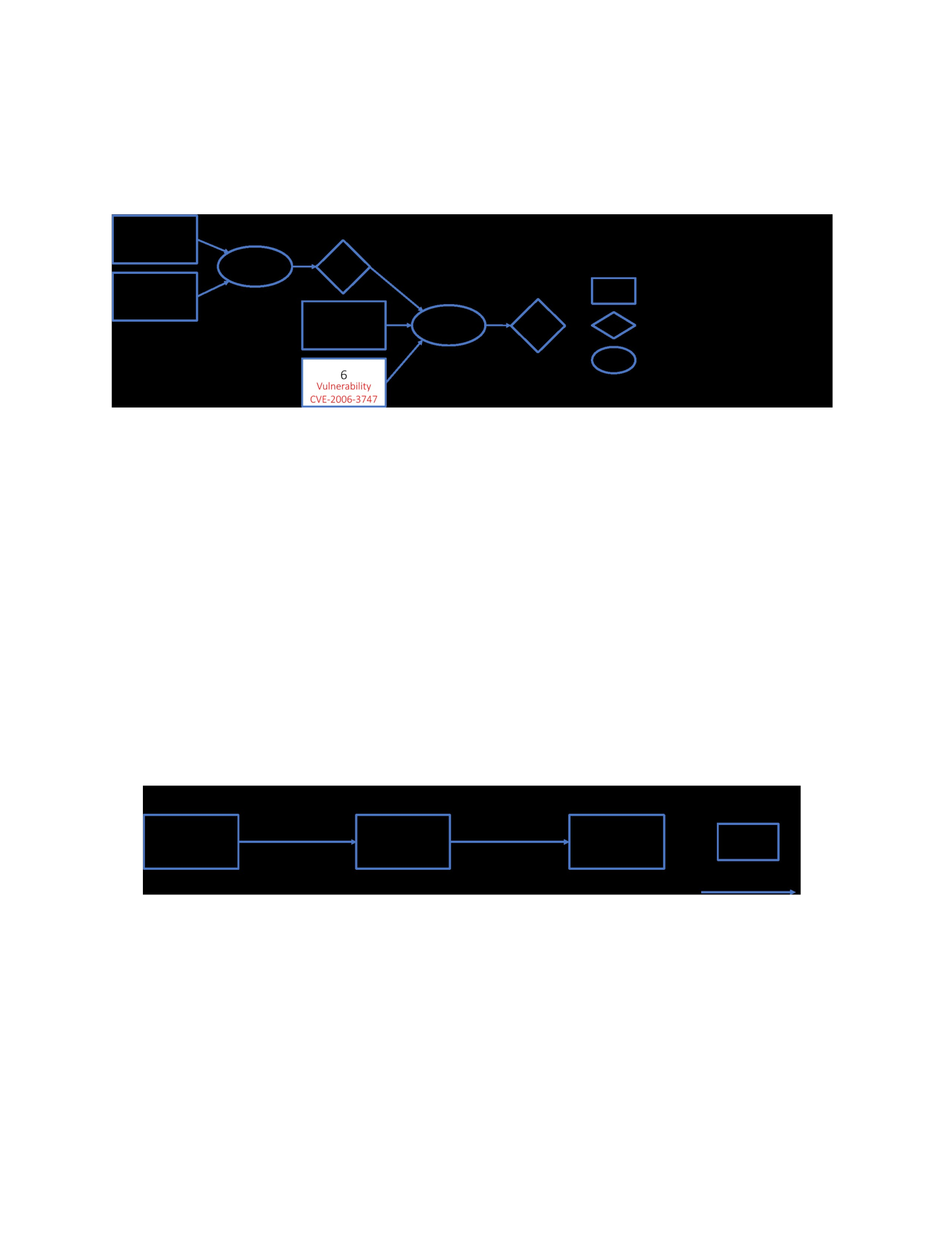
made by who generates the attack graph (Haque et al., 2017). Figures 2 and 3 present the same
attack sequence with different representation approaches. In Figure 2, rectangles represent the
system configurations, diamonds represent potential privileges an attacker could gain, and
ellipses represent the attack nodes. This is a very detailed way of visualizing an attack graph
where all prerequisite conditions of an attack can be seen easily. Each node has an identifier
number. Ellipse attack nodes have a probability of success value. The first step is to access the
web server from the internet, which has a probability of 1 since it is open to public access. The
second step is exploiting a vulnerability on the Apache web server to gain privileges of executing
arbitrary code on the web server (Tatar et al., 2020).
Figure 4.
23
Sample attack graph (Singhal & Ou, 2011)
It is typical that in attack graphs, nodes represent the states of network components, and
edges represent the transitions among different states. This formalism is less confusing than the
one in Figure 4 since it focuses on the steps of the attack with a smaller number of nodes. In our
study, this representation is employed since the increase in the number of ICT components leads
to very complicated graphs (Tatar et al., 2020).
Figure 5.
Different representation of the sample attack graph on Figure 4
Attack graphs are an evolved version of attack trees and fault trees. The purposes of using
each of these three approaches overlap in some manner. They all seem similar and are analyzed
using akin procedures. Differences arise in reading them and their application domains (e.g.,

24
military, energy systems, cybersecurity). Since some of the concepts used in the generation and
analysis of the attack trees were adopted from attack tree and fault tree approaches, these were
included in this report to help better understand (Tatar et al., 2020).
Similarities and Differences of Attack Graphs with Attack Trees and Fault Trees
Attack Trees are used for assessing ICT security. The difference between an attack graph
and an attack tree is what the edges and nodes represent. A complete attack tree looks like a tree
where the root is the eventual target, and the leaves are the elementary attacks (Haque et al.,
2017).
Attack trees provide a convenient visualization for comparing different attack strategies
on a specific target. Comparison factors can be changed to have a look at the security of the
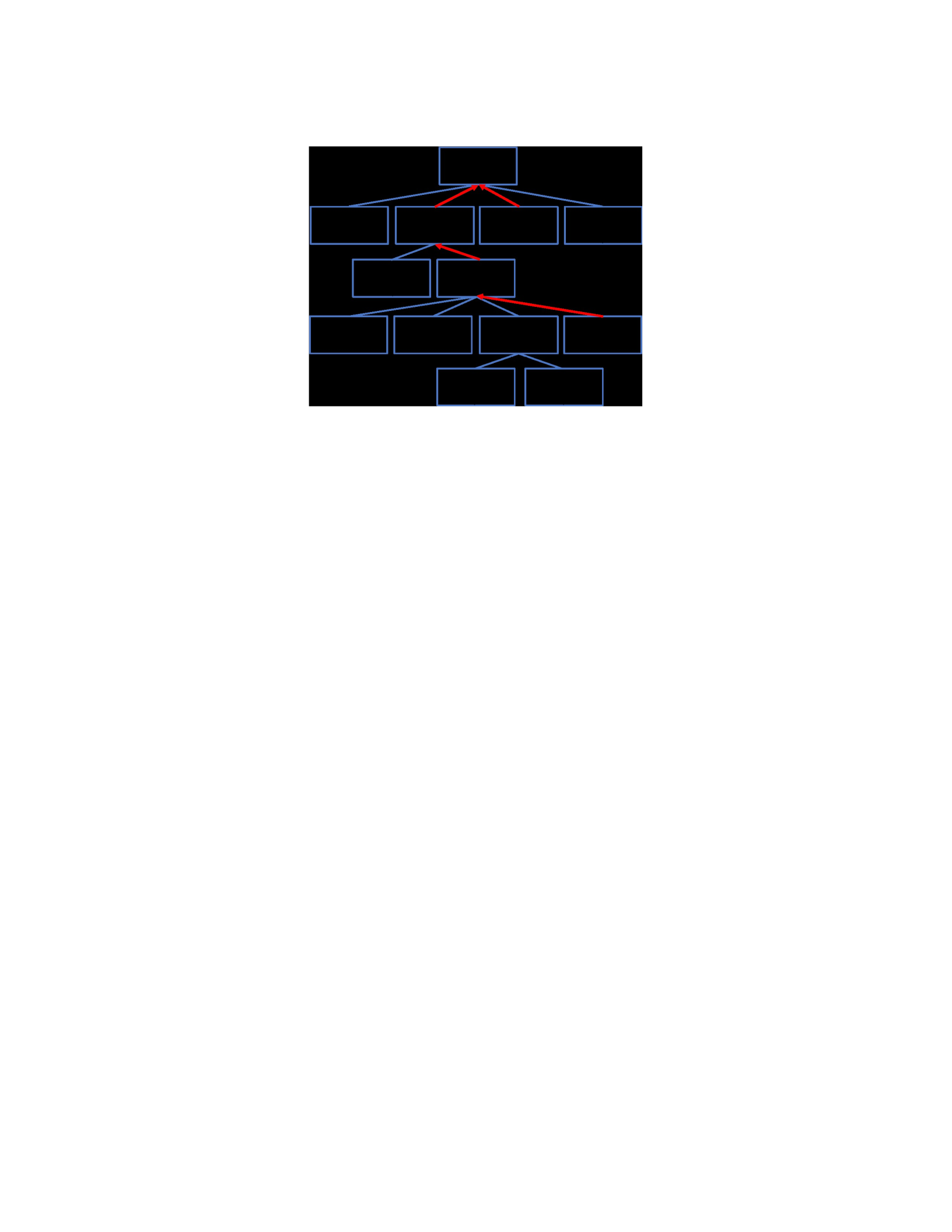
system from different perspectives. In a basic example of an attack tree against a safe box from
Schneiner (1999), it is seen that there are four main approaches to open the safe, and one of them
has multiple steps to be successful, as seen in Figure 6 (Tatar et al., 2020).
In Figure 6, the target is located at the top of the tree. This graph can be seen as an
upsidedown tree where the root is the target, and different strategies are the branches. Each of the
other boxes represents an attack phase. There are four main approaches, and three of the main
strategies are one-step attacks where “Learn Combo” has prerequisite attack steps (Tatar et al.,
2020).
Figure 6.
A simple attack tree example (Schneiner, 1999)
25
In order to analyze the attack to the safe from the attacker’s perspective, the four
approaches can be considered to see if they are possible or impossible to achieve for a certain
level of expertise of the attacker. Some of the steps are combined with AND logic, which means,
for example, to eavesdrop on the combo of the safe, the attacker must be able to both listen to the
conversation and get the target person to state the combo in a conversation. In this case, even if
listening is possible, getting the victim to state the combo is considered impossible, making the
eavesdropping approach impossible to open the safe. In this attack tree, all nodes are combined
with OR logic unless it is stated as an AND logic. In this example, only two approaches indicated
with red arrows are reasonably possible: cutting safe open and learning the combo from the target
person by bribing (Tatar et al., 2020).
Once an attack tree is ready for analysis, it can be taken into consideration from different
perspectives, such as whether it is possible for a particular type of malicious actor. Moreover,
other analyses can be conducted based on the estimated cost to the attacker, the requirement of
any special equipment, and the required time to complete. Security officials should consider the
26
system using the attack tree from various perspectives against the skills and resources of possible
adversaries (Tatar et al., 2020).
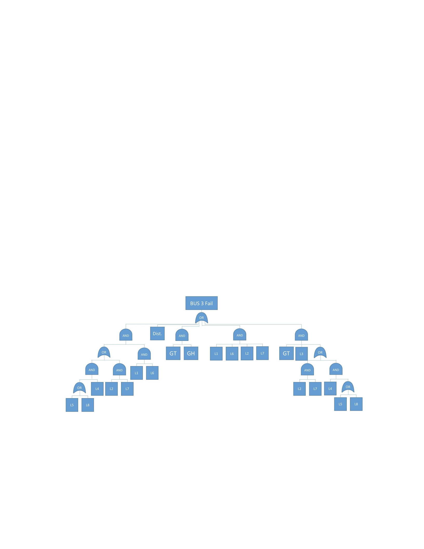
Fault Tree Analysis has been employed for decades to calculate the effects of component
failure and reliability of the systems such as military systems and power grids. Fault trees are
used to calculate how failure behavior, which is distributed randomly or based on a particular
probability distribution, changes the overall system’s reliability (Ingoldsby, 2010). Figure 7
presents an example fault tree where the reliability of the node at the top is analyzed using the
probabilities of failure of the square nodes, which are failure of specific components with a
failure rate with respect to a known probability distribution (Tatar et al., 2020).
Figure 7.
An example fault tree
Attack graphs are employed in this research. The details of the concepts that are used in
this study are explained in Chapter 4.

27
Modeling the Stepping Stone Attacks Using Attack Graphs
Attack graphs help model multi-step cyber-attacks that exploit various vulnerabilities that
exist in a sequence of hosts and workstations. This is a beneficial approach to assess the security
of well-protected cyber assets. It is expected that several paths exist on an attack graph for a
significant target. Nicol and Mallapura (2014) employed a deterministic approach to benchmark
the existing paths to find the shortest paths on these stepping stone attacks using attack graphs.
The weights of the edges are determined using some of the CVSS exploitability scores. The
shortest path is identified based on the total weights of the edges on the path to the target host.
This is a fundamental approach for identifying the paths. More advanced approaches employ
Bayesian Networks on the same problem of assessing stepping stone attacks.
Bayesian Attack Graph for Risk Analysis
Bayesian Networks are applied to attack graphs in order to assess network security by
calculating probabilities for each specific node on an ICT network (Singhal & Ou, 2011; Shetty,
2018; Shetty et al., 2018; Wang et al., 2008; Xie et al., 2010; Poolsappasit et al., 2012). Typically,
the probability of an exploit happening against a specific vulnerability is determined by using
publicly available CVSS metrics. Since these exploits are commonly chained after a preceding
exploit, the probability assigned in this manner is called conditional probability. By analyzing the
attack graph, the unconditional probability value for each node is computed by considering all
preceding probability values on all possible paths (Singhal & Ou, 2011; Shetty et al., 2018).
Wang et al. (2008) suggest an attack-graph-based probabilistic metric for network
security, adapting existing metrics like CVSS, which typically deal with individual
vulnerabilities. The authors integrate the measurements of individual vulnerabilities acquired

28
from existing metrics to determine an overall score of the network. The causal relationships
between vulnerabilities encoded in the attack graph enable the combination to perform. Another
novelty of their research is the approach to handle cycles that may naturally exist in attack
graphs. Without handling such cycles, calculations for Bayesian attack graphs can be difficult to
conduct. The new method addresses interdependencies on the network; however, still missing
monetary value and functionality of the nodes on the network.
Over time, some researchers employed the Common Vulnerability Scoring System
(CVSS) in attack graphs and attack trees. However, due to the nature of the CVSS, it takes into
account the vulnerability of an individual node in the network but not the effect of this
vulnerability on other nodes’ vulnerability level that can be exploited via the link of attacks
(Gallon & Bascou, 2011). Hence, attack graphs based on CVSS do not produce information on
the severity level of complex attacks. Though it has been proposed to use the CVSS framework
in attack graph to be able to compute the severity level of a complete attack scenario instead of
an attack targeting a single vulnerability, it still misses the monetary value of the risk and ripple
effects.
To better understand the causal dependencies between network states, Poolsappasit et al.
(2012) proposes a risk management model using Bayesian networks that enable a system
administrator to measure the likelihood of network compromise at different levels. The authors
call the method as Bayesian Attack Graphs, which adapts the idea of Bayesian belief networks.
The method helps to estimate an organization’s cyber risk from various vulnerability
exploitations. It also helps to measure the expected return on investment according to the
probability of system compromise and user-specified cost model. The paper benefits from CVSS

29
and addresses risk and causal relationships on a network. However, the functionality of the nodes
on a network might have a different level of dependency, and the proposed method does not
calculate it.
Another study on Bayesian attack graphs by Xie et al. (2010) focuses on the uncertainty
aspect. They suggest that uncertainty in cybersecurity studies has an important role. For example,
even if an initial security scan shows that vulnerabilities exist for exploitation, it does not mean
that they will be exploited for sure. Their model handles identifying and representing the
uncertainty relationships for the ITS systems.
Common Vulnerability Scoring System (CVSS)
Since CVSS is commonly employed in Bayesian attack graph studies, a short introduction
to CVSS is presented in this section of the literature review. Relevant technical specifications are
presented in chapter 3. CVSS is a vulnerability evaluation metric developed by FIRST.Org Inc.
(2019b) to communicate the severity of software vulnerabilities. It is used extensively in
vulnerability studies as a standard. The latest version is CVSS 3.1.
Basics of CVSS
CVSS is used by answering questions for each metric. According to the characteristics of
the vulnerability, it provides a score ranging from 0 to 10.
There are three main metric groups in CVSS: Base metrics, Temporal metrics, and
Environmental metrics. Base metrics are common for a vulnerability within all organizations and
are not affected by time. Base metrics include Attack Vector, Attack Complexity, Privileges
Required, and Impact Metrics for Confidentiality, Integrity, and Availability. Temporal metrics

30
can change in time, such as Exploit Code Maturity, Remediation Level, and Report Confidence.
Environmental metrics exist to adapt the score to each organization and include Security
Requirements and Modified Base Metrics (FIRST.Org Inc., 2019a).
Base metric values are required to be determined in order to be able to calculate the score.
Temporal and environmental metrics are optional. Users may apply any available information to
update the score according to additional information about the code’s exploit maturity or effects
on a specific organization (FIRST.Org Inc., 2019b).
National Vulnerability Database and Common Vulnerabilities and Exposures
National Vulnerability Database (NVD) (n.d.) provides all known hardware and software
vulnerabilities along with their CVSS scores. NVD is maintained by the National Institute of
Standards and Technology (NIST). Common Vulnerabilities and Exposures (CVE) are listed by
MITRE corporation and fed into NVD. Depending on the availability, the information provided
for each vulnerability includes a short description, affected software, CVSS 2.0 and CVSS 3.1
base scores, and information about any official patches or comments from the manufacturer or
developer (Tatar et al., 2020).
Assessing the Impact on the Business Processes
Impact on a business process of an enterprise can be calculated by knowing the services
and assets that make the business process possible. Jakobson (2011) presented a framework that
helps assess the impact on an enterprise's business processes, services, and assets. The framework
introduces the cyber terrain of an enterprise as a multilayered environment where assets
contribute to providing services, and services enable the business processes. The impact

31
dependency graph is presented to assess how the impact of a cyber-attack on some assets affects
the impact on specific business processes.
Deterministic and probabilistic approaches exist in the literature to assess the impact on
the business processes.
Deterministic Approaches
FDNA has been developed as a deterministic analysis tool (Garvey & Pinto, 2009). It
helps determine the effect of the inoperability of some components of the system on the
capabilities of the enterprise. Enterprise capability portfolio is considered a graph where
functional dependencies among the nodes are calculated to assess the impact propagation. This
approach helps reveal the cascading effects within the enterprise system components.
After the FDNA model of the enterprise has been developed, the decision-makers can
simply conduct deterministic analysis to test the organization's response against different
interruptions. The model enables performing what-if scenarios to assess the outcomes of the trials
(Guariniello & DeLaurentis, 2017).
In order to conduct deterministic analyses on enterprise ICT networks, the FDNA-Cyber
model has been developed (Tatar, 2019). This model adapts and applies the FDNA algebra to the
cyber domain by introducing concepts such as logic gates, self-efficiency, and confidentiality,
integrity, and availability components. With these improvements, the FDNA-Cyber model of an
enterprise can be used to perform what-if scenarios to test how a specific cyber incident affects
the assets of an enterprise and by dependency relations, how it affects the services, and
eventually what would be the impact on the business processes. Such scenario analyses help

32
decision-makers decide where to invest in cybersecurity products or other risk mitigation
strategies so that the overall cyber risk of the enterprise is decreased.
Probabilistic Approaches
Deterministic analysis can be time-consuming in simulating the model's inputs within
wide ranges instead of specified constant values. Adding probabilistic analysis capability to
FDNA enables decision-makers to understand the system’s behavior against multiple interruption
cases by generating probability density functions for the viability of the business processes
(Guariniello & DeLaurentis, 2017).
Sun et al. (2014) included a vulnerability layer to a three-layered impact assessment
model. They developed a probabilistic impact propagation approach in order to assess how the
existence of vulnerabilities on assets impacts the business processes. Probabilistic characteristics
of vulnerabilities are integrated within the model's calculations to assess better the impact on a
mission (i.e., a business process for businesses).
Another approach was developed by Sun et al. (2015) to assess the impact on the business
process by using a probabilistic bottom-up approach. The model considers the probability of the
intrusion propagation process, and impact propagation is calculated using the Bayesian network.
The probabilistic analysis could be conducted by giving all values in a range from 0 to
100 to self-efficiency of the nodes as input to the FDNA model. The outputs of such probabilistic
analysis can be the probability density function of operability values of the dependent nodes. This
approach can help understand the whole system's behavior as a function and gives more insights
into risks posed by the enterprise. To analyze the system’s behavior as a function, probabilistic
analysis capability for FDNA-Cyber was developed.

33
Temporal Effects
Regular risk quantification models only can assess the system as a snapshot rather than
allowing analysis over time. The temporal aspect of impact assessment helps decision-makers
evaluate the change of the system status over time and better estimate the impact.
For example, a multistage attack involving several exploitations and user interaction may
take a long time from start to success. Intrusion detection systems can detect suspicious activity
within the network. Even though the eventual target cannot be reached, some of the nodes have
already been affected. The ability to conduct temporal analysis can also help simulate such
scenarios for better-informed decision-making.
Sun et al. (2014) introduced the time factor to their multilayered impact evaluation model
for cyber-attacks targeting business processes. Their approach to include time is a categorical
variable called timeliness, referring to the time from the initialization of an attack to the
emergence of attack impact. They employed this variable as a component for the calculation of
the attack probability.
Other methods that allow temporal analysis includes Markov Process analysis (Xu &
Hua, 2017). This approach is employed for the systems with defined states and with probabilities
to change from one another among these states (Pinto & Garvey, 2012). This method is a
convenient way of analyzing the probabilistic state transition over time.
Integration of Attack Graph into Dependency Graph
Impact graphs assess the impact propagation among the layers of an enterprise; however,
an attack graph assesses the attack propagation among assets of an enterprise exploiting the

34
vulnerabilities within these assets. Integration of these two assessments benefits risk
quantification effort.
A model was developed by Sun et al. (2017) to interconnect the business process
dependency graph and cloud-level attack graphs. This helps find the impact caused by the
weakest links on the business processes. This study provides a graphical model to perform this
connection; however, it does not provide any quantitative algebra for the assessment.
Another study by Liu et al. (2017) develops a similar model but employs it in forensics
study after the event to understand what had happened. According to the evidence after the
incident, missing parts of the attack graph are reproduced using this model, and impact
assessment for business processes can be conducted.
A model that provides a numerical score for the impact on the business processes was
developed by Cao et al. (2018). The developed model aims to relate the impact on the business
processes as functions of CVSS scores of the vulnerabilities on the assets. They also present a set
of rules to prune the interconnected graphs to simplify the visual output graph.
There is progress on integrating attack graphs into dependency graphs; however, the
quantitative analysis does not go further than propagating the CVSS scores. The strength and
criticality of dependencies among the nodes of the impact graph is still a substantial gap to be
filled.
Functional Dependency Network Analysis (FDNA)
FDNA is a graph-based formalism to calculate the effects of interdependencies among
components of a system. It was developed by Garvey and Pinto (2009). It helps analyze impact
propagation when a component’s level of operability degrades for any reason. Functional

35
dependencies should be determined among the nodes of the system, and strength of dependency
and criticality of dependency parameters, which are the indicators of how crucial each
dependency connection is. More details about FDNA algebra are given in Chapter 3.
Previous Modifications and Applications of FDNA
FDNA was applied to a diverse set of fields and flexible for developing extensions to
adapt to the requirements of a specific problem.
Garvey et al. (2014) applied FDNA in a macro level study where industries become the
nodes of the enterprise. In this study, FDNA was integrated with the inoperability input-output
model, which is widely used in economics. This integration helps simulate what-if scenarios such
as the consequences of the electric power system of a metropolitan area failing.
Guariniello and DeLaurentis (2014a) apply FDNA to the cyber domain to quantify the
impact of cyber incidents so that comparing different architectures’ reliability and robustness
becomes possible. In another study, Guariniello and DeLaurentis (2014b) integrated functional
and developmental dependencies to analyze and compare properties of a system of systems by
applying them to a group of Navy entities. They introduced a new parameter, Impact of
Dependency, and provided probabilistic analyses in one of their succeeding study (Guariniello &
DeLaurentis, 2017).
FDNA was employed by Wang et al. (2014) to analyze the security impact of threats
against the Global Navigation Satellite System. This study conducted simulations to show the
validity of the method.

36
Another study employs FDNA (Costa et al., 2015) to simulate how the collapse of a bank
would affect the banking industry. They preferred removing one of the parameters, strength of
dependency, which does not fit the financial sector interdependencies well.
A probabilistic model was developed by adapting FDNA by Ozdemir et al. (2015). This
model assesses the technological development levels required to provide the capabilities required
of a long life cycle engineering product.
Another study applied FDNA into the cyber domain (Garrido-Pelaz et al., 2016) to
analyze information sharing among different organizations affected by various cyber-attacks. The
attack propagation is modeled by FDNA in this study, while information sharing decisions are
modeled by game theory.
A resiliency study by Servi and Garvey (2017) applied FDNA to develop new methods for
understanding an enterprise's response in overall rather than focusing on some specific nodes.
They also resented how the most critical nodes of the enterprise can be determined.
Short et al. (2018) adapted FDNA to develop a failure flow decision function
methodology where they could detect the critical components of the network to avoid any
possible failure.
Cole (2017) adapted FDNA to assess the data dependency among the nodes of a system of
systems. The model helps assess how data quality in one system affects the quality of data on
other systems within a system of systems. This study also includes an agent-based model of the
adapted model to help analyze and visualize the model.

37
CHAPTER 3
METHODOLOGY
Introduction
In this chapter, the methodology that was used to develop the model is explained. The
following sections recall the research question and objectives, summarize the phases of the
methodology, present the details about the relationship between the risk equation and attack
graphs, attack graph generation, CVSS, and impact graphs. These sections also provide details of
the previous studies that the developed model builds upon. The contributions made in this study
are explained in detail in the following chapter (Chapter 4).
Research Question and Objectives
Research Question: What probabilistic cyber risk analysis model can be developed by
considering cascading impacts through internal dependencies (e.g., vulnerabilities of assets to
business processes) and allowing temporal analysis?
In order to build a model that answers this question, four major research objectives should
be achieved.
Objective 1: Development of a customizable attack propagation model that adapts
vulnerability scoring by employing Bayesian attack graphs
Objective 2: Development of a probabilistic impact propagation assessment model by
considering dependencies and allowing temporal aspect
Objective 3: Development of a model integrating attack propagation and business impact
propagation to calculate economic impacts of cyber risks of an enterprise
Objective 4: Validation by simulation

38
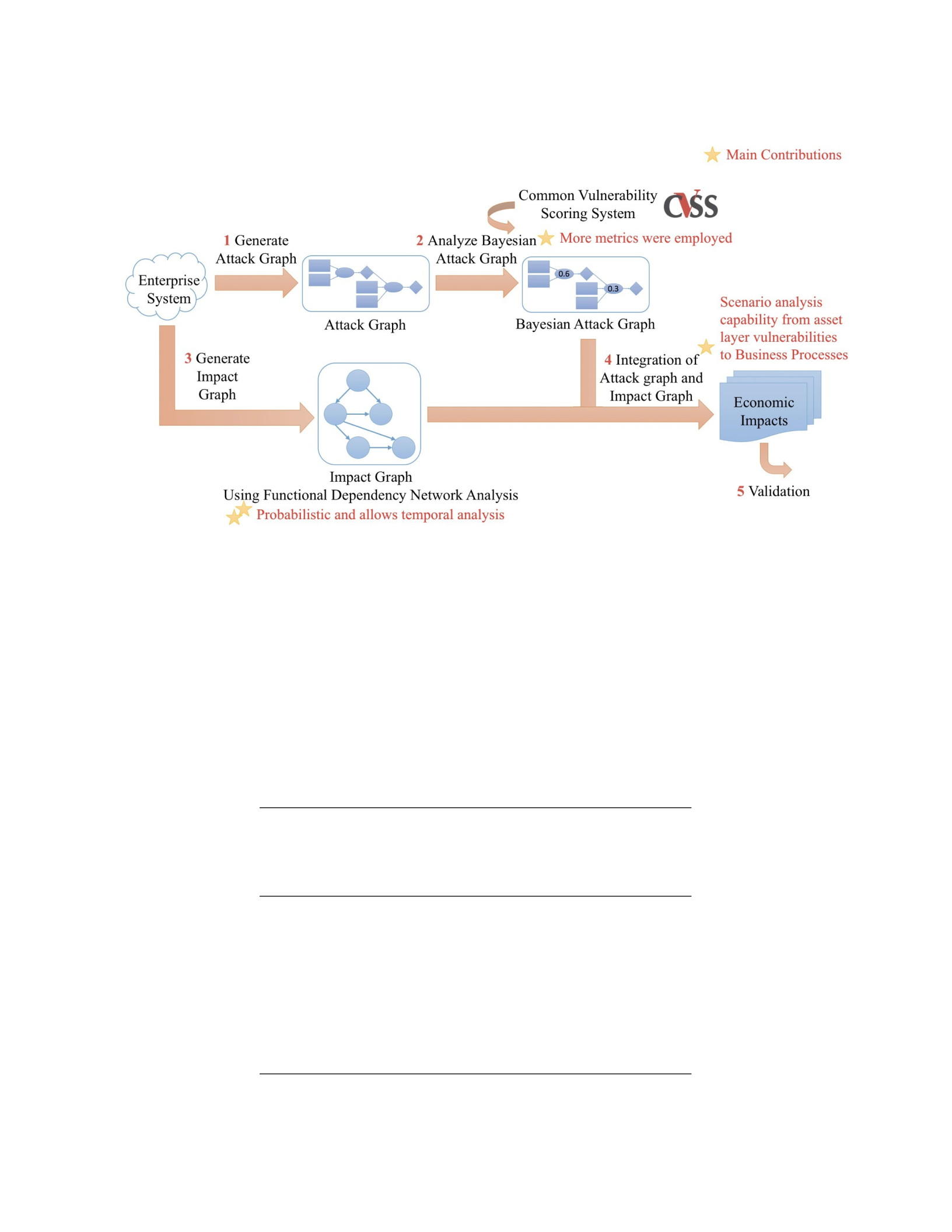
Phases of the Methodology
The phases of methodology to accomplish the research objectives are explained below
and illustrated in Figure 8:
1. Generate Attack Graph: Examine the enterprise ICT network vulnerabilities and
configurations of system and network to be able to generate the Attack Graph.
2. Analyze Bayesian Attack Graph: Establish and analyze the Bayesian attack graph by
considering likelihood and impact values of ICT vulnerabilities using CVSS
3. Generate Impact Graph: Generate and analyze the impact graph by employing Functional
Dependency Network Analysis for the Enterprise system by considering the assets,
services, business processes, and dependencies among them.
4. Integration of Attack graph and Impact Graph: Integrate the outputs of the attack graph of
the asset layer with the impact graph to assess the impact propagation within the impact
graph based on the outcomes of the attack graph.
5. Validation: Validate the developed methodology by developing a simulation model
investigating the economic impacts of enterprise business interruptions caused by
cyberattacks.
Figure 8.
Phases of the developed model
39
Mapping of the phases of the methodology with the research objectives is presented in
Table 2.
Table 2.
Mapping of the phases of the methodology with the research objectives
Phases of Methodology Research Objective
1 and 2 1
3 2
4 3
5 4

40
In the following three sections of this chapter, three major components of the method to
be developed are explained: generating attack trees, CVSS, and Impact graphs.
Risk equation and Attack Graph Relationship
Attack graphs help calculate the cyber risks of an organization. The risk is a function of
likelihood and impact (See Eq. 1).
𝑅𝑅𝑖𝑖𝑅𝑅𝑅𝑅 = 𝑓𝑓(𝑙𝑙𝑖𝑖𝑅𝑅𝑙𝑙𝑙𝑙𝑖𝑖ℎ𝑜𝑜𝑜𝑜𝑜𝑜, 𝑖𝑖𝑖𝑖𝑖𝑖𝑖𝑖𝑖𝑖𝑖𝑖) (Eq. 1)
•The likelihood of an attack depends on how experienced and motivated the
attacker is; therefore, likelihood is about the attacker.
•The impact depends on how critical the target network components are to the
organization; thus, the impact is about the victim.
The ease and benefits of conducting a cyber-attack are important factors in estimating the
likelihood of occurrence. Attack graphs, which examine networks from an attacker’s point of
view, are helpful to calculate the likelihood of a risk event (Ingoldsby, 2010). On the other hand,
the impact needs to be calculated based on how important the asset is and how it affects specific
services and business processes (Tatar et al., 2020).
This study uses Bayesian attack graphs to calculate the likelihood values and impact
graphs that employ Functional Dependency Network Analysis to compute the business impact
considering propagation.
Likelihood calculation using attack graphs requires detailed vulnerability information for
each asset on the attack graph. Detailed information is retrieved from the National Vulnerability

41
Database, where all known hardware and software vulnerabilities are presented using the
Common Vulnerability Scoring System.
Modeling and simulation of impact propagation is another aspect of this research. Impact
propagation depends on how each business process functionally depends on services and
individual assets within the enterprise ICT network. Functional Dependency Network Analysis is
a deterministic method to calculate the cascading effects of impact propagation among enterprise
layers (Tatar et al., 2020).
Attack Graph Generation
The inputs required for generating the attack graph for a network are (Swiler et al., 1998):
1. List of vulnerabilities within the network,
2. Network topology and specific network configurations, and
3. Database of known attacks.
There are numerous software packages for scanning a network to list all known
vulnerabilities that exist in the assets, such as computers, servers, routers, and software. Nessus
(n.d.) is one of the commonly used network vulnerability scanners. The output of a Nessus scan
and network topology is used to generate the attack graph by using software such as Topological
Analysis of Network Attack Vulnerability (TVA) (Jajodia et al., 2005), Network Security
Planning
Architecture (NETSPA) (Artz, 2002), and Multihost, multistage, Vulnerability Analysis
(MULVAL) (Ou et al., 2005; Tatar et al., 2020).
It is common for an enterprise to have many assets. Each of these assets may have
multiple vulnerabilities. With a large attack surface, an enterprise can have an attack graph with

42
so many attack paths. An attacker does not have every detail about an ICT network; therefore, it
would not be realistic to assume that an attacker would reveal all the attack paths a defender
could generate. The richness of an attack graph may lead a defender to conclude that the risk is so
high; however, the attack graph is a tool that helps find the critical nodes that are shared by
multiple attack paths.
Patching the vulnerabilities of such nodes would help mitigate the risks (Tatar et al., 2020).
Common Vulnerability Scoring System (CVSS)
CVSS is an identification, characterization, and assessment framework for Information
Technology vulnerabilities developed by the Forum of Incident Response and Security Teams
(Common Vulnerability Scoring System SIG, 2017). It is a publicly available framework.
CVSS has become a widely used vulnerability tool since its first release in 2004. It is
updated and improved regularly by adapting to changes in the information security environment.
It was adopted as Payment Card Industry Data Security Standard, and successfully passing the
CVSS became a security requirement for merchants using credit card payment systems. In 2007,
the National Institute of Standards and Technology (NIST) included CVSS in the Security
Content Automation Protocol. In 2011, CVSS was formally adopted as an international
vulnerability scoring standard (International Telecommunication Union, 2011).
In this study, the latest version is used, CVSS 3.1.
CVSS provides:
A standardization for Information Technology vulnerabilities,
An open framework helping users to understand the algorithm behind the tool,
Numeric scores to each vulnerability along with an explanation based on the
characteristics of the vulnerability,

43
Risk prioritization based on the score of each vulnerability and classifies them as critical,
high, medium, or low risk, and
A general assessment of the criticality of the complete IT system of the organization.
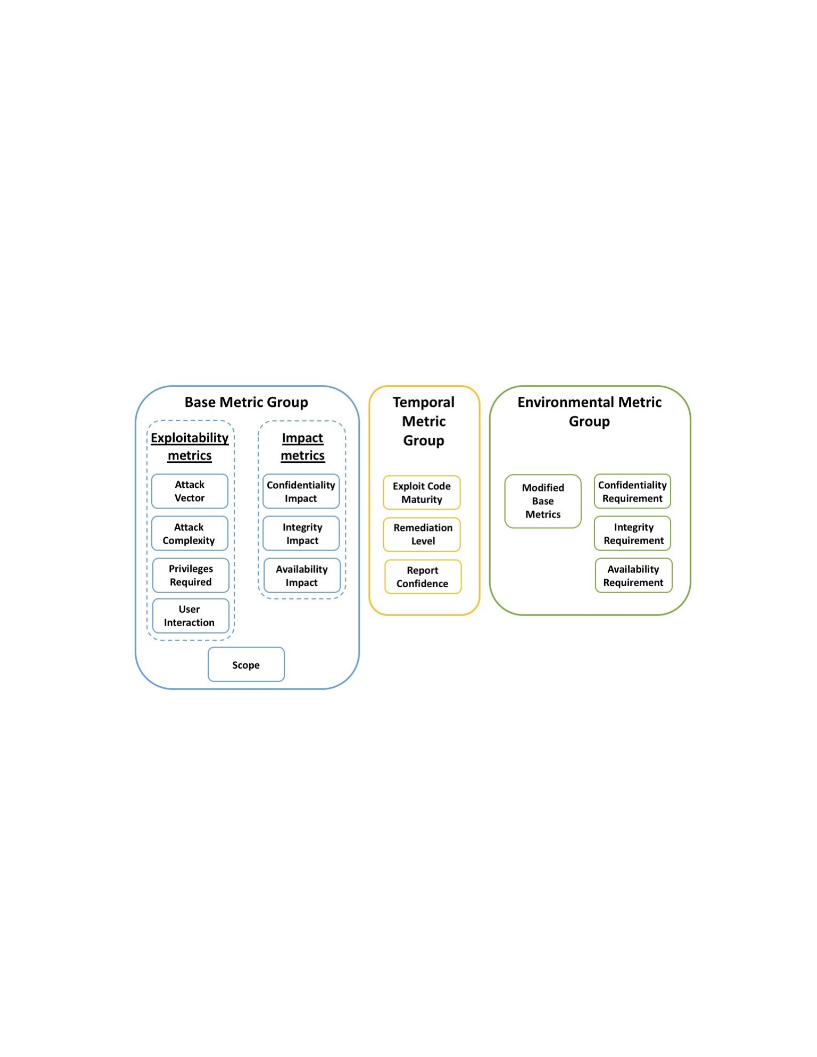
There are three metric groups of CVSS scores: base, temporal, and environmental metric
groups (Figure 9):
Figure 9.
Base Metric Group (Figure 10) calculates the intrinsic qualities of a vulnerability in two
sub-groups: exploitability and impact metrics. While exploitability metrics represent “the ease
and technical means by which the vulnerability can be exploited,” the Impact metrics represent
the consequences of that exploit on the confidentiality, integrity, and availability of the data and
services. Base metrics are Attack Vector, Attack Complexity, Privileges Required, and Impact
Metrics for Confidentiality, Integrity, and Availability.
Temporal Metric Group measures the current state of the maturity of exploit codes against
the vulnerability, the existence of any patches, or the confidence in the vulnerability’s
description. Temporal metrics are Exploit Code Maturity, Remediation Level, and Report
Confidence.
44
Environmental Metric Group helps assess the CVSS scores based on the environment of
the IT system concerning confidentiality, integrity, and availability requirements. Environmental
metrics are Security Requirements (Confidentiality Requirement, Integrity Requirement, and
Availability Requirement) and Modified Base Metrics (FIRST.Org Inc., 2019a).
Figure 10.
CVSS metrics of each metric group
The Base metrics generate a score from 0 to 10 that can be adjusted by rating the
Temporal and Environmental metrics. The CVSS database is updated regularly, and it reflects if
there are any developments about the vulnerabilities, such as patches.
Impact Graphs
In this study, for impact propagation analyses, Functional Dependency Network Analysis
(FDNA) is employed as the impact graph method. FDNA was developed to model and measure

45
dependency relationships between suppliers of technologies and providers of services these
technologies enable the enterprise to deliver (Garvey & Pinto, 2009; Tatar et al., 2020).
Summary of Functional Dependency Network Analysis
There are multiple aspects of the dependency problem in enterprise management. The
most important aspect is the analysis of cascading effects of failure in one function on the
operability of other dependent functions of the enterprise. FDNA provides a mechanism to
analyze these effects to minimize dependency risks that inherently exist in the system (Garvey &
Pinto, 2009).
The FDNA utilizes graph theory (Figure 11) to symbolize and model functional
dependency relationships between the nodes of the system. FDNA can be generalized as a
modeling and analysis tool for systems within a diverse set of fields, such as critical
infrastructure risk analysis, input-output economics, and dependency analysis problems (Garvey
& Pinto, 2009).
Figure 11.
An FDNA graph topology

46
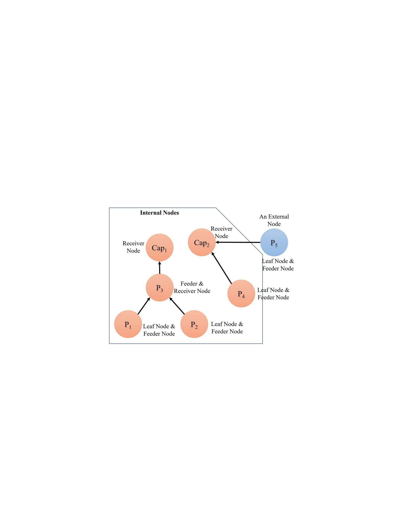
Baseline Operability Level (BOL) is the receiver node's operability level when its feeder
is entirely inoperable.
In FDNA, a receiver node’s operability level is affected by two dependency relations:
The first, Strength of Dependency (SOD) (0 < 𝛼𝛼𝑖𝑖𝑖𝑖 ≤ 1) is the strength with which a
receiver node’s operability level relies on the operability level of feeder nodes. SOD captures the
effects of relationships that increase the performance in addition to BOL.
The second, Criticality of Dependency (COD) (0 ≤ 𝛽𝛽𝑖𝑖𝑖𝑖 ≤ 100), is the criticality of
feeder node contributions to a receiver node for it to achieve its operability level objectives. COD
captures whether the dependency relationships could involve losses or constraints on these levels.
It governs how the performance of the receiver node will decrease below the BOL in time and
possibly become inoperable eventually.
Figure 12.
A 2-node FDNA graph
𝑃𝑃𝑖𝑖, which is the operability level of the receiver node 𝑁𝑁𝑖𝑖 in Figure 12, is dependent
on 𝑃𝑃𝑖𝑖, the operability level of its feeder node 𝑁𝑁𝑖𝑖, along with the two constraint of the
dependency between these two nodes: the strength of dependency and criticality of dependency.
Equation 2 shows the fundamental equation of the dependency:

47
𝑃𝑃𝑖𝑖 = 𝑓𝑓𝑃𝑃𝑖𝑖, 𝛼𝛼𝑖𝑖𝑖𝑖, 𝛽𝛽𝑖𝑖𝑖𝑖, 0 ≤ 𝑃𝑃𝑖𝑖, 𝑃𝑃𝑖𝑖 ≤ 100, 0 < 𝛼𝛼𝑖𝑖𝑖𝑖 ≤ 1, 0 ≤ 𝛽𝛽𝑖𝑖𝑖𝑖 ≤ 100
(Equation 2)
where 𝑗𝑗 depicts receiver (Child), 𝑖𝑖 depicts feeder (Parent), 𝑃𝑃𝑖𝑖 is operability level of the
receiver node, 𝑃𝑃𝑖𝑖 is operability level of the feeder node, 𝛼𝛼𝑖𝑖𝑖𝑖 is Strength of Dependency
(SOD) constraint, 𝛽𝛽𝑖𝑖𝑖𝑖is Criticality of Dependency (COD) constraint.
Based on FDNA’s original version (Garvey, 2009), the fundamental equation for the
operability level of node Py that is dependent on the operability levels of h other nodes, P1, P2, P3,
…, Ph, is defined as follows:
𝑃𝑃𝑦𝑦 = 𝑀𝑀𝑖𝑖𝑀𝑀 𝑆𝑆𝑆𝑆𝑆𝑆𝑃𝑃𝑖𝑖, 𝐶𝐶𝑆𝑆𝑆𝑆𝑃𝑃𝑖𝑖
0 ≤ 𝑃𝑃𝑦𝑦 ≤ 100
𝑆𝑆𝑆𝑆𝑆𝑆𝑃𝑃𝑖𝑖 = 𝐴𝐴𝐴𝐴𝑙𝑙𝐴𝐴𝑖𝑖𝐴𝐴𝑙𝑙 𝑆𝑆𝑆𝑆𝑆𝑆𝑃𝑃𝑖𝑖1, 𝑆𝑆𝑆𝑆𝑆𝑆𝑃𝑃𝑖𝑖2,
𝑆𝑆𝑆𝑆𝑆𝑆𝑃𝑃𝑖𝑖3, … , 𝑆𝑆𝑆𝑆𝑆𝑆𝑃𝑃ℎ
𝑆𝑆𝑆𝑆𝑆𝑆𝑃𝑃𝑖𝑖𝑖𝑖 = 𝛼𝛼𝑖𝑖𝑖𝑖𝑃𝑃𝑖𝑖 + 100 1 − 𝛼𝛼𝑖𝑖𝑖𝑖, 0 ≤ 𝑃𝑃𝑖𝑖, 𝑃𝑃𝑖𝑖 ≤ 100, 0 < 𝛼𝛼𝑖𝑖𝑖𝑖
≤ 1, 𝑖𝑖 = 1,2,3, … , ℎ
𝐶𝐶𝑆𝑆𝑆𝑆𝑃𝑃𝑖𝑖 = 𝑀𝑀𝑖𝑖𝑀𝑀 𝐶𝐶𝑆𝑆𝑆𝑆𝑃𝑃𝑖𝑖1, 𝐶𝐶𝑆𝑆𝑆𝑆𝑃𝑃𝑖𝑖2, 𝐶𝐶𝑆𝑆𝑆𝑆𝑃𝑃𝑖𝑖3, …
𝐶𝐶𝑆𝑆𝑆𝑆𝑃𝑃𝑖𝑖ℎ
𝐶𝐶𝑆𝑆𝑆𝑆𝑃𝑃𝑖𝑖𝑖𝑖 = 𝑃𝑃𝑖𝑖 + 𝛽𝛽𝑖𝑖𝑖𝑖, 0 ≤ 𝛽𝛽𝑖𝑖𝑖𝑖 ≤ 100 (1 − 𝛼𝛼𝑖𝑖𝑖𝑖)
Where SODPj: Strength of Dependency (SOD) equation of Pj on feeder nodes P1, P2, P3,
…, Ph
CODPj: Criticality of Dependency (COD) equation of Pj on feeder nodes P1, P2, P3,
…, Ph αij: Strength of dependency fraction of Pj on feeder nodes Pi
𝛽𝛽𝑖𝑖𝑖𝑖: Criticality of dependency fraction of Pj on feeder nodes Pi
48
FDNA helps to analyze the operability and business continuity of an enterprise by
considering possible ripple effects of any issue on the supplier functionality nodes. These issues
cause the inoperability of different capabilities of the enterprise. In Figure 13, the capability
portfolio of an enterprise is presented, including the external portfolio dependency node.
Figure 13.
An FDNA graph: a capability portfolio context (Garvey & Pinto, 2009)
In summary, FDNA is a methodology that enables decision-makers to analyze the
cascading effects of operability loss in a portfolio of feeder and receiver nodes. This ability
allows decision-makers to identify functionalities that are most critical to a portfolio's operational
capabilities (Garvey & Pinto, 2009).
Modified FDNA for Cybersecurity Application
FDNA-Cyber (Tatar, 2019) modified FDNA to quantify the cyber risks of enterprises. The
modifications include constituent nodes with confidentiality, integrity, and availability

49
components, self-efficiency of each node, AND and OR logic dependencies, and cost estimation
using the impact graph outputs (Tatar, 2019).
In this study, FDNA-Cyber was modified in two significant capabilities. The first
capability is to include probabilistic analysis to assess the inputs with stochastic behavior for
parameters such as the strength of dependency and the criticality of dependency. The second
capability to add to FDNA-Cyber is the temporal aspect. Temporal analysis helps assess the
status of the ICT system overtime under the effect of cyber incidents. How these modifications
were implemented is explained in Chapter 4.
The impact dependency graph in Figure 14 introduced a multi-layered dependency view
for an enterprise from a cyber network perspective (Tatar, 2019; Bahsi et al., 2018; Jakobson,
2011; Shameli-Sendi et al., 2016). This approach depicts the enterprises by assigning its entities
into three layers named: asset layer, service layer, and business process layer. This helps
determine the boundaries of the network, functional nodes of the network, either as assets,
services, or business processes, and functional dependencies among these nodes. This network is
named an impact graph in this methodology.
•Asset layer consists of tangible and intangible assets, such as hardware, software,
data/information, and people/users. (Tatar, 2019; Bahsi et al., 2018; Jakobson, 2011;
Shameli-Sendi et al., 2016).
•Service layer entities represent the aggregated functions collaboratively run by the assets
and enable tasks and business processes. Examples of service layer nodes can be email,
video conferencing, internet connection. (Tatar, 2019; Bahsi et al., 2018; Jakobson, 2011;
Shameli-Sendi et al., 2016).
50
•Business process layer consists of the main value-adding functions of the enterprise that
are enabled by assets and services (Bititci & Muir, 1998). It is represented as the mission
layer in military organizations. (Tatar, 2019; Bahsi et al., 2018; Jakobson, 2011;
ShameliSendi et al., 2016).
A vertical dependency is, for example, a dependency relation of a business process on
service, while horizontal dependency is among the same layer nodes, as illustrated in Figure 14.
(Tatar, 2019; Bahsi et al., 2018; Jakobson, 2011; Shameli-Sendi et al., 2016).
Figure 14.
Impact dependency graph (A: assets, S: services, T: tasks, and B: business processes) (Tatar, 2019)

51
CIA Constituent Nodes. Each node represents the confidentiality, integrity, and
availability of the functional entity they refer to. Confidentiality ensures that only the authorized
users can access a piece of information (McCallister et al., 2010). Integrity ensures that only the
authorized users can modify a piece of information (Stoneburner, 2001). Availability ensures the
authorized users can access the data and services whenever they need to (Ross et al., 2016).
Impact on each node is represented by deficiencies of any of these aspects for the affected entity.
Each node is a constituent node representing a linear additive sum of the single-dimensional
value function (SDVF) of confidentiality, integrity, and availability (CIA), as depicted in Figure
15 (Keeney & Raiffa, 1976; Tatar, 2019). For example, if a computer is shut down due to a power
outage, it means its availability value decreases to zero. If each of CIA has equal weight (i.e.,
importance), the operability of the node decreases to 66.67 utils from 100 utils.
Figure 15.
An FDNA-Cyber CIA constituent node (Tatar, 2019)
Formal representation of this concept for the operability a node consisting of Ci, Ii, and Ai
are denoted by SDVFs 𝑉𝑉𝐶𝐶𝑖𝑖𝑥𝑥𝐶𝐶𝑖𝑖, 𝑉𝑉𝐼𝐼𝑖𝑖𝑥𝑥𝐼𝐼𝑖𝑖, 𝑖𝑖𝑀𝑀𝑜𝑜 𝑉𝑉𝐴𝐴𝑖𝑖𝑥𝑥𝐴𝐴𝑖𝑖 . The
operability function of Pi is as
follows (Tatar, 2019).

52
𝑃𝑃𝑖𝑖 = 𝑤𝑤𝐶𝐶𝑖𝑖𝑉𝑉𝐶𝐶𝑖𝑖 + 𝑤𝑤𝐼𝐼𝑖𝑖𝑉𝑉𝐼𝐼𝑖𝑖 + 𝑤𝑤𝐴𝐴𝑖𝑖𝑉𝑉𝐴𝐴𝑖𝑖
(Eq. 3)
where
𝑤𝑤𝐶𝐶𝑖𝑖 + 𝑤𝑤𝐼𝐼𝑖𝑖 + 𝑤𝑤𝐴𝐴𝑖𝑖 = 1
𝑉𝑉𝐶𝐶𝑖𝑖 = 𝑉𝑉𝐶𝐶𝑖𝑖(𝑋𝑋𝐶𝐶𝑖𝑖), 𝑉𝑉𝐼𝐼𝑖𝑖 = 𝑉𝑉𝐼𝐼𝑖𝑖(𝑋𝑋𝐼𝐼𝑖𝑖), 𝑉𝑉𝐴𝐴𝑖𝑖 =
𝑉𝑉𝐴𝐴𝑖𝑖(𝑋𝑋𝐴𝐴𝑖𝑖)
0 ≤ 𝑉𝑉𝐶𝐶𝑖𝑖, 𝑉𝑉𝐼𝐼𝑖𝑖, 𝑉𝑉𝐴𝐴𝑖𝑖 ≤ 100
Self Efficiency. Self Efficiency in FDNA-Cyber allows each node to have a degraded
operability value caused by any intrinsic causes even if all its dependent nodes are fully
operational. For example, considering a network switch and computer relation, it is possible the
computer to fail due to an internal error or a cyber-attack though the network switch is fully
operational. Self-efficiency allows the computer’s operability level to decrease due to the failure.
FDNA equation with self-efficiency parameter for a 2-node graph (Figure 12) is given below
(Tatar, 2019).
𝑃𝑃𝑖𝑖 = 𝑆𝑆𝐸𝐸𝑖𝑖 ∗ (𝑀𝑀𝑖𝑖𝑀𝑀𝑆𝑆𝑆𝑆𝑆𝑆𝑃𝑃𝑖𝑖, 𝐶𝐶𝑆𝑆𝑆𝑆𝑃𝑃𝑖𝑖) = 𝑆𝑆𝐸𝐸𝑖𝑖 ∗
(𝑀𝑀𝑖𝑖𝑀𝑀𝛼𝛼𝑖𝑖𝑖𝑖𝑃𝑃𝑖𝑖 + 1001 −𝛼𝛼𝑖𝑖𝑖𝑖, 𝑃𝑃𝐼𝐼 + 𝛽𝛽𝑖𝑖𝑖𝑖)
where SEj is self-efficiency of Pj and 0 ≤ 𝑆𝑆𝐸𝐸 ≤ 1
AND And OR Gate Dependency. FDNA-Cyber introduced AND and OR gate logic to
FDNA since, in certain conditions, the dependency of nodes can be represented by these gates’
logic. If a node requires the operability of both of its dependent nodes simultaneously, it is
represented by an AND gate. If the system has redundancy with replica assets, then the
dependency can be represented by an OR gate (Tatar, 2019).

53
Equations for a receiver node with two feeder nodes in three types of dependencies are
given below:
FDNA dependency:
𝑃𝑃𝑖𝑖 = 𝑆𝑆𝐸𝐸𝑖𝑖 ∗ 𝑀𝑀𝑖𝑖𝑀𝑀𝐴𝐴𝐴𝐴𝑙𝑙𝑆𝑆𝑆𝑆𝑆𝑆𝑉𝑉𝑖𝑖𝑖𝑖1, 𝑆𝑆𝑆𝑆𝑆𝑆𝑉𝑉𝑖𝑖𝑖𝑖2,
𝐶𝐶𝑆𝑆𝑆𝑆𝑉𝑉𝑖𝑖𝑖𝑖1, 𝐶𝐶𝑆𝑆𝑆𝑆𝑉𝑉𝑖𝑖𝑖𝑖2
AND gate dependency
𝑃𝑃𝑖𝑖 = 𝑆𝑆𝐸𝐸𝑖𝑖 ∗ 𝑀𝑀𝑖𝑖𝑀𝑀𝑀𝑀𝑖𝑖𝑀𝑀𝑆𝑆𝑆𝑆𝑆𝑆𝑃𝑃𝑖𝑖𝑖𝑖1, 𝐶𝐶𝑆𝑆𝑆𝑆𝑃𝑃𝑖𝑖𝑖𝑖1,
𝑀𝑀𝑖𝑖𝑀𝑀𝑆𝑆𝑆𝑆𝑆𝑆𝑃𝑃𝑖𝑖𝑖𝑖2, 𝐶𝐶𝑆𝑆𝑆𝑆𝑃𝑃𝑖𝑖𝑖𝑖2
OR gate dependency
𝑃𝑃𝑖𝑖 = 𝑆𝑆𝐸𝐸𝑖𝑖 ∗ 𝑀𝑀𝑖𝑖𝑥𝑥𝑀𝑀𝑖𝑖𝑀𝑀𝑆𝑆𝑆𝑆𝑆𝑆𝑃𝑃𝑖𝑖𝑖𝑖1, 𝐶𝐶𝑆𝑆𝑆𝑆𝑃𝑃𝑖𝑖𝑖𝑖1,
𝑀𝑀𝑖𝑖𝑀𝑀𝑆𝑆𝑆𝑆𝑆𝑆𝑃𝑃𝑖𝑖𝑖𝑖2, 𝐶𝐶𝑆𝑆𝑆𝑆𝑃𝑃𝑖𝑖𝑖𝑖2
Calculating Loss of Impact. FDNA-Cyber computes the economic impact by
interpolating the estimated costs for each cost factor based on the loss of operability of CIA
values for each business process. Cost estimate depends on the previous studies of the Council of
Economic Advisors (2018), Federal Bureau of Investigation (2017), Verizon (2017), and the
Open Web Application Security Project, where 13 cost factors of an adverse cyber event are
identified as: “(1) Loss of IP, (2) Loss of strategic information, (3) Reputational damage, (4)
Increased cost of capital, (5) Cybersecurity improvements, (6) Loss of data and equipment, (7)
Loss of revenue, (8) Public relations, (9) Regulatory penalties, (10) Customer protection, (11)
Breach notification,
(12) Court settlement fees, and (13) Forensics” (Table 3) (Tatar, 2019).

54
For example, when a distributed denial of service (DDoS) attack ceases operations of a
business. Then cost estimates for the availability-related cost factors (cost items) of the affected
business processes are used to compute the total estimated cost of the attack (Tatar, 2019).
Table 3.
Relation of potential consequences and cost factors (confidentiality, integrity, and availability) (Tatar,
2019)
Cost Factors
Cost Parameter Cost/Loss Item Confidentiality Integrity Availability
Ct1 Loss of IP X
Ct2 Loss of Strategic Information X X X
Ct3 Reputational Damage X X X
Ct4 Increased Cost of Capital X
Ct5 Cybersecurity Improvements X X X
Ct6 Loss of Data and Equipment X X X
Ct7 Loss of Revenue X X X
Ct8 PR X X X
Ct9 Regulatory Penalties X X X
Ct10 Customer Protection X
Ct11 Breach Notifications X
Ct12 Court Settlement Fees X X X
Ct13 Forensics X X X

55
The table is populated with the cost estimate for each business process by expert
elicitation. The time and duration of the attack are also important parameters of cost calculation.
The economic cost calculation formulas are given below (Tatar, 2019).
𝐶𝐶𝑜𝑜𝑅𝑅𝑖𝑖 (𝐵𝐵1) = 𝑓𝑓(𝐶𝐶𝐵𝐵𝐵𝐵1, 𝑖𝑖, 𝑜𝑜, 𝐼𝐼𝐵𝐵𝐵𝐵1, 𝑖𝑖, 𝑜𝑜, 𝐴𝐴𝐵𝐵𝐵𝐵1, 𝑖𝑖, 𝑜𝑜)
𝐶𝐶𝐵𝐵1 = 𝐴𝐴(𝐶𝐶𝑖𝑖1, 𝐶𝐶𝑖𝑖2, 𝐶𝐶𝑖𝑖3, 𝐶𝐶𝑖𝑖4, 𝐶𝐶𝑖𝑖5, 𝐶𝐶𝑖𝑖6, 𝐶𝐶𝑖𝑖7, 𝐶𝐶𝑖𝑖8, 𝐶𝐶𝑖𝑖9,
𝐶𝐶𝑖𝑖10, 𝐶𝐶𝑖𝑖11, 𝐶𝐶𝑖𝑖12, 𝐶𝐶𝑖𝑖13)
𝐼𝐼𝐵𝐵1 = 𝐴𝐴(𝐶𝐶𝑖𝑖2, 𝐶𝐶𝑖𝑖3, 𝐶𝐶𝑖𝑖5, 𝐶𝐶𝑖𝑖6, 𝐶𝐶𝑖𝑖7, 𝐶𝐶𝑖𝑖8, 𝐶𝐶𝑖𝑖9, 𝐶𝐶𝑖𝑖12, 𝐶𝐶𝑖𝑖13)
𝐴𝐴𝐵𝐵1 = 𝐴𝐴(𝐶𝐶𝑖𝑖2, 𝐶𝐶𝑖𝑖3, 𝐶𝐶𝑖𝑖5, 𝐶𝐶𝑖𝑖6, 𝐶𝐶𝑖𝑖7, 𝐶𝐶𝑖𝑖8, 𝐶𝐶𝑖𝑖9, 𝐶𝐶𝑖𝑖12, 𝐶𝐶𝑖𝑖13)
𝑛𝑛
𝑇𝑇𝑆𝑆𝑇𝑇𝐴𝐴𝑇𝑇 𝐶𝐶𝑆𝑆𝑆𝑆𝑇𝑇 = 𝐶𝐶𝑜𝑜𝑅𝑅𝑖𝑖(𝐵𝐵𝑘𝑘)
𝑘𝑘=1
Where B1 is a business process,
𝐶𝐶𝐵𝐵1is the cost of loss of confidentiality for B1,
𝐼𝐼𝐵𝐵1is the cost of loss of integrity for B1,
𝐴𝐴𝐵𝐵1is the cost of loss of availability for B1, t is the
time when the impact of cyber action is observed,
d is the duration of cyber action.
CHAPTER 4
MODEL DEVELOPMENT
Introduction

56
In this chapter, details of the developed model are presented. In this chapter, the
contributions of the study are explained in detail. The model presented in this chapter was
developed for the projects funded by the Society of Actuaries and the National Science
Foundation. Some parts of this dissertation were presented in the technical report of the Society
of Actuaries, entitled “Quantification of Cyber Risk for Actuaries” (Tatar et al., 2020), and
included in this dissertation with their permission.
The information in this chapter builds upon the foundations of the previous studies
explained in Chapter 3. The application of the developed model is covered in Chapters 5 and 6;
therefore, this chapter only provides the details of the model but not the practical examples on
how to use the developed model.
The following sections provide the details of Bayesian Attack Graphs and CVSS
integration, present how the impact graph is improved to conduct probabilistic and time-
dependent analyses, deliver the details on how to integrate attack graph and impact graph, and
present the details on cost calculation.
Enhanced CVSS Integration into Bayesian Attack Graphs
Models in the literature commonly use the outdated CVSS version 2. This study adapts to
changes in CVSS version 3.1. In this section, the metrics in version 3.1 are presented along with
which metric to be used in which part of the analyses. Then, the Bayesian Attack Graphs are
explained, and the steps to calculate conditional and unconditional probability values for each
node are presented.

57
CVSS Version 3.1 Metrics
The value of each metric is determined by answering a question about the characteristics
of the vulnerability. Questions and possible answers for Base Metrics are visualized in Figure 16.
Each possible metric value is also represented by a numerical value. For example, the Attack
Vector metric represents where the attacker is needed to be in order to be able to exploit the
vulnerability. In this case, there are four possibilities in the answer: Network, Adjacent, Local,
and Physical. If it is Network, it means that an attacker on the internet can exploit it. On the other
hand, if it is Physical, only an attacker who can physically touch and control the computer with
the vulnerability can exploit it, i.e., more challenging to exploit.
Figure 16.
CVSS base metric group questions and possible values

58
Temporal metrics are composed of Exploit Code Maturity (i.e., is exploit code available),
Remediation Level (i.e., is there a fix for this vulnerability), and Report Confidence (i.e., how
reliable is the source of the report). The valuation of these factors is explained in Figure 17.
Figure 17.
CVSS temporal metric group questions and possible values
Environmental metrics are composed of two sub-groups:
•Modified Base Metrics (to customize any of the metrics), and
•Confidentiality/Integrity/Availability Requirements (how vital they are for the asset).
The descriptions of environmental metrics are provided in Figure 18.
Figure 18.

59
CVSS environmental metric group questions and possible values
CVSS value of a vulnerability is represented as a Vector String, consisting of all the
information on the vulnerability in an abbreviated form. The abbreviations for each metric and
the possible values are presented in Table 4. An example of the vector string of an example
vulnerability, CVE-2019-10098 (National Vulnerability Database, 2019a), is shown below:
CVSS:3.1/AV:N/AC:L/PR:N/UI:R/S:C/C:L/I:L/A:N
The interpretation of the example vector string:
•CVSS Version 3.1
•Attack Vector: Network
•Attack Complexity: Low
•Privileges Required: None
•User Interaction: Required
•Scope: Changed

60
•Confidentiality: Low
•Integrity: Low
•Availability: None

63
Table 4.
Metric names, abbreviations, and possible values with abbreviations. Adapted from FIRST.Org Inc. (2019a)
Metric Group Metric Name (Abbreviation) Possible Values
Base Metric
Group
Attack Vector (AV)
Attack Complexity (AC)
Privileges Required (PR)
User Interaction (UI)
Scope (S)
Network (N), Adjacent (A), Local (L), Physical (P)
Low (L), High (H)
None (N), Low (L), High (H)
None (N), Required (R)
Unchanged (U), Changed (C)
Confidentiality (C) High (H), Low (L), None (N)
Integrity (I) High (H), Low (L), None (N)
Availability (A) High (H), Low (L), None (N)
Temporal
Metric Group
Exploit Code Maturity (E)
Remediation Level (RL)
Not Defined (X), High (H), Functional (F), Proof of Concept (P),
Unproven (U)
Not Defined (X), Unavailable (U), Workaround (W), Temporary Fix (T),
Official Fix (O)

Report Confidence (RC) Not Defined (X), Confirmed (C), Reasonable (R), Unknown (U)
64
Table 4. continued.
Metric Group Metric Name (Abbreviation) Possible Values
Environmental
Metric Group
Confidentiality Requirement (CR)
Integrity Requirement (IR)
Availability Requirement (AR)
Modified Attack Vector (MAV)
Modified Attack Complexity (MAC)
Modified Privileges Required (MPR)
Not Defined (X), High (H), Medium (M), Low (L)
Not Defined (X), High (H), Medium (M), Low (L)
Not Defined (X), High (H), Medium (M), Low (L)
Not Defined (X), Network (N), Adjacent (A), Local (L), Physical (P)
Not Defined (X), Low (L), High (H)
Not Defined (X), None (N), Low (L), High (H)
Modified User Interaction (MUI) Not Defined (X), None (N), Required (R)
Modified Scope (MS) Not Defined (X), Unchanged (U), Changed (C)
Modified Confidentiality (MC) Not Defined (X), High (H), Low (L), None (N)
Modified Integrity (MI) Not Defined (X), High (H), Low (L), None (N)
Modified Availability (MA) Not Defined (X), High (H), Low (L), None (N)

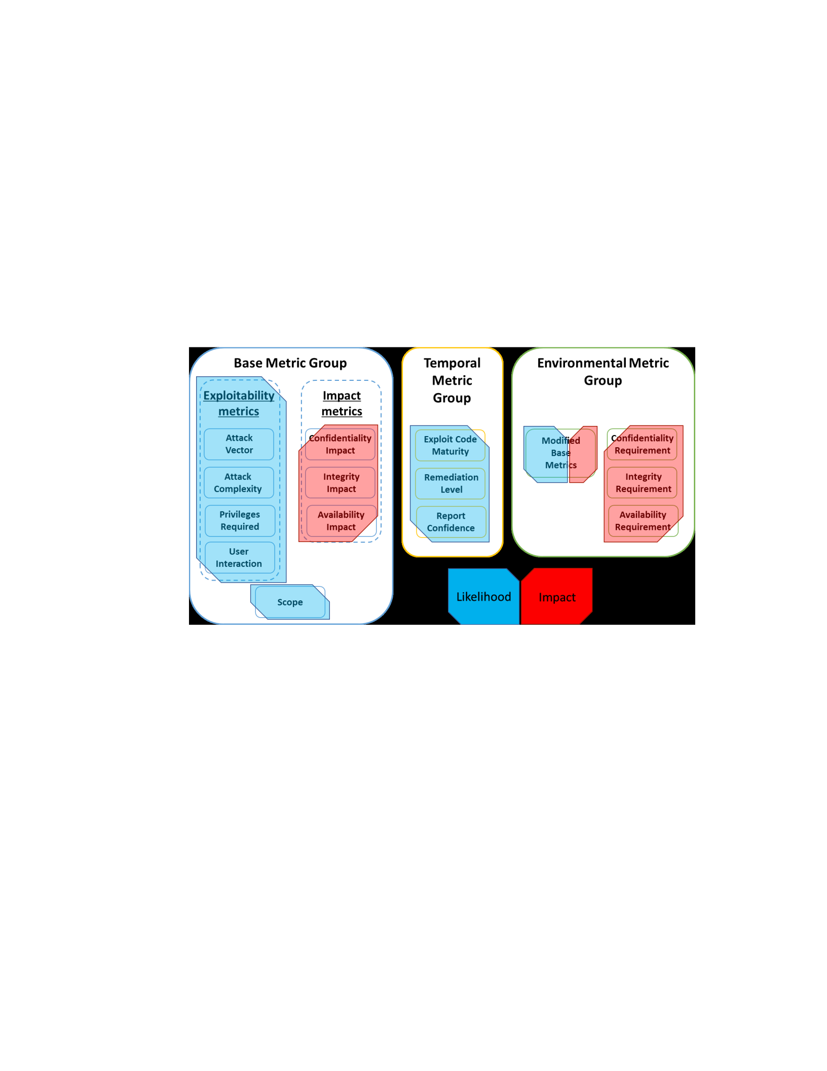
64
CVSS Metrics Included in the Model
In Figure 19, the CVSS metrics used for likelihood and impact calculations are highlighted
with cyan and red shapes, respectively.
Figure 19.
Metrics used for calculating likelihood and impact value
•Likelihood estimation is based on the Exploitability Metrics (Attack Vector, Attack
Complexity, Privileges Required, and User Interaction), Scope, Temporal Metrics
(Exploit Code Maturity, Remediation Level, and Report Confidence), Modified
Exploitability metrics (Modified Attack Vector, Modified Attack Complexity,
Modified Privileges Required, and Modified User Interaction), and Modified Scope
(See Figure 19).
•Impact estimation is based on Impact Metrics (Confidentiality Impact, Integrity

65
Impact, and Availability Impact), Modified Impact Metrics (Modified
Confidentiality Impact, Modified Integrity Impact, and Modified Availability
Impact), and Security Requirements (Confidentiality Requirement, Integrity
Requirement, and Availability Requirement) (See Figure 19).
Temporal and Environmental metrics can be used within the developed model; however,
these are optional and are not provided in National Vulnerability Database (NVD). The values
are required to be manually determined and applied to the calculations. The Base and Temporal
metric values for a vulnerability are specified by vulnerability analysts, security product vendors,
or application vendors as being knowledgeable about the characteristics of a vulnerability in a
system. On the other hand, the end-user organizations must specify the environmental metrics
since they know their computing environment better than anyone else and can anticipate the
potential impact a vulnerability can cause (FIRST.Org Inc., 2019a).
Bayesian Attack Graph for Risk Analysis
Based on the number and characteristics of the vulnerabilities of an ICT asset, a
likelihood of attack can be calculated. However, in multi-step attacks in which the attacker
exploits a vulnerable system to use as a stepping stone for the actual target, using the individual
likelihood values coming from each vulnerability would be insufficient to calculate the overall
cyber risk of the network. In order to calculate the likelihood of a multi-step attack, individual
probabilities need to be combined. Such cumulative probabilities are computed employing
Bayesian Networks on attack graphs which introduces the concepts of Bayesian Attack Graphs.
For example, Figure 20 represents an attack graph where the hosts (ICT network components)
are indicated as nodes. A, B, and C are hosts within the system, and D is the attacker on the internet.
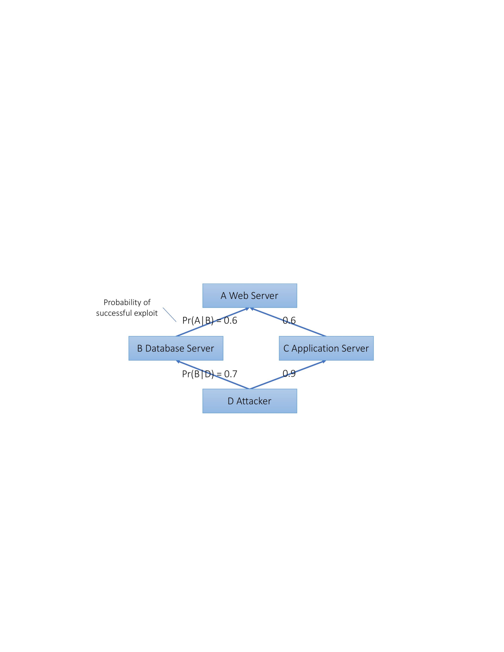
66
The attacker can use either the database server or application server to reach the target, the web
server. The conditional probabilities of exploitation are indicated on the edges just before each host
that has the vulnerability. The probability of a vulnerability in the database server being successfully
exploited given that the attacker wants and is capable of exploiting is 0.7 and notated as Pr(B|D). This
probability value is estimated according to the intrinsic characteristics of the vulnerability that exists
in the database server.
Figure 20.
Sample Bayesian attack graph (Poolsappasit et al., 2012)
There are two attack paths on this attack graph. Either way would suffice the attacker to
hack into the web server. The two paths are connected with an OR logic to the web server and are
not prerequisites of one another.
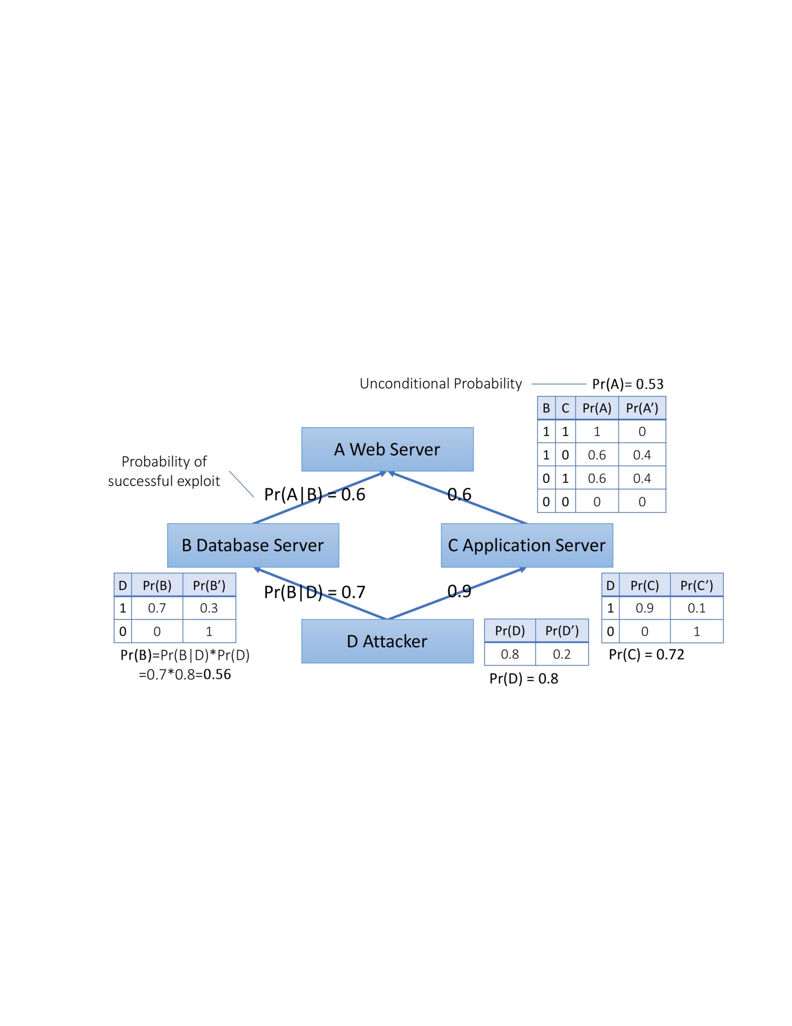
67
Calculating Local Conditional and Unconditional Probabilities. Bayesian logic is
used to analyze the attack graph as a whole and provide unconditional probabilities for each node
by considering all predecessor probabilities. In Figure 21, the details of an unconditional
probability calculation of the Bayesian attack graph are given.
Figure 21.
Probabilities of Bayesian attack graph nodes (Poolsappasit et al., 2012)
First, a probability is assigned based on the defender’s experience to the attacker to start
an attack on the network. Pr(D) = Pr (D = True) is assigned 0.8 in this case. Pr(D’) = Pr (D =
False) is the probability that the attacker would not attack and calculated by subtracting Pr(D)
from 1.
Some of the following calculations build upon Pr(D) probability value as chains. The tables within

68
Figure 21 represent a local conditional probability distribution function. These tables only include
local probabilities (i.e., the host with the vulnerability and the condition of the previous nodes).
The tables show all possibilities for local conditions and provide the probabilities. For example,
as shown in Table 5, the probability of successfully exploiting a vulnerability in the application
server is 0.9, given that the attacker is willing and capable to attack. In this case, Pr(C|D) is equal
to 0.9; (this can also be notated as Pr(C|D=True) = 0.9). The probability of not exploiting the
vulnerability given that the attacker is willing and capable of attack is Pr(C’|D) = 1- Pr(C|D) =
0.1. Since this exploit cannot be successful without the attacker's intention, its probability is zero;
thus, Pr(C|D’) = 0.
Table 5.
Local conditional probability distribution for C (i.e., application server)
D Pr(C) Pr(C’)
1/True Pr(C|D) = Pr(C|D = True) = 0.9 Pr(C’|D) = Pr(C’|D = True) = 0.1
0/False Pr(C|D’) = Pr(C|D = False) = 0 Pr(C’|D’) = Pr(C’|D = False) = 1
Calculating the local conditional probability distribution for the nodes with OR logic,
probabilities of all paths should be taken into consideration. The calculations are the same for the
other cases, with the only exception is when both nodes’ values are True. In the case that both
two predecessor nodes are already successfully exploited, the probability with the higher value
becomes the value for this node.
In order to understand the actual likelihood of a host to be exploited, the local conditional
probability distributions are not enough. The unconditional probabilities should be calculated by

69
considering all the previous events’ probabilities (Wang et al., 2008; Shetty et al., 2018; Hasan et
al., 2019a; Hasan et al., 2019b). For example, the probability of successfully exploiting the
vulnerability in the database server is 0.7, given that the attacker is willing to start the attack. The
probability of the existence of an attacker’s action is 0.8. Therefore, the unconditional probability
of the database server is exploited is calculated as follows:
𝑃𝑃𝐴𝐴(𝐵𝐵) = 𝑃𝑃𝐴𝐴(𝐵𝐵|𝑆𝑆) ∗ 𝑃𝑃𝐴𝐴(𝑆𝑆) = 0.7 ∗ 0.8 = 0.56
Similarly, the unconditional probability of successful exploitation of the vulnerability in the
application server is calculated as follows:
𝑃𝑃𝐴𝐴(𝐶𝐶) = 𝑃𝑃𝐴𝐴(𝐶𝐶|𝑆𝑆) ∗ 𝑃𝑃𝐴𝐴(𝑆𝑆) = 0.9 ∗ 0.8 = 0.72
As can be observed, even though conditional probability values are relatively high, the
unconditional probabilities are lower because of the nature of multi-step attacks. As the chain
gets longer, the likelihood of an attack to happen decreases significantly.
Finally, the unconditional probability of successfully exploiting the vulnerability in the
web server, which is the eventual target, is calculated by considering both attack paths. The OR
logic connection is made (Wang et al., 2008) as follows:
𝑃𝑃𝐴𝐴(𝐴𝐴) = 𝑃𝑃𝐴𝐴(𝐴𝐴|𝐵𝐵) ∗ (𝑃𝑃𝐴𝐴(𝐵𝐵) + 𝑃𝑃𝐴𝐴(𝐶𝐶) − Pr(𝐵𝐵) ∗ Pr (𝐶𝐶)) =
0.6 ∗ (0.56 + 0.72 − 0.56 ∗ 0.72)
= 0.53
The unconditional probability values are important metrics for calculating the risks posed by
each component of the ICT network. These calculations are extensively used in this study.
Probability Values of Successful Exploitation of Each Vulnerability (Likelihood).
Calculations of the local conditional probability distribution and unconditional probabilities are
explained above. These calculations depend on the probability values of the successful

70
exploitation of each vulnerability. This is also referred to as likelihood in this study. The
likelihood values are computed using specific metrics of CVSS base and temporal metric groups.
CVSS metrics provide information about likelihood and impact. The metrics relevant to
likelihood are as follows:
•Attack Vector (AV)
•Attack Complexity (AC)
•Privileges Required (PR)
•User Interaction (UI)
•Scope (S)
•Exploit Code Maturity (E)
•Remediation Level (RL)
•Report Confidence (RC)
•Modified Attack Vector (MAV)
•Modified Attack Complexity (MAC)
•Modified Privileges Required (MPR)
•Modified User Interaction (MUI)
•Modified Scope (MS)
The first five metrics are in the base metric group and provided in NVD; however,
Exploit Code Maturity (E), Remediation Level (RL), and Report Confidence (RC) are in the
temporal metric group and are not provided in NVD since their actual values may change over
time.
The Scope metric in CVSS captures if a vulnerability in a component may affect another
component of the ICT network. The Scope metric has a distinct effect on how the likelihood is

71
calculated. It changes the numerical values for the Low and High values of the Privileges
Required (PR) metric.
Information provided about a vulnerability in NVD may not fit the environment specific
to the ICT network component under consideration. In this case, Modified Metrics of
Environmental Metric Group of CVSS are used (the last five metrics listed above). This helps
modify the predefined metric values by NVD according to the distinct characteristics of the
component under consideration. In this study, these metrics are used to calculate the likelihood
(probability of successful exploitation for each vulnerability).
The likelihood is a decimal value ranging from zero to one, and Equation 4 presents how
it is calculated.
Pr(𝑙𝑙𝑖𝑖) = 2.1 ∗ Attack Vector ∗ Attack Complexity ∗ Privileges Required ∗
User Interaction ∗ Exploit Code Maturity ∗ Remediation Level ∗ Report Confidence
(Eq. 4)
The values of CVSS parameters are multiplied by 2.1 to normalize the likelihood to have
a value from 0 to 1. Similar approaches to calculating the conditional probabilities of exploiting
vulnerabilities using CVSS metrics exist in the literature. Singhal and Ou (2011), Nicol and
Mallapura (2014), and Shetty et al. (2018) employed CVSS version 2.0 to calculate probabilities
of exploitation of the vulnerabilities. Commonly, previous studies employed only the
exploitability metrics (Attack Vector, Attack Complexity, and Privileges Required
[Authentication for CVSS version 2.0]). To calculate the probability, Singhal and Ou (2011) have
only used the Attack Complexity metric by assigning a numerical value based on categories, such
as 0.2, 0.6, and 0.9 for high, medium, and low attack complexity, respectively. Nicol and
Mallapura (2014) improved the approach and considered Attack Complexity and Privileges

72
Required (i.e., Authentication). They also inversed the exploitability score to provide smaller
values for a more straightforward attack for their attack difficulty/cost calculations. The original
version of CVSS version 2.0 (Mell et al., 2007) specifies the multiplier of the Exploitability score
as 20. However, Shetty et al. (2018) modify this formula by decreasing the multiplier to 2 from
20 to normalize the likelihood values between 0 and 1. In this study, CVSS version 3.1 is used. It
includes the metrics indicated in Table 4. Equation 4 modifies the Exploitability score by
including temporal metrics to calculate the likelihood value more accurately.
Numerical values required to calculate the likelihood of successful exploitation are
provided in the NVD using CVSS. For each metric in the likelihood equation, the numerical
representation of the answer to the relevant question in CVSS specifications should be used. The
numbers in Table 6 are used in Equation 4. About the process of gathering the numbers and
equations of CVSS, FIRST.Org Inc. (2019a) provides the following statement:
“The CVSS v3.1 formula provides a mathematical approximation of all possible
metric combinations ranked in order of severity (a vulnerability lookup table). To
produce the CVSS v3.1 formula, the CVSS Special Interest Group (SIG) framed
the lookup table by assigning metric values to real vulnerabilities and a severity
group (low, medium, high, critical). Having defined the acceptable numeric
ranges for each severity level, the SIG then collaborated with Deloitte & Touche
LLP to adjust formula parameters in order to align the metric combinations to the
SIG's proposed severity ratings.”
CVSS metric values and equations were tested with real vulnerabilities for fine-tuning to
analyze and communicate risks of vulnerabilities more accurately. The CVSS represents a model

73
for vulnerability scoring standardization, which applies to all known vulnerabilities. The CVSS
allows developments, extensions, and tailoring (e.g., environmental metrics) to be able to adapt
to the evolving characteristics of vulnerabilities.
Table 6.
Numerical values for likelihood metrics (FIRST.Org Inc., 2019a)
Metric
Group
Metric Metric Value Numerical Value
Base
Metrics
Attack Vector (AV)
Attack Complexity (AC)
Network
Adjacent
Local
Physical
Low
High
0.85
0.62
0.55
0.2
0.77
0.44
Privileges Required (PR)
None
Low
0.85
0.62 (0.68 if Scope is Changed)
High 0.27 (0.5 if Scope is Changed)
User Interaction (UI) None 0.85
Required 0.62
Table 6. continued.
Metric
Group
Metric Metric Value Numerical Value

74
Temporal
Metrics
Exploit Code Maturity (E)
Remediation Level (RL)
Not Defined
High
Functional
Proof of Concept
Unproven
Not Defined
Unavailable
Workaround
1
1
0.97
0.94
0.91
1
1
0.97
Temporary Fix 0.96
Official Fix 0.95
Report Confidence (RC)
Not Defined
Confirmed
1
1
Reasonable 0.96
Unknown 0.92
Improvements on Impact Graph
In this section, improvements on FDNA-Cyber are presented. The improvements include
integrating impact-related CVSS metrics and adding the capability to conduct probabilistic and
time-dependent analyses.

75
CVSS Integration into Impact Graph
Integration of Impact Related Environmental Metrics of CVSS. While using the
developed model, one of the earlier stages is developing the organization's impact graph. After
the nodes of the impact graph are determined, weights of Confidentiality, Integrity, and
Availability (CIA) value functions for each node are required to be designated. Since these
weights of CIA value functions conceptually overlap with Confidentiality Requirement, Integrity
Requirement, and Availability Requirement metrics of the Environmental Metric Group of
CVSS, values of these metrics can be taken into consideration at this step.
Mostly, all three prongs of the CIA triad are essential to maintain the security of the ICT
systems; however, sometimes, one of them might be more critical than others or can be
negligible depending on the users' expectations. Weights are assigned based on the importance of
CIA aspects specifically for each node. For example, for a publicly accessible web server host,
while the importance of availability and integrity is high, confidentiality is not an important
aspect. On the other hand, for a credit card Point-of-Sale system or Personal Health Information
Database, confidentiality and integrity are much more critical than their availability. Weights
should be assigned accordingly. These concepts also apply to the nodes at the Service and
Business Process layers. Online banking service needs to be relatively more robust from an
integrity perspective. For online shopping companies, the availability of the e-commerce website
is crucial, being the primary business process.
In summary, the Confidentiality Requirement, Integrity Requirement, and Availability
Requirement metrics of the Environmental Metric Group of CVSS should be reviewed while
assigning the CIA weights for each node of the impact graph.

76
Integration of Impact Related Base Metrics of CVSS. The impact graph in this model
depends on the outputs of the Bayesian attack graph. This dependency is explained in the
following section. In addition to the outputs of the Bayesian attack graph, the impact graph
requires some inputs from the impact-related CVSS base metrics.
•Confidentiality Impact
•Integrity Impact
•Availability Impact
In CVSS, the confidentiality and integrity metrics refer to impacts that affect the data
used by the service. In contrast, the availability impact metric refers to the operation of the
service itself. For example, credit card numbers that have been stolen are a confidentiality
breach, and web page content that has been maliciously changed is an integrity issue. These two
cases are both about data. On the other hand, the availability metric speaks to the performance
and operation of the service itself – not the availability of the data. Even if the data that a service
uses is altered, it does not directly affect the fact that the service is available. For example, a
vulnerability in an internet service such as email can allow an attacker to delete all previous
emails in an inbox. The only impact is loss of integrity, not availability, as the email service is
still functioning. It only happens to be serving without the crucial historical data (FIRST.Org
Inc., 2019b). Because of these differences, in this study, each ICT component is a constituent
node with confidentiality, integrity, and availability components, where each has a weight
according to its importance.
Metric Values of Table 7 are identified by CVSS. Confidentiality, integrity, and
availability metrics of CVSS Base Metric Group and Modified Base Metrics of Environmental
Metric Group can be assigned three values, high, low, and none.

77
•Confidentiality metric o “High” value is assigned to the confidentiality metric of a
vulnerability if it would cause a total loss of confidentiality, and all contests of the assets
becomes accessible by the attackers when it is exploited. It is also considered a high impact
if not all the data is disclosed. However, the stolen data is susceptible and presents
significant impacts, such as administrator passwords or server encryption keys. o “Low”
value is assigned to the confidentiality metric if exploitation only exposes some restricted
data to the attackers and if the attackers do not have control over what data is obtained. The
impact is not severe in this case.
o“None” value is assigned to confidentiality if there is no loss of confidentiality when
the vulnerability is exposed.
•Integrity metric o “High” value is assigned to the integrity metric if the exploit causes a
complete loss of protection for the integrity of the data. As a result, an attacker may modify
and delete any or all files with their will. It is also considered a high impact if only a portion
of the data loses integrity. However, a modification of the data may cause a severe impact
on the affected ICT component.
o“Low” value is assigned to the integrity metric if the attackers have limited control
over the data modification or the data to be modified does not have a severe impact.
o “None” value is assigned to the integrity metric if there is no loss of integrity
when the vulnerability is exploited.
•Availability metric o “High” value is assigned to the availability metric if exploitation
disables all functionality of the component. The denial of service may either be during the

78
attack or sustain after the attack. Another reason to assign a high value is that the attacker
can only disrupt some functionality, but the loss has a severe impact.
o“Low” value is assigned to the availability metric if the attack causes partial
disruptions on the component's functionality and when the component does not
completely deny service to legitimate users. Overall, there is no severe impact on
the availability of the component.
o“None” value is assigned to the availability metric if there is no impact on the
availability of the component when the vulnerability is exploited.
High/Low/None values of confidentiality, integrity, and availability metrics of CVSS
have designated numerical scores, which are 0.56, 0.22, and 0, respectively. These values are
normalized using the following equation. The values were normalized to fit into 0 to 1 range
using the multiplier, 1.786, and inversed by subtracting from 1. These normalized impact values
are used to calculate the degradation of the operability by a decrease of self-efficiency of a
constituent node (C, I, or A) of an ICT asset when the unconditional probability is equal to 1. For
lesser probability values, the degradation is interpolated to calculate the risk of losing the
operability of the individual ICT component.
Operability values for confidentiality, integrity, and availability of the assets are calculated
by normalizing CVSS base impact metrics, as follows:
𝑁𝑁𝑜𝑜𝐴𝐴𝑖𝑖𝑖𝑖𝑙𝑙𝑖𝑖𝑖𝑖𝑙𝑙𝑜𝑜 𝑆𝑆𝑙𝑙𝑙𝑙𝑓𝑓 − 𝐸𝐸𝑓𝑓𝑓𝑓𝑖𝑖𝑖𝑖𝑖𝑖𝑙𝑙𝑀𝑀𝑖𝑖𝐸𝐸 𝑙𝑙𝑙𝑙𝐴𝐴𝑙𝑙𝑙𝑙
𝑜𝑜𝑙𝑙𝐴𝐴𝐴𝐴𝑖𝑖𝑜𝑜𝑖𝑖𝑖𝑖𝑖𝑖𝑜𝑜𝑀𝑀 𝑓𝑓𝑜𝑜𝐴𝐴 𝐶𝐶𝐼𝐼𝐴𝐴 𝐼𝐼𝑖𝑖𝑖𝑖𝑖𝑖𝑖𝑖𝑖𝑖 = 1 − 1.786 ∗ [𝐶𝐶,
𝐼𝐼, 𝐴𝐴] After normalization, self-efficiency degradation values for High/Low/None values of
confidentiality, integrity, and availability metrics become 1, 0.39, and 0, respectively, as shown in

79
Table 7. For example, if the exploit of the vulnerability does not have a confidentiality impact
selfefficiency level of Confidentiality of the node stays at 1. If there is a low impact on
confidentiality, it decreases 0.39 from 1 to 0.61 utils. If the impact is high, it lowers the self-efficiency
to zero. The numerical values within Table 7 are also gathered by the same process as in Table 6 by
CVSS Special Interest Group (FIRST.Org Inc., 2019a).
Table 7.
Operability values for impact metrics
Metric Group Metric Metric Value Normalized
Self-efficiency
Degradation
Base Metrics
Confidentiality Impact (C)
Integrity Impact (I)
High
Low
None
High
Low
1
0.39
0
1
0.39
None 0
Availability Impact (A)
High
Low
1
0.39
None 0

80
The NVD provides the base confidentiality-integrity-availability (CIA) Impact metrics.
The decision-makers can use modified impact metrics for the CIA of the environmental metric
group to modify the data retrieved from NVD.
The risk is calculated by multiplying the likelihood and the impact value. The numbers in
Table 5 represent the impact of the attack if the likelihood is 1. The risk of the attack is calculated
by multiplying the maximum degradation value from Table 5 with the unconditional probability
of the attack happening. After that, the risk propagation is calculated within the network.
In summary, the impact is quantified by the self-efficiency of a node that is 1 (100%) for
a fully operational node. Node’s self-efficiency is broken down into self-efficiency of
confidentiality, integrity, and availability by determining their weights based on Equation 3. After
a successful exploit, the self-efficiency level of CIA decreases a value according to Table 5 and
its likelihood. After that, the risk propagates towards the business processes according to the
functional dependency network topology and the FDNA-Cyber algebra.
Time-Dependent Analyses on Impact Graph
The model allows conducting simulations over time to reveal the patterns of risk with the
effect of non-constant characteristics of the entities of an organization. An organization’s cyber
posture does not always stay the same. With the changes sourced at the fluctuating expectations
of the clients or customers or the characteristics of the operations, the usage of entities of an
organization changes over time. This either changes how the importance of cybersecurity of
different entities interacts with each other or the loss structure caused by interruptions on the
operability of different systems.

81
In order to conduct analyses over time, firstly, the time unit should be defined along with
any scenarios to run simulations. After that, according to the time unit, time-dependent entities
should be designated:
1. The dependencies that change over time should be determined.
2. The loss items that can change with time should be taken into consideration. These
includes:
a. Loss of Revenue and
b. Loss of Data and Equipment.
Designating Time Unit. The first step to set up the model to conduct time-dependent
analyses is to designate a time unit. Depending on the organization's characteristics or the
purpose of the assessment activity, the time unit can be an hour, a day, a year, or any other
appropriate period.
Suppose the designated time unit is an hour (𝑖𝑖=ℎ𝑜𝑜𝑜𝑜𝐴𝐴). In that case, simulations
could be run considering the hour of a day (0-24), or a custom categorization could be used such
as morning, noon, afternoon, evening, and night, or prime time or non-prime time.
Suppose the designated time unit is a day (𝑖𝑖=𝑜𝑜𝑖𝑖𝐸𝐸). In that case, simulations could
be run considering the day of a week (Monday to Sunday) or based on a categorization such as
early weekdays, later weekdays, and weekends.
Suppose the time unit is designated as a week (𝑖𝑖=𝑤𝑤𝑙𝑙𝑙𝑙𝑅𝑅) or month (𝑖𝑖=𝑖𝑖𝑜𝑜𝑀𝑀𝑖𝑖 ).ℎ
In that case,
simulations could be run over months of a year (January to December), over four seasons (spring to
winter), over work seasons (e.g., academic year), or over holiday seasons.

82
It is possible to keep the time unit as short as an hour and simulate over a long period (e.g.,
a year) by considering all the changes during different periods mentioned above. For example, a
simulation could run over 8760 hours of a year or 365 days of a year by considering all
fluctuations over days vs. nights, weekdays vs. weekends, and working months vs. holiday
seasons.
The time definition is highly dependent on the organization's characteristics and the
purpose of the analyses. Decision-makers should determine the appropriate time unit based on
these aspects.
Time-Dependent Strength of Dependency. Strength of Dependency (SOD) is defined as
“the strength with which a receiver node’s operability level relies on the operability level of
feeder nodes. SOD captures the effects of relationships that increase the performance as addition
to Baseline Operability Level” (Garvey & Pinto, 2009). The strength of dependency relationship
among the entities of an organization may differ over time. Especially, Services and Business
Processes have time dependency rather than asset interdependencies with their differentiating
usage rates over time. Several examples could be given:
•Creating an accountant report is an operation only conducted once a month on the last day.
•Recruitment services are only required when there is a job opening.
•New member enrollment service for a health insurance company is active only during the
open enrollment period.
•Tax-related operations are more utilized during the tax season.
The strength of dependency among feeder and receiver nodes is provided in Table 8. Asset
to Service, Service to Service, Service to Business Process, and Business Process to Business

83
Process relationships tend to have time-dependent characteristics. In contrast, Asset to Asset and
Asset to Business Process dependencies have constant Strength of Dependency relationships.
Table 8.
Time-dependent strength of dependency relationships
Asset Constant Time-dependent Constant
Service N/A Time-dependent Time-dependent
BP N/A N/A Time-dependent
Strength of Dependency is represented by the variable 𝛼𝛼𝑖𝑖𝑖𝑖 that can have any value
from zero to one. This variable over time can be represented by a mathematical function, a
probabilistic distribution, an algorithm, or a step function, by having discrete values over
different periods. An example of a time-dependent strength of dependency parameter is given
below.
Below is an example of a time-dependent alpha value with the time unit designated as a
day. It is given in a probabilistic distribution where alpha is normally distributed with a mean
value of 0.1 and standard deviation of 0.01, as follows:
𝛼𝛼𝑖𝑖𝑖𝑖(𝑖𝑖) = 𝑁𝑁(0.1,0.01)
Where 𝑖𝑖 = 𝑜𝑜𝑖𝑖𝐸𝐸 𝑜𝑜𝑓𝑓 𝑖𝑖ℎ𝑙𝑙 𝑤𝑤𝑙𝑙𝑙𝑙𝑅𝑅: 1 ≤ 𝑖𝑖 ≤ 7
Receiver
Feeder
Asset Service BP

84
In order to conduct simulations such as Monte Carlo simulations, the above alpha value
can be randomly generated for each run to fit the normal distribution curve with the given
parameters.
Another example of a time-dependent alpha value is given as a step function. On Monday
and Tuesday, the alpha value is equal to 1; through Wednesday to Friday, it is 0.7, and on the
weekend, it is 0.3.
1, 1 ≤ 𝑖𝑖 < 3
𝛼𝛼𝑖𝑖𝑖𝑖(𝑖𝑖) = 0.7, 3 ≤ 𝑖𝑖 < 6
0.3, 6 ≤ 𝑖𝑖 ≤ 7
Where 𝑖𝑖 = 𝑜𝑜𝑖𝑖𝐸𝐸 𝑜𝑜𝑓𝑓 𝑖𝑖ℎ𝑙𝑙 𝑤𝑤𝑙𝑙𝑙𝑙𝑅𝑅: 1 ≤ 𝑖𝑖 ≤ 7
Time-Dependent Cost Items. The cost of a cyber-attack can be highly impacted by the
time and duration of an attack, especially if the attack directly interrupts the delivery of the
products and services to the clients or customers (Keskin et al., 2018). Cost items Loss of
Revenue and Loss of Data and Equipment are time-dependent. For example, there is no loss for a
university for not delivering a course during the weekend since no courses are scheduled on
weekends. Another example is for e-commerce companies. The holiday season is a period where
revenue is higher than other times of the year. Therefore, an attack during the holiday season
could cause more loss of revenue. Similarly, an interruption on the availability of the website of
an online electronics retailer during Black Friday can cause a significant revenue loss. Similarly,
revenue is different during days and nights. Loss of Data and Equipment is another cost item that
is timedependent since an attack’s time can change the amount of affected data or the number of
involved hardware systems. The cost equation for a year with time unit as an hour can be
generalized as follows:

85
𝑘𝑘 8760
𝑇𝑇𝑆𝑆𝑇𝑇𝐴𝐴𝑇𝑇 𝐶𝐶𝑆𝑆𝑆𝑆𝑇𝑇 = 𝐶𝐶𝑜𝑜𝑅𝑅𝑖𝑖(𝐵𝐵𝑖𝑖, 𝑖𝑖, 𝑅𝑅(𝑖𝑖))
𝑖𝑖=1 𝑡𝑡=0
Where 𝐵𝐵𝑖𝑖 is a Business Process: 𝑖𝑖 = 1, 2, … , 𝑅𝑅
𝑖𝑖 is the time unit, ℎ𝑜𝑜𝑜𝑜𝐴𝐴: 𝑖𝑖 = 1, 2, … , 8760
𝑅𝑅 is the binary variable for incident start time.
In order to implement the time dependency of cost items, historical data can be used. If
there is a lack of historical data or the analyses are wanted to be simplified by abstraction, a set
of multiplier values can be used. After the cost estimates for each cost item for Confidentiality,
Integrity, and Availability (CIA) components of each Business Process are determined,
decisionmakers should come up with the multiplier values for each time unit over the period of
the simulation scenarios. For example, the cost values are estimated at maximum values. Then
each multiplier value could be a number between zero and one that is determined by the
decision-makers and data owners. For example, the multiplier values can come from a step
function where generally it is equal to 0.5, sometimes can increase to almost 0.8, and rarely
decreases to 0.1 based on the characteristics of the operations of the organization under focus.
The multiplier value example is also provided and explained in Chapter 6.
Probabilistic Analyses on Impact Graph
FDNA is a deterministic impact propagation analysis approach. However, characteristics
of some cyber risk sources have a probabilistic behavior that cannot be modeled effectively with
a deterministic model. For example, the strength of dependency relationship between two
services might be coming from a specific statistical distribution such as normal distribution.
Analyzing the effects of such uncertainty is a limitation of the current methods.

86
Several inputs of the impact graph can be probabilistic, including the strength of
dependency values and self-efficiency values of various nodes and revenue estimates (time
dependency multiplier values). The decision-makers should designate these inputs by using
historical data or expert knowledge elicitation. In this model, these inputs can be analyzed. The
probabilistic analysis feature of this model is enabled by introducing time-dependent analyses to
FDNA and another significant contribution of this model.
In the example below, a time-dependent alpha value is normally distributed. The unit is
defined as a day. Alpha is normally distributed with a mean value of 0.1 and standard deviation
of 0.01, as follows:
𝛼𝛼𝑖𝑖𝑖𝑖(𝑖𝑖) = 𝑁𝑁(0.1,0.01)
Where 𝑖𝑖 = 𝑜𝑜𝑖𝑖𝐸𝐸 𝑜𝑜𝑓𝑓 𝑖𝑖ℎ𝑙𝑙 𝑤𝑤𝑙𝑙𝑙𝑙𝑅𝑅: 1 ≤ 𝑖𝑖 ≤ 7
This normally distributed alpha value suggests that according to the characteristics of the
relationship, if a histogram is plotted, daily alpha values over a period of time eventually form
the bell-shaped curve of normal distribution.
In order to conduct simulations such as Monte Carlo simulations, the above alpha value or
any other probabilistic input can be randomly generated for each run to fit the normal distribution
curve with the given parameters. Similar approaches are employed in Chapter 6 to implement the
model on a sample organizational network.
In order to analyze the system’s behavior as a function, probabilistic analysis can also be
conducted by giving values in a range from 0 to 100 to self-efficiency of all assets’ CIA
components as input of the impact graph. The outputs of such probabilistic analysis can be
presented as a probability density function of operability values of the dependent nodes. This

87
approach can help understand the whole system's behavior as a function and gives more insights
into risks posed by the enterprise.
Relationship Between Attack Graph and Impact Graph
Attack graph and impact graph are required to be integrated in order to be able to conduct
analyses. Both of these graphs run on the same assets; however, the dependency relations in these
graphs are different – attack graph dependencies represent the path for successful exploitation of a
target system, while impact graph dependencies represent functional dependencies between assets.
The outputs of the attack graph feed the impact graph of the model.
In order to integrate attack and impact graphs, at first, each attack path of the attack graph
needs to be identified. A CVSS based Bayesian attack graph gives us (i) the list of assets that
might be exploited and associated vulnerabilities, (ii) the likelihood of exploitation for each
vulnerability and asset, (iii) the impact (i.e., loss of confidentiality, integrity, or availability) on
the asset if this vulnerability is exploited. In the second step of integration, the likelihood of
exploitation and impact data coming from the attack graph for each asset is used to simulate the
risk propagation through the asset-to-asset functional dependencies. Later, the risk will propagate
within and among service and business process layers of the organization.
Outputs of an attack graph are:
1. Possible attack paths for a specific target network component, 𝑃𝑃𝑖𝑖,𝑖𝑖,
2. Nodes (assets) on these attack paths, 𝐴𝐴𝑖𝑖,𝑖𝑖,𝑘𝑘,
3. Vulnerabilities exploited on these nodes, 𝐴𝐴𝑖𝑖,𝑖𝑖,𝑘𝑘, and
4. Likelihood values for exploiting these vulnerabilities, 𝑙𝑙𝑖𝑖,𝑖𝑖,𝑘𝑘.

88
The Integration Function should be considered as a function in the context of computer
programming instead of mathematics. It is a set of instructions to perform a specific task, in this
case, integrating the attack graph with the impact graph by preparing the outputs of the attack
graph to feed into the analyses of the impact graph. The integration function can be represented
as follows:
𝐼𝐼𝐼𝐼(𝐴𝐴𝐴𝐴) = (𝐴𝐴𝐴𝐴𝑖𝑖, 𝑃𝑃𝑖𝑖,𝑖𝑖, 𝐴𝐴𝑖𝑖,𝑖𝑖,𝑘𝑘, 𝐴𝐴𝑖𝑖,𝑖𝑖,𝑘𝑘, 𝑙𝑙𝑖𝑖,𝑖𝑖,𝑘𝑘)
where; 𝐼𝐼𝐼𝐼 is Integration Function
𝐴𝐴𝐴𝐴 is the whole Attack Graph for the ICT network (input)
𝐴𝐴𝐴𝐴𝑖𝑖 is the Attack Graph where Asset 𝑖𝑖 is the target node,
𝑖𝑖: 1,2,3, … , 𝑀𝑀 (output)
𝑃𝑃𝑖𝑖,𝑖𝑖 is the Attack Path 𝑗𝑗, 𝑗𝑗: 1,2,3, … , 𝑀𝑀 (output)
𝐴𝐴𝑖𝑖,𝑖𝑖,𝑘𝑘 is the Asset 𝑅𝑅, 𝑅𝑅: 1,2,3, … , 𝑀𝑀 (output)
𝐴𝐴𝑖𝑖,𝑖𝑖,𝑘𝑘 is the Vulnerability to be exploited on Asset 𝑅𝑅 (output)
𝑙𝑙𝑖𝑖,𝑖𝑖,𝑘𝑘 is the Likelihood of the vulnerability to be successfully exploited on Asset 𝑅𝑅
(output)
Pseudocode for the Attack Graph Impact Graph Integration Function is as follows:
For each asset
List vulnerabilities
Generate the attack graph by connecting the assets by
exploits of the vulnerabilities For each attack graph
Identify the attack paths

89
For each attack path
Identify the nodes on the attack path
For each node
Identify the vulnerability to be
exploited
Calculate the likelihood of exploit from
CVSS metrics
Calculate the unconditional probability
Generate output (Nodes, Vulnerabilities,
Likelihoods)
Return output (Target asset number, Attack path number, Asset
number, identifier of the vulnerability, likelihood of exploit)
The input of the Integration Function is the whole attack graph for the ICT network’s
possible targets. The output of the Integration Function is a list of lists; in other words, it is a data
table. The columns of the output table are:
1. 𝑖𝑖 target asset number or 𝐴𝐴𝐴𝐴𝑖𝑖
2. 𝑗𝑗 attack path number or 𝑃𝑃𝑖𝑖,𝑖𝑖
3. 𝑅𝑅 Asset number or 𝐴𝐴𝑖𝑖,𝑖𝑖,𝑘𝑘
4. 𝐴𝐴𝑖𝑖𝑖𝑖𝑘𝑘 Identifier of the vulnerability to be exploited (e.g., CVE-20xx-xxxxx)
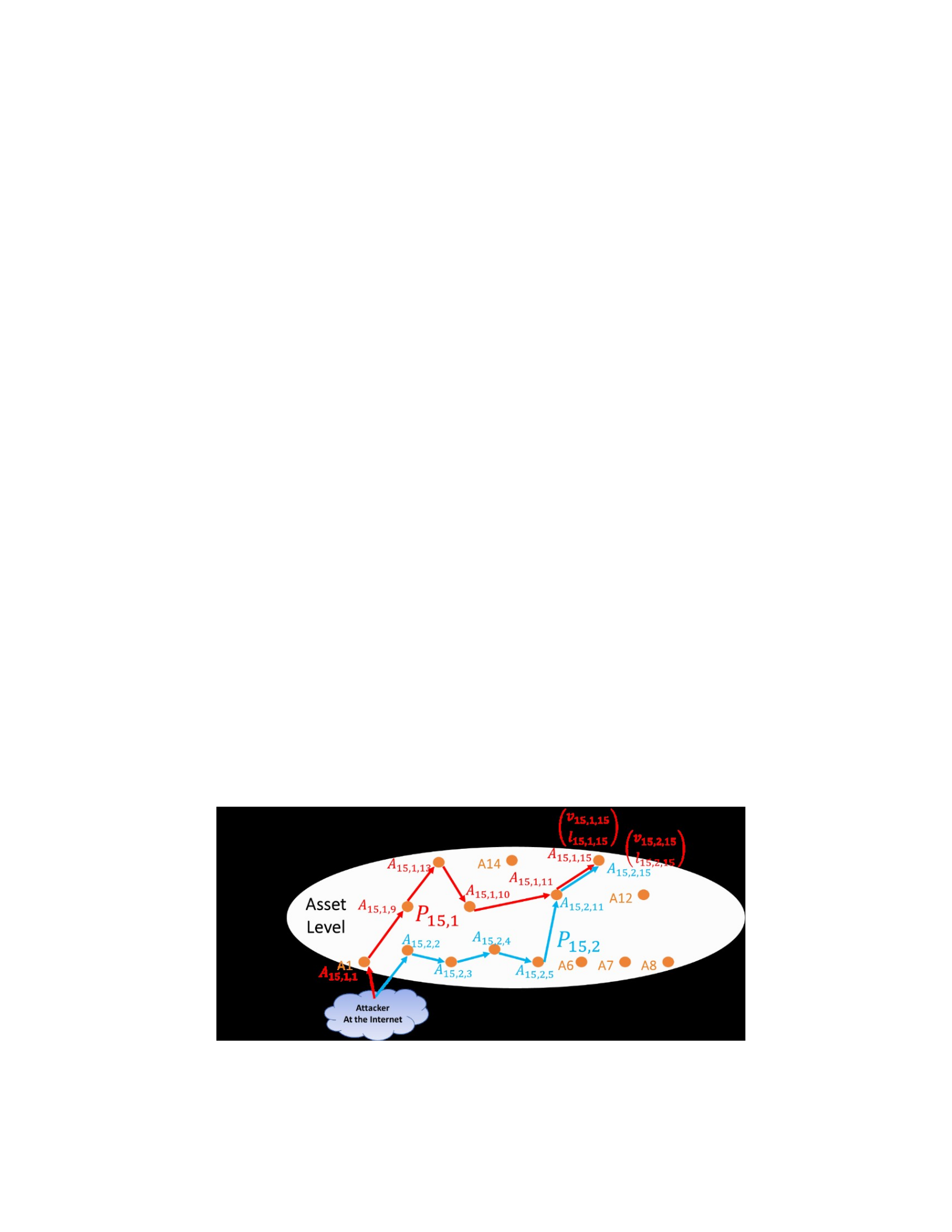
90
5. 𝑙𝑙𝑖𝑖𝑖𝑖𝑘𝑘 likelihood (unconditional probability) value of exploiting the vulnerability 𝐴𝐴𝑖𝑖𝑖𝑖𝑘𝑘 on
asset 𝑅𝑅
Each row of the table represents another vulnerability and its likelihood value on each
asset of each attack path of each attack graph. Table 11 presents the output of the example case in
Chapter 5.
These outputs of the integration function become the inputs of the Impact Graph at the
asset layer along with some other inputs such as CIA requirements of CVSS environmental
metrics and functional dependency topology and parameters.
In Figure 22, an example attack graph is presented. It shows all 15 assets of the
enterprise. This attack graph is developed as the target asset is Asset 15, 𝐴𝐴15. Therefore, the
attack graph is named 𝐴𝐴𝐴𝐴15. It consists of two attack paths, 𝑃𝑃15,1 and 𝑃𝑃15,2. Other
attack paths should be generated for each possible target asset for a complete analysis.
Figure 22.
Two attack paths of an example attack graph

91
The attack graph – impact graph integration function delivers all necessary information
from these two paths to the impact graph, including the list of the assets in the path, the exploited
vulnerabilities, and their likelihood values. The integration of 𝑃𝑃15,1 with the impact graph is
visualized in Figure 23. This attack path is established on six assets:
𝐴𝐴15,1,1, 𝐴𝐴15,1,9, 𝐴𝐴15,1,13, 𝐴𝐴15,1,10, 𝐴𝐴15,1,11, 𝐴𝐴15,1,15
The impact graph in Figure 23 represents the impact propagation caused by this attack
path by red arrows starting from the indicated six assets and eventually affecting all four
Business Processes.
Figure 23.
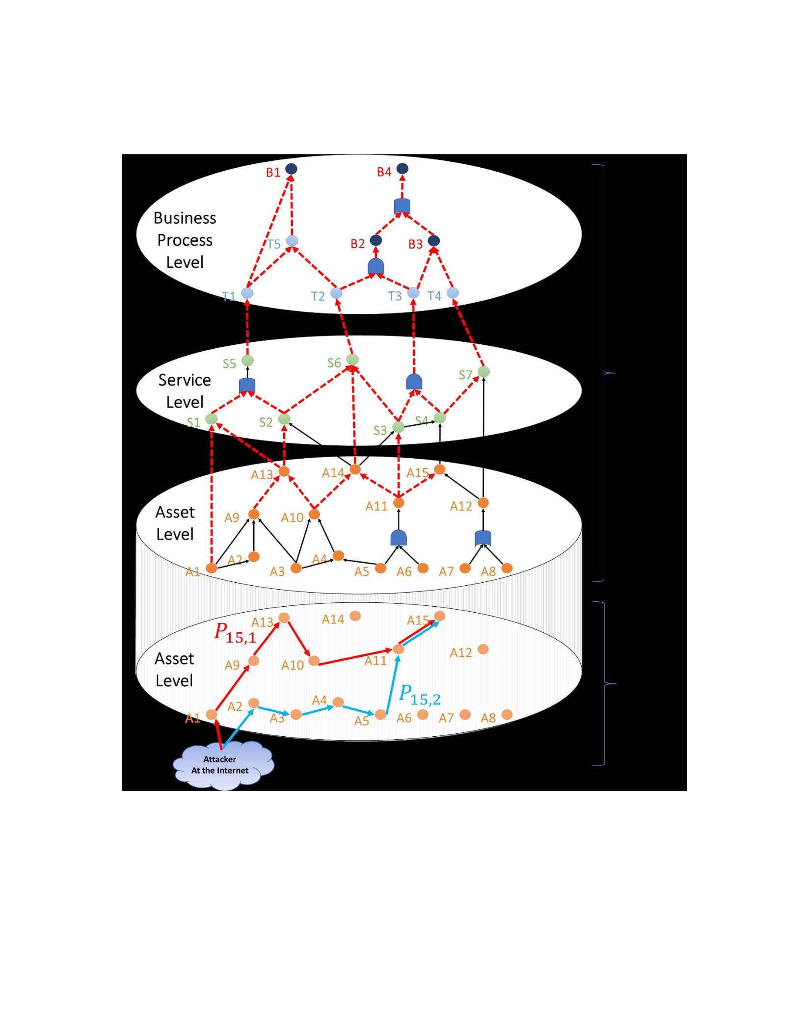
92
Visualization of the differences of attack propagation and impact propagation
The Formula for Calculating Total Cost
In this study, the formula for calculating the loss of impact of FDNA-Cyber is modified to
implement the time-dependency feature. FDNA-Cyber suggests that there are 13 cost items of an

93
adverse cyber event: (1) Loss of data and equipment, (2) Loss of revenue, (3) Loss of strategic
information, (4) Reputational damage, (5) Cybersecurity improvements, (6) Public Relations, (7)
Regulatory penalties, (8) Court settlement fees, (9) Forensics, (10) Loss of Intellectual Property,
(11) Increased cost of capital, (12) Customer protection, and (13) Breach notification, (Table 9)
(Tatar, 2019).
While some of the cost items are one-time costs, Loss of Revenue and Loss of Data and
Equipment are time-dependent cost items. In order to implement the time dependency effect of
these cost items, the total cost equation is modified.
Table 9.
Relation of potential consequences, cost factors (confidentiality, integrity, and availability), and time
dependency multipliers
Cost Item
Number Cost/Loss Item
Cost Parameter
C I A
Time Dependency
Multiplier
𝒍𝒍 𝑪𝑪𝒍𝒍𝑩𝑩𝒊𝒊 𝑰𝑰𝒍𝒍𝑩𝑩𝒊𝒊
𝑨𝑨𝒍𝒍𝑩𝑩𝒊𝒊 𝒎𝒎𝒍𝒍𝑩𝑩𝒊𝒊(𝒕𝒕)
1 Loss of Data and Equipment 𝐶𝐶1𝐵𝐵𝑖𝑖 𝐼𝐼1𝐵𝐵𝑖𝑖 𝐴𝐴1𝐵𝐵𝑖𝑖 𝑖𝑖1𝐵𝐵𝑖𝑖(𝑖𝑖)

94
The total cost equation with time unit as an hour can be generalized as follows:
𝑘𝑘𝑡𝑡=𝑒𝑒𝑛𝑛𝑒𝑒
𝑇𝑇𝑆𝑆𝑇𝑇𝐴𝐴𝑇𝑇 𝐶𝐶𝑆𝑆𝑆𝑆𝑇𝑇 = 𝐶𝐶𝑜𝑜𝑅𝑅𝑖𝑖(𝐵𝐵𝑖𝑖, 𝑖𝑖, 𝑅𝑅(𝑖𝑖))
𝑖𝑖=1 𝑡𝑡=𝑠𝑠𝑡𝑡𝑠𝑠𝑠𝑠𝑡𝑡
(Equation 5)
Where 𝐵𝐵𝑖𝑖 is a Business Process: 𝑖𝑖 = 1, 2, … , 𝑅𝑅,
𝑖𝑖 is the time unit (e.g., ℎ𝑜𝑜𝑜𝑜𝐴𝐴, 𝑜𝑜𝑖𝑖𝐸𝐸, 𝐸𝐸𝑙𝑙𝑖𝑖𝐴𝐴), 𝑖𝑖 receives all values from scenario
𝑅𝑅𝑖𝑖𝑖𝑖𝐴𝐴𝑖𝑖

95
time to scenario 𝑙𝑙𝑀𝑀𝑜𝑜 time.
𝑅𝑅 is the binary variable that indicates incident start time.
The cost function is the main component of the Total Cost equation. Parameters are presented
in Table 9.
𝐶𝐶𝑜𝑜𝑅𝑅𝑖𝑖 (𝐵𝐵𝑖𝑖, 𝑖𝑖, 𝑅𝑅(𝑖𝑖)) = 𝑓𝑓(𝐶𝐶𝐵𝐵𝑖𝑖, 𝑖𝑖, 𝑅𝑅(𝑖𝑖), 𝐼𝐼𝐵𝐵𝑖𝑖, 𝑖𝑖, 𝑅𝑅(𝑖𝑖), 𝐴𝐴𝐵𝐵𝑖𝑖,
𝑖𝑖, 𝑅𝑅(𝑖𝑖))
2 13
𝐶𝐶𝐵𝐵𝑖𝑖 = 𝐶𝐶𝑙𝑙𝐵𝐵𝑖𝑖𝑚𝑚𝑠𝑠𝑚𝑚 ∗ 𝑖𝑖𝑙𝑙𝐵𝐵𝑖𝑖(𝑖𝑖) + 𝐶𝐶𝑙𝑙𝐵𝐵𝑖𝑖
𝑙𝑙=1 𝑙𝑙=3
𝐶𝐶𝐵𝐵𝑖𝑖 = 𝐶𝐶1𝐵𝐵𝑖𝑖𝑚𝑚𝑠𝑠𝑚𝑚 ∗ 𝑖𝑖1𝐵𝐵𝑖𝑖(𝑖𝑖) + 𝐶𝐶2𝐵𝐵𝑖𝑖𝑚𝑚𝑠𝑠𝑚𝑚 ∗ 𝑖𝑖2𝐵𝐵𝑖𝑖(𝑖𝑖) + 𝐶𝐶3𝐵𝐵𝑖𝑖 +
𝐶𝐶4𝐵𝐵𝑖𝑖 + 𝐶𝐶5𝐵𝐵𝑖𝑖 + 𝐶𝐶6𝐵𝐵𝑖𝑖 + 𝐶𝐶7𝐵𝐵𝑖𝑖 + 𝐶𝐶8𝐵𝐵𝑖𝑖
+ 𝐶𝐶9𝐵𝐵𝑖𝑖 + 𝐶𝐶10𝐵𝐵𝑖𝑖 + 𝐶𝐶11𝐵𝐵𝑖𝑖 + 𝐶𝐶12𝐵𝐵𝑖𝑖 + 𝐶𝐶13𝐵𝐵𝑖𝑖
2 9
𝐼𝐼𝐵𝐵𝑖𝑖 = 𝐼𝐼𝑙𝑙𝐵𝐵𝑖𝑖𝑚𝑚𝑠𝑠𝑚𝑚 ∗ 𝑖𝑖𝑙𝑙𝐵𝐵𝑖𝑖(𝑖𝑖) + 𝐼𝐼𝑙𝑙𝐵𝐵𝑖𝑖
𝑙𝑙=1 𝑙𝑙=3
𝐼𝐼𝐵𝐵𝑖𝑖 = 𝐼𝐼1𝐵𝐵𝑖𝑖𝑚𝑚𝑠𝑠𝑚𝑚 ∗ 𝑖𝑖1𝐵𝐵𝑖𝑖(𝑖𝑖) + 𝐼𝐼2𝐵𝐵𝑖𝑖𝑚𝑚𝑠𝑠𝑚𝑚 ∗ 𝑖𝑖2𝐵𝐵𝑖𝑖(𝑖𝑖) + 𝐼𝐼3𝐵𝐵𝑖𝑖 +
𝐼𝐼4𝐵𝐵𝑖𝑖 + 𝐼𝐼5𝐵𝐵𝑖𝑖 + 𝐼𝐼6𝐵𝐵𝑖𝑖 + 𝐼𝐼7𝐵𝐵𝑖𝑖 + 𝐼𝐼8𝐵𝐵𝑖𝑖 + 𝐼𝐼9𝐵𝐵𝑖𝑖
2 9
𝐴𝐴𝐵𝐵𝑖𝑖 = 𝐴𝐴𝑙𝑙𝐵𝐵𝑖𝑖𝑚𝑚𝑠𝑠𝑚𝑚 ∗ 𝑖𝑖𝑙𝑙𝐵𝐵𝑖𝑖(𝑖𝑖) + 𝐴𝐴𝑙𝑙𝐵𝐵𝑖𝑖
𝑙𝑙=1 𝑙𝑙=3
𝐴𝐴𝐵𝐵𝑖𝑖 = 𝐴𝐴1𝐵𝐵𝑖𝑖𝑚𝑚𝑠𝑠𝑚𝑚 ∗ 𝑖𝑖1𝐵𝐵𝑖𝑖(𝑖𝑖) + 𝐴𝐴2𝐵𝐵𝑖𝑖𝑚𝑚𝑠𝑠𝑚𝑚 ∗ 𝑖𝑖2𝐵𝐵𝑖𝑖(𝑖𝑖) +
𝐴𝐴3𝐵𝐵𝑖𝑖 + 𝐴𝐴4𝐵𝐵𝑖𝑖 + 𝐴𝐴5𝐵𝐵𝑖𝑖 + 𝐴𝐴6𝐵𝐵𝑖𝑖 + 𝐴𝐴7𝐵𝐵𝑖𝑖 + 𝐴𝐴8𝐵𝐵𝑖𝑖
+ 𝐴𝐴9𝐵𝐵𝑖𝑖

96
Where 𝐵𝐵𝑖𝑖 is a Business Process: 𝑖𝑖 = 1, 2, … , 𝑅𝑅,
𝑖𝑖 is the time unit (e.g., ℎ𝑜𝑜𝑜𝑜𝐴𝐴, 𝑜𝑜𝑖𝑖𝐸𝐸, 𝐸𝐸𝑙𝑙𝑖𝑖𝐴𝐴), 𝑖𝑖 receives all values from scenario
𝑅𝑅𝑖𝑖𝑖𝑖𝐴𝐴𝑖𝑖
time to scenario 𝑙𝑙𝑀𝑀𝑜𝑜 time.
𝑅𝑅(𝑖𝑖) binary variable indicating if the attack starts at the current period: 1, for incident
start time; 0, otherwise.
𝐶𝐶𝐵𝐵𝑖𝑖 is the cost of loss of confidentiality for 𝐵𝐵𝑖𝑖,
𝐼𝐼𝐵𝐵𝑖𝑖 is the cost of loss of integrity for 𝐵𝐵𝑖𝑖,
𝐴𝐴𝐵𝐵𝑖𝑖 is the cost of loss of availability for 𝐵𝐵𝑖𝑖,
𝑙𝑙 is the cost item number: 𝑙𝑙 = 1,2, … ,13,
ClBi is the estimated loss amount for confidentiality component of cost item 𝑙𝑙 for
Business Process 𝑖𝑖,
IlBi is the estimated loss amount for integrity component of cost item 𝑙𝑙 for Business
Process 𝑖𝑖,
AlBi is the estimated loss amount for availability component of cost item 𝑙𝑙 for
Business Process 𝑖𝑖,
mlBi(t) is the time dependency multiplier defined by the user,
𝐶𝐶𝑙𝑙𝐵𝐵𝑖𝑖𝑚𝑚𝑠𝑠𝑚𝑚 is the estimated maximum loss amount for confidentiality component of
cost item 𝑙𝑙 for Business Process 𝑖𝑖,
𝐼𝐼𝑙𝑙𝐵𝐵𝑖𝑖𝑚𝑚𝑠𝑠𝑚𝑚 is the estimated maximum loss amount for integrity component of cost item

97
𝑙𝑙 for Business Process 𝑖𝑖,
𝑅𝑅(𝑖𝑖) is a binary variable used during the computation process to indicate the scenario
start time since cost items other than Loss of Revenue and Loss of Data and Equipment are one-
time costs and apply only at the start time of an attack. Only these two cost items receive the
value one after the start time. The equation is as follows:
1, 𝑖𝑖 = 𝑅𝑅𝑖𝑖𝑖𝑖𝐴𝐴𝑖𝑖
𝑅𝑅(𝑖𝑖) = 1, 𝑖𝑖 ≠ 𝑅𝑅𝑖𝑖𝑖𝑖𝐴𝐴𝑖𝑖 𝑜𝑜𝑀𝑀𝑙𝑙𝐸𝐸 𝑓𝑓𝑜𝑜𝐴𝐴 𝐶𝐶𝑜𝑜𝑅𝑅𝑖𝑖 𝑖𝑖𝑖𝑖𝑙𝑙𝑖𝑖𝑅𝑅
1 𝑖𝑖𝑀𝑀𝑜𝑜 2
0, 𝑜𝑜𝑖𝑖ℎ𝑙𝑙𝐴𝐴𝑤𝑤𝑖𝑖𝑅𝑅𝑙𝑙
Before starting analyzing risk, the cost estimates for each Business Process should be
completed, including ClBi, IlBi, AlBi, 𝐶𝐶𝑙𝑙𝐵𝐵𝑖𝑖𝑚𝑚𝑠𝑠𝑚𝑚, 𝐼𝐼𝑙𝑙𝐵𝐵𝑖𝑖𝑚𝑚𝑠𝑠𝑚𝑚, and 𝐴𝐴𝑙𝑙𝐵𝐵𝑖𝑖𝑚𝑚𝑠𝑠𝑚𝑚
values. 𝑖𝑖𝑙𝑙𝐵𝐵𝑖𝑖(𝑖𝑖) values should
be assigned for the time-dependent cost items in accordance with the maximum estimate values of
the relevant cost items. The example implementation is presented in Chapters 5 and 6.
CHAPTER 5
IMPLEMENTATION OF THE MODEL
Introduction
This chapter presents a practical perspective on the developed model for the potential
users of the model. The following sections provide a discussion on who would benefit from the
developed model, explain the details of the aspects of the model that help customize the model to
apply to an organization, list the specific actions to be made sequentially in order to apply the

98
developed model, and present an example of applying the developed model on a simple network
of an education institute.
Uses of the Model
This is a generalizable model that can be applied to various organizations in diverse
sectors. Among others, enterprise decision-makers and actuaries/insurance companies are the
possible users that would benefit most:
For enterprise decision-makers, this model can help well-informed cyber risk
management decisions. Moreover, using this model can help simulate and analyze various cyber-
attack scenarios on the organization’s network without risking any interruption on the operations.
For insurance companies and actuaries, this model can help calculate the Total Insurable
Value of an enterprise by estimating the Insured’s Property Value and the Insured’s Time Element.
Adapting the Model to an Enterprise
In order to implement this model, all relevant inputs should be employed along with
adjusting the model’s inputs that are the features that help to customize it to the organizations
with distinct characteristics. Metric values provided with this model should not be considered the
only inputs of the developed model to solve the problem of quantifying the cyber risks of any
enterprise. There are multiple ways of customizing the model based on the characteristics of the
company profile in consideration. The developed model includes a multiple-step approach to
modify the inputs of calculations that must be conducted for the specific enterprise network
under consideration. In other words, the numbers provided within the developed model are not
the only inputs for the analyses to be conducted while employing the model on an enterprise ICT
network.

99
The features of the model that helps customize the inputs are summarized below:
1. Environmental Metric Group of CVSS
a. Modified Base Metrics
b. Confidentiality Requirement, Integrity Requirement, Availability Requirement
2. Features of the impact graph analyses
a. Nodes
b. Dependency relations
c. Type of the dependency relations
d. Dependency parameters
e. Defining time unit
f. Determining time-dependent Strength of Dependency relations
g. Determining time-dependent cost items
h. Determining probabilistic inputs
3. Weights of confidentiality, integrity, and availability constituent nodes
The inputs of the model that helps customization are explained in detail in the following
subsections.
Environmental Metric Group of CVSS
Modified Base Metrics. The environmental metric group is included to address the
differences among the characteristics of vulnerabilities of ICT network components from
individual enterprises that belong to various industries/sectors and at different sizes. The
Modified Base Metrics include all metrics within the Base Metric Group as a means to customize
inputs based on the intrinsic characteristics of the asset within the enterprise under consideration.

100
For example, exploiting a specific vulnerability typically can be done if the computer is
connected to a network. Therefore, the Attack Vector metric for this software is Network.
Suppose that the enterprise under consideration has an isolated intranet that is not connected to
the internet, and the targeted asset has this vulnerability. Since the asset is not connected to the
internet, an attacker needs physical access to at least one of the computers within the intranet.
This situation can be handled by adjusting the Modified Attack Vector metric to Local.
If the target asset is not connected to any network and there is no network connection
device integrated, the only way to exploit such vulnerability is by having physical access to the
asset itself. In this case, the Modified Attack Vector metric becomes Physical.
Modifications similar to the ones in the examples can be made on other Modified Base
Metrics to reflect characteristics of vulnerabilities on the ICT components of the enterprise.
Confidentiality Requirement, Integrity Requirement, Availability Requirement.
There are three other metrics in the Environmental Metric Group that help evaluate a
vulnerability on an ICT component: Confidentiality Requirement, Integrity Requirement, and
Availability Requirement. The exact same vulnerability on a network-connected ICT component
may significantly impact confidentiality, integrity, or availability. However, it may have no or
lower effect if exploited on another component. These metrics are supposed to be used to adjust
for such differences. For example, for a vulnerability on a web server that all of its content is
publicly available, an exploit that only affects its confidentiality is not important since there is no
confidential data in the server. In this case, the Confidentiality Requirement for the
vulnerabilities of this ICT component is set to Low.

101
Features of Impact Graph Analyses
Some features of Functional Dependency Network Analysis provide the ability to
integrate better the characteristics of an enterprise’s ICT network to the analyses. These features
are its nodes, dependency relations, type of dependency relations, and dependency parameters.
Even small changes in these may affect the behavior of the model. Building the functional
dependency network is an essential step of the developed model to implement the characteristics
of the enterprise ICT network.
Nodes. Nodes of Functional Dependency Network Analysis are not necessarily are
individual components of a network. Each asset might be represented by multiple nodes within
the functional dependency network if they have more than one function within the network.
Nodes also help simplify the assets with complicated features. While it is possible to
represent a workstation that is rarely used as a node, it is also possible to assign an industrial
control system that manages the cooling water flow of a reactor as another node. Regardless of
how complicated an asset’s design is or how vital its operation is, the functionality of the asset
turns into a node within the functional dependency network. A person does not need to know
every detail of how an ICT asset works; knowing what functionality the asset provides is enough
to identify the node of the functional dependency network.
Dependency Relations. All processes of an enterprise can be modeled as a part of the
functional dependency network of the enterprise. The functional dependency relation does not
necessarily follow the input-output relations among the nodes of the enterprise. In other words,
products or information may flow from one asset to another, but functional dependency may follow
the inverse flow among the functionalities of these nodes. For example, a feedback loop in a process

102
can be modeled as functionality to check and improve the quality of the product. The loop in the
information flow may be modeled as a functional dependency relation from the node of the feedback
mechanism to the production process.
Type of Dependency Relations. In the developed model, in addition to the dependency
relation of FDNA, there are AND and OR logic dependencies. These dependency types help
implement characteristics of ICT functional dependencies within the analyses. For example, there
is redundancy on a particular system in case one of them has failed to operate; an OR
dependency exists among these redundant nodes and their receiver node.
Dependency Parameters. Strength of Dependency and Criticality of Dependency defines
the level of dependency between two nodes. Their parameters are alpha and beta, respectively.
These two parameters exist for each dependency relation and are other ways of implementing the
characteristics of an enterprise within the analyses.
Defining Time Unit. The developed model can also be tailored for an organization using
time-dependent inputs. The time unit for conducting the analyses can be designated according to
the characteristics of the organization. While it is possible to employ units like an hour, day,
week, month, and year, custom periods can be designated such as three-day, two-week, holiday
season, and tax season. The characteristics of the organization and the analyses to be conducted
are the factors that affect the time unit selection process for each organization.
The Strength of Dependency Relation can be Time-Dependent. Determining the
timedependent Strength of Dependency relations among Services and Business Processes is a way to
customize the model according to the characteristics. Not all operations are conducted at a constant

103
pace and have a constant contribution to the value of an organization. These kinds of differences in
the dependency relationships can be modeled using this feature.
Determining Time-Dependent Cost Items. Revenue and the amount of information
exchanged are unique variables for each organization. While estimating the total loss caused by
an attack, everything should be taken into consideration. Loss of revenue and loss of data and
equipment estimates should be conducted for the organization under focus.
Determining Probabilistic Inputs. Some inputs of the developed model, such as
timedependent strength of dependency, loss of revenue, and loss of data and equipment, can be
probabilistic. If the historical data or forecasts fit a probabilistic distribution, the developed
model can use these inputs for the risk analysis. It is also possible to provide the model a range of
values for operability values on some assets and receive a probability density function as a result
of the analyses.
Weights of Confidentiality, Integrity, and Availability Constituent Nodes
Each node of the developed model is a constituent node with confidentiality, integrity, and
availability components. This is a fundamental characteristic of this model. The operability
values of each component for a node represent how secure a node is from a confidentiality,
integrity, and availability perspective. Each node has an operability value for each of these
components. However, the differences among various types of nodes are represented by the
weights of these components of each constituent node. A higher weight is assigned if one of the
CIA components has high importance for the purpose of the function of the asset. For example, if
the availability of an asset is more important than confidentiality and integrity, a higher weight is
assigned to availability. Weights can be determined by consulting expert opinion. By assigning

104
weights based on the characteristics of a specific asset, the model is customized for the
enterprise.
Model Implementation Sequence
In this section, a sequence to follow in order to employ the developed model efficiently is
presented. The sequence is as follows:
1. Generate the Impact Graph
a. List all Business Processes of the enterprise
b. List all Services that help Business Processes to operate
c. List all assets of the organization
d. Designate the functional dependencies among Assets, Services, and Business
Processes, including interdependencies and intra-dependencies
e. Determine the functional dependency parameters for each dependency
f. Designate time unit
g. Determine the time-dependent and probabilistic variables
h. Make cost estimates
2. Generate Attack Graph
a. Scan all assets to list all the vulnerabilities
b. Generate attack graphs for all possible target assets
3. Analyze Attack Graph
a. Compute conditional probabilities for each node
b. Compute likelihood (unconditional probability) for each node
4. Develop Scenarios

105
5. Analyze Impact Graph for each attack path
a. Employ Attack Graph – Impact Graph Integration Function
b. Retrieve output of the Attack Path
c. Determine inputs for a cost estimate
d. Compute modified metrics for analyses
e. Analyze impact propagation among layers
f. Calculate the loss of impact for the attack path
6. Aggregate and compare results
Example of Implementation of the Model
This section provides a relatively simple example of implementing the developed model
by applying it to a hypothetical online education scenario to help understand the details of the
model. The network topology for the organization is presented in Figure 24. There are two
networks within this topology: Demilitarized Zone (DMZ) and Internal Network. External and
Internal Firewalls control access to Demilitarized Zone. DMZ is used for the operations of the
Web Server. Database Server is located in the Internal Network, which is behind the Internal
Firewall that has more strict firewall rules for access control.
Figure 24.
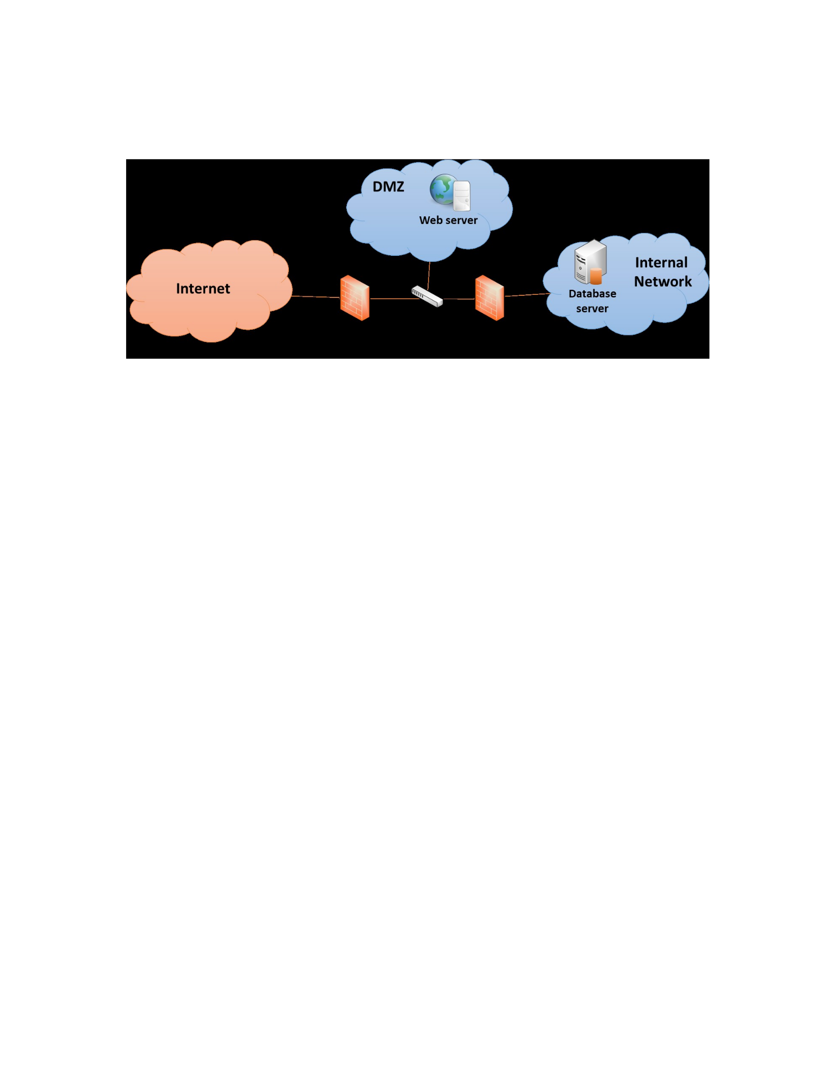
106
Network topology of the organization of the example
Generate the Impact Graph
A top-down approach can be used to generate the impact graph of an enterprise. The
graph consists of nodes and connections where nodes are functional components of the
enterprise, and the connections represent the dependencies among the functions.
An enterprise may have one or multiple business processes, which are the primary goals
of the enterprise to generate value or profit. For a higher education institute that has online
programs, business processes may include “delivering online programs,” “delivering on-site
programs,” and “conducting research activities.” “Delivering online programs” is the business
process focused on in this example and denoted with B1.
The services are the capabilities that help realize the business processes. “Hosting a
website for the archived courses,” “facilitating synchronous courses,” “learning management
system,” “email service” are some of the example services that help enable the institute to deliver
online programs. “Hosting a website for the archived courses” is denoted with S1.
The number of assets is not necessarily the count of hardware of the enterprise. The assets
should be considered from a functional perspective as a specific network component may serve
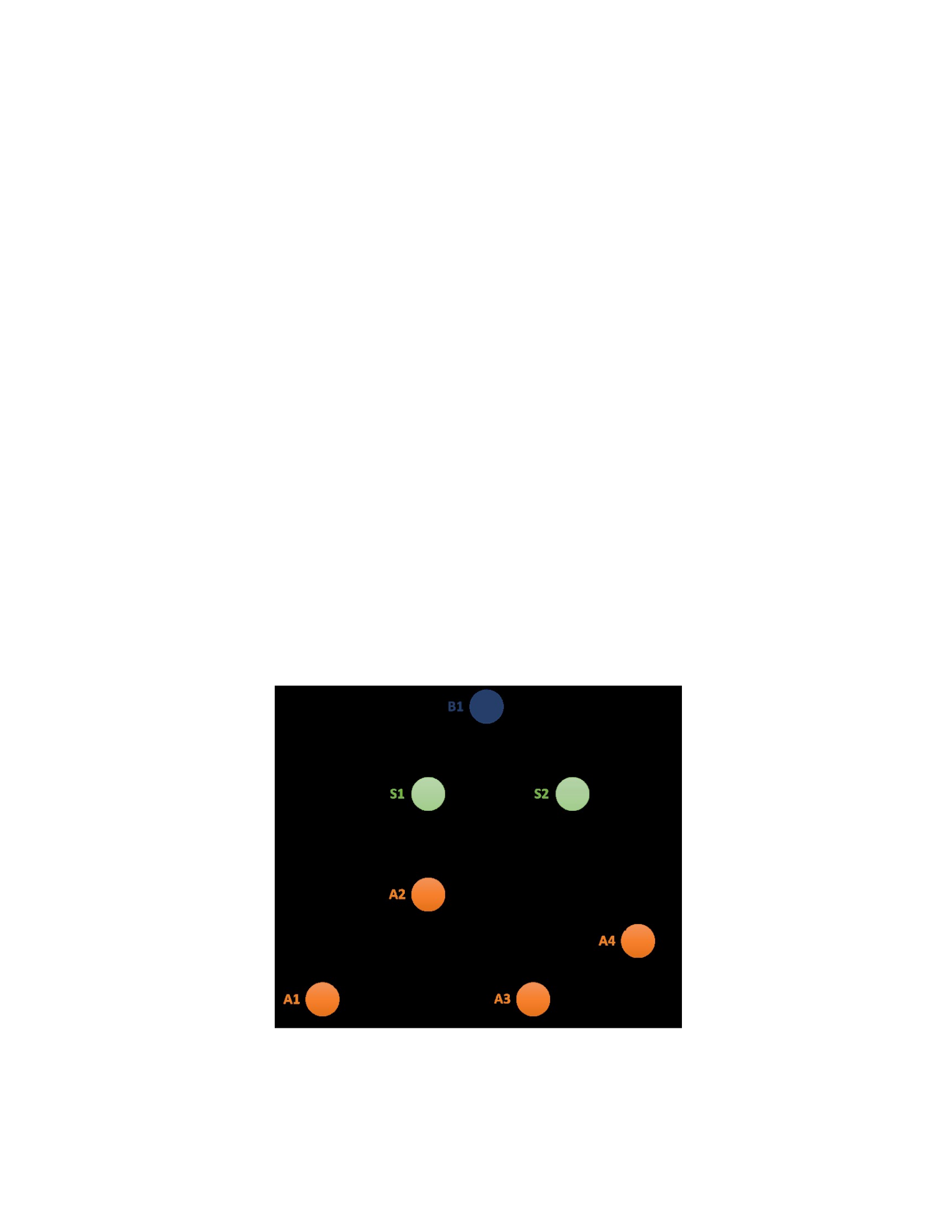
107
in multiple ways with the software programs installed or processes that are supposed to conduct.
The assets that make S1 possible are “external firewall,” web server,” “internal firewall,” and
“database server” and denoted with A1, A2, A3, and A4, respectively.
Listing all business processes, services, and assets is the first step in generating the impact
graph. The next step is providing the dependency relationships among the business processes,
services, and assets. The same top-down approach may be used, while a bottom-up approach can
be used, as well. The functional dependencies within and among the layers should be considered,
including the AND and OR dependencies. Figure 25 presents a part of the impact graph for the
example institution. S1 is only one of the services that support B1; however, this example is kept
simple since it suffices to show how the impact graph works.
Figure 25.
Impact graph for the example

108
All nodes in this impact graph are constituent nodes that consist of confidentiality,
integrity, and availability aspects, and each has a weight according to their importance for each
node. Weights can be determined according to expert opinion. Descriptions and weights for each
node are presented in Table 10.
Table 10.
Impact graph nodes' CIA weights and descriptions
Name Type 𝒘𝒘𝑪
𝑪𝒊𝒊
𝒘𝒘𝑰
𝑰𝒊𝒊
𝒘𝒘𝑨
𝑨𝒊𝒊
Description
A1 External Firewall Asset 0.10 0.45 0.45 Filters traffic to the web server
A2 Web Server Asset 0.10 0.20 0.70 Hosts website for archived online
courses
A3 Internal Firewall Asset 0.10 0.45 0.45 Filters traffic between web and
database servers
A4 Database Server Asset 0.35 0.35 0.30 Archive of online course videos
and
files
S1 Web Hosting
(Archive)
Service 0.20 0.30 0.50
Delivery of an up and running
website with historical online
course contents
B1 Delivering
Online Programs
Business
Process
0.10 0.45 0.45 Delivering online education to
higher education students

109
The final step of generating the impact graph is determining the strength and criticality of
dependency values (alpha and beta parameters) of the dependency connections. The definitions
to recall are as follows:
Strength of Dependency (SOD): “The strength with which a receiver node’s operability level
relies on the operability level of feeder nodes. SOD captures the effects of relationships that increase
the performance as addition to BOL” (Garvey & Pinto, 2009). The parameter for Strength of
Dependency is 𝛼𝛼, and its range is 0 < 𝛼𝛼𝑖𝑖𝑖𝑖 ≤ 1.
Criticality of Dependency (COD): “The criticality of feeder node contributions to a
receiver node for it to achieve its operability level objectives. COD governs how the performance
of the receiver node will decrease below the BOL in time and possible become inoperable
eventually” (Garvey & Pinto, 2009). The parameter for Criticality of Dependency is 𝛽𝛽, and its
range is 0 ≤ 𝛽𝛽𝑖𝑖𝑖𝑖 ≤ 100(1 − 𝛼𝛼𝑖𝑖𝑖𝑖).
Table 11 and Table 12 provide the alpha and beta values between the dependency among CIA
aspects of constituent nodes where each row represents a feeder node while each column
stands for a receiver node. For example, 𝛼𝛼𝐴𝐴1𝐼𝐼,𝐴𝐴2𝐼𝐼 is 0.5 while 𝛽𝛽𝐴𝐴1𝐼𝐼,𝐴𝐴2𝐼𝐼 is 50. These
values are
assigned according to expert evaluation. A1 and A3 columns are empty since they are only feeder
nodes, i.e., not a receiver node. Similarly, B1 rows are empty since B1 is only a receiver node,
not a feeder node.
Table 11.

110
Strength of dependency between feeder (rows) and receiver (columns) node pairs
A1C A1I A1A A2C A2I A2A A3C A3I A3A A4C A4I A4A S1C S1I S1A B1C B1I B1A
A1C 0.3
A1I 0.3 0.5 0.9
A1A
0.8
A2C
1
A2I
1 1 1
A2A
1
A3C 0.8
0.8
A3I 0.9 0.8 0.5 1 0.9 0.5
A3A
0.3 0.5
A4C 0.5
A4I 0.1 1 0.1
A4A
0.1
S1C
0.4
S1I
0.4 0.4 0.4
S1A
B1C
0.4

111
B1I
B1A
Table 12.
Criticality of dependency between feeder (rows) and receiver (columns) node pairs
A1C A1I A1A A2C A2I A2A A3C A3I A3A A4C A4I A4A S1C S1I S1A B1C B1I B1A
A1C 50
A1I 50 50
10
A1A
10
A2C
0
A2I
0 0 0
A2A
0
A3C 20
20
A3I 10 20
30 0 10 50
A3A
30
50
A4C 25
A4I 50 0
80
A4A
85
S1C
60
S1I
55 60 55

112
S1A
B1C
B1I
B1A
60
Cost estimates should also be completed in order to conduct the analyses. Time-
dependent cost items are Loss of Revenue and Loss of Data and Equipment. Estimates for these
cost items should be conducted to provide a maximum number so that the average number
should be approximately 0.3-0.4 times the estimated maximum values. This is not a mandatory
rule; however, these estimates should be parallel with the daily multiplier values. In this example,
the multiplier value for the time unit the analyses conducted is 0.4. All other cost estimates
should be conducted to provide an average number per cyber incident. The cost estimate values
for the cost items are presented in Table 13.
Table 13.
Cost estimates for the example
Loss of Data and Equipment 1 $ 19,565 $ 21,268 $ 17,081
Loss of Revenue 2 $ - $ - $ 234,358
Cost Item Cost Item # C I A

113
Loss of Strategic Information 3 $ - $ - $ -
Reputational Damage 4 $ 3,622 $ 4,251 $ 4,648
Cybersecurity Improvements 5 $ 20,000 $ 30,000 $ 30,000
PR 6 $ 2,681 $ 2,923 $ 3,812
Regulatory Penalties 7 $ - $ - $ -
Court Settlement Fees 8 $ 5,000 $ 5,812 $ 5,000
Forensics 9 $ 4,162 $ 3,363 $ 5,503
Generate the Attack Graph
In order to generate the attack graph, all the assets are needed to be scanned for
vulnerabilities. After scanning the four assets, an attack graph generation software generates
possible attack paths for specific targets. In this example, it is assumed that there is only one
attack path targeting the database server’s availability. The attack graph for such intrusion for an
attacker located on the internet is depicted in Figure 26.
Figure 26.
Loss of IP 10 $ -
Table 13. continued.
Cost Item Cost Item # C I A
Increased Cost of Capital 11 $ -
Customer Protection 12 $ -
Breach Notifications 13 $ -

114
Attack graph for the example
As can be seen, the exploitation of two vulnerabilities is required to disrupt the database
server's operation.
The first vulnerability is on the Web Server (C), and its identifier in NVD is CVE-
20196111 (National Vulnerability Database, 2019d). This vulnerability exists on OpenSSH, a set
of software programs that help secure networking using the Secure Shell Protocol. The
exploitation of this vulnerability can give the attackers the ability to overwrite any files in the
target directory, therefore considered an attack against the integrity of the server. The
confidentiality and availability of the server are not affected by this attack. The details about the
vulnerabilities, based on the National Vulnerability Database, are as follows:
CVSS Values of CVE-2019-6111 on Web Server
Vector String: AV:N/AC:H/PR:N/UI:N/S:U/C:N/I:H/A:N
CVSS Base Score: 5.9 MEDIUM
•Attack Vector (AV): Network
•Attack Complexity (AC): High
•Privileges Required (PR): None
•User Interaction (UI): None
•Scope (S): Unchanged
•Confidentiality (C): None
•Integrity (I): High

115
•Availability (A): None
The second vulnerability exists on the Database Server (A), and its identifier is CVE-
201918601 (National Vulnerability Database, 2019b). This vulnerability exists in a distributed
file system called OpenAFS. Attackers may exploit this vulnerability and gain the ability to send
maliciously repeated calls to the database server that results in the database to crash and cause a
denial of service. Such an attack is considered a complex attack, but it does not require any user
interaction or specific credentials. Moreover, it is possible to conduct this attack remotely from
the internet. The only impact has occurred on the availability of the server, i.e., confidentiality
and integrity of the server are not affected. The details about the vulnerabilities, based on the
National
Vulnerability Database, are as follows:
CVSS Values of CVE-2019-18601 on Database Server
Vector String: AV:N/AC:L/PR:N/UI:N/S:U/C:N/I:N/A:H
CVSS Base Score: 7.5 HIGH
•Attack Vector (AV): Network
•Attack Complexity (AC): Low
•Privileges Required (PR): None
•User Interaction (UI): None
•Scope (S): Unchanged
•Confidentiality (C): None
•Integrity (I): None
•Availability (A): High

116
Analyze Attack Graph
In this example, it is assumed that only one attack graph exists (AG4), and for this attack
graph, there is only one attack path (P4,1) for simplicity. All conditional and unconditional
probabilities are calculated in this step.
Numerical data in Table 14 is determined according to the information on NVD and Table
6. Some of these values will be used in impact analysis and explained later. In this step, the
unconditional probabilities are needed to be calculated using Equation 4. It is assumed that the
probability of an attacker’s desire to attack is 0.5, which is Pr(E).
Table 14.
Numerical values for CVSS metrics for vulnerabilities
CVE-2019-6111 CVE-2019-18601
Metric Value Numerical Value Value Numerical Value
Attack Vector (AV) Network 0.85 Networ
k 0.85
Attack Complexity (AC) High 0.44 Low 0.77
Privileges Required (PR) None 0.85 None 0.85
User Interaction (UI) None 0.85 None 0.85
Scope (S) Unchanged Unchanged
Confidentiality (C) None 100 None 100
Integrity (I) High 0 None 100
Availability (A) None 100 High 0
Remediation Level Temporary fix 0.97
Conditional Probability P(C|D) 0.550428 P(A|B) 0.99304

117
The web server is located in the network topology at a Demilitarized Zone (DMZ). The
external firewall protects the DMZ by letting only the relevant traffic from the internet to the
network. Pr(D|E) is the conditional probability of direct access from the internet to browse the
content published on the web server. Since such traffic is allowed, the probability, Pr(D|E), is
equal to 1.
Pr(𝑆𝑆) = Pr(𝑆𝑆|𝐸𝐸) ∗ Pr(𝐸𝐸) = 1 ∗ 0.5 = 0.5
According to Equation 4, the conditional probability of exploiting the vulnerability on
software that runs on the web server, which is Pr(C|D), is calculated by plugging the values in
Table 14, as follows:
Pr(𝐶𝐶|𝑆𝑆) = 2.1 ∗ Attack Vector ∗ Attack Complexity ∗ Privileges Required ∗ User
Interaction
∗ Exploit Code Maturity ∗ Remediation Level ∗ Report Confidence
= 2.1 ∗ 0.85 ∗ 0.44 ∗ 0.85 ∗ 0.85 ∗ 1 ∗ 0.97 ∗ 1 = 0.55
The unconditional probability of the web server to be exploited is calculated as follows:
Pr(𝐶𝐶) = Pr(𝐶𝐶|𝑆𝑆) ∗ Pr(𝑆𝑆) = 0.55 ∗ 0.5 = 0.28
The impact of exploiting this vulnerability on the web server on integrity is high, and it
provides an attacker the ability to execute arbitrary code on the server. According to the
configurations of the internal firewall, only the web server can access the database server. The
web server is needed to be used as a stepping stone in this attack path. Using this privilege
escalation, the attacker can pass the internal server to exploit the vulnerability on the database

118
server. The conditional probability of multi-hop access at the internal firewall is 1, thus Pr(B|C) =
1. This makes the unconditional probability of internal firewall, Pr(B) = 0.28 * 1 = 0.28.
The conditional probability of exploiting the vulnerability on the database server is also
calculated using Equation 4 and the values in Table 14, as follows:
Pr(𝐴𝐴|𝐵𝐵) = 2.1 ∗ Attack Vector ∗ Attack Complexity ∗ Privileges Required ∗ User
Interaction
∗ Exploit Code Maturity ∗ Remediation Level ∗ Report Confidence
= 2.1 ∗ 0.85 ∗ 0.77 ∗ 0.85 ∗ 0.85 ∗ 1 ∗ 1 ∗ 1 = 0.99
Even if the conditional probability is high, the unconditional probability is much lower since
the database server is located at a better-defended network segment.
Pr(𝐴𝐴) = Pr(𝐴𝐴|𝐵𝐵) ∗ Pr(𝐵𝐵) = 0.99 ∗ 0.28 = 0.27
Given that all unconditional probability values have been calculated, the attack graph –
impact graph integration can be performed. Figure 27 visualizes the integration. The related
nodes of the attack graph and impact graph are connected with dashed orange lines.
Figure 27.
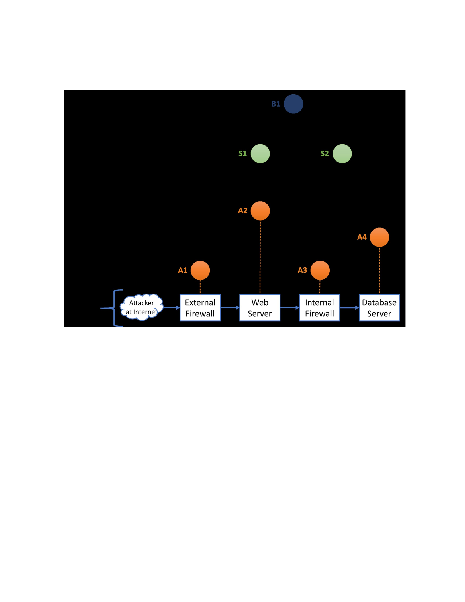
119
Attack graph - impact graph integration example
Note that paths of attack propagation and impact propagation are not the same. While there
is one attack path (A1-A2-A3-A4), there are three impact propagation paths (A1-A2; A3-A2;
A3A4-A2) within the Asset layer. The reason is that the functional dependency among the assets
does not perfectly correlate with the ICT network topology and possible multi-step attacks.
The outputs of the attack graph – impact graph integration function is summarized in
Table 15. In the scope of this example, only A4 was chosen as a target node; thus, there is one
attack graph (AG4). Based on the vulnerabilities within the assets, there is only one attack path
(P4,1). The table also gives related vulnerabilities and the likelihood (unconditional probability)
values for each asset along this attack path.

120
Table 15.
Integration function output table for the example
𝑨𝑨𝑮
𝑮𝒊𝒊
𝑷𝑷𝒊𝒊,
𝒋𝒋
𝑨𝑨𝒊𝒊,𝒋
𝒋,𝒌𝒌
𝒗𝒗𝒊𝒊,𝒋𝒋,𝒌𝒌 𝒍𝒍𝒊𝒊,𝒋𝒋,
𝒌𝒌
AG4 P4,1 A4,1,1 - -
AG4 P4,1 A4,1,2 CVE-2019-6111 0.28
AG4 P4,1 A4,1,3 - -
AG4 P4,1 A4,1,4 CVE-2019-
18601
0.27
Analyze Impact Graph for Each Attack Path
This step focuses on how the impact of cyber-attacks propagates within and among
enterprise layers, starting from assets and going up to business processes. A2 and A4 are the
affected assets from vulnerability exploitation that makes their performance decrease.
According to Table 14, exploitation of A4 has a high availability impact. The
confidentiality and integrity of A4 are not affected directly by the vulnerability exploitation. High
availability impact decreases the operability value of confidentiality constituent node from 100 to
0, a 100 decrease. The expected utility is calculated by multiplying likelihood and impact values.
Since the likelihood of this exploitation, P(A), is 0.27, the loss in expected utility (𝑉𝑉𝐼𝐼𝐴𝐴4)
becomes 100 * 0.27 = 27 utils (decrease). For feeder-only nodes, the operability value is
decreased by 27 utils to apply the cyber-attack's impact. For the nodes that are both receiver and
feeder, this change can be applied by decreasing the self-efficiency of the node. Since A4 is a
node that is both feeder and receiver, its self-efficiency is decreased by 0.27 from 1 to 0.73 while

121
operability values are kept constant. This means that the availability of A4 can only operate with
73% of its performance.
𝑆𝑆𝐸𝐸𝐴𝐴𝐴𝐴4 = 0.73
where 𝑆𝑆𝐸𝐸𝐼𝐼𝐴𝐴4 is the Self-efficiency of the integrity component of Asset 4.
Similarly, according to Table 14, exploitation of A2 has a high integrity impact.
Confidentiality and availability of A2 are not affected directly by the vulnerability exploitation.
The likelihood of this exploitation, P(C), is 0.27. Expected utility decreases 100 * 0.28 = 28 utils.
Since A2 is a node that is both feeder and receiver, its self-efficiency is decreased by 0.28 from 1
to 0.72 while operability values are kept constant.
𝑆𝑆𝐸𝐸𝐼𝐼𝐴𝐴2 = 0.72
where 𝑆𝑆𝐸𝐸𝐼𝐼𝐴𝐴3 is the Self-efficiency of the integrity component of Asset 2.
Given these self-efficiency values, the impact propagation can be computed. This process
starts from the feeder-only nodes, which are A1 and A3. A1’s and A3’s all CIA components are at
100 operability value level.
𝑃𝑃𝑖𝑖 = 𝑤𝑤𝐶𝐶𝑖𝑖𝑉𝑉𝐶𝐶𝑖𝑖 + 𝑤𝑤𝐼𝐼𝑖𝑖𝑉𝑉𝐼𝐼𝑖𝑖 + 𝑤𝑤𝐴𝐴𝑖𝑖𝑉𝑉𝐴𝐴𝑖𝑖
𝑃𝑃𝐴𝐴1 = 𝑤𝑤𝐶𝐶𝐴𝐴1𝑉𝑉𝐶𝐶𝐴𝐴1 + 𝑤𝑤𝐼𝐼𝐴𝐴1𝑉𝑉𝐼𝐼𝐴𝐴1 + 𝑤𝑤𝐴𝐴𝐴𝐴1𝑉𝑉𝐴𝐴𝐴𝐴1
𝑃𝑃𝐴𝐴1 = 0.10 ∗ 100 + 0.45 ∗ 100 + 0.45 ∗ 100 = 100
𝑃𝑃𝐴𝐴3 = 𝑤𝑤𝐶𝐶𝐴𝐴3𝑉𝑉𝐶𝐶𝐴𝐴3 + 𝑤𝑤𝐼𝐼𝐴𝐴3𝑉𝑉𝐼𝐼𝐴𝐴3 + 𝑤𝑤𝐴𝐴𝐴𝐴3𝑉𝑉𝐴𝐴𝐴𝐴3
𝑃𝑃𝐴𝐴3 = 0.10 ∗ 100 + 0.45 ∗ 100 + 0.45 ∗ 100 = 100
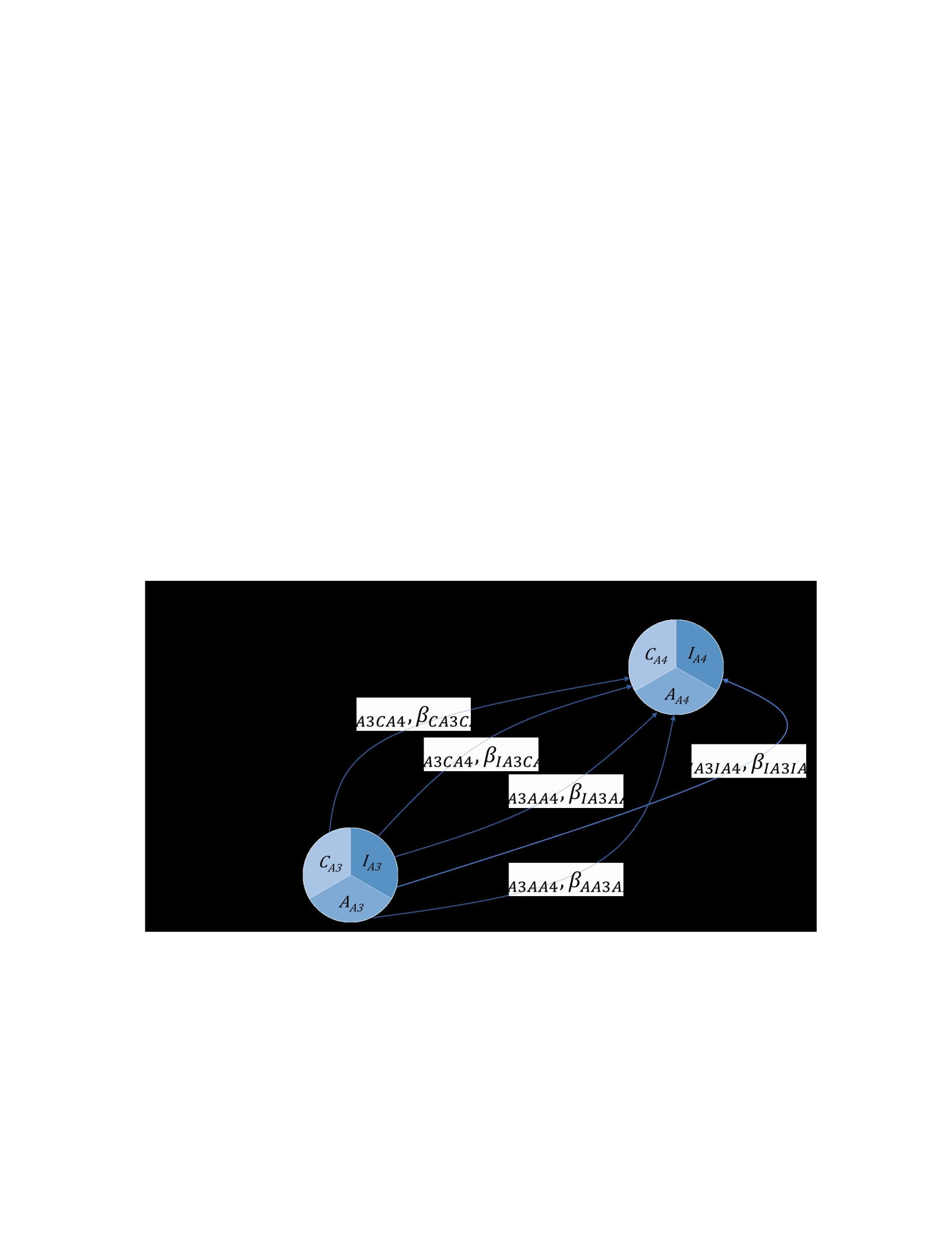
122
Impact propagation calculations are needed to be conducted based on the dependency
network. A1 and A3 feed A2 and A4. Since A2 is dependent on A4, A4’s operability is needed to
be calculated before A2.
𝑃𝑃𝐴𝐴4 = 𝑤𝑤𝐶𝐶𝐴𝐴4𝑉𝑉𝐶𝐶𝐴𝐴4 + 𝑤𝑤𝐼𝐼𝐴𝐴4𝑉𝑉𝐼𝐼𝐴𝐴4 + 𝑤𝑤𝐴𝐴𝐴𝐴4𝑉𝑉𝐴𝐴𝐴𝐴4
A4 is dependent only on one node, A3. The dependency relations among constituent nodes
are shown in Figure 28.
Figure 28.
Dependency relationship between A3 and A4
Below are the equations for one node dependency:
𝑉𝑉𝐶𝐶𝑖𝑖 = 𝑆𝑆𝐸𝐸𝐶𝐶𝑖𝑖 ∗ 𝑀𝑀𝑖𝑖𝑀𝑀𝐴𝐴𝐴𝐴𝑙𝑙𝑆𝑆𝑆𝑆𝑆𝑆𝑉𝑉𝐶𝐶𝑖𝑖𝐶𝐶𝑖𝑖,
𝑆𝑆𝑆𝑆𝑆𝑆𝑉𝑉𝐶𝐶𝑖𝑖𝐼𝐼𝑖𝑖, 𝐶𝐶𝑆𝑆𝑆𝑆𝑉𝑉𝐶𝐶𝑖𝑖𝐶𝐶𝑖𝑖, 𝐶𝐶𝑆𝑆𝑆𝑆𝑉𝑉𝐶𝐶𝑖𝑖𝐼𝐼𝑖𝑖

123
𝛼𝛼𝐶𝐶𝑖𝑖𝐶𝐶𝑖𝑖𝑉𝑉𝐶𝐶𝑖𝑖𝛼𝛼𝐼𝐼𝑖𝑖𝐶𝐶𝑖𝑖𝑉𝑉𝐼𝐼𝑖𝑖𝛼𝛼𝐶𝐶𝑖𝑖𝐶𝐶𝑖𝑖+𝛼𝛼𝐼𝐼𝑖𝑖𝐶𝐶𝑖𝑖
𝑉𝑉𝐶𝐶𝑖𝑖 = 𝑆𝑆𝐸𝐸𝐶𝐶𝑖𝑖 ∗ 𝑀𝑀𝑖𝑖𝑀𝑀 +
+ 100 1 − , 𝑉𝑉𝐶𝐶𝑖𝑖 + 𝛽𝛽𝐶𝐶𝑖𝑖𝐶𝐶𝑖𝑖, 𝑉𝑉𝐼𝐼𝑖𝑖 + 𝛽𝛽𝐼𝐼𝑖𝑖𝐶𝐶𝑖𝑖
2 2 2
𝑉𝑉𝐼𝐼𝑖𝑖 = 𝑆𝑆𝐸𝐸𝐼𝐼𝑖𝑖 ∗ 𝑀𝑀𝑖𝑖𝑀𝑀𝑆𝑆𝑆𝑆𝑆𝑆𝑉𝑉𝐼𝐼𝑖𝑖𝐼𝐼𝑖𝑖, 𝐶𝐶𝑆𝑆𝑆𝑆𝑉𝑉𝐼𝐼𝑖𝑖𝐼𝐼𝑖𝑖 = 𝑆𝑆𝐸𝐸𝐼𝐼𝑖𝑖
∗ 𝑀𝑀𝑖𝑖𝑀𝑀(𝛼𝛼𝐼𝐼𝑖𝑖𝐼𝐼𝑖𝑖𝑉𝑉𝐼𝐼𝑖𝑖 + 1001 − 𝛼𝛼𝐼𝐼𝑖𝑖𝐼𝐼𝑖𝑖, 𝑉𝑉𝐼𝐼𝑖𝑖 + 𝛽𝛽𝐼𝐼𝑖𝑖𝐼𝐼𝑖𝑖)
𝑉𝑉𝐴𝐴𝑖𝑖 = 𝑆𝑆𝐸𝐸𝐴𝐴𝑖𝑖 ∗ 𝑀𝑀𝑖𝑖𝑀𝑀𝐴𝐴𝐴𝐴𝑙𝑙𝑆𝑆𝑆𝑆𝑆𝑆𝑉𝑉𝐴𝐴𝑖𝑖𝐴𝐴𝑖𝑖,
𝑆𝑆𝑆𝑆𝑆𝑆𝑉𝑉𝐴𝐴𝑖𝑖𝐼𝐼𝑖𝑖, 𝐶𝐶𝑆𝑆𝑆𝑆𝑉𝑉𝐴𝐴𝑖𝑖𝐴𝐴𝑖𝑖, 𝐶𝐶𝑆𝑆𝑆𝑆𝑉𝑉𝐴𝐴𝑖𝑖𝐼𝐼𝑖𝑖
𝛼𝛼𝐴𝐴𝑖𝑖𝐴𝐴𝑖𝑖𝑉𝑉𝐴𝐴𝑖𝑖
𝛼𝛼𝐴𝐴𝑖𝑖𝐴𝐴𝑖𝑖+𝛼𝛼𝐼𝐼𝑖𝑖𝐴𝐴𝑖𝑖
𝑉𝑉𝐴𝐴𝑖𝑖 = 𝑆𝑆𝐸𝐸𝐴𝐴𝑖𝑖 ∗ 𝑀𝑀𝑖𝑖𝑀𝑀 +
+ 100 1 − , 𝑉𝑉𝐴𝐴𝑖𝑖 + 𝛽𝛽𝐴𝐴𝑖𝑖𝐴𝐴𝑖𝑖, 𝑉𝑉𝐼𝐼𝑖𝑖 + 𝛽𝛽𝐼𝐼𝑖𝑖𝐴𝐴𝑖𝑖
2 2 2
The operability of A4 and its CIA components can be calculated using these equations as
follows:
𝑉𝑉𝐶𝐶𝐴𝐴4 = 𝑆𝑆𝐸𝐸𝐶𝐶𝐴𝐴4 ∗ 𝑀𝑀𝑖𝑖𝑀𝑀(𝐴𝐴𝐴𝐴𝑙𝑙(𝑆𝑆𝑆𝑆𝑆𝑆𝑉𝑉𝐶𝐶𝐴𝐴4𝐶𝐶𝐴𝐴3,
𝑆𝑆𝑆𝑆𝑆𝑆𝑉𝑉𝐶𝐶𝐴𝐴4𝐼𝐼𝐴𝐴3), 𝐶𝐶𝑆𝑆𝑆𝑆𝑉𝑉𝐶𝐶𝐴𝐴4𝐶𝐶𝐴𝐴3, 𝐶𝐶𝑆𝑆𝑆𝑆𝑉𝑉𝐶𝐶𝐴𝐴4𝐼𝐼𝐴𝐴3)
𝛼𝛼𝐶𝐶𝐴𝐴3𝐶𝐶𝐴𝐴4𝑉𝑉𝐶𝐶𝐴𝐴3𝛼𝛼𝐼𝐼𝐴𝐴3𝐶𝐶𝐴𝐴4𝑉𝑉𝐼𝐼𝐴𝐴3
𝛼𝛼𝐶𝐶𝐴𝐴3𝐶𝐶𝐴𝐴4+𝛼𝛼𝐼𝐼𝐴𝐴3𝐶𝐶𝐴𝐴4
𝑉𝑉𝐶𝐶𝐴𝐴4 = 𝑆𝑆𝐸𝐸𝐶𝐶𝐴𝐴4 ∗ 𝑀𝑀𝑖𝑖𝑀𝑀 +
+ 100 1 − , 𝑉𝑉𝐶𝐶𝐴𝐴3
2 2 2
+ 𝛽𝛽𝐶𝐶𝐴𝐴3𝐶𝐶𝐴𝐴4, 𝑉𝑉𝐼𝐼𝐴𝐴3 + 𝛽𝛽𝐼𝐼𝐴𝐴3𝐶𝐶𝐴𝐴4

124
0.8 𝑉𝑉𝐶𝐶𝐴𝐴4 = 1 𝑀𝑀𝑖𝑖𝑀𝑀
𝑉𝑉𝐶𝐶𝐴𝐴4 = 1𝑀𝑀𝑖𝑖𝑀𝑀(40 + 50 + 100(1 − 0.9), 120,100)
𝑉𝑉𝐶𝐶𝐴𝐴4 = 1𝑀𝑀𝑖𝑖𝑀𝑀(100,120,100)
𝑉𝑉𝐶𝐶𝐴𝐴4 = 100 𝑜𝑜𝑖𝑖𝑖𝑖𝑙𝑙𝑅𝑅
𝑉𝑉𝐼𝐼𝐴𝐴4 = 𝑆𝑆𝐸𝐸𝐼𝐼𝐴𝐴4 ∗ (𝑀𝑀𝑖𝑖𝑀𝑀(𝑆𝑆𝑆𝑆𝑆𝑆𝑉𝑉𝐼𝐼𝐴𝐴4𝐼𝐼𝐴𝐴3,
𝐶𝐶𝑆𝑆𝑆𝑆𝑉𝑉𝐼𝐼𝐴𝐴4𝐼𝐼𝐴𝐴3)
= 𝑆𝑆𝐸𝐸𝐼𝐼𝐴𝐴4 ∗ 𝑀𝑀𝑖𝑖𝑀𝑀(𝛼𝛼𝐼𝐼𝐴𝐴3𝐼𝐼𝐴𝐴4𝑉𝑉𝐼𝐼𝐴𝐴3 + 100(1 −
𝛼𝛼𝐼𝐼𝐴𝐴3𝐼𝐼𝐴𝐴4), 𝑉𝑉𝐼𝐼𝐴𝐴3 + 𝛽𝛽𝐼𝐼𝐴𝐴3𝐼𝐼𝐴𝐴4))
𝑉𝑉𝐼𝐼𝐴𝐴4 = 1 ∗ (𝑀𝑀𝑖𝑖𝑀𝑀(0.9 ∗ 100 + 100(1 − 0.9), 100 + 10))
𝑉𝑉𝐼𝐼𝐴𝐴4 = 𝑀𝑀𝑖𝑖𝑀𝑀(90 + 10,110)
𝑉𝑉𝐼𝐼𝐴𝐴4 = 100 𝑜𝑜𝑖𝑖𝑖𝑖𝑙𝑙𝑅𝑅
𝑉𝑉𝐴𝐴𝐴𝐴4 = 𝑆𝑆𝐸𝐸𝐴𝐴𝐴𝐴4 ∗ 𝑀𝑀𝑖𝑖𝑀𝑀(𝐴𝐴𝐴𝐴𝑙𝑙(𝑆𝑆𝑆𝑆𝑆𝑆𝑉𝑉𝐴𝐴𝐴𝐴4𝐴𝐴𝐴𝐴3,
𝑆𝑆𝑆𝑆𝑆𝑆𝑉𝑉𝐴𝐴𝐴𝐴4𝐼𝐼𝐴𝐴3), 𝐶𝐶𝑆𝑆𝑆𝑆𝑉𝑉𝐴𝐴𝐴𝐴4𝐴𝐴𝐴𝐴3,
𝐶𝐶𝑆𝑆𝑆𝑆𝑉𝑉𝐴𝐴𝐴𝐴4𝐼𝐼𝐴𝐴3)
𝛼𝛼𝐴𝐴𝐴𝐴3𝐴𝐴𝐴𝐴4𝑉𝑉𝐴𝐴𝐴𝐴3
𝛼𝛼𝐴𝐴𝐴𝐴3𝐴𝐴𝐴𝐴4+𝛼𝛼𝐼𝐼𝐴𝐴3𝐴𝐴𝐴𝐴4
𝑉𝑉𝐴𝐴𝐴𝐴4 = 𝑆𝑆𝐸𝐸𝐴𝐴𝐴𝐴4 ∗ 𝑀𝑀𝑖𝑖𝑀𝑀 +
+ 100 1 − , 𝑉𝑉𝐴𝐴𝐴𝐴3
2 2 2
+ 𝛽𝛽𝐴𝐴𝐴𝐴3𝐴𝐴𝐴𝐴4, 𝑉𝑉𝐼𝐼𝐴𝐴3 + 𝛽𝛽𝐼𝐼𝐴𝐴3𝐴𝐴𝐴𝐴4

125
0.5 𝑉𝑉𝐴𝐴𝐴𝐴4 = 0.73 𝑀𝑀𝑖𝑖𝑀𝑀
𝑉𝑉𝐴𝐴𝐴𝐴4 = 0.73𝑀𝑀𝑖𝑖𝑀𝑀(25 + 25 + 50,150,150)
𝑉𝑉𝐴𝐴𝐴𝐴4 = 0.73 ∗ 100
𝑉𝑉𝐴𝐴𝐴𝐴4 = 73 𝑜𝑜𝑖𝑖𝑖𝑖𝑙𝑙𝑅𝑅
𝑃𝑃𝐴𝐴4 = 𝑤𝑤𝐶𝐶𝐴𝐴4𝑉𝑉𝐶𝐶𝐴𝐴4 + 𝑤𝑤𝐼𝐼𝐴𝐴4𝑉𝑉𝐼𝐼𝐴𝐴4 + 𝑤𝑤𝐴𝐴𝐴𝐴4𝑉𝑉𝐴𝐴𝐴𝐴4
𝑃𝑃𝐴𝐴4 = 0.35 ∗ 100 + 0.35 ∗ 100 + 0.30 ∗ 73 = 35 + 35 + 21.9
𝑃𝑃𝐴𝐴4 = 91.9
Since the operability of A1, A3, and A4 are now known, the operability of A2 can be
calculated. Since A2 has dependencies on three nodes, its calculations are more complicated;
however, the same concept applies.
𝑃𝑃𝐴𝐴2 = 𝑤𝑤𝐶𝐶𝐴𝐴2𝑉𝑉𝐶𝐶𝐴𝐴2 + 𝑤𝑤𝐼𝐼𝐴𝐴2𝑉𝑉𝐼𝐼𝐴𝐴2 + 𝑤𝑤𝐴𝐴𝐴𝐴2𝑉𝑉𝐴𝐴𝐴𝐴2
Equations are needed to be adapted for three-node dependency:
𝑉𝑉𝐶𝐶𝐴𝐴2
= 𝑆𝑆𝐸𝐸𝐶𝐶𝐴𝐴2
∗ 𝑀𝑀𝑖𝑖𝑀𝑀𝐴𝐴𝐴𝐴𝑙𝑙(𝑆𝑆𝑆𝑆𝑆𝑆𝑉𝑉𝐶𝐶𝐴𝐴2𝐶𝐶𝐴𝐴1, 𝑆𝑆𝑆𝑆𝑆𝑆𝑉𝑉𝐶𝐶𝐴𝐴2𝐼𝐼𝐴𝐴1,
𝑆𝑆𝑆𝑆𝑆𝑆𝑉𝑉𝐶𝐶𝐴𝐴2𝐶𝐶𝐴𝐴3, 𝑆𝑆𝑆𝑆𝑆𝑆𝑉𝑉𝐶𝐶𝐴𝐴2𝐼𝐼𝐴𝐴3, 𝑆𝑆𝑆𝑆𝑆𝑆𝑉𝑉𝐶𝐶𝐴𝐴2𝐶𝐶𝐴𝐴4,
𝑆𝑆𝑆𝑆𝑆𝑆𝑉𝑉𝐶𝐶𝐴𝐴2𝐼𝐼𝐴𝐴4),
𝐶𝐶𝑆𝑆𝑆𝑆𝑉𝑉𝐶𝐶𝐴𝐴2𝐶𝐶𝐴𝐴1, 𝐶𝐶𝑆𝑆𝑆𝑆𝑉𝑉𝐶𝐶𝐴𝐴2𝐼𝐼𝐴𝐴1,
𝐶𝐶𝑆𝑆𝑆𝑆𝑉𝑉𝐶𝐶𝐴𝐴2𝐶𝐶𝐴𝐴3, 𝐶𝐶𝑆𝑆𝑆𝑆𝑉𝑉𝐶𝐶𝐴𝐴2𝐼𝐼𝐴𝐴3, 𝐶𝐶𝑆𝑆𝑆𝑆𝑉𝑉𝐶𝐶𝐴𝐴2𝐶𝐶𝐴𝐴4,
𝐶𝐶𝑆𝑆𝑆𝑆𝑉𝑉𝐶𝐶𝐴𝐴2𝐼𝐼𝐴𝐴4

126
𝑉𝑉𝐶𝐶𝐴𝐴2
= 𝑆𝑆𝐸𝐸𝐶𝐶𝐴𝐴2
𝛼𝛼𝐶𝐶𝐴𝐴1𝐶𝐶𝐴𝐴2𝑉𝑉𝐶𝐶𝐴𝐴1𝛼𝛼𝐼𝐼𝐴𝐴1𝐶𝐶𝐴𝐴2𝑉𝑉𝐼𝐼𝐴𝐴1𝛼𝛼𝐶𝐶𝐴𝐴3𝐶𝐶𝐴𝐴2𝑉𝑉𝐶𝐶𝐴𝐴3
𝛼𝛼𝐼𝐼𝐴𝐴3𝐶𝐶𝐴𝐴2𝑉𝑉𝐼𝐼𝐴𝐴3𝛼𝛼𝐶𝐶𝐴𝐴4𝐶𝐶𝐴𝐴2𝑉𝑉𝐶𝐶𝐴𝐴4𝛼𝛼𝐼𝐼𝐴𝐴4𝐶𝐶𝐴𝐴2𝑉𝑉𝐼𝐼𝐴𝐴4
+
⎛ ⎛⎞⎞
∗ ⎜⎜𝑀𝑀𝑖𝑖𝑀𝑀⎜⎟⎟⎟ 6
⎝ ⎝𝑉𝑉𝐶𝐶𝐴𝐴1 + 𝛽𝛽𝐶𝐶𝐴𝐴1𝐶𝐶𝐴𝐴2, 𝑉𝑉𝐼𝐼𝐴𝐴1 + 𝛽𝛽𝐼𝐼𝐴𝐴1𝐶𝐶𝐴𝐴2, 𝑉𝑉𝐶𝐶𝐴𝐴3 + 𝛽𝛽𝐶𝐶𝐴𝐴3𝐶𝐶𝐴𝐴2,
𝑉𝑉𝐼𝐼𝐴𝐴3 + 𝛽𝛽𝐼𝐼𝐴𝐴3𝐶𝐶𝐴𝐴2, 𝑉𝑉𝐶𝐶𝐴𝐴4 + 𝛽𝛽𝐶𝐶𝐴𝐴4𝐶𝐶𝐴𝐴2, 𝑉𝑉𝐼𝐼𝐴𝐴4 + 𝛽𝛽𝐼𝐼𝐴𝐴4𝐶𝐶𝐴𝐴2⎠⎠
𝑉𝑉𝐶𝐶𝐴𝐴2
0.3
⎛ ⎛⎞⎞
= 1 ∗ ⎜⎜𝑀𝑀𝑖𝑖𝑀𝑀⎜ , ⎟⎟⎟
⎝ ⎝ 100 + 50,100 + 50,100 + 20,100 + 10,100 + 25,100 + 50 ⎠⎠
30 30 80 90 50 10
+
⎛ ⎛⎞⎞
𝑉𝑉𝐶𝐶𝐴𝐴2 = 1 ∗ ⎜⎜𝑀𝑀𝑖𝑖𝑀𝑀⎜⎟⎟⎟
6
⎝ ⎝ 150,150,120,110,125,150 ⎠⎠
2.9
6+6+6+6+6+6
100 1 − 𝛼
𝛼𝐶𝐶𝐴𝐴1
𝐶𝐶𝐴𝐴2
+𝛼
𝛼𝐼𝐼𝐴𝐴1𝐶
𝐶𝐴𝐴2 + 𝛼
𝛼𝐶𝐶𝐴𝐴3
𝐶𝐶𝐴𝐴2
+𝛼
𝛼𝐼𝐼𝐴𝐴3𝐶
𝐶𝐴𝐴2 + 𝛼
𝛼𝐶𝐶𝐴𝐴4
𝐶𝐶𝐴𝐴2
+𝛼
𝛼𝐼𝐼𝐴𝐴4𝐶
𝐶𝐴𝐴2 ,
6+6+6+6+6+6
100 1 − 2.9 ,

127
𝑉𝑉𝐶𝐶𝐴𝐴2 = 𝑀𝑀𝑖𝑖𝑀𝑀 + 100 1 − ,
150,150,120,110,125,150 6
𝑉𝑉𝐶𝐶𝐴𝐴2 = 𝑀𝑀𝑖𝑖𝑀𝑀 + 100 − , 150,150,120,110,125,150
𝑉𝑉𝐶𝐶𝐴𝐴2 = 𝑀𝑀𝑖𝑖𝑀𝑀(100,150,150,120,110,125,150)
𝑉𝑉𝐶𝐶𝐴𝐴2 = 100 𝑜𝑜𝑖𝑖𝑖𝑖𝑙𝑙𝑅𝑅
𝑉𝑉𝐼𝐼𝐴𝐴2
= 𝑆𝑆𝐸𝐸𝐼𝐼𝐴𝐴2
∗ (𝑀𝑀𝑖𝑖𝑀𝑀(𝐴𝐴𝐴𝐴𝑙𝑙(𝑆𝑆𝑆𝑆𝑆𝑆𝑉𝑉𝐼𝐼𝐴𝐴2𝐼𝐼𝐴𝐴1, 𝑆𝑆𝑆𝑆𝑆𝑆𝑉𝑉𝐼𝐼𝐴𝐴2𝐼𝐼𝐴𝐴3,
𝑆𝑆𝑆𝑆𝑆𝑆𝑉𝑉𝐼𝐼𝐴𝐴2𝐼𝐼4), 𝐶𝐶𝑆𝑆𝑆𝑆𝑉𝑉𝐼𝐼𝐴𝐴2𝐼𝐼𝐴𝐴1, 𝐶𝐶𝑆𝑆𝑆𝑆𝑉𝑉𝐼𝐼𝐴𝐴2𝐼𝐼𝐴𝐴3,
𝐶𝐶𝑆𝑆𝑆𝑆𝑉𝑉𝐼𝐼𝐴𝐴2𝐼𝐼𝐴𝐴4))
𝑉𝑉𝐼𝐼𝐴𝐴2
= 𝑆𝑆𝐸𝐸𝐼𝐼𝐴𝐴2
𝛼𝛼 𝐼𝐼𝐴𝐴1𝐼𝐼𝐴𝐴2 𝑉𝑉 𝐼𝐼𝐴𝐴1 + 𝛼𝛼 𝐼𝐼𝐴𝐴3𝐼𝐼𝐴𝐴2
𝑉𝑉 𝐼𝐼𝐴𝐴3 + 𝛼𝛼 𝐼𝐼𝐴𝐴4𝐼𝐼𝐴𝐴2 𝑉𝑉 𝐼𝐼𝐴𝐴4 + 100 1
− 𝛼𝛼 𝐼𝐼𝐴𝐴1𝐼𝐼𝐴𝐴2
+ 𝛼𝛼 𝐼𝐼𝐴𝐴3𝐼𝐼𝐴𝐴2
+ 𝛼𝛼 𝐼𝐼𝐴𝐴4𝐼𝐼𝐴𝐴2 ,
∗ 𝑀𝑀𝑖𝑖𝑀𝑀 3 3 3 3
𝑉𝑉𝐼𝐼𝐴𝐴1 + 𝛽𝛽𝐼𝐼𝐴𝐴1𝐼𝐼𝐴𝐴2, 𝑉𝑉𝐼𝐼𝐴𝐴3 + 𝛽𝛽𝐼𝐼𝐴𝐴3𝐼𝐼𝐴𝐴2, 𝑉𝑉𝐼𝐼𝐴𝐴4 + 𝛽𝛽𝐼𝐼𝐴𝐴4𝐼𝐼𝐴𝐴2
0.5
,
𝑉𝑉𝐼𝐼𝐴𝐴2 = 0.72 ∗ 𝑀𝑀𝑖𝑖𝑀𝑀 3 3 3 3
100 + 50,100 + 20,100 + 0
2.3
𝑉𝑉𝐼𝐼𝐴𝐴2 = 0.72 ∗ 𝑀𝑀𝑖𝑖𝑀𝑀 + 100 1
− ,
150,120,100 3

128
𝑉𝑉𝐼𝐼𝐴𝐴2 = 0.72 ∗ 100
𝑉𝑉𝐼𝐼𝐴𝐴2 = 72 𝑜𝑜𝑖𝑖𝑖𝑖𝑙𝑙𝑅𝑅
𝑉𝑉𝐴𝐴𝐴𝐴2
= 𝑆𝑆𝐸𝐸𝐴𝐴𝐴𝐴2
𝐴𝐴𝐴𝐴𝑙𝑙(𝑆𝑆𝑆𝑆𝑆𝑆𝑉𝑉𝐴𝐴𝐴𝐴2𝐴𝐴𝐴𝐴1, 𝑆𝑆𝑆𝑆𝑆𝑆𝑉𝑉𝐴𝐴𝐴𝐴2𝐼𝐼𝐴𝐴1,
𝑆𝑆𝑆𝑆𝑆𝑆𝑉𝑉𝐴𝐴𝐴𝐴2𝐴𝐴𝐴𝐴3, 𝑆𝑆𝑆𝑆𝑆𝑆𝑉𝑉𝐴𝐴𝐴𝐴2𝐼𝐼𝐴𝐴3, 𝑆𝑆𝑆𝑆𝑆𝑆𝑉𝑉𝐴𝐴𝐴𝐴2𝐴𝐴𝐴𝐴4,
𝑆𝑆𝑆𝑆𝑆𝑆𝑉𝑉𝐴𝐴𝐴𝐴2𝐼𝐼𝐴𝐴4),
∗ 𝑀𝑀𝑖𝑖𝑀𝑀
𝐶𝐶𝑆𝑆𝑆𝑆𝑉𝑉𝐴𝐴𝐴𝐴2𝐴𝐴𝐴𝐴1, 𝐶𝐶𝑆𝑆𝑆𝑆𝑉𝑉𝐴𝐴𝐴𝐴2𝐼𝐼𝐴𝐴1,
𝐶𝐶𝑆𝑆𝑆𝑆𝑉𝑉𝐴𝐴𝐴𝐴2𝐴𝐴𝐴𝐴3, 𝐶𝐶𝑆𝑆𝑆𝑆𝑉𝑉𝐴𝐴𝐴𝐴2𝐼𝐼𝐴𝐴3,
𝐶𝐶𝑆𝑆𝑆𝑆𝑉𝑉𝐴𝐴𝐴𝐴2𝐴𝐴𝐴𝐴4, 𝐶𝐶𝑆𝑆𝑆𝑆𝑉𝑉𝐴𝐴𝐴𝐴2𝐼𝐼𝐴𝐴4
𝑉𝑉𝐴𝐴𝐴𝐴2
= 𝑆𝑆𝐸𝐸𝐴𝐴𝑖𝑖
𝛼𝛼𝐴𝐴𝐴𝐴1𝐴𝐴𝐴𝐴2𝑉𝑉𝐴𝐴𝐴𝐴1
𝛼𝛼𝐴𝐴𝐴𝐴3𝐴𝐴𝐴𝐴2𝑉𝑉𝐴𝐴𝐴𝐴3𝛼𝛼𝐼𝐼𝐴𝐴3𝐴𝐴𝐴𝐴2𝑉𝑉𝐼𝐼𝐴𝐴3𝛼𝛼𝐴𝐴𝐴𝐴4𝐴𝐴𝐴𝐴2𝑉𝑉𝐴𝐴𝐴𝐴4
𝛼𝛼𝐼𝐼𝐴𝐴4𝐴𝐴𝐴𝐴2𝑉𝑉𝐼𝐼𝐴𝐴4
+
⎛ ⎛⎞⎞
∗ ⎜⎜𝑀𝑀𝑖𝑖𝑀𝑀⎜⎟⎟⎟ 6
⎝ ⎝𝑉𝑉𝐴𝐴𝐴𝐴1 + 𝛽𝛽𝐴𝐴𝐴𝐴1𝐴𝐴𝐴𝐴2, 𝑉𝑉𝐼𝐼𝐴𝐴1 + 𝛽𝛽𝐼𝐼𝐴𝐴1𝐴𝐴𝐴𝐴2, 𝑉𝑉𝐴𝐴𝐴𝐴3 +
𝛽𝛽𝐴𝐴𝐴𝐴𝐴𝐴𝐴𝐴2, 𝑉𝑉𝐼𝐼𝐴𝐴3 + 𝛽𝛽𝐼𝐼𝐴𝐴3𝐴𝐴𝐴𝐴2, 𝑉𝑉𝐴𝐴𝐴𝐴4 + 𝛽𝛽𝐴𝐴𝐴𝐴4𝐴𝐴𝐴𝐴2, 𝑉𝑉𝐼𝐼𝐴𝐴4 +
𝛽𝛽𝐼𝐼𝐴𝐴4𝐴𝐴𝐴𝐴2⎠⎠ 𝑉𝑉𝐴𝐴𝐴𝐴2
0.8
6+6+6+6+6+6
100 1 − 𝛼
𝛼𝐴𝐴𝐴𝐴1
𝐴𝐴𝐴𝐴2
+𝛼
𝛼𝐼𝐼𝐴𝐴1𝐴
𝐴𝐴𝐴2 + 𝛼
𝛼𝐴𝐴𝐴𝐴3
𝐴𝐴𝐴𝐴2
+𝛼
𝛼𝐼𝐼𝐴𝐴3𝐴
𝐴𝐴𝐴2 + 𝛼
𝛼𝐴𝐴𝐴𝐴4
𝐴𝐴𝐴𝐴2
+𝛼
𝛼𝐼𝐼𝐴𝐴4𝐴
𝐴𝐴𝐴2 ,

129
⎛ ⎛⎞⎞
= 1 ∗ ⎜⎜𝑀𝑀𝑖𝑖𝑀𝑀⎜ , ⎟⎟⎟
⎝ ⎝ 100 + 10,100 + 10,100 + 30,100 + 30,73 + 20,100 + 80 ⎠⎠
80 90 30 50 58.4 10 3.4
𝑉𝑉𝐴𝐴𝐴𝐴2 = 𝑀𝑀𝑖𝑖𝑀𝑀 + + + + + + 100 1 − ,
110,110,130,130,153,120
6 6 6 6 6 6 6
𝑉𝑉𝐴𝐴𝐴𝐴2 = 𝑀𝑀𝑖𝑖𝑀𝑀 + 100 − , 110,110,130,130,93,180
𝑉𝑉𝐴𝐴𝐴𝐴2 = 𝑀𝑀𝑖𝑖𝑀𝑀100 − , 110,110,130,130,93,180
𝑉𝑉𝐴𝐴𝐴𝐴2 = 𝑀𝑀𝑖𝑖𝑀𝑀(96.4,110,110,130,130,93,180)
𝑉𝑉𝐴𝐴𝐴𝐴2 = 93 𝑜𝑜𝑖𝑖𝑖𝑖𝑙𝑙𝑅𝑅
𝑃𝑃𝐴𝐴2 = 𝑤𝑤𝐶𝐶𝐴𝐴2𝑉𝑉𝐶𝐶𝐴𝐴2 + 𝑤𝑤𝐼𝐼𝐴𝐴2𝑉𝑉𝐼𝐼𝐴𝐴2 + 𝑤𝑤𝐴𝐴𝐴𝐴2𝑉𝑉𝐴𝐴𝐴𝐴2
𝑃𝑃𝐴𝐴2 = 0.10 ∗ 100 + 0.20 ∗ 72 + 0.70 ∗ 93
𝑃𝑃𝐴𝐴2 = 89.5 𝑜𝑜𝑖𝑖𝑖𝑖𝑙𝑙𝑅𝑅
The web server’s (A2) overall operability level is 89.5. With all the information about A2, the
operability of S1, Web Hosting for archive courses can be computed.
𝑃𝑃𝑆𝑆1 = 𝑤𝑤𝐶𝐶𝑆𝑆1𝑉𝑉𝐶𝐶𝑆𝑆1 + 𝑤𝑤𝐼𝐼𝑆𝑆1𝑉𝑉𝐼𝐼𝑆𝑆1 + 𝑤𝑤𝐴𝐴𝑆𝑆1𝑉𝑉𝐴𝐴𝑆𝑆1
S1 is dependent only on one node, A2. Operability values of its constituent nodes are
calculated as follows:
𝑉𝑉𝐶𝐶𝑆𝑆1 = 𝑆𝑆𝐸𝐸𝐶𝐶𝑆𝑆1 ∗ 𝑀𝑀𝑖𝑖𝑀𝑀(𝐴𝐴𝐴𝐴𝑙𝑙(𝑆𝑆𝑆𝑆𝑆𝑆𝑉𝑉𝐶𝐶𝑆𝑆1𝐶𝐶𝐴𝐴2,
𝑆𝑆𝑆𝑆𝑆𝑆𝑉𝑉𝐶𝐶𝑆𝑆1𝐼𝐼𝐴𝐴2), 𝐶𝐶𝑆𝑆𝑆𝑆𝑉𝑉𝐶𝐶𝑆𝑆1𝐶𝐶𝐴𝐴2, 𝐶𝐶𝑆𝑆𝑆𝑆𝑉𝑉𝐶𝐶𝑆𝑆1𝐼𝐼𝐴𝐴2)
𝛼𝛼𝐶𝐶𝐴𝐴2𝐶𝐶𝑆𝑆1𝑉𝑉𝐶𝐶𝐴𝐴2𝛼𝛼𝐼𝐼𝐴𝐴2𝐶𝐶𝑆𝑆1𝑉𝑉𝐼𝐼𝐴𝐴2
𝛼𝛼𝐶𝐶𝐴𝐴2𝐶𝐶𝑆𝑆1+𝛼𝛼𝐼𝐼𝐴𝐴2𝐶𝐶𝑆𝑆1

130
𝑉𝑉𝐶𝐶𝑆𝑆1 = 𝑆𝑆𝐸𝐸𝐶𝐶𝑆𝑆1 ∗ 𝑀𝑀𝑖𝑖𝑀𝑀 +
+ 100 1 − , 𝑉𝑉𝐶𝐶𝐴𝐴2
2 2 2
+ 𝛽𝛽𝐶𝐶𝐴𝐴2𝐶𝐶𝑆𝑆1, 𝑉𝑉𝐼𝐼𝐴𝐴2 + 𝛽𝛽𝐼𝐼𝐴𝐴2𝐶𝐶𝑆𝑆1
𝑉𝑉𝐶𝐶𝑆𝑆1 = 1 ∗ 𝑀𝑀𝑖𝑖𝑀𝑀
𝑉𝑉𝐶𝐶𝑆𝑆1 = 𝑀𝑀𝑖𝑖𝑀𝑀(50 + 36,100,72)
𝑉𝑉𝐶𝐶𝑆𝑆1 = 72 𝑜𝑜𝑖𝑖𝑖𝑖𝑙𝑙𝑅𝑅
𝑉𝑉𝐼𝐼𝑆𝑆1 = 𝑆𝑆𝐸𝐸𝐼𝐼𝑆𝑆1 ∗ (𝑀𝑀𝑖𝑖𝑀𝑀(𝑆𝑆𝑆𝑆𝑆𝑆𝑉𝑉𝐼𝐼𝑆𝑆1𝐼𝐼𝐴𝐴2,
𝐶𝐶𝑆𝑆𝑆𝑆𝑉𝑉𝐼𝐼𝑆𝑆1𝐼𝐼𝐴𝐴2)
= 𝑆𝑆𝐸𝐸𝐼𝐼𝑆𝑆1 ∗ 𝑀𝑀𝑖𝑖𝑀𝑀(𝛼𝛼𝐼𝐼𝐴𝐴2𝐼𝐼𝑆𝑆1𝑉𝑉𝐼𝐼𝐴𝐴2 + 100(1 −
𝛼𝛼𝐼𝐼𝐴𝐴2𝐼𝐼𝑆𝑆1), 𝑉𝑉𝐼𝐼𝐴𝐴2 + 𝛽𝛽𝐼𝐼𝐴𝐴2𝐼𝐼𝑆𝑆1))
𝑉𝑉𝐼𝐼𝑆𝑆1 = 1 ∗ 𝑀𝑀𝑖𝑖𝑀𝑀(1 ∗ 72 + 100(1 − 1), 72 + 0)
𝑉𝑉𝐼𝐼𝑆𝑆1 = 72 𝑜𝑜𝑖𝑖𝑖𝑖𝑙𝑙𝑅𝑅
𝛼𝛼𝐴𝐴𝐴𝐴2𝐴𝐴𝑆𝑆1𝑉𝑉𝐴𝐴𝐴𝐴2
𝛼𝛼𝐴𝐴𝐴𝐴2𝐴𝐴𝑆𝑆1+𝛼𝛼𝐼𝐼𝐴𝐴2𝐴𝐴𝑆𝑆1
𝑉𝑉𝐴𝐴𝑆𝑆1 = 𝑆𝑆𝐸𝐸𝐴𝐴𝑆𝑆1 ∗ 𝑀𝑀𝑖𝑖𝑀𝑀 +
+ 100 1 − , 𝑉𝑉𝐴𝐴𝐴𝐴2
2 2 2
+ 𝛽𝛽𝐴𝐴𝐴𝐴2𝐴𝐴𝑆𝑆1, 𝑉𝑉𝐼𝐼𝐴𝐴2 + 𝛽𝛽𝐼𝐼𝐴𝐴2𝐴𝐴𝑆𝑆1
𝑉𝑉𝐴𝐴𝑆𝑆1 = 1 ∗ 𝑀𝑀𝑖𝑖𝑀𝑀 , 93 + 0,72 + 0
𝑉𝑉𝐴𝐴𝑆𝑆1 = 𝑀𝑀𝑖𝑖𝑀𝑀(46.5 + 36,93,72)
𝑉𝑉𝐴𝐴𝑆𝑆1 = 𝑀𝑀𝑖𝑖𝑀𝑀(82.5,93,72)

131
𝑉𝑉𝐴𝐴𝑆𝑆1 = 72 𝑜𝑜𝑖𝑖𝑖𝑖𝑙𝑙𝑅𝑅
𝑃𝑃𝑆𝑆1 = 𝑤𝑤𝐶𝐶𝑆𝑆1𝑉𝑉𝐶𝐶𝑆𝑆1 + 𝑤𝑤𝐼𝐼𝑆𝑆1𝑉𝑉𝐼𝐼𝑆𝑆1 + 𝑤𝑤𝐴𝐴𝑆𝑆1𝑉𝑉𝐴𝐴𝑆𝑆1
𝑃𝑃𝑆𝑆1 = 0.20 ∗ 72 + 0.30 ∗ 72 + 0.50 ∗ 72
𝑃𝑃𝑆𝑆1 = 72 𝑜𝑜𝑖𝑖𝑖𝑖𝑙𝑙𝑅𝑅
S1 operates with 72% performance. For this example, it is assumed that all other services
that B1 is dependent on are fully operable. In this case, the degradation of S1 can affect B1. B1 is
a constituent node with CIA components:
𝑃𝑃𝐵𝐵1 = 𝑤𝑤𝐶𝐶𝐵𝐵1𝑉𝑉𝐶𝐶𝐵𝐵1 + 𝑤𝑤𝐼𝐼𝐵𝐵1𝑉𝑉𝐼𝐼𝐵𝐵1 + 𝑤𝑤𝐴𝐴𝐵𝐵1𝑉𝑉𝐴𝐴𝐵𝐵1
Calculations are conducted as follows:
𝑉𝑉𝐶𝐶𝐵𝐵1 = 𝑆𝑆𝐸𝐸𝐶𝐶𝐵𝐵1 ∗ 𝑀𝑀𝑖𝑖𝑀𝑀(𝐴𝐴𝐴𝐴𝑙𝑙(𝑆𝑆𝑆𝑆𝑆𝑆𝑉𝑉𝐶𝐶𝐵𝐵1𝐶𝐶𝑆𝑆1,
𝑆𝑆𝑆𝑆𝑆𝑆𝑉𝑉𝐶𝐶𝐵𝐵1𝐼𝐼𝑆𝑆1), 𝐶𝐶𝑆𝑆𝑆𝑆𝑉𝑉𝐶𝐶𝐵𝐵1𝐶𝐶𝑆𝑆1, 𝐶𝐶𝑆𝑆𝑆𝑆𝑉𝑉𝐶𝐶𝐵𝐵1𝐼𝐼𝑆𝑆1)
𝛼𝛼𝐶𝐶𝑆𝑆1𝐶𝐶𝐵𝐵1𝑉𝑉𝐶𝐶𝑆𝑆1𝛼𝛼𝐼𝐼𝑆𝑆1𝐶𝐶𝐵𝐵1𝑉𝑉𝐼𝐼𝑆𝑆1
𝛼𝛼𝐶𝐶𝑆𝑆1𝐶𝐶𝐵𝐵1+𝛼𝛼𝐼𝐼𝑆𝑆1𝐶𝐶𝐵𝐵1
𝑉𝑉𝐶𝐶𝐵𝐵1 = 𝑆𝑆𝐸𝐸𝐶𝐶𝐵𝐵1 ∗ 𝑀𝑀𝑖𝑖𝑀𝑀 +
+ 100 1 − , 𝑉𝑉𝐶𝐶𝑆𝑆1
2 2 2
+ 𝛽𝛽𝐶𝐶𝑆𝑆1𝐶𝐶𝐵𝐵1, 𝑉𝑉𝐼𝐼𝑆𝑆1 + 𝛽𝛽𝐼𝐼𝑆𝑆1𝐶𝐶𝐵𝐵1
0.4
𝑉𝑉𝐶𝐶𝐵𝐵1 = 1 ∗ 𝑀𝑀𝑖𝑖𝑀𝑀 , 72 +
60,72 + 55
𝑉𝑉𝐶𝐶𝐵𝐵1 = 𝑀𝑀𝑖𝑖𝑀𝑀(28.8 + 60,132,127)
𝑉𝑉𝐶𝐶𝐵𝐵1 = 88.8 𝑜𝑜𝑖𝑖𝑖𝑖𝑙𝑙𝑅𝑅

132
𝑉𝑉𝐼𝐼𝐵𝐵1 = 𝑆𝑆𝐸𝐸𝐼𝐼𝐵𝐵1 ∗ (𝑀𝑀𝑖𝑖𝑀𝑀(𝑆𝑆𝑆𝑆𝑆𝑆𝑉𝑉𝐼𝐼𝐵𝐵1𝐼𝐼𝑆𝑆1,
𝐶𝐶𝑆𝑆𝑆𝑆𝑉𝑉𝐼𝐼𝐵𝐵1𝐼𝐼𝑆𝑆1)
= 𝑆𝑆𝐸𝐸𝐼𝐼𝐵𝐵1 ∗ 𝑀𝑀𝑖𝑖𝑀𝑀(𝛼𝛼𝐼𝐼𝑆𝑆1𝐼𝐼𝐵𝐵1𝑉𝑉𝐼𝐼𝑆𝑆1 + 100(1 −
𝛼𝛼𝐼𝐼𝑆𝑆1𝐼𝐼𝐵𝐵1), 𝑉𝑉𝐼𝐼𝑆𝑆1 + 𝛽𝛽𝐼𝐼𝑆𝑆1𝐼𝐼𝐵𝐵1))
𝑉𝑉𝐼𝐼𝐵𝐵1 = 1 ∗ 𝑀𝑀𝑖𝑖𝑀𝑀(0.4 ∗ 72 + 100(1 − 0.4), 72 + 60)
𝑉𝑉𝐼𝐼𝐵𝐵1 = 𝑀𝑀𝑖𝑖𝑀𝑀(88.8,132)
𝑉𝑉𝐼𝐼𝐵𝐵1 = 88.8 𝑜𝑜𝑖𝑖𝑖𝑖𝑙𝑙𝑅𝑅
𝛼𝛼𝐴𝐴𝑆𝑆1𝐴𝐴𝐵𝐵1𝑉𝑉𝐴𝐴𝑆𝑆1𝛼𝛼𝐼𝐼𝑆𝑆1𝐴𝐴𝐵𝐵1𝑉𝑉𝐼𝐼𝑆𝑆1
𝛼𝛼𝐴𝐴𝑆𝑆1𝐴𝐴𝐵𝐵1+𝛼𝛼𝐼𝐼𝑆𝑆1𝐴𝐴𝐵𝐵1 ++ 100 1 − ,
𝑉𝑉𝐴𝐴𝐵𝐵1 = 𝑆𝑆𝐸𝐸𝐴𝐴𝐵𝐵1 ∗ 𝑀𝑀𝑖𝑖𝑀𝑀 2 2 2
𝑉𝑉𝐴𝐴𝑆𝑆1 + 𝛽𝛽𝐴𝐴𝑆𝑆1𝐴𝐴𝐵𝐵1, 𝑉𝑉𝐼𝐼𝑆𝑆1 + 𝛽𝛽𝐼𝐼𝑆𝑆1𝐴𝐴𝐵𝐵1
0.4
𝑉𝑉𝐴𝐴𝐵𝐵1 = 1 ∗ 𝑀𝑀𝑖𝑖𝑀𝑀 , 72 +
60,72 + 55
𝑉𝑉𝐴𝐴𝐵𝐵1 = 𝑀𝑀𝑖𝑖𝑀𝑀(28.8 + 60,132,127)
𝑉𝑉𝐴𝐴𝐵𝐵1 = 88.8 𝑜𝑜𝑖𝑖𝑖𝑖𝑙𝑙𝑅𝑅
𝑃𝑃𝐵𝐵1 = 𝑤𝑤𝐶𝐶𝐵𝐵1𝑉𝑉𝐶𝐶𝐵𝐵1 + 𝑤𝑤𝐼𝐼𝐵𝐵1𝑉𝑉𝐼𝐼𝐵𝐵1 + 𝑤𝑤𝐴𝐴𝐵𝐵1𝑉𝑉𝐴𝐴𝐵𝐵1
𝑃𝑃𝐵𝐵1 = 0.1 ∗ 88.8 + 0.45 ∗ 88.8 + 0.45 ∗ 88.8
𝑃𝑃𝐵𝐵1 = 88.8 𝑜𝑜𝑖𝑖𝑖𝑖𝑙𝑙𝑅𝑅
The results of the impact propagation analysis are summarized in Table 16. According to
the calculations, the attack initially affected A4 and A2. The degradation of the availability
component of A4 further affected A2. S1 is directly dependent on A2; therefore, its operability

133
decreased to 72 utils. Finally, since S1 is a service of B1, the operability values of Business
Process 1 are decreased to 88.8 utils.
Table 16.
Summary of impact graph analysis results
𝒊𝒊 𝑽𝑽𝑪𝑪𝒊
𝒊
𝑽𝑽𝑰𝑰𝒊𝒊 𝑽𝑽𝑨𝑨𝒊
𝒊
𝒘𝒘𝑪𝑪𝒊
𝒊
𝒘𝒘𝑰𝑰𝒊
𝒊
𝒘𝒘𝑨𝑨
𝒊𝒊
𝑷
𝑷
A1 100 100 100 0.10 0.45 0.45 100
A2 100 72 93 0.10 0.20 0.70 89.5
A3 100 100 100 0.10 0.45 0.45 100
A4 100 100 73 0.35 0.35 0.30 91.9
S1 72 72 72 0.20 0.30 0.50 72
B1 88.8 88.8 88.8 0.10 0.45 0.45 88.8
The next step is calculating the economic risk. The cost estimates table (Table 13) is prepared
according to the information in Chapter 4. The first column indicates the loss item numbers. C, I, A
columns are estimated loss for completely non-operational (zero operability) business processes.
These values can be assigned based on historical data or expert opinion. Some values are zero since
they do not apply to the business process of “delivering online programs,” such as customer
protection, regulatory penalties, and loss of strategic information.
Cost items 1-2 are time-dependent cost items where C, I, A values of columns 2-4 represent
the maximum possible loss value for the relevant loss item. These values are adjusted for each

134
time unit by using the multiplier (𝑖𝑖). In this example, the time unit (𝑖𝑖) is designated as one
𝑜𝑜𝑖𝑖𝐸𝐸. The multiplier value of 0.4 is assigned by the user for the day the attack occurs, which
is assumed as Monday. 0.4 value indicates that this day is an average day when operations are at
a normal pace. The column 𝑅𝑅 has a value of 1 since the attack is a one-day attack, and the
calculations are conducted for the first day of the attack. If there were consecutive days, 𝑅𝑅
would be zero for all non-time-dependent cost items (numbers 3 – 13). Time-dependent analyses
are kept at a minimum level in this example for simplicity. The simulation in Chapter 6 has more
complicated examples regarding the time element.
Cost items 10 – 13 of Table 17 are loss items that are only related to confidentiality loss.
Some of the values in this example were randomly generated within a reasonable range for a
university.
𝑘𝑘𝑡𝑡=𝑒𝑒𝑛𝑛𝑒𝑒
𝑇𝑇𝑆𝑆𝑇𝑇𝐴𝐴𝑇𝑇 𝐶𝐶𝑆𝑆𝑆𝑆𝑇𝑇 = 𝐶𝐶𝑜𝑜𝑅𝑅𝑖𝑖(𝐵𝐵𝑖𝑖, 𝑖𝑖, 𝑅𝑅(𝑖𝑖))
𝑖𝑖=1 𝑡𝑡=𝑠𝑠𝑡𝑡𝑠𝑠𝑠𝑠𝑡𝑡
𝐶𝐶𝑜𝑜𝑅𝑅𝑖𝑖 (𝐵𝐵𝑖𝑖, 𝑖𝑖, 𝑅𝑅(𝑖𝑖)) = 𝑓𝑓(𝐶𝐶𝐵𝐵𝑖𝑖, 𝑖𝑖, 𝑅𝑅(𝑖𝑖), 𝐼𝐼𝐵𝐵𝑖𝑖, 𝑖𝑖, 𝑅𝑅(𝑖𝑖), 𝐴𝐴𝐵𝐵𝑖𝑖,
𝑖𝑖, 𝑅𝑅(𝑖𝑖))
Table 17.
Cost of attack
1 $19,565 $21,268 $17,081 0.4 1 $ 877 $ 953 $ 765 $ 2,595
2 $ - $ - 234,358 0.4 1 $ - $ - $10,499 $10,499
Cost Item # C I A 𝑖𝑖 �
�
�
�
Cost C Cost I Cost A Total

135
Cost C, Cost I, and Cost A columns indicate the actual loss for each specific loss item. These
values are calculated by multiplying loss value, 𝑅𝑅 (and also 𝑖𝑖 for the time-dependent loss
items 1 and 2), and the degradation of the operability value of relevant CIA component of the
business process that is focused on, respectively. Reputational damage (Cost item 4) would be
$3,622 if VCB1 is zero. Since VCB1 is 88.8, the cost item’s value is $406. The total cost column
sums the Cost C, Cost I, and Cost A columns to show how each specific cost item contributes to
the total cost for the organization. The total loss expected from this attack scenario is shown in
the bottom-right cell of the table, $27,741.

136
Aggregate and Compare Results
This example is prepared to show how an organization’s risk is calculated by using attack
graphs to calculate likelihood and impact graphs to compute impact propagation. To keep the
example simple, an attack graph that has only one attack path is analyzed. Commonly, with the
increased number of vulnerabilities on the network ICT components, there are multiple attack
paths for multiple possible targets. In order to benchmark the effects of different attack paths
(strategies), risk analysts should repeat the appropriate steps of the model to compute the risk.
Even though the calculations appear complicated, with computation using tools such as Excel,
Python, and MATLAB, some of the steps can be automated, making calculating all the values
much more effortless.
CHAPTER 6
SIMULATION AND DISCUSSION OF RESULTS
Introduction and Overview of the Simulation Network
For the validation of the developed cyber risk analysis model, simulations were
conducted. A sample network topology is tested against multiple cyber-attack scenarios in a
hypothetical case study on an education institute. According to the hypothetical case study, the
organization conducts analyses to get more insights into the cybersecurity risks of their network.
The decision-makers want to know more about how the organization's risk changes when the
organization launches a promotion. They estimate that the promotion of reducing the price by
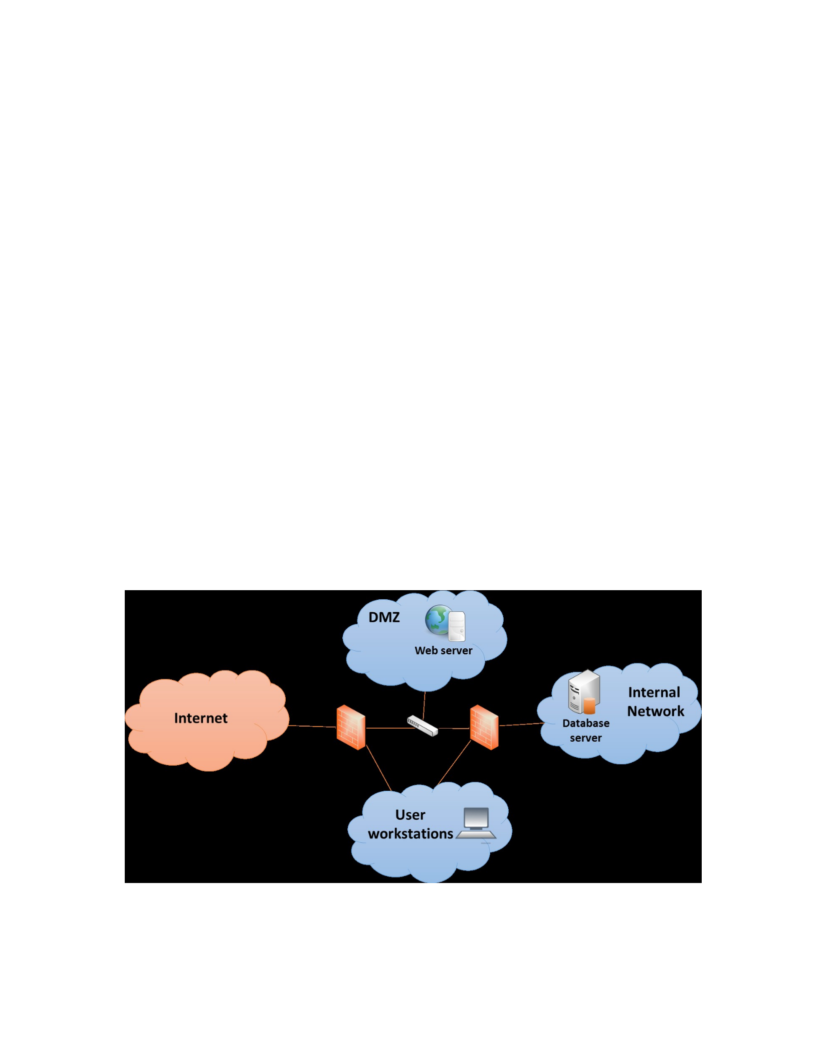
137
70% increases the number of new customers significantly and almost triples the daily website
traffic, leading to an increase in the organization's revenue.
The network topology for the organization is presented in Figure 29. This topology has
three network segments: Demilitarized Zone (DMZ), Internal Network, and User Workstations.
External and Internal Firewalls control access to Demilitarized Zone. DMZ is used for the
operations of the Web Server. Database Server is located in the Internal Network, which is
behind the Internal Firewall that has more strict firewall rules for access control. The user
workstations network is used by regular users.
Figure 29.
Network topology of the organization for the simulation

138
The following sections provide details on generating the impact graph for the simulations,
give the details about generating and analyzing the attack graph, provide the details of the
scenarios to be run on the simulation model, deliver the details of the impact graph analysis,
discuss the details of the simulation one by one for each scenario, and summarize the discussions
on the simulation results.
Generate the Impact Graph
A network with a similar impact graph to the one in Chapter 5 (Example) was selected for
the simulation for simplicity and clarification. Confidentiality, integrity, and availability (CIA)
weights, Strength of Dependency (SOD), and Criticality of Dependency (COD) values are
presented in Tables 18, 19, and 20, respectively. Since availability is relatively more important
for the website hosted by the organization, this can be indicated by the difference among the
weights of CIA components of the assets in Table 18. The impact propagation equations are
provided in Chapter 5 also apply to the simulation network. However, some of the inputs
(operability loss of nodes) and outputs (economic loss values) of the impact graph are different
since the attack graph is more complex than the one in Chapter 5. The workstations and users
(A7 – A10) are also included in the impact graph as different nodes; however, these nodes do not
have a dependency relationship with the other nodes (Figure 30). The effects of these assets are
observed only in the attack graph.
Figure 30.
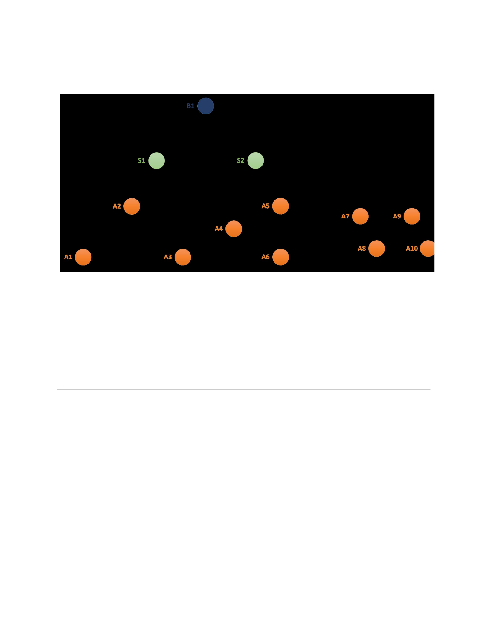
139
Impact graph for the simulation
Table 18.
CIA weights and descriptions of impact graph nodes
Node Name Type 𝒘𝒘𝑪
𝑪𝒊𝒊
𝒘𝒘𝑰
𝑰𝒊𝒊
𝒘𝒘𝑨
𝑨𝒊𝒊
Description
A1 External Firewall Asset 0.10 0.45 0.45 Filters traffic to the web
server.
A2 Web Server Asset 0.10 0.20 0.70 Hosts online course website
A3 Internal Firewall Asset 0.10 0.45 0.45
Filters traffic between the web
server and database server
A4 Database Server Asset 0.35 0.35 0.30
Archive of online course
videos and files.
A5 Web Application Asset 0.10 0.20 0.70
Provides students the ability to
enroll and pay for a course.

140
A6 Database Server Asset 0.35 0.35 0.30
Personal Identifiable
Information and financial
information of students.
S1 Web Hosting Service 0.20 0.30 0.50
Delivery of an up and running
website with online course
contents.
S2 Registration &
Billing
Service 0.35 0.35 0.30 Course registration and
payment of the fee by
students.
B1 Hosting a
Website
Business
Process
0.10 0.45 0.45 Delivering online education to
higher education students.
Table 18 and Table 19 provide the alpha and beta values between the dependency among CIA
aspects of constituent nodes where each row represents a feeder node while each column
stands for a receiver node. For example, 𝛼𝛼𝐴𝐴1𝐼𝐼,𝐴𝐴2𝐼𝐼 is 0.5 while 𝛽𝛽𝐴𝐴1𝐼𝐼,𝐴𝐴2𝐼𝐼 is 50. These
values are
assigned according to expert evaluation. A1 and A3 columns are empty since they are only feeder
nodes, i.e., not a receiver node. Similarly, B1 rows are empty since B1 is only a receiver node,
not a feeder node. The relationship between S2 and B1 is time-dependent and explained later.

141
Table 19.
Strength of dependency between feeder (rows) and receiver (columns) node pairs of the simulation model
A1C A1I
A1A A2C A2I A2A A3C
A3I A3A A4C A4I A4A A5C A5I A5A A6C A6I A6A S1C
S1I
S1A S2C
S2I
S2A B1C
B1I
B1A
A1C 0.5
A1I
0.5 0.5
0.5
A1A
0.5
A2C
1
A2I
1 1 1
A2A
1
A3C
0.5
0.5
A3I
0.5 0.5
0.5 0.5 0.5
0.5

142
A3A
0.5
0.5
A4C
0.5
A4I
0.5 0.5
0.5
A4A
0.5
A5C
1
A5I
1 1
1
A5A
1
Table 19. continued.
A1C A1I A1A A2C A2I A2A A3C A3I A3A A4C A4I A4A A5C A5I A5A A6C A6I A6A S1C
S1I
S1A S2C
S2I
S2A B1C
B1I
B1A
A6C 0.5
0.5 0.5
0.5

143
A6I
A6A
0.5
S1C
1
S1I
1 1 1
S1A
1
S2C
T
S2I
T T T
S2A
T
Table 20.
Criticality of dependency between feeder (rows) and receiver (columns) node pairs of the simulation
model

144
A1C A1I A1A A2C A2I A2A A3C A3I A3A A4C A4I A4A A5C A5I A5A A6C A6I A6A S1C
S1I
S1A
S2C
S2I
S2A B1C
B1I
B1A

145
A1C 50
A1I
50 50
50
A1A
50
A2C
100
A2I
100 100 100
A2A
100
A3C
50
50
A3I
50 50
50 50 50
50
A3A
50
50
A4C
50
50 50
50

146
A4I
A4A
50
A5C
100
A5I
100 100
100
A5A
100
Table 20. continued.
A1C A1I A1A A2C A2I A2A A3C A3I A3A A4C A4I A4A A5C A5I A5A A6C A6I A6A S1C
S1I
S1A S2C
S2I
S2A
B1C
B1I
B1A
A6C 50
A6I
50 50
50
A6A
50
S1C
100
100 100 100

147
S1I
S1A
100
S2C
100
S2I
100 100 100
S2A
100
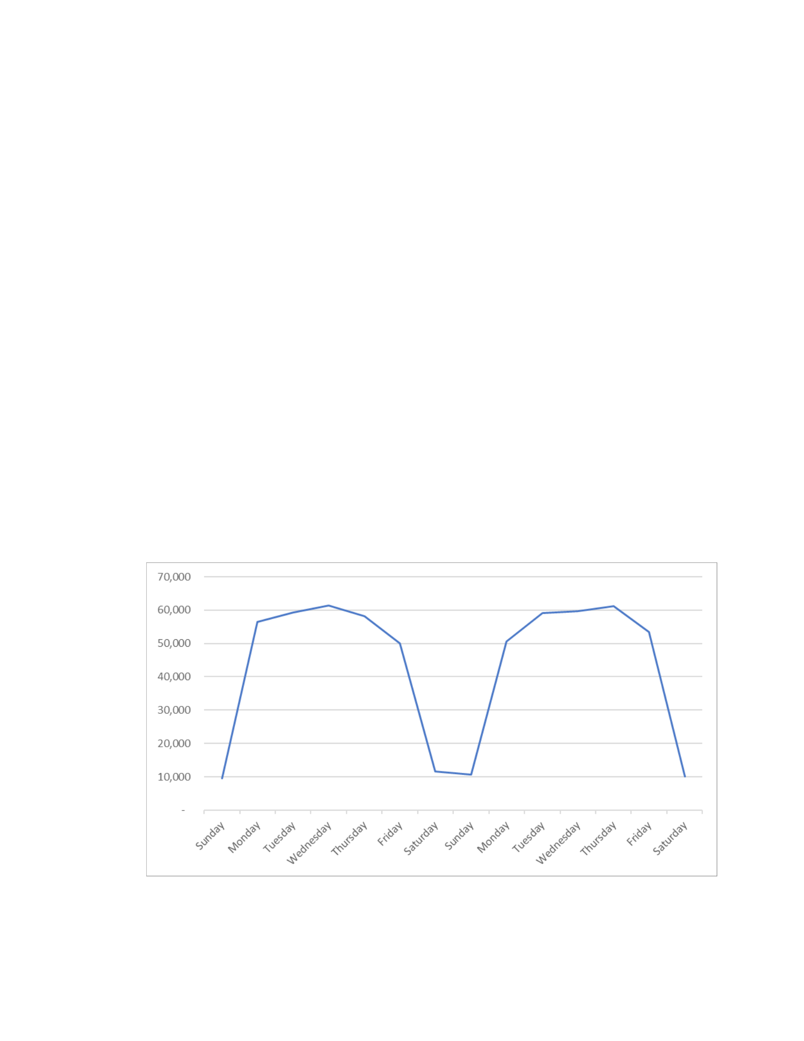
148
Time Unit Designation
The time unit designated for the study is one day (𝑖𝑖 = 𝑜𝑜𝑖𝑖𝐸𝐸). Time-dependent
variables such as the strength of dependency and cost items of the model are based on daily
values.
Time-Dependent and Probabilistic Variables
After the time unit is designated, the time-dependent variables should be estimated by the
decision-makers. For the estimates, historical data can be used, or expert judgment can be
elicited. For the simulation model, the regular daily traffic for the website is given in Figure 31
(Microsoft, 2019). Regular daily traffic is around 50-60 thousand clicks.
Figure 31.
Regular daily traffic for the website of the organization to be simulated

149
Time-Dependent Strength of Dependency. The Strength of Dependency relationship
between Service 2 (Registration and Billing) and Business Process 1 is time-dependent.
According to the hypothetical but realistic scenario, the decision-makers assume that during
routine operations, registration and billing service are used daily with a random number of 2 to
15 customers, while during promotion, it is a random number between 60 and 120. Since
randomly distributed uniform distribution is widely used in simulations, this distribution is
employed in the example. When the dependency of Business Process 1 to Service 2 is taken into
consideration, the Strength of Dependency parameter, alpha, receives a normally distributed
value with a mean of
0.1 and a standard deviation of 0.01 for routine operations. This means that for routine
operations, B1 is slightly dependent on S2. For the promotion period, the dependency increases,
and the mean parameter becomes 0.9, indicating that the new customer registration and billing
are crucial during the promotion. For the simulation, the specific values of the time-dependent
alpha parameter between S2 and B1 are randomly generated. Table 21 presents the relevant
distribution information and a random sample number for routine operations and the promotion
period.
Table 21.
Probabilistic alpha values for strength of dependency relationship between S2 and B1
Time Distribution α S2-B1 Random #
Routine U (2, 15) N (0.1, 0.01) 0.095068
Promotion U (60, 120) N (0.9, 0.01) 0.915118
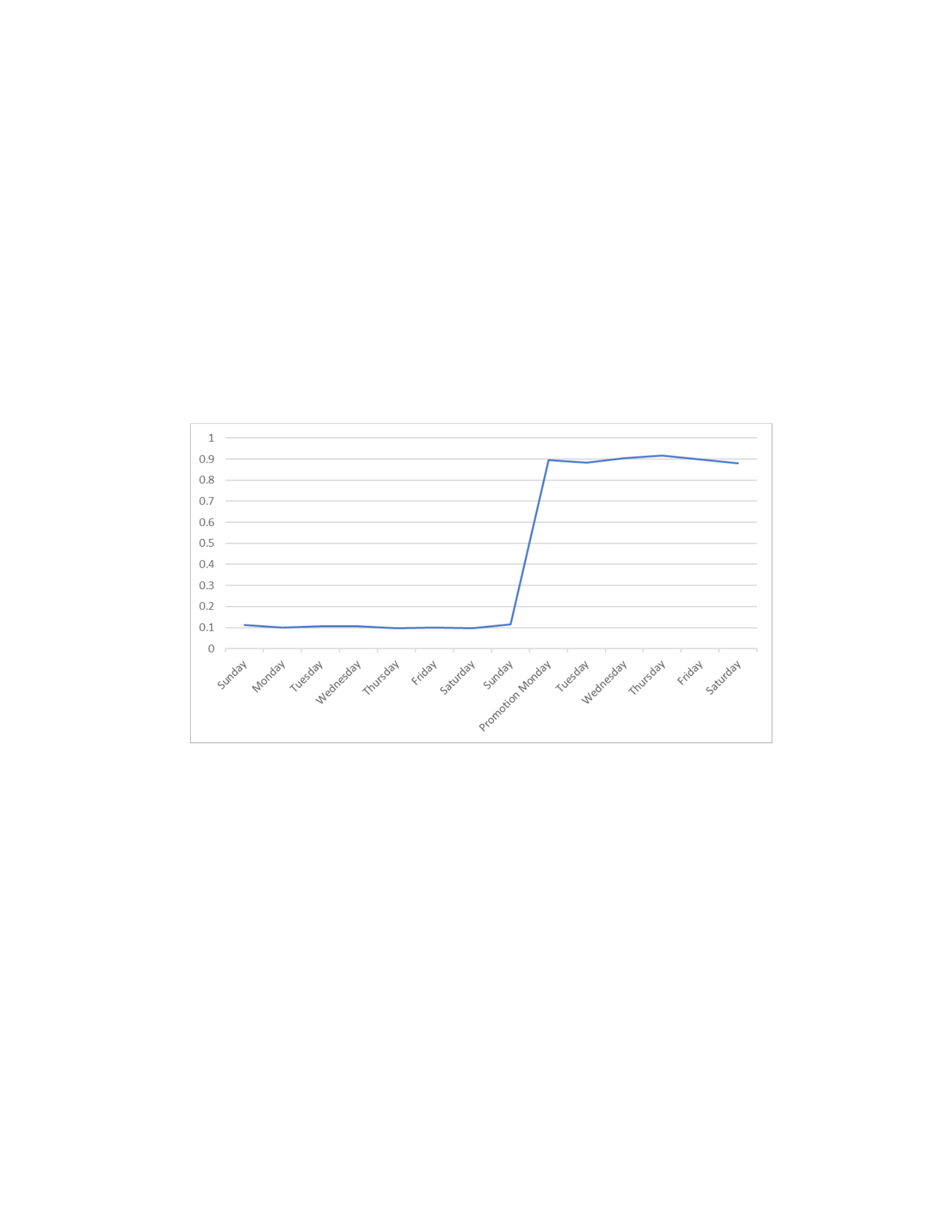
150
The randomly generated values of the time-dependent alpha parameter between S2 and
B1 for each day are presented in Figure 32. For the analysis, the relevant alpha value will be
employed for each iteration of the simulation.
Figure 32.
Randomly generated alpha values for the strength of dependency between S2 and B1
Time-Dependent Cost Items. For the simulation model, the regular daily traffic for the
website was given in Figure 31 (Microsoft, 2019). Regular daily traffic is around 50-60 thousand
clicks. The decision-makers estimate from the historical trends that during a promotion period,
the daily traffic almost triples. Figure 33 presents the estimated website traffic.
Figure 33.
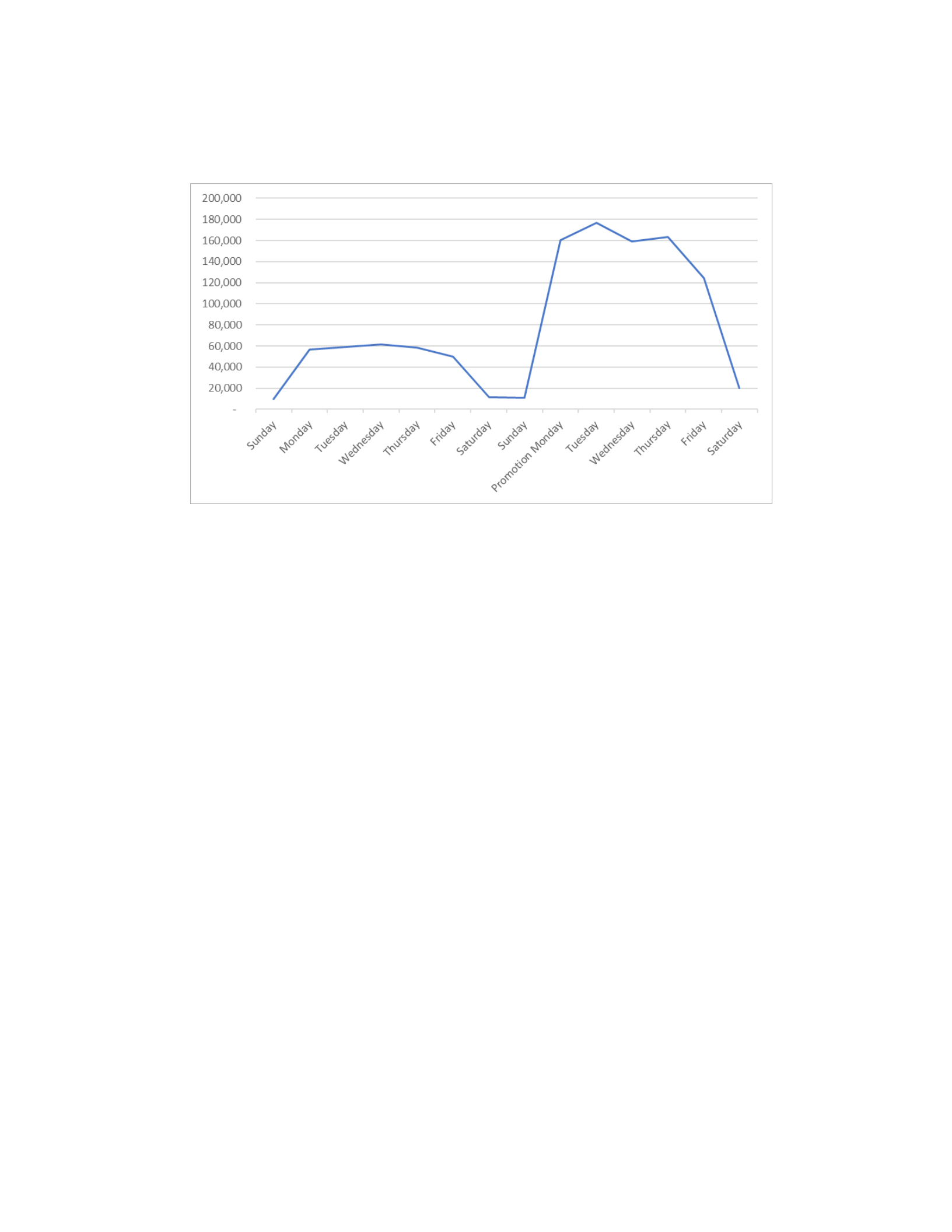
151
Estimated website traffic for before and during the promotion period
In order to calculate the time-dependent cost items such as Loss of Revenue and Loss of
Data and Equipment, the decision-makers should use historical data or expert opinion. Historical
revenue data, usage data, or any other relevant data can be helpful in this process. In this case
study, it is assumed that the daily traffic is directly affecting the revenue. By normalizing the
estimated daily web traffic data, the multiplier values for the time effect are determined. The
multiplier values are in a range from zero to one and determined for each day during the analysis
period (Figure 34).
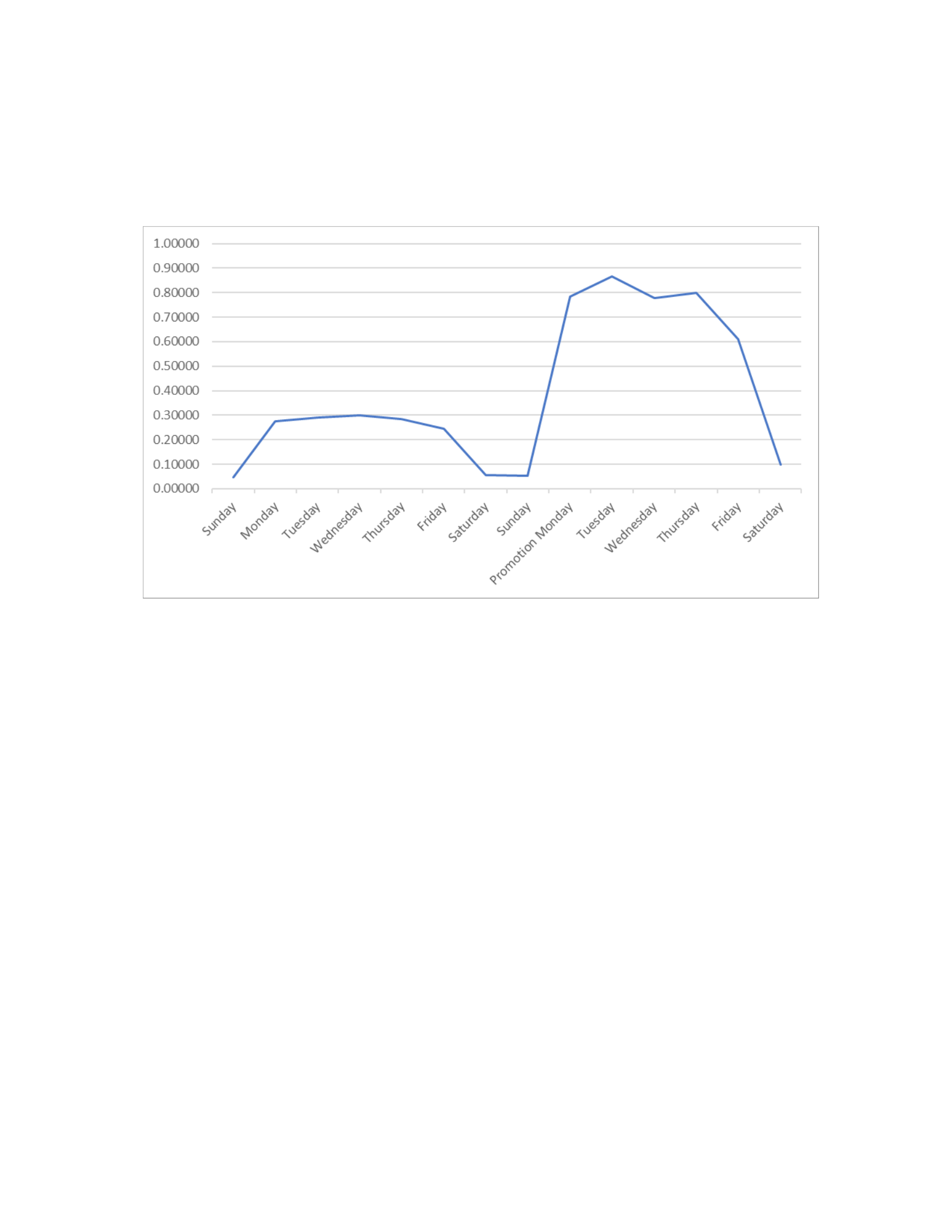
152
Figure 34.
The multiplier for time effect for before and during the promotion period
The multiplier values are used to calculate the daily values of Loss of Revenue and Loss
of Data and Equipment by multiplying with the estimated cost values. Since the multiplier values
are in a range that almost 0.3 represents the average value and almost 0.8 represents the higher
promotion values, 1 represents the expected maximum revenue. Therefore the cost estimates for
Loss of Revenue and Loss of Data and Equipment should be the highest expected values. Then,
for example, for an average day, it would be multiplied by a multiplier around 0.3. For the other
cost items, the estimates should be made as an expected average one-time cost. Based on this
concept, estimates for cost items are conducted and presented in Table 22. Its values are the same
as those in the example in Chapter 5; however, the simulation's time-dependent characteristics
differ from the example.

153
Table 22.
Cost estimates for the simulation
Loss of Data and Equipment 1 $ 19,565 $ 21,268 $ 17,081
Loss of Revenue 2 $ - $ - $ 234,358
Loss of Strategic Information 3 $ - $ - $ -
Reputational Damage 4 $ 3,622 $ 4,251 $ 4,648
Cybersecurity Improvements 5 $ 20,000 $ 30,000 $ 30,000
PR 6 $ 2,681 $ 2,923 $ 3,812
Regulatory Penalties 7 $ - $ - $ -
Court Settlement Fees 8 $ 5,000 $ 5,812 $ 5,000
Generate the Attack Graph
The attack graph for this network is presented in Figure 35. With the existence of
workstations and users within the topology, the attack graph grows, and new attack scenarios
(attack paths) emerge. A vulnerability exists on a web browser of a workstation that enables the
Cost Items Cost Item # C I A
Forensics 9 $ 4,162 $ 3,363 $ 5,503
Loss of IP 10 $ -
Increased Cost of Capital 11 $ -
Customer Protection 12 $ -
Breach Notifications 13 $ -
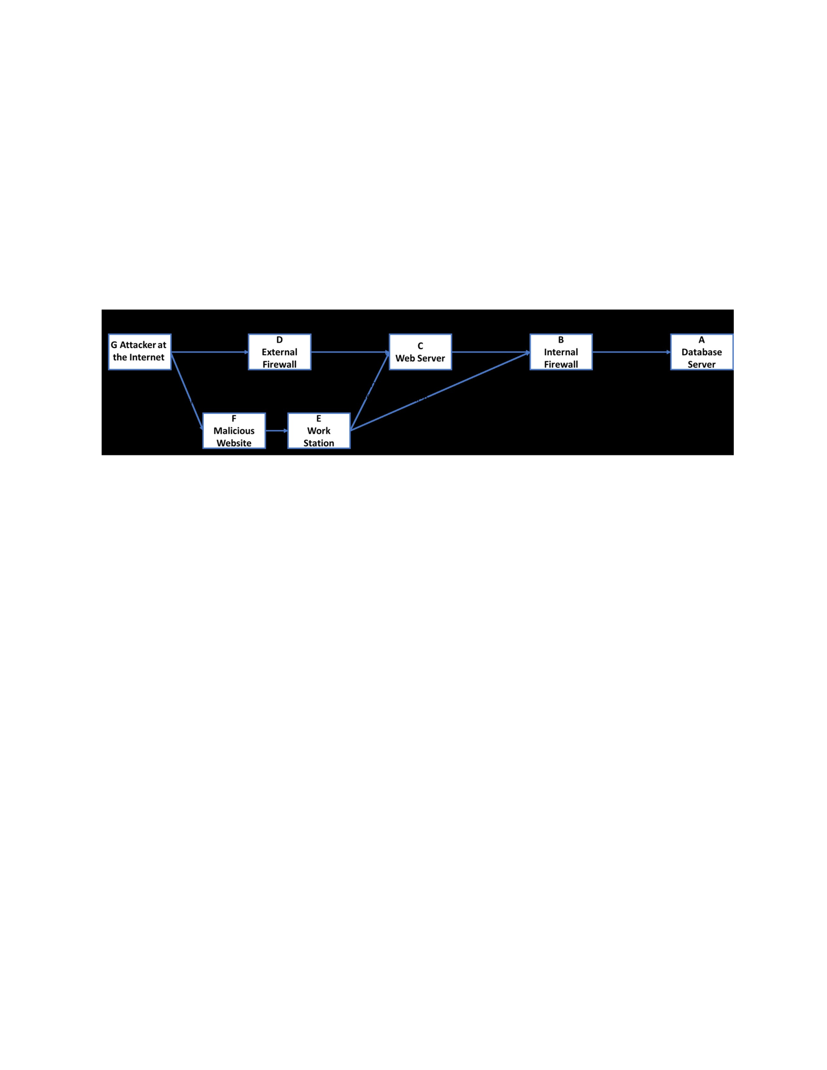
154
attacker to use a phishing e-mail to get a user to click on a link that leads to a malicious website
prepared by the attacker (Tatar et al., 2020).
Figure 35.
Attack graph for the simulation (Adapted from Singhal & Ou, 2011)
The attack graph for the simulation network includes three attack paths, which are
highlighted in Figure 36. The details of these three attack paths are as follows (Tatar et al., 2020):
1. G->D->C->B->A (Orange attack path): The attacker exploits vulnerabilities on the Web
Server and Database Server. This attack path is covered in the example in Chapter 5.
2. G->F->E->C->B->A (Green attack path): In this attack path, the attacker at the internet
prepares a phishing e-mail with a link that leads to malicious content if the user of the
workstation clicks on it. There are two steps of a phishing attack, preparing the phishing
content and getting a user to click on the link. After the workstation is compromised, the
attacker uses multi-hop access to reach the Web Server, then through the internal firewall
to the Database Server.
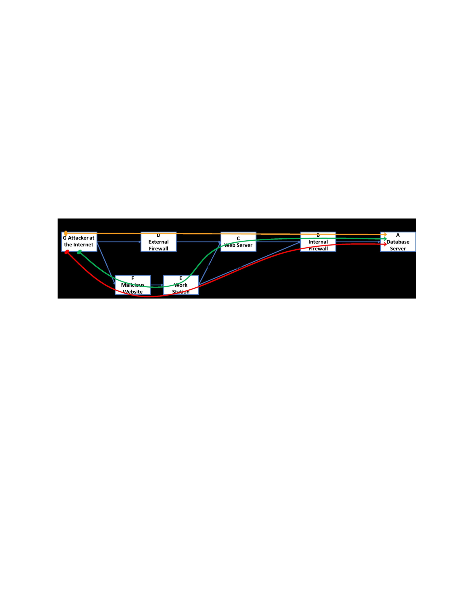
155
3. G->F->E->B->A (Red attack path): This attack path also includes phishing. The only
difference with the second path is that the attacker directly reaches the Database Server
from the workstation without accessing the Web Server.
Figure 36.
Attack graph with its three paths highlighted
Analyze the Attack Graph
In this attack graph, three vulnerabilities exist. CVE-2019-6111 and CVE-2019-18601
were provided in Chapter 5. The third vulnerability, CVE-2009-1918 (National Vulnerability
Database, 2019c), exists on the workstations. With this vulnerability, the Internet Explorer
browser installed on the workstations may allow attackers to execute arbitrary code via a crafted
HTML document that causes memory corruption. Detailed CVSS Values of CVE-2009-1918 in
the National Vulnerability Database are as follows (Tatar et al., 2020):

156
CVSS Values of CVE-2009-1918 on Workstation
Vector String: AV:N/AC:L/PR:N/UI:R/S:C/C:H/I:H/A:H
•Attack Vector (AV): Network
•Attack Complexity (AC): Low
•Privileges Required (PR): None
•User Interaction (UI): None
•Scope (S): Unchanged
•Confidentiality (C): None
•Integrity (I): None
•Availability (A): High
Numerical data in Table 23 is determined according to the information on NVD and Table
6. the unconditional probability is calculated using Equation 4 as 0.72.
Table 23.
Numerical values for vulnerability metrics for CVE-2009-1918
CVE-2009-1918
Metric Value Numerical Value
Attack Vector (AV) Network 0.85
Attack Complexity (AC) Low 0.77
Privileges Required (PR) None 0.85
User Interaction (UI) Required 0.62

157
Scope (S) Unchanged
Confidentiality (C) High 0
Integrity (I) High 0
Availability (A) High 0
Conditional Probability P(F|H) 0.7243
Multiple attack paths are analyzed to compute the Unconditional Probability values for
each node based on the equations provided by Wang et al. (2008) and Shetty et al. (2018). The
attack graph has three attack paths, and calculations for the unconditional probability values
consider all three attack paths. The calculations of unconditional variables are presented below
(Tatar et al., 2020).
𝑃𝑃(𝐴𝐴) = 0.5
𝑃𝑃(𝐼𝐼) = 𝑃𝑃(𝐼𝐼|𝐴𝐴) ∗ 𝑃𝑃(𝐴𝐴) = 0.724 ∗ 0.50 = 0.362
Where P(F|G) is the conditional probability related to the phishing attack.
𝑃𝑃(𝐸𝐸) = 𝑃𝑃(𝐸𝐸|𝐼𝐼) ∗ 𝑃𝑃(𝐼𝐼) = 1 ∗ 0.362 = 0.362
Where P(E|F) is the user’s susceptibility to an integrity attack (i.e., the probability of
clicking the phishing link) assumed to be one for this simulation, meaning that the user clicks the
link.
𝑃𝑃(𝑆𝑆) = 𝑃𝑃(𝑆𝑆|𝐴𝐴) ∗ 𝑃𝑃(𝐴𝐴) = 1 ∗ 0.50 = 0.50
P(C) and P(B) are calculated based on OR logic (Wang et al., 2008).
𝑃𝑃(𝐶𝐶) = 𝑃𝑃(𝐶𝐶|𝑆𝑆) ∗ 1 − 1 − 𝑃𝑃(𝐸𝐸)∗ 1 −𝑃𝑃(𝑆𝑆)

158
= 0.55 ∗ 1 − (1 − 0.362) ∗ (1 − 0.50) = 0.375
𝑃𝑃(𝐵𝐵) = 𝑃𝑃(𝐵𝐵|𝐸𝐸) ∗ 1 − 1 − 𝑃𝑃(𝐸𝐸)∗ 1 − 𝑃𝑃(𝐶𝐶)
= 1 ∗ 1 − (1 − 0.362) ∗ (1 − 0.375) = 0.601
𝑃𝑃(𝐴𝐴) = 𝑃𝑃(𝐴𝐴|𝐵𝐵) ∗ 𝑃𝑃(𝐵𝐵) = 0.993 ∗ 0.601 = 0.597
The summary of the unconditional probability values is presented in Table 24.
Table 24.
Summary outputs of attack graph analysis with unconditional probabilities
Asset Description Unconditional Probability Value
A5 Workstation P(E) 0.36
A1 External Firewall P(D) 0.50
A2 Web Server P(C) 0.38
A3 Internal Firewall P(B) 0.60
A4 Database Server P(A) 0.60
Developing Scenarios
The simulations consist of two cases within which the same set of scenarios exists.
•Case 1 compares a one-day cyber-attack that occurs on the week and weekend. The
comparison is made for an average week between:
o Thursday and o
Saturday.

159
•Case 2 compares a two-day cyber-attack that occurs before and during a promotion.
The comparison is made between: o Tuesday and Wednesday of an average week
(the first week) o Tuesday and Wednesday of a boosted week during
promotion (the second week).
Case 1: Comparison of a one-day cyber-attack that occurs on the week and weekend. Case
1 includes the following scenarios:

