


1
Chapter 1: Introduction
The modern era within the United States automotive industry has experienced tremendous
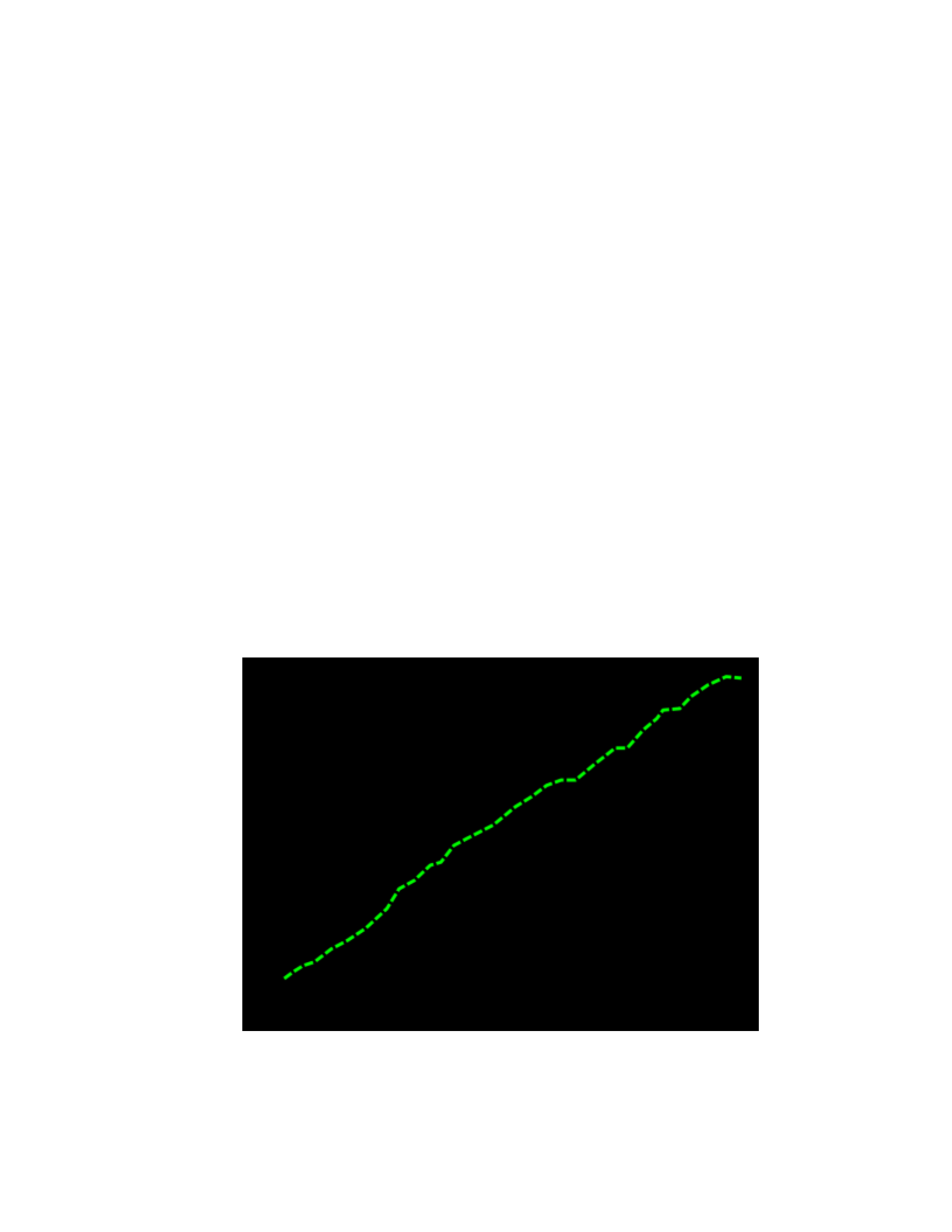
growth, with the number of registered motor vehicles increasing steadily by an estimated
3.69 million units annually from 1960 to 2008 [1]. Only in 2009, following the
automotive industry crisis, did the U.S. fleet decrease in size. Light vehicle sales in the
U.S. have rebounded since 2009; Ford Motor Company, Chrysler LLC and GM
experienced an overall sales increase of approximately 13.5% between 2012 and 2013
[2]. Furthermore, by the year 2020, global profits for automotive OEMs are expected to
increase by almost 50% [3]. Figure 1 illustrates the growth in the number of registered
motor vehicles from 1960 to 2009.

2
Figure 1: Growth in the number of U.S. Motor Vehicles [4]
From an environmental standpoint, this rapid growth presents a two-fold issue; an
increasing number of petroleum-consuming vehicles both diminishes already dwindling
oil supplies and invokes concern regarding the impacts of automotive exhaust byproducts
on the ecosystem. For these reasons, the EPA and NHTSA have enacted stringent fuel
economy and emissions policies on OEMs, with manufacturers who fail to achieve these
policies either forced to purchase surplus credits from other manufacturers or pay heavy
fines. Therefore, there is tremendous pressure on OEMs to look towards new and
innovative methods to improve fuel economy across their entire fleet. Figure 2 depicts the
United States CAFE compliance targets (in miles per gallon) for light-duty passenger
vehicles up to model year 2025. With the EIA estimating a 40.3 mpg fleet-wide average
for light-duty vehicles by model year 2021, it is clear that OEMs need to invest significant
research into reducing vehicle fuel consumption.
Projected Average Passenger Car CAFE Compliance Targets

3
Figure 2: CAFE Compliance Targets [5]
The effort to improve vehicle fuel economy and emissions quality without compromising
vehicle performance has resulted in an industry-wide push towards powertrain
optimization, with OEMs investing significant effort in a wide variety of fuel-reduction
technologies such as engine downsizing, cylinder deactivation, powertrain hybridization
and electrification, and flexible valve actuation. Improvements in vehicle fuel economy,
however, are not only limited to the benefits realized through optimizing engine
efficiency. As illustrated in Figure 3, coolant losses, exhaust energy losses, and the losses
associated with providing power to the ancillary loads all contribute to overall vehicle
fuel economy and therefore provide suitable grounds for vehicle efficiency
improvements.
Figure 3: EPA City/Highway Fuel Consumption [6]
The parasitic losses associated with the ancillary electrical loads, induced by the alternator
and transmitted through the auxiliary belt to the crankshaft, supply the electrical power

4
required for automotive necessities and appliances such as component actuation, lighting,
and infotainment systems. The management and control of these electrical loads, with the
objective of minimizing vehicle fuel consumption, has been largely neglected in years
past. However, as fuel economy mandates continue to challenge powertrain designers in
the coming years, the vehicle electrical system will become an increasingly attractive
reservoir of potential fuel savings.
The passenger vehicle electrical system has undergone dramatic changes throughout
history in order to compensate for ever-increasing vehicular load demands. What began as
a power system designed to satisfy in-cylinder ignition, cranking, and few (if any) lighting
loads has developed over time into a complex electrical system which supplies power to
various driver safety features, infotainment systems, control units, and electrical assist
systems. For example, the Volkswagen Golf, a typical passenger vehicle, experienced a
nearly 300% increase in the number of integrated ECUs from the 1998 to 2010 production
model [7]. Furthermore, it is predicted that by the model year 2020, dual-voltage
electrical systems composed of a 12/48V (nominal) battery pair will be commonplace
within the automotive industry [8]. This will allow for the electrification of loads once
mechanically coupled to the engine crankshaft, as well as the recuperation of the
automobile’s kinetic energy upon braking, improving overall vehicle fuel economy.
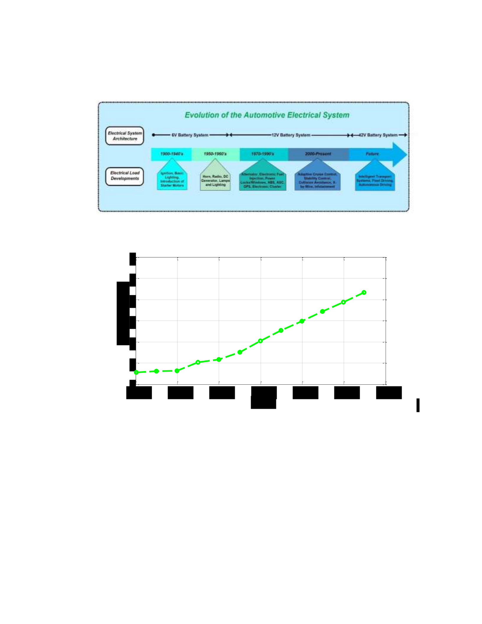
Figure 4 illustrates the evolution and predicted trajectory of the typical commercial
automotive electrical system, whereas Figure 5 demonstrates the increase in automotive
electric power demand over time. Given the incorporation of increasingly complex
5
electrical systems, one can easily imagine how quickly automotive electric power
requirements will grow in the future.
Figure 4: Evolution of the Automotive Electrical System [9].
Figure 5: Predicted Automotive Electric Power Requirements [10].
Figure 5 depicts one possible trajectory for automotive electrical power requirements up to
model year 2025, with power requirements predicted to more than double to
approximately 4.5kW (6 HP) between 2000 and 2025. The automotive electrical system is
inarguably responsible for a small, but increasingly significant percentage of overall
1970
1980
1990
2000
2010
2020
2030
0
1
2
3
4
5
6
Year

6
vehicle fuel consumption compared with years past, and the relevance of these electrical
systems can no longer be overlooked when optimizing for vehicle fuel economy. This,
coupled alongside increasingly stringent fuel consumption and emissions policies
enforced by the EPA (reference Figure 3), signifies that appreciable benefits may be
recognized through control optimization and management of the automotive electrical
system.
Section 1.1: Overview on the Role of Optimal Control Theory in the
Energy Optimization of Advanced Vehicles
One promising method of vehicle electrical system control and optimization lies in the
domain of optimal control theory. Optimal control theory, an extension of the wellknown
calculus of variations, allows for the control of the trajectory of a dynamic system in some
“best way”, as defined by the user (i.e. minimization of fuel consumption).
Optimal control theory’s origins may be traced all the way back to the 17th century, when
the calculus of variations was first developed [11]. However, it was not until the
development of the digital computer, first commercially available in the 1950’s, that
optimal control theory truly found widespread application. In more recent years, the rise
of the hybrid electric vehicle (HEV) has brought optimal control to the forefront of the
automotive industry. The potential benefits brought about by the management and
optimization of the various energy flows which accompany automotive hybridization
makes optimal control-based strategies an attractive field of study [12-14]. For instance;
dynamic programming (DP), while not implementable in real-time control systems, allows
7
one to easily observe the optimal “power-split” trajectory of an HEV, given that the
vehicle driving schedule is known a priori. This task is performed via a DP algorithm,
which examines all possible trajectories between two points and selects the most
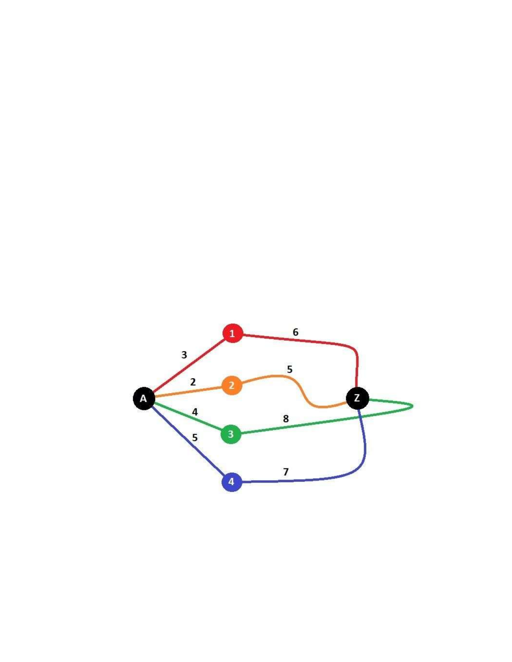
“optimal” solution. A very simple illustration of how dynamic programming functions
may be observed in the “shortest path” example featured in Figure 6. If the objective of
the dynamic programming sequence is minimization of the total distance travelled from
point A to point Z, then clearly path 2, with a net “distance” of 7 units, is the optimal
trajectory. This same logic may be expanded to very complex engineering problems,
however care should be taken as dynamic programming can become very computationally
expensive when analyzing particularly detailed systems.
Figure 6: Shortest Path Dynamic Programming Example.

8
Referencing [15], the advantages that dynamic programming present over a baseline
rulebased control strategy are significant, and upwards of an 18% reduction in fuel
consumption may be achieved over a single UDDS drive cycle. Dynamic programming
may therefore be utilized as a benchmarking tool to evaluate the efficacy of online,
suboptimal control strategies. In the same study, a control strategy termed the Equivalent
Consumption Minimization Strategy (ECMS), based off of Pontryagin’s Minimum
Principle, yields fuel savings of approximately 12%. The ECMS control strategy
effectively weights usage of the chemical energy stored within the automotive battery
against the consumption of fuel by the internal combustion engine in order to determine
the optimal power split and, similar to dynamic programming, cannot be implemented into
real-time control without some adaptions being made first. The development of an
adaptive-ECMS controller, implementable in real-time, utilizes feedback from the battery
state of charge to realize fuel savings only 1-2% lower than that of an ideally tuned ECMS
model [16]. In a study performed at OSU, a control strategy utilizing
Pontryagin’s Minimum Principle demonstrates the flexibility of optimal control theory,
minimizing cumulative PHEV tailpipe and corresponding power-plant carbon dioxide
emissions in place of fuel consumption [17].
The benefits of optimal control within the automotive sector certainly are not limited to
applications involving hybrid electric vehicles. Conventional powertrain automobiles
with a standard, 12V charging system exhibit significant improvements in fuel economy
when subjected to implementable control. Research indicates that quadratic programming

9
has been successfully applied to the electrical system of a conventional powertrain
automobile, leading to experimental fuel economy improvements of up to 2.6% on a Ford
Mondeo [18]. In a separate study performed at The Ohio State
University’s Center for Automotive Research, the efficacy of the well-known ECMS
control strategy is evaluated side-by-side, in simulation, with a standard commercial
control scheme, demonstrating fuel economy improvements of up to 1.5% on a vehicle
[19].
The rapid rise of information and communication technology, particularly developments in
Vehicle-to-Vehicle and Vehicle-to-Infrastructure communication, has allowed for a very
promising application of optimal control; intelligent transportation systems (ITS). By
enabling inter-vehicle communication, large, densely-packed arrangements of automobiles
(termed “platoons”) may be formed. These tight formations ideally reduce the cumulative
aerodynamic drag on the platoon, improving fuel economy while cutting down on
roadway congestion. One particular study even points towards fuel savings ranging from
5-15% in an optimal control, heavy-truck platooning application [20].
Figure 7 illustrates the general concept of platooning and intelligent transport systems.

10
Figure 7: Intelligent Transport Systems, Platooning Scenario [Volvo].
The benefits of optimal control in the ITS industry go beyond improving vehicle fuel
economy; by allowing automobiles to access information regarding surrounding road
conditions, the optimal vehicle trajectory with respect to net time travelled may be
developed and adapted in real time. This not only improves driver comfort, but also
provides a partial solution to the issue of increasingly crowded metropolitan transportation
systems. As ITS-enabling technologies gain a foothold in the United States and become
commonplace in the automotive sector, significant research effort will likely be dedicated
towards the study of automotive platooning and fleet management optimal control.
With the advent of the digital age in the 1950’s, optimal control theory has become an
increasingly valuable tool to engineers. The adaptability of optimal control theory allows
for widespread application in the automotive sector, from determining the most
timeeffective path to an end destination, to minimizing an individual vehicle’s fuel
consumption and exhaust emissions, and even utilizing Intelligent Transport System data
to reduce net time spent in traffic and maximize fleet fuel economy. As consumer

11
dependence on automotive electronics continues to grow and CAFE regulations stress
OEMs to look to new and innovative methods of reducing fuel consumption, the
integration of optimal control-based strategies will prove a cost-effective solution.
Section 1.2: Scope of Work
The Ohio State University’s Center for Automotive Research (OSU-CAR) is working in
conjunction with Chrysler Group LLC and the U.S. Department of Energy in order to
develop advanced powertrain technologies which demonstrate an overall fuel economy
improvement, on a Vehicle, of 25% over the Federal Test Procedure drive cycle. As part
of the team dedicated to this effort, OSU-CAR is responsible for the development of a
supervisory vehicle energy control strategy for vehicle ancillary loads which should
improve fuel economy through an improved coordination of the main vehicle energy
consumers. These improvements are recognized through the management and reduction
of the ancillary loads, as well as the management of the vehicle thermal system. The
focus of this document is on the development and implementation of an ancillary load
reduction (ALR) control strategy.
Section 1.3: Document Layout
The remainder of this thesis is structured as follows:
• Chapter 2 first describes the various experimental setups used to develop the
comprehensive Vehicle Electrical System (VES) model. An in-depth discussion
regarding the numerous designs of experiments used to develop the model is then

12
laid out. The structure of the VES model is discussed from a component level,
followed by validation of the VES model.
• Chapter 3 begins with a general discussion regarding the VES optimal control
problem. An in-depth analysis of a single VES optimal control scenario is then
performed. The robustness of the control strategy is then investigated through
various sensitivity analyses. Finally, this analysis is expanded to numerous
scenarios, and the overall behavior of the optimal control strategy is characterized.
• Chapter 4 discusses, in effect, how the gap was bridged between a
nonimplementable optimal control strategy and a real-time capable VES controller.
The adaptations made to the optimal control strategy in order to realize an online
controller are first discussed. The impact of these adaptations on both plant behavior
and fuel economy are then investigated. Finally, the experimental improvement in
vehicle fuel economy for the Chrysler Town & Country over numerous drive cycles is
presented.
• Chapter 5 concludes the work performed on the Ancillary Load Reduction (ALR)
project, highlighting the critical findings of the study and indicating potential
directions for future work.

13
Chapter 2: Model Development, Calibration, and Validation
The development, design, and integration of a control strategy is typically an iterative
process, which requires the designer to build, calibrate, test and modify new designs. The
use of physics-based or empirically-derived system models are essential to this process,
allowing the designer to perform several tasks in an accelerated environment with little to
no hardware in hand. When considering a complex, multi-domain system, for instance the
electrical infrastructure of a conventional automobile, the advantages that a system model
presents become quite evident. The lengthy process of designing an experimental setup,
testing a control algorithm, performing data acquisition, and post-processing may be

14
significantly expedited, with time instead spent on control design improvements. For this
reason, a Vehicle Electrical System (VES) model has been developed to facilitate in the
energy analysis of an automotive electrical system and control algorithm development.
This chapter first outlines the various experimental setups employed for the calibration
and validation of the VES model. A brief overview of the vehicle fuel consumption model
is then presented, followed by a more in-depth discussion regarding the development and
validation of the vehicle electrical system model.
Section 2.1: Experimental Setup Overview
A reliable and robust design of experiment is required to ensure that a simulation model
provides realistic and accurate results, a basic requirement for any energy management
supervisory control. Numerous experimental setups are utilized for this purpose. The use
of a chassis dynamometer, a 2011 Vehicle, and ETAS rapid prototyping equipment were
employed to allow for the development and validation of the VES model, as well as for
the proceeding implementation of the energy management control strategy. In addition,
the development of the battery model required a separate experimental set-up, consisting
of an environmental chamber and a programmable load/supply system.

15
2.1.1: Description of the Test Vehicle Setup
A 2011 Chrysler Town and Country minivan was available for testing at The Ohio State
University Center for Automotive Research (OSU-CAR). The main vehicle specifications
are given in Table 1 below.
Table 1: Vehicle Specifications
Make, Model, and Year
Chysler Town & Country, 2011
Engine
DOHC 24-valve V-6, 3604 cc
Transmission
62TE 6-Speed Automatic
Gear Ratio:1
4.127 – 2.842 – 2.284 – 1.452 – 1.0 – 0.69
Axle Ratio
3.16
Mass (kg)
2154
Frontal Area (𝐦𝟐)
2.42
0.33
Drag Coefficient (𝐂𝐝)
The test vehicle was installed on a light-duty chassis dynamometer available at CAR with
real-time driver feedback monitoring and recording live data from the vehicle. This setup
allowed for a level of experimental repeatability that may otherwise be difficult to
achieve. The use of a chassis dynamometer, as opposed to an engine dynamometer, also
allows one to observe the complex, multi-domain (electro-mechanical) dynamics that exist
within modern-day automobiles. Take, for example, the interactions between an engine,
the vehicle electrical system, and the numerous peripheral devices that are driven by the
auxiliary belt. By utilizing a chassis dynamometer, the effects of the various electrical
loads may be investigated, whereas with an engine dynamometer these effects are
typically ignored. The light-duty chassis dynamometer at The Center for Automotive

16
Research is equipped with two 24” rollers and is capable of handling up to 150 HP. A
Labview VI containing both the vehicle velocity profile and the desired vehicle speed
trace (if any) is displayed on a monitor to facilitate the driver in reproducing regulatory or
custom-made drive cycles. Figure 8 depicts the experimental chassis dynamometer setup,
complete with the drivers-aid display and the 2011 Vehicle.
Figure 8: Overview of the Test Vehicle and Light-Duty Chassis Dynamometer at
CAR.

17
2.1.2: Description of the Vehicle Electrical System Test Setup
Real-time measurement and data acquisition of the various dynamic variables and states
that exist within the vehicle’s electrical system is of the utmost importance in the
development of the Vehicle Electrical System model and validation of the vehicle energy
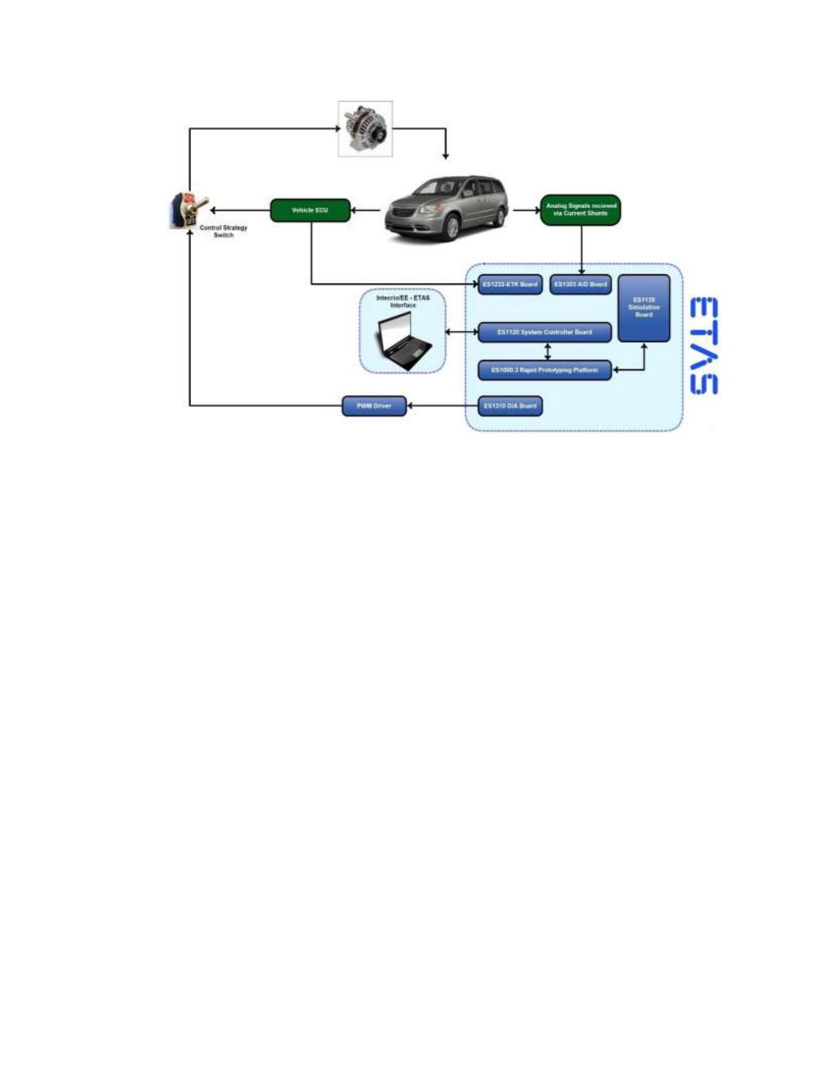
supervisory control strategy. An ETAS ES1000.3 rapid prototyping platform coupled with
Intecrio software allows for data acquisition and control testing. Shunts routed to an
ES1303 A/D board allow for measurement of the battery current, alternator current, and
cumulative electrical load demand, while an ETAS ETK-ECU interface gives direct access
to the control variables and parameters of the vehicle ECU. In addition to the data
acquisition setup, an ETAS ES1310 D/A board in conjunction with a PWM driver allows
for the override of the production control strategy for the vehicle alternator. This feature
allows one to implement and test control algorithms for the electrical system, as discussed
in Chapter 4. Finally, a programmable load was also required for fully characterizing the
vehicle electrical system, simulating the impact of auxiliary electrical loads in a
controllable and repeatable fashion. The use of a chassis dynamometer, ETAS rapid
prototyping and data acquisition platform, and the programmable load/supply allows for a
full characterization of the vehicle electrical system. A simplified schematic of this
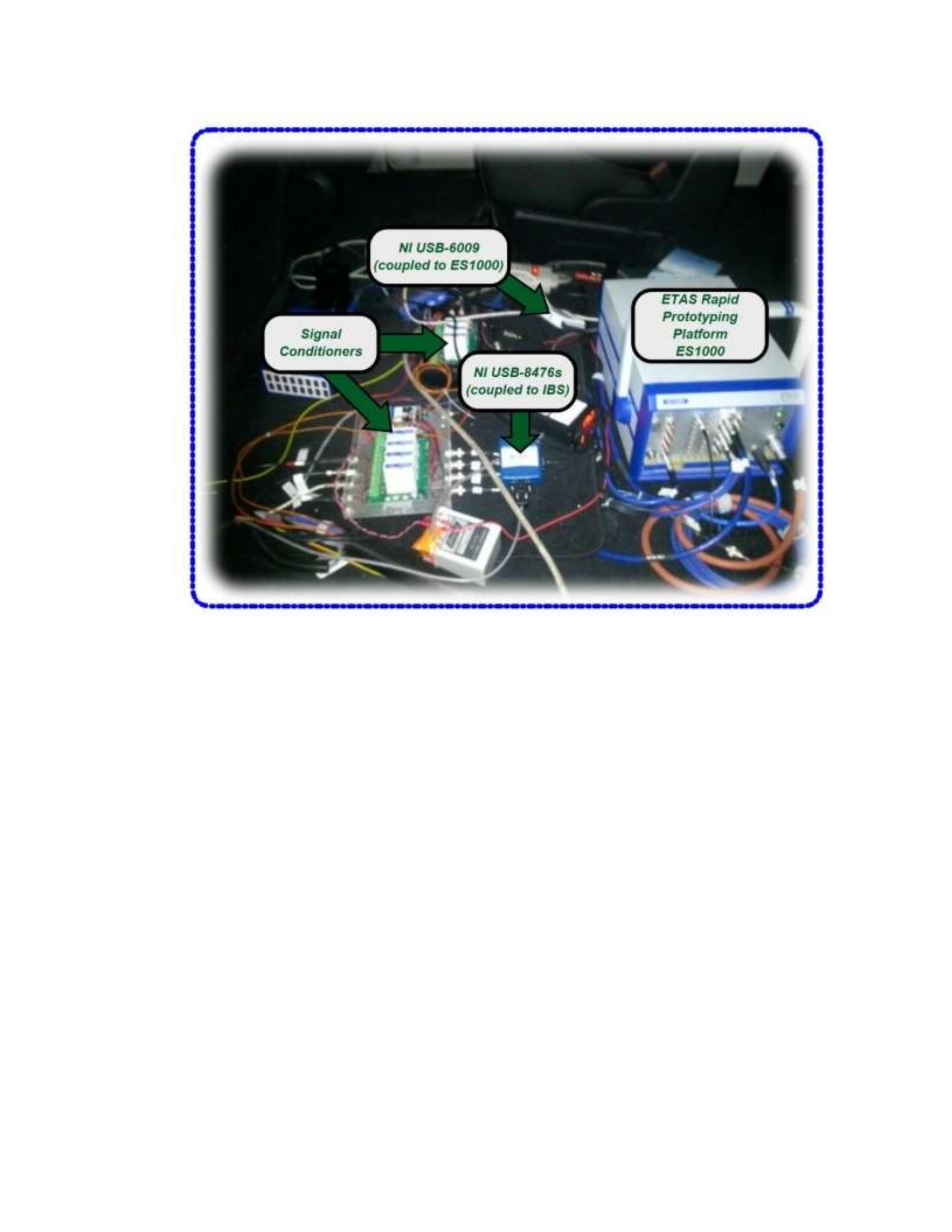
experimental setup is featured in Figure 9. The physical setup of the ETAS system, in the
backseat area of the minivan, is pictured in Figure 10.
18
Figure 9: Schematic of the Vehicle Electrical System Test Setup.
19
Figure 10: ETAS Experimental Setup
2.1.3: Description of the Battery Testing Experimental Setup
A standalone experimental setup for the battery present in the Chrysler vehicle allows for
one to conduct tests in a more controlled environment than what is possible with a test
vehicle. Battery parameter calibration and model validation are more easily performed on
a standalone battery setup due to the ability to accurately control the input current profile
and the thermal boundary conditions. Table 2, featured below, summarizes the main
specifications of the VES battery.

20
Table 2: Automotive Battery Specifications
Type
Lead-Acid, Flooded
Nominal Voltage (V)
12
Nominal Capacity (Ah)
75
Maximum Charging Current (A)
120
In order to control the electrical loads on the battery, determine the temperaturedependent
battery model parameters, and facilitate the deployment of the numerous experiments
required to fully characterize a battery model, a Testequity Model 140 environmental
chamber and a Maccor Series 4000 programmable load/supply are utilized. The Maccor
battery cycler allows for the user to define current profiles, such as constant current –
constant voltage (CC-CV) charge/discharge profiles or custom-made current profiles,
integrate looped combinations of these profiles, and record the resultant current and
voltage traces to a test computer for data post-processing. These tests may be repeated at
numerous set temperatures through the use of the environmental chamber.
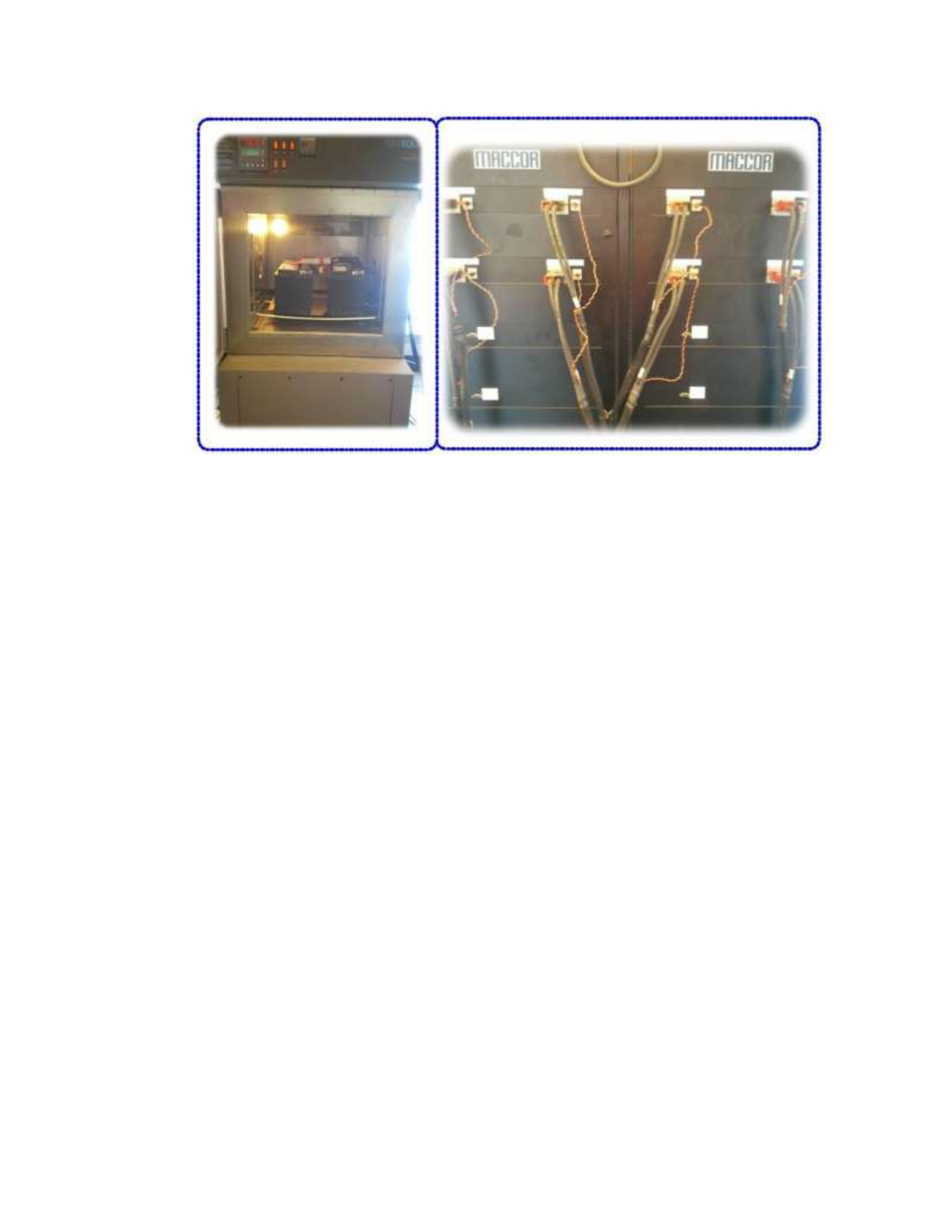
Figure 11 depicts this experimental setup.
21
Figure 11: Experimental Setup for Battery Testing (Left: Environmental Chamber
with Instrumented Batteries; Right: Maccor Battery Cycler).
Section 2.2: Overview of the Engine Fuel Consumption Model
The development of an accurate engine fuel consumption map is crucial to evaluating the
impact of a vehicle energy supervisory control strategy on fuel economy. To this extent,
Chrysler provided a set of engine experimental data (termed “Big Grid”) consisting of 247
steady-state engine speed and torque combinations. For each engine operating point, a
complete set of variables characterizing the breathing, fuel injection, combustion, torque
generation and emissions performance of the engine was available. From the given
experimental data, a simple fuel consumption map was built as a function of the engine
speed and torque inputs. This model is purely algebraic, and therefore does not take into
account any dynamic effects on the engine fuel consumption. While this approximation
would be inaccurate for the simulation of the engine dynamics, it is compatible with the
22
purpose of evaluating vehicle fuel consumption over extended periods of time, such as
drive cycles. In this case, the breathing and fuel dynamics of the engine, which affect the
fast dynamics of the engine torque output, are negligible, allowing for a static fuel
consumption model to be considered sufficiently accurate.
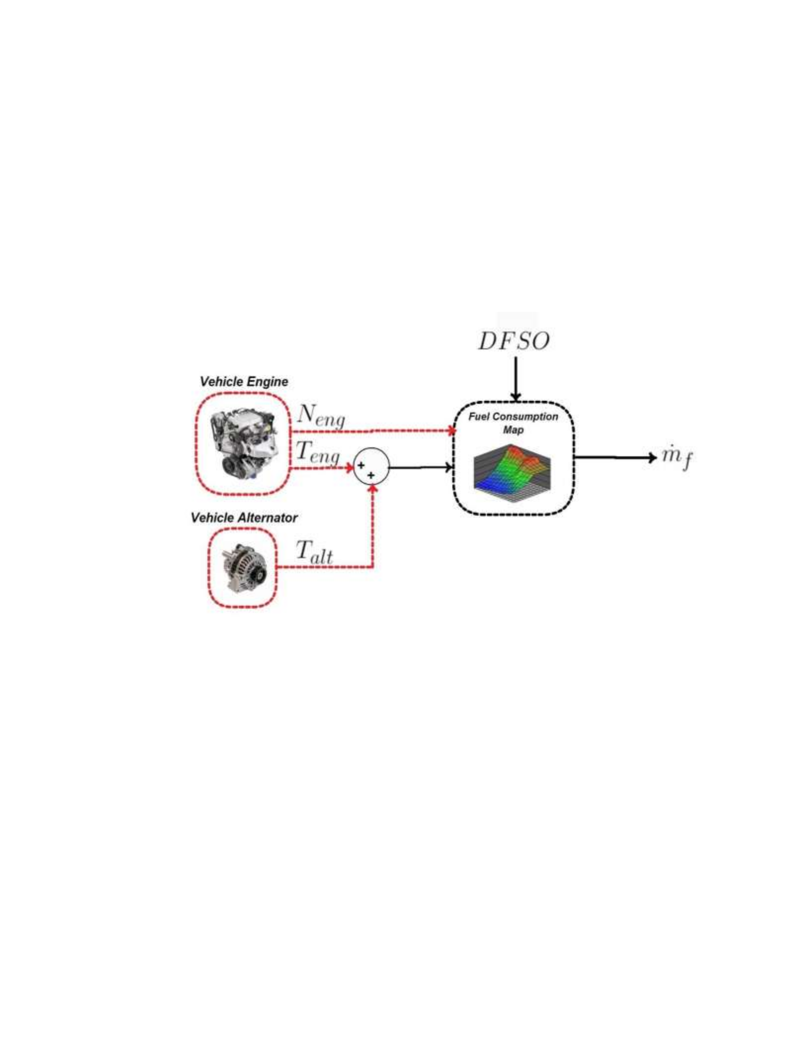
Figure 12 depicts the block diagram of the fuel consumption model.
Figure 12: Block Diagram of the Engine Fuel Consumption Model.
The fuel consumption model takes both the engine speed and the sum of the engine and
alternator torques as inputs, and outputs the fuel mass flow-rate. This allows one to
quantify the impact of the alternator power consumption on the vehicle fuel economy once
the engine fuel consumption model is integrated into the Vehicle Electrical System model.
The additional input, termed DFSO, accounts for the engine deceleration fuel shut off, and

23
sets the instantaneous fuel consumption to zero when active. A linear curve-fitting
approach is utilized as the method of interpolation to interpolate the experimental fuel
consumption and populate the map. Figure 13 depicts the fuel consumption data points
and resulting fitted lines.
Figure 13: Linear Fit of Fuel Mass Flow Rate.
Section 2.3: Description of the Vehicle Electrical System Model
A model of the Chrysler Town and Country’s electrical system is necessary for the
successful design of an energy management control strategy. In order to develop the
vehicle electrical system model, three subsystem models, namely the alternator, battery
and Chrysler controller (termed “Electronic-Voltage Regulator, or “EVR”), are developed
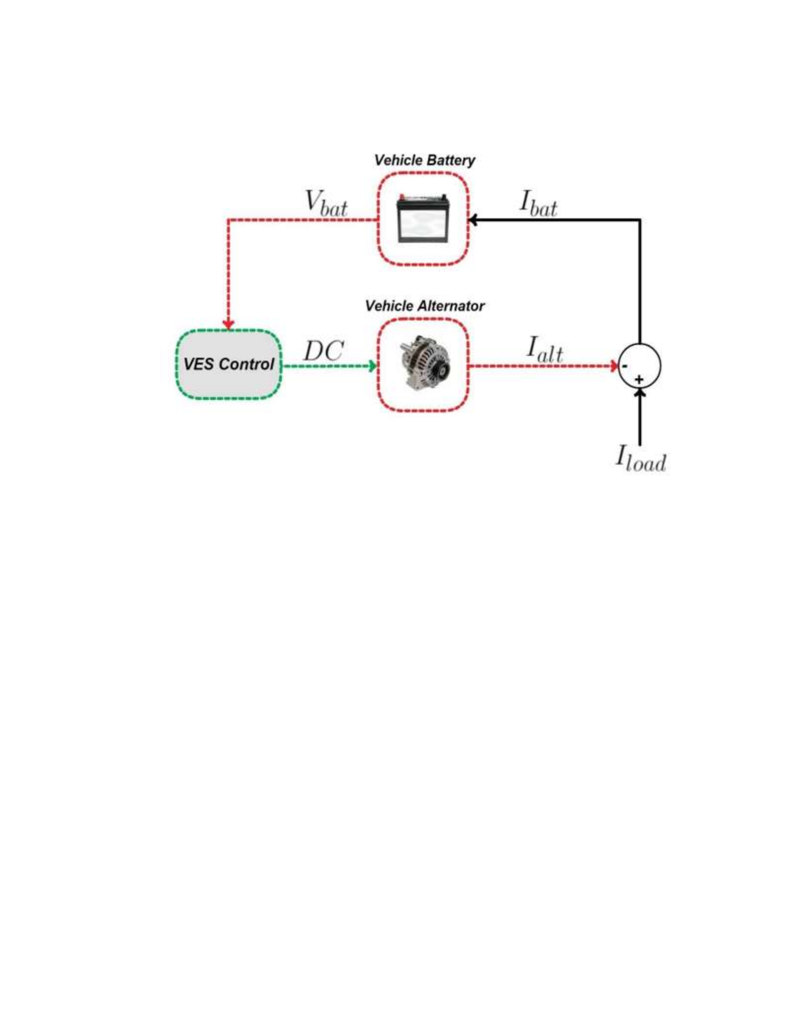
and independently validated. Figure 14 presents a block diagram showing the cause and
effect relationships of the three interconnected models.
24
Figure 14: Block Diagram of the Vehicle Electrical System Model.
The Electronic-Voltage Regulator is a model that mimics the production control strategy
for the electrical system. The algorithm monitors the battery voltage and outputs the
appropriate duty-cycle (DC) PWM signal to the alternator with the objective of
maintaining a nominal, temperature-dependent reference battery voltage. The duty-cycle
command results in an increase in the alternator field current, thus increasing the
alternator output current. The difference between the electrical load demand and the
alternator current is the current directed to the battery. The alternator, battery, and EVR
model will all be described in greater depth in the following sections, followed by an
analysis of the entire vehicle electrical system model.

25
2.3.1: Alternator Model
Numerous methods are available to model the input-output response of an automotive
alternator, ranging from the more complex and calibration-intensive circuit models to the
simpler, empirically-derived “black-box” models. [21] discusses the development of an
alternator circuit model in great detail. This type of approach is useful in capturing the
high-frequency dynamics of the electric generator and the switching behavior of the
AC/DC converter, and is typically used for electrical system fault diagnosis or
actuatorlevel control design. In this work, an experimentally-derived, map-based
alternator model will be integrated into the vehicle electrical system model. Maps
provided by
Chrysler for both the alternator torque and alternator efficiency were supplemented by
OSU-generated maps for the field current and the resultant alternator current. The general
form of these four look-up tables is described in Equations 1, 2, 3 and 4 below, followed
by Figure 15 which features contour plots depicting each output variable for a fixed
battery voltage:
𝑇𝑎𝑙𝑡 = 𝑇𝑎𝑙𝑡(𝜔𝑎𝑙𝑡, 𝐼𝑓, 𝑉𝑏𝑎𝑡)
(1)
𝜂𝑎𝑙𝑡 = 𝜂𝑎𝑙𝑡(𝜔𝑎𝑙𝑡, 𝐼𝑓, 𝑉𝑏𝑎𝑡)
(2)
𝐼𝑎𝑙𝑡 = 𝐼𝑎𝑙𝑡(𝜔𝑎𝑙𝑡, 𝐷𝐶, 𝑉𝑏𝑎𝑡)
(3)
𝐼𝑓 = 𝐼𝑓(𝜔𝑎𝑙𝑡, 𝐷𝐶, 𝑉𝑏𝑎𝑡)
(4)

26
Alternator Speed [RPM] 0 0 Duty Cycle [%] Alternator Speed [RPM] 0 0 Duty Cycle [%]
Figure 15: Alternator Contour Plots for a Fixed Battery Voltage.
The field current and alternator current maps, both considered functions of the alternator
duty-cycle, rotor speed, and battery voltage, are developed with the assistance of the
vehicle experimental setup (reference Section 2.1.3). The light-duty chassis
dynamometer, a vehicle modified with shunts to monitor the alternator and field currents,
a programmable load to fix the battery voltage, and a PWM driver which controls the duty
cycle are utilized for this purpose. With all three model inputs fully controlled, steady-
state data is then extracted via an ETAS ES1000.3 rapid prototyping platform, post-
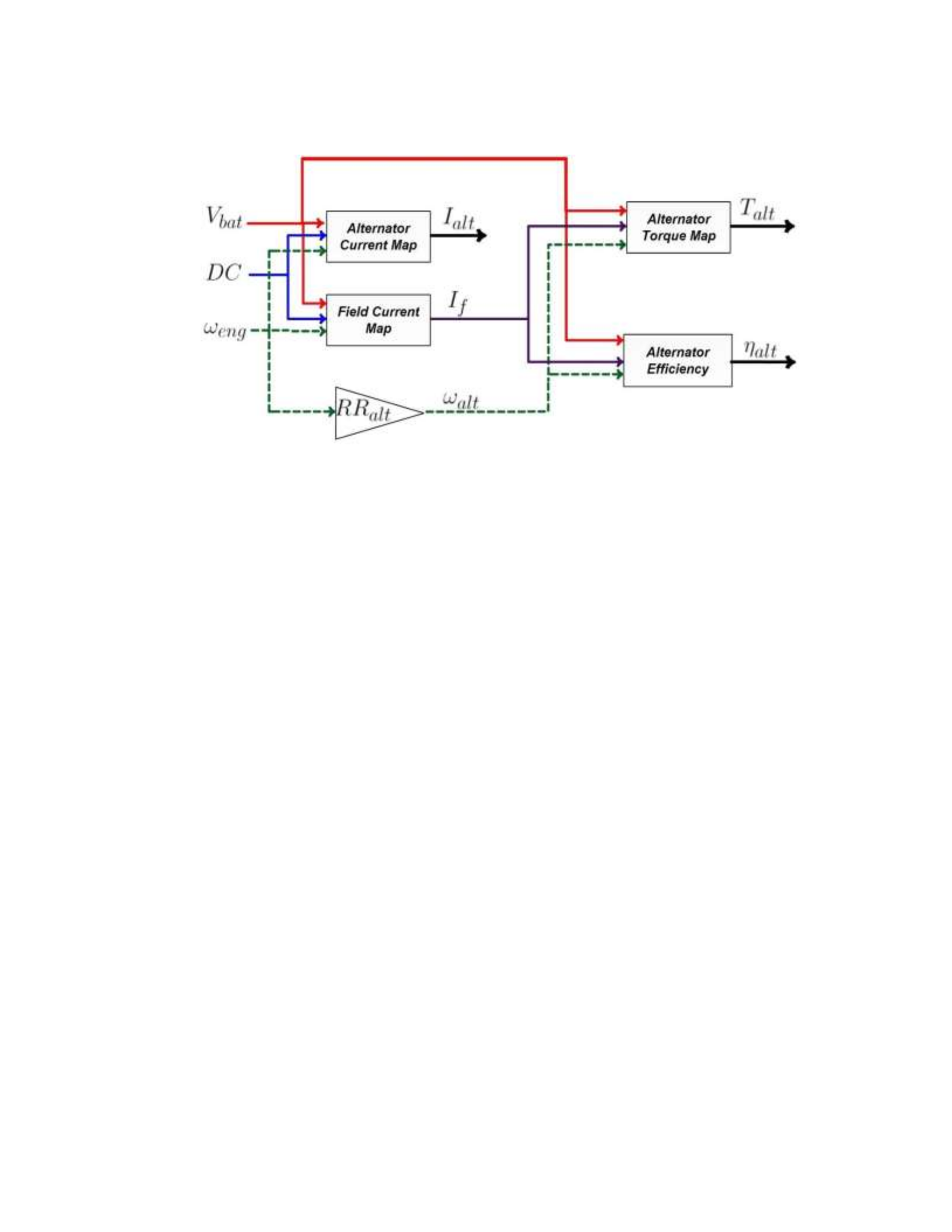
processed, and incorporated into the corresponding look-up tables. The block diagram
depicting the alternator model may be observed in Figure 16. Take note that 𝑅𝑅𝑎𝑙𝑡 is the
reduction ratio across the engine crank and alternator pulleys.
27
Figure 16: Block Diagram of the Alternator Model.
2.3.2: Battery Model
Modeling the voltage response of lead-acid batteries is a well-known process, which has
been approached by many researchers in the past [22-24]. In this context, several
modeling approaches have been proposed, depending upon the particular requirements
and the objectives of the model. For instance, electrochemical lead-acid battery models
have been developed to predict the very complex thermal and chemical interactions
between the electrodes and electrolyte [24]. Such models, while useful to explain the
voltage output behavior from first principles, are often too complex for integration into an
electrical system model for control development. On the other hand, equivalent electrical
circuit models offer a trade-off between accuracy and complexity that favors the
application of model-based control. These models typically relinquish a certain degree of
accuracy and physical consistency in exchange for increased simplicity. Despite the
28
simplistic nature of such a model, the overall input-output behavior of a battery may be
captured for a variety of operating conditions assuming that proper calibration of all
parameters is performed [22, 23].
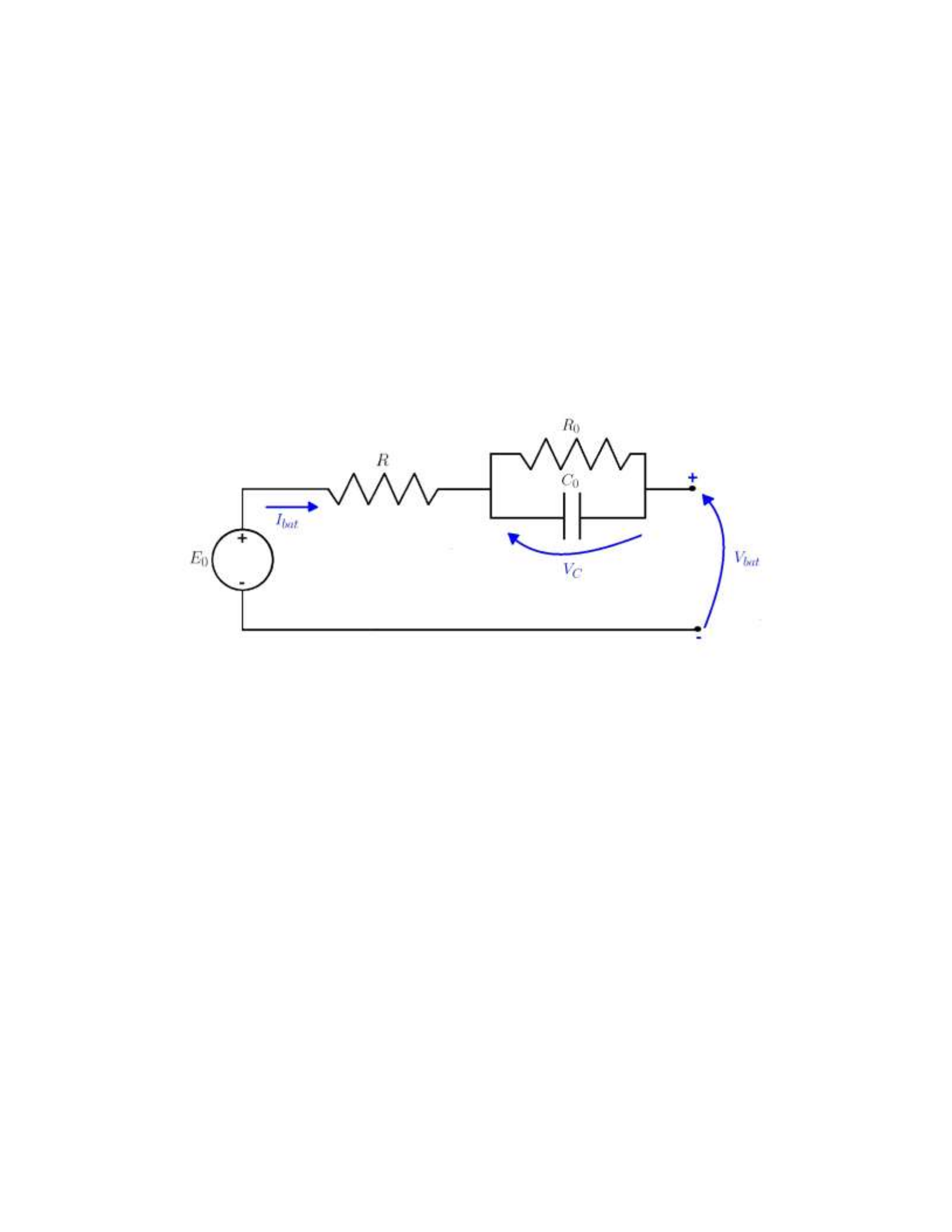
In this work, the dynamics of the battery are modeled as a 1st order Randle equivalent
circuit [25]. Figure 17 depicts the equivalent circuit used in the model, with the relevant
model parameters.
Figure 17: First-Order Battery Equivalent Circuit Model
The model consists of an ideal voltage source, 𝐸0, a linear resistive element, R, and a
parallel combination of a resistor and capacitor, 𝑅0 and 𝐶0, connected in series with the
voltage source and resistive element. The battery voltage, as observed at the battery
terminals, may be determined from the following circuit equation:
𝑉𝑏𝑎𝑡 = 𝐸0 − 𝑅𝐼𝑏𝑎𝑡 − 𝑉𝑐 (5)

29
The dynamics of the battery voltage are therefore contingent upon the capacitive term
(𝑉𝑐) in Equation 5. The governing equation for the voltage drop across 𝑅0 and 𝐶0 can be
expressed as follows [26]:
𝑑𝑉𝑐 𝑉𝑐 𝐼𝑏𝑎𝑡 (6)
In order to fully define the battery model, it is necessary to calibrate the four battery
parameters: 𝐸0, 𝑅, 𝑅0 and 𝐶0. It is common practice to model these parameters as
functions of the battery state of charge (SOC), temperature (𝑇𝑏𝑎𝑡), C-rate, and the sign of
the battery current [27, 28]. To reduce the complexity of the required calibration
procedure and the resulting parameter maps, the sign of the battery current and the C-rate
are combined into a single variable, termed the current level (𝐼𝑙𝑒𝑣𝑒𝑙). The battery SOC and
current level are defined as follows:
(7)
(8)
Where 𝐴ℎ𝑛𝑜𝑚 is the nominal battery capacity in ampere-hours, 𝑆𝑂𝐶0 is the initial battery
capacity, and 𝑠𝑖𝑔𝑛(𝐼𝑏𝑎𝑡) denotes the sign of the battery current (positive for discharge,
negative for charge).
The battery parameters can therefore be expressed in the following form:
𝐸0 = 𝑓(𝑆𝑂𝐶, 𝑇𝑏𝑎𝑡) (9)

30
𝑅, 𝑅0, 𝐶0 = 𝑓(𝑆𝑂𝐶, 𝑇𝑏𝑎𝑡, 𝐼𝑙𝑒𝑣𝑒𝑙) (10)
The calibration and validation of the battery model required a thorough set of experiments,
which were performed on the battery test bench described in Section 2.1.3. Specific
testing procedures were engineered to provide a set of experimental data that allowed for
separately calibrating the key model parameters.
Prior to the identification of the equivalent circuit parameters, the nominal capacity
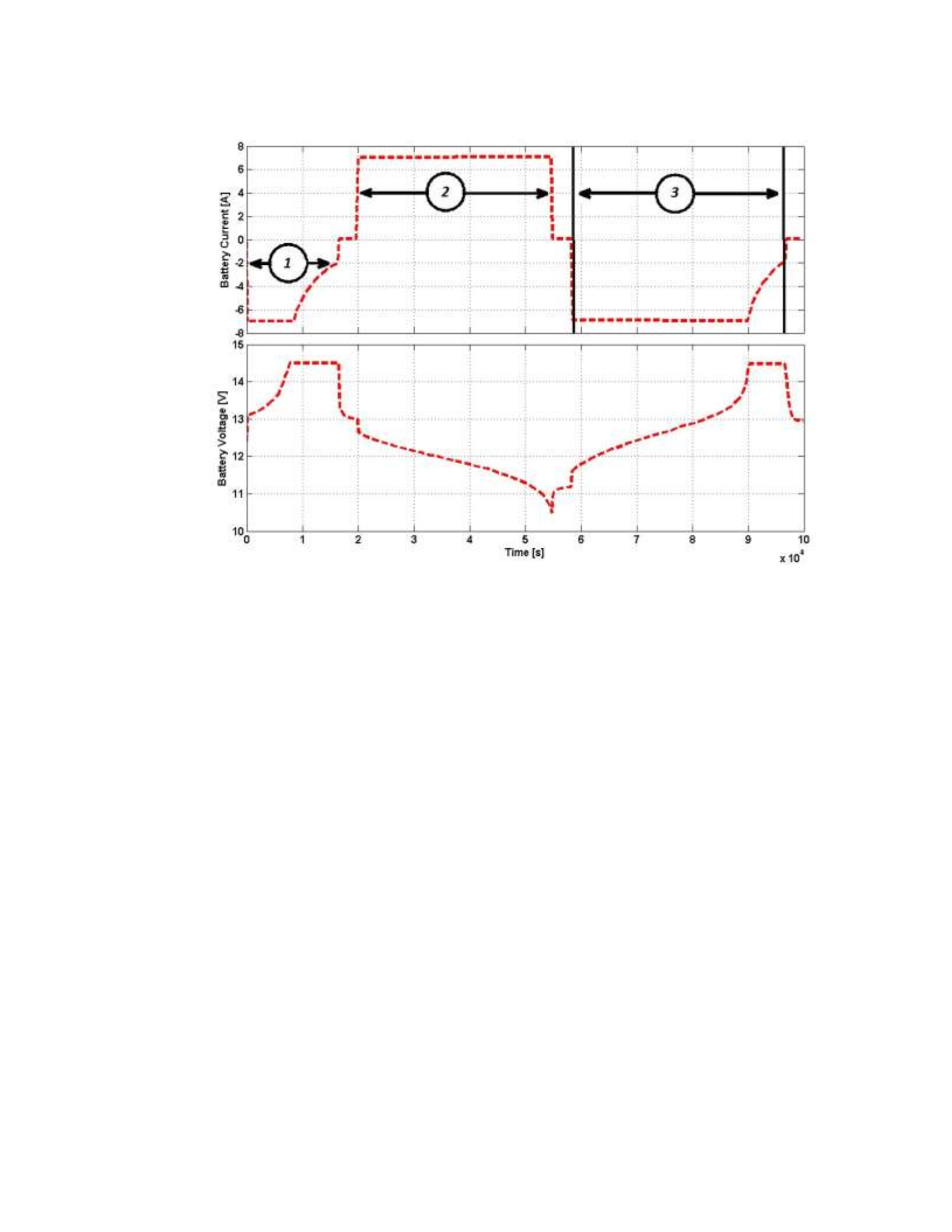
(𝐴ℎ𝑛𝑜𝑚) of the battery was determined. This procedure is outlined as follows, and is
graphically depicted in Figure 18 for clarity:
1. The battery is fully charged utilizing a CC-CV (constant current, constant voltage)
profile.
2. The battery is fully discharged at a constant current of 0.1C.
3. The battery is then fully charged to the upper voltage threshold by using a CC-CV
profile.
31
Figure 18: Current and Voltage Profile for Battery Capacity Test
The battery is considered fully discharged when the battery voltage reaches 10.5 V.
Similarly, the battery is considered fully charged when the battery voltage reaches 14.5 V
and the battery current drops below 2 A. The charge and discharge capacities (determined
by steps 2 and 3, respectively) are then averaged, resulting in a nominal battery capacity
of 72.3 Ah. This procedure was only performed once in order to minimize the excessive
battery aging that would be induced by the deep-cycling of a flooded lead-acid battery.
The aging may manifest itself as sulfation on the plates of the lead-acid battery, reducing
the apparent battery capacity and increasing the internal resistance [29].

32
The second experimental test conducted on the battery was oriented towards the
determination of the open-circuit voltage (𝐸0) which is generally assumed a function of
the battery SOC and temperature [27, 28]. The experimental procedure designed for
determining 𝐸0 is summarized as follows:
1) The battery is fully discharged.
2) The battery is charged at a constant current level in order to increase the battery
SOC by 5%.
3) The battery is rested sufficiently, and the open-circuit voltage is approximated as
the voltage measured across the battery terminals.
4) Steps 2 and 3 are repeated until the battery is charged to 100% SOC
5) The battery is discharged at a constant current level in order to decrease the battery
SOC by 5%.
6) The battery is rested sufficiently, and the open-circuit voltage is approximated as
the voltage measured across the battery terminals.
7) Steps 5 and 6 are repeated until the battery is completely discharged.
8) The battery is charged to 100% SOC.
9) Steps 1-8 are performed at temperatures of 25C , 40C , and 50C . From the above
procedure, two curves were generated for each temperature, one describing the
relationship between the open-circuit voltage and the battery SOC when the
battery is charging, and a similar curve for battery discharge. The two curves were
then averaged to produce the open-circuit voltage 𝐸0 as a function of the battery
state of charge. The results for all three battery temperatures is illustrated in
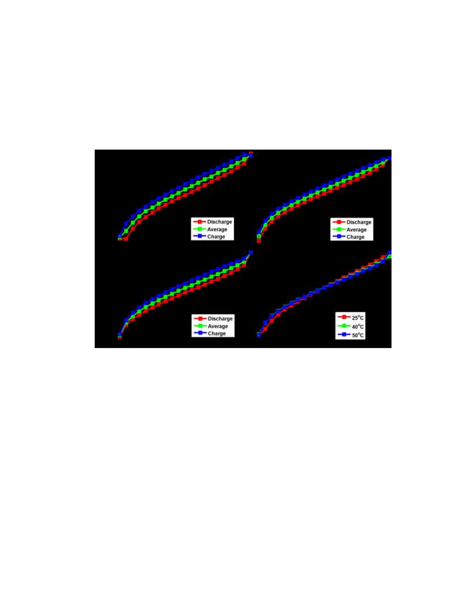
33
Figure 15. The upper-left, upper-right, and lower-left plots show the open-circuit
voltage curves for temperatures of 25, 40, and 50 degrees Celsius, respectively.
The lower right plot shows the averaged open-circuit voltage plots for all three
temperatures.
Battery SOC [%] Battery SOC [%]
Figure 19: Summary of the Open-Circuit Voltage Characterization Test.
Finally, the equivalent circuit model parameters, 𝑅, 𝑅0, and 𝐶0 were all determined
through a single, extensive test where a transient current profile was imposed by the
programmable load and supply system. In order to develop a model accurate for a wide
range of operating conditions, the battery was subjected to numerous current levels and
current steps of varying magnitude. The parameter values were then averaged across all

34
current steps at each current level. A brief summary of this experimental procedure is
detailed as follows:
1) The battery is charged to 100% SOC utilizing a CC-CV profile
2) A current profile composed of numerous current levels and current steps of various
magnitudes and sign is imposed on the battery.
3) The battery is discharged at constant current to a new state of charge.
4) Steps 2 and 3 are repeated until a predetermined cutoff SOC is reached.
5) Steps 1-4 are performed at temperatures of 25C , 40C , and 50C .
Figure 20 illustrates the parameter identification procedure, evaluated for just one battery
SOC value. The numbers in the figure indicate the current profile for steps 1, 2 and 3
described above.

35
Figure 20: Current Profile for the Identification of Battery Model Parameters.
The values for 𝑅, 𝑅0, and 𝐶0 were then determined following the identification procedure
described in [30].
Following the initial calibration procedure, the model parameter values were smoothed
with respect to the battery state of charge and current level in order to ensure continuity of
the predicted voltage output. This task was performed by first developing a “surface” of
battery parameter values for each battery temperature considered. Each surface was then

36
fit with a 5th order polynomial with respect to both the battery SOC and current level. The
resulting parameter maps were found to be consistent with the experimental data,
providing a smooth transition between battery operating points, and being consistent with
the expected behavior typically exhibited by equivalent circuit battery model parameters
(such as a growth in internal resistance due to a higher charging current) . Furthermore,
the battery is not expected to operate outside of the SOC range considered during
calibration, making smoothing of the battery parameters via curve-fitting a reasonable
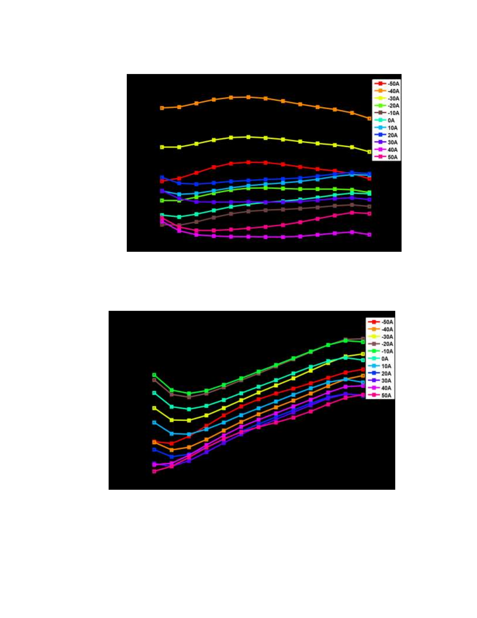
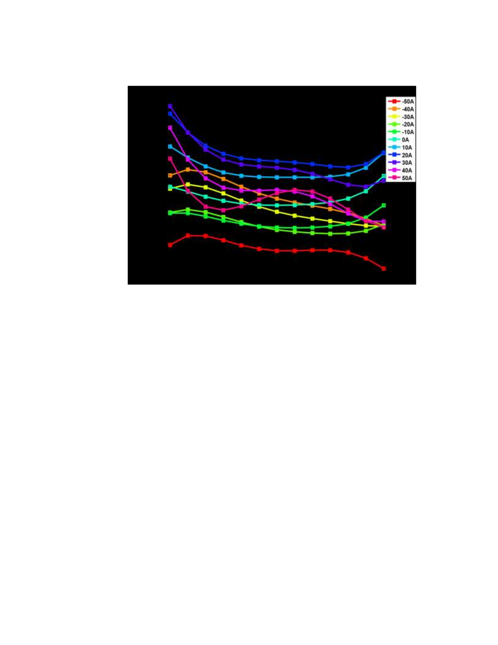
approach. Figures 21, 22, and 23 illustrate the smoothed calibration results for 𝑅, 𝑅0, and
𝐶0 (respectively) at a temperature of 40C .
37
x 10-3 I
10 level
Battery SOC [%]
Figure 21: Battery Model Parameter Identification: Parameter R for 40 C
0.035
I
Battery SOC [%]
38
Figure 22: Battery Model Parameter Identification: Parameter 𝑹𝟎 for 40 C
Battery SOC [%]
Figure 23: Battery Model Parameter Identification: Parameter 𝑪𝟎 for 40 C
From Figures 21 and 22, the battery internal resistances (𝑅, 𝑅0) are observed to increase
overall as the battery current changes directions from discharging to charging. This is to
be expected, as the charge acceptance of the battery is expected to decrease as charging
currents of larger and larger magnitudes are imposed. As the battery state of charge is
increased towards 100%, the internal resistance (R) is also expected to increase
significantly. However, this behavior is not depicted in Figure 21 due to the SOC only
achieving a value of approximately 98%. Of particular interest in this experiment is the
dependence of the battery parameters on the temperature (𝑇𝑏𝑎𝑡), as the temperature of the
air and mounting brackets surrounding an automotive battery are expected to fluctuate
39
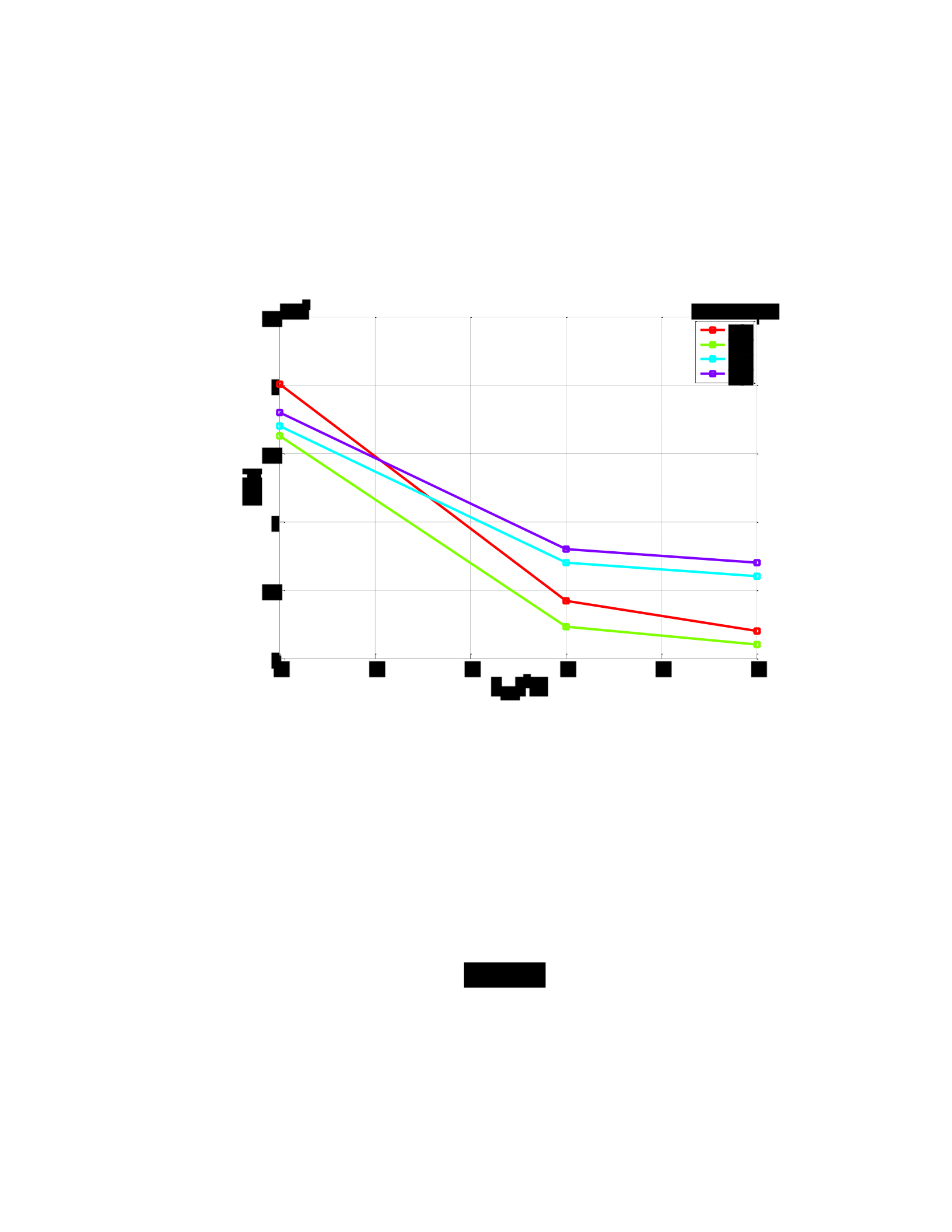
heavily depending on the particular testing environment. Figure 24 illustrates the
temperature-dependence of the battery internal resistance for 𝐼𝑙𝑒𝑣𝑒𝑙 = 50𝐴. Note that not
all constant-SOC lines are plotted to avoid overcrowding of the figure.
Figure 24: R-values as a function of Battery Temperature
The internal resistance of the battery exhibits an approximately inverse relation with the
battery temperature. While Figure 24 only depicts this relationship for a single current
level, a large portion of the internal resistance map is consistent with these findings. This
behavior can be attributed to the well-known Arrhenius Equation:
(11)
25
30
35
40
45
50
3
3.5
4
4.5
5
5.5
x 10
-3
T
bat
[
o
C]
Battery SOC
%
83
%
86
%
95
%
97

40
Where k is the rate constant of the chemical reaction, 𝐸𝑎 is the activation energy, R is the
universal gas constant, and T is the absolute temperature in degrees Kelvin. According to
Equation 11, as the temperature increases, the rates of the chemical reactions occurring
within the battery increase significantly. This facilitates faster current transport,
translating to a lower internal resistance. With the internal resistance maps largely in
agreement with this, confidence in the calibration of the battery parameters may be
achieved.
2.3.3: Chrysler EVR Controller Model
As the motivation for this project is to demonstrate the ability of a supervisory controller
to provide improved fuel economy through the intelligent management of the vehicle
electrical system, some baseline for comparison is necessary. The control strategy
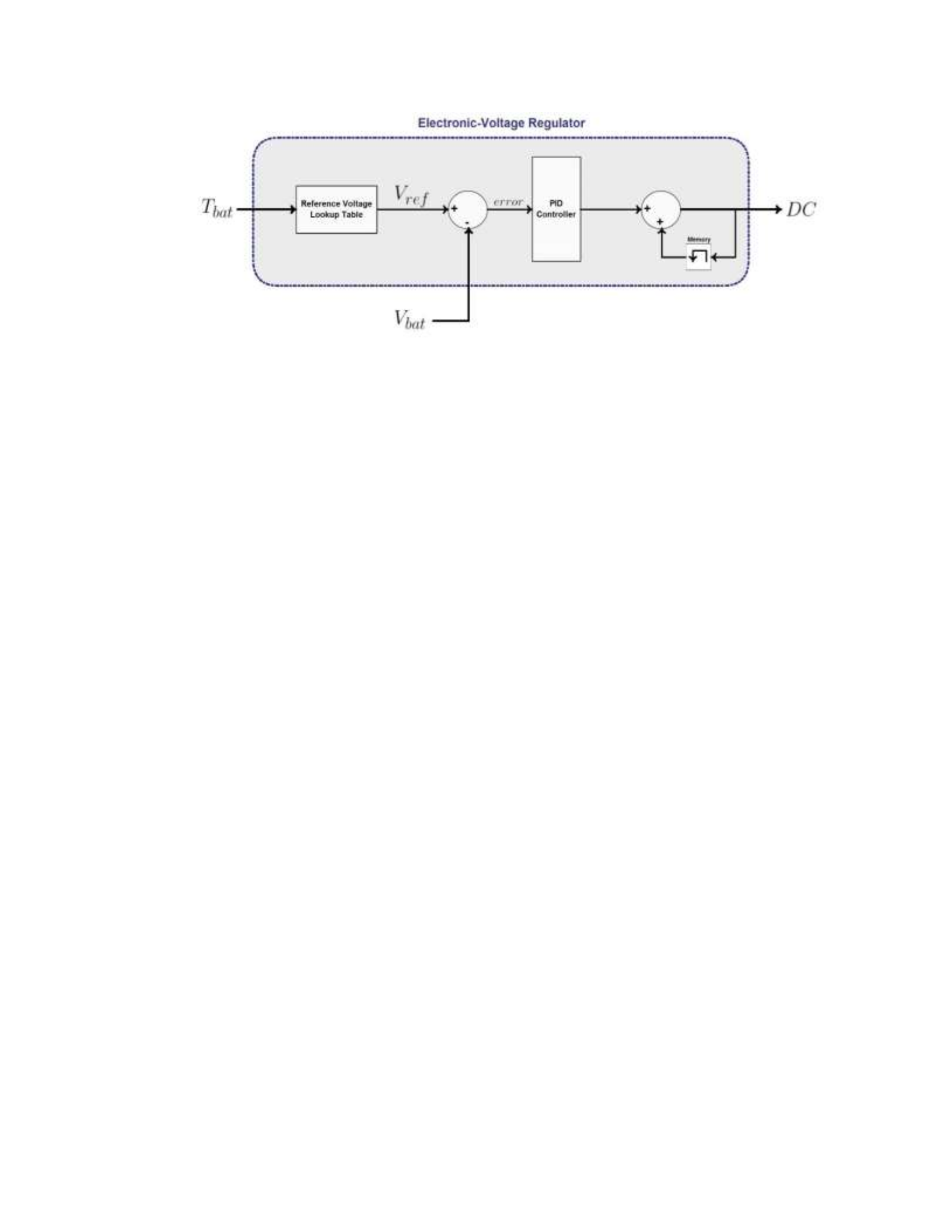
currently employed in the vehicle is termed the Electronic-Voltage Regulator (EVR). The
EVR compares some temperature-dependent reference battery voltage with the
immediate battery voltage, and attempts to minimize the difference between the two by
commanding the alternator duty cycle. Given this information, a model of the EVR is
then developed and tuned to agree with experimental data. A block diagram depicting the
general underlying logic of the EVR controller may be studied in Figure 25.
41
Figure 25: Electronic-Voltage Regulator Block Diagram
Calibration of the EVR was achieved through trial-and-error in regards to both the
reference-voltage lookup table and the PID-controller parameters.
2.3.4: Vehicle Electrical System Model Validation
In order to ensure the validity of the alternator and battery models in a standalone
environment and guarantee compatibility between all sub-components of the vehicle
electrical system, each VES sub-model is first validated independently with experimental
data collected via the ETAS ES1000. The entire model is then validated with the same on-
road experimental data. This experimental data is collected over a wide range of operating
conditions by subjecting the vehicle to an on-road driving cycle with the airconditioning
(A/C) system switched to automatic to create a variable load current profile. The vehicle
velocity, engine torque and speed, and vehicle electrical load are all depicted for this drive
cycle in Figure 26. Take note that a significant portion of this experimental data was
collected on the highway.

42
Figure 26: VES Validation Experimental Data.
The standalone alternator model results are compared with the experimental data in Figure
27. The RMS error over the entire timespan of the on-road cycle is 5.1 A, or
4.5%.
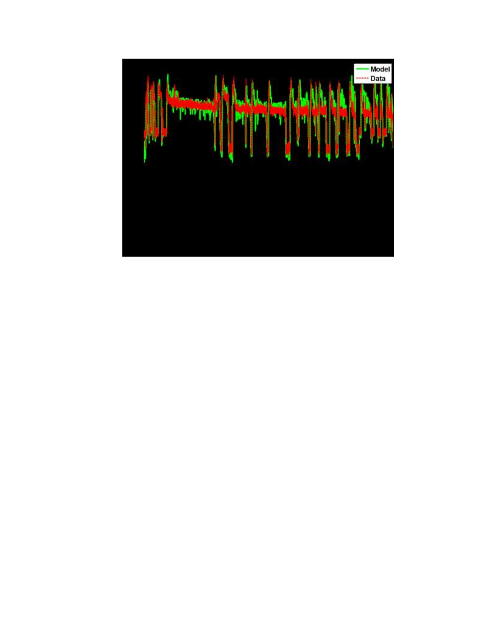
43
Figure 27: Results of Standalone Alternator Model Validation.
In order to ensure the legitimacy of the battery parameter maps outside of the range of
calibration, a verification of the standalone battery model is performed. In conjunction
with the verification of the alternator model, experimental data extracted from the onroad
drive cycle with the A/C set to automatic mode is used to mimic realistic driving
conditions. Figure 28 illustrates the electrical current input to the battery model, as well
as both the experimental and simulated battery voltages. The RMS error over the entire
drive cycle is 0.25 V, or 1.8%. Given the wide range of operating conditions that the
vehicle is subjected to for this on-road driving cycle (i.e. city and highway driving, A/C
and radiator fan switching on/off, etc…) this error may be considered acceptable.

44
Figure 28: Results of Standalone Battery Model Validation.
Figures 29 and 30 depict the experimental battery voltage and alternator current
(respectively) alongside the simulation results for the assembled vehicle electrical system
model. Note that the inaccuracies of each sub-model amplify as the entire vehicle
electrical system model is assembled. The RMS error of the battery voltage is 0.26 Volts,
whereas the RMS error of the alternator current is 8.4 A.
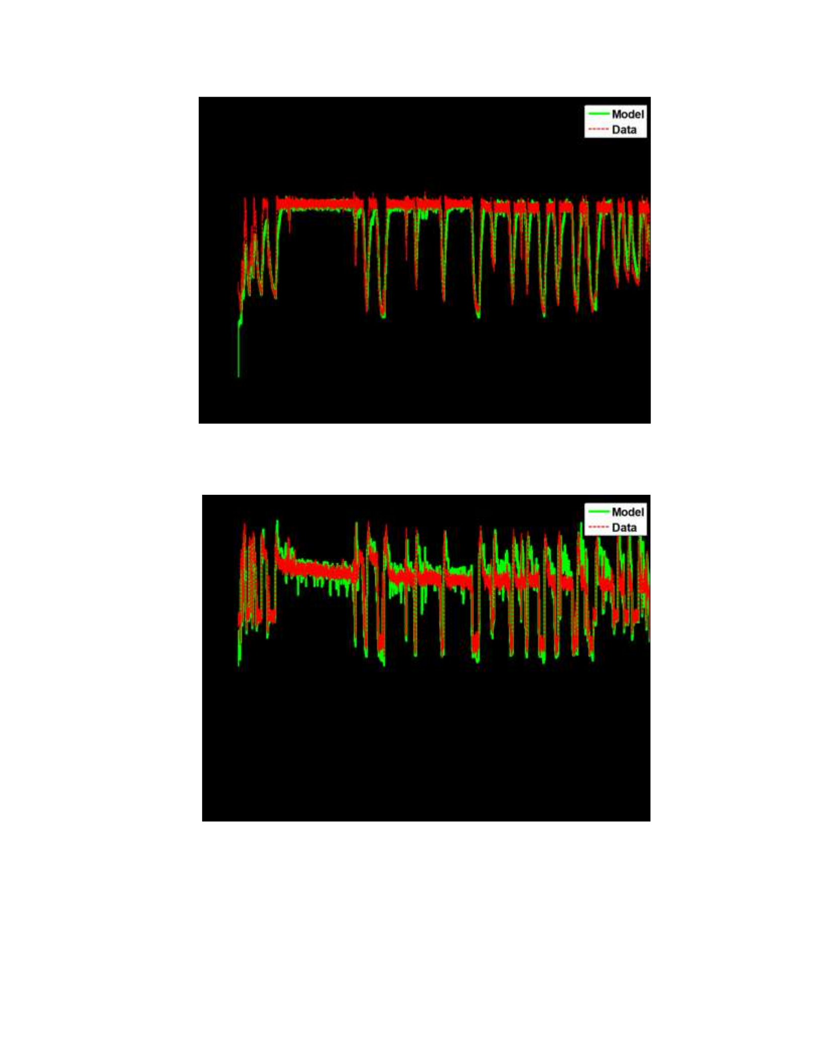
45
Figure 29: Full Vehicle Electrical System Validation: Battery Voltage.
Figure 30: Full Vehicle Electrical System Validation: Alternator Current.

46
The increase in the overall predictive error of the electrical system model, and in
particular the alternator sub-model, is more than likely due to the inaccuracies of each
subsystem compounding upon one another. The model calibration procedures utilized for
developing the alternator model, which obtains quasi-static steady-state data points, may
be partially to blame for these inaccuracies. A design of experiment which is able to take
into account the dynamics of the alternator may yield a more accurate VES model.
Referencing [31], a mean-value approach may be taken towards alternator modeling
which includes lumped inductances and a bridge rectifier circuit and takes into account
the fast dynamics of the alternator, and results in a very good match with experimental
data over a wide range of operating conditions. However, given that the fast dynamics of
the vehicle electrical system are not of crucial importance when evaluating cumulative
vehicle fuel consumption over an extended period of time such as a drive cycle, this error
is acceptable for the purposes of developing the energy supervisory controller. As an
investigation into the effects of the VES model inaccuracies, the cumulative energy error
of the battery over the drive cycle under consideration is studied. This is achieved
through simply taking the integral of the product of the battery voltage and current over
the entire drive cycle for both the experimental and model data sets. The results of the
accumulated energy within the battery, for both the model and experimental data, are very
similar and are summarized in Table 3.
Table 3: Impact of VES Model Inaccuracies on Accumulated Battery Energy
Data Source
𝑬𝒃𝒂𝒕 Accumulated (kWh)

47
Model
-0.07
Experimental
-0.06

48
Chapter 3: Application of Optimal Control Theory to the Energy
Management of a Vehicle Electrical System
An accurate baseline controller, the Electronic Voltage Regulator, for evaluating the
performance of an energy management control strategy has been developed in Chapter 2.
While fuel economy improvements upon this baseline controller may be quantified, it is
necessary to establish an understanding of the maximum possible fuel savings that may be
recognized. Optimal control theory allows for a relatively straightforward solution to this
objective by addressing the issue of finding the control input trajectory which optimizes a
specific performance criterion [32], i.e. minimization of the cumulative vehicle fuel
consumption. Therefore, the application of optimal control theory to the energy
management of a vehicle electrical system provides a useful benchmarking tool to
evaluate the efficacy and performance of implementable, sub-optimal control strategies.
The present chapter investigates the potential benefits of optimal control theory, as applied
to the vehicle electrical system.
Chapter 3 begins with a discussion of the optimal control problem and objectives. An in-
depth analysis of optimal control over a single drive cycle, as applied to the VES, is then
performed. The robustness of the control strategy is then investigated through various
sensitivity analyses. Finally, this analysis is expanded to numerous scenarios, and the
overall behavior of the optimal control strategy is characterized.

49
Section 3.1: Optimal Control Objectives and Methodology
The control problem, specific to the vehicle electrical system under investigation, is first
defined in this section. Electrical system constraints are then discussed, followed by an
application-specific derivation of the selected optimal control solution.
3.1.1: Alternator-Battery Power Split Problem
The primary objective put forth is to improve the overall fuel economy of a vehicle
through the development of a new electrical system control strategy. The currently
employed control strategy, termed “Electronic-Voltage Regulation” (or EVR for short)
maintains battery voltage at a predetermined value in order to ensure a full charge, only
utilizing the battery when the alternator is incapable of providing the desired load. While
this control strategy provides for reliable cold-cranking conditions, it is inherently
inefficient for two reasons:
1) The charge acceptance of lead-acid batteries drops off considerably when fully
charged, resulting in unnecessary system losses.
2) Holding the battery to a near-constant state of charge negates many of its potential
benefits as a dynamic, on-board energy storage system.
The development of a less conservative control strategy (with respect to the battery’s cold
cranking ability), which can exploit the battery’s ability to function as a reversible energy
storage device, may therefore prove beneficial to vehicle fuel economy. Such control
strategies are commonplace in hybrid electric vehicles, being utilized to optimize the
“power-split” between the engine and electric motor. The overall architecture of a

50
conventional automotive electrical system is quite similar to that of a mild, parallel HEV.
It is therefore reasonable to develop an electrical system control strategy for use in a
conventional automobile centered around a similar “current-split” principle. A block
diagram depicting the vehicle electrical system of interest, and its interactions with the
engine, may be observed in Figure 31.
Figure 31: Vehicle Electrical System Schematic
Take note that 𝑇𝑒𝑛𝑔 refers to the baseline engine torque, which is equivalent to the engine
brake torque minus the torque required to drive the vehicle alternator. During data
acquisition, however, it is impossible to decouple these two torques from one another, as
the vehicle ECU calculates the approximate net engine torque. Therefore, in order to
approximate the baseline engine torque as closely as possible, the vehicle electrical loads
(and therefore the alternator torque) are minimized during all experimental data collection
discussed in Chapter 3. The effects of the alternator torque on the calculated net engine

51
torque therefore result in a small, near-constant offset error which may be neglected for
the purposes of the analyses performed.
Referencing Figure 31, it can be seen how the current-split is directly tied in to the vehicle
fuel consumption. Determining the optimal current-split between the battery and
alternator, via the alternator duty-cycle command, is therefore the control problem of
interest. The optimal current-split is therefore defined as the control command which
fulfills the following criteria:
1) Provides the desired current to the electrical loads at any given point in time;
2) Splits the current demand between the battery and alternator so to minimize energy
consumption in relation with the operating conditions of the system;
3) Satisfies a set of constraints on battery and electrical system performance.
The latter of these requirements will be evaluated in the following section.
3.1.2: Constraints of the Vehicle Electrical System
Constraints on the vehicle electrical system, administered by the control strategy, are put
in place in order to ensure driver comfort and safety and avoid damaging the alternator
and coupled electrical loads, while the detrimental battery-aging effects that accompany
rapid current and voltage swings are regulated and kept to a minimum. The exact form of
these constraints is explicitly laid out as follows:
𝑉𝑚𝑖𝑛 ≤ 𝑉𝑏𝑎𝑡(𝑡) ≤ 𝑉𝑚𝑎𝑥 (12)
𝐼𝑏𝑎𝑡,𝑚𝑖𝑛 ≤ 𝐼𝑏𝑎𝑡(𝑡) ≤ 𝐼𝑏𝑎𝑡,𝑚𝑎𝑥 (13)

52
𝐼𝑎𝑙𝑡(𝑡) ≤ 𝐼𝑎𝑙𝑡,𝑚𝑎𝑥 (14)
(15)
Where constraint 1 represents the minimum and maximum allowable battery
voltages, and ensures that all electrical loads in the vehicle remain operating within
specification (ex. cabin lights and blowers maintaining acceptable operating
voltages). Constraint 2 represents the minimum and maximum allowable battery
currents, and is enacted for similar reasons. Constraint 3 represents the maximum
possible alternator current (which is dependent upon operating conditions), and
constraint 4 represents the maximum allowable battery voltage time rate of change.
The implementation of these constraints is carried out by means of defining a
currentsplit array (γ) which, in conjunction with the maximum alternator current
value, provides a discrete representation of all possible current-split options within
the vehicle electrical system. The derivation of the current-split procedure is laid out
below. From this point forward, all variables in bold font exist as vectors.
𝜸 = [0, 1] ∈ ℝ𝑛 (16)
𝑰𝒂𝒍𝒕 = 𝜸 ∙ 𝐼𝑎𝑙𝑡,𝑚𝑎𝑥
(17)
𝑰𝒃𝒂𝒕 = 𝐼𝑙𝑜𝑎𝑑𝑠(𝑡) − 𝑰𝒂𝒍𝒕
(18)
Where 𝐼𝑙𝑜𝑎𝑑𝑠(𝑡) represents the electrical load demand in amperes. The resultant battery
current array is passed through a 0th-order simplified battery model having the ability to
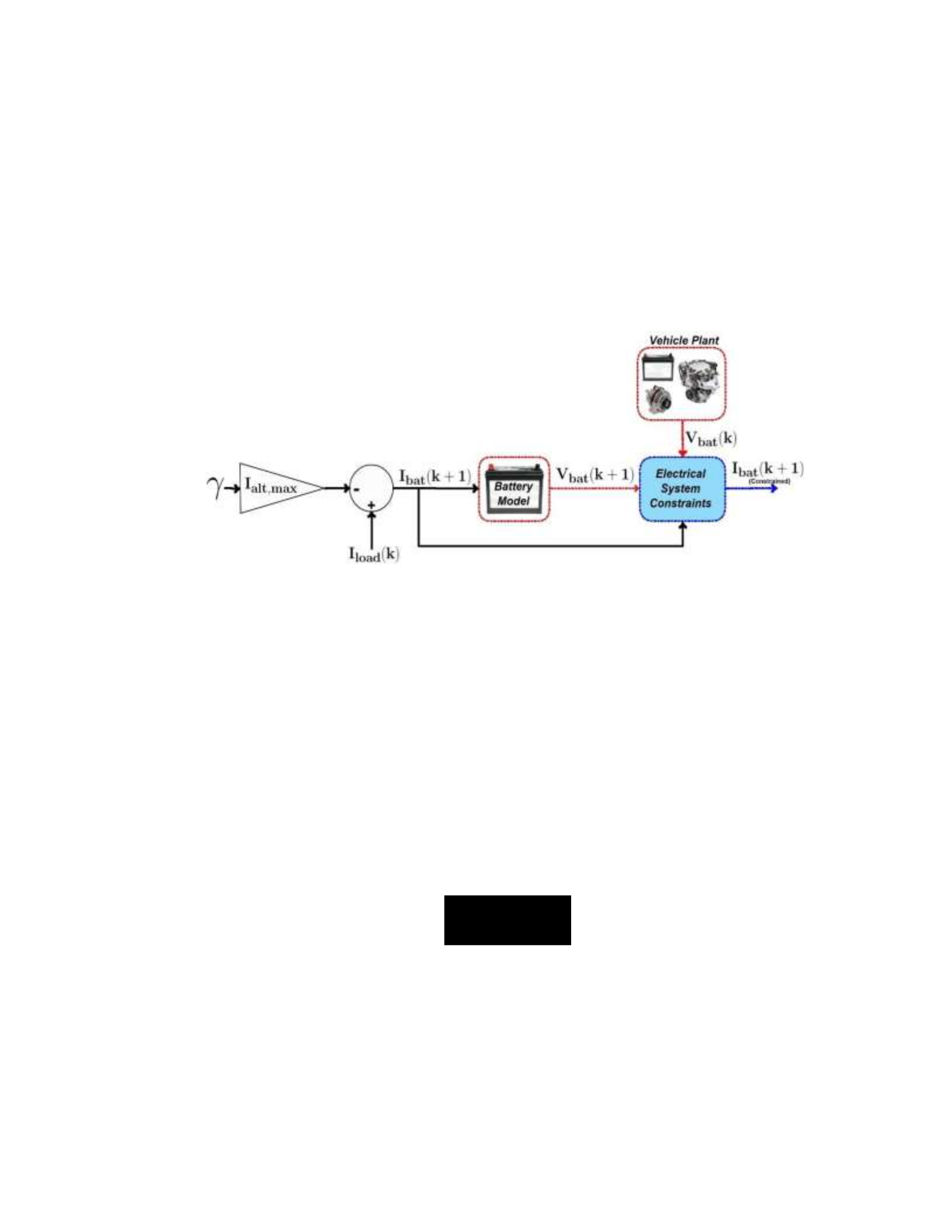
53
approximate future battery voltage, given the battery’s present state and future current
level. Any battery current values that result in violations of the constraints can then be
filtered out before the remaining suitable candidates are passed on to the next step in the
control process. Figure 32 graphically depicts the general structure of how the system
constraints are implemented in the energy management strategy.
Figure 32: Implementation of Vehicle Electrical System Constraints
3.1.3: Optimal Control with Pontryagin’s Minimum Principle
The desired outcome of the energy management strategy under consideration is the
minimization of cumulative vehicle fuel consumption over a given drive cycle while
sustaining battery charge. To this extent, a global optimal control problem may be
formulated. An integral cost function, J, is first defined as follows:
(19)
Mathematically speaking, the optimal control solution 𝑢∗(𝑡) may be described as the
control trajectory which minimizes this integral cost function. As may be observed in

54
Figure 32, the fuel mass flow rate depends in part on the alternator torque, which may
ultimately be expressed as a function of the battery state of charge x(t) and battery power
u(t). Therefore, the following may be stated:
(20)
The evolution of the vehicle electrical system in time may be described by a differential
equation which relates the battery SOC to the battery power:
(21)
A negative current value signifies charging. In order to utilize optimal control theory, it is
necessary to restructure Equation 21 such that the time rate of change of the battery state
of charge is explicitly dependent upon the battery state (SOC) and control input (𝑃𝑏𝑎𝑡).
This may be performed by analyzing the simplified battery model, featured in
Figure 33 and referenced in Section 3.1.2.
Figure 33: 0th-order Battery Model

55
(22)
(23)
(24)
By substituting Equation 23 into Equation 22, and recalling that both the open-circuit
voltage and internal resistance are functions of the battery state of charge, the battery
voltage can be expressed as an explicit function of the state and control variables. The
resulting equation may then be plugged into Equation 24, which allows for the electrical
system dynamics to be rewritten as follows:
Where 𝜑(𝑥, 𝑢, 𝑡) = 𝐼𝑏𝑎𝑡(𝑡).
Subject to the system constraints discussed in Section 3.1.2, as well as:
𝑥(𝑡0) = 𝑥0 (26)
𝑥(𝑡𝑓) = 𝑥𝑓 = 𝑥0 (27)
𝑥𝑚𝑖𝑛 ≤ 𝑥(𝑡) ≤ 𝑥𝑚𝑎𝑥 (28)
Due to the constrained nature of the optimization problem at hand, Pontryagin’s Minimum
Principle proves particularly useful and may be utilized in order to account for both the
upper and lower bounds on the battery state of charge, as well as the required charge-
sustaining behavior of the battery. The global optimal control problem can then be recast

56
into a local optimization problem. This is achieved by introducing a timevarying
Lagrange multiplier, or co-state variable, λ, alongside a boundary penalty function, or
inequality constraint, μ, which arises from the Karush-Kuhn-Tucker conditions. An
extended Hamiltonian function, H, may then be developed such that the following
necessary conditions are satisfied:
𝐻(𝑥∗, 𝑢∗, 𝜆∗, 𝜇∗, 𝑡) ≤ 𝐻(𝑥, 𝑢, 𝜆, 𝜇, 𝑡) ; ∀𝑢 ≠ 𝑢∗ (29)
𝑥∗(𝑡𝑓) = 𝑥∗(𝑡0) = 𝑥0 (30)
𝑥 ∗(𝑡) = ∇𝜆𝐻|∗ (31)
𝜆 ∗(𝑡) = ∇𝑥𝐻|∗ (32)
Where the Hamiltonian function is defined as follows:
(33)
The objective being to minimize the Hamiltonian function at each time step. In order to
apply this optimization method to the vehicle electrical system, analytical expressions for
both the co-state variable λ and the boundary function μ are developed as follows:
(34)
𝜇𝑙 𝑆𝑂𝐶 ≥ 𝑆𝑂𝐶𝑚𝑎𝑥
𝜇(𝑡) = {−𝜇𝑙 𝑆𝑂𝐶 ≤ 𝑆𝑂𝐶𝑚𝑖𝑛 ; (𝜇𝑙 ≥ 0)
0 𝑒𝑙𝑠𝑒
(35)
The computationally intensive parameters, , may be solved off-line and mapped
vs. the battery SOC (state), power (input), and temperature to allow for rapid calculation
of the co-state dynamics in real-time. These maps are shown in Figure 34 for a
temperature of 40 deg. C.

57
Figure 34: Co-state Dynamics Lookup Tables at 40 deg. C
The minimum (optimal) value of the Hamiltonian may now be located. For each discrete
time step that the Pontryagin control strategy is triggered, the duty cycle command which
results in this minimum Hamiltonian is fed back to the alternator, completing the
closedloop control circuit. The optimal control problem, now fully defined, may be
summarized according to Figure 35. Take note of the contrast between the inputs of the
inverted alternator maps in Figure 35, and the alternator maps featured in Figure 16. The
inverted maps monitor the battery voltage, engine speed, and the alternator current array,
and output a corresponding duty-cycle and alternator torque array. This duty-cycle array
is passed through an index function which monitors the position of the minimum
Hamiltonian function, and outputs the corresponding duty-cycle command.
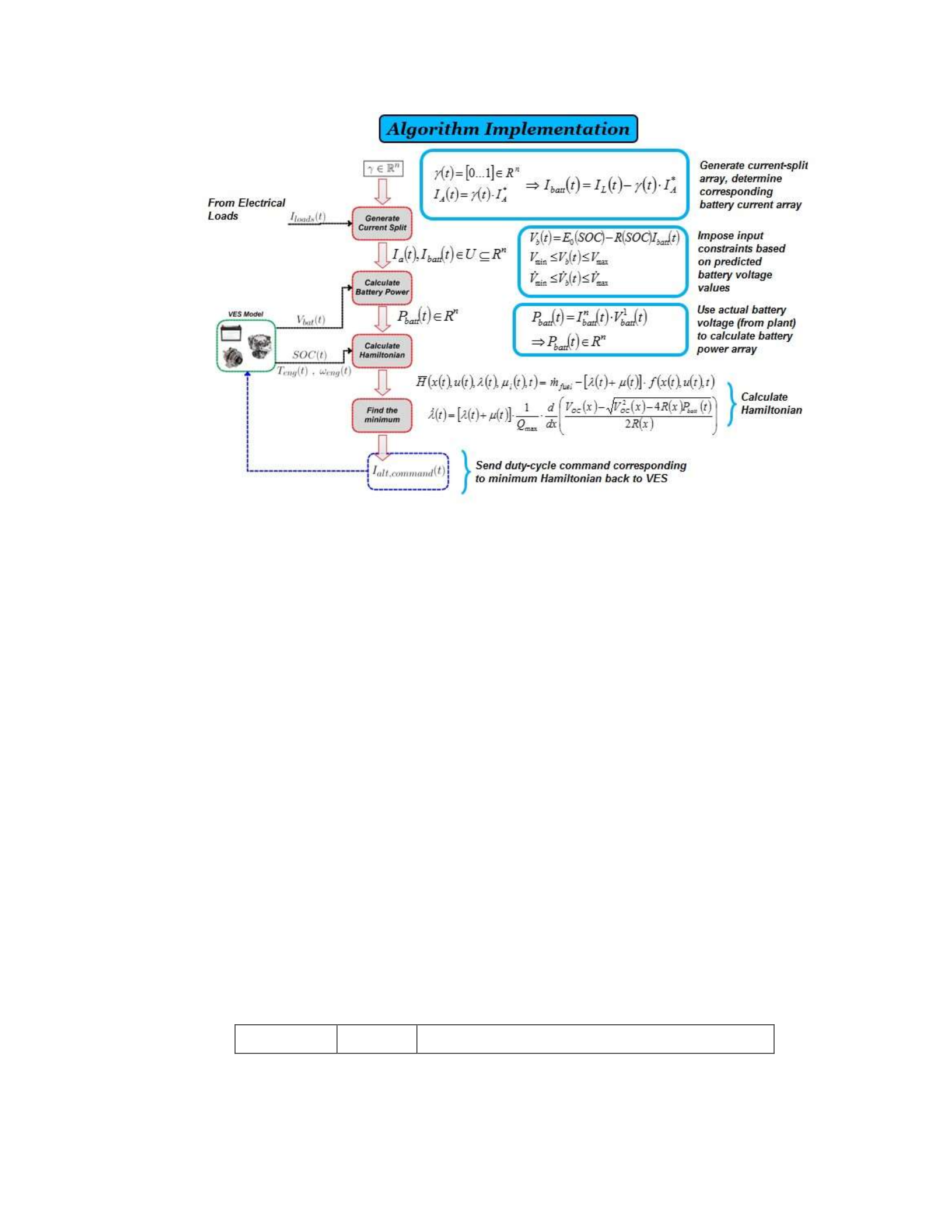
58
Figure 35: Structure of Pontryagin’s Minimum Principle Control Strategy
The values of the electrical system constraints implemented into the control strategy, as
well as the limitations on the operating conditions of the battery SOC, are defined in
Table 4.
Table 4: Vehicle Electrical System Constraints
Parameter
Value
Description

59
𝑽𝒎𝒊𝒏
11.5 V
Minimum battery voltage
𝑽𝒎𝒂𝒙
15 V
Maximum battery voltage
𝑽 𝒎𝒂𝒙
0.5 V/s
Maximum rate of change of battery voltage
𝑰𝒃𝒂𝒕,𝒎𝒊𝒏
-50 A
Minimum battery current
𝑰𝒃𝒂𝒕,𝒎𝒂𝒙
50 A
Maximum battery current
𝑰𝒂𝒍𝒕,𝒎𝒂𝒙
150 A
Maximum alternator current
𝑺𝑶𝑪𝒎𝒊𝒏
82 %
Minimum desired battery state of charge
𝑺𝑶𝑪𝒎𝒂𝒙
88 %
Maximum desired battery state of charge
𝑺𝑶𝑪𝟎
85 %
Initial value of battery state of charge
Section 3.2: Analysis of Pontryagin’s Optimal Solution
In order to gather a comprehensive understanding of the general behavior of the vehicle
electrical system and the resultant vehicle fuel consumption when subjected to optimal
control conditions, the VES will be evaluated in-depth for a specific drive cycle and
electrical load profile. The New European Driving Cycle (NEDC) is assessed in Section
3.2.2 due to its relatively smooth velocity profile, which aids in concisely illustrating the
various physical behaviors which are characteristic of Pontryagin’s Minimum Principle.
The electrical load profile is set to a constant value of 57.5 A, approximating the average
electrical load value of the Chrysler minivan over numerous NEDC dynamometer runs
with the A/C set to automatic. This analysis is then expanded upon in Section 3.2.3 by
performing numerous sensitivity studies in regards to the control parameters, allowing one
to partially assess the feasibility of an adaptive, optimal-based implementable control
strategy. A more broad analysis of the Pontryagin control strategy is performed in Section
3.2.4, encompassing various combinations of drive cycles and constant electrical loads.

60
3.2.1: Influence of Parameters
Prior to any vehicle controller and plant behavioral analysis, the optimal control solution
for a given velocity trace and electrical load must be located. The primary control
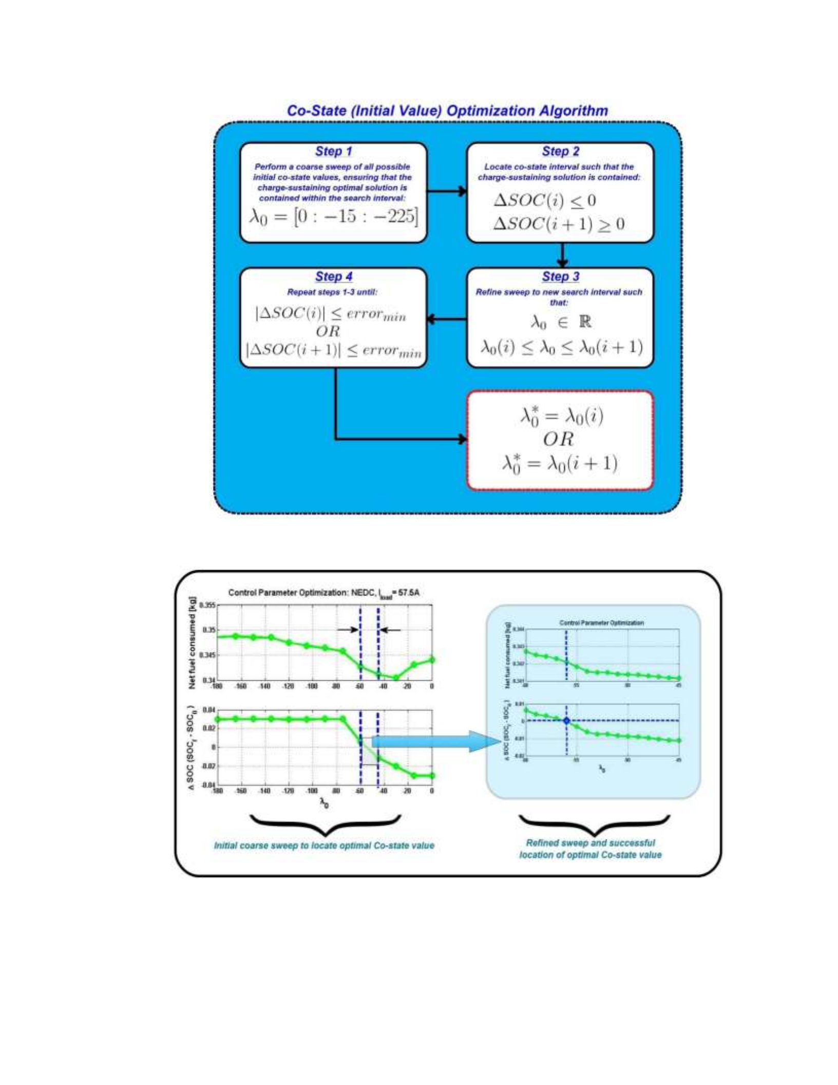
parameter which dictates charge-sustaining behavior is the initial value of the co-state
variable, 𝜆0. Therefore, by determining this value optimality may be ensured. An
optimization algorithm consisting of sequential “sweeps” across all potential co-state
candidates is implemented in order to locate the optimal value, . The algorithm first
searches for the appropriate co-state interval which contains a charge-sustaining solution.
Once this interval is determined, the search is refined and the procedure is repeated until
an acceptable degree of error (in regards to the net change of battery state of charge) is
achieved. A summary of the underlying structure of this algorithm is laid out in Figure 36.
For all drive cycles and electrical load values considered, the initial specified range of the
co-state variable (−225 ≤ 𝜆0 ≤ 0) is sufficient and contains the optimal solution. Figure
37 graphically depicts the location of for the case of the New European Drive Cycle
with the electrical load demand set to a constant 57.5A. The optimal initial costate value
for the particular scenario under consideration is determined in only two iterations and is
equal to -56. The optimal boundary penalty function is relatively easy to calibrate in
comparison; a significantly high value which prevents violation of the state constraints is
sufficient, thus μ may be held to a value of 400 for all driving scenarios.
61
Figure 36: Initial Co-state Variable Optimization Algorithm Outline
Figure 37: Initial Co-state Variable Optimization for NEDC, 𝑰𝒍𝒐𝒂𝒅𝒔 = 𝟓𝟕. 𝟓𝑨
62
3.2.2: Case Study Results: New European Drive Cycle
The vehicle fuel economy and electrical system behavior, subjected to optimal control, are
thoroughly investigated for a constant electrical load profile of 57.5A and the NEDC
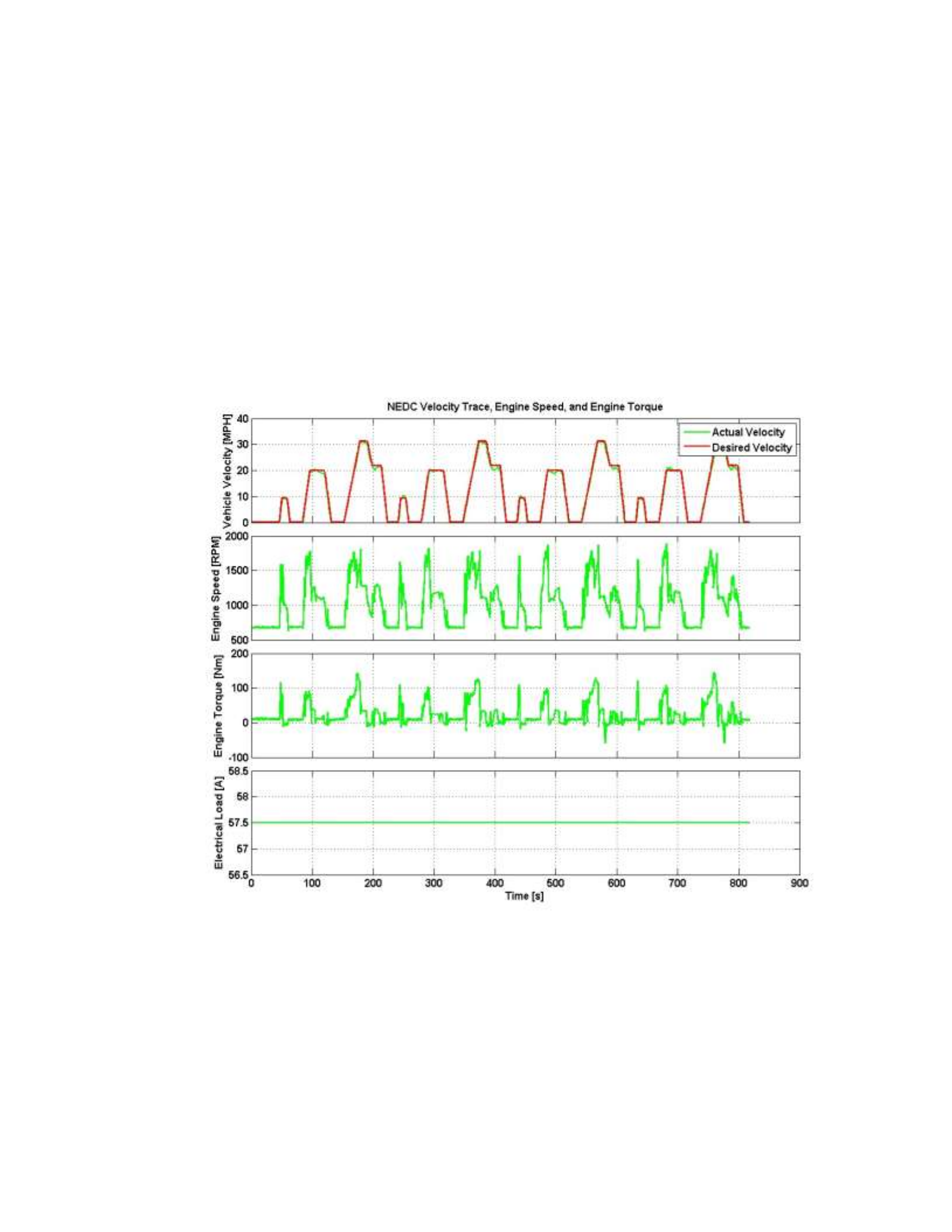
velocity profile. The vehicle velocity trace, engine speed and torque, and the electrical
load may be observed in Figure 38.
Figure 38: Optimal Control Case Study: New European Drive Cycle at 57.5A
As discussed in Section 3.2.1, and depicted in Figure 37, the optimal initial value of the
co-state variable is equal to -56, which allows for charge-sustaining behavior over the
63
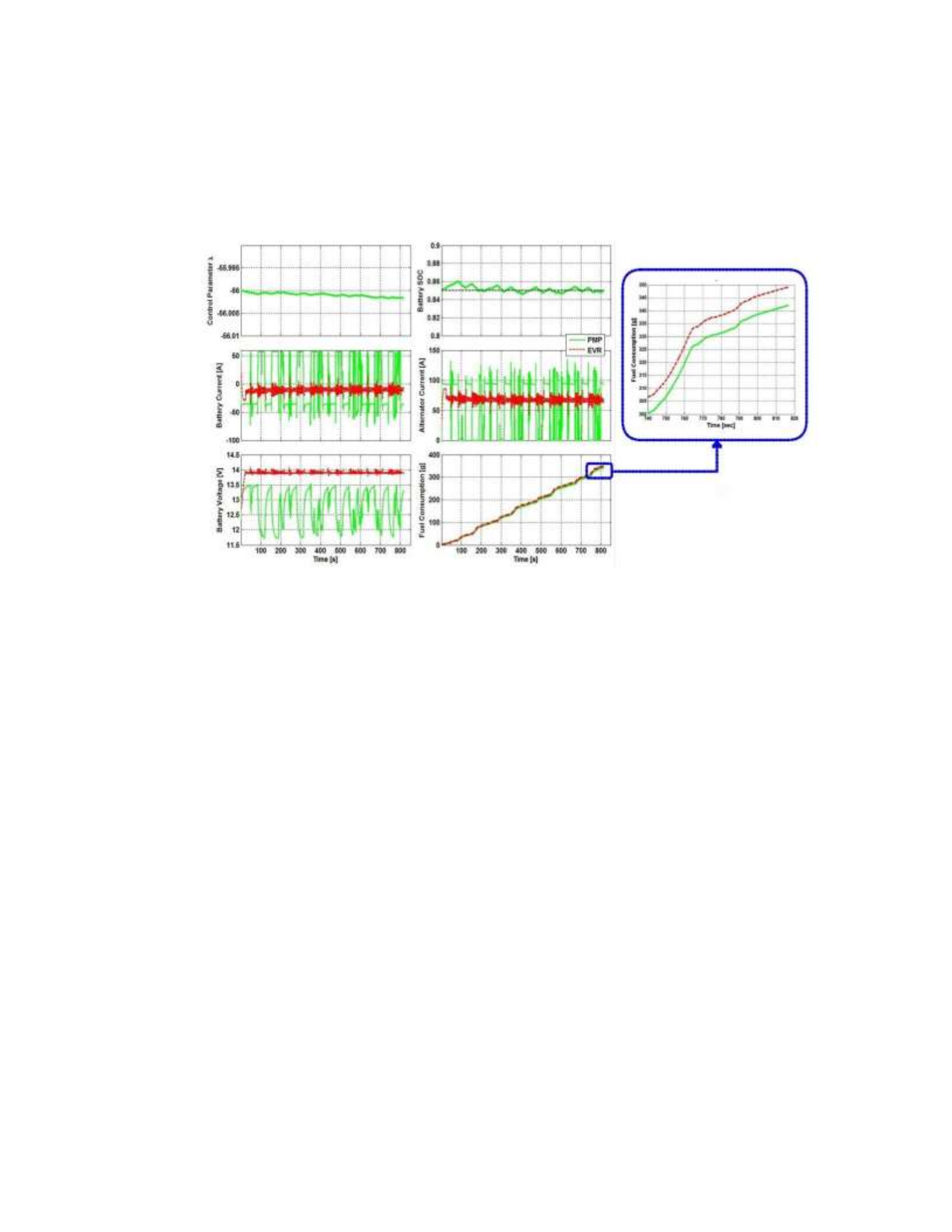
drive cycle. The behavior of the vehicle electrical system, instantaneous fuel
consumption, and co-state dynamics may be observed in Figure 39.
Figure 39: Results of Optimal Control Case Study
The co-state dynamics of the electrical load and driving schedule under consideration,
depicted in the upper left corner of Figure 39, are essentially non-existent, varying by less
than 0.01% over the entire length of the drive cycle. This trend is not isolated to this
particular case study, and is rather observed in all scenarios considered (refer to Table 7).
The variety of driving schedules and load profiles considered is discussed in greater detail
in Section 3.2.4. The charge-sustaining behavior of the battery may be verified in the
upper right corner of Figure 39, as the final state of charge is equal to the initial state of
charge; 85%. This reference SOC was predetermined based on experience, and will be
discussed in more depth in Section 3.2.3. The second row of plots in Figure 39 shows

64
both the battery and alternator current profiles for the VES subjected to the baseline EVR
controller and the PMP optimal control strategy. Of particular interest is the current
commanded to and from the battery. While the EVR maintains a nominal charging
current of approximately 15A in order to sustain the battery at the appropriate reference
voltage, the PMP control strategy allows for the battery to be used as a dynamic energy
storage device, with current values ranging from approximately -65A to 50A. The
primary driver for these fluctuations between positive and negative current may be
observed in Figure 40.

65
Figure 40: Optimal Control Case Study: Cause of Battery Current Fluctuations
An increase in the vehicle’s instantaneous fuel mass flow rate results in an increase in the
battery current, corresponding to a battery discharge event. Keeping in mind Equation 33,
the underlying reasons for this are evident. As the instantaneous fuel consumption of the
vehicle increases, the apparent value of the battery energy imposed by the co-state
variable diminishes in comparison. This translates to a de-weighting of the chemical
energy contained within the automotive battery, ultimately resulting in battery discharge.
As the fuel mass flow rate begins to drop off, the influence of the co-state variable
increases, resulting in a battery charging event. It is interesting to compare both the
battery current and vehicle velocity profiles; heavy acceleration events are accompanied
by electrical assistance from the battery (as supplied to the loads), whereas coasting and
braking events are associated with battery charging. This type of behavior is quite similar

66
to regenerative braking schemes, where inertial energy otherwise lost to the atmosphere
via an automobile’s braking system may be recuperated by an electric machine. The lower
left plot in Figure 40, which shows the battery voltage of the VES subjected to the EVR
and PMP, assists in illustrating the dynamic behavior of the optimally controlled electrical
system, and the importance of the imposed system constraints. The lower right plot in
Figure 40 compares the vehicle fuel consumption of the EVR and PMP control strategies.
The cumulative difference in fuel consumption between both control strategies results in a
2.1% improvement in fuel economy with optimal control. Table 5 provides the details of
the overall fuel economy benefits realized with optimal control.
Table 5: Optimal Control Case Study: Fuel Economy Improvement
Controller
Fuel Economy (mpg)
Chrysler EVR
19.1
Optimal Control
19.5
% Improvement
2.1%
3.2.3: Control Parameter Sensitivity Analyses
In order to determine the most suitable control parameters, evaluate the robustness of the
control strategy, and develop an implementable VES control strategy adapted from
optimal control theory, numerous sensitivity analyses are performed. These analyses are
performed for the same driving schedule and electrical load profile considered in Section
3.2.2. First, an analysis focusing on the resilience of the VES and PMP controller to errors
in the selection of the optimal initial condition for the co-state variable is performed. The
effects of changing the reference battery state of charge on fuel economy and VES model
behavior are then studied, followed by an investigation into the effects of modifying the
67
electrical system constraints. Finally, as the PMP controller subjects the battery to much
more rapid and higher magnitude current swings than does the EVR, the cumulative
energy flux of the battery for the control scenario is evaluated.
The ability of the controller to cope with sub-optimal control parameters is imperative in
developing any sort of implementable control strategy, as the online controller will never
have knowledge of a given drive cycle and VES load profile beforehand and can therefore
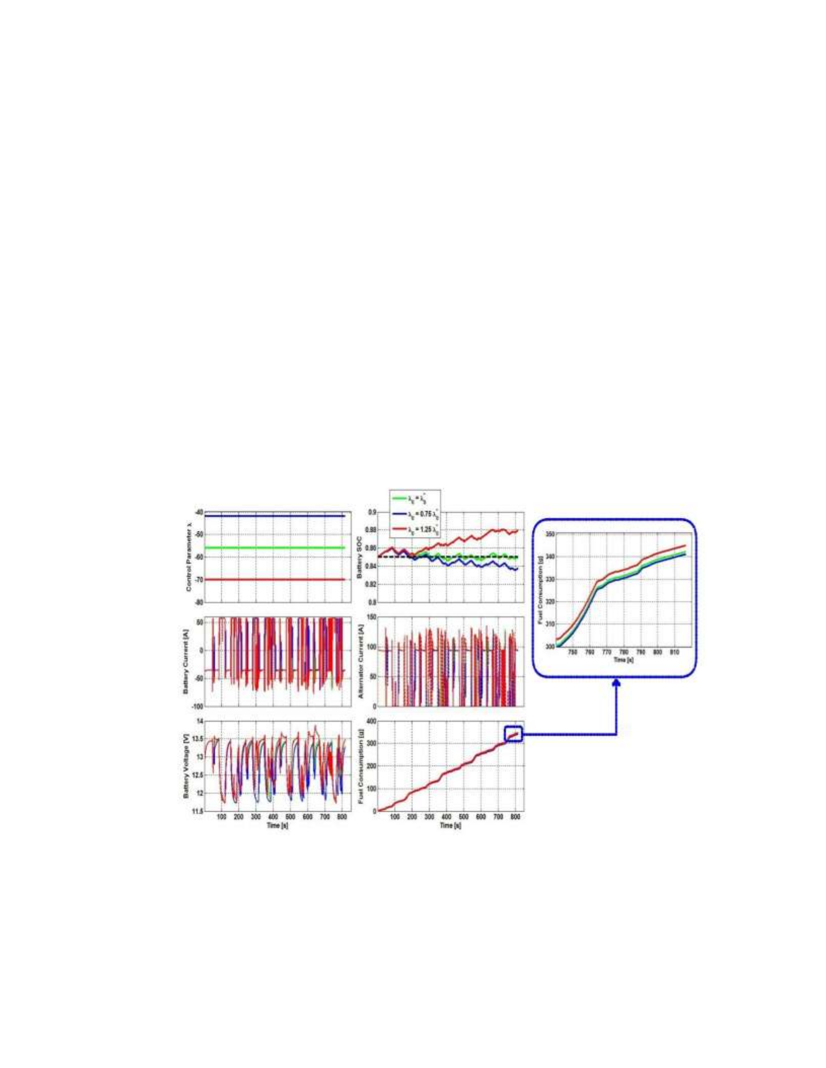
only estimate an, almost assuredly sub-optimal, co-state value. In order to study the
effects of sub-optimal co-state values, the VES model (subjected to PMP control) is
simulated with co-state values of +/-25% of the optimal solution. The results of this
study are featured in Figure 41.

68
Figure 41: Co-State Sensitivity Analysis
Upon observation of the upper right plot in Figure 41, it is clear that underestimating the
initial co-state value by 25% results in a discharge of approximately 1% battery SOC; only
1/3 of the way towards the lower threshold on the battery state of charge (82%). In
contrast, by overestimating the initial co-state value by 25% the battery SOC drifts to the
upper SOC threshold (88%) in approximately 700 seconds. If the co-state variable is
overestimated, the duty-cycle command sent to the alternator is less likely to result in
battery discharge. On the other hand, if the co-state variable is underestimated, battery
charging events are less likely to occur as the value of the battery energy (determined via
the co-state variable) is small in comparison with the value of the fuel energy. These
results demonstrate that in order to develop any sort of implementable, real-time control
strategy, there is a need for control adaptations which prevent the relatively slow battery
SOC drift resulting from a sub-optimal initial co-state value.
The battery reference state of charge holds particular relevance in terms of control
optimality as the battery should ideally operate around the reference SOC value for its
entire lifespan. An effort should therefore be made to understand the impact of the
reference state of charge on VES behavior and fuel economy. In order to do so, the
reference battery SOC (and the corresponding upper and lower SOC thresholds) is held to
three values: 85%, 90%, and 92.5%. The state of charge of the battery should not be
increased much above 92.5% as the internal resistance of the battery increases
dramatically at near 100% SOC values, therefore decreasing charge acceptance [23].
Likewise, the battery SOC should also not be decreased much below 80% due to both the

69
concern of sufficient current draw for engine startup, and the risks inherent in lead-acid
battery deep cycling (as discussed in Section 2.3.2)
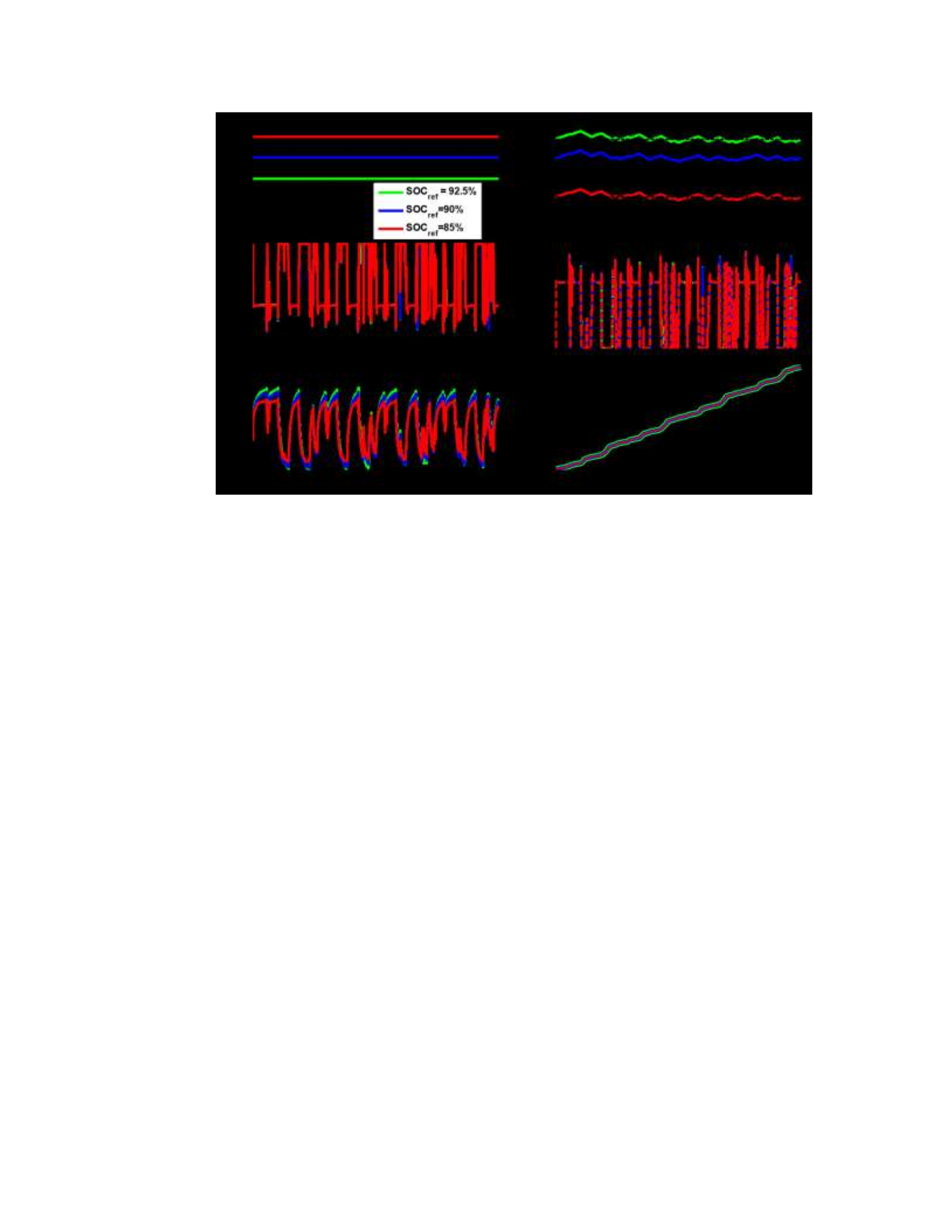
The results of the reference state of charge analysis are depicted in Figure 42 below.
70
Figure 42: Reference Battery State of charge Sensitivity Analysis
It may be observed that only trivial differences exist, both in terms of VES behavior and
the optimal co-state value, upon varying the reference state of charge and corresponding
upper and lower SOC bounds. What is notable, however, is the slight increase in both the
co-state variable and the magnitude of battery voltage swings as the reference SOC is
increased. This may be explained by the fact that the battery model internal resistance
increases as the battery state of charge increases from 85% to 92.5%. Despite battery
operation being slightly less efficient as the reference SOC is increased (via ohmic losses
in the equivalent circuit model), the corresponding decrease in fuel economy is negligible,
equating to less than 0.01% of the total vehicle fuel consumption. The reference battery

71
state of charge is therefore held to 85% in order to ensure that both deep-cycling and high
SOC operation need not be of concern.
The system constraints of the PMP controller, as discussed in Section 3.1.2, restrict the
dynamics of the vehicle electrical system in order to ensure customer comfort and safety,
and avoid excessive wear and tear on the battery and alternator. Restricting the VES
dynamics also translates to removing a number of potential candidates from the
currentsplit array (γ), resulting in a departure from optimal control behavior. It is
therefore necessary to balance both the reduction in VES aging, and the corresponding
reduction in vehicle fuel economy, due to the imposition of the VES system constraints.
Both the battery voltage constraints, 𝑉𝑚𝑖𝑛 and 𝑉𝑚𝑎𝑥, and the battery voltage time rate of
change constraint, 𝑉𝑚𝑎𝑥 , are initially non-existent, leaving the VES model behavior
unconstrained. The constraints are then imposed in finite increments in order to study the
corresponding reduction in the range of battery operating conditions and fuel economy.
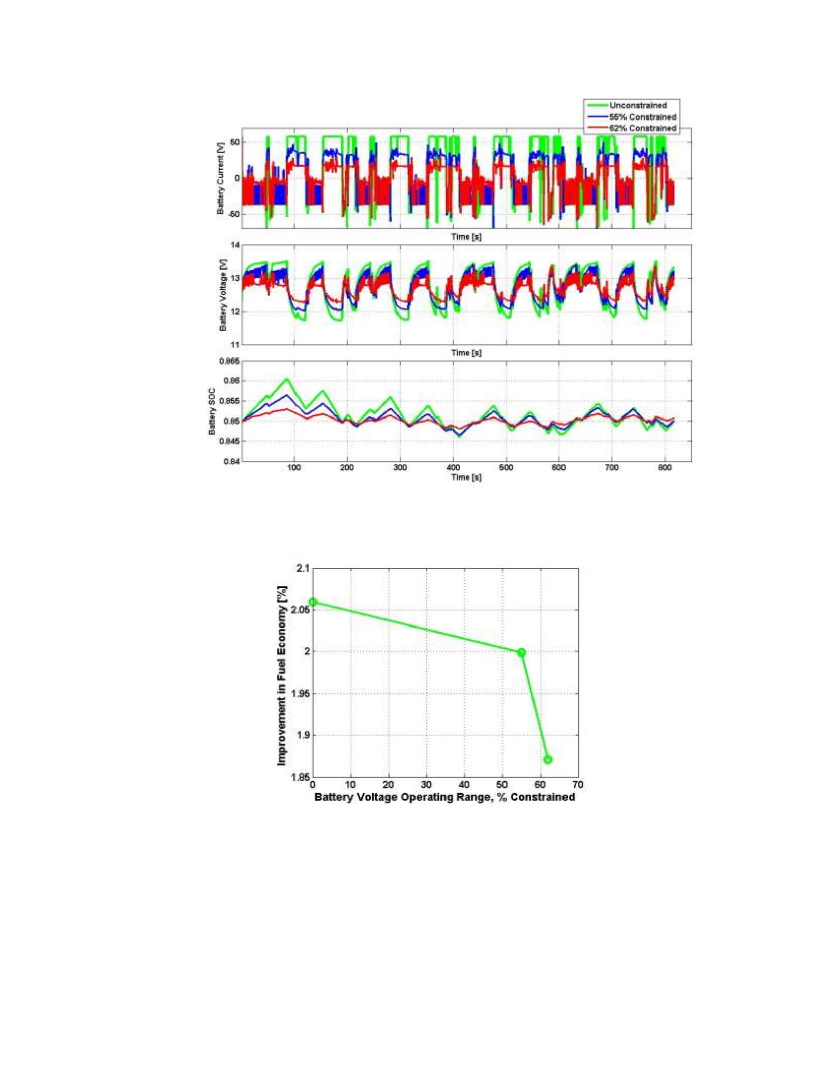
The results of the battery voltage constraint study are illustrated in Figures 43 and 44,
whereas the results of the battery voltage time rate of change constraint study are
depicted in Figures 45 and 46. Take note that as a 0th-order battery model is used to
predict the resultant battery voltage of all current-split candidates and filter out any
candidates that result in constraint violations, error is introduced into the imposed
constraints. Therefore, instead of specifying an exact value for the minimum and
maximum allowable battery voltage and the maximum allowable battery voltage time
rate of change, the percent reduction in battery operating range is specified. The VES

72
behavior is evaluated for the unconstrained, 55%, and 62% constrained battery voltage
scenarios, and is evaluated for the unconstrained, 38%, and 75% constrained battery
voltage time rate of change scenarios.
73
Figure 43: Battery Voltage Constraints Sensitivity Analysis

74
Figure 44: Battery Voltage Constraints Sensitivity Analysis, Fuel Economy
Figure 45: 𝒅𝑽𝒎𝒂𝒙 Constraints Sensitivity Analysis

75
Figure 46: 𝒅𝑽𝒎𝒂𝒙 Constraints Sensitivity Analysis, Fuel Economy
Upon observation of Figures 43 and 44, it may be noted that the battery voltage constraints
impact the behavior of the VES significantly, whereas restricting the time rate of change
of the battery voltage does very little to change overall VES behavior. This is indicative
of the PMP controller’s behavior; while extended periods of battery charging and
discharging (translating to a wide battery voltage operating range) lead to the optimal
solution, the optimal magnitude of these charging and discharging events does not much
surpass approximately 50A (translating to a limited 𝑑𝑉𝑚𝑎𝑥 value). The 𝑑𝑉𝑚𝑎𝑥 constraint,
however, does provide the advantage of filtering out some of the bang-bang behavior
which is characteristic of the PMP optimal control strategy. Limiting the battery voltage
therefore restricts optimal VES behavior more drastically then does limiting the time rate
of change of battery voltage. Despite the drastic changes in battery voltage behavior due
to constraining 𝑉𝑚𝑖𝑛 and 𝑉𝑚𝑎𝑥, the battery voltage never drops below 11.5V, and never
raises above 14V, well within the allowable voltage operating range. It logically follows
that imparting constraints upon the minimum and maximum allowable battery voltage
results in a greater reduction in fuel economy than reducing 𝑑𝑉𝑚𝑎𝑥, which may be
observed in Figures 44 and 46. Restricting the battery voltage operating range by 62%
results in an approximately 10% reduction of the PMP fuel economy benefits, whereas
restricting 𝑑𝑉𝑚𝑎𝑥 by 75% only reduces the PMP fuel economy benefits by about 5%.
Therefore, in order to facilitate maximum fuel economy benefits while avoiding any
undue, choppy battery current behavior, the battery voltage operating range will be

76
minimally constrained, whereas the time rate of change of the battery voltage will be
constrained by 38% (balancing the “filtering” and fuel economy benefits of the 𝑑𝑉𝑚𝑎𝑥
constraint).
The battery is subjected to much higher magnitude charging and discharging current levels
when regulated by the PMP controller. In order to gather an understanding of the
significance of this and quantify the extent to which the battery is utilized as an energy
mover as compared to the EVR controller, the absolute net energy flux (in ampere-hours)
of the battery is analyzed for both the case of the EVR and PMP control strategies. This
analysis is expanded to all combinations of drive and electrical load profiles in Section
3.2.4. Table 6 summarizes the results of the energy flux analysis for the VES model
subjected to the New European Drive Cycle at 57.5A.
Table 6: PMP Energy Flux Analysis Results
Controller
Energy Flux (Ah)
Chrysler EVR
4.07
Optimal Control
9.93
% Increase
144%
Approximately 9.93 Ah, or 13.24% of the battery’s capacity, are moved in and out of the
battery model when subjected to the PMP control strategy, whereas only about 4.07 Ah are
moved through the EVR-subjected battery model. The battery is therefore utilized to a
much greater extent as an energy mover with the PMP control strategy in place. While

77
fuel economy benefits are realized as a result of this, the results also imply that the battery
subjected to the PMP controller will be overused (when compared to the baseline EVR
controller). Any adverse effects that this overuse may have on the battery should therefore
be analyzed as well.
3.2.4: Extension of Control Analysis to Numerous Data Sets
In Sections 3.2.2 and 3.2.3, the effects of the optimal control strategy on the VES model
were investigated for the case of the New European Drive Cycle with a fixed electrical
load of 57.5A. This allowed for an in-depth analysis in regards to the influence of
numerous control parameters (i.e. system constraints, initial co-state value, etc…) on VES
behavior and fuel consumption. In order to fully understand how the optimal control
strategy functions over a wide variety of operating conditions, this analysis is expanded to
numerous combinations of driving cycles and constant electrical load profiles. By fixing
the electrical load to a constant value and varying the driving schedule, the effects which
the driving schedule and electrical load demand have on the determination of the optimal
control and state trajectories may be essentially decoupled from one another and studied
independently. This process is critical to the development of an adaptive, implementable,
Pontryagin-derived control strategy, and is summarized as follows.
The optimal initial co-state value is first located for each individual drive-cycle/electrical
load combination. Simulations are then run for each optimal scenario considered, and the
improvement in fuel economy, overall change in battery state of charge(𝑆𝑂𝐶𝑓 − 𝑆𝑂𝐶0),
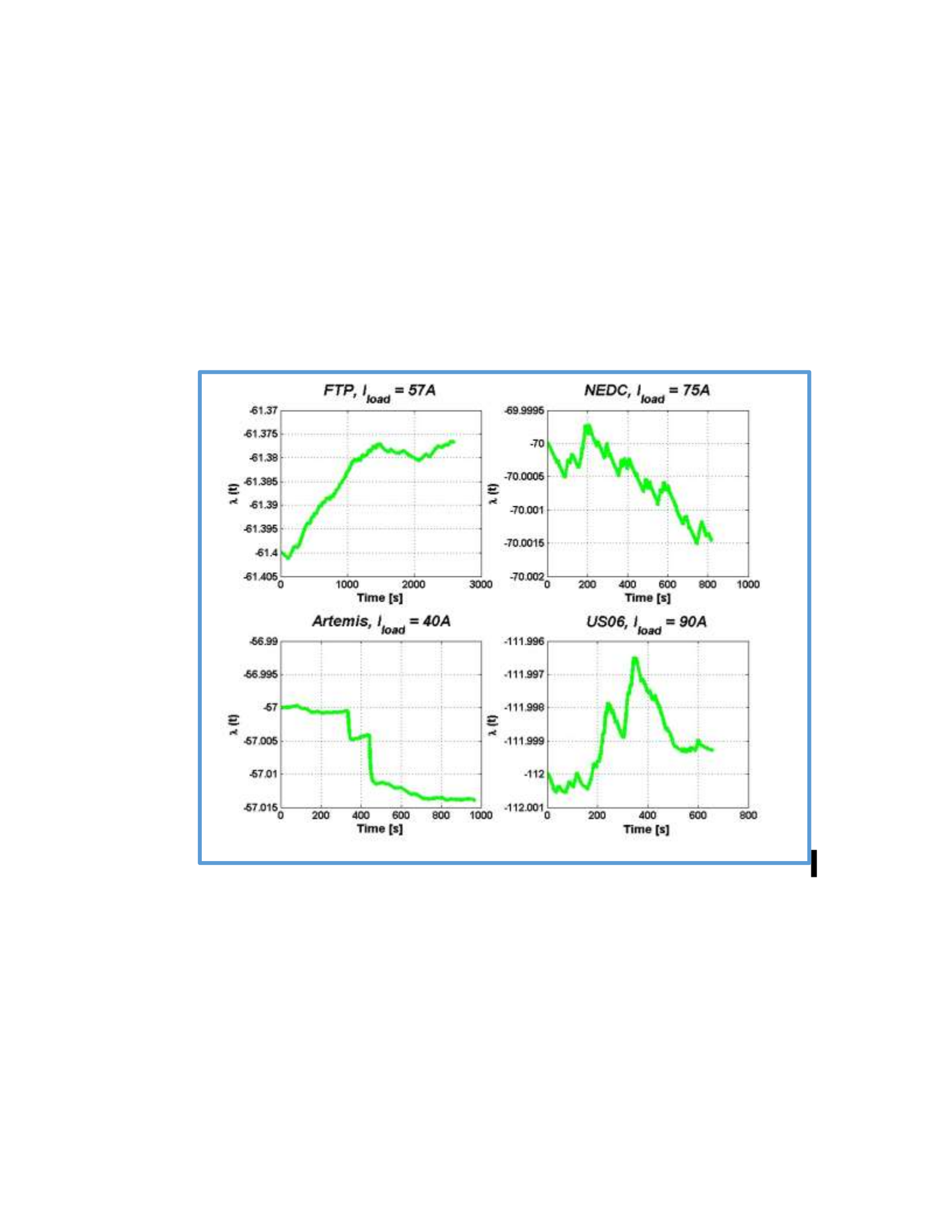
78
and net energy flux of the battery (in ampere-hours) are all tabulated. The battery SOC
trajectory for each control scenario considered is studied in detail to ensure that the upper
and lower state of charge bounds are not violated at any point during the drive cycle. The
co-state trajectory is observed as well in order to ensure that a near-constant value is
maintained over the length of the drive cycle under consideration. A representative set of
co-state dynamics extracted from simulation results may be observed in Figure 47.
Figure 47: Sample Set of Co-state Dynamics
The initial co-state value is then increased and decreased by 25%, and the resultant
improvement in fuel economy and change in battery SOC are tabulated as well. This

79
process is performed for a total of 35 different drive-cycle/electrical load combinations,
with the results featured in Tables 7-10. Take note that % F.E. denotes the percentage
improvement in fuel economy over the baseline EVR control strategy.
Table 7: Listing of Performance Parameters for PMP Controller
Load [A]
30
40
57.5
75
90
Drive Cycle
𝜆∗0
%𝐹. 𝐸.
𝜆∗0
%𝐹. 𝐸.
𝜆∗0
%𝐹. 𝐸.
𝜆∗0
%𝐹. 𝐸.
𝜆∗0
%𝐹. 𝐸.
FTP
-59
1.7
-61
1.7
-61
1.7
-80
1.8
-105
1.7
FTP (no soak)
-56
1.8
-62
1.7
-78
1.6
-90
1.6
-108
1.6
NEDC
-27
1.8
-28
1.7
-56
2.1
-70
2.2
-90
2.2
Artemis
-54
1.2
-57
1.2
-58
1.6
-77
1.7
-97
1.7
Indian Urban
-20
1.2
-57
1.6
-66
1.8
-76
1.9
-91
1.9
JC08
-49
1.5
-53
1.9
-68
1.8
-78
1.9
-100
1.7
US06
-60
0.6
-76
1.0
-89
1.1
-105
1.0
-112
1.0
It may be observed from Table 7 that the optimal control strategy consistently provides
improvements in fuel economy ranging from 0.6% all the way up to 2.2% in simulation.
Additionally, the boundary penalty function is set to a fixed value of 400 which is
sufficient, even in the case of an incorrect calibration of the initial condition of the
Lagrangian multiplier, as is the case in Tables 9 and 10. Of particular interest when
investigating the various optimal control scenarios featured in Table 7 is the relation
between the optimal initial co-state value, the driving cycle, and the electrical load
demand. At lower electrical load demands, there is a slight variance in the optimal initial
co-state value from drive cycle to drive cycle; particularly in regards to the NEDC and
Indian Urban drive cycles. However, as the electrical load demand is increased, the
variance in 𝜆0 from drive cycle to drive cycle diminishes, leaving the electrical load
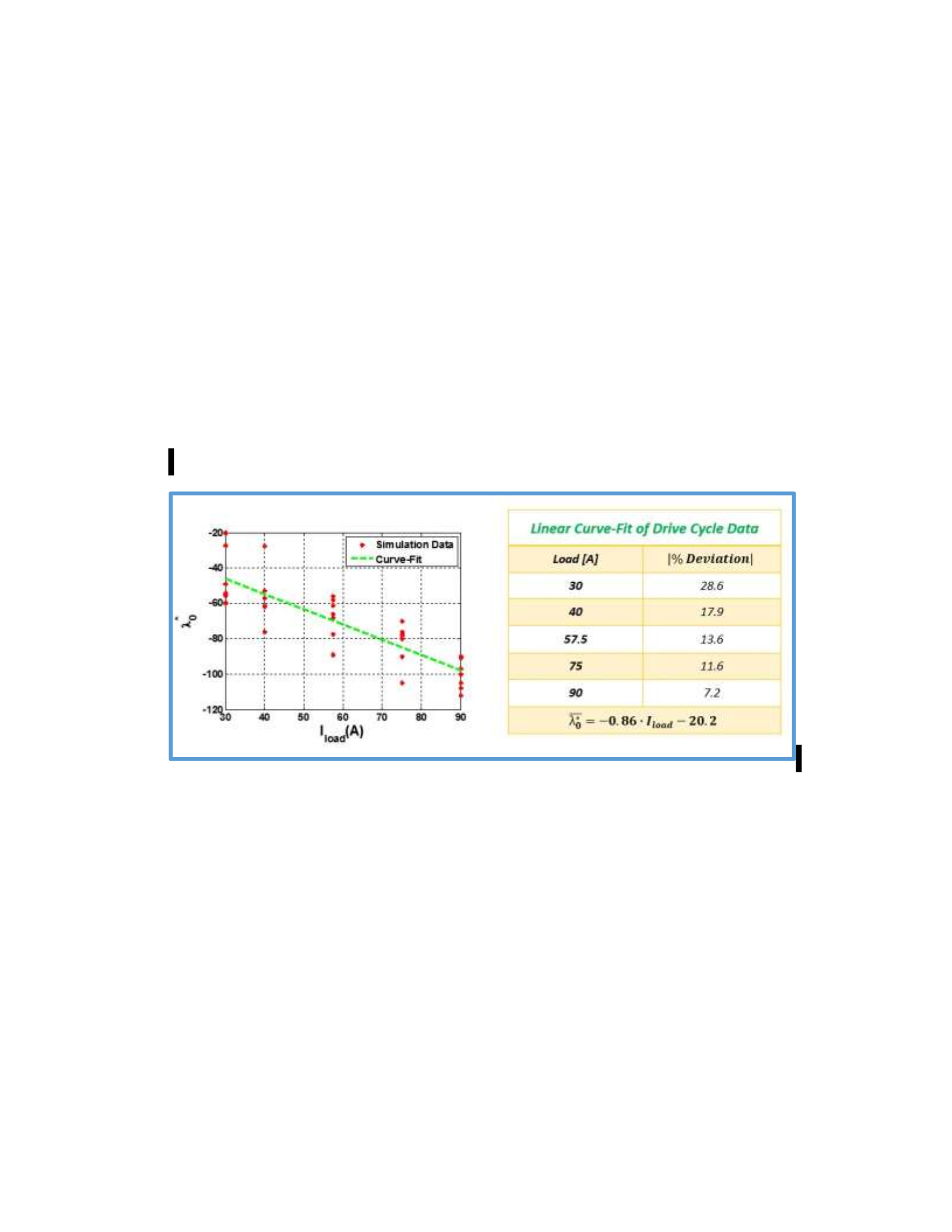
80
demand as the primary factor influencing the optimal initial co-state value. Furthermore,
as the actual vehicle electrical system will typically not see extended periods of usage
much below 60-70A of load, the co-state drive cycle variance at 30A and 40A of load is of
lesser importance than any variance at higher electrical loads. In an effort to quantify the
variance in the optimal co-state value at each constant electrical load scenario considered,
𝜆0 is plotted versus the electrical load demand for each drive cycle. All 35 data points,
one for each control scenario considered, are then linearly curve-fit. This process is
depicted in Figure 48.
Figure 48: Variance in Optimal Initial Co-state Value
The maximum percent deviation is simply the average percent difference between the
curve-fit and each data point, and may be observed to be approximately 28.6% at an
electrical load of 30A. As the electrical load is increased, this variance decreases; all the
way down to 7.2% at an electrical load demand of 90A. These findings prove to be
particularly significant and useful when developing an implementable PMP-based control
strategy, which will be discussed in Chapter 4.

81
Table 8: Additional Performance Parameters for PMP Controller (𝝀𝟎 = 𝝀∗𝟎)
Load [A]
30
40
57.5
75
90
Drive Cycle
∆𝑆𝑂𝐶
[%]
|𝛷𝐸|
[𝐴ℎ]
∆𝑆𝑂𝐶
[%]
|𝛷𝐸|
[𝐴ℎ]
∆𝑆𝑂𝐶
[%]
|𝛷𝐸|
[𝐴ℎ]
∆𝑆𝑂𝐶
[%]
|𝛷𝐸|
[𝐴ℎ]
∆𝑆𝑂𝐶
[%]
|𝛷𝐸|
[𝐴ℎ]
FTP
0.8
25.2
-0.1
31.3
0
32.0
0.3
26.7
-0.2
19.1
FTP (no soak)
-0.2
20.6
0.3
24.4
-0.3
24.4
0.3
22.2
0.1
16.8
NEDC
-0.5
7.6
-0.2
9.2
0.1
9.9
0
8.4
-0.2
5.3
Artemis
0.4
15.3
0.6
15.3
-0.4
12.2
-0.1
10.7
-0.2
6.9
Indian Urban
-0.2
15.3
-0.8
4.6
0
30.6
0.1
30.6
-0.3
20.6
JC08
-0.2
11.5
0.7
13.7
0.2
14.5
-0.2
12.2
-0.1
8.4
US06
0
4.6
-0.2
22.9
-0.2
9.2
0
8.4
-0.1
6.9
Referring to Table 8, two conclusions may be drawn regarding the optimal control
strategy; the net change in the battery state of charge is always maintained to below 1%,
and the net energy flux of the battery is typically many times greater than the EVR
battery energy flux. The most severe example of the difference in battery energy flux is
observed for the case of the FTP drive cycle at a fixed electrical load of 57.5A. At 32 Ah,
the amount of energy flowing in and out of the battery subjected to optimal control is
over 2.5 times greater than the energy flux of the battery when controlled by the EVR.
Table 9: Listing of Performance Parameters for PMP Controller
Load [A]
30
40
57.5
75
90
Drive Cycle
∆𝑆𝑂𝐶
[%]
%𝐹. 𝐸.
∆𝑆𝑂𝐶
[%]
%𝐹. 𝐸.
∆𝑆𝑂𝐶
[%]
%𝐹. 𝐸.
∆𝑆𝑂𝐶
[%]
%𝐹. 𝐸.
∆𝑆𝑂𝐶
[%]
%𝐹. 𝐸.

82
FTP
-2.8
0.9
-2.8
0.9
-2.9
0.7
-2.6
0.8
-2.7
0.8
FTP (no
soak)
-2.8
1.0
-2.8
0.9
-2.3
0.8
-2.5
0.8
-2.7
0.8
NEDC
-3.0
1.1
-3.0
1.0
-1.1
1.6
-2.9
2.1
-3.0
2.1
Artemis
-2.5
1.1
-1.8
2.0
-2.8
1.2
-2.6
1.4
-2.9
1.5
Indian
Urban
-3.0
0.8
-3.0
1.0
-2.6
1.0
-2.7
1.2
-2.9
1.2
JC08
-2.7
1.0
-2.7
0.8
-2.8
0.9
-2.8
1.0
-2.9
1.2
US06
-1.4
0.5
-3.3
0.7
-1.5
0.8
-2.4
0.9
-2.8
0.9
Table 9 demonstrates the effects of under-estimating the optimal initial co-state value by
25%. This under-estimation translates to a devaluing of the battery energy, resulting in
overall charge-depleting battery behavior. Despite excessive battery discharge, the fuel
economy is still largely negatively influenced by this sub-optimal control behavior. Take,
for instance, the percent improvement in fuel economy for the FTP drive cycle; at the
optimal initial co-state value the average improvement in fuel economy over all electrical
load scenarios considered is approximately 1.7%. In comparison, the average
improvement in fuel economy for the FTP drive cycle when the initial co-state value is
under-estimated by 25% is only about 0.7%.
Table 10: Listing of Performance Parameters for PMP Controller
Load [A]
30
40
57.5
75
90
Drive Cycle
∆𝑆𝑂𝐶
[%]
%𝐹. 𝐸.
∆𝑆𝑂𝐶
[%]
%𝐹. 𝐸.
∆𝑆𝑂𝐶
[%]
%𝐹. 𝐸.
∆𝑆𝑂𝐶
[%]
%𝐹. 𝐸.
∆𝑆𝑂𝐶
[%]
%𝐹. 𝐸.
FTP
3.0
0.5
3.0
0.5
2.6
0.6
2.2
0.6
3.0
0.2

83
FTP (no
soak)
3.0
0.6
3.0
0.5
3.0
0.3
3.0
0.3
3.0
0.2
NEDC
3.0
0.4
2.8
0.5
3.0
0.6
3.0
0.5
2.3
0.5
Artemis
3.0
0.4
1.9
0.2
3.0
0.5
3.0
0.4
3.0
0.2
Indian
Urban
3.0
0.4
1.7
0.7
3.0
0.8
3.0
0.8
3.0
0.7
JC08
3.0
0.4
2.9
0.3
3.0
0.1
3.0
0.2
3.0
-0.1
US06
0.1
0.3
3.0
0.2
3.1
0.3
3.0
0.1
3.0
0.0
Referring to Table 10, the fuel economy is observed to decrease drastically when the
costate variable is over-estimated by 25%. This may be attributed to two factors; the
control strategy is operating on a sub-optimal control and state trajectory, and the battery
is charged over the length of the drive cycle under investigation. A portion of the overall
reduction in vehicle fuel economy may therefore be associated with the fuel invested into
charging the battery.
By evaluating various combinations of control parameters, drive cycles, and constant
electrical load demands in Sections 3.2.3 and 3.2.4, the underlying structure of the PMP
control strategy is established. The critical observations and analyses performed in this
chapter may be summarized as follows:
• The state constraints and reference battery SOC are selected in order to balance the
benefits of improved fuel economy with the consequences of rapid battery current
swings and battery over-usage.
• The governing factors which determine the optimal control and state trajectories
are determined to be primarily functions of the initial co-state value, which in turn
depends heavily upon the electrical load demand of the VES.

84
• The dependence of the initial condition of the optimal co-state value on the driving
schedule diminishes as the electrical load demand increases.
• The co-state dynamics prove to be negligible, varying by as much as 0.01% in the
control scenarios under consideration.
These findings are all relied upon in Chapter 4 in order to develop an adaptive,
Pontryagin-based control strategy which may be implemented in a production vehicle in
real-time.

85
Chapter 4: Development and Implementation of an Adaptive-PMP Control
Strategy
In the previous chapter, an optimal control strategy was derived from Pontryagin’s
Minimum Principle for the energy-optimal control of the electrical system of a passenger
vehicle, and was verified in simulation. While this control strategy allows one to evaluate
the potential for fuel economy improvement, such benefits may not be realized without
all knowledge of the driving profile and electrical load profile “a priori”. Thus, there is a
need to modify the existing PMP control in order to allow for an online, or
“forward-looking” implementation, without “a priori” knowledge of the driving and load
profiles.
The present chapter bridges the gap between the optimal PMP control strategy and an
adaptive, PMP-based control strategy which is implementable in real time.
The chapter begins by highlighting the critical findings of Chapter 3 that are relevant to
the development of a real-time capable control strategy; in particular the dependence of
the optimal control trajectory on observable vehicle states and outputs (i.e. current,
voltage, etc…). These findings are then translated into a physical control structure which
replaces the co-state dynamics subsystem discussed in Section 3.1.3, thus removing the
need for “a priori” input knowledge. The adaptive control strategy (A-PMP) is then tuned
in simulation to yield the best possible fuel economy, and benchmarked against the PMP
control. Section 4.2 discusses the controller experimental test setup, and includes a
summary of experimental testing results with respect to vehicle fuel economy. Finally,

86
Section 4.3 addresses potential drivability issues associated with the A-PMP control
strategy and examines possible solutions to these problems with special consideration
given to vehicle fuel economy.
Section 4.1: Design of an Adaptive PMP-based Control Strategy
Proper tuning of the initial condition of the co-state variable, 𝜆0, is essential in determining
the optimal control trajectory with respect to both charge-sustaining behavior and minimal
fuel consumption. This condition is, however, contingent on the appropriate selection of
the initial condition of the co-state variable, which requires a priori knowledge regarding
the specific drive cycle and electric load profile of interest. Such a control strategy is non-
causal in nature, and would thus be impossible to implement in a forward-looking case.
Therefore, in order recognize any potential fuel savings in-vehicle, it is first necessary to
develop a control strategy that can approximate the co-state value with a separately
defined control parameter, which will be termed “lambda”, and update the value of this
parameter as needed to ensure charge-sustaining behavior and improve vehicle fuel
economy. The newly defined control parameter (𝜆) is passed into the Hamiltonian
calculation subsystem just as the co-state variable is in optimal control, and may be
expressed as follows.
𝜆(𝑘) = 𝐾𝑆𝑂𝐶 ∙ (𝑆𝑂𝐶(𝑇𝑠1) − 𝑆𝑂𝐶𝑟𝑒𝑓) + 𝜆0(𝑇𝑠2) (36)
Where 𝑘 is an integer number indicating the discrete time step, and 𝑇𝑠 denotes adaptations
made to the function at regular intervals of fixed duration. Take note that 𝑇𝑠1 and 𝑇𝑠2 do
not necessarily need to be equal to one another.

87
As discussed in Section 3.2.4, the co-state dynamics (w/ constant electrical loads imposed)
appears negligible throughout the entirety of each driving schedule considered and could
thus be approximated as constant and equal to its initial value. Table 8 illustrates the
dependence of the initial condition of the co-state variable on both drive cycle and
electrical load. While there is a notable, inversely proportional relationship between the
optimal initial condition of the co-state variable and the electrical load demand, the
dependence of 𝜆0 on the driving schedule decreases significantly as the electrical load
demand increases above 57.5A. As the radiator fan alone requires 30-40A and typical
operating conditions in the vehicle requires between 60-80A, the contribution of the
driving profile to the optimal initial condition of the co-state variable may be neglected for
implementation purposes. Following this point, the optimal initial condition of the co-
state variable may be approximated solely as a function of the electrical load demand.
Figure 48 quantifies the variance in the optimal initial condition of the co-state variable
with no consideration given to the driving schedule, only the electrical load demand. As
an example, at a load demand of 90A the percent deviation in the optimal initial condition
of the co-state variable between all 7 drive cycles considered is only 7.2%, justifying the
approximation of the initial condition of the co-state variable as a function of electrical
load demand alone. Therefore, the electrical load demand of the vehicle may be measured
in real time and passed through a lookup table in order to approximate the optimal initial
condition of the co-state variable. From this point onward, 𝜆0 refers to the output of this
lookup table and no longer to the initial condition of the co-state variable. The lookup
table was generated for electrical load values of 30A, 40A, 57.5A, 75A, and 90A by

88
averaging the corresponding optimal initial conditions of the co-state values across all
driving schedules considered in Section 3.2.4, with the exception of the NEDC and Indian
Urban drive cycle. The NEDC and Indian Urban drive cycles are ignored due to numeric
disparities with the rest of the initial conditions of the co-state variables (at low electrical
loads). Table 11 features the 𝜆0 lookup table as a function of electrical load.
Table 11: 𝝀𝟎 Lookup Table
𝑰𝒍𝒐𝒂𝒅 (𝑨)
𝝀𝟎(𝑰𝒍𝒐𝒂𝒅)
30A
-55.6
40A
-61.9
57.5A
-70.8
75A
-86
90A
-104.4
The 𝜆0 lookup table does not operate continuously in time, but rather is updated at discrete
sampling instances (𝑇𝑠2 = 𝑇𝑠(𝐼𝑙𝑜𝑎𝑑)). This provides for an educated projection of the
charge-sustaining control solution, however the battery state of charge will depart from the
reference value without an additional term incorporated into 𝜆.
A proportional correction on this “SOC-drifting” behavior, which is based on SOC
feedback and ensures the robustness of the control strategy [17], is necessary to ensure
that excessive battery depletion or charging does not occur. This approach towards
ensuring charge-sustaining battery behavior has been used in automotive control
applications with success, and may be investigated in greater detail in [31, 34]. From an
implementation perspective, the proportional correction on the battery state of charge may
be expressed as follows.

89
SOC Correction Factor = 𝐾𝑆𝑂𝐶 ∙ (𝑆𝑂𝐶(𝑘) − 𝑆𝑂𝐶𝑟𝑒𝑓) (37)
Where 𝐾𝑆𝑂𝐶 is the proportional gain on the differential of the battery state of charge,
𝑆𝑂𝐶(𝑘) is the actual battery state of charge, and 𝑆𝑂𝐶𝑟𝑒𝑓 is the reference battery state of
charge. The corrective term on the battery state of charge is updated at discrete sampling
times (𝑇𝑠1 = 𝑇𝑠(∆𝑆𝑂𝐶)), in order to allow the vehicle to make use of the available energy
buffer. The SOC-correction is added to the output of the 𝜆0 lookup table, and the resulting
sum (alongside the average of the previous two lambda values) is taken as an input into
the Hamiltonian calculation subsystem.
Figure 49 assists in visualizing the underlying control logic of the newly defined
“Lambda-Calculation Subsystem”, which replaces the co-state dynamics subsystem of the
previously discussed PMP control. Take note that the electrical load demand is passed
through a moving average subsystem which filters the signal prior to the 𝜆0 LUT. The
purpose of the filter is to mitigate the high-frequency noise inherent in the battery and
alternator current measurements and allow for an approximation of the appropriate
lambda value based on the mean electrical load demand.
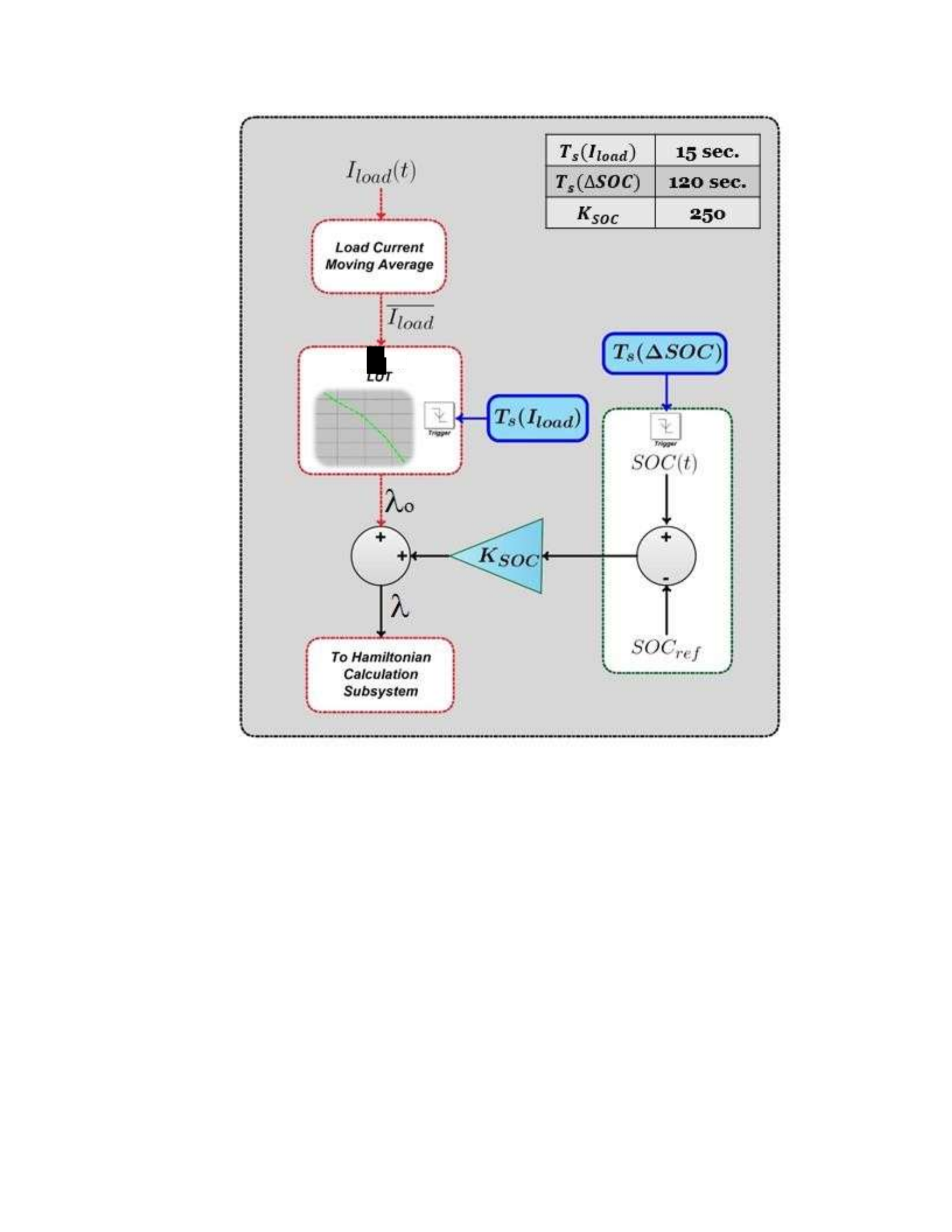
90
Figure 49: Lambda Estimation Control Structure
The gain on the battery state of charge, 𝐾𝑆𝑂𝐶, needs to be calibrated to ensure proper
weighting of the battery energy at both the upper and lower state of charge thresholds. In
particular, the net lambda value (i.e. the sum of the LUT and the SOC-correction) must
assist in maintaining the battery SOC around the reference value while still allowing
freedom for the battery to operate as an energy mover. If, for example, 𝐾𝑆𝑂𝐶 is set to too
𝜆
0

91
large a value, the battery SOC dynamics will be restricted and fuel economy benefits may
be significantly reduced. On the hand, if 𝐾𝑆𝑂𝐶 is set to a very small value, the battery SOC
will eventually drift to either the upper or lower threshold value, chattering for the
remainder of the drive cycle and reducing potential fuel savings. Proper calibration of the
proportional gain on the battery state of charge is therefore critical to the successful
implementation of an adaptive-PMP control strategy. In order to quantify the effects of
changing the SOC-gain and ensure that the best possible value is selected, the influence of
𝐾𝑆𝑂𝐶 on the trajectory of the battery state of charge and overall vehicle fuel economy must
be studied. The magnitude and frequency of the low frequency state of charge trajectory
are useful metrics in understanding how changes in the SOC-gain effect battery behavior.
Figure 50 illustrates how the SOC magnitude and frequency are determined, and features
simulation data derived from an on-road drive cycle. Take note that prior to any
calculation of the SOC magnitude and frequency, the state of charge signal is filtered to
remove dynamics with a frequency greater than 0.1Hz. This filter is implemented, strictly
in post-processing, to allow for accurate calculation of the “peak-to-valley” SOC values
(i.e. the SOC magnitude) and the “peak-to-valley” time intervals (i.e. the inverse of the
SOC frequency).
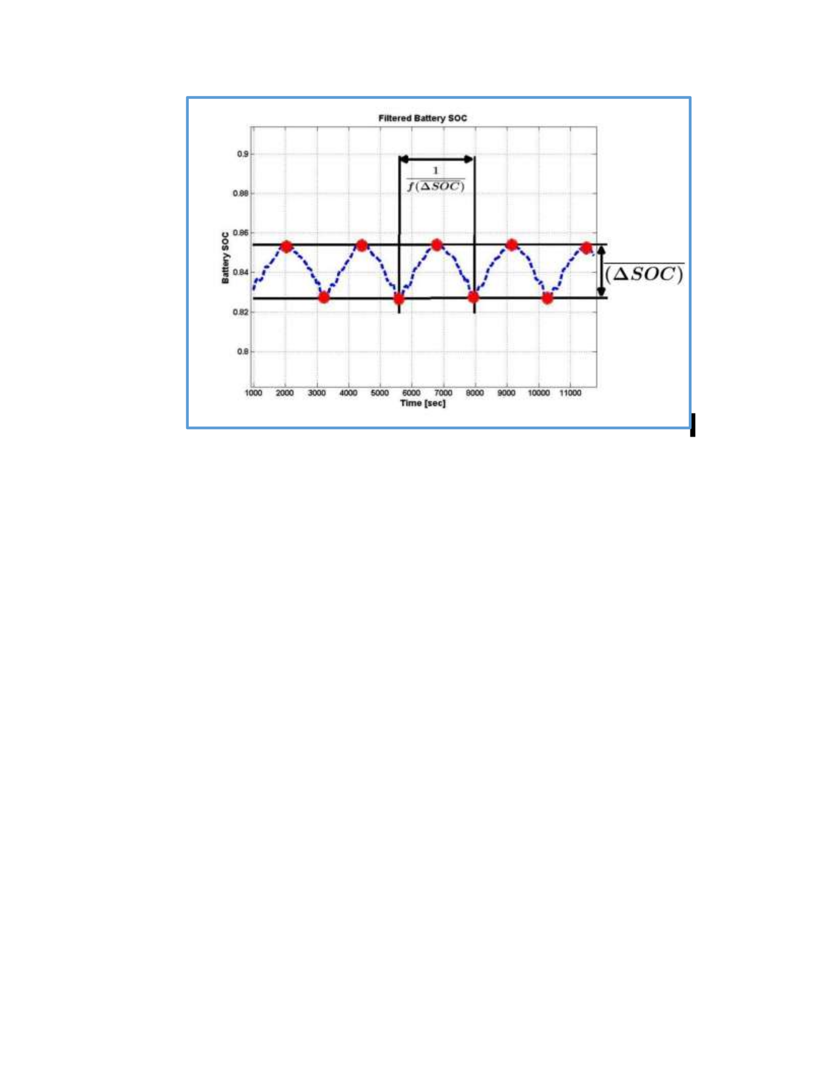
92
Figure 50: Metrics Used to Quantify State of charge Dynamics
Each SOC peak (maximum) and valley (minimum) is determined and marked, as observed
in Figure 50. The mean SOC “swing magnitude”, ∆𝑆𝑂𝐶, and the SOC “swing frequency”,
𝑓(∆𝑆𝑂𝐶), are then calculated by averaging the sum of the individual parameter values.
Table 12 catalogues the effects, in simulation, of changing 𝐾𝑆𝑂𝐶 on the aforementioned
SOC metrics, as well as fuel economy, over an on-road experimental drive cycle with
experimental electrical loads. This drive cycle, analyzed in simulation, will be the basis
for all control parameter tuning for the remainder of Section 4.1. Take note that the
rightmost column of Table 12 quantifies the ratio of the improvement in fuel economy w/
the adaptive control in place over the improvement in fuel economy w/ optimal control in
place (i.e. %F.E.*).

93
Table 12: Effects of Modifying SOC Gain
𝑲𝑺𝑶𝑪
∆𝑺𝑶𝑪 [%]
𝟏
[𝒔𝒆𝒄]
𝒇(∆𝑺𝑶𝑪)
%𝑭. 𝑬.
%𝑭. 𝑬.∗
100
6
1143
0.93
250
5.6
1180
0.94
500
5.2
1173
0.93
1500
4.2
1144
0.92
3000
2.6
2473
0.89
As 𝐾𝑆𝑂𝐶 is increased from 100 to 3000, ∆𝑆𝑂𝐶 decreases by approximately 57%. At a
value of 100, the battery is making use of the entirety of its SOC operating range (+/- 3%
SOC), and even saturates at the threshold values. In comparison, when 𝐾𝑆𝑂𝐶 = 3000, the
battery is using less than half of its allowable capacity. This behavior is to be expected,
as increasing the SOC-gain results in more charging at low SOC values and more
discharging at high SOC values, therefore discouraging SOC fluctuations. The period of
the SOC swings increases significantly when the gain is elevated from 1500 to 3000 due
to the restriction imposed on the battery dynamics. As the battery is forced to operate
within a very limited range of SOC values, “peaks” and “valleys” in the state of charge
are less likely to occur. Increasing the gain on the SOC differential has adverse effects on
the fuel economy due to more stringent limitations on the state of charge dynamics. The
battery is therefore not used to its fullest potential as an energy buffer. At an SOC-gain
value of 250, the fuel economy benefit provided by the adaptive control strategy is only
6% less than what optimal control provides. In contrast, when 𝐾𝑆𝑂𝐶 = 3000 , the
adaptive controller provides 11% less fuel economy benefit than the optimal control. A

94
tradeoff is therefore associated with selecting a value for 𝐾𝑆𝑂𝐶; too high of a value results
in diminished fuel economy benefits due to restrictions on battery usage, whereas too low
of a value potentially results in the battery reaching the SOC thresholds, thus also
reducing vehicle fuel economy (as shown in Table 12 for 𝐾𝑆𝑂𝐶 = 100). A SOC-gain of
250 provides maximum fuel economy while also preventing the state of charge from
reaching either the upper or lower allowable value, and is therefore selected for
implementation in the vehicle.
Referencing Figure 49, both the 𝜆0 lookup table and the proportional gain on the state of
charge differential include update times; 𝑇𝑠(𝐼𝑙𝑜𝑎𝑑) and 𝑇𝑠(∆𝑆𝑂𝐶), respectively. The
update time on the 𝜆0 LUT, 𝑇𝑠(𝐼𝑙𝑜𝑎𝑑), physically operates by sampling the moving average
of the electrical load signal at specified time intervals (𝑇𝑠) and holding the sampled value
in between sampling instances. This provides the functionality of smoothing out the
dynamics of 𝜆, and must be tuned in order to capture the true electrical load behavior. If
the sampling time is too large, major changes in the electrical load (such as what may be
introduced by switching on the cabin blowers or radiator fan) could potentially be
neglected due to the presence of the moving average filter, resulting in non-representative
values of 𝜆0. Thus, it is necessary to select a suitable value for 𝑇𝑠(𝐼𝑙𝑜𝑎𝑑) which can take
into account any significant changes in electrical load behavior while also mitigating
erratic co-state behavior. Table 13 catalogues the effects which

95
𝑇𝑠(𝐼𝑙𝑜𝑎𝑑) has on the battery SOC and vehicle fuel economy. In addition, the RMS error,
𝑒𝑅𝑀𝑆(𝐼𝑙𝑜𝑎𝑑), of the filtered electrical load signal as compared to the actual electrical load is
tabulated for reference.
Table 13: Effects of Modifying 𝑻𝒔(𝑰𝒍𝒐𝒂𝒅)
𝑻𝒔(𝑰𝒍𝒐𝒂𝒅) [sec]
𝒆𝑹𝑴𝑺(𝑰𝒍𝒐𝒂𝒅) [sec]
∆𝑺𝑶𝑪 [%]
%𝑭. 𝑬.
%𝑭. 𝑬.∗
15
6.87
5.4
0.93
60
9.17
5.8
0.93
120
11.09
5.9
0.89
180
12.75
6.0
0.89
The RMS error of the filtered electrical load signal increases as the sampling period
increases, translating to a less representative value for 𝜆0, and resulting in excessive
drifting of the battery state of charge from the reference value. At a sampling period of
180 seconds, the magnitude of SOC swings is equal to the allowable operating range of
the battery. In addition, as 𝑇𝑠(𝐼𝑙𝑜𝑎𝑑) is increased from 60 seconds to 120 seconds, the fuel
economy benefit decreases from 93% to 89%, largely due to the battery SOC reaching the
operating limits of the battery state of charge. While allowing the battery to make full use
of its SOC operating range proves beneficial to vehicle fuel economy, any time the battery
spends operating at the upper and lower threshold values has adverse effects on fuel
economy. Therefore, as a preventative measure, 𝑇𝑠(𝐼𝑙𝑜𝑎𝑑) is selected such that battery
operation around the upper and lower allowable SOC values is kept to a minimum, while
still allowing for an accurate calculation of the 𝜆0. A sampling period of

96
15 seconds satisfies both criteria, and is therefore deemed suitable for vehicle
implementation.
The update time for the gain on the SOC differential, 𝑇𝑠(∆𝑆𝑂𝐶), is necessary to allow the
controller to function more freely within the batteries allowable operating range (and thus
closer to the optimal control command). For example, with 𝑇𝑠(∆𝑆𝑂𝐶) set to a very low
value, as would be the case if 𝑇𝑠(∆𝑆𝑂𝐶) = 𝑇𝑠(𝐼𝑙𝑜𝑎𝑑), a significant departure from the
optimal control command will occur in proximity of the SOC thresholds due to the
heavily weighted additional term introduced by 𝐾𝑆𝑂𝐶. A portion of the batteries operating
range may therefore be under-utilized, resulting in diminished fuel economy benefits. In
comparison, a very large value for 𝑇𝑠(∆𝑆𝑂𝐶) tends to neglect SOC-drifting and
potentially allow the battery state of charge to reach the upper or lower allowable SOC
values, resulting in undesirable SOC chattering and again reducing the potential fuel
economy benefits that may be realized with such a control strategy. From a physical
standpoint, 𝑇𝑠(∆𝑆𝑂𝐶) is implemented by sampling the actual battery state of charge at
predefined time intervals, and holding this SOC value between sampling instances. A
study into the behavior of the A-PMP control strategy subject to various values of
𝑇𝑠(∆𝑆𝑂𝐶) is featured in Table 14.
Table 14: Effects of Modifying 𝑻𝒔(∆𝑺𝑶𝑪)
𝑻𝒔(∆𝑺𝑶𝑪) [sec]
∆𝑺𝑶𝑪 [%]
%𝑭. 𝑬.
%𝑭. 𝑬.∗
30
5.2
0.91
60
5.3
0.91
120
5.5
0.93

97
180
5.7
0.93
As the sampling time for the SOC-gain is increased from 30 to 180 seconds, ∆𝑆𝑂𝐶
increases from approximately 86% to 95% of the operating range of the battery. The
resulting fuel economy ratio reflects this, increasing from 91% to 93%. Similar to the
selection process laid out for 𝑇𝑠(𝐼𝑙𝑜𝑎𝑑), the sampling time for the state of charge gain is
chosen in order to balance fuel economy benefits with the potential ramifications of
allowing the state of charge to drift into either the upper or lower threshold. A sampling
time of 120 seconds proves to satisfy the desired performance criteria, and is therefore
selected for implementation in the vehicle. Table 15 summarizes the control parameters
selected for in-vehicle implementation
Table 15: A-PMP Control Parameter Selection Summary
Control Parameter
Value
𝑲𝑺𝑶𝑪
250
𝑻𝒔(𝑰𝒍𝒐𝒂𝒅)
15
𝑻𝒔(∆𝑺𝑶𝑪)
120
It may be observed from Tables 12-15 that the adaptive control strategy yields fuel savings
ranging from approximately 89-94% of the results provided by the optimal control for the
experimental drive cycle under consideration, with the primary drivers of these disparities
relating to the introduction of an approximation of co-state dynamics and in the model
describing the variation of the control parameter 𝜆0. The effects of these approximations
are not strictly limited to fuel economy, but alter the control trajectory, and thus VES
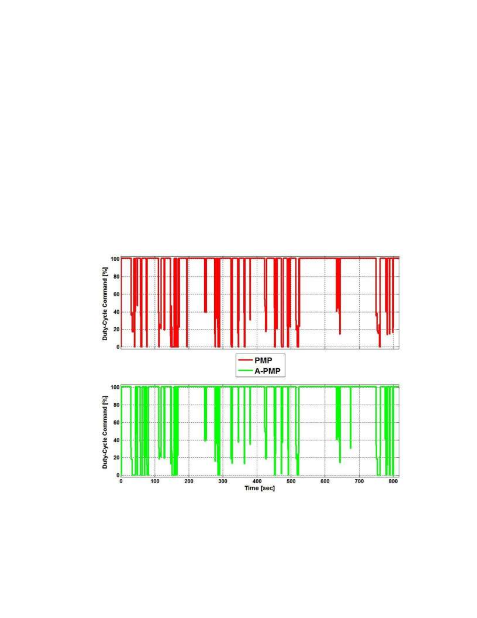
98
behavior, as well. In particular, any departure from optimal control will result in a change
in the duty-cycle command and the battery state of charge trajectory.
With minimal fuel economy differences observed between optimal control and the APMP
control strategy, it is reasonable to expect that the A-PMP control and SOC trajectories
will resemble those resulting from optimal control. Figure 51 depicts the control
command trajectories for both optimal control and the A-PMP control strategy. Figure 52
illustrates the similarities between the optimal control and A-PMP state of charge
dynamics over the first 815 seconds of the aforementioned experimental drive cycle.
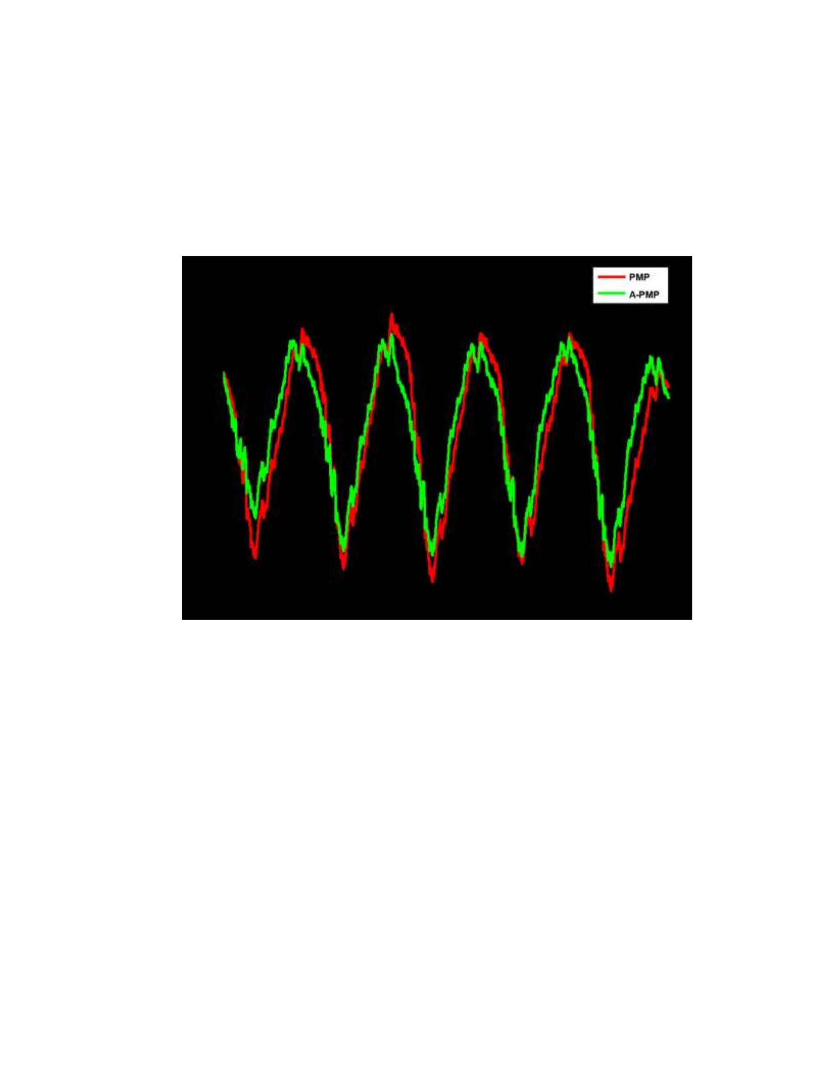
99
Figure 51: Comparison of PMP and A-PMP Control Command Trajectories
Referencing Figure 51, the A-PMP control command is observed to closely follow the
optimal control command.
State-of-Charge Dynamics for Experimental Drive Cycle
Figure 52: Comparison of PMP and A-PMP Battery SOC Dynamics
Figure 52 depicts the similarities between the optimal control and adaptive control state of
charge dynamics. The final battery state of charge of both the PMP and A-PMP control
strategies lie within half of a percentage of the initial SOC, indicating that the adaptive
control strategy provides suitable estimations of the co-state variable throughout the
entirety of the drive cycle under consideration. The battery subjected to the adaptive

100
control strategy is, however, observed to function within a smaller SOC operating range,
primarily due to the imposition of the state of charge corrective factor, 𝐾𝑆𝑂𝐶. As the
battery SOC diverges from the reference trajectory, the effects of the SOC correction
become more apparent (as may be noted in the “valleys” of the battery SOC).
Nonetheless, the adaptive control strategy provides near-optimal fuel economy
improvements, and results in control command and SOC trajectories which are very
similar to that resulting from optimal control. To ensure acceptable adaptive-control
performance across a wide variety of driving styles, the A-PMP controller is benchmarked
in simulation against the PMP control strategy with 3 additional experimental data sets.
The results of this analysis are featured in Table 16. Take note that the data set analyzed
throughout this section is titled “On-Road (08/30) x5”. Take note that “(08/30)” refers to
the date of experimental testing, and is used to differentiate the two different experimental
drive cycles considered in this section.
Table 16: Benchmarking of A-PMP against Optimal Control in Simulation
Drive Cycle
% 𝑭. 𝑬.
% 𝑭. 𝑬.∗
On-Road (08/30) x5
1.2
1.3
On-Road (09/06) x5
1.1
1.1
FTP x5
1.6
1.7
NEDC x5
1.5
2.0
The adaptive PMP control strategy consistently provides near-optimal fuel economy
improvements, despite the lack of “a-priori” velocity and electrical load profile
information. Furthermore, the battery SOC is maintained within the desired operating
range, avoiding any concern of excessive battery charging or discharging. This control

101
strategy is therefore suitable for real-time control, and may be directly implemented
invehicle.
Section 4.2: Implementation and Experimental Testing of the A-PMP
Control Strategy
In order to facilitate timely controller implementation and tuning, an ETAS ES1000.3
rapid prototyping platform is utilized for experimental testing. Detailed information
regarding the underlying hardware and software of the ETAS system is described and
illustrated in Section 2.1.2. Intecrio Experiment Environment software, operating on an
in-vehicle laptop computer, enables real-time controller tuning and vehicle behavioral
analysis, and allows for data acquisition as well. Experiment Environment also has the
added benefit of allowing the user to ensure that individual control subsystems and all
sensors coupled to the ETAS platform are functioning appropriately. Figure 53 illustrates
the Experiment Environment user interface during experimental controller testing.

102
Figure 53: Intecrio Experiment Environment User Interface
As discussed in Section 2.1.2, both a battery and alternator shunt, as well as an ETAS
ETK-ECU bypass driver allow for control system feedback. In order to allow for entirely
closed-loop functionality, the battery state of charge needs to be monitored in real-time as
well. This is not only critical to the calculation of the Hamiltonian, as discussed in
Section 3.1.3, but is also required for implementation of the SOC correction factor, 𝐾𝑆𝑂𝐶.
While estimating the battery state of charge through integration of the experimental
battery current signal ideally allows for precise SOC monitoring, battery inefficiencies,
signal noise, and measurement errors accumulate over time and contribute to the actual
battery SOC diverging from the calculate battery SOC. For these reasons, a Bosch
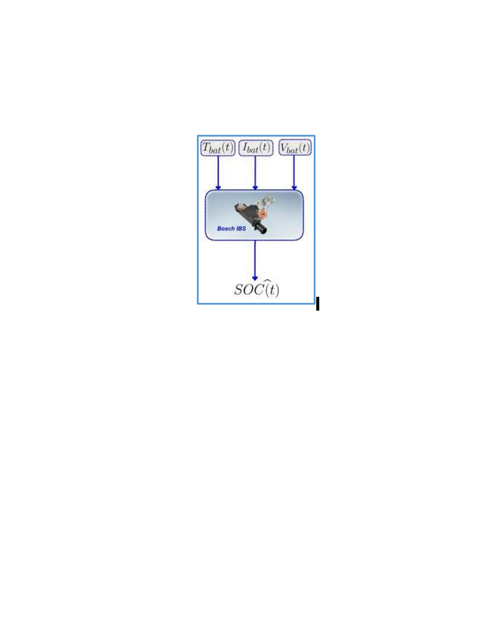
103
Intelligent Battery Sensor (IBS) was installed on the automotive battery. The IBS
software consists of a Kalman filter with a 3rd-order equivalent circuit lead-acid battery
model, and allows for estimation of the battery state of charge with a resolution of 1%.
Figure 54 illustrates the structure of the IBS.
Figure 54: Bosch IBS Kalman Filter Lead-Acid Battery I/O
The battery terminal voltage, current and temperature (𝑉𝑏𝑎𝑡, 𝐼𝑏𝑎𝑡, 𝑇𝑏𝑎𝑡) are the measured
inputs of the Kalman filter, whereas 𝑆𝑂𝐶 (𝑡) is the estimated state variable. The IBS is
directly fastened to the ground terminal of the automotive battery, with a lead wire
coupled to the positive terminal of the battery.
The IBS utilizes a serial network protocol termed LIN (Local Interconnect Network)
which allows for communication between the battery sensor (slave node) and the LIN
controller (master node). LIN is analogous to a single-wire CAN communication
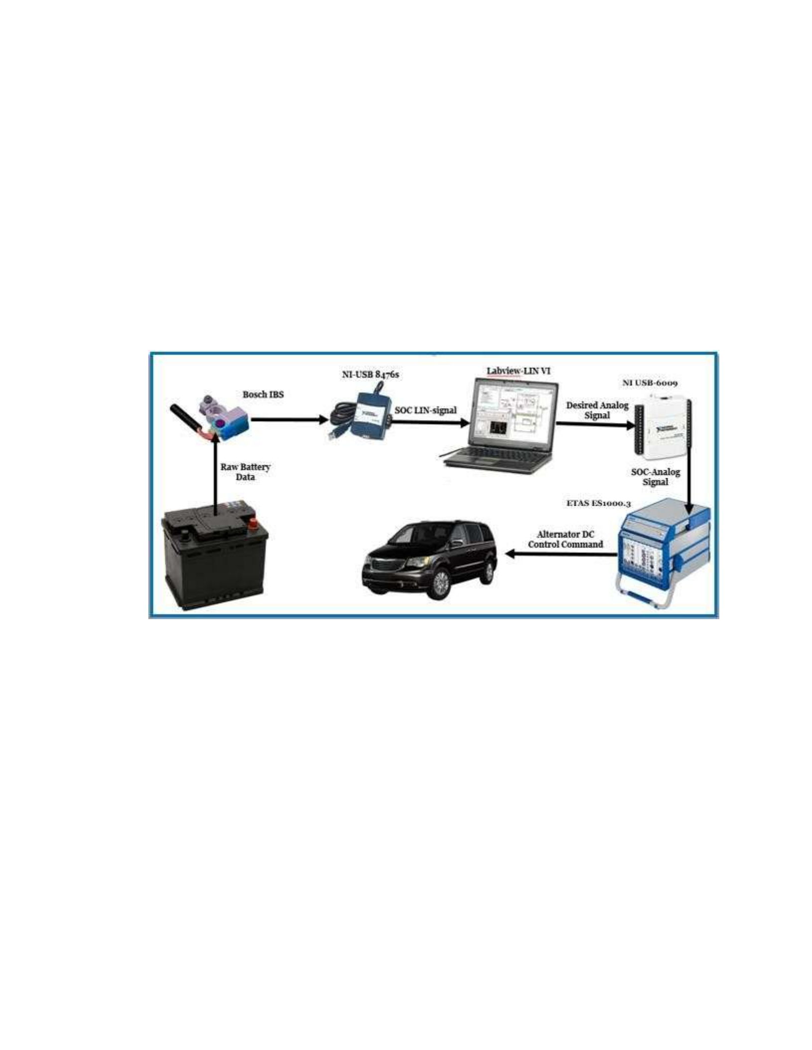
104
network, and sends and receives data frames in hexadecimal format. Thus, there is a need
to translate the LIN hexadecimal data which corresponds to the battery state of charge into
a usable analog voltage signal which may be incorporated into the ETAS system.
Labview 2013, a laptop computer, a National Instruments USB-8476s LIN interface, and a
National Instruments USB-6009 multifunction DAQ are used for this purpose. Figure 55
illustrates the experimental setup used to incorporate the IBS LIN signal into the pre-
existing ETAS system.
Figure 55: IBS Experimental Test Setup
In order to ensure the IBS’ functionality, a validation of the battery sensor is performed.
This task is carried out by comparison of the IBS’ own measured battery current signal
with the battery current signal recorded from the battery shunt. Figure 56 overlays the
battery current, as measured by the battery shunt, with the battery current signal provided
by the Bosch IBS. This data was collected with the vehicle parked and the engine running
under idle conditions. The duty-cycle of the alternator was randomly fluctuated and
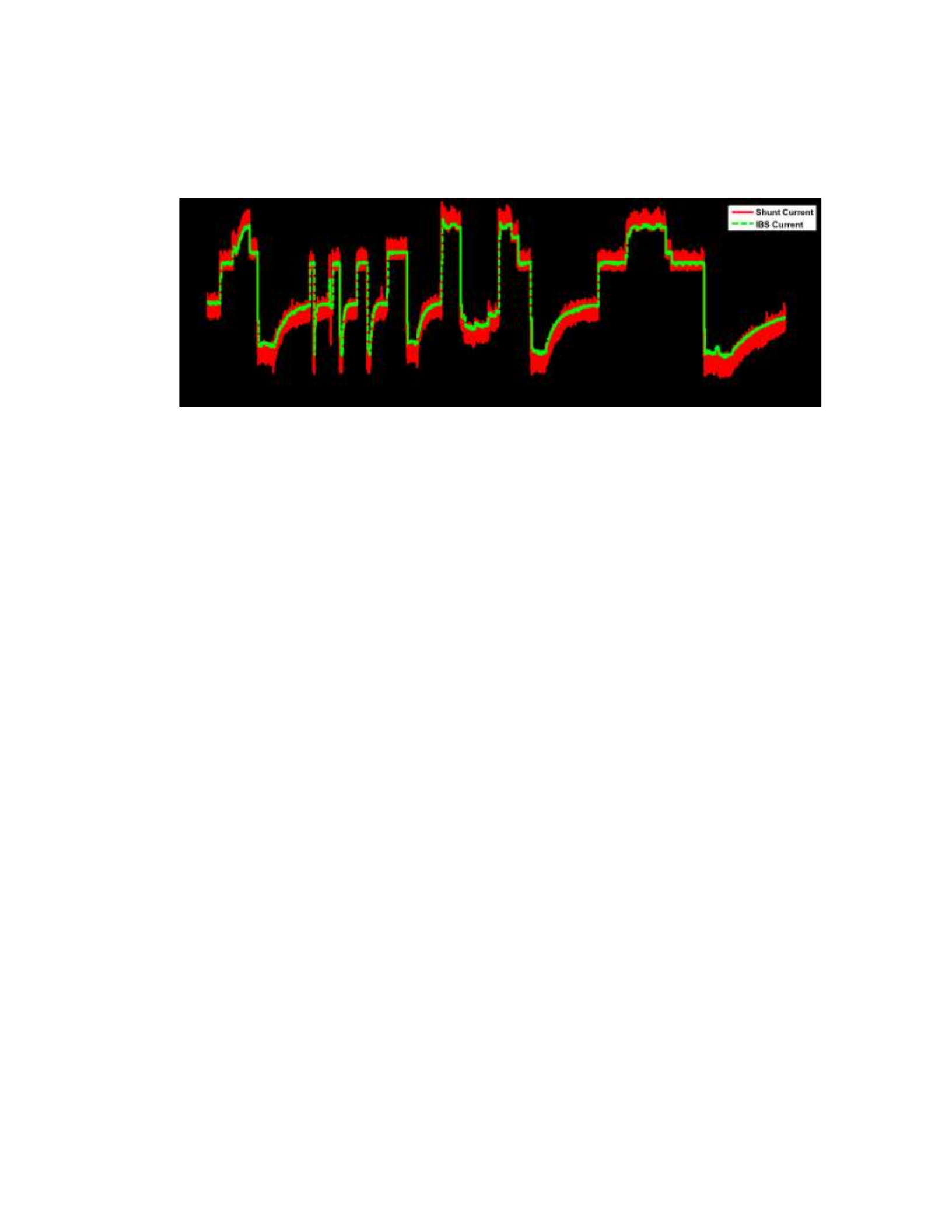
105
various electrical loads were powered on and off, such as the cabin blowers and heated
seats, in order to provide an electrical load profile representative of real-world conditions.
Figure 56: Comparison of Battery Shunt and IBS Battery Current Signal
The IBS battery current signal corresponds with the battery shunt current signal over the
entirety of the electrical load profile considered, which provides an indirect method of
verifying the IBS’ ability to estimate the battery state of charge.
The vehicle, equipped with all necessary testing apparatus, was installed on a light-duty
chassis dynamometer in order to perform numerous regulatory and random “errand” drive
cycles with the A-PMP control strategy activated. More information regarding the
chassis dynamometer experimental setup may be found in Section 2.1.1. Although the
chassis dynamometer does present advantages with respect to determining a given
vehicles fuel economy, certain issues do arise associated with driver inaccuracies and
variations in ambient conditions. In a recent study performed at OSU-CAR, the net fuel
consumption of the vehicle over 8 separate NEDC drive cycles, as calculated by both the
fuel flow-rate signal logged by the ECU and the Big-Grid fuel consumption map, was

106
analyzed. The cycle-to-cycle variation in net fuel consumption was found to exceed 5%
in certain instances. Tables 17 and 18 show the results from this study in cycle-to-cycle
percent variation.
Table 17: Cycle-to-Cycle Percent Fuel Consumption Variation as Calculated by
ECU
NEDC
Cycle No.
1
2
3
4
5
6
7
8
1
-
-0.10
3.02
-1.12
-1.83
-0.32
1.51
1.89
2
0.10
-
3.12
-1.02
-1.74
-0.22
1.61
1.99
3
-3.02
-3.12
-
-4.11
-4.80
-3.33
-1.53
-1.15
4
1.12
1.02
4.11
-
-0.72
0.80
2.62
2.99
5
1.83
1.74
4.80
0.72
-
1.52
3.32
3.69
6
0.32
0.22
3.33
-0.80
-1.52
-
1.83
2.21
7
-1.51
-1.61
1.53
-2.62
-3.32
-1.83
-
0.39
8
-1.89
-1.99
1.15
-2.99
-3.69
-2.21
-0.39
-
Table 18: Cycle-to-Cycle Percent Fuel Consumption Variation as Calculated by
BigGrid Fuel Map
NEDC
Cycle No.
1
2
3
4
5
6
7
8
1
-
-0.26
2.30
-2.57
-3.04
-2.97
-2.16
-2.30
2
0.26
-
2.56
-2.31
-2.78
-2.72
-1.90
-2.04
3
-2.30
-2.56
-
-4.81
-5.27
-5.21
-4.41
-4.54
4
2.57
2.31
4.81
-
-0.48
-0.41
0.42
0.28
5
3.04
2.78
5.27
0.48
-
0.06
0.90
0.76
6
2.97
2.72
5.21
0.41
-0.06
-
0.83
0.69
7
2.16
1.90
4.41
-0.42
-0.90
-0.83
-
-0.14
8
2.30
2.04
4.54
-0.28
-0.76
-0.69
0.14
-
Due to the expected improvements in fuel economy of approximately 1-2%, a different
approach is clearly required in order to estimate the fuel economy benefits which the
APMP control strategy presents over the baseline EVR controller. In order to provide a
baseline for comparing the performance of the A-PMP controller (in-vehicle), simulations

107
were conducted using the VES model together with the model of the Chrysler control
strategy. Such models have been described in Chapter 2. Therefore, the issues associated
with drive cycle repeatability may be mitigated by using engine and electrical load
experimental data collected with the A-PMP activated in conjunction with the VESEVR
model. This approach not only ensures that the same velocity profile is followed for both
control strategies, but also eliminates disparities in vehicle and ambient operating
conditions. In order to estimate the fuel consumption of the vehicle with the APMP
controller in place, the A-PMP experimental data sets are used to calculate the alternator
torque. The alternator torque is then summed with the measured engine torque, and
passed through the Big-Grid fuel consumption map alongside the measured engine speed.
Four different experimental data sets in total are used to analyze the fuel economy benefits
of the A-PMP controller with the aforementioned technique; 2 random “errand” drive
cycles and 2 standardized cycles, one consisting of two consecutive FTPs performed back-
to-back and a second comprised of an EPA driving schedule. The random errand drive
cycles were performed on the chassis dynamometer with no particular velocity trace
observed. The objective of these tests is to emulate a variety of real-world driving
conditions by varying both vehicle velocity and electrical load demand. A “double-FTP”,
as well as the EPA cycle, were performed in order to examine the effects which the
electrical load demand has on the realized fuel savings. The EPA drive cycle was
performed with all electrical accessory loads turned off, and the doubleFTP test was
performed with varying electrical loads (i.e. cabin blowers, radio, heated seats powered on
and off). In this section, the variable load FTP drive cycle as well as one of the two

108
random errand drive cycles are considered. The EPA cycle, as well as the second errand
drive cycle, are analyzed in Section 4.3 for reasons discussed therein. Table 29
summarizes the experimental improvement in fuel economy (over the baseline
EVR controller) for the two drive cycles currently of interest.
Table 19: Experimental Improvement in Fuel Economy due to A-PMP
Drive Cycle
% F.E.
Random Cycle #1
1.4
FTP x2 (Variable Loads)
1.3
The experimental fuel economy observed due to the incorporation of the A-PMP control
strategy into the vehicle electrical system provides for an improvement ranging from
1.31.4%, depending primarily on the velocity and electrical load profile imposed on the
vehicle. In particular, driving schedules which include more frequent acceleration and
deceleration events and require more power from the battery and alternator exhibit
significantly greater fuel savings as opposed to driving schedules with excessive idling
and little electrical load demand. Figures 57-60 illustrate the critical vehicle, engine, and
electrical system behavior for Random Cycle #1.
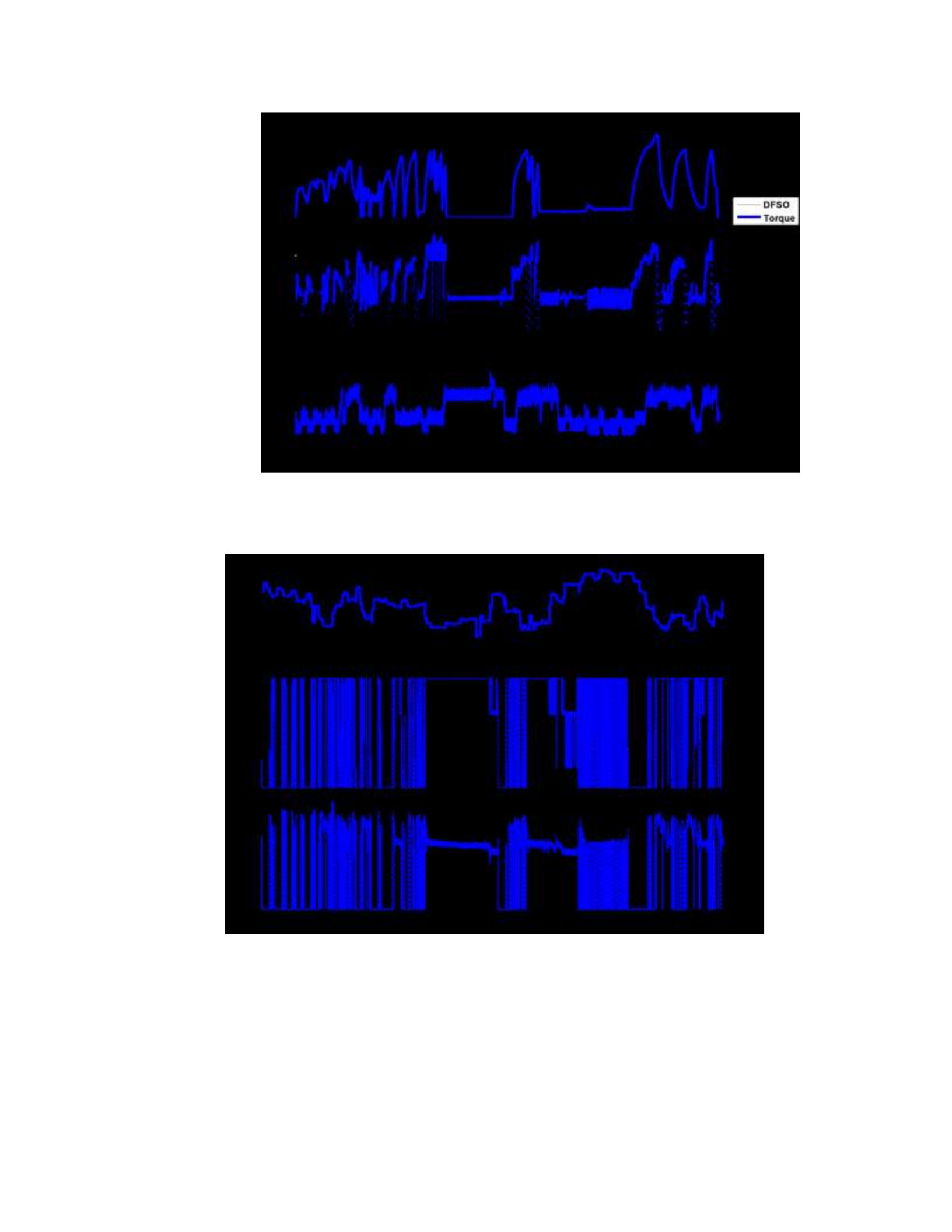
109
Figure 57: A-PMP Experimental Vehicle Behavior, Random Drive Cycle 1
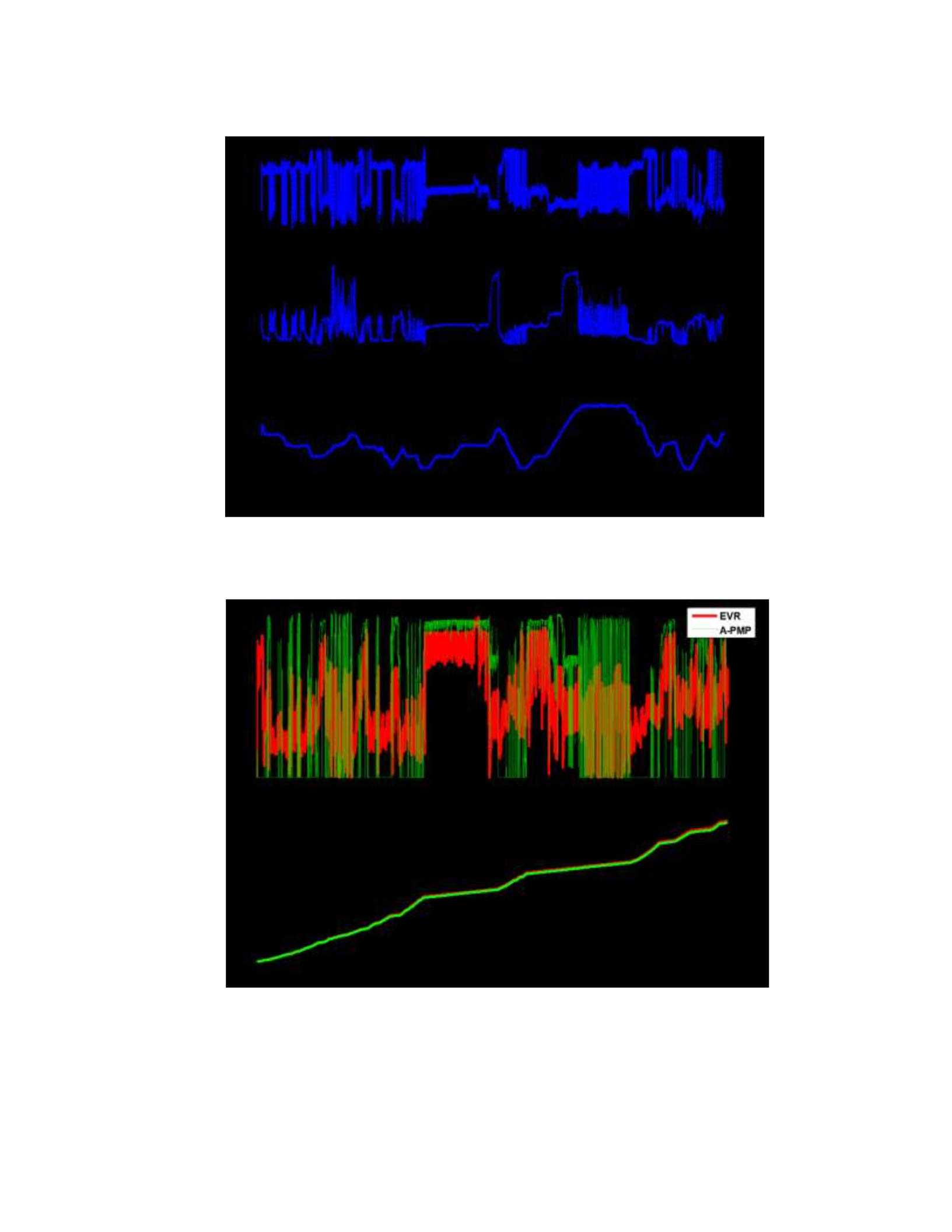
110
Figure 58: A-PMP Experimental Control Behavior, Random Drive Cycle 1
Figure 59: A-PMP Experimental Battery Behavior, Random Drive Cycle 1

111
Figure 60: A-PMP Experimental Fuel Consumption, Random Drive Cycle 1 Of
particular interest is the battery charging/discharging behavior with respect to the
vehicle velocity trace. As discussed in Section 3.2.2, behavior reminiscent of
regenerative braking is observed with the A-PMP controller in place, as may be
observed in Figures 57-60. Hard acceleration events are accompanied by battery
discharge, and coasting/braking leads to battery charging. This behavior agrees very
well with both optimal control and the adaptive control (in simulation), yielding
confidence in the implementation of the controller. Referring to Figure 59, the
battery voltage exceeds 15V (the maximum allowable battery voltage) due to
inaccuracies associated with the 0thorder battery model and the update time of the A-
PMP control strategy (1 second). The battery SOC, on the other hand, remains
confined between 82% and 88%, with highfrequency battery current oscillations
occurring at the upper and lower thresholds due to the activation of the boundary
penalty function, μ. Lambda is observed to reach a maximum value of approximately
-40 as the battery state of charge approaches 88%, illustrating the impact of the state
of charge gain on lambda. Figure 60 compares the
EVR and A-PMP alternator torque profiles along with each control strategies cumulative
fuel consumption. The alternator torque profiles clearly demonstrate the rapid-switching
behavior characteristic of PMP control. The A-PMP alternator torque exceeds that of the
EVR torque under certain circumstances (i.e. vehicle deceleration/coasting), however the
fuel losses incurred at this time are more than replenished (as compared to the EVR) as the
vehicle accelerates and the battery supplies all necessary power to the electrical loads.

112
The EVR leads to a net fuel consumption of 2028g, whereas the vehicle consumes 2000g
of fuel with the A-PMP activated. Figures 61-64 show similar plots for the variable-load
dual-FTP drive cycle. An in-depth discussion regarding the trends observed in the
following figures will be left to the reader, as observations similar to those just noted may
be made.
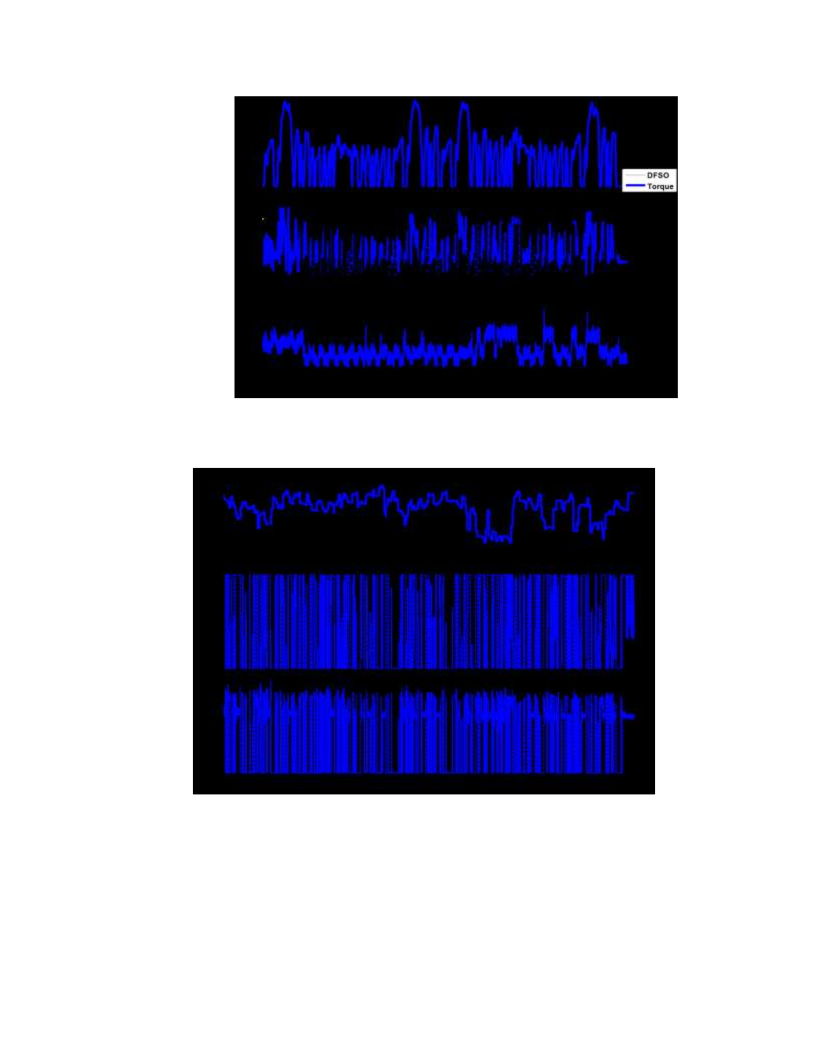
113
Figure 61: A-PMP Experimental Vehicle Behavior, Dual-FTP w/ Variable Loads
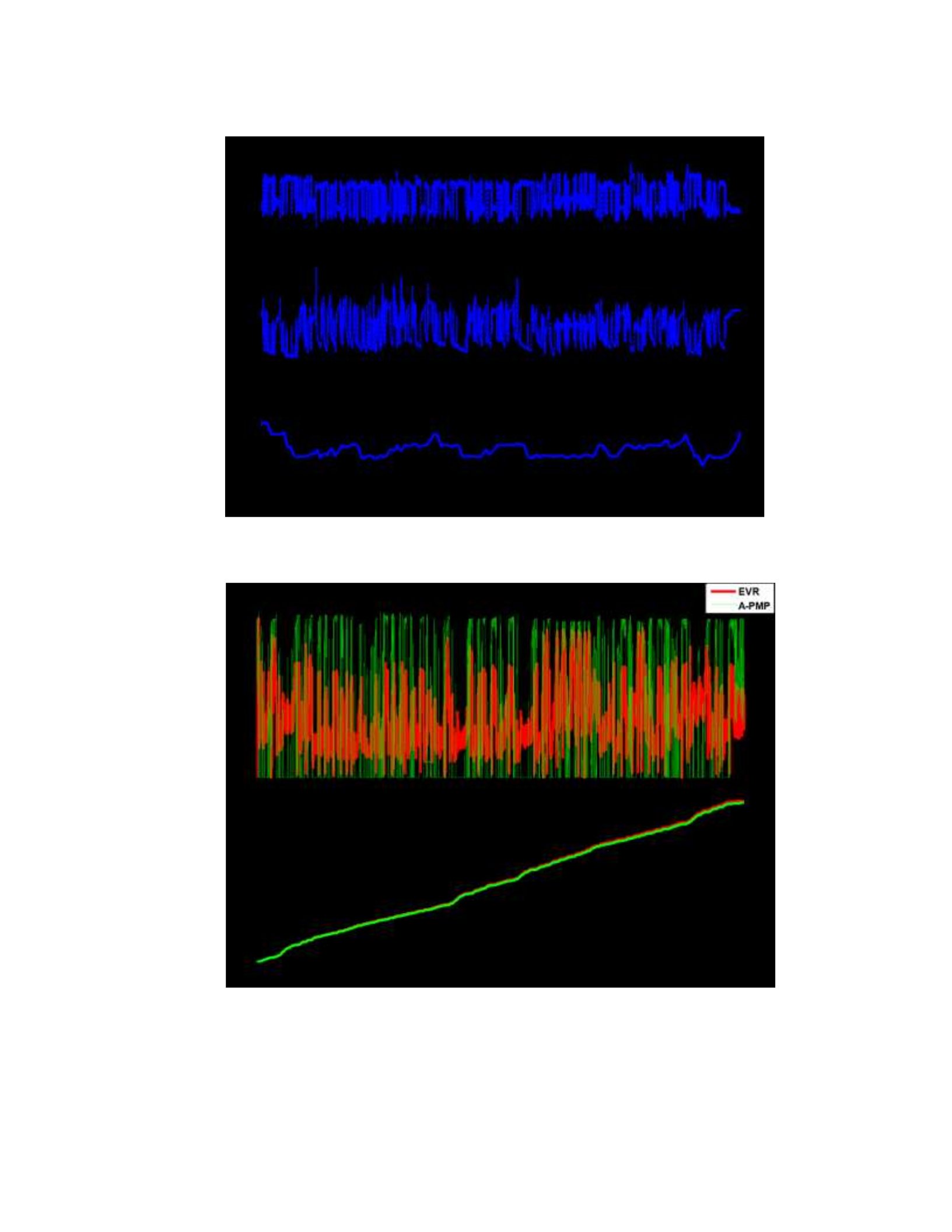
114
Figure 62: A-PMP Experimental Control Behavior, Dual-FTP w/ Variable Loads
Figure 63: A-PMP Experimental Battery Behavior, Dual-FTP w/ Variable Loads

115
Figure 64: A-PMP Experimental Fuel Consumption, Dual-FTP w/ Variable Loads
While consistently beneficial to overall vehicle fuel economy, the A-PMP control strategy
does present issues. The rapid switching behavior observed raises concern regarding
accelerated wear-and-tear of the alternator and driver comfort/safety, and therefore
measures should be taken to mitigate any unnecessary duty-cycle fluctuations.
The battery voltage exceeds the maximum allowable value of 15 V on several occasions.
Finally, although the SOC boundaries are successfully enforced in all experimental drive
cycles, precautions should be taken as to ensure that the battery is never excessively
charged or discharged. For example, if sensors fail and signals become erroneous,
activation of the boundary penalty function may become insufficient to restrict the battery
SOC operating range. Section 4.3 discusses potential solutions to these drivability issues,
and experimentally demonstrates the effects which these solutions have on vehicle
behavior.
Section 4.3: A-PMP Drivability Issues and Solutions
In order to ensure driver safety and comfort and guarantee acceptable VES performance,
three critical issues associated with the A-PMP controller must be addressed:
1. A controller override, which functions as a safeguard against excessive battery
charging/discharging, must be developed and integrated into the A-PMP control
strategy.
2. Modifications to the controller must be made such that troublesome rapid
switching behavior, characteristic of PMP control strategies, is mitigated.

116
3. The controller must be able to eliminate battery voltage spikes exceeding 15V.
Solutions to all 3 issues are developed, integrated into the A-PMP control strategy
discussed in Section 4.1, and tested in-vehicle on the chassis dynamometer. Two
separate experiments are performed on the chassis dynamometer in order to
demonstrate the efficacy of the control modifications; a random “errand” drive
cycle following no particular velocity trace, and an EPA drive cycle with only
baseline electrical loads imposed on the system. It is important to note that for the
two experiments performed in Section 4.3, the allowable battery state of charge
range has been expanded from 82-88% to 80-90%.
4.3.1: Battery State of Charge Controller Override
Battery discharging and charging beyond the imposed state of charge limitations may
result in a variety of undesirable vehicle behaviors, ranging from engine stalling to battery
failure and even no-start conditions. There is thus a need to integrate a battery state of
charge “fail-safe” control strategy into the existing A-PMP control strategy. This control
strategy does not depend on the Hamiltonian to enact the appropriate control command (as
is the case with the boundary penalty function), and is therefore a more reliable method of
ensuring that the battery SOC remains within the allowable operating range. Assuming
that the IBS does not fail, a simple method to implement this control strategy is placing a
logic-based controller on the output of the A-PMP. The “SOCOverride” controller
monitors the battery state of charge, and when an out-of-range SOC value is detected, an
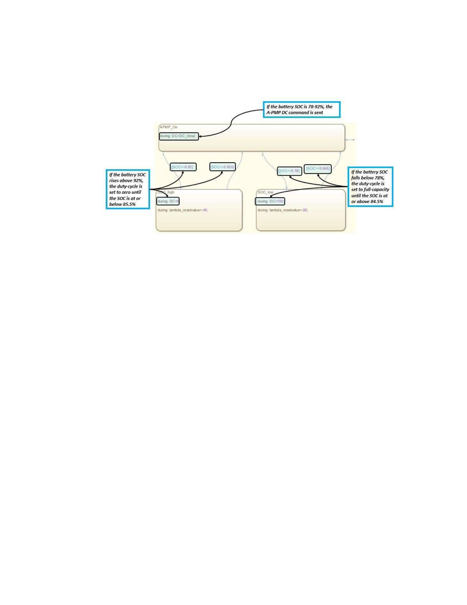
117
override on the duty-cycle command is enacted. This control override is developed in
Mathworks Stateflow, and may be observed in Figure 65.
Figure 65: SOC Override Control Logic Implemented in Stateflow
4.3.2: Bang-Bang Behavior Mitigation and Elimination of Voltage Spikes
The rapid on-off switching behavior, or “Bang-Bang” behavior, which is observed in the
duty-cycle plots featured in Section 4.2.2, will lead to accelerated aging of the alternator,
the auxiliary belt, and possibly other ancillary loads if left untreated. Furthermore, the
oscillations of the alternator duty-cycle lead to excessive charging current during
deceleration events; the root cause of the undesirable battery voltage spikes. This
bangbang behavior is particularly troublesome at low electrical loads (i.e. baseline loads)
during deceleration, and the frequency of oscillations can approach values of
approximately 0.5 Hz. Figure 66 illustrates the severity of this issue over the first 500
seconds of Random Errand Cycle #1. Take note of the consistency with which bangbang
behavior accompanies deceleration events at low load demand.
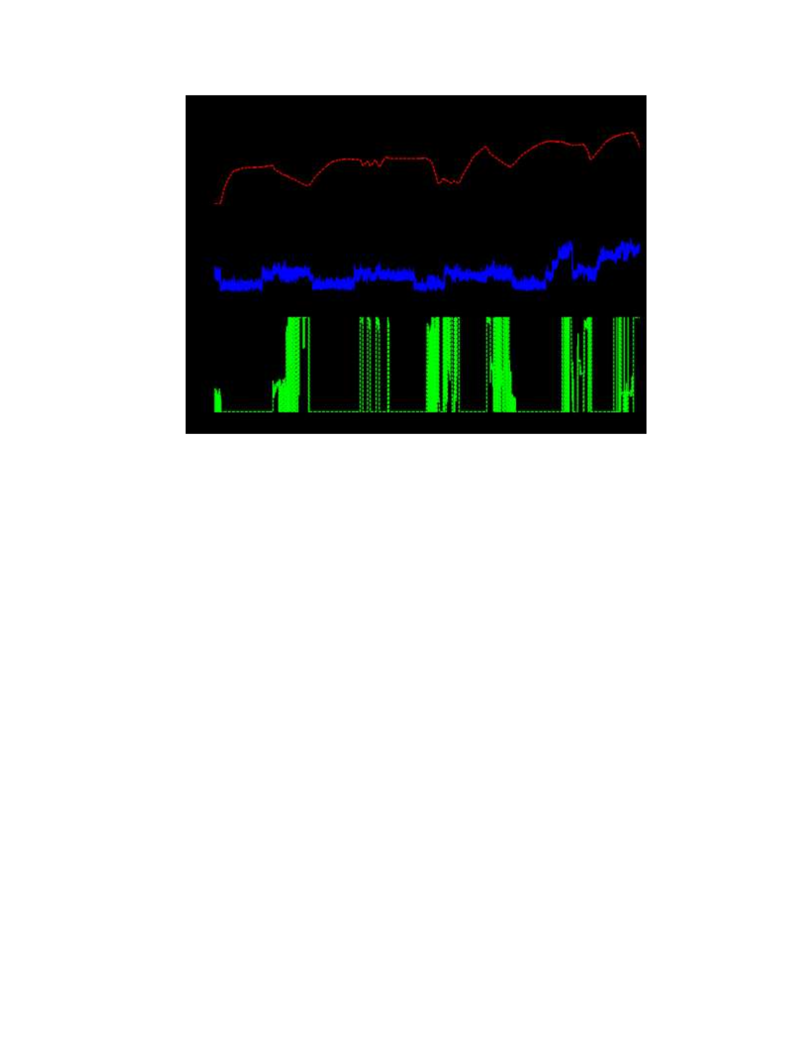
118
Figure 66: Bang-Bang Behavior, Random Drive Cycle #1
The source of the bang-bang behavior may be traced back to the Hamiltonian subsystem,
where the fuel mass flow rate is weighted against the dynamics of the battery state of
charge. As the vehicle accelerator pedal is released at low electrical loads, both the fuel
mass flow rate and battery state of charge dynamics approach minimal values, resulting in
an operating region of instability. The index corresponding to the minimum
Hamiltonian value rapidly oscillates from one extreme (100% duty-cycle) to the other (0%
duty-cycle), thus instigating the undesirable on-off behavior. One possible solution to this
issue may be realized by implementing a filter on the outgoing duty-cycle command. This
mitigates high-frequency duty-cycle dynamics, however numerous unsuccessful in-vehicle
tests at OSU-CAR have demonstrated that this strategy can lead to unacceptably high

119
battery voltages during acceleration due to the lag associated with the duty-cycle
switching from 100% to 0%. Based on the specificity of the problematic vehicle
operating points, a “patch” may be imposed on lambda during deceleration events at low
electrical load demand which forces a predetermined duty-cycle command. As battery
charging is consistently observed during vehicle deceleration, decreasing the costate
variable to a sufficiently negative value provides the desired behavior. The “lambda
patch” monitors both a filtered engine torque signal and the filtered electrical load signal,
activating only when both signals drop below a predetermined value (i.e. the “activation
value”). Table 20 contains the critical lambda patch parameters and values.
Table 20: Lambda Patch Parameter Values
Lambda Override Value
-140
Activation Torque (Nm)
35
Activation Electrical Load (A)
55
The lambda patch parameter values were selected and tuned in-vehicle to ensure that
lambda is only overridden when absolutely necessary in order to mitigate voltage spikes
and bang-bang behavior. Section 4.3.3 features results of two experimental datasets with
the modified A-PMP activated in the minivan.
4.3.3: Modified Controller Experimental Results
The A-PMP controller, complete with the modifications discussed in Sections 4.3.1 and
4.3.2, is implemented in the vehicle and two tests are conducted on the chassis
dynamometer. The first test is an EPA (city plus highway) drive cycle, demonstrating the
co-state override’s ability to mitigate undesirable bang-bang behavior. A random

120
“errand” drive cycle is completed as well, ensuring the modified A-PMP controller’s
performance over a variety of vehicle operating conditions. Table 21 summarizes the
experimental improvement in fuel economy (over the baseline EVR controller) for the two
drive cycles of interest.
Table 21: Experimental Improvement in Fuel Economy due to Modified A-PMP
Drive Cycle
% F.E.
EPA
1.0
Random Cycle #2
1.4
The modifications to the A-PMP controller do not result in any significant decrease in
vehicle fuel economy. Figures 67-70 illustrate the critical vehicle, engine, and electrical
system behavior for the low loads EPA drive cycle. Take special note of the reduction in
duty-cycle bang-bang behavior (illustrated in greater detail in Figure 71) as well as the
elimination of unacceptable battery voltage spikes. Figure 71 compares a roughly 300
second chunk of the modified A-PMP duty-cycle command to that of the original A-PMP
duty-cycle for clarity.
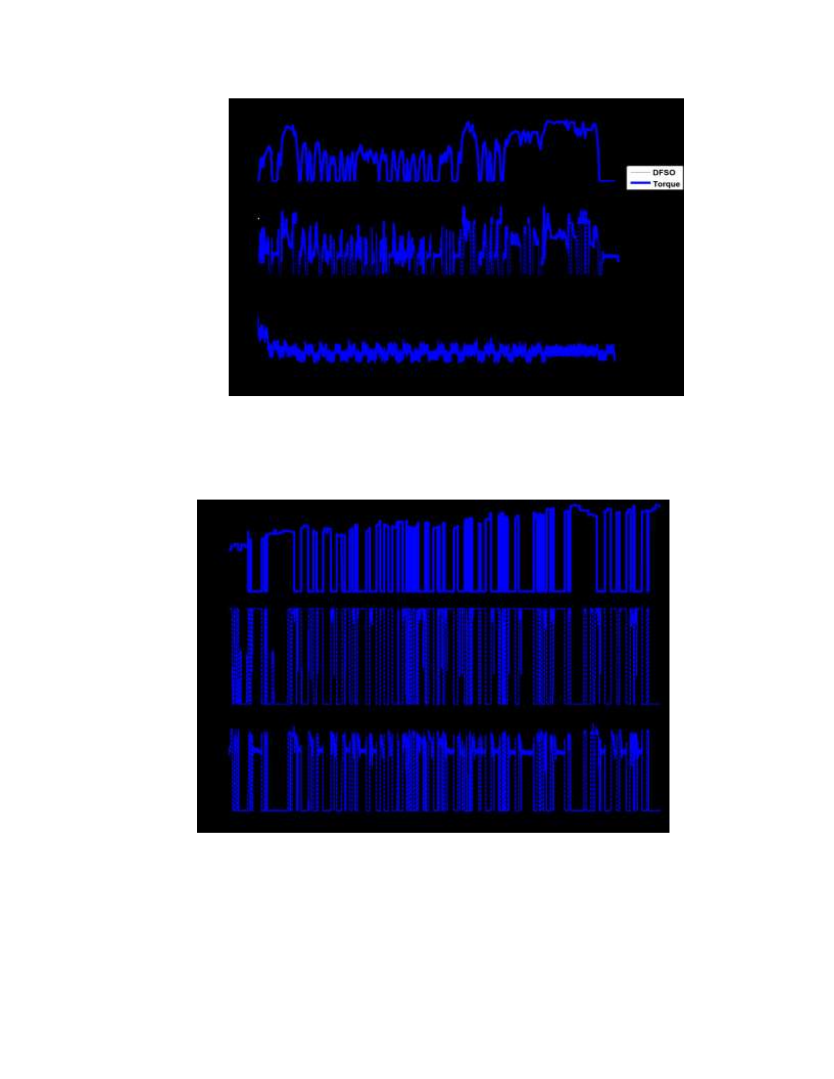
121
Figure 67: Modified A-PMP Experimental Vehicle Behavior, EPA
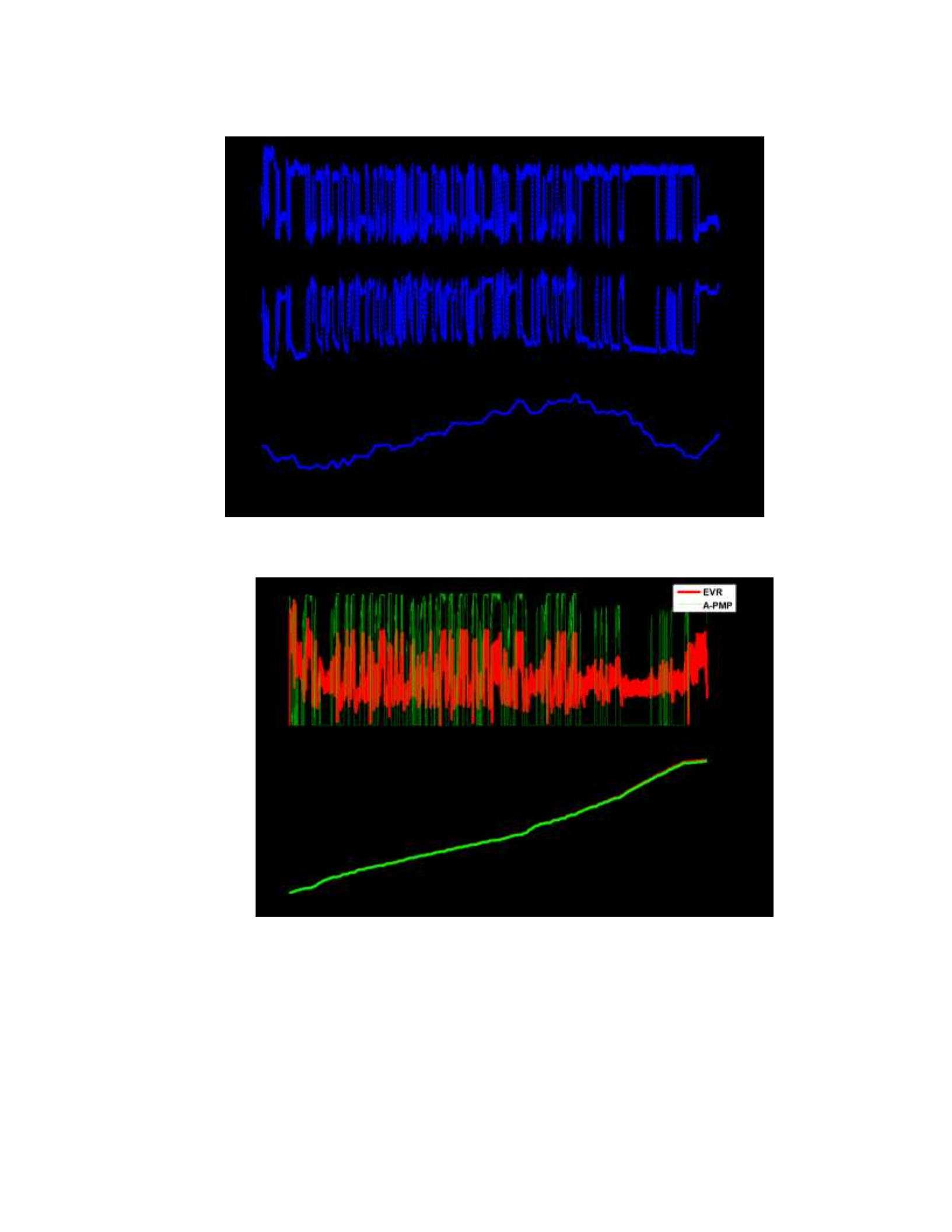
122
Figure 68: Modified A-PMP Experimental Control Behavior, EPA
Figure 69: Modified A-PMP Experimental Battery Behavior, EPA
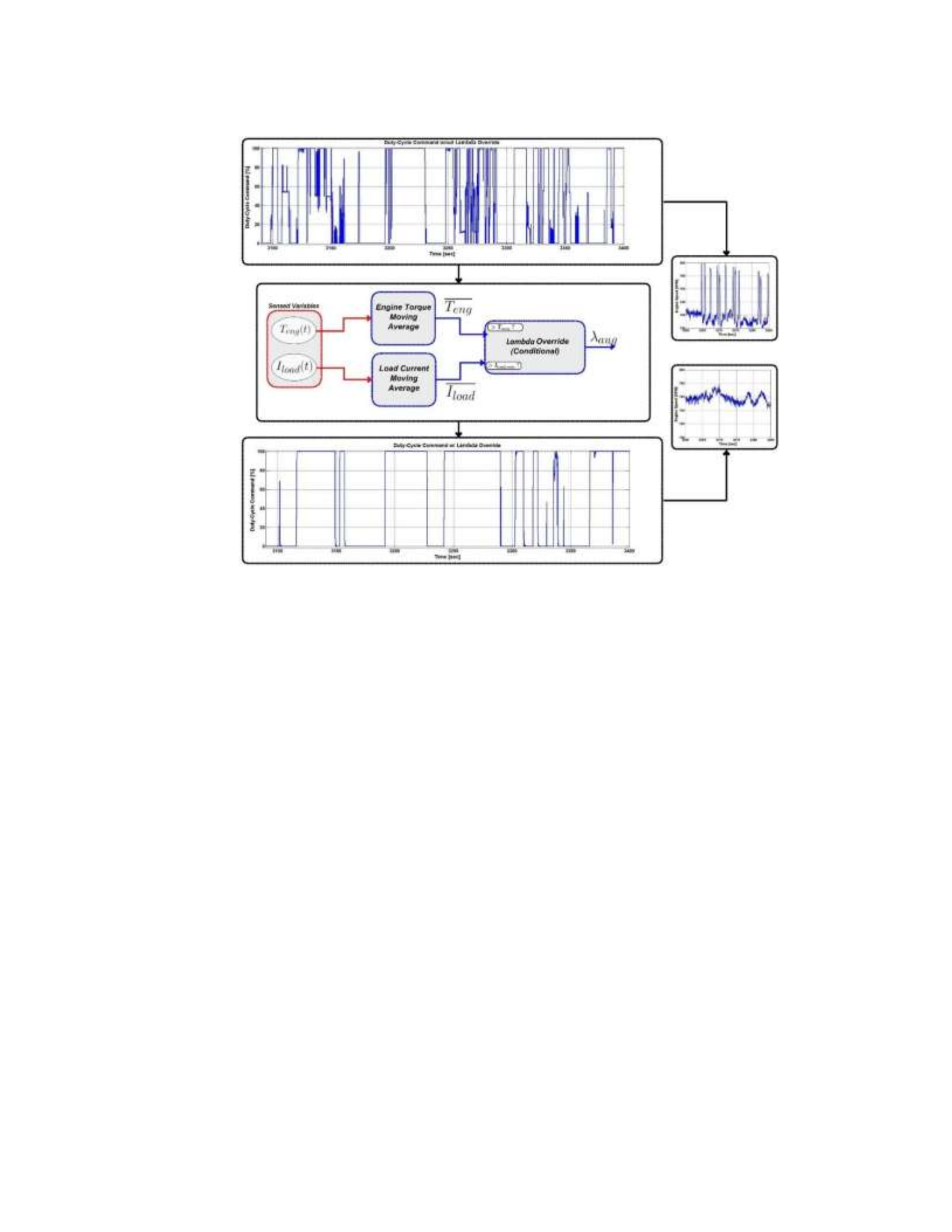
123
Figure 70: Modified A-PMP Experimental Fuel Consumption, EPA
Figure 71: Mitigation of Bang-Bang Behavior
The bang-bang behavior of the A-PMP controller is reduced significantly, as may be
directly observed in Figure 71. Figures 72-75 illustrate the critical vehicle, engine, and
electrical system behavior for Random Drive Cycle #2.
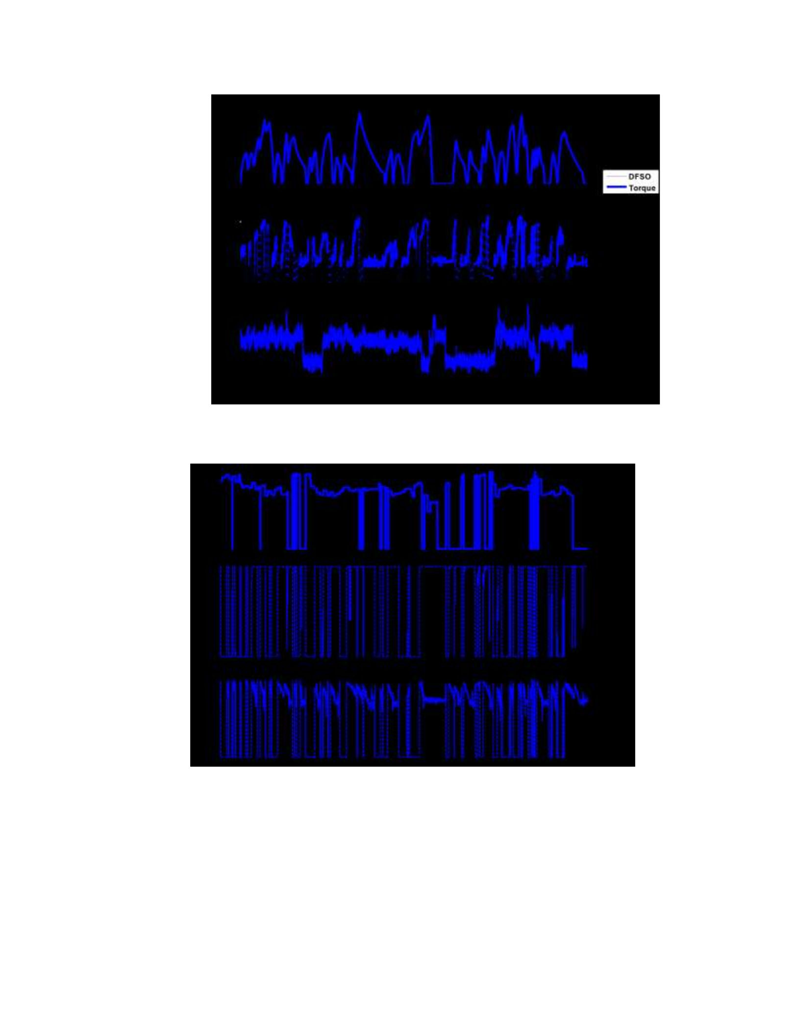
124
Figure 72: Modified A-PMP Experimental Vehicle Behavior, Random Drive Cycle 2
Time [sec]
Figure 73: Modified A-PMP Experimental Control Behavior, Random Drive Cycle
2

125
Figure 74: Modified A-PMP Experimental Battery Behavior, Random Drive Cycle 2
Random "Errand" Drive Cycle #3
Figure 75: Modified A-PMP Experimental Fuel Consumption, Random Drive Cycle
2

126
Adaptations made to the optimal VES control strategy, as described in Chapter 3, have
allowed for the development and implementation of a real-time capable control strategy
which provides significant and consistent experimental improvements in vehicle fuel
economy. Drivability issues relating to both component wear and driver comfort are
addressed, with several possible solutions discussed, implemented and tested online. The
necessary modifications employed have minimal influence on overall vehicle fuel
economy.

127
Chapter 5: Conclusions and Future Work
Section 5.1: Conclusions
The vehicle production alternator control strategy, termed EVR, takes little advantage of
the energy storage capabilities of the onboard automotive battery, simply holding the
battery voltage to some temperature-dependent reference value. While this control
strategy does ensure acceptable cold-cranking performance, significant fuel savings may
be realized by implementing a less conservative VES control which takes advantage of the
battery’s ability to strategically harvest and release energy from the crankshaft. To this
extent, an adaptive controller based on Pontryagin’s Minimum Principle (PMP) is
developed, implemented and tested in-vehicle. This controller is based on critical
observations of VES behavior, in simulation, subjected to optimal control, which requires
all drive cycle information (such as velocity, torque, engine speed, and electrical load
profiles) “a-priori” and is thus impossible to successfully implement in real-time. In order
to facilitate rapid controller development and tuning, virtual prototypes of the vehicle
electrical system, the baseline EVR control strategy, the optimal PMP control strategy, and
the adaptive PMP control strategy are all developed and validated utilizing computerized
behavioral modeling tools. Previous work conducted at OSU-CAR has demonstrated that
the experimental drive cycle to drive cycle variation of the vehicle of interest’s fuel
consumption, as measured by both the ECU and Big-Grid fuel
consumption maps, may exceed 5% in certain instances. Concerns regarding this issue are
mitigated by conducting dynamometer testing with the A-PMP activated, and comparing
the experimental A-PMP fuel economy to the validated EVR model’s fuel economy.

128
Utilizing these analysis techniques, the A-PMP demonstrates consistent experimental
improvements in vehicle fuel economy ranging from 1.1-1.4%. Drivability issues such as
accelerated alternator wear-and-tear and unacceptable battery behavior (i.e. excessive
charging/discharging) are addressed. Solutions to these issues are implemented and tested
in-vehicle, demonstrating negligible effects on overall vehicle fuel economy.
Section 5.2: Future Work
While the present work experimentally demonstrates the potential of an adaptive,
PMPbased control strategy to improve vehicle fuel economy while maintaining driver
comfort and component reliability, numerous opportunities for extending the scope of this
research exist. Completion of the following tasks may allow for further increases in
vehicle fuel economy and more precise estimations of the fuel economy benefit which the
A-PMP control strategy brings about.
1. Improved VES Model. The fully integrated Vehicle Electrical System model,
composed of a battery, alternator, and EVR model, has been validated and agrees
well with experimental data sets collected across a wide variety of operating
conditions. Nonetheless, due to the nature of the analysis techniques used to
estimate the A-PMP fuel economy benefit, a more precise VES model would
provide useful insight into the experimental vehicle fuel consumption of the
EVRequipped vehicle. The development of an alternator model which is not
strictly based on empirically-derived steady-state data and takes into account the
dynamics of the alternator may prove useful to this extent [22].

129
2. Expansion of Optimal Control to Load Shedding. Just as strategic utilization of
the alternator and battery reduces overall vehicle fuel consumption, selective
reduction of the electrical load demand may allow for more fuel-efficient VES
behavior. Studies similar to those performed in Section 3.2, and the resulting
experiments described in Section 4.2, may therefore be expanded to allow for a
temporary reduction in electrical load demand. This would require the
incorporation of a separate term into the Hamiltonian function with an adaptive co-
state variable. Furthermore, experimental calibration of the allowable time for
which a load may be shed would need to be carried out to ensure driver comfort.

130
References
[1] “Number of Drivers and Motor Vehicles in the United States, 1960-2009.” Earth
Policy Institute, 2012.
[2] “US Auto Industry sees best sales since 2007; recovery expected to slow in
2014.” Michigan Local News, 2013.
[3] “The Road to 2020 and Beyond: What’s Driving the Global Automotive
Industry?” Advanced Industries, 2013.
[4] “Highway Statistics 2007; Licensed Drivers, Vehicle Registrations, and Resident
Population.” U.S. Department of Transportation, Federal Highway Administration,
2012.
[5] “Annual Energy Outlook 2013.” U.S. Energy Information Administration, 2013.
[6] F. Chiara, M. Canova, and G. Rizzoni. “Future Mobility Challenges, Where Will
We Find Fuel Efficient Solutions?” The Ohio State University, 24 April 2012.
Print.
[7] “Frost and Sullivan Analysis Suggests Momentum toward Supplementary 48V
On-board Power-net.” Green Car Congress, 2012.
[8] “Automakers Expanding 48-V Production Plans, says AVL Electrification Chief.”
SAE International, 2014.
[9] Chong, Andrew. “Driving Asia – As Automotive Electronics Transforms a
Region.” Infineon Technologies Asia Pacific Pte Ltd, 2010. Print.
[10] Hardin, Christopher. “Effect of Automotive Electrical System Changes on Fuel
Consumption Using an Incremental Efficiency Methodology.” Thesis.
Massachusetts Institute of Technology, 2004. Print.
[11] Bryson, Arthur. “Optimal Control – 1950-1985.” IEEE Control Systems, 1996.
[12] N. Kim, C. Sukwon, H. Peng. “Optimal Control of Hybrid Electric Vehicles
Based on Pontryagin’s Minimum Principle.” IEEE Transactions on Control
Systems, 2011.

131
[13] D. Ambuhl, O. Sundstrom, A. Sciarretta, L. Guzzella. “Explicit Optimal Control
Policy and its Practical Application for Hybrid Electric Powertrains.” IFAC
Journal Of Control Engineering Practice, 2010.
[14] X. Zhang, C. Mi. “Vehicle Power Management: Modeling, Control and
Optimization.” Springer, 2011. Print.
[15] J. Liu, H. Peng. “Modeling and Control of a Power-Split Hybrid Vehicle.” IEEE
Transactions on Control Systems Technology, 2008.
[16] S. Onori and L. Serrao. “On Adaptive-ECMS Strategies for Hybrid Electric
Vehicles.” Les Rencontres Scientifiques d’IFP Energies Nouvelles, 2011. Print.
[17] S. Onori, L. Serrao, G. Rizzoni. “Adaptive Equivalent Consumption
Minimization Strategy for Hybrid Electric Vehicles.” Proceedings of the ASME
2010 Dynamic Systems and Control Conference, 2010.
[18] S. Stockar, V. Marano, M. Canova, G. Rizzoni, L. Guzzella. “Energy-Optimal
Control of Plug-in Hybrid Electric Vehicles for Real-World Driving Cycles.”
IEEE Transactions on Vehicular Technology, 2011.
[19] J. Kessels, M. Koot, B. Jager, P. Bosch, N. Aneke, D. Kok. “Energy
Management for the Electric Powernet in Vehicles with a Conventional
Drivetrain.” IEEE Transactions on Control Systems Technology, 2007.
[20] J. Couch, M. Canova, L. Fiorentini. “An ECMS-based Approach for the Energy
Management of a Vehicle Electrical System.” The International Federation of
Automatic Control, 2013.
[21] Ma, Xiaoliang. “Optimal Controls of Fleet Trajectories for Fuel and Emissions.”
IEEE Intelligent Vehicles Symposium, 2013.
[22] A. Scacchioli, G. Rizzoni, M. Salman, W. Li, S. Onori, X. Zhang. “Model-based
Diagnosis of an Automotive Electric Power Generation and Storage System.”
IEEE Transactions on Systems, Man, and Cybernetics: System, 2014.
[23] Ceraolo, Massimo. “New Dynamic Models of Lead-Acid Batteries.” IEEE
Transactions on Power Systems, 2000.
[24] N. Moubayed, J. Kouta, A. El-Ali, H. Dernayka, R. Outbib. “Parameter
Identification of the Lead-Acid Battery Model.” IEEE Paper 978-1-4244-1641-7.

132
[25] Mayer, D. “Modelling and Analysis of Lead Acid Battery Operation.”
Telecommunications Energy Conference, 1989.
[26] A. Scacchioli, G. Rizzoni, and P. Pisu. “Model-Based Fault Detection and
Isolation in Automotive Electrical Systems.” ASME International Mechanical
Engineering Congress and Exposition, 2006. Print.
[27] Y. Hu, S. Yurkovich, Y. Guezennec, and B.J. Yurkovich. “Electro-Thermal Battery
Model Identification for Automotive Applications.” Journal of Power Sources
196, 2011. Print.
[28] Jackey, Robyn. A. “A Simple, Effective Lead-Acid Battery Modeling Process for
Electrical System Component Selection.” SAE Paper 2007-01-0778.
[29] Jiang, Shugang. “A Parameter Identification Method for a Battery Equivalent
Circuit Model.” SAE Paper 2011-01-1367.
[30] K. Salloux, J. McHardy. “Eliminating Battery Failure – Two New Leading
Indicators of Batterry Health – A Case Study.” IEEE Telecommunications Energy
Conference, 2007.
[31] Couch, Jeremy. “An ECMS-based Controller for the Electrical System of a
Passenger Vehicle.” Thesis. The Ohio State University, 2013.
[32] S. Chiniforoosh, A. Davoudi, P. Alaeinovin, J. Jatskevich. “Dynamic Modelling
and Characterization of Vehicular Power System Considering Alternator Iron
Core and Rectifier Losses.” IET Electrical Systems in Transportation, 2012.
[33] Yedeg, Esubalewe. “Control and Design of Engineering Mechanics Systems.”
Thesis. Umea University, Sweden, 2013.
[34] L. Serrao, S. Onori, G. Rizzoni. “ECMS as a Realization of Pontryagin’s
Minimum Principle for HEV Control.” American Control Conference, 2009

