


PSYC 355
SPSS HOMEWORK: CORRELATION ASSIGNMENT
Katherine Crisco
School of Behavioral Science, Liberty University
PSYC 355: Statistics in Psychology
Dr. Haynes
SEPTEMBER 22, 2025
Problem Set 1: Pearson Correlation Coefficient Analysis CHANGE NUMBERS
Research Scenario: Fake reviews of online products have been on the rise over the last decade,
where individuals or firms are paid to provide positive or negative reviews of products they have
not actually purchased to sway future consumers. An industrial/ organizational psychologist at a
large online retailer wants to determine whether there is a relationship between fake positive
reviews (which present a product as probably better than it really is) and the number of
customer returns. He records the number of positive reviews from unverified purchasers as well
as the total number of times each product was returned over the course of 6 months. The data
for twelve of these products are entered into the table below.
Using this table, enter the data into a new SPSS data file and run a Pearson correlation
coefficient analysis to test whether there is a relationship between the number of fake
positive reviews for a product and the number of customer returns. Create a scatterplot to
display the relationship between the variables. Remember to put your initials within any and
all variable names. Follow the directions below the table to complete the homework.
Fake Positive
Reviews
Total Number
of Returns

PSYC 355
1. Paste SPSS output. (10 pts) 2.
2. Write an APA-style Results section based on your analysis.
Include your scatterplot as an APA-style Figure, with figure
number and title, as demonstrated in the Results Section
presentation. (Results = 12 pts; Figure = 8 pts)
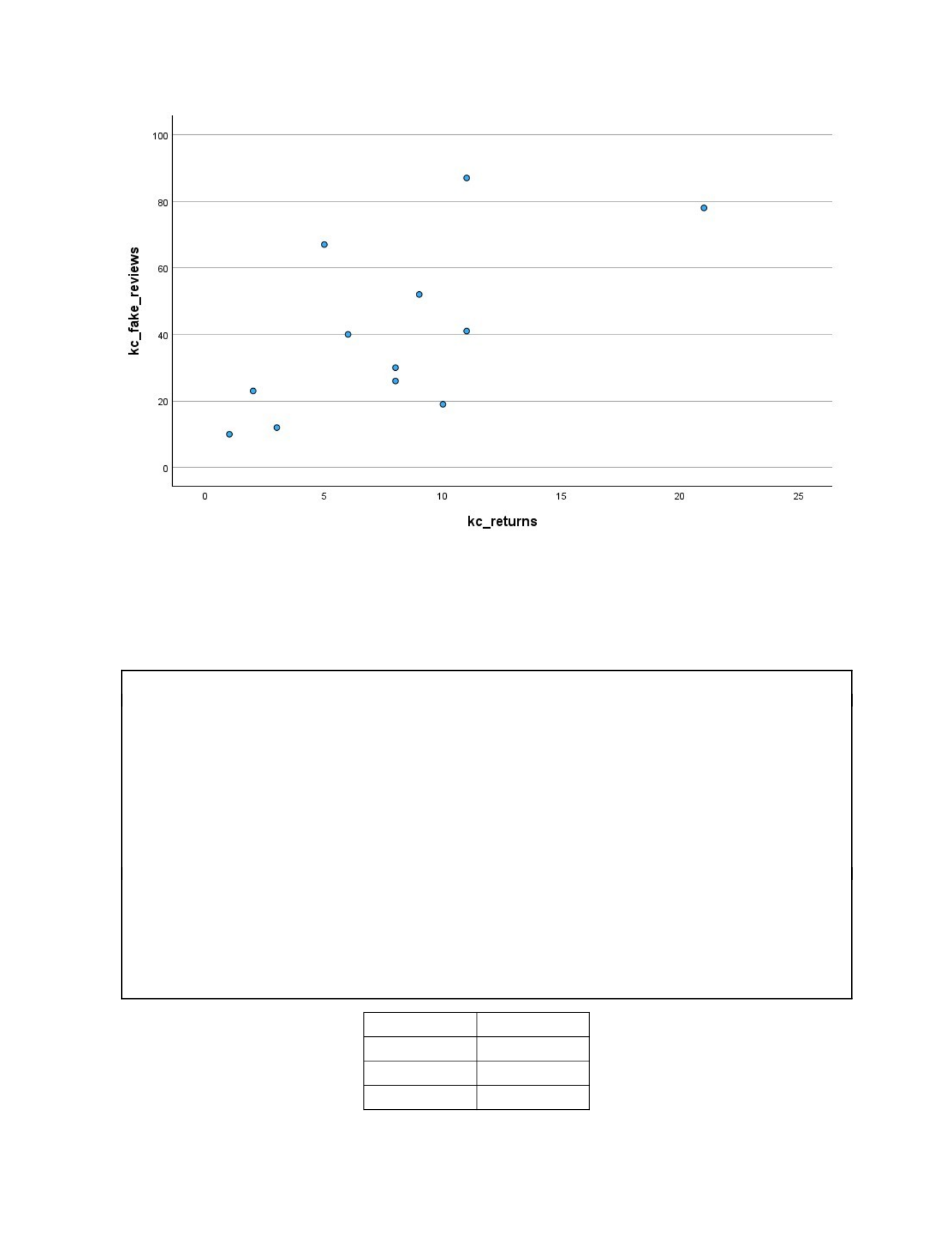
A Pearson correlation coefficient was conducted and computed to see if the relationship
between the fake reviews, which are fake positive reviews, and the overall total number of
returns. The results show a significant positive relationship between the variables, which is
r(10)=0.649, p=0.02. In addition, the fake positive reviews ultimately increase, and the total
number of returns increases slightly. Therefore, it rejected the null hypothesis that shows a
correlation between these variables, which is zero. The figure below shows the relationship
between Fake Positive reviews and the total number of returns
PSYC 355
Problem Set 2: Pearson Correlation Coefficient Analysis
Research Scenario: Recent research into the effects of climate-based events on mental health
suggests that climate anxiety is on the rise, especially among younger people. A clinical
psychologist would like to determine whether there is a relationship between age and climate
anxiety. She administers the Climate Change Anxiety Scale (CCAS; Clayton, S., & Karazsia, B. T.,
2020) to 22 adults between the ages of 18 and 65. Scores on the CCAS range from 22 to 110,
with higher scores indicating higher climate anxiety and cognitive and functional impairment
related to the anxiety. The data are listed in the table below.
Using this table, enter the data into a new SPSS data file and run a Pearson correlation
coefficient analysis to test whether there is a relationship between age and scores on the
CCAS. Create a scatterplot to display the relationship between the variables. Remember to put
your initials within any and all variable names. Follow the directions below the table to
complete the homework.
Age CCAS Score
47 45
52 23
60 30

PSYC 355
61 26
20 66
39 54
39 28
59 40
40 50
26 98
57 33
23 38
60 25
37 29
19 83
27 62
55 31
60 30
32 60
30 73
46 27
24 88
1. Paste SPSS output. (10 pts)
Correlations
kc_age kc_CCAS
kc_age Pearson Correlation 1 -.771**
Sig. (2-tailed) <.001
N22 22
kc_CCA S Pearson Correlation -.771** 1
Sig. (2-tailed) <.001
N22 22
**. Correlation is significant at the 0.01 level (2tailed).
2. Write an APA-style Results section based on your analysis. Include your scatterplot as an
APA-style Figure, with figure number and title, as demonstrated in the Results Section
presentation. (Results = 12 pts; Figure = 8 pts)
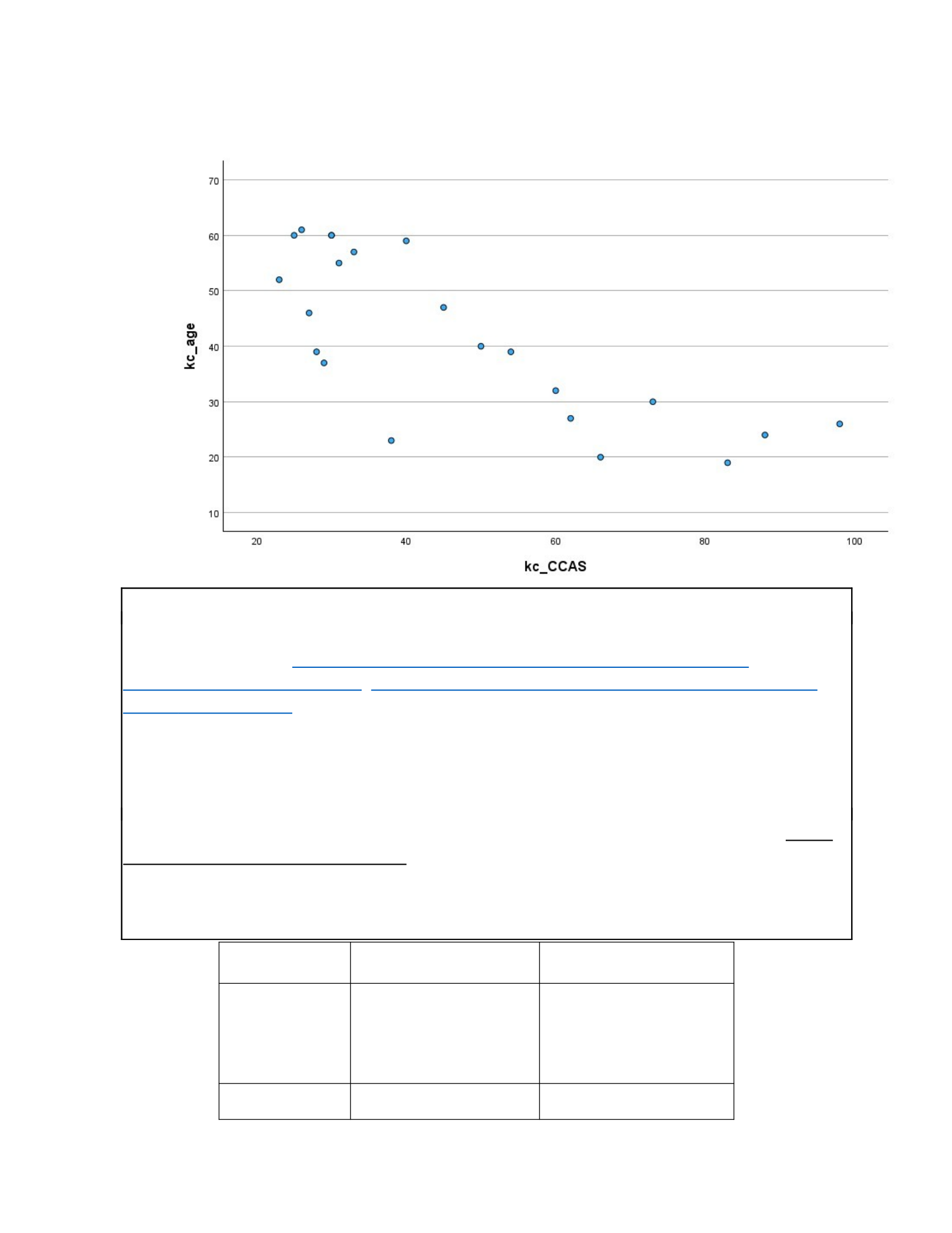
A Pearson correlation coefficient was used to see if the relationship between age and the
climate change anxiety scale, which is CCAS. The overall results show a significant and
negative relationship between the variables, which is r(20)=-.771, p=0.001. In addition,
the age decreases the CCAS scores decrease. Therefore, it rejected the null hypothesis
PSYC 355
and that the relationship and correlation between these variables is zero. The graph
below shows the relationship between age and the climate change anxiety scale.
Problem Set 3: Cumulative Knowledge Question
Research Scenario: In response to recent Gallup and Pew Center polls of Americans’ trust in
their political leaders (https://news.gallup.com/poll/512651/americans-trust-local-
government congress-least.aspx ; https://www.pewresearch.org/politics/2022/06/06/public-
trust-in government-2/ ), a social psychologist decides to study people’s trust in politicians among
different political parties and regions in his state. The psychologist administers a scale-level
questionnaire with possible scores ranging from 1-30, with higher scores indicating higher trust
in politicians, and lower scores indicating lower trust. The data from this scale-level
questionnaire are shown in the table below.
Using this table, enter the data into a new SPSS data file. Choose the correct analysis (it will
be one learned in a previous module) to determine whether there is a difference in trust
scores depending on political party and region. Choose and create the correct graph that
corresponds with this analysis. Remember to put your initials within any and all variable
names. Follow the directions below the table to complete this part.
1.Urban 2.Rural
1.Republican 16
15
29
18
19
28
29
30
2.Democrat 30 19

PSYC 355
24
28
15
14
16
20
3.Libertarian 21
12
10
9
9
18
15
11
4.Independen
t
15
23
6
21
15
9
15
13
1. Paste SPSS output. (10 pts)
Descriptive Statistics
Dependent Variable: score_kc
Std.
Area_kc Party_kc Mean Deviation N
Urban Republican19.50 6.455 4 Democrat 24.25 6.652 4
Libertarian 13.00 5.477 4
Independen
t
16.25 7.632 4
Total 18.25 7.298 16
Rural Republican 26.50 5.066 4
Democrat 17.25 2.754 4
Libertarian 13.25 4.031 4
Independen
t
13.00 2.828 4
Total 17.50 6.583 16
Total Republican 23.00 6.547 8
Democrat 20.75 6.018 8
Libertarian 13.13 4.454 8
Independen
t
14.63 5.605 8
Total 17.88 6.847 32
Between-Subjects Factors
Value Label N

PSYC 355
Area_kc 1 Urban 16
2 Rural 16
Party_kc 1 Republican 8
2 Democrat 8
3 Libertarian 8
4 Independent 8
Tests of Between-Subjects Effects
Dependent Variable: score_kc
Source
Type III Sum of
Squares df Mean Square F Sig.
Partial Eta
Squared
Corrected Model 758.500a7 108.357 3.742 .007 .522
Intercept 10224.500 1 10224.500 353.076 <.001 .936
Area_kc 4.500 1 4.500 .155 .697 .006
Party_kc 541.250 3 180.417 6.230 .003 .438
Area_kc * Party_kc 212.750 3 70.917 2.449 .088 .234
Error 695.000 24 28.958
Total 11678.000 32
Corrected Total 1453.500 31
a. R Squared = .522 (Adjusted R Squared = .382)
Multiple Comparisons
Dependent Variable: score_kc
Tukey HSD
(I) Party_kc (J) Party_kc
Mean Difference
(I-J) Std. Error Sig.
95% Confidence Interval
Lower Bound Upper Bound
Republican Democrat 2.25 2.691 .837 -5.17 9.67
Libertarian 9.88*2.691 .006 2.45 17.30

PSYC 355
Independent 8.38*2.691 .023 .95 15.80
Democrat Republican -2.25 2.691 .837 -9.67 5.17
Libertarian 7.62*2.691 .043 .20 15.05
Independent 6.12 2.691 .132 -1.30 13.55
Libertarian Republican -9.88*2.691 .006 -17.30 -2.45
Democrat -7.62*2.691 .043 -15.05 -.20
Independent -1.50 2.691 .944 -8.92 5.92
Independent Republican -8.38*2.691 .023 -15.80 -.95
Democrat -6.12 2.691 .132 -13.55 1.30
Libertarian 1.50 2.691 .944 -5.92 8.92
Based on observed means.
The error term is Mean Square(Error) = 28.958.
*. The mean difference is significant at the .05 level.
2. Write an APA-style Results section based on your analysis. Include your graph as an APA-
style Figure, with figure number and title, as demonstrated in the Results Section
presentation. (Results = 12 pts; Figure = 8 pts)
A two-way ANOVA test was done to see if there is any difference in the State regions, which is
rural and urban, and the political party, which was Republican, Democrat, Libertarian, and
Independent, on a scale level questionnaire scores. The scores indicate the amount of trust
individuals have in politicians. In addition, the graph below shows the trust scores in the state
regions and the political parties. The overall main effect of political parties was found to be
significant, F(3,24)=6.23, p = 0.003, and the partial eta squared = 0.438. Post Hoc test, which
used Turkey s HSD test, showed that the Libel Party's M=13.13, SD=4.454, and the Independent
Party's M=14.63, SD=5.605 had significantly lower the politicians' trust scores than the
Republican Party's M=23, SD=6.547 or the Democratic Party's M=20.75, SD=6.018, p=0.006
regardless of the state regions. Therefore, it rejected the null hypothesis that there is no effect
of political party on the trust scores. In addition, the main effect of the state region was found
to be significant F(1,24) =0.155, p=0.697, and the partial eta squared=0.06. Therefore, it failed
to reject the null hypothesis of the state region on the political trust scores. In the end, the
interaction of the political parties and the state area was not significant F(3,24)=2.449, p=0.088,

PSYC 355
and the partial eta squared = 0.234. After all, it was significant to reject the null hypothesis that
the effect of political parties on the trust scores is about the same across both state areas.

