


Running head: ANCOVA
GROUP #3 WRITE-UP: ANCOVA
Partial Fulfillment
Of the Requirements for EDUC 812
Liberty University
2019
1

ANCOVA 2
FINDINGS
Research Question
The research question for this study was:
RQ: Is there a significant difference between the depression scores of students who
receive Journal and Counseling therapy, Journal therapy only, or Counseling therapy only, when
controlling for pre-test depression scores?
Null Hypothesis
The null hypothesis for this study was:
H0: There is no significant difference among the depression scores of students who
receive Journal and Counseling therapy, Journal therapy only, or Counseling therapy only, while
controlling for pre-test depression scores.
Descriptive Statistics
Data obtained for the dependent variable depression score was obtained for each of the
three therapy groups: Journal and Counseling (JC), Counseling Only (C ), and Journal Only (J).
Means and standard deviations were calculated both pre-treatment and post-treatment (see Table
1).
Table 1
Descriptive Statistics
Measure Group M SD N Adjusted SE
Mean
Pre-Test JC 69.30 11.58 20
J 65.65 10.02 20
C 70.95 10.51 20
Post-Test JC 70.30 7.98 20

ANCOVA 3
J 65.85 8.38 20
C 71.10 7.21 20
Estimates JC 20 69.94 1.22
J 20 67.44 1.24
C 20 69.86 1.23
Results
Data screening
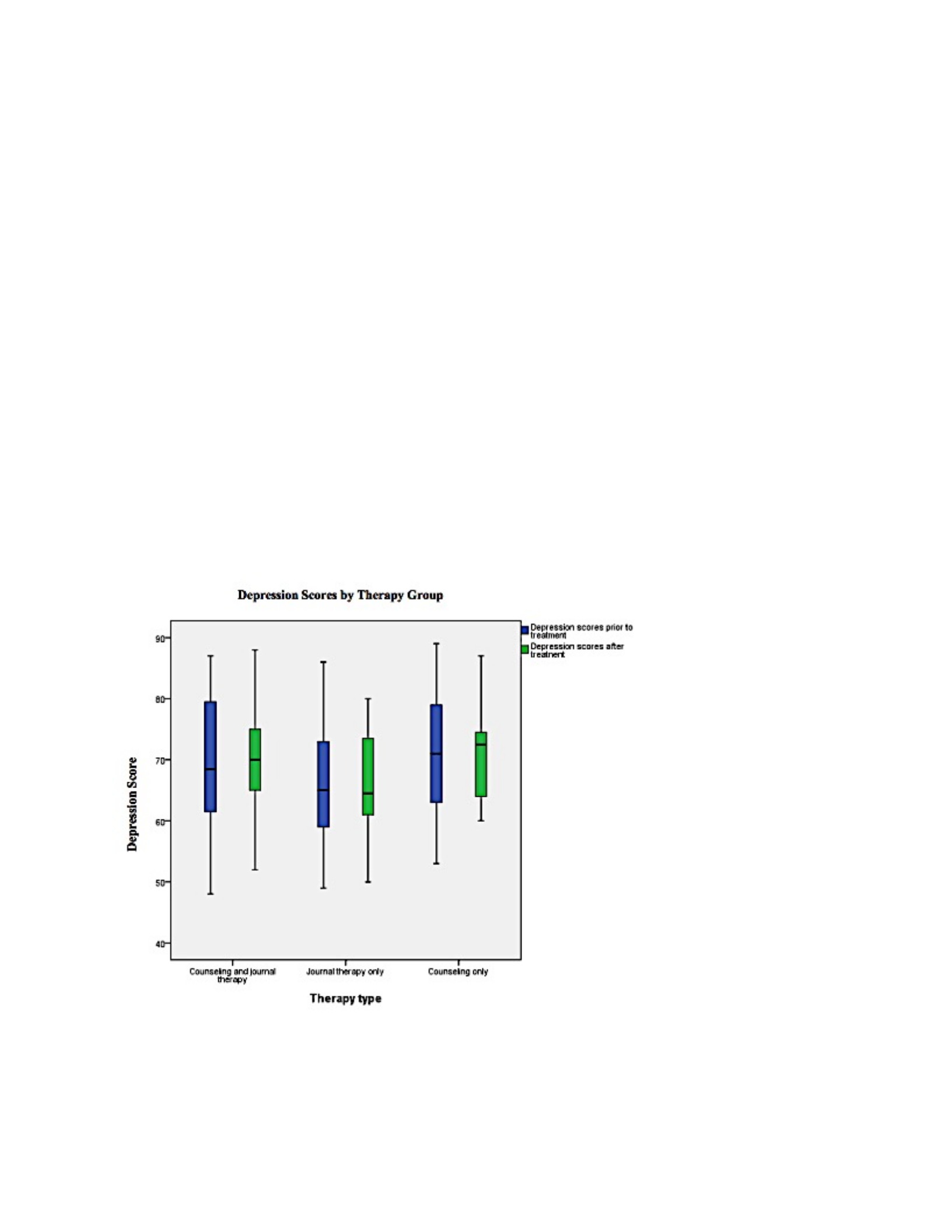
Before further analysis was conducted, the researcher tested for outliers by creating a Box
and Whisker plot of depression scores for each therapy group, both pre-treatment and post-
treatment (see Figure 1). The results indicated that there were no outliers or extreme outliers.
ANCOVA 4
Therefore, the researcher proceeded with the given data.
Figure 1. Box and Whisker Plot for pre-test and post-test scores of counseling and journaling,
journaling only, and counseling only groups.
Assumptions

ANCOVA 5
The ANCOVA test required that the assumption of normality was met (Warner, 2013).
The scores in the test results were shown to be normally distributed for all three groups (p >
0.05) as expressed by the Kolmogorov-Smirnov’s tests of normality (See Table 2). Kolmogorov-
Smirnov was used because the sample size was greater than 50 (n = 60).
Table 2
Kolmogorov-Smirnov Test of Normality
Kolmogorov-Smirnov
Measure group Statistic df Significance
Pre-test JC .12 20 .20
J .09 20 .20
C .10 20 .20
Post-test JC .12 20 .20
J .10 20 .20
C .14 20 .20
Each of these assumptions were tested using a One-Way Analysis of Covariance
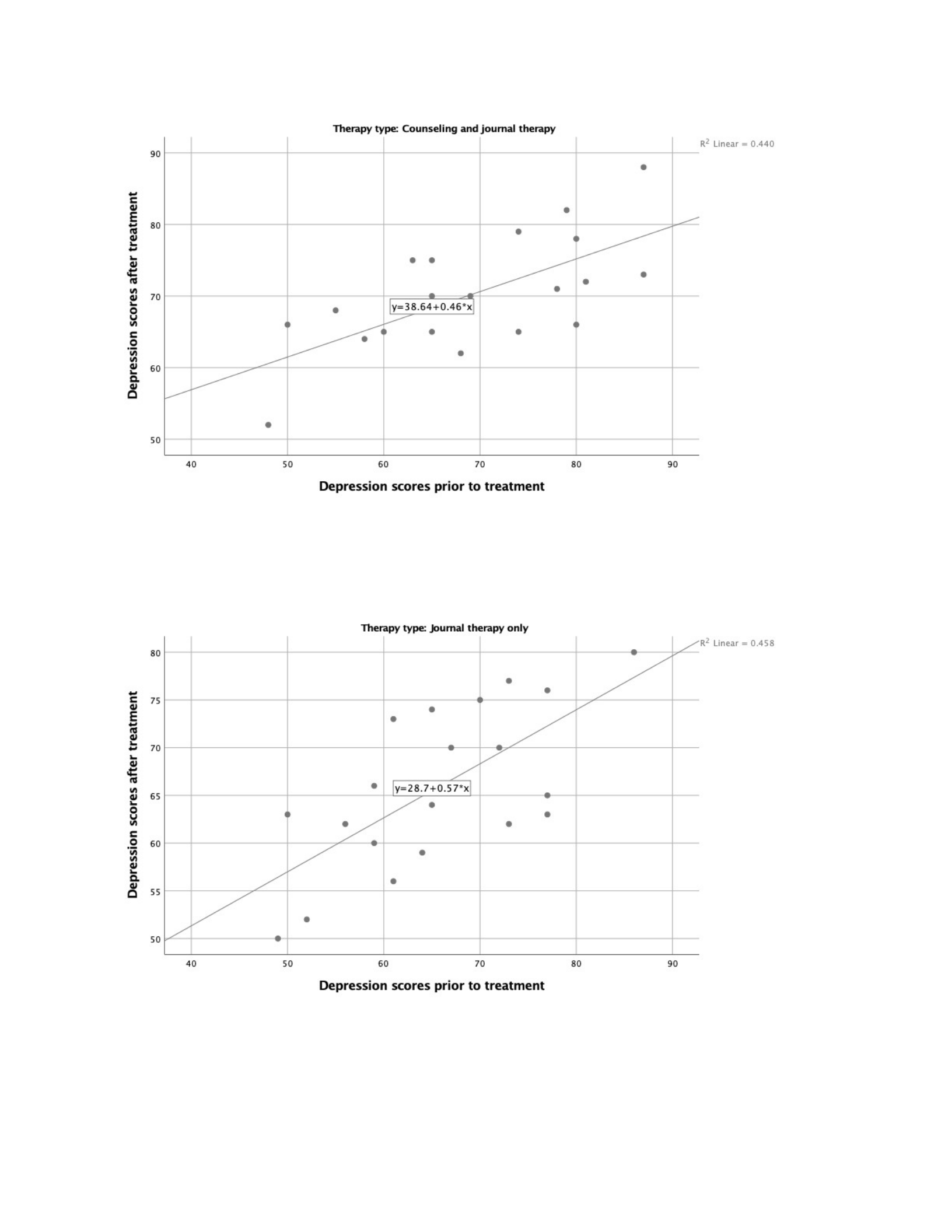
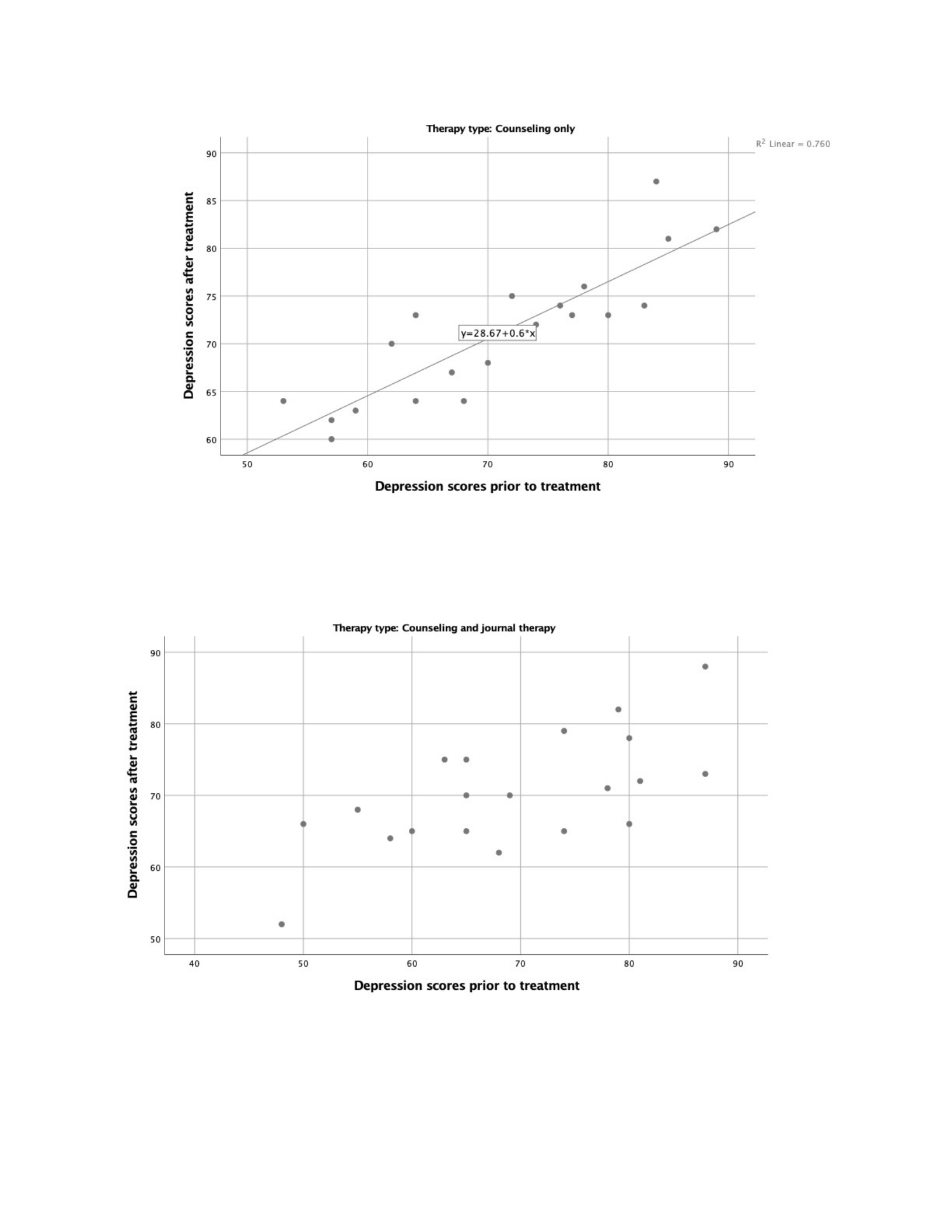
(ANCOVA). Testing started by creating scatter plots between the pre-treatment depression scores
and post-treatment depression scores for each therapy group. A line of fit for each subgroup
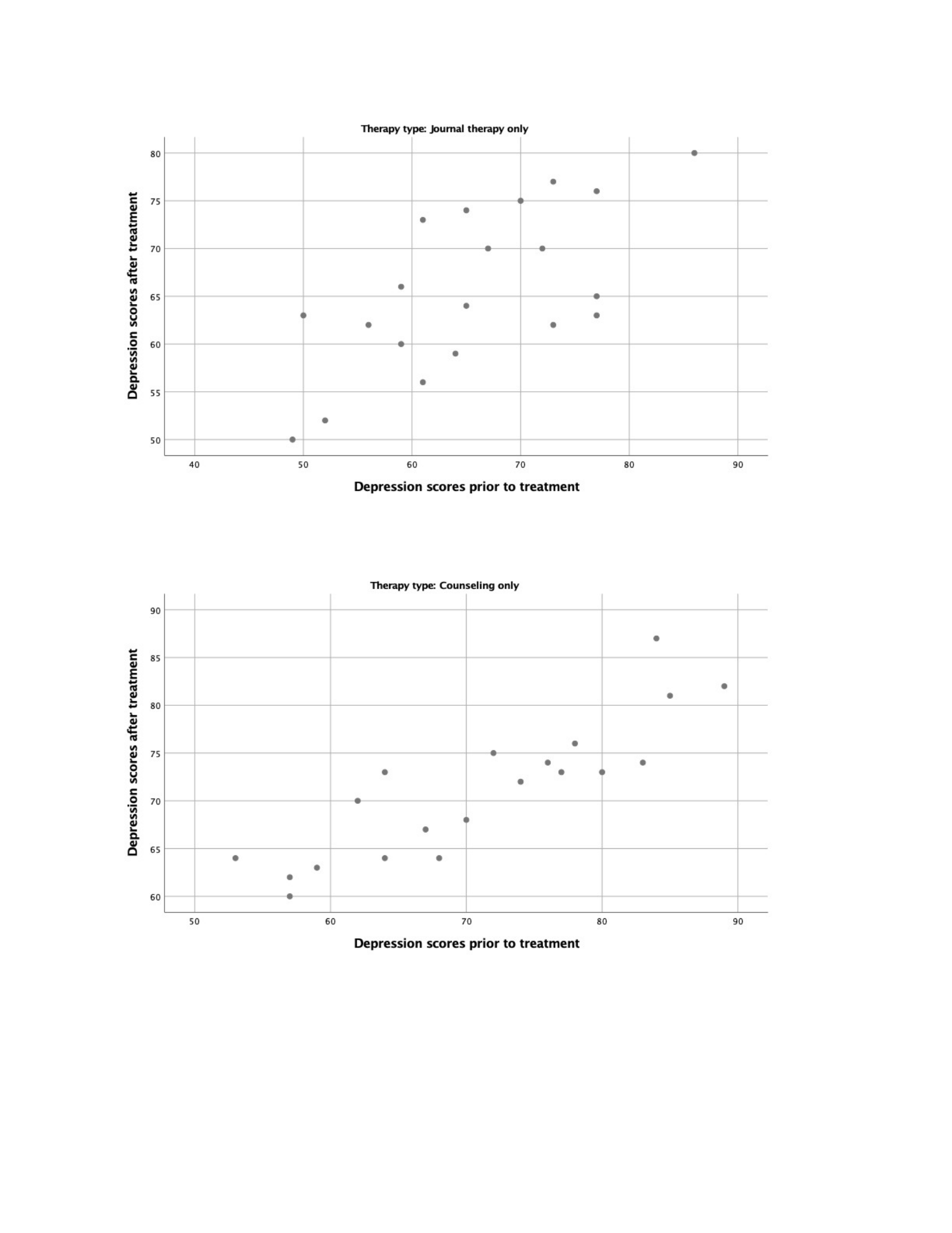
indicated that the assumption of linearity was met (See Figures 2-4). The points clustered around
the line of best fit also revealed an elongated oval shape (or cigar shape), showing that the
assumption of bivariate normal distribution was also met (See Figures 5-6). No outliers were
judged to be extreme.
ANCOVA 6
Figure 2. Linear regression comparing pre-test and post-test scores for counseling and journal
therapy group.
Figure 3. Linear regression comparing pre-test and post-test scores for journal only therapy
group.
ANCOVA 7
Figure 4. Linear regression comparing pre-test and post-test scores for counseling only therapy
group.
Figure 5. Scatter plot comparing pre-test and post-test scores for counseling and journal therapy
group
ANCOVA 8
Figure 6. Scatter plot comparing pre-test and post-test scores for journal only therapy group.
Figure 7. Scatter plot comparing pre-test and post-test scores for counseling only therapy group.
The One-Way ANCOVA requires the assumption of homogeneity of slopes (Warner,
2013). The null hypothesis for this test is that the population effect of the interaction between the

ANCOVA 9
pre-treatment depression scores and therapy groups predicting the post-treatment depression
scores is zero. The results indicated that the interaction was not significant, with F(2, 54) = 0.42,
p = 0.66. As a result, the assumption for homogeneity of slopes was met. See Table 3 for the
Between Subjects Effects
Table 3
Tests of Between-Subjects Effects
Dependent Variable: Depression scores after treatment
Source Type III Sum of df Mean Square FSig. Partial Eta
Squares Squared
Corrected 2213.03a5 442.61 14.58 .00 .57
Model
Intercept 1377.16 1 1377.16 45.36 .00 .46
Group 31.71 2 15.86 .52 .60 .02
Depprior 1885.25 1 1885.25 62.09 .00 .54
Group * 25.69 2 12.84 .42 .66 .02
Depprior
Error 1639.56 54 30.36
Total 290203.00 60
Corrected 3852.58 59
Total
a. R Squared = .57 (Adjusted R Squared = .54)
The One-Way ANCOVA requires the assumption of equal variance (Warner, 2013). The
homogeneity of variance assumption was examined using a One-Way ANOVA Levene’s Test for
the depression scores after treatment. The results indicated a violation F(2, 57) = 5.70, p =
0.006). However, the ANCOVA is considered a robust test against the homogeneity assumption

ANCOVA 10
(Warner, 2013). For this reason, the researcher continued with the analysis. See Table 4 for the
Levene’s Test of Equality of Error Variance
Table 4
Levene’s test of equality of error variance
Levene’s Test of Equality of Error Variance
Measure F df1df2 Significance
Pre-test .36 2 57 .70
Post-test .29 2 57 .75
Results for Null Hypothesis
Since the necessary assumptions were met, a One-Way ANCOVA test was used to test the
null hypothesis that looked at the differences among depression scores for therapy groups while
controlling for pre-test scores. The results showed that group source, JC, C, and J, was not
significant at the α = 0.05 level, F(2, 56) = 1.31, p = 0.28, partial 2 = 0.045. Therefore, the
researchers failed to reject the null hypothesis. The partial eta squared value (2 = 0.045)
indicated a medium effect size (Warner, 2013). See Table 5 Test of Between Subject Effects
Table 5
Tests of Between-Subjects Effects
Dependent Variable: Depression scores after treatment
Source Type III Sum of df Mean Square FSig. Partial Eta
Squares Squared
Corrected 2187.34a3 729.11 24.52 .00 .568
Model
Intercept 1431.66 1 1431.66 48.15 .00 .462

ANCOVA 11
Depprior 1867.30 1 1867.30 62.80 .00 .529
Group 77.75 2 38.87 1.31 .28 .045
Error 1665.25 56 29.74
Total 290203.00 60
Corrected 3852.58 59
Total
a. R Squared = .57 (Adjusted R Squared = .55)
References
Warner, R. M. (2013). Applied statistics: From bivariate through multivariate techniques.
Thousand Oaks, CA: SAGE Publication, Inc.

ANCOVA 12

