


EDUC 812
WRITE-UP: ANOVA WITH TUKEY TEMPLATE
Username: McGraham Anyanwu
Instructions: For this graded assignment, you will complete the write-up below after completing
the corresponding tutorial to this assignment. You will delete figures and tables where appropriate
and then insert correct figures and tables. Also delete and then insert correct answers where there is
RED text.
To begin, cut and paste the data set below into SPSS (or you can type in the data manually). Do
not copy the header row when you paste into SPSS. Before carrying out the analysis in SPSS, you
need to set up your data file correctly using the “Variable View” tab.
Scenario: The purpose of this study was to see if there was a difference in salaries of professors
who teach math (1), science (2), or English (3).
Code Name Subject Salary
1 Williams 1 84000
2 Smith 1 85000
3 Logan 1 95000
4 Alexander 1 75000
5 Oliver 1 87000
6 Daniels 1 87000
7 Jones 2 98000
8 Jefferson 2 85000
9 Madison 2 88000
10 Kelley 2 89000
11 Michaels 2 87000
12 Acara 2 88000
13 Welch 3 65000
14 Christian 3 56000
15 McBride 3 58000
16 Elm 3 57000
17 Toller 3 66000
18 Mason 3 65000

EDUC 812
FINDINGS
Overview
The purpose of this study was to see if there was a difference in salaries of professors who
teach math, science, or English. The independent variable was type of professor and the dependent
variable was salary. A One-way Analysis of Variance (ANOVA) was used to test the hypothesis.
This Findings Section includes the research question, null hypothesis, data screening, descriptive
statistics, assumption testing, and results.
Research Question
RQ: Is there a difference between salaries of professors who teach math, science, or
English?
Null Hypothesis
H0: There is no significant difference between salaries of professors who teach math,
science, or English.
Data Screening
Data screening was conducted on each group’s dependent variable. The researcher sorted
the data on each variable and scanned for inconsistencies. No data errors or inconsistencies were
identified. Box and whiskers plots were used to detect outliers on each dependent variable. One
extreme outlier was identified. See Figure 1 for box and whisker plots.

EDUC 812
Figure 1
Box and Whisker Plots
Descriptive Statistics
Descriptive statistics were obtained on the dependent variable for each group. The sample
consisted of 18 participants. The average salary of a college professor in the United States is
$65,000. Descriptive statistics can be found in Table 1.

EDUC 812
Table 1
Descriptive Statistics
Subject N Minimum Maximum Mean
Std.
Deviation
Math Salary 6 75000 95000 85500.00 6442.049
Valid N (listwise) 6
Science Salary 5 85000 89000 87400.00 1516.575
Valid N (listwise) 5
English Salary 6 56000 66000 61166.67 4622.409
Valid N (listwise) 6
Assumption Testing
Assumption of Normality
The ANOVA requires that the assumption of normality be met. Normality was examined
using Shapiro-Wilks because the sample size was less than 50 participants. The assumption of
normality was met. See Table 2 for Tests of Normality.
Table 2
Tests of Normality
Tests of Normality
Subject
Kolmogorov-SmirnovaShapiro-Wilk
Statistic df Sig. Statistic df Sig.
Salary Math .241 6 .200*.928 6 .566
Science .254 5 .200*.914 5 .492
English .297 6 .108 .808 6 .070
*. This is a lower bound of the true significance.
a. Lilliefors Significance Correction

EDUC 812
Assumption of Homogeneity of Variance
The ANOVA requires that the assumption of homogeneity of variance be met. The
assumption of homogeneity of variance was examined using the Levene’s test. The assumption of
homogeneity of variance was met where (p = .159). See Table 3 for Levene’s test of Equality of
Error Variance.
Table 3
Levene’s test of Equality of Error Varian
Levene's Test of Equality of Error Variancesa,b
Levene
Statistic df1 df2 Sig.
Salary Based on Mean 2.105 2 14 .159
Based on Median 2.170 2 14 .151
Based on Median
and with adjusted df
2.170 2 5.900 .197
Based on trimmed
mean
2.115 2 14 .158
Tests the null hypothesis that the error variance of the dependent variable
is equal across groups.
a. Dependent variable: Salary
b. Design: Intercept + Subject
Results
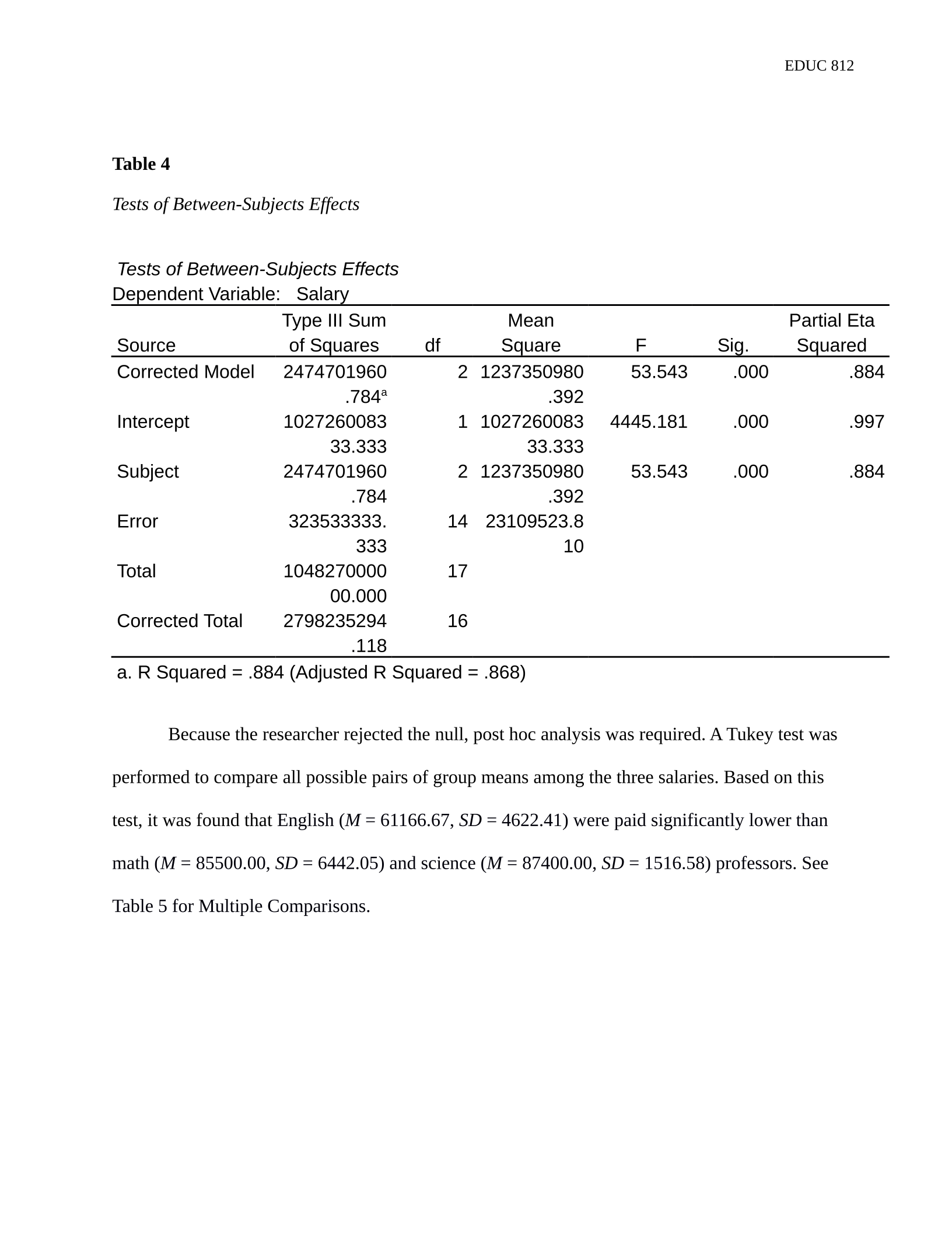
An ANOVA was run to see if there was a difference between salaries of professors who
teach math, science, or English. The independent variable was type of professor and the dependent
variable was salary. The researcher rejected the null hypothesis at the 95% confidence level where
F(2, 14) = 53.54, p = .00. Partial eta square equaled (2part = .884). The effect size was very large.
There was a statistical difference in salaries among math (M = 85500, SD = 6442.05), science (M =
87400, SD = 1516.58), and English (M = 61166.67, SD = 4622.41) professors. See Table 4 for
Tests of Between-Subjects Effects.
EDUC 812
Table 4
Tests of Between-Subjects Effects
Tests of Between-Subjects Effects
Dependent Variable: Salary
Source
Type III Sum
of Squares df
Mean
Square F Sig.
Partial Eta
Squared
Corrected Model 2474701960
.784a
2 1237350980
.392
53.543 .000 .884
Intercept 1027260083
33.333
1 1027260083
33.333
4445.181 .000 .997
Subject 2474701960
.784
2 1237350980
.392
53.543 .000 .884
Error 323533333.
333
14 23109523.8
10
Total 1048270000
00.000
17
Corrected Total 2798235294
.118
16
a. R Squared = .884 (Adjusted R Squared = .868)
Because the researcher rejected the null, post hoc analysis was required. A Tukey test was
performed to compare all possible pairs of group means among the three salaries. Based on this
test, it was found that English (M = 61166.67, SD = 4622.41) were paid significantly lower than
math (M = 85500.00, SD = 6442.05) and science (M = 87400.00, SD = 1516.58) professors. See
Table 5 for Multiple Comparisons.

EDUC 812
Table 5
Multiple Comparisons
Dependent Variable: Salary
Tukey HSD
(I) Subject (J) Subject
Mean
Difference
(I-J) Std. Error Sig.
95% Confidence Interval
Lower
Bound
Upper
Bound
Math Science -1900.00 2910.926 .794 -9518.71 5718.71
English 24333.33*2775.459 .000 17069.18 31597.49
Science math 1900.00 2910.926 .794 -5718.71 9518.71
English 26233.33*2910.926 .000 18614.62 33852.04
English Math -24333.33*2775.459 .000 -31597.49 -17069.18
Science -26233.33*2910.926 .000 -33852.04 -18614.62
Based on observed means.
The error term is Mean Square(Error) = 23109523.810.
*. The mean difference is significant at the .05 level.
Powered by TCPDF (www.tcpdf.org)

