


Running head: COMPARING TWO INDEPENDENT GROUPS
Comparing Two Independent Groups
Belinda Richard
School of Community Care and Counseling- Traumatology
Liberty University

Running head: COMPARING TWO INDEPENDENT GROUPS
Comparing Two Independent Groups – Independent Samples t-test Assumptions
Once surveys have been conducted and data has been gathered, researchers need to
evaluate the significance. As mentioned in previous sections, the goal of surveying is to describe
the population using the sample data. From the sample, statisticians can determine if the mean is
significant in either a positive or negative direction. To do this, a hypothesis is formulated, and
then tests are conducted. In this paper, we will focus on one of these tests, the t-test, specifically
for the difference in means for two groups. Like the t-test for one variable, similar rules apply
when comparing two independent samples and this will be further discussed in subsequent
paragraphs.
As normal with statistical tests, certain conditions need to be met in order to execute. The
assumptions required for an independent samples t-test are: “the measured values in ratio scale or
interval scale, simple random extraction, normal distribution of data, appropriate sample size,
and homogeneity of variance” (Kim & Park, 2019, p. 331). Herzog et al. (2019) define the two
types of variable scales mentioned prior as thus: “Interval: values can be added or subtracted but
not meaningly divided or multiplied” (temperature is an example). “Ratio: values can be added,
subtracted, multiplied, and divided” (weight is an example) (p. 52).
The first of the assumptions essentially requires that the variable be quantifiable; this one
is obvious because statistical techniques cannot be incorporated on categories, we need numbers
to be able to perform calculations. If this is violated, a researcher cannot even formulate a
numerical hypothesis. According to Warner, some researchers are strict about the interval/ratio
requirement, while many researchers are simply okay with quantitative values (p. 257, 2013).
Warner further discusses how means are often calculated from scales and used for comparative

Running head: COMPARING TWO INDEPENDENT GROUPS
analyses, highlighting the superior importance of variables being normally distributed for the
analyses.
Next, it is important for data to be extracted through simple random sampling. Among the
pros of simple random sampling, Sharma lists simplicity, equal opportunity of selection for each
member of the population, unbiasedness, and most importantly, representativeness (2017, p.750).
Consequently, a sample that violates this particular assumption will not be representative of the
intended population, and therefore renders the entire analysis meaningless.
The violation of the normality assumption, like the others, means that are results may not
be an accurate reflection of the population. Kim & Park point out “if the data does not follow the
normal distribution, there is no guarantee that it is centered on the mean” (p. 332). As a result, it
doesn’t make any sense to compare using the mean value. However, this violation is not
regarded as a serious one. Herzog et al. state “As long as the distribution is unimodal, even a
high amount of skew has only a little effect on the Type I error rate of the t-test.” A unimodal
distribution is described by the authors as one that “has only one peak” (p.56). Remember that
the violation of this assumption can often be corrected by transformations.
Recall that the power of a hypothesis test is impacted by sample size, a larger sample size
means more power. Per Banerjee et al. (2009), power is “the probability of observing an effect in
the sample (if one), of a specified effect size or greater exists in the population” (p. 130). Thus, it
goes without saying that a larger sample size is desired. However, different sample sizes for each
of the groups can lead to more problems. Violation of the sample size assumption impacts
power, and by extension affects the ability to capture effects. Kim & Park write “In order to
maximize the power in the t-test, it is most efficient to increase the sample size of both groups

Running head: COMPARING TWO INDEPENDENT GROUPS
equally” (2019, p. 335). Both samples should be the same size to, avoid one sample having more
‘sway’ and to achieve the most reliable results in an independent t test between two groups.
The homogeneity, or equality of variance assumption requires each population to have
the same variance. Per Herzog et al., “Unequal standard deviations, especially combined with
unequal sample sizes, can dramatically affect the Type I error rate. We know that a type I error
happens when you reject a null hypothesis that is true, in essence seeing a relationship that does
not exist, which could have horrific implications in practice. Herzog concludes that both unequal
variances and sample sizes affect the type I error rates.
Type I error rates cannot be discussed without mentioning p-values, since they’re closely
related. Dahiru (2008) describes the p-value to be a probability which takes a value between 0
and 1; furthermore, the closeness of the p value to 0 tells us the strength of its significance (p.
22). Since is a p-value is a probability that can take on any value in that 0 to 1 interval, it is
continuous, and thus cannot practically be zero. Statistical packages often report p-values to a
fixed number of decimal points, making it appear that the p-value is 0. This is untrue (For
example, a p-value of 0.00000234…could show up as 0.0000); however, it is close enough to 0
that the difference is inconsequential.
When it comes to the p-value, our main concern is comparing it to α, the probability of a
type I error. In practice, an α of 5% is most commonly used, but some researchers go as low as
1% for alpha. Even in these cases, as long as p-value is less than α, there’s something statistically
significant going on, and the researcher might be on the way to a discovery.
Comparing Two Independent Groups – Indices on Effect Size

Running head: COMPARING TWO INDEPENDENT GROUPS
While running an independent sample t test, one of researchers’ main interests is to find
the direction of relationships if any exist. In addition to that, it is relevant to know the magnitude.
In fact, a notable number of researchers would agree that this is most important above all. This is
where the indices on effect sizes come into play. We will discuss three of these indices: eta
squared (η2), Cohen’s d, and point biserial correlation coefficient (rpb).
First and foremost, eta squared (η2), similar to r2, is an index ranging from 0 to 1 which
“is an estimate of the proportion of variance in the Y-dependent variable scores that is
predictable from group membership” (Warner, p. 281). According to Tomczak & Tomczak
(2014), this index explains “the percentage of variance in the dependent variable explained by
the independent variable” (p. 22). This is the same as the explanation of the r2, and is calculated
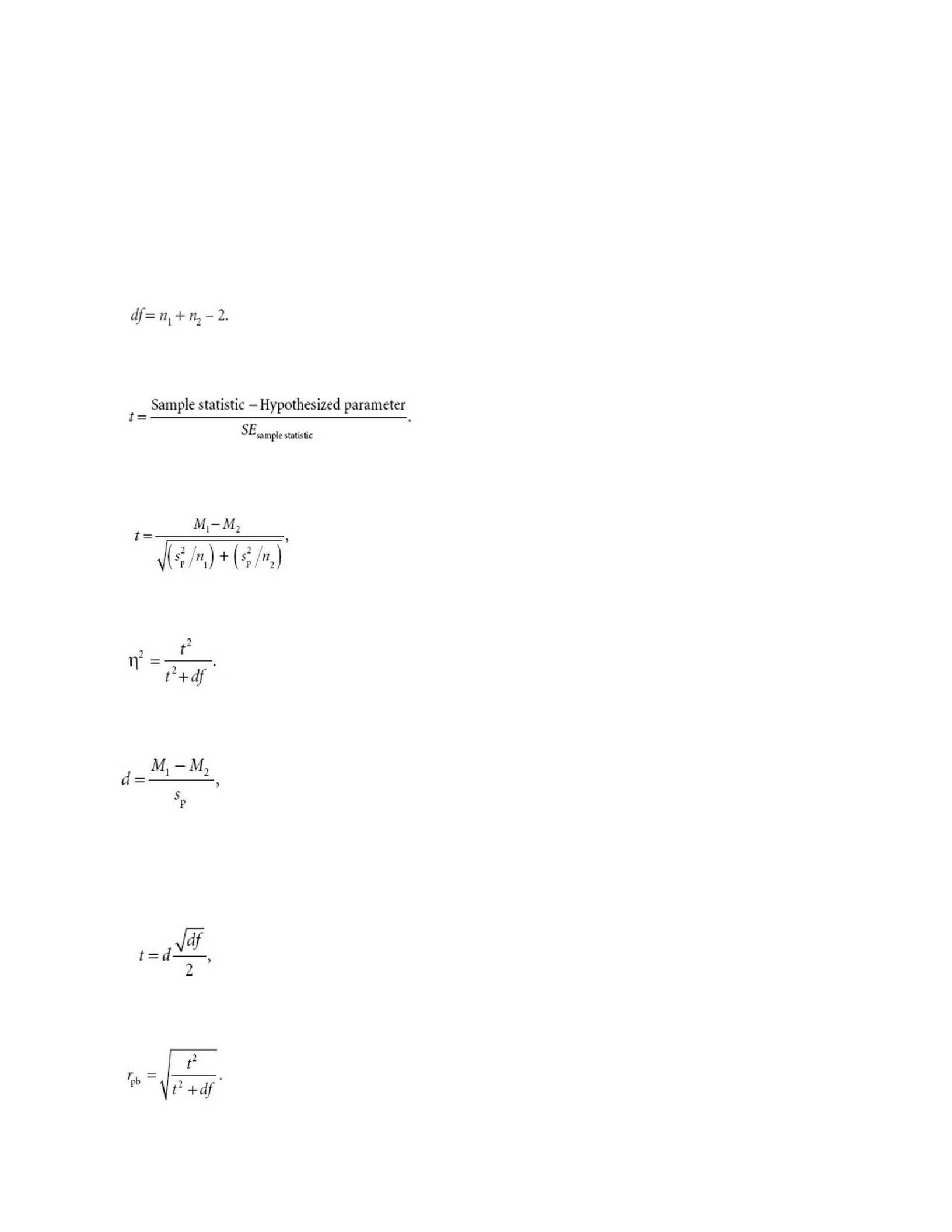
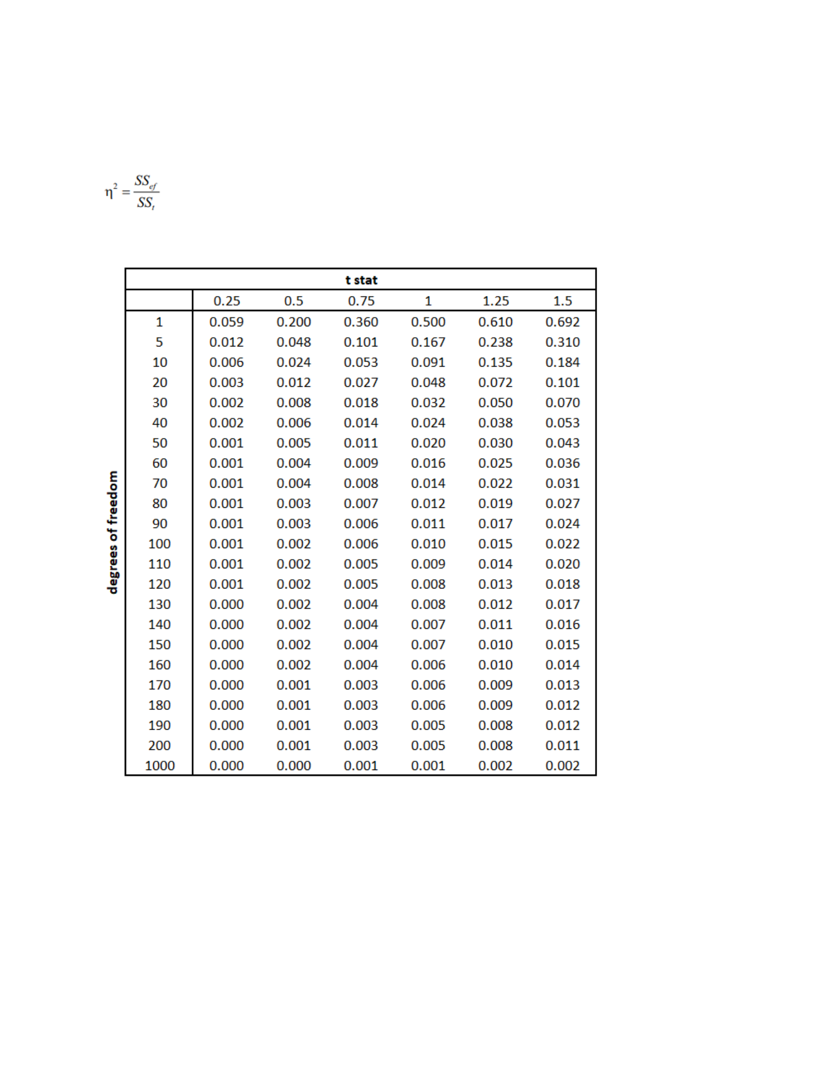
by dividing the sum of squares for the effect by the total sum of squares (Eq 8 in appendix). Per
Serdar, eta squared is good for ANOVA with large samples (2021, p. 8). Another test, which is a
modification of this test exists for smaller samples.
Next up, Cohen’s d, is calculated by subtracting the two means and dividing by the
pooled standard deviation of the difference in sample means (Eq 5 in appendix). Per Warner, a
large number is desirable, and indicates a large effect compared to the noise (other uncontrolled
effects); furthermore, it is good for “visualizing how much overlap there was between the
distributions of scores in the two groups” (p. 282). A larger value would imply that the
relationship been explored is more likely significant. Serdar describes Cohen’s d as being
generally good for t tests with means (2021, p. 8). This test is quick and easy to execute, and also
has easily interpretable results.

Running head: COMPARING TWO INDEPENDENT GROUPS
Lastly, a point bi-serial correlation also ranges from 0 to 1. It is calculated as the square
roof of the t stat squared divided by t squared + degrees of freedom. Warner notes that it’s best
used “when results of studies that involve comparisons between pairs of group means are
combined across many studies using meta-analytic procedures” (p. 283). From the formulas in
the appendix, it’s apparent that the point bi-serial correlation is essentially the square root of the
eta squared. Thus, a very large effect of .6 in terms of the point bi-serial correlation would
be .360 in terms of the eta squared. Another author recommends the point bi-serial r when one
variable is a true dichotomy and the other is a quantitative interval/ratio (Warner, p. 431).
Three factors that influence the size of t include the size of the difference in means, the
sample size of the study and the amount of variation present in the study. Per Warner, all other
variables constant, the sample size of both variables increasing cause the t ratio to do the same
(p. 279). A large t ratio “is most likely to occur in a study where the between-group dosage
difference, indexed by M1 − M2, is large; where the within-group variability due to extraneous
variables, indexed by s2p, is small; and where the ns of subjects in the groups are large” (p. 279).
Looking at Eq 1 and Eq 4 in the appendix, it can be observed that increases in sample
sizes (n1, n2) would lead to increases in eta squared. This is true since eta squared depends on t
and degrees of freedom, and the latter depends on the sample sizes. However, a large eta squared
effect (such as eta squared =.64) could still be achieved with a small t ratio; for this to be the
case, sample sizes and the differences between groups (M1 – M2) would need to be small, and
the pooled variance between the samples would need to be large as well. Both Fig 1 as well as
Eq 3 in the appendix illustrate this; thus, it is possible to have a high eta squared and a t value

Running head: COMPARING TWO INDEPENDENT GROUPS
that is statistically insignificant. This just highlights how analyses can be manipulated in several
ways.
In summary, holding all other variables constant, an increase in M1 – M2 increases t, an
increase in the pooled variance reduces t, and an increase in n increases t. These findings
emphasize the need of researchers to be careful with the way studies are structured and defined.

Running head: COMPARING TWO INDEPENDENT GROUPS
References
Warner, R. M. (2013). Applied statistics: From bivariate through Multivariate Techniques.
SAGE Publications.
Kim, T. K., & Park, J. H. (2019). More about the basic assumptions of t-test: normality and
sample size.RKorean journal of anesthesiology,R72(4), 331-335.
Herzog, M. H., Francis, G., & Clarke, A. (2019). Variations on the t-Test. InRUnderstanding
Statistics and Experimental DesignR(pp. 51-59). Springer, Cham.
Sharma, G. (2017). Pros and cons of different sampling techniques.RInternational journal of
applied research,R3(7), 749-752.
Banerjee, A., Chitnis, U. B., Jadhav, S. L., Bhawalkar, J. S., & Chaudhury, S. (2009). Hypothesis
testing, type I and type II errors.RIndustrial psychiatry journal,R18(2), 127-131.
Dahiru, T. (2008). P-value, a true test of statistical significance? A cautionary note.RAnnals of
Ibadan postgraduate medicine,R6(1), 21-26.
Tomczak, M., & Tomczak, E. (2014). The need to report effect size estimates revisited. An
overview of some recommended measures of effect size.RTrends in sport
sciences,R1(21), 19-25.
Serdar, C. C., Cihan, M., Yücel, D., & Serdar, M. A. (2021). Sample size, power and effect size
revisited: simplified and practical approaches in pre-clinical, clinical and laboratory
studies.RBiochemia medica,R31(1), 27-53.
Running head: COMPARING TWO INDEPENDENT GROUPS
Appendix
Eq 1 (Warner, 2013, p. 268):
Eq 2 (Warner, 2013, p. 270):
Eq 3 (Warner, 2013, p. 275):
Eq 4 (Warner, 2013, p. 281):
Eq 5 (Warner, 2013, p. 282):
Eq 6 (Warner, 2013, p. 283):
Eq 7 (Warner, 2013, p. 283):
Running head: COMPARING TWO INDEPENDENT GROUPS
Eq 8 (Tomczak & Tomczak, 2014, p. 22):
Fig 1 (Computation of eta squared based on different t-stats and sample size combinations):
Note: These are hypothetical numbers just to illustrate the relationship.

