


BRIEF INTRODUCTION TO GRAPHS
A formal introduction to graphs may be found in most
discrete math textbooks. The purpose of this section is not
to provide such an introduction. Rather, we will focus more
on the data structures used to represent graphs and the
algorithms associated with them. Regardless, some basic
vocabulary will prove useful.
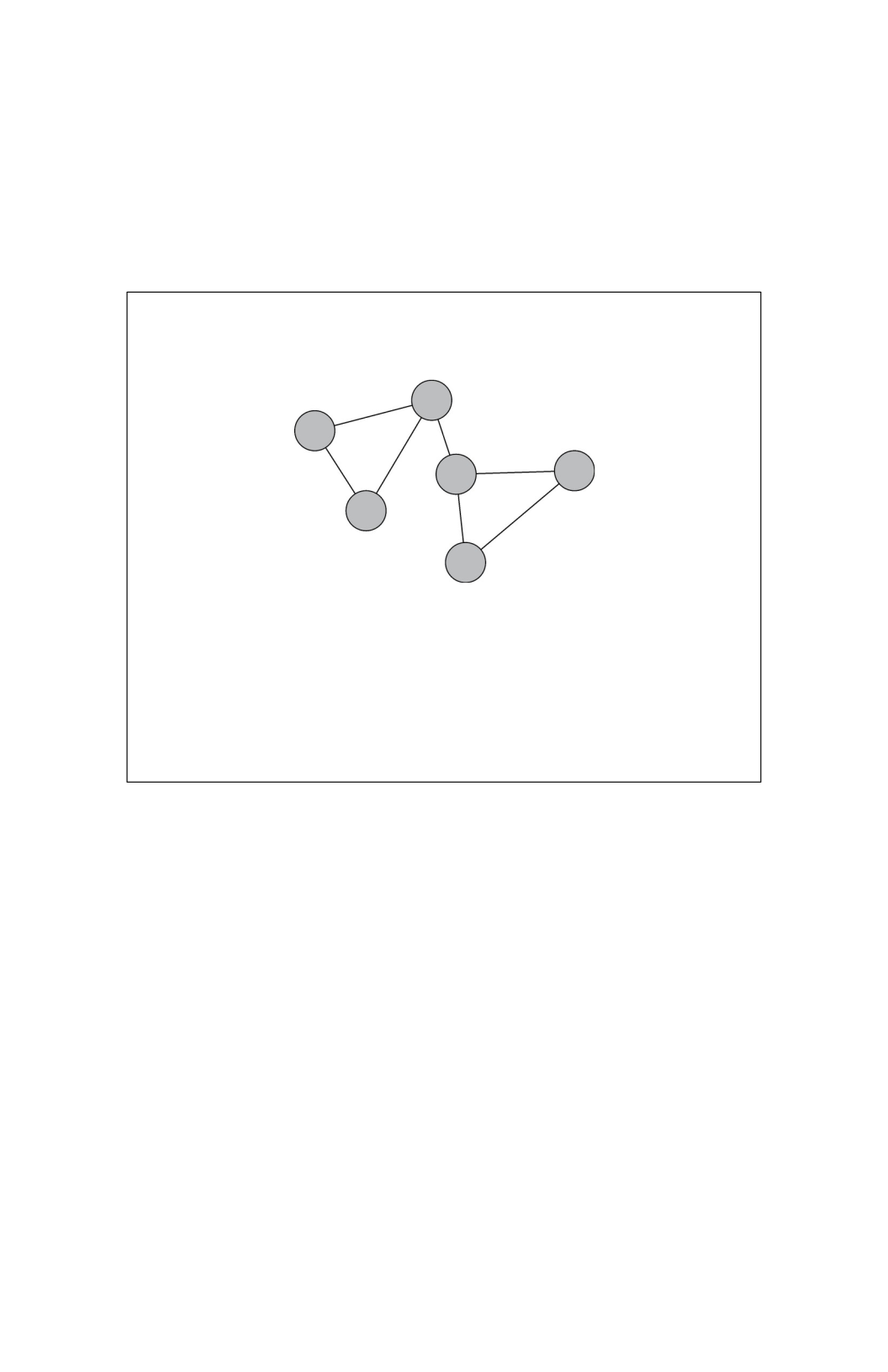
Nodes are the primary objects under consideration
in graphs. They are associated with other nodes by means
of edges. Each edge is incident to two nodes. We define
adjacent nodes of a given node as alternate nodes of
incident edges. Adjacent nodes are sometimes referred to
as neighbors. The degree of a node is the number of its
incident edges or adjacent nodes (not including the node
itself). Our depiction of graphs will look much like our
depiction of trees. This should come as no surprise
because, if you recall, trees are a special case of graphs.
If you cross-reference this chapter against more
mathematically focused textbooks (which is strongly
encouraged), you will find that some of these definitions
vary. In particular, mathematical textbooks typically refer
to nodes as vertices. They are also more precise in
mathematical notation. For example, this chapter will use
the symbol N to denote the number of nodes in the graph.
In a mathematics context, the set of nodes is represented
as set V and the number of nodes as
|V|
(or the cardinality
of V).
Paths and cycles will play a large role in our graph
algorithms. A path is some sequence of edges that
allows you to
travel from one node to another. A cycle is a path that
starts and ends at the same node. Sometimes cycles are
useful, but they often represent challenges in graph
algorithms. Failing to detect a cycle in graph algorithms
often results in implementations falling into endless loops.
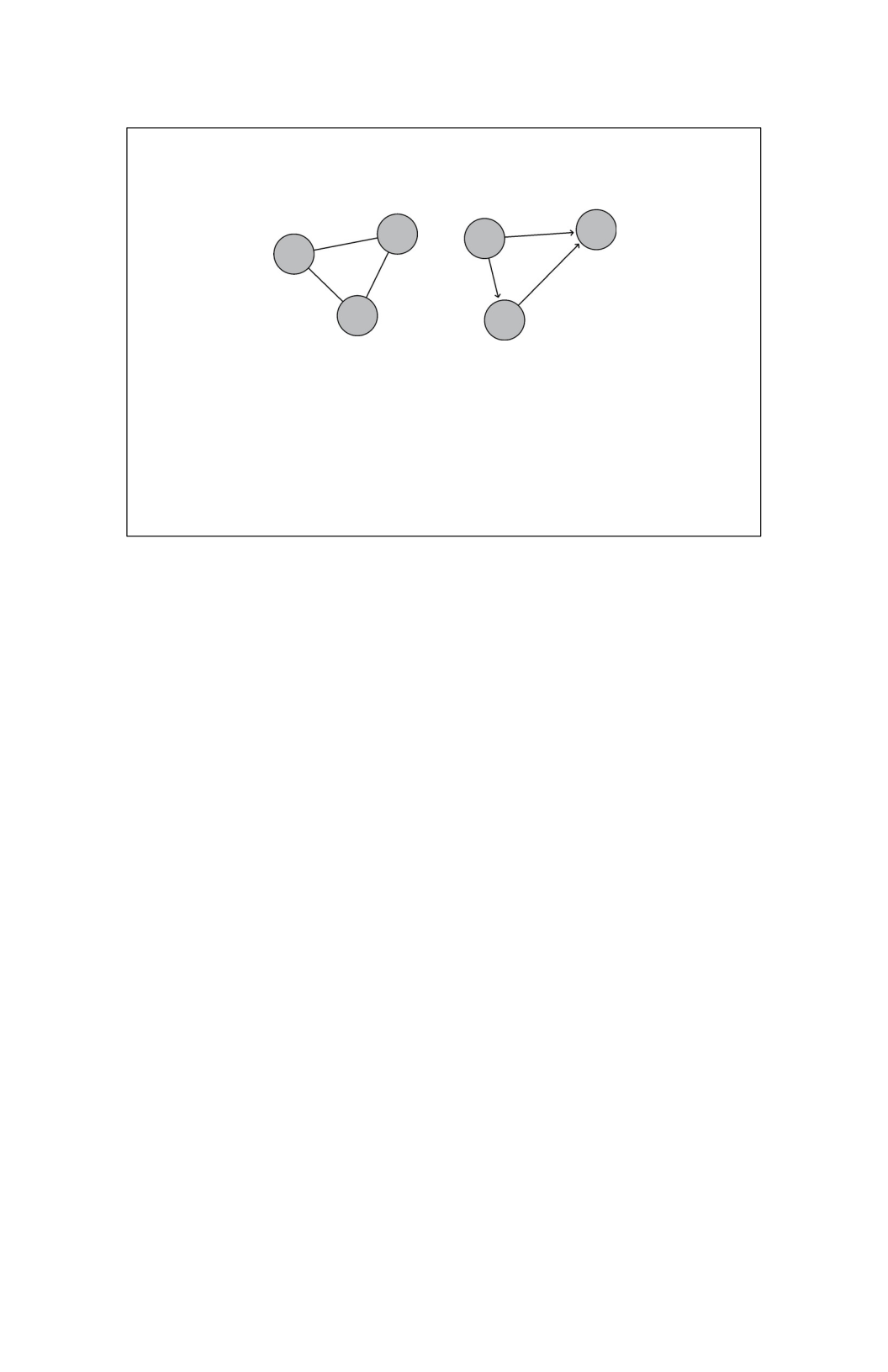
We will often need to consider whether a graph is
directed or undirected. A directed graph is one in which
each edge goes in a single direction. A network of flights
across the United States is probably directed because
every flight from city A to city B does not necessarily have
a flight back from city B to city A. An undirected graph
implies that we could traverse each edge in either
direction. A network of roads between towns is likely
undirected because most roads permit travel in both
directions. If you reframe the network of roads, you could
describe each lane as an edge, resulting in a directed
graph. In our visual depictions of graphs, you will know
whether a graph is directed or undirected by the use of
arrows. Of the graphs below, the left graph represents an
undirected graph, and the right represents a directed
Figure 11.1

graph:
Another distinction we make will be between
weighted and unweighted graphs. Weighted graphs have a
numerical value associated with each edge, which
represents the weight of that edge. For example, roads
between cities have distances, and computer networks
have measures of latency. Some graphs have no
meaningful numerical value for edges and are considered
unweighted. For example, social networks may have no
meaningful weight for the relationship between two
people. Much of this chapter will focus on graphs that are
both weighted and directed.
Representations of Graphs
In a discrete math class, these graphs would be
represented with basic set notation. We, however, have
the additional burden of needing to represent this in a
machine-readable format. Two main strategies exist for
representing graphs in data structures, but there are
numerous variations on these. We may choose to modify
or augment these structures depending on the
Figure 11.2

specific problem,
language, or computing environment. For simplicity, we
will only address the two main strategies.
Adjacency
Matrices
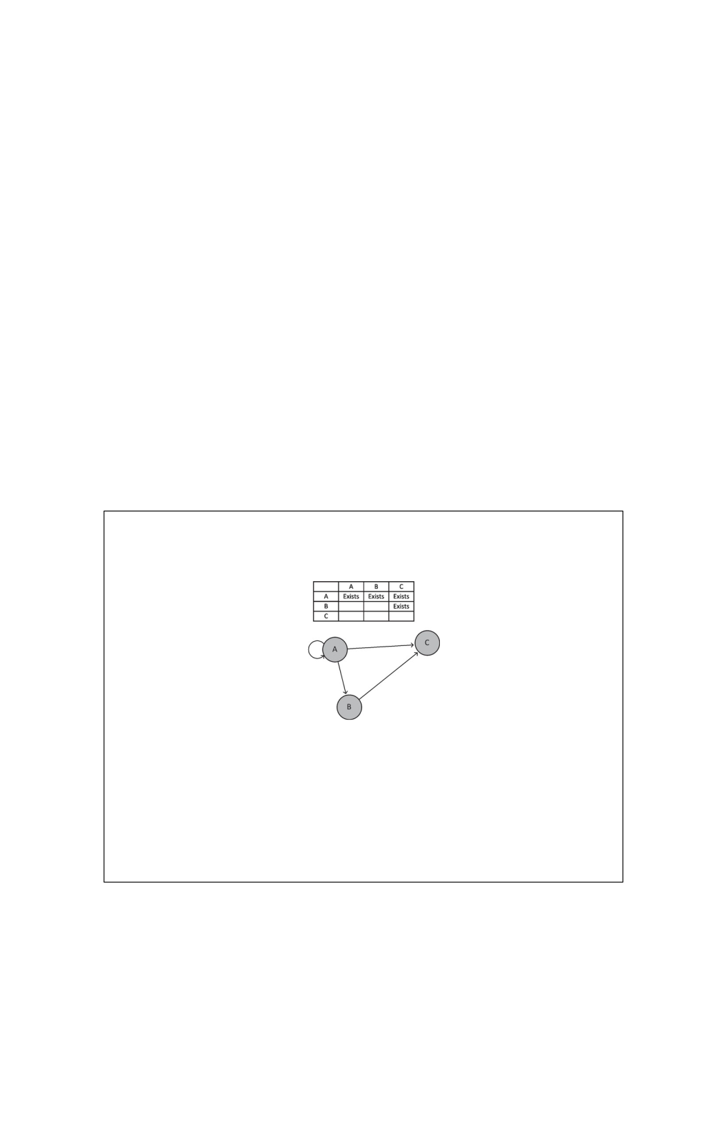
An adjacency matrix is typically conceptualized as a table
where the count of both rows and columns is equal to the
number of nodes in the graph. Each row is assigned a node
identifier, and each column is also assigned a node
identifier. To determine whether an edge exists from node
A to node B, we find the row for A and cross- reference B.
The information in that cell of the table then provides
information regarding the nature of the edge from A to B.
Consider the following example:
Notice that all we have asserted so far is that the
intersection of the row and column supplies information about
the
nature of the edge. The data we store at each
intersection
depends
Figure 11.3

on the type of graph we are modeling. Some
considerations for adjacency matrices include the
following:
•
Weighted or Unweighted: If the graph is weighted,
intersections will store the weight of the edge as
some
numeric type. In unweighted graphs, the
intersection simply
stores whether the edge exists.
•
Directed or Undirected: If the graph is undirected,
each nondiagonal intersection stores redundant
information with exactly one other cell. For example,
if an undirected graph has an edge between A and B,
then the (A, B) intersection stores the same
information as (B, A). On occasion, this may be
desirable or undesirable. Naturally, a directed graph
would store nonredundant information in each cell.
•
Node Identities: The most logical choice for an
underlying data structure would be a two-dimensional
array. To leverage the constant-time lookups, we must
provide an integer identifier for each node.
•
Existence of Edges: Regardless of the points above, we
must determine how to indicate that no edge exists.
While many modern languages have some concept of
a nullable type, you may not always want to use it.
Particularly, nullable types often come with an implied
increase in storage size (it may take 32 bits to store an
integer, but storing an integer along with whether it
exists is more information and consequently more
bits). As a result, we might, by convention, choose a
value to store in the matrix that indicates that no edge
exists. Most weighted graphs in the natural world have
strictly positive weights, so storing a −1 may serve as
a useful indicator for a nonexistent edge. When
working with an unweighted graph, simple 0s and 1s
or true and false will suffice.
Adjacency
Lists
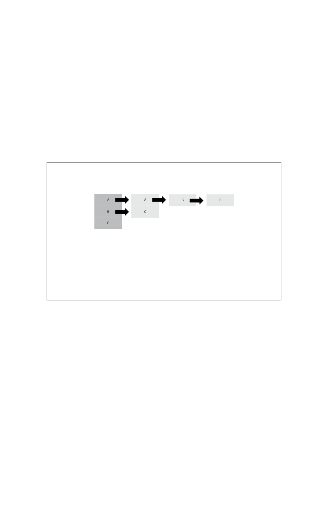
If we perceive an adjacency matrix as a square table of
edge information, an adjacency list is a jagged list of lists.
The primary list has one entry for each node in the graph.
Each of those entries then points to a list of adjacent
nodes. The size of each secondary list depends on the
degree of that node. Using the same graph as we used for
adjacency matrices, we have the following adjacency list.
This is how adjacency lists are often portrayed
visually, but we should note that the word “list” is in
reference to the abstract data type list rather than a linked
list. Also note that while the primary list clearly stores
nodes, the secondary lists effectively store edges.
The list of lists nature of adjacency lists may be
implemented in numerous ways. Considerations for
concrete implementations include the following:
•
Weighted or Unweighted: Weighted graphs require
each entry in the secondary lists to store both the
adjacent node’s identity and that edge’s weight. For
this reason, we cannot store simple primitive types in
each secondary entry. This implies that we
Figure 11.4

will likely need some kinds of composite types such as
objects or structs. Unweighted graphs are easily stored
using the identity of the node and may not require
additional types.
•
Directed or Undirected: As with adjacency matrices,
undirected graphs tend to lead toward redundancy in
data. If an undirected graph has an edge between A
and B, then A’s secondary list stores a reference to B,
and B’s secondary list stores a reference to A. Directed
graphs have no such concern.
•
Underlying Data Structures: As with adjacency
matrices, it may be convenient to identify each node
using an integer. This allows us to leverage constant-
time lookups when looking for nodes in primary or
secondary lists. Unlike adjacency matrices, using
arrays for secondary lists may pose additional
challenges if edges are frequently added or removed
(due to the fixed size of arrays).
Algorithms
Much like our discussion of trees, graph algorithms could
consume chapters of a textbook. Rather than a broad
survey of problems and known algorithms, we will address
only three specific problems.
Traversal
Two frequent questions with graphs are (1) how we can
visit each node and (2) if we can find a path between two
nodes. They arise whenever we want to broadcast on a
network, find a route between two cities, or help a virtual
actor through a maze. We rely on two related algorithms to

accomplish this task: breadth first traversal and depth first
traversal. If we wish to perform a search, we simply
terminate the traversal once the target node has been
located.
Both algorithms depend on knowing some start
node. If we are attempting to traverse all nodes, a start
node may be chosen arbitrarily. If we wish to find a path
from one node to another, we obviously must choose our
start node deliberately. Both algorithms work from the
same basic principle: if we wish to visit every node
originating from some start node, we first visit its
neighbors, its neighbors’ neighbors, and so on until all
nodes have been visited. The primary distinction between
both is the order in which we consider the next node.
Breadth first spreads slowly, favoring nodes closest to the
start node. Depth first reaches as deep as possible quickly.
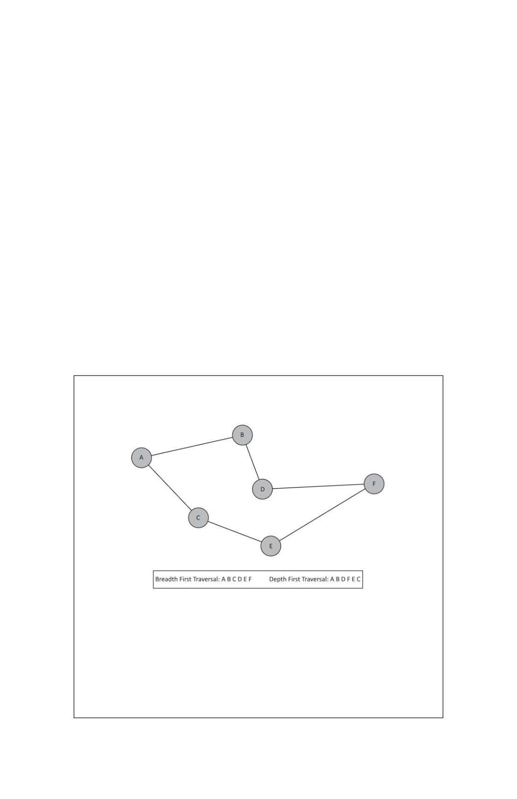
Below are examples of both traversals. Note that there is
no unique breadth first or depth first traversal, but
rather they are dependent on a precise implementation.
The examples below represent possible traversals. There
are other possibilities.
Figure 11.5

Note the difference in these traversals. Because breadth
first starting from A will consider all A’s neighbors first, we will
encounter C before we encounter F. Depth first will
instead prioritize B’s neighbors before completing all of A’s
neighbors. As a result, depth first reaches F before breadth
first does.
In addition to the order in which we visit neighbors,
we must also pay close attention to cycles. Recall that
cycles are paths that start and end at the same node. In
the depth first example
above, what happens when we
finally visit C only to find its neighbor
is A? If we fail to
recognize this as a cycle, we will again traverse A B D F E
C and continue to do so indefinitely. We must avoid visiting
already visited nodes. We will need to incorporate this into
the algorithm as well.
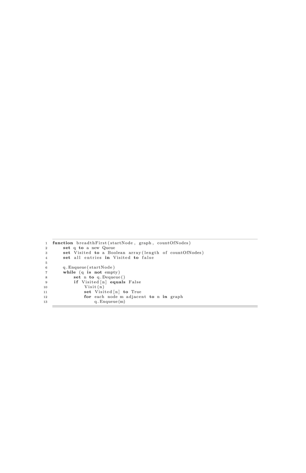
Below is the pseudocode for a breadth first
traversal. The function call Visit is simply a placeholder for
some meaningful action you might take at each node (the
simplest of which is simply printing the node identifier). It
also assumes that node identifiers are integers.
Consider the above pseudocode along with figure
11.5. Assume a mapping from the letters A–F to integers 1–
6, respectively. We first enqueue A. The queue is not
empty, so we dequeue A. We have not yet visited it, so we
visit, mark as visited, then enqueue the neighbors (B and
C). In the case of breadth first, these two nodes were
enqueued before D, E, and F. As a result, B and C will be
visited before D, E, and F.
Also note the utility of the visited array. We visit a node,

mark it as visited, then enqueue its neighbors. Once we
have visited a node and enqueued its neighbors, the
conditional on line 9 will prevent us from doing the same
again. This is our mechanism for avoiding cycles.
This pseudocode describes a breadth first traversal
but only requires a nominal change to make it a depth first
traversal. Recall that after we visited A, we visited B and C.
This was due to the first-in-first-out nature of queues.
Consider what happens if we swap our queue for a stack.
We visit A and now push B and C. C was the last node
pushed, so a pop returns it. We then push A and E, which
will eventually be popped before B. As a result, we
prioritize nodes deep in the graph before ever considering
B. In fact, we eventually consider B due to its adjacency to
D rather than its adjacency to A.
Three aspects of graph algorithms make runtime
analysis difficult. Because of these challenges, runtime
analysis in this chapter will be less precise than in others
but still descriptive as to roughly how much effort is
required to perform the task at hand.
•
We are typically working with two variables: count of
nodes and count of edges. In the case of breadth first
traversal, we can see that we will only visit each node
once. We also enqueue and dequeue once for each
edge (plus an additional enqueue/dequeue for the
start node). This gives us a runtime of O(N + E),
where N is the number of nodes and E is the number
of edges.
•
Analysis can be confusing because the upper bound of
E is O(N
2
). An explanation of why can be found in
Discrete Mathematics: An Open Introduction (found in
the references for this chapter). There the author
explains how the number of edges in a complete graph
relates to the number of nodes. The explanation
closely resembles the justification for O(N
2
) runtime of
selection and Insertion Sort. Because of these two
aspects, we can correctly say O(N+E) or O(N
2
), the
choice of which is typically dependent on the current

context. If we

know that the number of edges is relatively low
compared to the number of nodes, then use the sum of
the two. If we know the graph to be highly connected,
it is better to recognize the runtime as quadratic.
•
Algorithms are typically presented conceptually
without regard to precise implementations of graphs or
auxiliary data structures. For example, if we are
working in an object- oriented system, we may
leverage adjacency lists, which limit our ability to
perform constant-time indexing into the adjacent
nodes. If we have no mapping from nodes to integers,
we may have to perform Linear Searches to determine
if nodes have been visited.
Single Source Shortest Path
While breadth first and depth first searches provide a
path from a source to a destination, they do not guarantee
an efficient path. Accomplishing such a task requires that
the algorithm consider the weights of the edges that it
traverses as well as the cumulative weights of edges
already traversed. Numerous algorithms exist to find the
shortest path from one node to another, but this section
will focus on Edgar Dijkstra’s algorithm.
Dijkstra’s algorithm determines the shortest path
between a source and destination node by maintaining a
list of minimum distances required to reach each node
already visited by the algorithm. It is an example of a
greedy algorithm. This is a general strategy employed in
algorithms, akin to the divide-and-conquer strategy
employed in Binary Search or Merge Sort. Greedy
algorithms make locally optimal choices that trend toward
globally optimal solutions. In the case of Dijkstra’s (and
Prim’s to follow), we only consider a single node at a time
and use the information at that location in the graph to
update the global state. If we carry this strategy out in

clever ways, we can indeed determine the shortest
path between two nodes without each step considering the
entire graph.
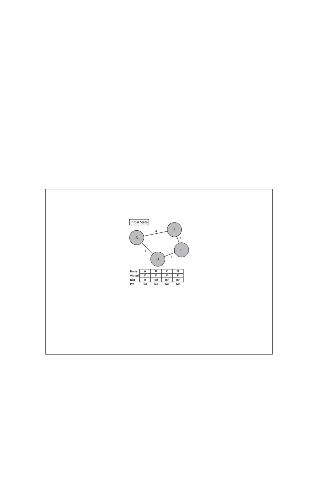
In the following graph, consider finding the
shortest path
from A to D. Note that in the initial state, we
acknowledge that the
distance from the source node to
itself is 0. This is analogous to enqueuing or pushing the
source node in breadth first and depth
first traversals. The
primary control flow will again be a loop, which
selects the
next node to consider. Initializing some state again
provides the loop with a logical place to begin. Also note
that we maintain predecessors for each node whenever
we update the
distance to that node. This helps traverse the
shortest path after the
algorithm has been completed.
Now that we have some predefined state, we will
begin our iteration to update the distance and predecessor
arrays with the best information we know so far. Given the
nodes we have visited so far (namely, A), we know we
can reach B with a weight of 4 and predecessor node A.
We can also reach C with weight 6 and predecessor node
A. Note here that we are not claiming that the edge AB is
the shortest path from A to B or that AC is the shortest
Figure 11.6
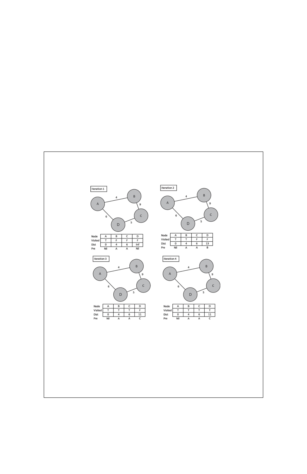
path from A to C. What we are claiming is that of the nodes
visited so far, the minimum weight paths to B or C are 4
and 6, respectively. We then start the next iteration by
carefully choosing the next node to visit. It should be one
that has not yet been visited so that we do not create
cycles. Additionally, regarding the shortest path, we must
choose the next node based on which has the minimum
distance from the starting node. We then repeat this
process until each node is visited or we reach some
desired destination node.
Figure 11.7
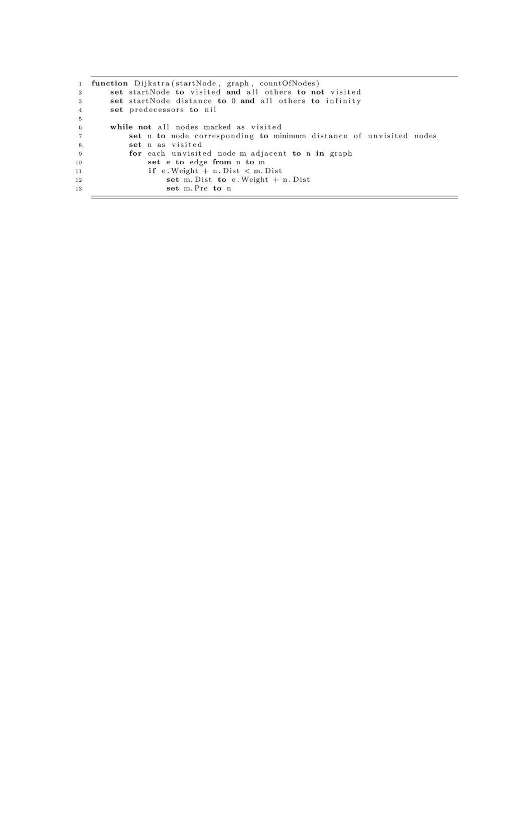
As with breadth first and depth first traversals, the
precise runtime cannot be determined without specifying
exactly how visited, distance, predecessors, and edges are
structured. What we can determine with certainty is that
the while-loop will iterate the same number of times as the
number of nodes in the graph. This is evident because
each iteration marks a node as visited, and the loop
terminates when all nodes are visited. Assuming we are
looking for all shortest paths (or our destination node is the
last to be visited), we will perform the body of the inner
loop once for each edge in the graph. This very closely
approximates the runtime behavior of the traversal
algorithms earlier and results in a likely worst-case runtime
of O(N
2
). However, Dijkstra’s algorithm is well researched,
and known improvements can be made to this runtime by
choosing clever data structures to represent different
components.
Minimum Spanning Trees (MSTs)
A Minimum Spanning Tree (MST) is a subgraph (subset of
edges) that
satisfies the following conditions:
1.
It must be a tree. In other words, there must be
no cycles within the subgraph.
2.
It must be spanning, which means that all the nodes

in the original graph exist in the subgraph and are
reachable using

only the edges in the subgraph.
3.
It is possible to have more than one spanning tree for
a given graph. Of those possible spanning trees, the
MST is the one with the lowest cumulative edge
weight.
As with other graph properties and algorithms,
MSTs have numerous applications in the natural world. The
canonical example is that of a network broadcast. Imagine
computers as nodes and the network connections
between them as edges. In computer networking, we often
want to be able to broadcast a message to all nodes on the
network (or, put simply, ensure that all nodes receive a
particular message). The MST represents the lowest-cost
means of transmitting such a message. Note that this is
not the fastest means of transmission. That would indeed
be a tree created by running a single-source shortest-path
algorithm like Dijkstra’s.
As with single-source shortest path, MSTs can be
produced via numerous algorithms. The only one we
address here is Prim’s. We do so due to its similarity with
Dijkstra’s. Dijkstra’s produced shortest paths by comparing
a known distance against the sum of the cumulative
distance to the predecessor plus the newly considered edge
(see line 11 in the pseudocode). This comparison can be
made because the distance for a node denotes the
shortest path we have considered so far. Prim’s algorithm
changes the meaning of the distance value as well as
the comparison on line
11. Rather than representing the cumulative distance as we
did for shortest path, distance now represents the cost to
add that node into the MST. The final change is simple: if we
remove n.Dist from both lines 11 and 12, then we now
find the MST rather than a shortest-path tree.
Everyone in life faces hard problems. Figuring out what to
do with your life or career can be hard. You may find it
hard to choose between two delicious menu items. These
problems, while “hard” in their own way, are not the kinds

of hard problems we will be exploring in this chapter. In
this chapter, we will introduce some
of the key ideas that
support the theory of computation, the theoretical
foundation of computer science. The discovery of these

concepts is rather recent in the history of science and
mathematics, but these concepts provide some fascinating
insight into how humanity may attempt to solve the most
difficult problems.
In the following sections, we will introduce the most
discussed complexity classes in theoretical computer
science. These are the complexity classes of P, NP, NP-
complete, and NP- hard. These classes highlight many
interesting and important results in computer science. We
will explore what makes problems “easy” or “hard” in a
theoretical sense. We will then explore some concepts for
tackling these hard problems using approximations and
heuristics. Finally, we will end the chapter with a
discussion of an “impossible” problem, the halting
problem, and what this means for computability.
The goal of this chapter is to simply introduce some
of the important theoretical results in computer science
and to highlight some ways in which this knowledge can be
practical to a student of computer science. We will not
introduce a lot of formal definitions or attempt to prove
any results. This chapter is to serve as a jumping-off point
for further study and, hopefully, an inspiring introduction to
some of science’s most profound discoveries about
computing and problem-solving.
Easy
vs.
Hard
In some ways, what computer scientists view as an easy or
hard problem is very simple to determine. Generally, if a
problem can be solved in polynomial time—that is, O(nk)
for some constant k—it is considered an easy problem.
Another word that is used for this type of problem is
“tractable.” Problems that cannot be solved in polynomial
time are said to be “intractable” or hard. These include
problems whose algorithms scale exponentially by O(2n),

factorially by O(n!), or by any other function that grows
faster than an O(nk) polynomial function. Remember
though, we are thinking in a

theoretical context. Supposing that k is the constant 273,
then even with the small n of 2, 2273 is a number larger
than the estimated number of atoms in the universe. In
practice, though, few if any real
problems have algorithms
with such large degree polynomial scaling
functions. By
similar reasoning, some specific problem instances of our
theoretically intractable problems can be exactly solved in
a reasonable amount of time. In general, this is not the
case though. Interesting problems in the real world remain
challenging to solve exactly, but many of them can be
approximated. These “pretty good” solutions can still be
very useful. In the discussions below, we will mostly focus
on time complexity, but a lot of theoretical study has gone
into space complexity as well. Let’s explore these ideas a
bit more formally.
The P Complexity Class
In our discussion of hard problems, we need to first define
some sets of problems and their properties. First, let’s
think about a problem that needs to be solved by a
computer. A sorting problem, for example, provides an
ordered list of numbers and asks that they be sorted.
Solving this problem would provide the same numbers
reordered such that they are all in increasing order. We
know that there exist sorting algorithms that can solve this
problem in O(n
2
) and even O(n log n) time. Problems such
as these belong to the P complexity class. P represents
the set of all problems for which there exists a polynomial
time algorithm to solve them. This means that an
algorithm exists for solving these problems with a time
scaling function bounded by O(nk) for some constant k.
Strictly speaking, P is reserved only for decision

problems, a problem with only a yes or no solution. This is
not a serious limitation from our perspective. Many of the
problems we have seen in this book can be easily
reformulated as decision problems of equal difficulty.
Suppose there is an algorithm, let’s identify it as

A, that solves instances of a decision problem in P. If A
can solve any instance of the problem in polynomial time,
then we say that A decides that set of problem instances.
For any input that is an instance of our problem, A will
report 1. In this case, we say A accepts the input. If any
input is not an instance of that decision problem, A will report
0. In this case, we say A rejects that input.
By framing our algorithms as decision problems,
we can rely on some concepts from formal language theory.
From this framework, we think about encoding our inputs as
strings of 0 and 1 symbols. We should know numbers can
be encoded in binary, but other types of data, such as
images and symbol data, can also be so encoded. At some
level, all their data are stored in binary on your phone or
computer. We can use 0 and 1 as symbols to construct the
strings of our binary language. In the formal language model,
A acts as a language recognizer. If the input string is part
of our specific language of problem instances, A will
accept it as part of the language. If an input string is not
part of the problem set of instances, A will reject it as we
discussed in the previous paragraph. This is one of the
formalizations that have been used to reason about
problems in theoretical computer science. We will not
explore formal languages any further here, but this model is
equivalent to the practical problem-solving we have explored
in this textbook. The language model also closely relates to
the simplest theoretical model of computing, the Turing
Machine.
The concept of determinism is another important
idea to introduce in our discussion of the complexity class
P. The P class is described as the class of deterministic
polynomial time problems. This requires a bit of subtlety to
describe accurately. For now, we will just say that the
algorithms for solving problems in P function
deterministically in a step-by-step fashion. This could be
interpreted as meaning that the algorithms can only take
one step at a time in their execution. This definition will
make more sense as we discuss the next complexity

class, NP, or the class of nondeterministic polynomial time
problems.
As with other graph properties and algorithms,
MSTs have numerous applications in the natural world. The
canonical example is that of a network broadcast. Imagine
computers as nodes and the network connections
between them as edges. In computer networking, we often
want to be able to broadcast a message to all nodes on the
network (or, put simply, ensure that all nodes receive a
particular message). The MST represents the lowest-cost
means of transmitting such a message. Note that this is
not the fastest means of transmission. That would indeed
be a tree created by running a single-source shortest-path
algorithm like Dijkstra’s.
As with single-source shortest path, MSTs can be
produced via numerous algorithms. The only one we
address here is Prim’s. We do so due to its similarity with
Dijkstra’s. Dijkstra’s produced shortest paths by comparing
a known distance against the sum of the cumulative
distance to the predecessor plus the newly considered edge
(see line 11 in the pseudocode). This comparison can be
made because the distance for a node denotes the
shortest path we have considered so far. Prim’s algorithm
changes the meaning of the distance value as well as
the comparison on line
11. Rather than representing the cumulative distance as we
did for shortest path, distance now represents the cost to
add that node into the MST. The final change is simple: if we
remove n.Dist from both lines 11 and 12, then we now
find the MST rather than a shortest-path tree.
Everyone in life faces hard problems. Figuring out what to
do with your life or career can be hard. You may find it
hard to choose between two delicious menu items. These
problems, while “hard” in their own way, are not the kinds
of hard problems we will be exploring in this chapter. In
this chapter, we will introduce some
of the key ideas that

support the theory of computation, the theoretical
foundation of computer science. The discovery of these

concepts is rather recent in the history of science and
mathematics, but these concepts provide some fascinating
insight into how humanity may attempt to solve the most
difficult problems.
In the following sections, we will introduce the most
discussed complexity classes in theoretical computer
science. These are the complexity classes of P, NP, NP-
complete, and NP- hard. These classes highlight many
interesting and important results in computer science. We
will explore what makes problems “easy” or “hard” in a
theoretical sense. We will then explore some concepts for
tackling these hard problems using approximations and
heuristics. Finally, we will end the chapter with a
discussion of an “impossible” problem, the halting
problem, and what this means for computability.
As with other graph properties and algorithms,
MSTs have numerous applications in the natural world. The
canonical example is that of a network broadcast. Imagine
computers as nodes and the network connections
between them as edges. In computer networking, we often
want to be able to broadcast a message to all nodes on the
network (or, put simply, ensure that all nodes receive a
particular message). The MST represents the lowest-cost
means of transmitting such a message. Note that this is
not the fastest means of transmission. That would indeed
be a tree created by running a single-source shortest-path
algorithm like Dijkstra’s.
As with single-source shortest path, MSTs can be
produced via numerous algorithms. The only one we
address here is Prim’s. We do so due to its similarity with
Dijkstra’s. Dijkstra’s produced shortest paths by comparing
a known distance against the sum of the cumulative
distance to the predecessor plus the newly considered edge
(see line 11 in the pseudocode). This comparison can be
made because the distance for a node denotes the
shortest path we have considered so far. Prim’s algorithm

changes the meaning of the distance value as well as
the comparison on line
11. Rather than representing the cumulative distance as we
did for shortest path, distance now represents the cost to
add that node into the MST. The final change is simple: if we
remove n.Dist from both lines 11 and 12, then we now
find the MST rather than a shortest-path tree.
Everyone in life faces hard problems. Figuring out what to
do with your life or career can be hard. You may find it
hard to choose between two delicious menu items. These
problems, while “hard” in their own way, are not the kinds
of hard problems we will be exploring in this chapter. In
this chapter, we will introduce some
of the key ideas that
support the theory of computation, the theoretical
foundation of computer science. The discovery of these

concepts is rather recent in the history of science and
mathematics, but these concepts provide some fascinating
insight into how humanity may attempt to solve the most
difficult problems.
In the following sections, we will introduce the most
discussed complexity classes in theoretical computer
science. These are the complexity classes of P, NP, NP-
complete, and NP- hard. These classes highlight many
interesting and important results in computer science. We
will explore what makes problems “easy” or “hard” in a
theoretical sense. We will then explore some concepts for
tackling these hard problems using approximations and
heuristics. Finally, we will end the chapter with a
discussion of an “impossible” problem, the halting
problem, and what this means for computability.

The NP Complexity Class
We think of problems in P as being easy because
“efficient” algorithms exist to solve them. By efficient, we
mean having polynomial time complexity, O(nk). The NP
complexity class introduces some problems that can be
considered fairly hard. NP stands for nondeterministic
polynomial time complexity. The NP class of problems
introduces the idea of solution verification. If you were
given the solution for an algorithm, could you verify that it
was correct? Think about how you might verify that a list of
numbers is sorted. How could you verify that 7! = 5040?
I’m sure you can think of several ways to easily check
these answers in a short amount of time. Again, we will
focus on decision problems, but decision versions of all
problems can be constructed such that we do not lose
generality in this discussion. For a problem to be in NP,
there must exist an algorithm A that verifies instances of
the problem by checking a “proof” or “certificate.” You
may think of the certificate as a solution to the problem
that must be verified in polynomial time.
NP leaves the question of whether a problem can
be solved quickly and considers whether the solution could
be verified quickly. The nondeterministic part refers to
the idea of ignoring how quickly the problem could be
solved. We mentioned that a deterministic algorithm could
take only one step at a time. We could think of a
nondeterministic algorithm as one that could take many
steps “at the same time.” One interpretation of this might
be considering all options simultaneously. The main
takeaway is that a correct solution must be verifiable in
polynomial time for the problem to be a member of NP.
An Example of an NP Problem:
Hamiltonian Cycle
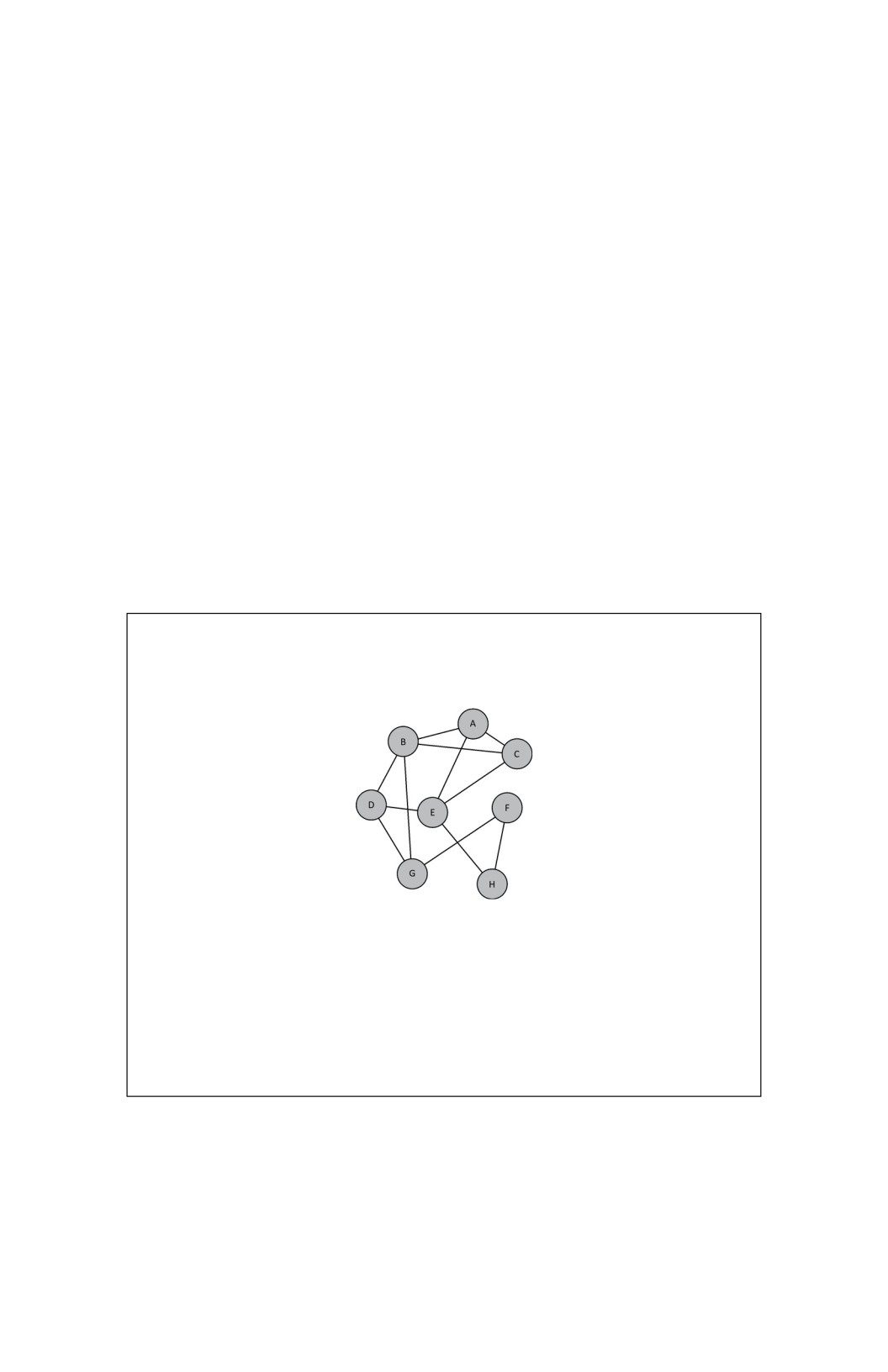
At this point in our discussion, it may be helpful to examine a
classic example of a problem in NP. A Hamiltonian cycle
is a path in a graph that visits all nodes exactly once and
returns to the path’s start. Finding this kind of cycle can be
useful. Consider a delivery truck that needs to make many
stops. A helpful path might be one that leaves the
warehouse, visits all the necessary stops (without repeating
any), and returns to the warehouse. For the example
graph below, we may wish to solve the decision problem of
“Given the graph G = {V, E}, does a Hamiltonian cycle
exist?”
We will discuss the complexity of solving this
problem soon, but for now, we will consider how to verify a
solution to the problem. Suppose that we are given this
problem and a potential solution. How would we verify the
Figure 12.1

correctness of the solution? The “proof” or “certificate” of
this problem could be the ordered list
of vertices in the cycle. We could easily verify this solution
by attempting to traverse the nodes (or vertices) in order
along the graph. If we visit all the vertices and return to
the starting vertex, the verification algorithm could report
“yes.” This would only require work proportional to the
number of nodes, so verifying a solution to the
Hamiltonian cycle problem would have a time complexity
of O(n), where n is the number of nodes in the graph.
This
means that this problem could be easily verified, and by
“easily,”
we mean it could be verified in polynomial time.
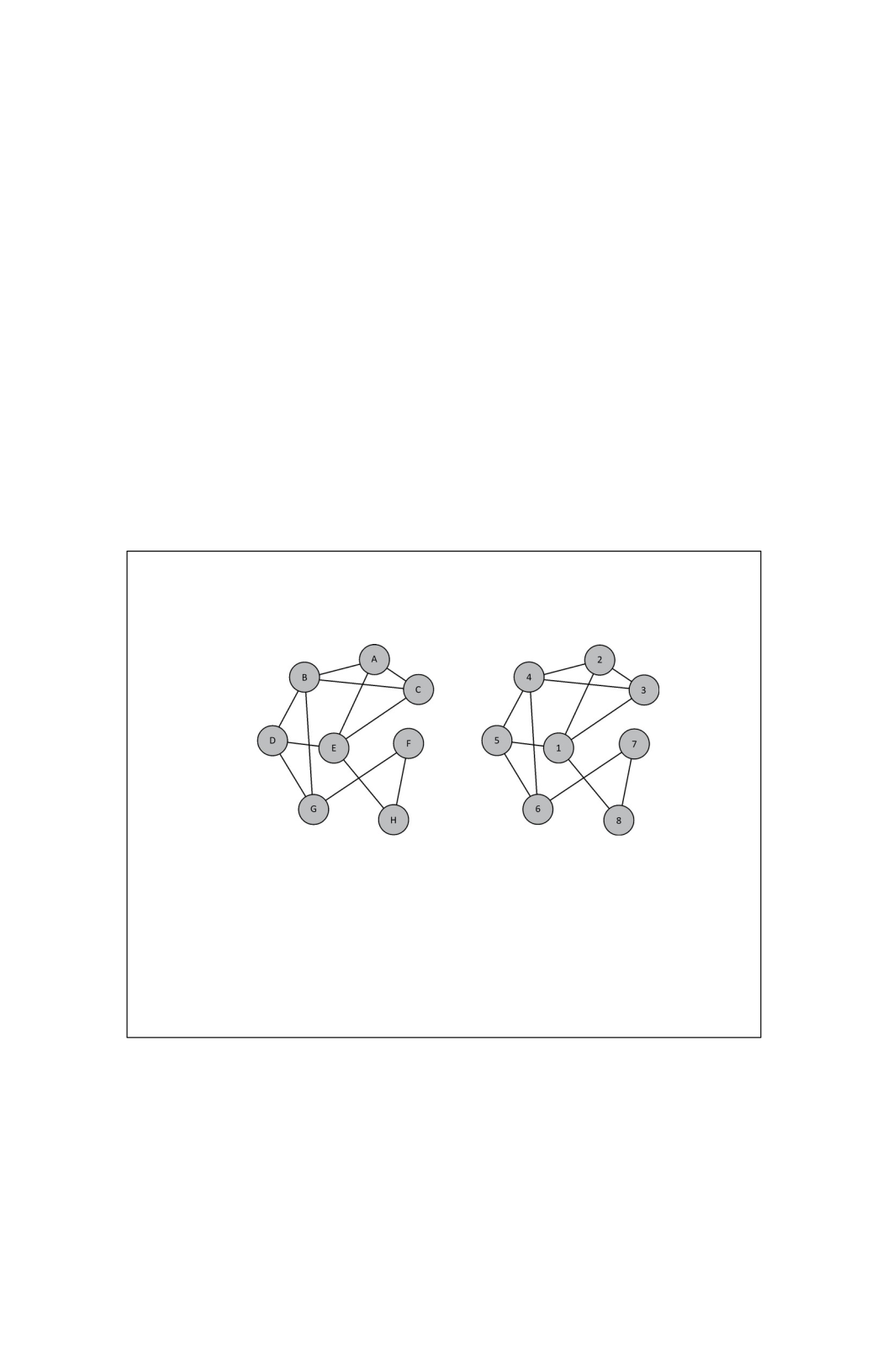
For the above graph, a Hamiltonian cycle would be {E, A,
C, B, D, G, F, H, E}. Note that we must return to the
original position for the path to be a cycle. This is
illustrated below:
The fact that the Hamiltonian cycle problem can be
easily verified may give the (false) impression that it is
also easily solvable. This does not appear to be the
case. One approach to solve it might be to enumerate all
the possible cycles and verify each one. Each cycle would
be some permutation of all the vertices. With n as the
Figure 12.2

number of vertices in the graph, this means that there

would be O(n!) possible orderings to check! This naïve
algorithm is even slower than exponential time O(2n). In
fact, one of the best algorithms known to solve it has a
runtime complexity of O(2nn
2
)—better than O(n!) but still
extremely slow for relatively small n.
Before we move on to the next section, let’s
consider the P complexity class in the context of NP. It
should be clear that any problem in P must also be in NP.
If a problem can be easily solved, it should also be easily
verified. Consider for a moment the opposite situation
where a problem is easy to solve but difficult to verify.
Struggling to verify a solution to a problem might call into
question how easily it was solved. The complexity class P
represents all problems solved in polynomial time, and it is
a subset of the NP class. Now whether it is a “proper
subset” or not of NP is a classic unsolved problem in
computer science theory. A proper subset means that it
cannot be equivalent to the NP class itself. From this
discussion, it may seem as though P and NP are not the
same set, but many brilliant mathematicians and scientists
have attempted to prove or disprove this fact without any
success for decades. Whether P = NP or not remains
unknown. In the next section, we will discuss this further
and highlight just why the P = NP or P ≠ NP question is so
interesting.
Polynomial Time Reductions
In this section, we will introduce the idea of a reduction.
Informally, the term “reduction” refers to a method of
casting one problem instance as an instance of another
problem such that solving the new “reduced” problem also
solves the original. As we explore the next two complexity
classes of NP-hard and NP-complete, we use this powerful
idea of reductions. Using an efficient reduction to

transform one problem into another would serve as a key
to solving a lot of different problems.
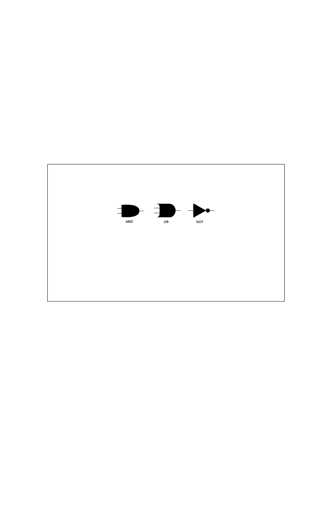
We will briefly consider a classic problem known as
the Circuit-Satisfiability Problem. This is often
abbreviated as CIRCUIT-SAT, but this could also represent
the set of all circuit satisfiability problems (or, specifically,
their instances). Suppose we want to determine if a circuit
composed of logic gates has some assignment to its inputs
that makes the overall circuit output 1. The circuits are
composed of logic gates that take inputs that are either 0
or 1, standing for either low or high voltage. The typical
diagram for these gates is given below:
These gates correspond to their interpretation in
mathematical logic. This means that the AND gate will output
a 1 when both of its inputs are 1. We can compose these
gates into larger circuits. The image below presents an
example of a circuit that uses several of these gates and
takes three inputs, marked X, Y, and Z:
Figure 12.3
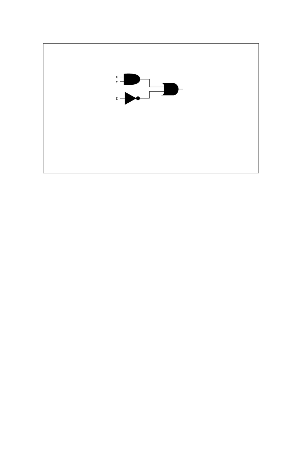
The decision problem for CIRCUIT-SAT would decide
the question of “Given a representation of a circuit composed
of logic gates, does an assignment of zeros and ones to the
inputs exist that makes the overall circuit output 1?” Such
an assignment of inputs is said to satisfy the circuit. One
method of solving this problem would be to try all possible
combinations of 0 and 1 assignments. Given n inputs, this
would be attempting to try O(2n) possibilities. Given a
potential solution, we could verify the assignment satisfies
the circuit by simply simulating the propagation of input
values through the sequence of logic gates. An algorithm for
solving CIRCUIT-SAT problems would be very useful. Let’s look
at why.
Suppose we have another problem we wish to solve:
Given a logical formula, can we provide an assignment to
the logical Boolean variables that satisfies the formula? To
satisfy the formula means to find an assignment of true or
false values to the variables that makes the overall formula
true. This is known as the Boolean satisfiability problem,
and these problem instances are usually referred to as the
set SAT. A logical formula can be composed of variables
and Boolean functions on those variables. These are the
functions AND, OR, and NOT. These are usually written as the
symbols ˄ (AND), ˅ (OR), and ¬ (NOT). Additionally, the
Figure 12.4

formulas use
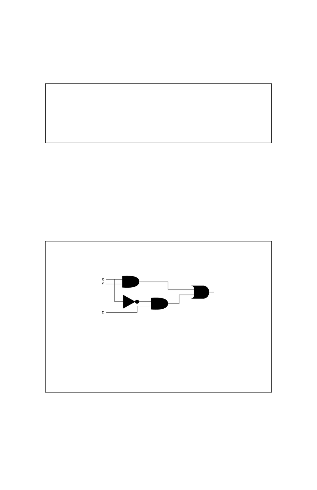
parentheses to make sure there are no ambiguous
connections. An example of a Boolean formula is given
below:
Formulas such as this can be used to model many
problems in computer science. If we had an algorithm that
could solve CIRCUIT-SAT problems, Boolean formula
problems could be solved by first constructing a circuit that
matched the formula and then passing that circuit
representation to the algorithm that decides CIRCUIT-SAT.
The figure below gives a circuit that corresponds to the
Boolean formula given above:
An assignment of 0 or 1 to the inputs of this circuit
would correspond to an assignment of true or false to the
Boolean variables of the formula. While not a formal proof,
hopefully this illustration demonstrates how one instance of
(x ˄ y) ˅ (¬x ˄ z).
Figure 12.5

a problem can be cast into another and a solution to one
can be used to solve the

other. A key point is that this conversion must also be
efficient. For this strategy to be effective, the reduction
from one problem (SAT) to another problem (CIRCUIT-
SAT) must also be efficient. If just doing the reduction was
intractable and difficult, then we would not make any
progress. We will only be interested in reductions that can
be done in polynomial time. For this problem, we could
create a procedure that would parse a string
representation of the formula and generate a parse tree.
From this tree, we could use each branching node to
represent a logic gate, and from this, we could construct a
representation of the circuit. Generating the parse tree
might require O(n
3
) operations (this is an upper bound on
some parsing algorithms), and converting the tree could be
done using a tree traversal costing O(n). This means that
for this case, we could efficiently “reduce” the SAT
problem into an instance of CIRCUIT- SAT.
We will introduce the notation for reducibility here,
as it will be helpful in the following discussions. Remember
that we can also talk about the representations of
problems as being strings in a language. We might say
that SAT, or all the problems in SAT, represents a language
L
1
. The problems in CIRCUIT-SAT represent the language
L
2
. Now to capture the above discussion in this notation,
we would write L1 ≤P L2, using a less than or equal to
symbol with a P subscript. The meaning of L1 ≤P L2 is that
L1 is polynomial-time reducible into an instance of L
2
.
The less than or equal to symbol is used to mean that
problems in L
2
are at least as hard as problems in L
1
. The P
subscript is there to remind us that the reduction must be
doable in polynomial time for this to be a useful reduction.
Let’s provide one more example of a reduction. Another
interesting and well-studied problem in computer science
is the Traveling Salesman Problem or TSP. This
problem tries to solve the practical task of minimizing the
amount of travel between the different cities for a
salesperson before they return home. Another way to cast
the problem might be to ask, “What is the route that

minimizes energy usage for a delivery truck such that it
makes

all its stops and returns to the warehouse?” You may
already be thinking back to our discussion of Hamiltonian
cycles. The TSP is looking for a minimum-cost tour, which
is precisely a Hamiltonian cycle. To consider the decision
version of the TSP, we would take a graph with edge
weights representing the costs of traveling from one
destination to another and a cost threshold k. The decision
problem then asks, “Given the weighted graph G and the
threshold k, does there exist a minimum cost tour with a
cost at most k?” So an instance of the Hamiltonian cycle
problem could be reduced to an instance of the TSP.
Taking an instance of the Hamiltonian cycle problem, we
could construct a new graph with all edge weights set to 0.
This could be done easily in polynomial time by modifying
the representation of the graphic. This new weighted graph
could be passed to an algorithm from solving TSP with k
set to 0. Let’s let the set of all instances of Hamiltonian
cycle problems be HAM-CYCLE. This means that we have
HAM-CYCLE ≤P TSP, and any algorithm that solves
instances of TSP can solve instances of HAM-CYCLE.
The NP-Hard and NP-Complete
Complexity Classes
Reductions serve as a key to solving problems by taking
them from one type of problem and transforming them
into another. We explored two examples of reductions in
the previous section. The SAT problems are reducible to
the CIRCUIT-SAT problems. The HAM-CYCLE problems are
reducible to the TSP problems. Other clever results have
demonstrated that three-coloring a graph is reducible to
the SAT problems. Interestingly, there are algorithms that
can solve any problem in NP by reducing them from other
problem types into an instance of a specific NP problem.
These problems represent the NP-hard complexity class.

More formally, an NP-hard problem is a problem
(language) L, such that for any

problem L′ in NP, L′ ≤P L. In other words, any algorithm for
solving an NP-hard problem could solve any problem in
NP. All four of our
problems—CIRCUIT-SAT, SAT, HAM-CYCLE,
and TSP—are NP-hard.
The Cook–Levin theorem proved
an interesting result showing that SAT is both in NP-hard
(can be used to solve any NP problem) and in NP (easily
verifiable). The class of problems with these characteristics
is known as the NP-complete problems.
Now we revisit the P = NP or P ≠ NP question.
Why is this a big deal? Suppose a problem set (and
algorithm) could be found that was in NP-complete and in
P. This would mean we have an NP-hard problem that can
be easily solved. This result would
mean that any NP problem could be easily solved in O(nk) time.
We would simply reduce any NP problem into an instance
of our special problem and solve it in polynomial time. This
scenario would be the incredible result of a P = NP
reality. The question is still up for debate, and no one
has been able to prove this fact or, more importantly,
find the algorithm. A world in which all difficult problems
could be easily solved would certainly be interesting. For
now, it is unknown whether P = NP or P ≠ NP. Many believe
that P ≠ NP is the more likely scenario, but it has never
been proven.
Approximation Algorithms and
Heuristics
We should discuss the practical matter of how to solve
difficult problems. We have given a somewhat formal
description of NP- Hard and NP-Complete complexity
classes, but let’s reconsider these problems in practical
terms. Suppose we need to solve a SAT problem with 60
variables, and we brute-force search by trying every

combination of Boolean assignments and evaluating them.
The brute-force search requires O(2n) operations. So with
60 variables, the number of combinations is on the order of
2
60
. We call the set of all possible solutions the search
space. If we assume a computer could check 2 billion
of these possible assignment

solutions per second (which is reasonable), we could
expect the calculation to be completed in about 18 years.
The worst-case exponential time complexity for exploring
the search space means that solving these problems
quickly is impossible even for relatively small n (< 100).
We want solutions very quickly and cannot wait 18
years to figure out our best delivery route for this
morning’s deliveries. Delivery companies want to be
efficient to conserve energy. Factories want to maximize
output and keep their machines running. Sometimes a
great approximate solution to an NP- complete
problem can be found quickly. An approximate solution is
not totally correct, but it may satisfy many of the
problem’s requirements. Suppose that we found a SAT
assignment that could satisfy most of our Boolean
formula’s expressions in the previous example; then this
might still be very useful. Many real-world problems can be
modeled by NP-complete problems, so finding good
approximations for them is important work.
Many strategies exist for finding good
approximations. The search for a good approximation can
be framed as an optimization problem. We want to
optimize a current solution’s value toward the optimal
value of a fully correct solution. One approach might be
to randomly try many different solutions and calculate the
value. Each time you find a solution with a better value,
you save it as the current best. You let the algorithm
run for a fixed amount of time. When the time is up,
return the best solution that was found. In general, the
search for a good approximation makes use of heuristics.
Heuristics are strategies or policies that help direct a
search algorithm toward better approximations. The hope
is that the heuristic will help guide the search toward an
optimal solution. Unfortunately, this is not a guarantee.
Algorithms usually act on local information, so any
heuristic might be guiding the search toward a local
optimum while the global optimum is in the other
direction. Developing heuristics for NP-complete

problems is an active field of research. We will look at one
heuristic, the greedy algorithm, and see how it might be
applied to an NP-Hard problem.
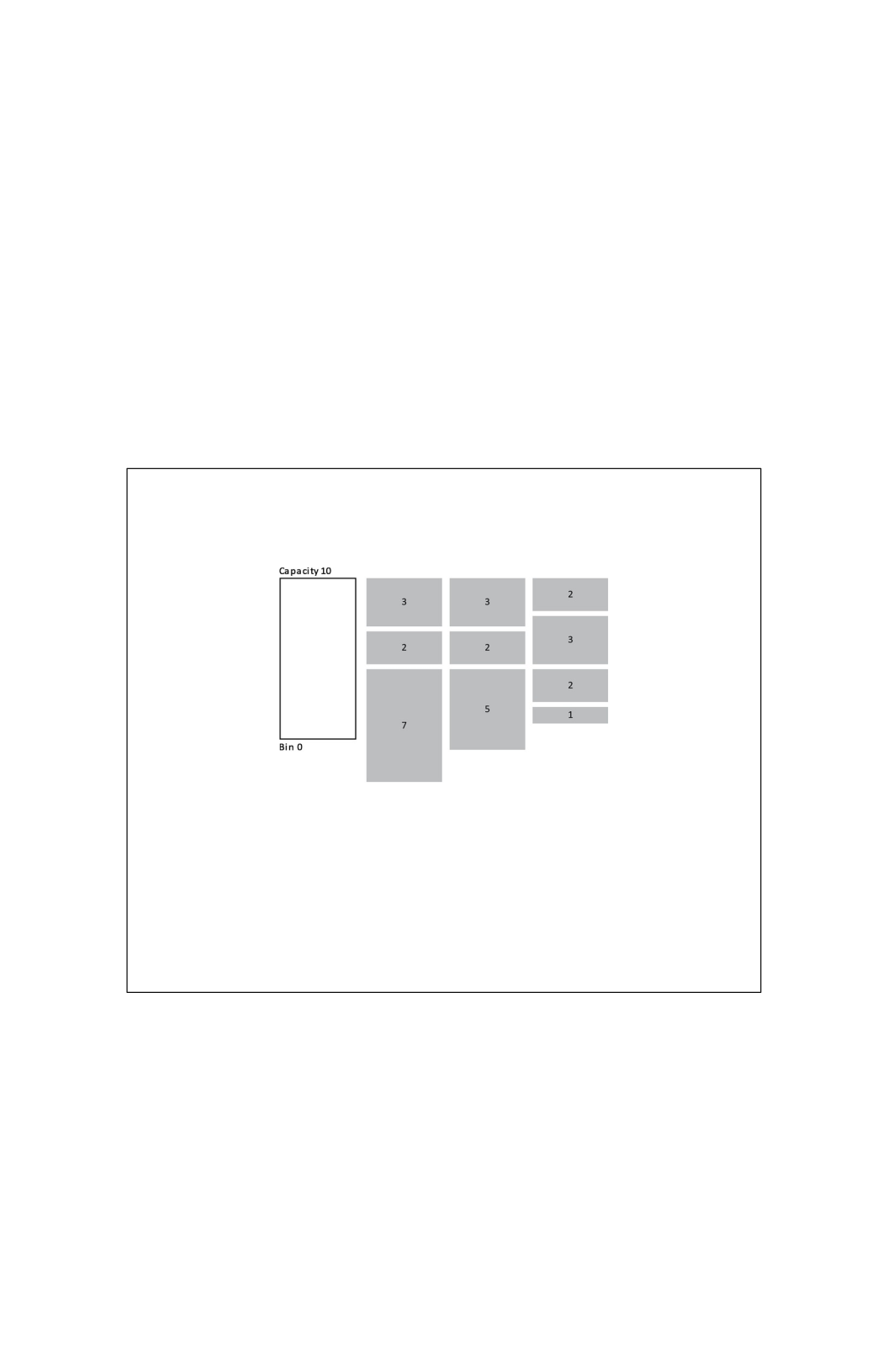
The greedy algorithm uses the heuristic to always
make the choice that maximizes the current value. To
explore this heuristic, we will introduce another NP-hard
problem. The bin packing problem seeks to optimally
pack objects of different sizes into a fixed-size bin. Each
item has a cost associated with it, and the bin has a
capacity threshold where no items may be added that
would push the total cost over the threshold. You can
think of this as the bin getting full of stuff, and nothing
else can be put in it. The example below gives an
illustration of the bin packing problem:
Given the boxes and their sizes, is there a way to
pack all the boxes in the minimum number of bins? It
might seem simple, but to solve this problem optimally, in
general, might require a lot of time. One approach to
finding the optimal number of bins would be to try all
orderings of the items. Attempt to create bins by taking
the items in the ordering and opening a new bin when the
first is full. By trying all possible orderings of the items, the
Figure 12.6

optimal bin number would be found, but this would take
O(n!) time.
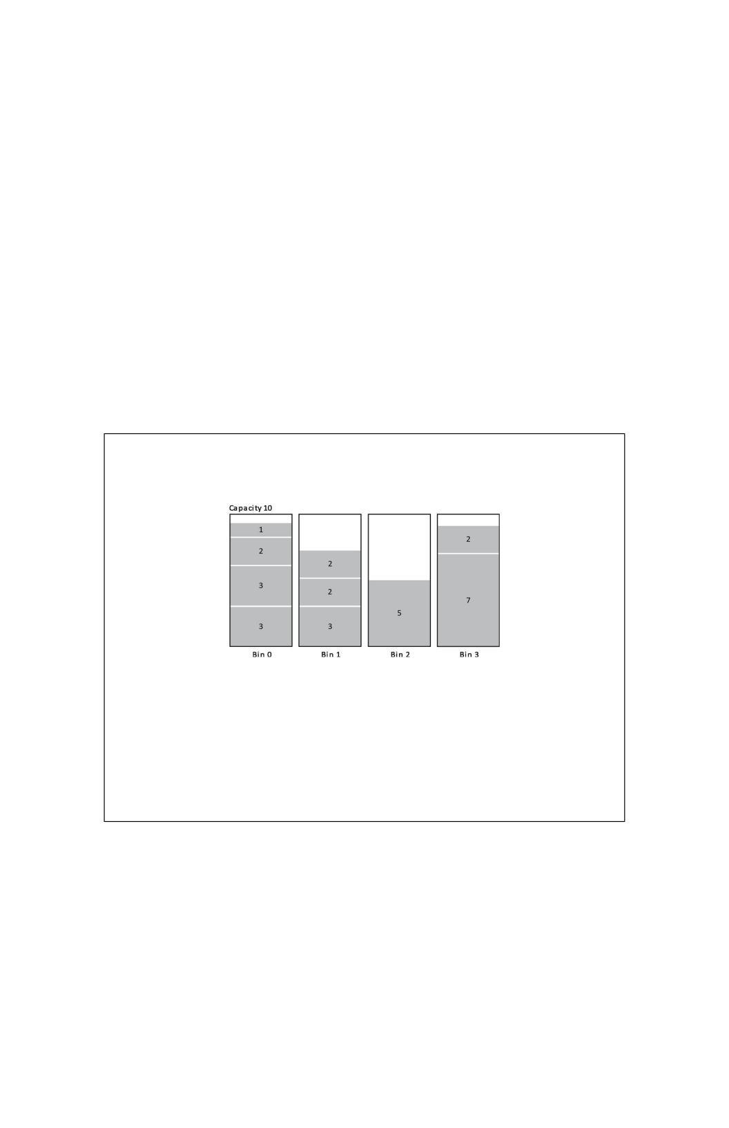
Using the greedy heuristic may help speed up our
search even if the result may be suboptimal. A greedy
algorithm tries to maximize or minimize the current value
associated with a solution. For bin packing, a greedy
strategy would be to always put the current item in the
bin that minimizes the bin’s extra capacity. In other words,
put the item in the bin where it fits the tightest. This is
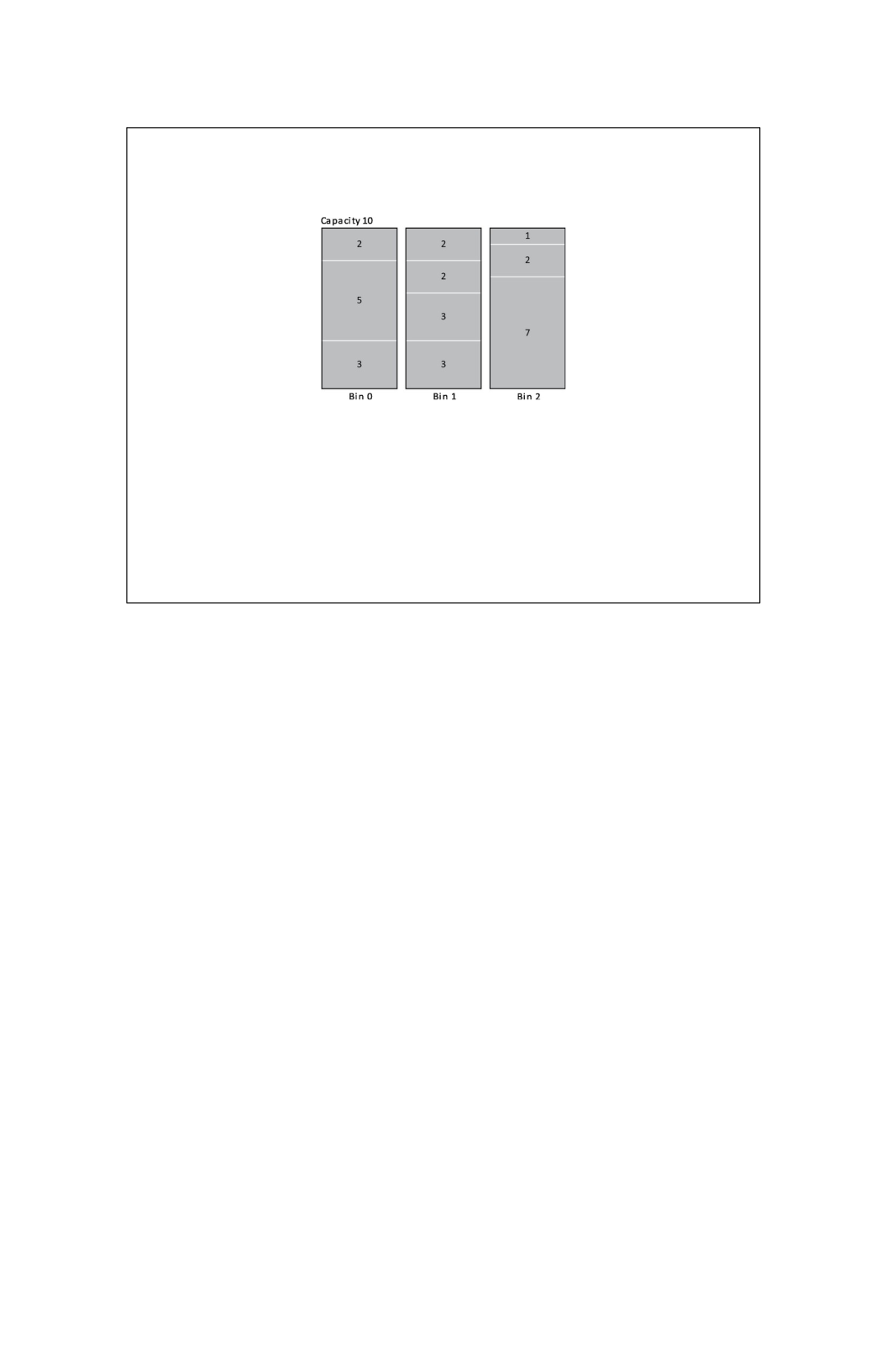
known as the Best Fit algorithm. An example of a Best Fit
solution is presented below for the ordering {3, 3, 2, 3, 1, 2,
2, 5, 7, 2}. This assumes that the items arrive in a fixed order,
and they cannot be reordered. We do get to choose which bin
to place them in though. This is sometimes known as the
“online” version of the bin packing problem.
At each step, the algorithm tries to create the most
tightly packed bin possible. A clever algorithm for Best Fit
achieves an O(n log n) time complexity by querying bins
by their remaining capacity in a balanced binary search
tree. This algorithm is extremely fast compared to the
brute-force method, but it is not optimal. Below is an
optimal solution:
Figure 12.7
Depending on whether the items can be reordered
or not, we may have the opportunity to first sort the items
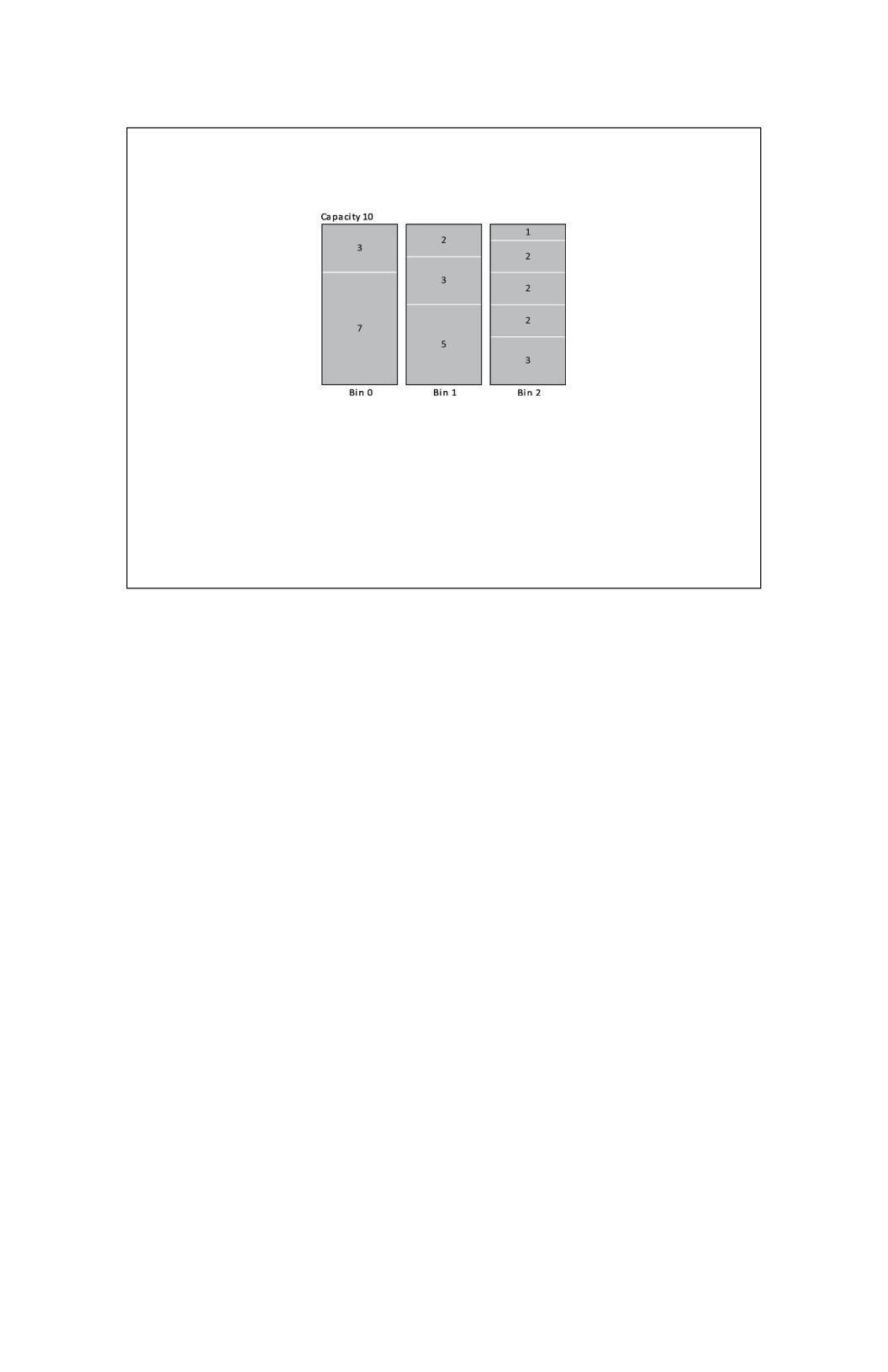
before applying Best Fit. Another good greedy algorithm
for bin packing first sorts the items into descending order
and then applies the Best Fit algorithm. This is known as
Best Fit Decreasing. The figure below shows the result of
applying Best Fit Decreasing to our block problem. This
strategy does yield an optimal solution in this case. This
algorithm would also have an O(n log n) time complexity.
These algorithms show the value of using a heuristic to
discover a good approximate solution to a very difficult
problem in a reasonable amount of time.
Figure 12.8
Bin packing provides insight into another feature of
NP- complete and NP-hard problems. The decision
version of the bin packing problem asks, “Given the n
items and their sizes, can all items be packed into k or
fewer bins?” This decision problem turns out to be NP-
Complete. Given a potential solution and the number of
bins, we can easily verify the number of bins used and the
excess capacity in O(n) time. This fact confirms that the
problem is in NP. Even with a target number of bins given,
we would have to try overwhelmingly many configurations
to ultimately determine if all the items would fit into the k
bins. Now we may also be interested in determining the
optimal number of bins. This decision problem might be
asked as “Given the n items and their sizes, does the
minimum packing require at most k bins?” Consider how
we might verify that the optimal configuration was found.
This means that we were given a solution and told it is
optimal. We would now need to verify it. We could easily
verify if the solution fits into the given number of bins. On
the other hand, verifying that the number of bins for this
solution is optimal would require considering all the
possible solutions and checking that no other solution
Figure 12.9

exists with a smaller number of bins. This means that the
optimization version

of this problem is not in NP. Therefore, the optimization
problem is only NP-hard and not NP-complete. This
pattern is common with NP-complete problems. If the
decision version of a problem is NP- complete, its
optimization version is usually only in NP-hard.
In our discussion of hard problems, we need to first define
some sets of problems and their properties. First, let’s
think about a problem that needs to be solved by a
computer. A sorting problem, for example, provides an
ordered list of numbers and asks that they be sorted.
Solving this problem would provide the same numbers
reordered such that they are all in increasing order. We
know that there exist sorting algorithms that can solve this
problem in O(n
2
) and even O(n log n) time. Problems such
as these belong to the P complexity class. P represents
the set of all problems for which there exists a polynomial
time algorithm to solve them. This means that an
algorithm exists for solving these problems with a time
scaling function bounded by O(nk) for some constant k.
Strictly speaking, P is reserved only for decision
problems, a problem with only a yes or no solution. This is
not a serious limitation from our perspective. Many of the
problems we have seen in this book can be easily
reformulated as decision problems of equal difficulty.
Suppose there is an algorithm, let’s identify it as

A, that solves instances of a decision problem in P. If A
can solve any instance of the problem in polynomial time,
then we say that A decides that set of problem instances.
For any input that is an instance of our problem, A will
report 1. In this case, we say A accepts the input. If any
input is not an instance of that decision problem, A will report
0. In this case, we say A rejects that input.
By framing our algorithms as decision problems,
we can rely on some concepts from formal language theory.
From this framework, we think about encoding our inputs as
strings of 0 and 1 symbols. We should know numbers can
be encoded in binary, but other types of data, such as
images and symbol data, can also be so encoded. At some
level, all their data are stored in binary on your phone or
computer. We can use 0 and 1 as symbols to construct the
strings of our binary language. In the formal language model,
A acts as a language recognizer. If the input string is part
of our specific language of problem instances, A will
accept it as part of the language. If an input string is not
part of the problem set of instances, A will reject it as we
discussed in the previous paragraph. This is one of the
formalizations that have been used to reason about
problems in theoretical computer science. We will not
explore formal languages any further here, but this model is
equivalent to the practical problem-solving we have explored
in this textbook. The language model also closely relates to
the simplest theoretical model of computing, the Turing
Machine.
The concept of determinism is another important
idea to introduce in our discussion of the complexity class
P. The P class is described as the class of deterministic
polynomial time problems. This requires a bit of subtlety to
describe accurately. For now, we will just say that the
algorithms for solving problems in P function
deterministically in a step-by-step fashion. This could be
interpreted as meaning that the algorithms can only take
one step at a time in their execution. This definition will
make more sense as we discuss the next complexity

class, NP, or the class of nondeterministic polynomial time
problems.

The NP Complexity Class
We think of problems in P as being easy because
“efficient” algorithms exist to solve them. By efficient, we
mean having polynomial time complexity, O(nk). The NP
complexity class introduces some problems that can be
considered fairly hard. NP stands for nondeterministic
polynomial time complexity. The NP class of problems
introduces the idea of solution verification. If you were
given the solution for an algorithm, could you verify that it
was correct? Think about how you might verify that a list of
numbers is sorted. How could you verify that 7! = 5040?
I’m sure you can think of several ways to easily check
these answers in a short amount of time. Again, we will
focus on decision problems, but decision versions of all
problems can be constructed such that we do not lose
generality in this discussion. For a problem to be in NP,
there must exist an algorithm A that verifies instances of
the problem by checking a “proof” or “certificate.” You
may think of the certificate as a solution to the problem
that must be verified in polynomial time.
NP leaves the question of whether a problem can
be solved quickly and considers whether the solution could
be verified quickly. The nondeterministic part refers to
the idea of ignoring how quickly the problem could be
solved. We mentioned that a deterministic algorithm could
take only one step at a time. We could think of a
nondeterministic algorithm as one that could take many
steps “at the same time.” One interpretation of this might
be considering all options simultaneously. The main
takeaway is that a correct solution must be verifiable in
polynomial time for the problem to be a member of NP.
An Example of an NP Problem:
Hamiltonian Cycle
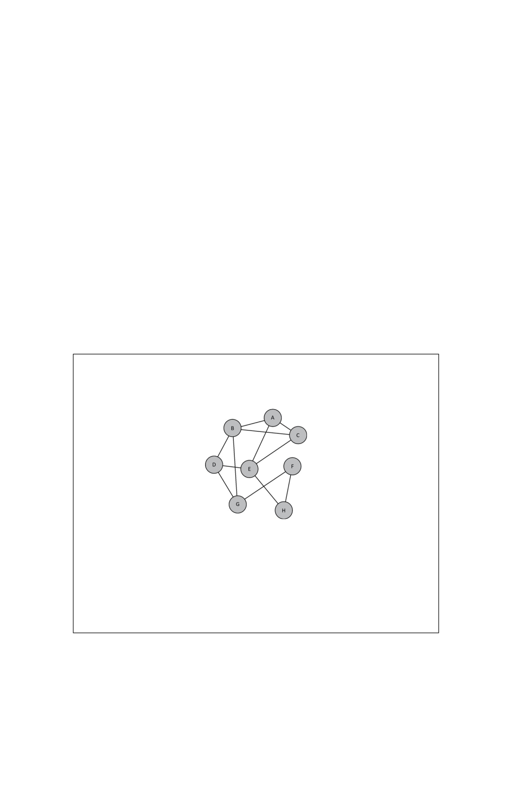
At this point in our discussion, it may be helpful to examine a
classic example of a problem in NP. A Hamiltonian cycle
is a path in a graph that visits all nodes exactly once and
returns to the path’s start. Finding this kind of cycle can be
useful. Consider a delivery truck that needs to make many
stops. A helpful path might be one that leaves the
warehouse, visits all the necessary stops (without repeating
any), and returns to the warehouse. For the example
graph below, we may wish to solve the decision problem of
“Given the graph G = {V, E}, does a Hamiltonian cycle
exist?”
We will discuss the complexity of solving this
problem soon, but for now, we will consider how to verify a
solution to the problem. Suppose that we are given this
problem and a potential solution. How would we verify the
Figure 12.1

correctness of the solution? The “proof” or “certificate” of
this problem could be the ordered list
of vertices in the cycle. We could easily verify this solution
by attempting to traverse the nodes (or vertices) in order
along the graph. If we visit all the vertices and return to
the starting vertex, the verification algorithm could report
“yes.” This would only require work proportional to the
number of nodes, so verifying a solution to the
Hamiltonian cycle problem would have a time complexity
of O(n), where n is the number of nodes in the graph.
This
means that this problem could be easily verified, and by
“easily,”
we mean it could be verified in polynomial time.
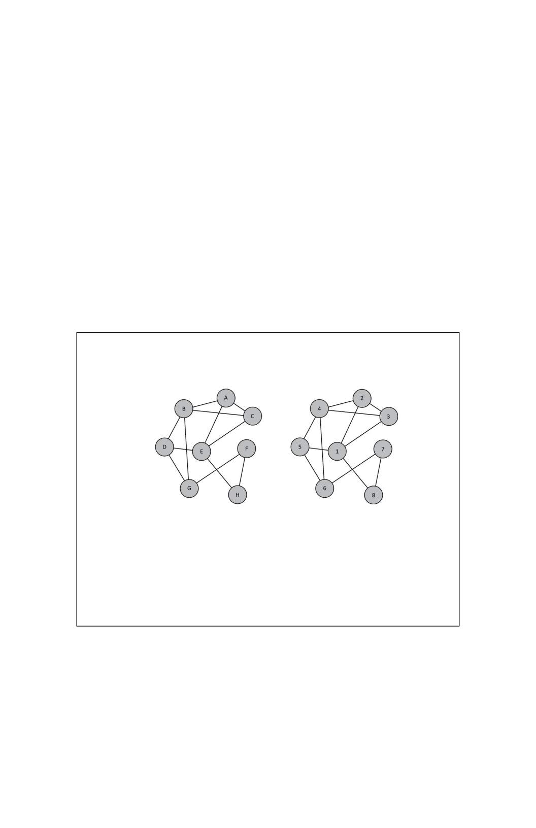
For the above graph, a Hamiltonian cycle would be {E, A,
C, B, D, G, F, H, E}. Note that we must return to the
original position for the path to be a cycle. This is
illustrated below:
The fact that the Hamiltonian cycle problem can be
easily verified may give the (false) impression that it is
also easily solvable. This does not appear to be the
case. One approach to solve it might be to enumerate all
the possible cycles and verify each one. Each cycle would
be some permutation of all the vertices. With n as the
Figure 12.2

number of vertices in the graph, this means that there

would be O(n!) possible orderings to check! This naïve
algorithm is even slower than exponential time O(2n). In
fact, one of the best algorithms known to solve it has a
runtime complexity of O(2nn
2
)—better than O(n!) but still
extremely slow for relatively small n.
Before we move on to the next section, let’s
consider the P complexity class in the context of NP. It
should be clear that any problem in P must also be in NP.
If a problem can be easily solved, it should also be easily
verified. Consider for a moment the opposite situation
where a problem is easy to solve but difficult to verify.
Struggling to verify a solution to a problem might call into
question how easily it was solved. The complexity class P
represents all problems solved in polynomial time, and it is
a subset of the NP class. Now whether it is a “proper
subset” or not of NP is a classic unsolved problem in
computer science theory. A proper subset means that it
cannot be equivalent to the NP class itself. From this
discussion, it may seem as though P and NP are not the
same set, but many brilliant mathematicians and scientists
have attempted to prove or disprove this fact without any
success for decades. Whether P = NP or not remains
unknown. In the next section, we will discuss this further
and highlight just why the P = NP or P ≠ NP question is so
interesting.
Polynomial Time Reductions
In this section, we will introduce the idea of a reduction.
Informally, the term “reduction” refers to a method of
casting one problem instance as an instance of another
problem such that solving the new “reduced” problem also
solves the original. As we explore the next two complexity
classes of NP-hard and NP-complete, we use this powerful
idea of reductions. Using an efficient reduction to

transform one problem into another would serve as a key
to solving a lot of different problems.

We will briefly consider a classic problem known as the Circuit-
Satisfiability Problem. This is often abbreviated as CIRCUIT-SAT, but
this could also represent the set of all circuit satisfiability problems (or,
specifically, their instances). Suppose we want to determine if a circuit
composed of logic gates has some assignment to its inputs that makes
the overall circuit output
The
Halting
Problem
Before we end the chapter, we should discuss one of the
classic problems in computer science, the halting
problem. The halting problem illustrates the existence of
“unsolvable” problems. Alan Turing proved the existence
of a particular undecidable problem. The halting problem
can be defined as asking the question “Given a
representation of a computer program and the program
input, will the program halt for that given input or run
forever?” Turing’s argument proposed the existence of a
program (an algorithm running on a machine) that could
detect if another program would halt given a specific input.
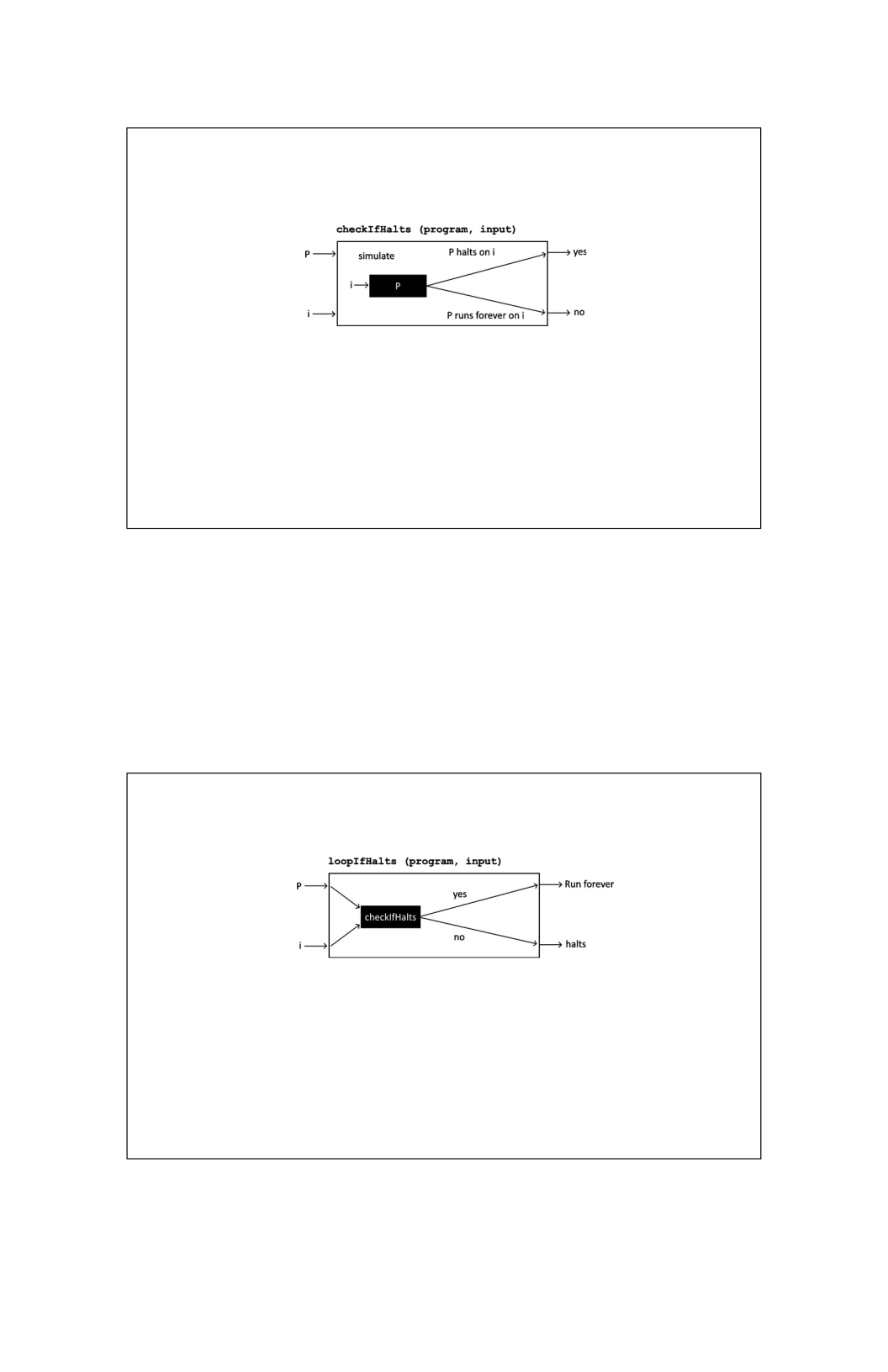
Let’s just informally say we have a function like
checkIfHalts(program, input). If the input program
would halt, meaning complete successfully, on the given
input, then checkIfHalts would report yes. If the program
would run forever given the input, checkIfHalts would
report no. This would be an algorithm that decides the
halting problem. Running this hypothetical algorithm on a
machine would allow a scheme for deciding if a program
would halt. The program checkIfHalts would simulate the
program P with the given input and decide if P halts on the
input. This machine is presented in a diagram below:
The interesting part of the argument suggests that
our program runs with its own representation presented as
the input. Let’s construct another machine using
checkIfHalts that will run forever if the program halts
given an input but will halt if the program runs forever (as
verified by checkIfHalts). Below is a diagram of this
machine. We will call it loopIfHalts.
Now we construct one final machine as follows.
This machine will take as input the representation of a
Figure 12.10
Figure 12.11

program and
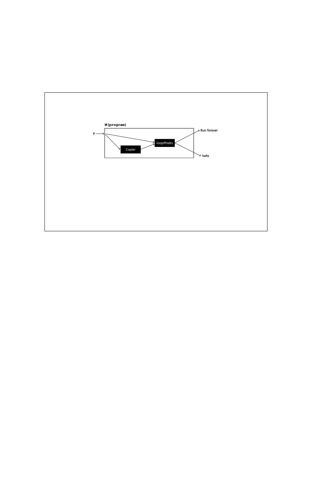
try to determine if that program would halt when given a
representation of itself as input. This is done by copying
the program and using the copy as input. This machine is
presented below. We will just call this M(program).
Now suppose that we run M with a representation of M
as
the input. We can think of this as calling M(M). If the
program M should halt given M as the input, then M(M)
should run forever. However, this is exactly what we did.
We passed M into M, and if it runs forever, then M(M)
should halt. This leads to a contradiction. We have a
paradox where M should both run forever and halt. Since
we arrived at a contradiction and all these algorithms
(loopIfHalts and M) are derived from our hypothetical
checkIfHalts program, these facts indicate that such a
program cannot exist. This means that the halting problem
is undecidable. This proof was discovered by Alan Turing
and published in 1936. It provided some of the first
evidence of problems that were literally unsolvable. Now
that’s a hard problem! In our discussion of hard problems,
we need to first define some sets of problems and their
properties. First, let’s think about a problem that needs to
be solved by a computer. A sorting problem, for example,
Figure 12.12

provides an ordered list of numbers and asks that they be
sorted. Solving this problem would provide the same
numbers reordered such that they are all in increasing
order. We know that there exist sorting algorithms that can
solve this problem in O(n
2
) and even O(n log n) time.
Problems such as these belong to the P complexity class.
P represents the set of all problems for which there exists
a polynomial time algorithm to solve them. This means
that an algorithm exists for solving these problems with a
time scaling function bounded by O(nk) for some constant
k.
Strictly speaking, P is reserved only for decision
problems, a problem with only a yes or no solution. This is
not a serious limitation from our perspective. Many of the
problems we have seen in this book can be easily
reformulated as decision problems of equal difficulty.
Suppose there is an algorithm, let’s identify it as

A, that solves instances of a decision problem in P. If A
can solve any instance of the problem in polynomial time,
then we say that A decides that set of problem instances.
For any input that is an instance of our problem, A will
report 1. In this case, we say A accepts the input. If any
input is not an instance of that decision problem, A will report
0. In this case, we say A rejects that input.
By framing our algorithms as decision problems,
we can rely on some concepts from formal language theory.
From this framework, we think about encoding our inputs as
strings of 0 and 1 symbols. We should know numbers can
be encoded in binary, but other types of data, such as
images and symbol data, can also be so encoded. At some
level, all their data are stored in binary on your phone or
computer. We can use 0 and 1 as symbols to construct the
strings of our binary language. In the formal language model,
A acts as a language recognizer. If the input string is part
of our specific language of problem instances, A will
accept it as part of the language. If an input string is not
part of the problem set of instances, A will reject it as we
discussed in the previous paragraph. This is one of the
formalizations that have been used to reason about
problems in theoretical computer science. We will not
explore formal languages any further here, but this model is
equivalent to the practical problem-solving we have explored
in this textbook. The language model also closely relates to
the simplest theoretical model of computing, the Turing
Machine.
The concept of determinism is another important
idea to introduce in our discussion of the complexity class
P. The P class is described as the class of deterministic
polynomial time problems. This requires a bit of subtlety to
describe accurately. For now, we will just say that the
algorithms for solving problems in P function
deterministically in a step-by-step fashion. This could be
interpreted as meaning that the algorithms can only take
one step at a time in their execution. This definition will
make more sense as we discuss the next complexity

class, NP, or the class of nondeterministic polynomial time
problems.

The NP Complexity Class
We think of problems in P as being easy because
“efficient” algorithms exist to solve them. By efficient, we
mean having polynomial time complexity, O(nk). The NP
complexity class introduces some problems that can be
considered fairly hard. NP stands for nondeterministic
polynomial time complexity. The NP class of problems
introduces the idea of solution verification. If you were
given the solution for an algorithm, could you verify that it
was correct? Think about how you might verify that a list of
numbers is sorted. How could you verify that 7! = 5040?
I’m sure you can think of several ways to easily check
these answers in a short amount of time. Again, we will
focus on decision problems, but decision versions of all
problems can be constructed such that we do not lose
generality in this discussion. For a problem to be in NP,
there must exist an algorithm A that verifies instances of
the problem by checking a “proof” or “certificate.” You
may think of the certificate as a solution to the problem
that must be verified in polynomial time.
NP leaves the question of whether a problem can
be solved quickly and considers whether the solution could
be verified quickly. The nondeterministic part refers to
the idea of ignoring how quickly the problem could be
solved. We mentioned that a deterministic algorithm could
take only one step at a time. We could think of a
nondeterministic algorithm as one that could take many
steps “at the same time.” One interpretation of this might
be considering all options simultaneously. The main
takeaway is that a correct solution must be verifiable in
polynomial time for the problem to be a member of NP.
An Example of an NP Problem:
Hamiltonian Cycle
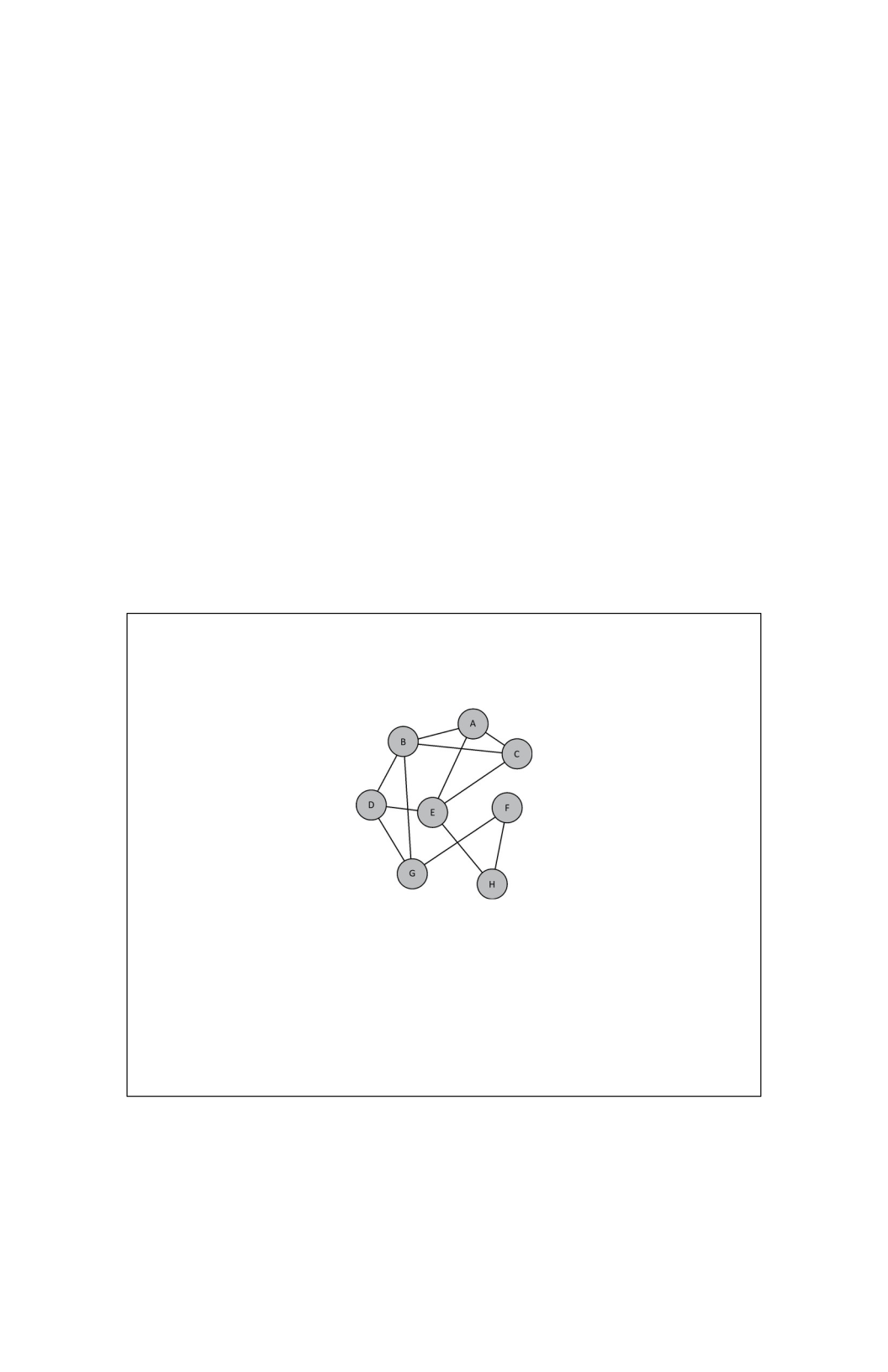
At this point in our discussion, it may be helpful to examine a
classic example of a problem in NP. A Hamiltonian cycle
is a path in a graph that visits all nodes exactly once and
returns to the path’s start. Finding this kind of cycle can be
useful. Consider a delivery truck that needs to make many
stops. A helpful path might be one that leaves the
warehouse, visits all the necessary stops (without repeating
any), and returns to the warehouse. For the example
graph below, we may wish to solve the decision problem of
“Given the graph G = {V, E}, does a Hamiltonian cycle
exist?”
We will discuss the complexity of solving this
problem soon, but for now, we will consider how to verify a
solution to the problem. Suppose that we are given this
problem and a potential solution. How would we verify the
Figure 12.1

correctness of the solution? The “proof” or “certificate” of
this problem could be the ordered list
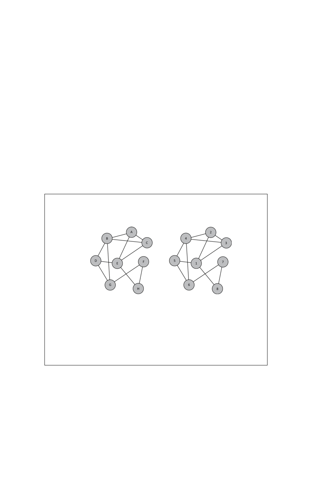
of vertices in the cycle. We could easily verify this solution
by attempting to traverse the nodes (or vertices) in order
along the graph. If we visit all the vertices and return to
the starting vertex, the verification algorithm could report
“yes.” This would only require work proportional to the
number of nodes, so verifying a solution to the
Hamiltonian cycle problem would have a time complexity
of O(n), where n is the number of nodes in the graph.
This
means that this problem could be easily verified, and by
“easily,”
we mean it could be verified in polynomial time.
For the above graph, a Hamiltonian cycle would be {E, A,
C, B, D, G, F, H, E}. Note that we must return to the
original position for the path to be a cycle. This is
illustrated below:
The fact that the Hamiltonian cycle problem can be
easily verified may give the (false) impression that it is
also easily solvable. This does not appear to be the
case. One approach to solve it might be to enumerate all
the possible cycles and verify each one. Each cycle would
be some permutation of all the vertices. With n as the
Figure 12.2

number of vertices in the graph, this means that there

would be O(n!) possible orderings to check! This naïve
algorithm is even slower than exponential time O(2n). In
fact, one of the best algorithms known to solve it has a
runtime complexity of O(2nn
2
)—better than O(n!) but still
extremely slow for relatively small n.
Before we move on to the next section, let’s
consider the P complexity class in the context of NP. It
should be clear that any problem in P must also be in NP.
If a problem can be easily solved, it should also be easily
verified. Consider for a moment the opposite situation
where a problem is easy to solve but difficult to verify.
Struggling to verify a solution to a problem might call into
question how easily it was solved. The complexity class P
represents all problems solved in polynomial time, and it is
a subset of the NP class. Now whether it is a “proper
subset” or not of NP is a classic unsolved problem in
computer science theory. A proper subset means that it
cannot be equivalent to the NP class itself. From this
discussion, it may seem as though P and NP are not the
same set, but many brilliant mathematicians and scientists
have attempted to prove or disprove this fact without any
success for decades. Whether P = NP or not remains
unknown. In the next section, we will discuss this further
and highlight just why the P = NP or P ≠ NP question is so
interesting.
As with other graph properties and algorithms,
MSTs have numerous applications in the natural world. The
canonical example is that of a network broadcast. Imagine
computers as nodes and the network connections
between them as edges. In computer networking, we often
want to be able to broadcast a message to all nodes on the
network (or, put simply, ensure that all nodes receive a
particular message). The MST represents the lowest-cost
means of transmitting such a message. Note that this is
not the fastest means of transmission. That would indeed
be a tree created by running a single-source shortest-path
algorithm like Dijkstra’s.
As with single-source shortest path, MSTs can be

produced via numerous algorithms. The only one we
address here is Prim’s. We do so due to its similarity with
Dijkstra’s. Dijkstra’s produced shortest paths by comparing
a known distance against the sum of the cumulative
distance to the predecessor plus the newly considered edge
(see line 11 in the pseudocode). This comparison can be
made because the distance for a node denotes the
shortest path we have considered so far. Prim’s algorithm
changes the meaning of the distance value as well as
the comparison on line
11. Rather than representing the cumulative distance as we
did for shortest path, distance now represents the cost to
add that node into the MST. The final change is simple: if we
remove n.Dist from both lines 11 and 12, then we now
find the MST rather than a shortest-path tree.
Everyone in life faces hard problems. Figuring out what to
do with your life or career can be hard. You may find it
hard to choose between two delicious menu items. These
problems, while “hard” in their own way, are not the kinds
of hard problems we will be exploring in this chapter. In
this chapter, we will introduce some
of the key ideas that
support the theory of computation, the theoretical
foundation of computer science. The discovery of these

concepts is rather recent in the history of science and
mathematics, but these concepts provide some fascinating
insight into how humanity may attempt to solve the most
difficult problems.
In the following sections, we will introduce the most
discussed complexity classes in theoretical computer
science. These are the complexity classes of P, NP, NP-
complete, and NP- hard. These classes highlight many
interesting and important results in computer science. We
will explore what makes problems “easy” or “hard” in a
theoretical sense. We will then explore some concepts for
tackling these hard problems using approximations and
heuristics. Finally, we will end the chapter with a
discussion of an “impossible” problem, the halting
problem, and what this means for computability.
Polynomial Time Reductions
In this section, we will introduce the idea of a reduction.
Informally, the term “reduction” refers to a method of
casting one problem instance as an instance of another
problem such that solving the new “reduced” problem also
solves the original. As we explore the next two complexity
classes of NP-hard and NP-complete, we use this powerful
idea of reductions. Using an efficient reduction to
transform one problem into another would serve as a key
to solving a lot of different problems.

We will briefly consider a classic problem known as the Circuit-
Satisfiability Problem. This is often abbreviated as CIRCUIT-SAT, but this
could also represent the set of all circuit satisfiability problems (or, specifically,
their instances). Suppose we want to determine if a circuit composed of logic
gates has some assignment to its inputs that makes the overall circuit output

