


Table of Contents
A8.9.5 Identify an Example of a Variable Measured at the Scale/Normally Distributed Level for
Which There Is a Statistically Significant Overall Difference (F) Between the Three Marital
Status Groups. Complete the analysis and interpret the results. Do appropriate post hoc tests......3
A8.9.6 Use the Kruskal–Wallis Test, With Mann‒Whitney Post Hoc Follow-Up Tests If Needed,
to Run the Same Problem as 9.1. Compare the results....................................................................6
A8.9.7 Do Students’ Heights Differ Depending on Academic Track and Marital Status, and Do
Academic Track and Marital Status Interact? Run the Appropriate Analysis and Interpret the
Results..............................................................................................................................................7
A8.9.8 Do Academic Track and Having Children Interact and Does Either Seem to Affect
Current GPA?................................................................................................................................10
References......................................................................................................................................14
1

BUSI 820 – A8 QUANTITATIVE ANALYSIS
A8.9.5 Identify an Example of a Variable Measured at the Scale/Normally Distributed
Level for Which There Is a Statistically Significant Overall Difference (F) Between the
Three Marital Status Groups. Complete the analysis and interpret the results. Do
appropriate post hoc tests.
The variable is hours of study per week. Table 1 provides descriptive statistics for the
three marital status groups on the dependent variable (hours of study per week).
Table 2 provides the Levene's test to check the assumption that the variances of the three
marital status groups are equal for each of the dependent variables. For ANOVA, we are
interested in the test based on means. The Levene's test is not significant (p=0.072). Thus, the
assumption is not violated.
Table 3 is the key table because it shows whether the overall F for the ANOVA
were statistically significant. Note that the three marital status groups differ on hours of study per
week. F(2, 46)=5.861, p=0.005.
Table 1
Descriptives
Table 2
Tests of Homogeneity of Variances
2
10/13/2023

BUSI 820 – A8 QUANTITATIVE ANALYSIS
Table 3
ANOVA
Table 4
ANOVA Effect Sizes
Because the Levene’s test was not statistically significant, the appropriate post hoc test is
Tukey Honestly Significant Difference (HSD) test. The Tukey HSD test is a single-step method
for making multiple comparisons. It is designed to accommodate varying group sizes and relies
3
10/13/2023

BUSI 820 – A8 QUANTITATIVE ANALYSIS
on assumptions of independence among factor levels, consistent variance, and normality. This
test can be applied directly to the raw data or utilized in conjunction with an ANOVA (as a post-
hoc analysis) to identify statistically significant differences in means (Hitka et al., 2017).
Table 5 shows the Tukey HSD test for hours of study per week that you would use if the
three group sizes (n = 20, 18, 11) had been similar. For hours of study per week, this Tukey table
indicates that there are statistically significant differences between the hours of study per week
for those who are single vs married (mean difference = -6.556), single vs divorced (mean
difference = -8.591). There is not a significant difference between hours of study per week for
those who are married vs. divorced.
Table 6, the Homogeneous Subsets table, shows an adjusted Tukey that is appropriate
when group sizes are not similar, as in this case. Note that there is not a statistically significant
difference (p=0.052) between hours of study per week for those who are single vs. married and
for those who are married vs. divorced (p=0.737) By examining the two subset boxes, we can see
that the single group (M = 11.50) is different from the divorced group (M = 20.09) because these
two means do not appear in the same subset.
Table 5
Multiple Comparisons
4
10/13/2023

BUSI 820 – A8 QUANTITATIVE ANALYSIS
Table 6
Hours of Study per Week
A8.9.6 Use the Kruskal–Wallis Test, With Mann‒Whitney Post Hoc Follow-Up Tests If
Needed, to Run the Same Problem as 9.1. Compare the results.
Table 7 provides Mean Ranks for the dependent variable (hours of study per week). In
this case, the Kruskal-Wallis (K-W) test will compare the mean ranks for the three marital status
groups. Table 8 shows whether there is an overall difference among the three groups. Notice that
the p (Asymp. Sig.) value for hours of study per week is 0.155, which is different from the output
5
10/13/2023

BUSI 820 – A8 QUANTITATIVE ANALYSIS
using the one-way ANOVA. Because the K-W test shows that there is not a statistically
significant difference in hours of study per week among the three martial groups, post hoc
follow-up test is not needed.
Table 7
Ranks
Table 8
Test Statistics
A8.9.7 Do Students’ Heights Differ Depending on Academic Track and Marital Status, and
Do Academic Track and Marital Status Interact? Run the Appropriate Analysis and
Interpret the Results.
The 2-way ANOVA was used to answer the question. Students’ heights was used as
dependent variable. Academic track and marital status were used as 2 factors.
6
10/13/2023

BUSI 820 – A8 QUANTITATIVE ANALYSIS
Table 9 shows that 49 participants (21 in fast track and 28 in regular track) are included
in the analysis because they had data on all of the three variables. Table 10 shows the cell and
marginal (total) means; both are very important for interpreting the ANOVA table and
explaining the results of the test for the interaction.
Table 11, the ANOVA table, called Tests of Between-subjects Effects, is the key table.
The interaction F(marital*acadtrac) which, in this case, is statistically significant, F (2,43) =
4.145, p = 0.023. Because the interaction was significant, we need to be cautious about the
interpretation of the main effects because they could be misleading.
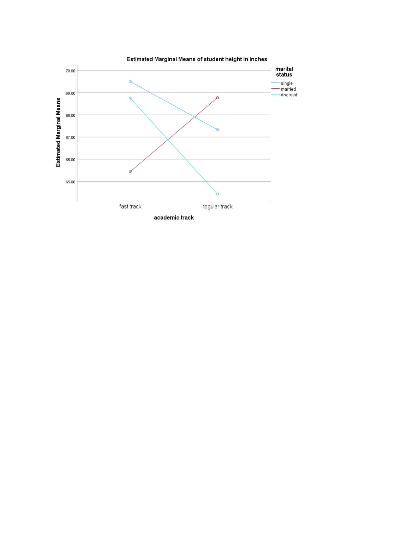
The profile plots may be helpful in visualizing the interaction, but we should not discuss
statistically nonsignificant differences because the plots may be misleading (Morgan et al.,
2020). Next, we examine the main effects of marital status and of academic track. Note that both
are not statistically significant (p=0.388 and p=0.359 respectively). This means that there is not
statistically significant difference in students’ heights between martial status groups, and
between academic track groups.
In Figure 1, the profile plots of cell means, help us to visualize the nature of
a significant interaction when one exists. When the lines on the profile plot are parallel, there is
not a significant interaction.
Table 9
Between-Subjects Factors
7
10/13/2023

BUSI 820 – A8 QUANTITATIVE ANALYSIS
Table 10
Descriptive Statistics
Table 11
Tests of Between-Subjects Effects
Figure 1
Estimated Marginal Means of Student Height in Inches
8
10/13/2023
BUSI 820 – A8 QUANTITATIVE ANALYSIS
A8.9.8 Do Academic Track and Having Children Interact and Does Either Seem to Affect
Current GPA?
The 2-way ANOVA was used to answer the question. Student’ current gpa was used as a
dependent variable. Academic track and children were used as 2 factors.
Table 12 shows that 50 participants (21 in fast track and 29 in regular track) are
included in the analysis because they had data on all of the three variables. Table 13 shows the
cell and marginal (total) means; both are very important for interpreting the ANOVA table and
explaining the results of the test for the interaction.
Table 14, the ANOVA table, called Tests of Between-subjects Effects, is the key table.
The interaction F(acadtrac*children) which, in this case, is not statistically significant, F (1,46)
= 1.349, p = 0.251. Because the interaction was not significant, academic track and having
children do not interact.
9
10/13/2023

BUSI 820 – A8 QUANTITATIVE ANALYSIS
The profile plots may be helpful in visualizing the interaction, but we should not discuss
statistically nonsignificant differences because the plots may be misleading (Morgan et al.,
2020).
Next, we examine the main effects of academic track and of children. Note that both are
not statistically significant (p=0.304 and p=0.079 respectively). As such, neither academic track
nor children seems to Affect Current GPA.
In Figure 2, the profile plots of cell means, help us to visualize the nature of
a significant interaction when one exists. When the lines on the profile plot are parallel, there is
not a significant interaction.
Table 12
Between-Subjects Factors
Table 13
Descriptive Statistics
10
10/13/2023

BUSI 820 – A8 QUANTITATIVE ANALYSIS
Table 14
Tests of Between-Subjects Effects
Figure 2
Estimated Marginal Means of Student’s Current GPA
11
10/13/2023

Estimated
Marginal
Means
34
33
32
3a
Estimated
Marginal
Means
of
student's
current
gpa
fast
track
regular
track
academic
track
does
subject
have
children
—no
—yes
BUSI 820 – A8 QUANTITATIVE ANALYSIS
12
10/13/2023

References
Hitka, M., Lorincová, S., Ližbetinová, L., Bartáková, G. P., & Merková, M. (2017). Cluster
analysis used as the strategic advantage of human resource management in small and
medium-sized enterprises in the wood-processing industry./Bioresources,/12(4), 7884-
7897.Nhttps://doi.org/10.15376/biores.12.4.7884-7897
Morgan, G. A.; Barrett, K. C.; Leech, N. L.; Gloeckner, G. W. (2020) IBM SPSS for introductory
statistics: Use and interpretation, sixth edition. Taylor and Francis. Kindle Edition.
13

