


Assignment 5
Anonymous
BUSI 820: Quantitative Research Methods
June 15, 2025

Table of Contents
Chapter 7 SPSS Problems.........................................................................................................3-3
References.....................................................................................................................................14
Chapter 7 SPSS Problems
2
6/15/25
7.1 Crosstabs
7.1.a Results for One Variable and Marital Status
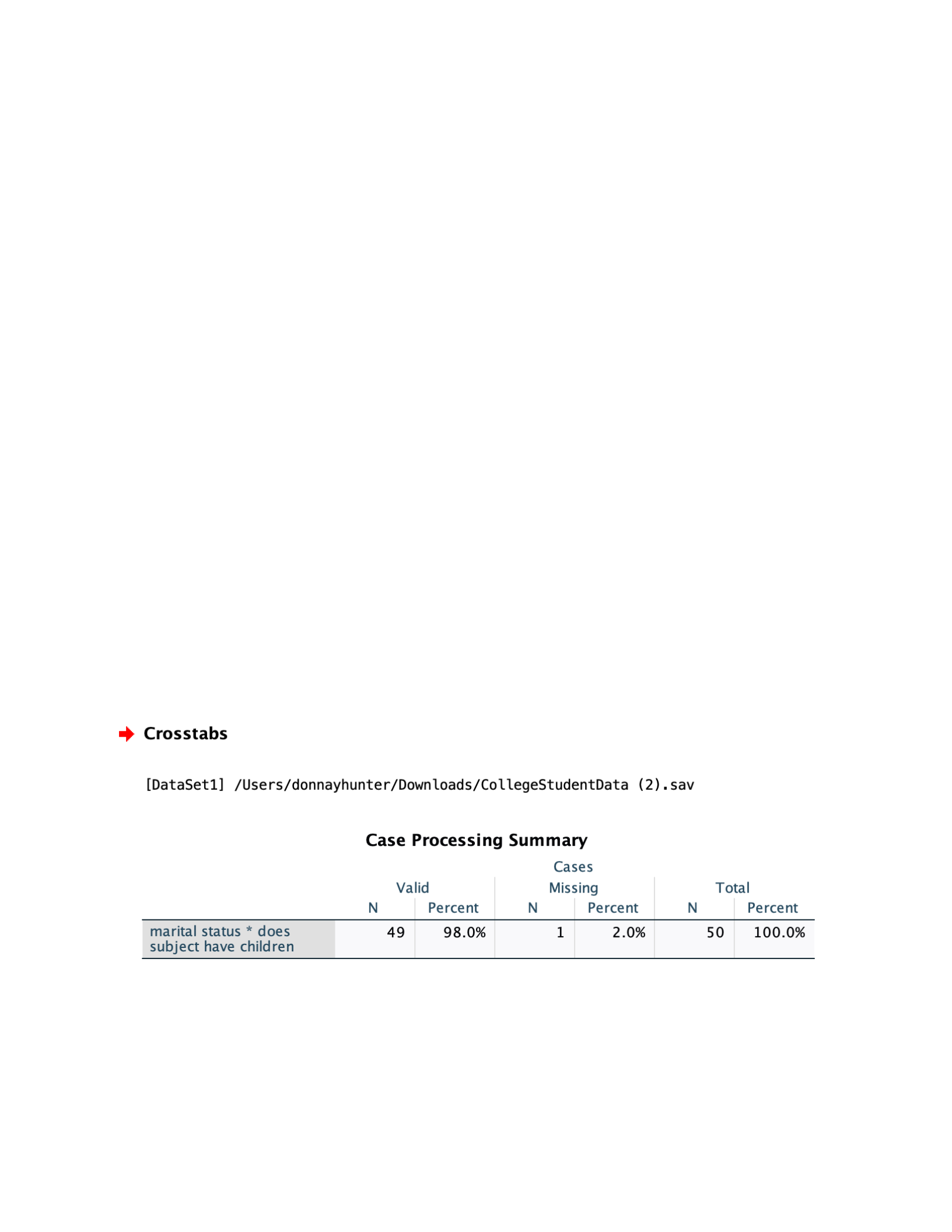
Figure 1.1 shows the Case Processing Summary for having children and marital status
variables. A calculation could not be conducted using the academic track variable as it was not
one of the variables given in the downloaded dataset. The N listed is 49, showing that 49 out of
50 provided data for this question, with 1 missing. Figure 1.2 shows the cross-tabulation for
these variables. It can be determined from this data that out of 23 participants, 87% or 20 of the
23 are single with no children. 4.3% are married with no children, while 8.7% are divorced with
no children. Out of 26 participants, it is shown that none are single with children, 65.4% are
married with children, and 34.6% are divorced with children.
The expected count for each of these in comparison to the actual count shows whether
fewer or more of the participants met the criteria expected by chance. The footnote of the Chi-
square test in Figure 1.3 shows that 0 cells have an expected count of less than 5, with the
minimum expected count being 5.16. Morgan et al. (2020) stated that this indicates that
conditions are valid for performing the Chi-square test. The Chi-square test results of 38.638
show there is a significant difference between the variables. The p-value (0.000), Cramer’s V
(.888), and Phi (.888) indicate that there is strong evidence supporting marital status’ influence
on whether participants have children or not. The Phi value further indicates that there is a strong
association between the variables and a large effect size, meaning that marital status has a
significant impact on having children or not having children.
Figure 1.1
Marital Status/Having Children Case Processing Summary
Figure 1.2
Marital Status/Having Children Crosstabulation
3
6/15/25
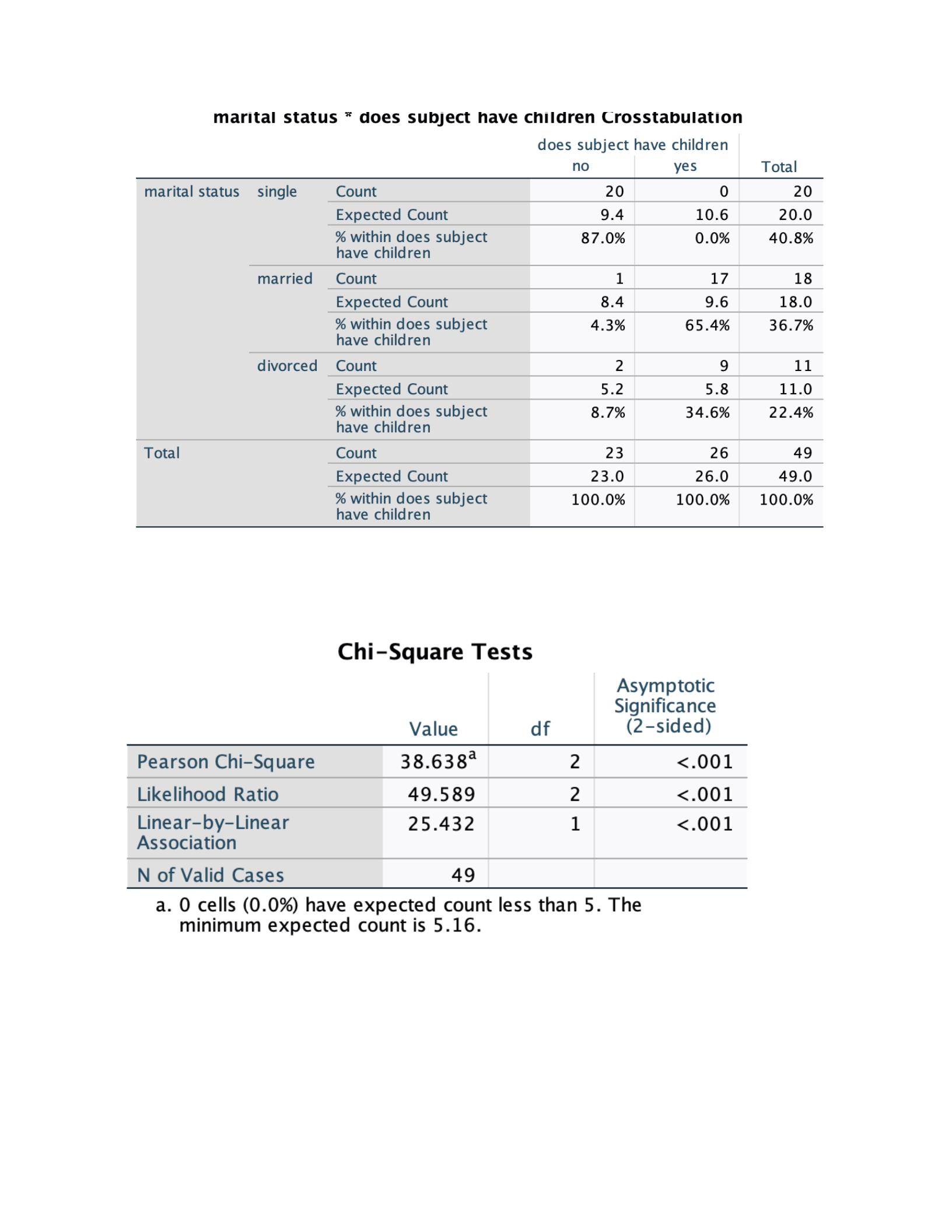
Figure 1.3
Marital Status/Having Children Chi-Square Tests
Figure 1.4
4
6/15/25
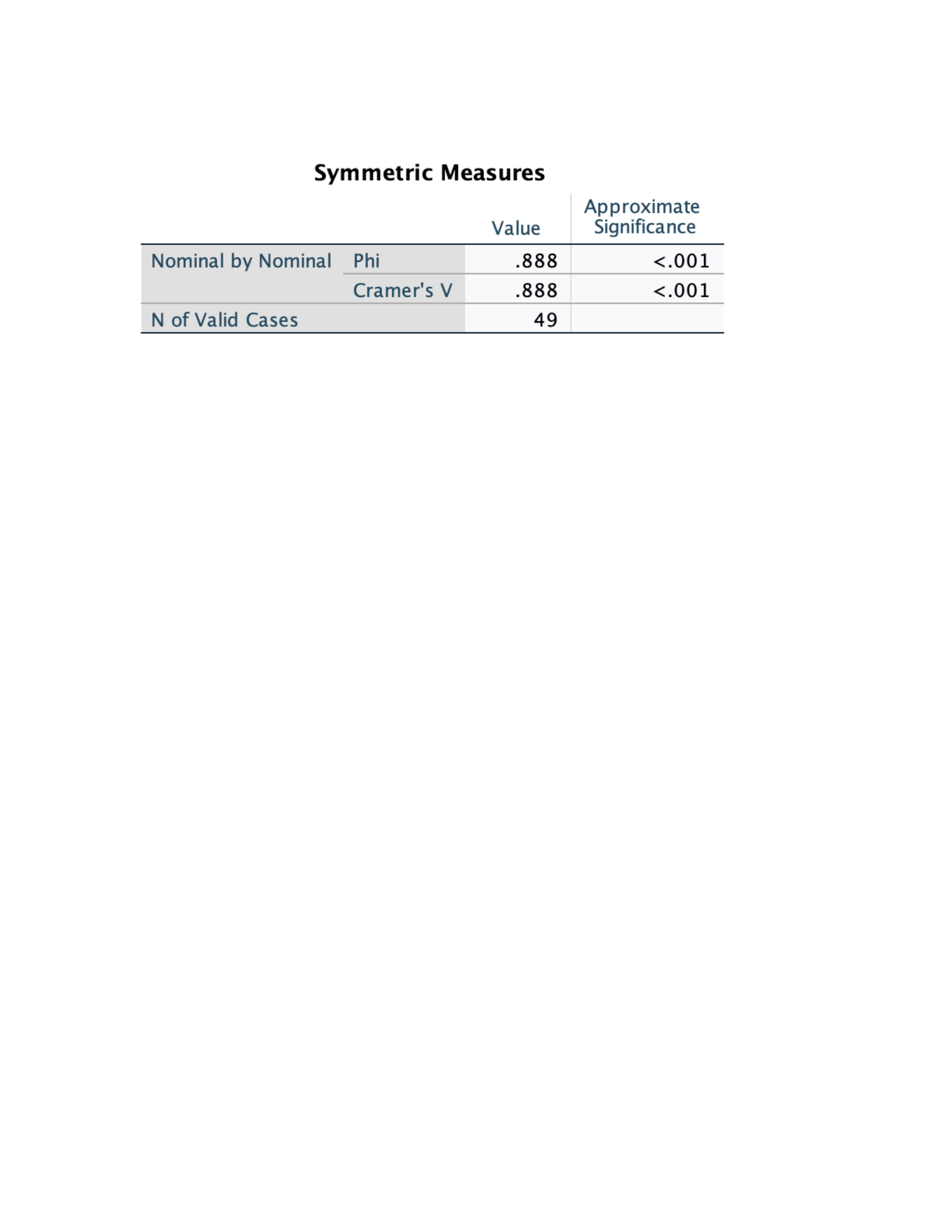
Marital Status/Having Children Symmetric Measures
7.1.b Results for Age Group and Marital Status
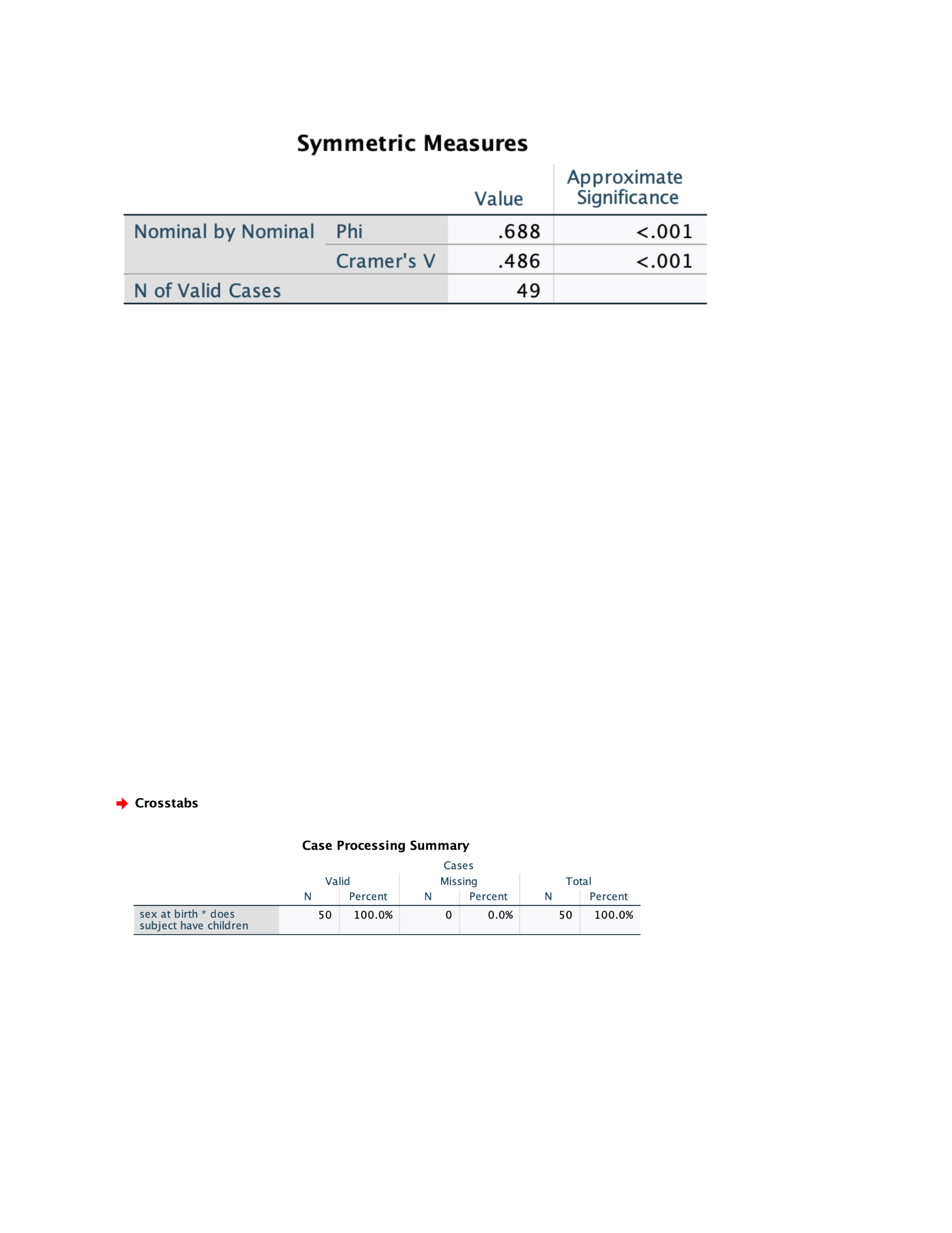
Figure 1.5 show the Case Processing Summary for the variables age group and marital
status, and that there is one case missing, meaning data for one participant is not present. Figure
1.6 shows the Crosstabulation for these variables. Of 16 participants, 13 or 65% are single and
less than 22 years old. Only one is less than 22 years old and married. 2 participants are divorced
and less than 22 years old (18.2%). Out of 18 participants that were between 22-29 years old, one
can see that 7 or 35% of the participants are single, 6 or 33.3% are married, and 5 or 45.4% are
divorced. The crosstabulation also shows that for the participants who are 30 years old or older, 0
are single, 11 or 61.1% are married, and 36.4% or 4 participants are divorced. One could
therefore infer that the older the participant, the more they are married.
The expected counts for these statistics versus the actual count show whether fewer
participants or more participants met the criteria expected by chance (Morgan et al., 2020). The
footnote of the Chi-square test in Figure 1.7 shows that 3 cells or 33.3% have an expected count
of less than 5, and the minimum expected count was 3.37. This means that conditions are invalid
for using the Chi-square test, as 80% of cells need to have an expected count of 5 or higher
(Morgan et al., 2020). The P-value of 0.000 shows strong evidence supporting that agre group
impacts a participant’s likelihood of being married. The chi-square value of 23.173 shows a
significant difference between the two categories. The phi value of .688 also shows a strong
association and large effect size. Therefore, it can strongly be determined that agre group has a
significant impact on participants being married or not.
Figure 1.5
Age Group/Marital Status Case Processing Summary
5
6/15/25
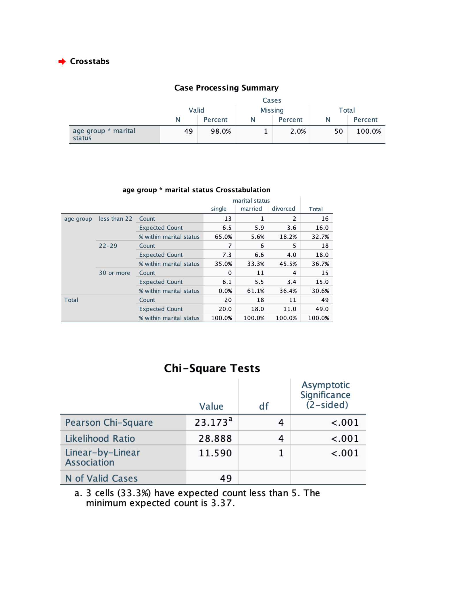
Figure 1.6
Age Group/Marital Status Crosstabulation
Figure 1.7
Age Group/Marital Status Chi-Square Tests
Figure 1.8
Age Group/Marital Status Symmetric Measures
6
6/15/25
7.2 Other Variable Output Interpretations
Two other appropriate variables selected to run and interpret the output as previously
done were sex at birth and does the subject have children. The Case Processing Summary in
Figure 2.1 shows that 50 subjects were involved and no data is missing for these variables.
Figure 2.2 shows that sex at birth males had an actual count of 14 with an expected count of
12.5. When it comes to does subject have children, 58.3% answered no in this category. Figure
2.2 also shows sex at birth males had an actual count of 12 with an expected count of 13.5 for
those who answered yes to having children, 46.2%. Sex at birth females had an actual count of
10 and expected count of 11.5 for those who answered no to having children, which is 41.7%.
Sex at birth females had an actual count of 14 and expected count of 12.5 and answered yes to
having children, which is 53.5%. The chi-square statistic (.742) in Figure 2.3 shows a p value
of .389, which is greater than .05. This means that these variables have no statistical significance
between each other (Morgan et al, 2020). This means there is no true relationship between sex at
birth and subjects having or not having children.
Figure 2.1
Sex at Birth/Does Subject Have Children Case Processing Summary
Figure 2.2
Sex at Birth/Does Subject Have Children Crosstabulation
7
6/15/25
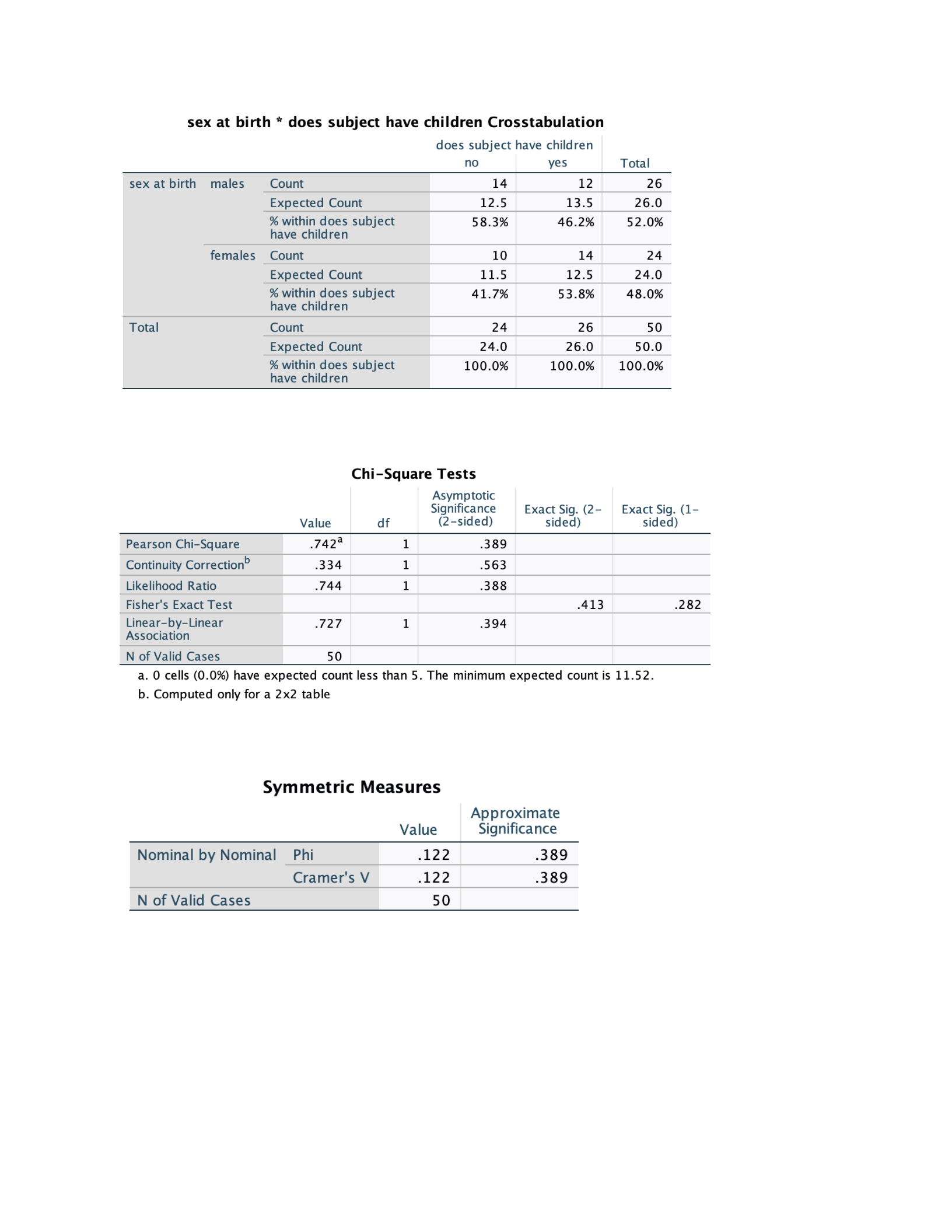
Figure 2.3
Sex at Birth/Does Subject Have Children Chi-Square Tests
Figure 2.4
Sex at Birth/Does Subject Have Children Symmetric Measures
7.3 Association Between Having Children or Not and Watching TV Sitcoms
8
6/15/25
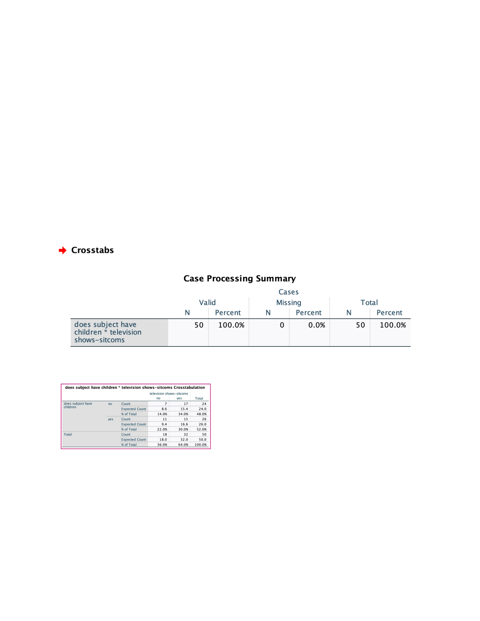
Figure 3.1 shows the Case Processing Summary of subject having children or not and
watching TV sitcoms. This table shows that there is no data missing and 50 participants.
Cramer’s V is one of the correlation statistics that was developed to help in measuring the
strength of association between two nominal variables, and is a nonparametric statistic used in
cross-tabulated table data (Morgan et al., 2020). Because the variables having children or not and
watching sitcoms are nominal variables, Cramer’s V should be the statistic used to explore the
variables’ association. Kendall’s tau-b should not be used as the variables are not ordinal.
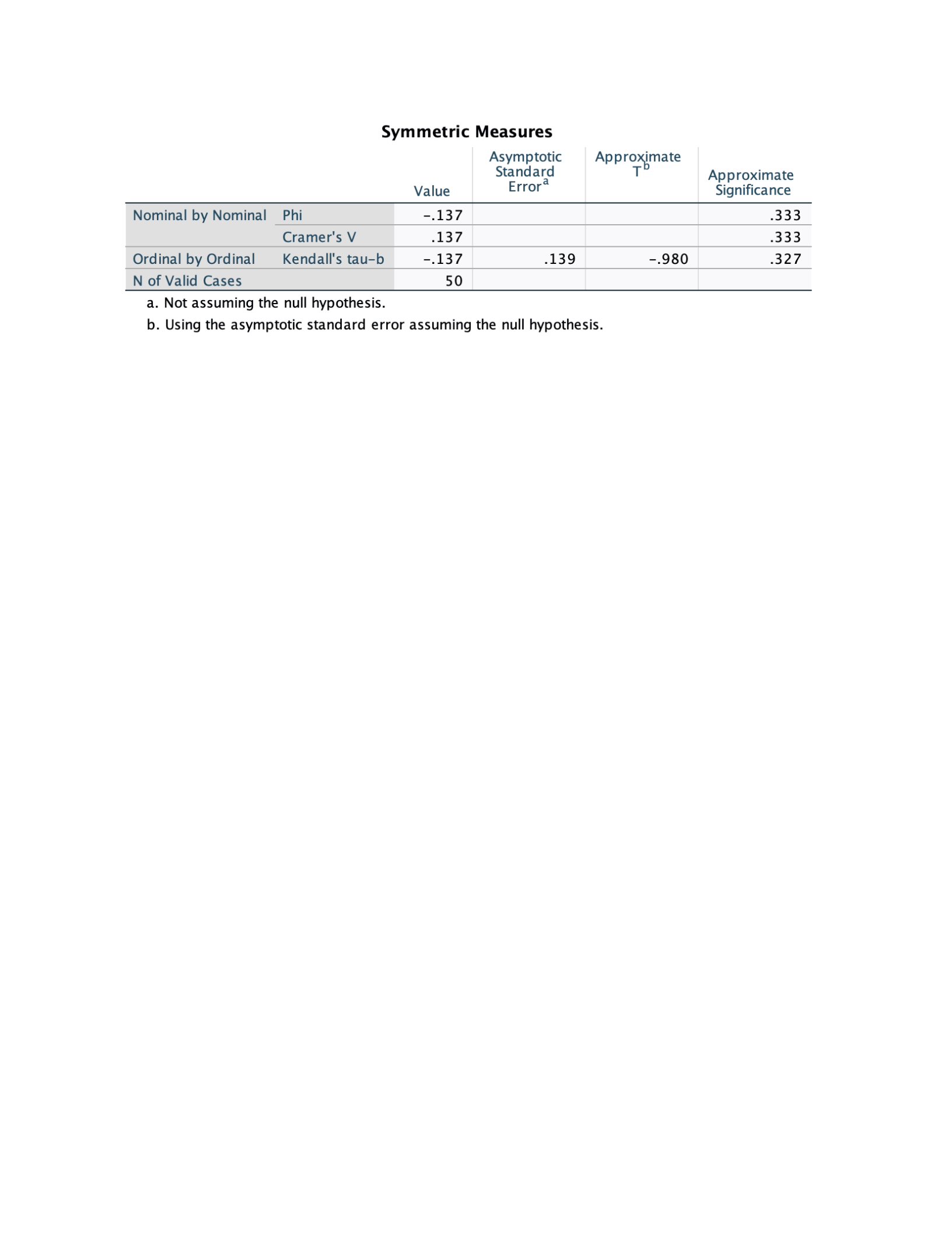
Cramer’s V for this data found in Figure 3.3 is .137, and the approximate significance is .333. A
strong relationship is present if Cramer’s V is greater than +/- 0.25 (Morgan et al., 2020).
Therefore, the variables have a strong relationship. From Figure 3.2, we see that a higher
percentage of subjects without children (70.8%) watch sitcoms, than those who have children
(57.7%).
Figure 3.1
Does Subject Have Children/Watching TV Sitcoms Case Processing Summary
Figure 3.2
Does Subject Have Children/Watching TV Sitcoms Crosstabulation
Figure 3.3
Does Subject Have Children/Watching TV Sitcoms Symmetric Measures
9
6/15/25
7.4 Difference Between Students Who Have Children/Not and Age Group
Figure 4.1 shows the Case Processing Summary for the variables does subject have
children and age group. According to the summary, no data is missing. Figure 4.2 shows the
crosstabulation between the variables along with count and expected count. In looking at this
information, it can be seen that of those younger than 22 years old, 14 do not have children or
82.4%. In those 22-29 years old, 7 do not have children or 38.9%. Of those 30 years old or older,
only 3 do not have children or 20%. This leaves those who are less than 22 years old, 3 of them
have children. 11 students who are in the 22-29 year old age group have children. For those who
are 30 years old or older, 12 of them have children.
The Chi-square test results in Figure 4.3 suggest that there is a strong statistically
significant relationship between having children and age group. The Chi-square value of 13.348
with a p-value of 0.001 shows that the results are statistically significant (since the p value is less
than .05) (Morgan et al., 2020). Cramer’s V in Figure 4.4 further indicates with its .517 value a
moderate to strong association between the variables. Morgan et al. (2020) stated that values near
0 have a week association, while values near 1 have a strong association. Students who have
children are most likely to be in the 30 years old or older age group, while students in the
younger than 22 age group are most likely to not have children.
Figure 4.1
Does Subject Have Children/Age Group Case Processing Summary
10
6/15/25
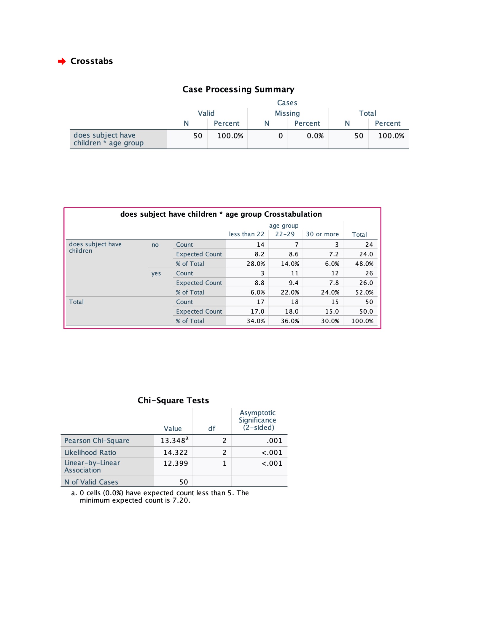
Figure 4.2
Does Subject Have Children/Age Group Crosstabulation
Figure 4.3
Does Subject Have Children/Age Group Chi-Square Tests
Figure 4.4
Does Subject Have Children/Age Group Symmetric Measures
11
6/15/25
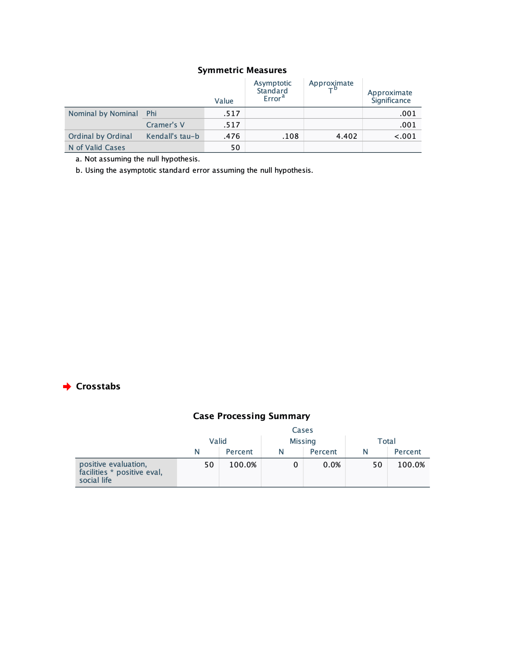
7.5 Appropriate Statistic Computation and Effect Size Measure
Figures 5.2 and 5.3 show the Crosstabulation, Chi-Square test, and Symmetric Measures
for positive evaluation of social life and positive evaluation of facilities, as academic track was
not given in the dataset. Both of these variables are ordinal data, making Kendall’s tau-b the
most appropriate form of measure. The p-value is greater than .001 (0.257) and Kendall’s tau-b
is –0.134, indicating that it is not statistically significant. The negative value of Kendall’s tau-b
suggests that there is a week negative relationship. Since it is not significant, no meaningful
association can be recognized (Morgan et al., 2020). The effect size could then be determined
weak, as these results do not support a strong/reliable correlation between the variables.
Figure 5.1
Positive Eval of Social Life and Positive Eval of Facilities Case Processing Summary
Figure 5.2
Positive Eval of Social Life and Positive Eval of Facilities Crosstabulation
12
6/15/25
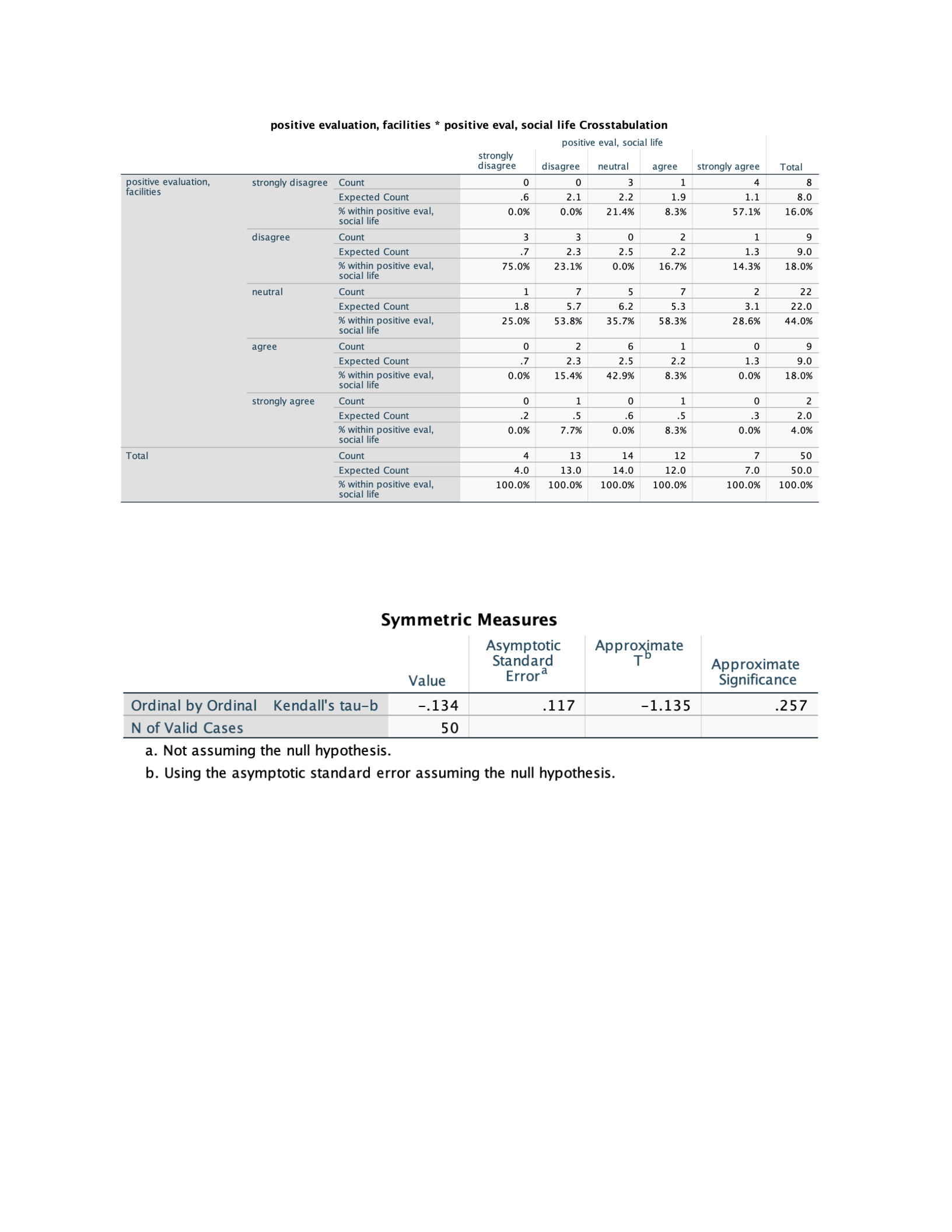
Figure 5.3
Positive Eval of Social Life and Positive Eval of Facilities Symmetric Measures
References
13
6/15/25

Morgan, G., Leech, N., Gloeckner, G., Barrett, K. (2020). IBM SPSS for Introductory Statistics
(5th Ed.). New York, NY
14
6/15/25

