


Fuel Consumption
Analysis
F Consumption
A
TEAM 6
TEAM 6
Introduction to Fuel Consumption
Introduction to Fuel Consumption
●The data set included information gathered from one vehicle and driver
over the course of a few months
●Data includes gas consumed, distance driven, average speed, weather
(sun and rain), air conditioning (on or off), temperature outside vehicle,
temperature inside vehicle, and the gas type used (E10 or SP98)
●Goal of analysis was to find correlations, if any, between gas consumed
and the other variables recorded
●The data set was chosen by our group because we wanted to explore
opportunity to reduce fuel consumption as it pertains to our lives
O D
Variables:
●Gas consumed: litre/100km (consume)
●Distance: km (distance)
●Average Speed: km/hr (speed)
●Inside Temperature: Celcius (temp_inside)
●Outside Temperature: Celcius (temp_outside)
●Sun and Rain: present or absent
●Gas Type: E10 or SP98
●Air Conditioning: present or absent
●Our goal was to find possible correlations between the
independent variables and the dependent variable of
gas consumed
V :
●G con : litr /100km (con )
●D : km (distanc )
●A S : km/h (speed)
●I T : C (te _inside)
●O T : C (temp_ )
●S an Rain: p or a
●G T : E10 SP98
●A Co : or
●O goa was to find pos cor the
va a the depen va
cons

A C
Our first step was performing data cleaning. We sorted our data into three spreadsheets,
one for each model. We performed a multivariate analysis and ran an outlier analysis to
visually identify outliers above the threshold. We excluded those data points and added
imputed data for our empty data fields.
O first step wa performing data cleani . W sorted our into spreadsheets,
for ea model. W perfo a multi an a ran an outli anal to
identify outli above the threshold. W ex those da points and
dat for our empty da fields.
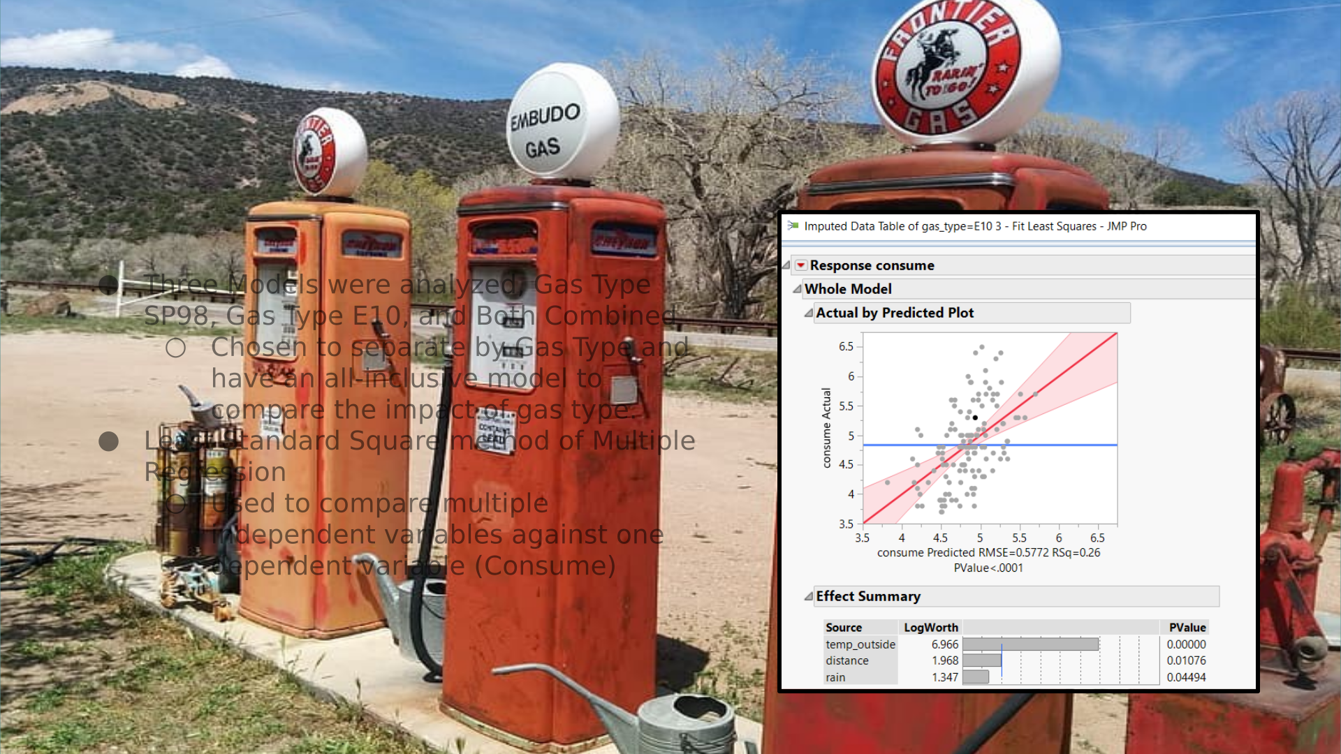
●Three Models were analyzed, Gas Type
SP98, Gas Type E10, and Both Combined
○Chosen to separate by Gas Type and
have an all-inclusive model to
compare the impact of gas type.
●Least Standard Square method of Multiple
Regression
○Used to compare multiple
independent variables against one
dependent variable (Consume)
●T Models were analyzed, Gas T
SP98, G T E10, and Bo Combined
○C to by G T
an al -inclusi model to
the impact of ga type.
●L Standard Squar met of Multip
R
○U to multiple
va ag one
vari (Con )
A C E10 M
E
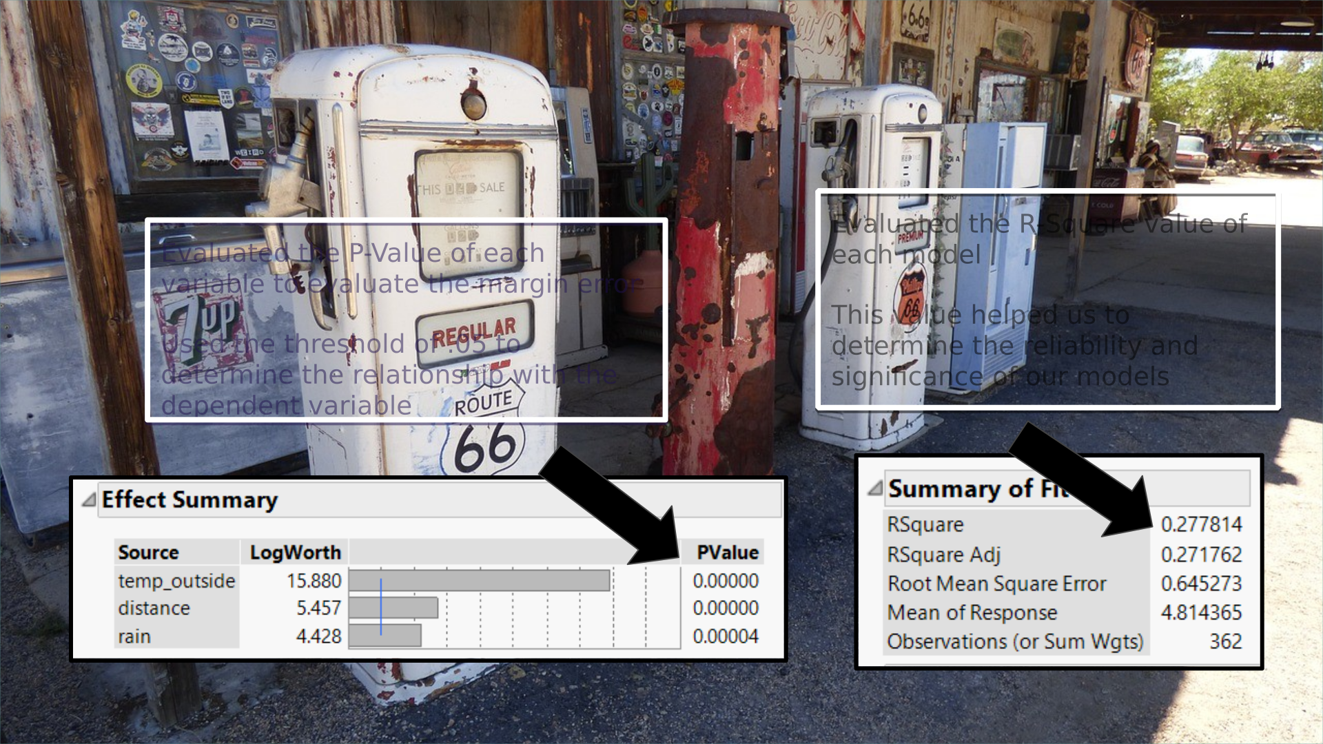
Evaluated the R-Square value of
each model
This value helped us to
determine the reliability and
significance of our models
E the R-S value of
model
T value hel us to
the reliabi and
o our models
A C
Evaluated the P-Value of each
variable to evaluate the margin error
Used the threshold of .05 to
determine the relationship with the
dependent variable
E the P-V of ea
to eval the margin err
U the threshold of .05 to
the relationship w the
vari
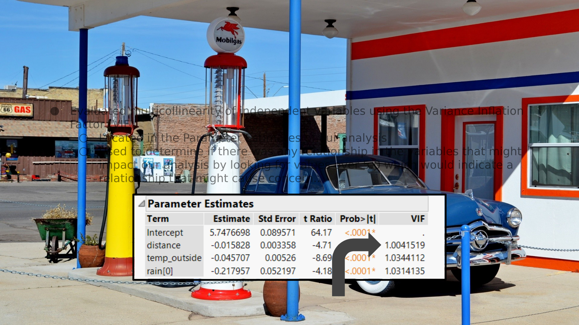
●Evaluated multicollinearity of independent variables using the Variance Inflation
Factor (VIF)
○Located in the Parameter Estimates of our analysis
○Used to determine if there was any relationship in the variables that might
impact our analysis by looking for values over 5.0 which would indicate a
relationship that might cause concern..
●E multicol of independen variabl using the V Infla
F (VIF)
○L in the P Estimat of our anal
○U to determine if there was any relatio in the va might
our anal by l for ove 5.0 which woul indicate a
that m cause concern..
A C
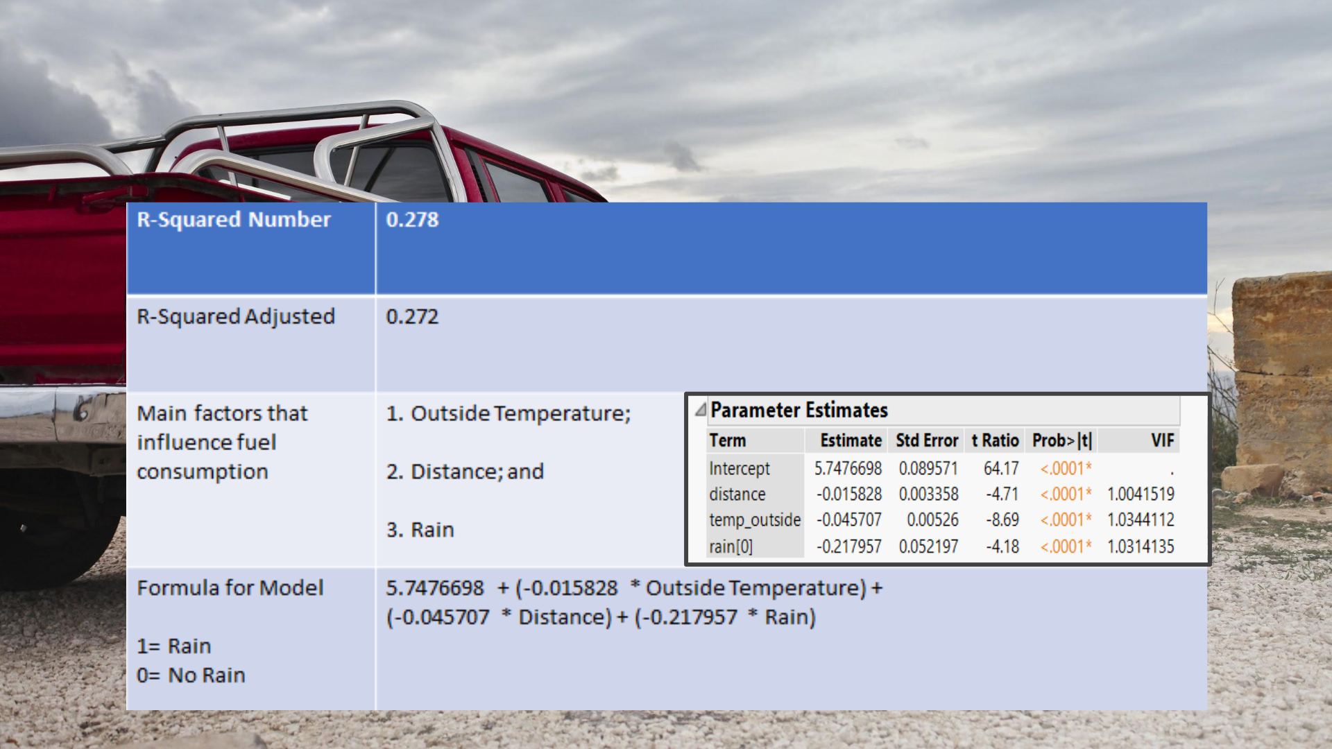
R f SP98 and E10 Mo
R f Combined Model
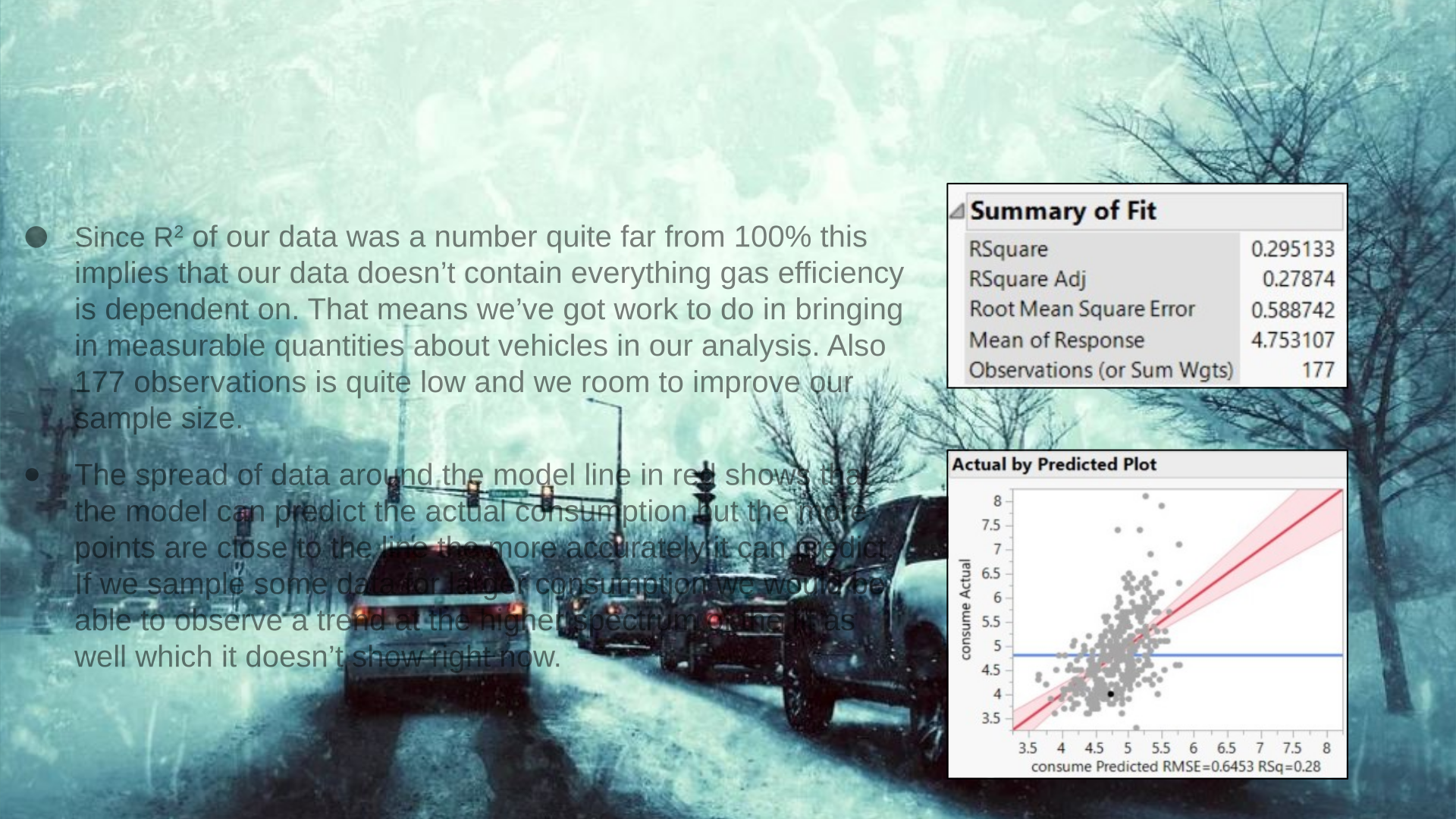
●Since R2 of our data was a number quite far from 100% this
implies that our data doesn’t contain everything gas efficiency
is dependent on. That means we’ve got work to do in bringing
in measurable quantities about vehicles in our analysis. Also
177 observations is quite low and we room to improve our
sample size.
●The spread of data around the model line in red shows that
the model can predict the actual consumption but the more
points are close to the line the more accurately it can predict.
If we sample some data for larger consumption we would be
able to observe a trend at the higher spectrum of the fit as
well which it doesn’t show right now.
●S R2 our dat was a q far 100%
th our d doe ’t c gas
depe o . T means ’ve go work to in
measu q vehicl in o an . A
177 is lo and we roo to impro ou
si .
●T spre of d arou the lin in red t
model p th actu cons the
clo to th line t more a it pr .
I we sampl some da for l we be
to o a tren at the spectr of t fit as
which i doesn’ sho right n .
I and
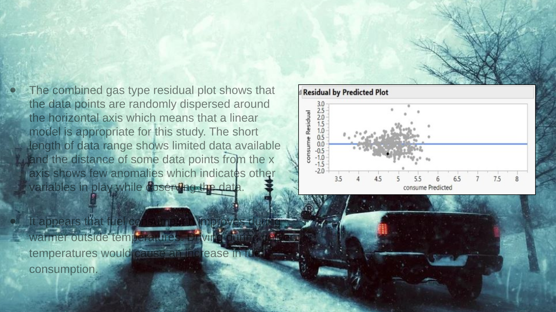
●The combined gas type residual plot shows that
the data points are randomly dispersed around
the horizontal axis which means that a linear
model is appropriate for this study. The short
length of data range shows limited data available
and the distance of some data points from the x
axis shows few anomalies which indicates other
variables in play while observing the data.
●T comb gas r plot s that
data points are randoml dispersed around
hori axis whi means a
is fo this . T sh
data s limit data
the of data the
sh few an indi o
in while the .
I and
●It appears that fuel consumption improves during
warmer outside temperatures. Driving during colder
temperatures would cause an increase in fuel
consumption.
●I appe tha fuel c improve duri
outs tempe . Drivin durin colde
would an inc fuel
.

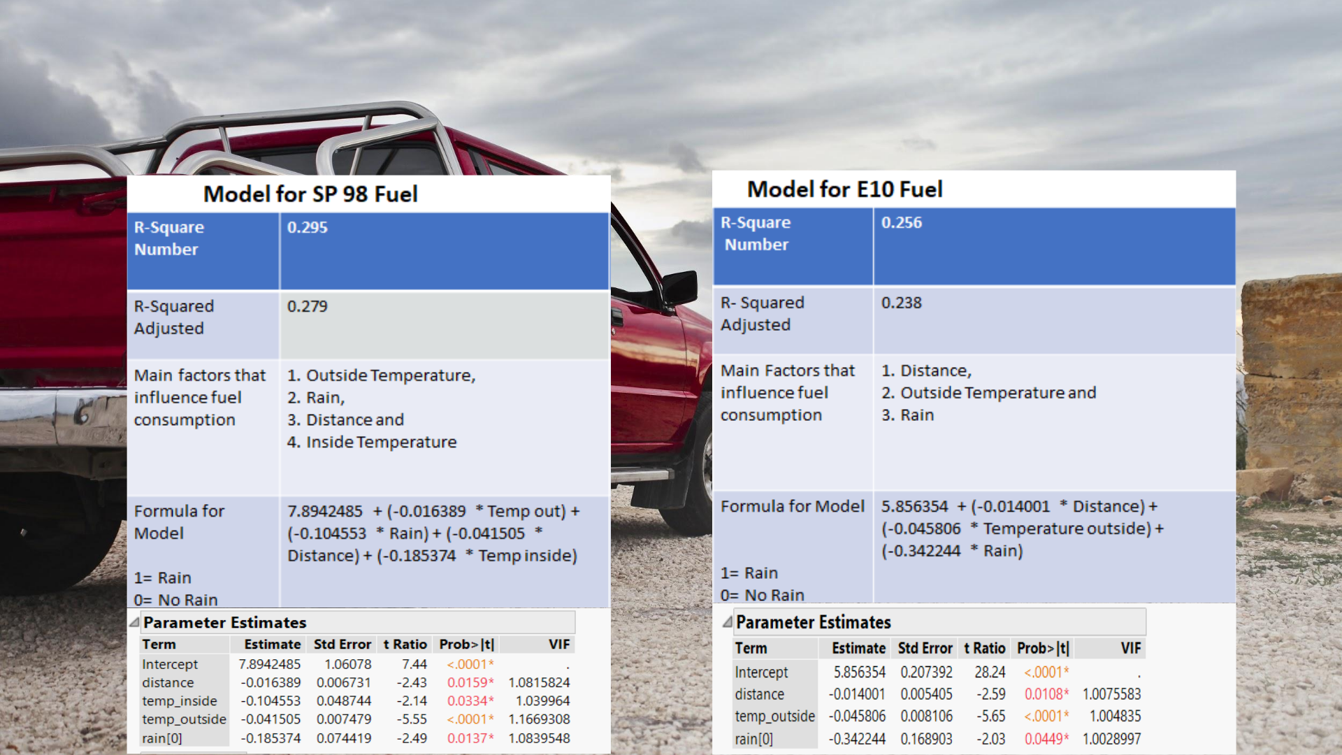
○The temperature outside seemed to have a higher negative correlation with consumption for
Gas Type E10, but E10 Gas was tested during warmer weather and SP98 in the winter.1
Running the analysis again but switching the Gas Types might give additional clarity on
whether the Gas Type used changes the impact of our variables.
○Rain also had a higher impact on consumption for our E10 gas model. Rain might occur
more often during the time of year that E10 gas was tested.
○T temperature see to have higher negat corr with f
G T E10, but E10 G t during warm weather and SP98 t winter.1
R the analy again switc the G T giv additional c
the G T ch the impact variables.
○R also had higher impact cons for E10 gas . Rain might
often d the t of y that E10 tes .
D ’t Speed just yet...
●Interesting findings
○We expected to see much higher r-square values,
particularly from including speed. However, speed did not
end up even being a variable with a low enough P-Value
in any of our models.
●I findings
○W s much higher r- va ,
inclu speed. H , did not
up even be a var with a low P-V
any of models.
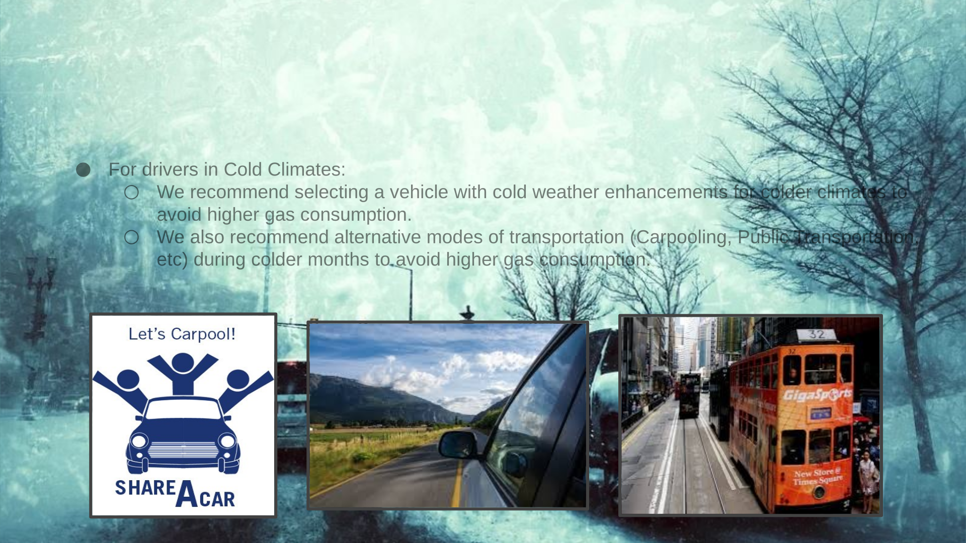
●For drivers in Cold Climates:
○We recommend selecting a vehicle with cold weather enhancements for colder climates to
avoid higher gas consumption.
○We also recommend alternative modes of transportation (Carpooling, Public Transportation,
etc) during colder months to avoid higher gas consumption.
●F drivers Cold Climates:
○W recommend selecting vehicle cold enhancement for cli t
higher cons .
○W also recommend alternati modes t (Carpooling, Public T ,
) dur colder months higher gas .
R
●Additional Testing Recommended
○Bring in additional variables that contribute to
gas consumption would provide improved data
results. These additional variables include:
○Increase sample size of the data from more
than one vehicle.
○These changes would all have an effect on our
R-squared value and further show that our
model can predict fuel consumption in vehicles
based on the correct attributes.
●A T Recommended
○B in addit variables t
cons would prov improved data
. T additional v inc :
○I size t data more
one .
○T changes all have effect on our
R- value and that
can predic fuel in vehicles
on t correct .
R


