


Practical Exam Review
WPC 300
Dr. Asish Satpathy
3/7/21 1Dr. Asish Satpathy

Excel (Descriptive data analysis)
•Excel functions (including math functions)
•Vlookup function
•Pivot table operations
•Data visualization
•Example:
•StudentGrade.xlsx
•Room Rate.xlsx
3/7/21 2Dr. Asish Satpathy
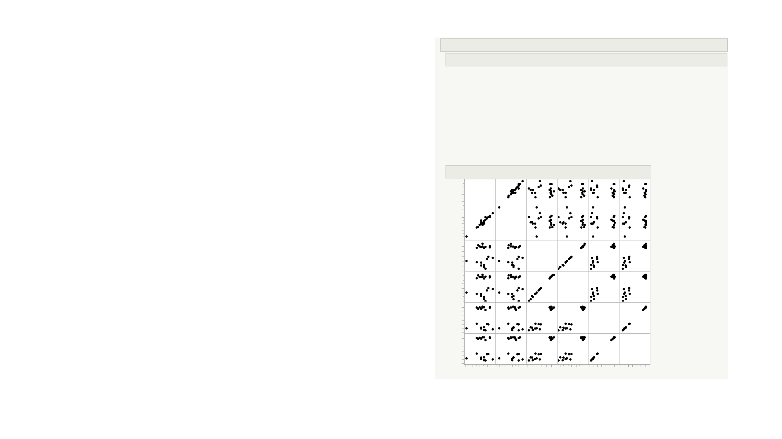
JMP (data correlations):
•Analyze -> Multivariate ->
Multivariate Methods
•Correlation between
continuous data variables:
•Value: -1<r<1
•No correlation when r=0
•Data: Colestrol.jmp
Multivariate
Correlations
April AM
April PM
May AM
May PM
June AM
June PM
1.0000
0.9657
0.0681
0.0695
0.0232
0.0251
0.9657
1.0000
0.0268
0.0331
-0.0028
-0.0003
0.0681
0.0268
1.0000
0.9989
0.9545
0.9555
0.0695
0.0331
0.9989
1.0000
0.9559
0.9570
0.0232
-0.0028
0.9545
0.9559
1.0000
0.9997
0.0251
-0.0003
0.9555
0.9570
0.9997
1.0000
April AM April PM May AM May PM June AM June PM
The correlations are estimated by Row-wise
method.
Scatterplot Matrix
265
270
275
280
270
275
280
285
180
220
260
200
220
240
260
280
160
200
240
280
160
200
240
280
April AM
270 285
April PM
270 290
May AM
200 260
May PM
200 260
June AM
180 260
June PM
180 260
3/7/21 3Dr. Asish Satpathy
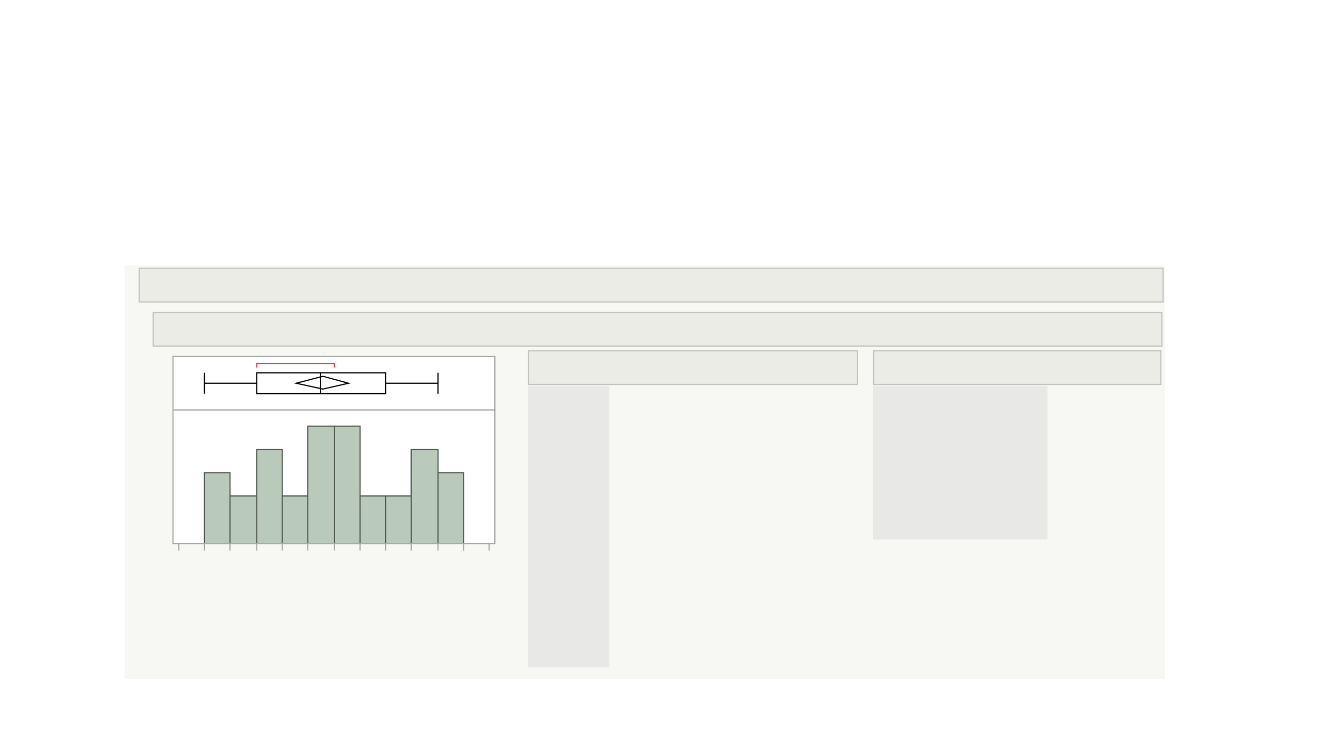
JMP (Data visualization –summary statistics)
•Analyze -> Distribution Data: Drug Measurement.jmp
Distributions
Measurement
90 92 94 96 98 100 102
Quantiles
100.0%
99.5%
97.5%
90.0%
75.0%
50.0%
25.0%
10.0%
2.5%
0.5%
0.0%
maximum
quartile
median
quartile
minimum
100
100
100
99.7
98
95.5
93
91.3
91
91
91
Summary Statistics
Mean
Std Dev
Std Err Mean
Upper 95% Mean
Lower 95% Mean
N
95.5625
2.8048058
0.4958243
96.57374
94.55126
32
3/7/21 4Dr. Asish Satpathy
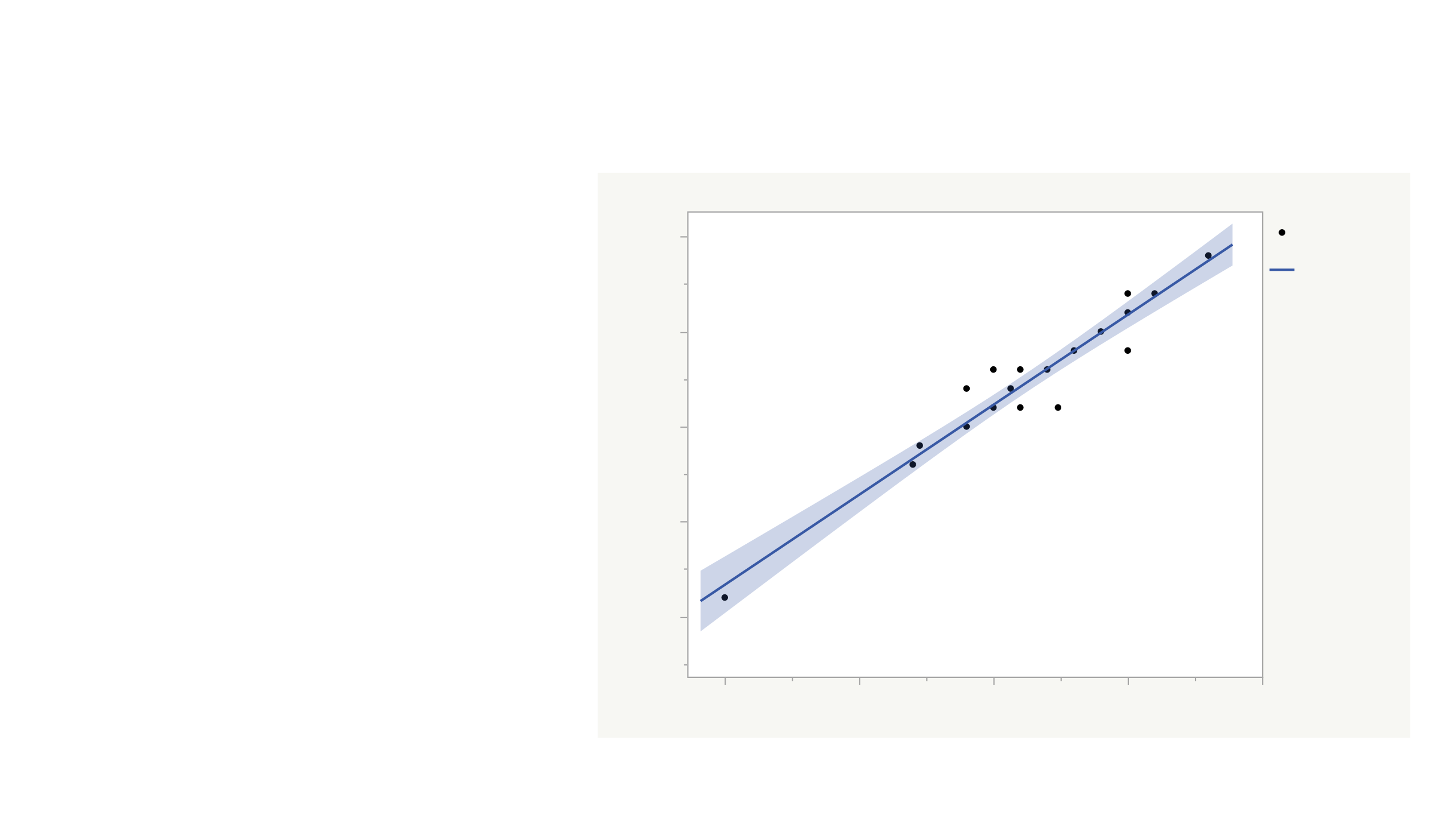
JMP (Data visualization: Graph builder)
•Graph -> Graph builder
•Data: Colestrol.jmp
April AM vs. April PM
April PM
270 275 280 285 290
April AM
265
270
275
280
285
Y = 10.8 + 0.9477*X
R²: 0.933
April AM
April AM
3/7/21 5Dr. Asish Satpathy
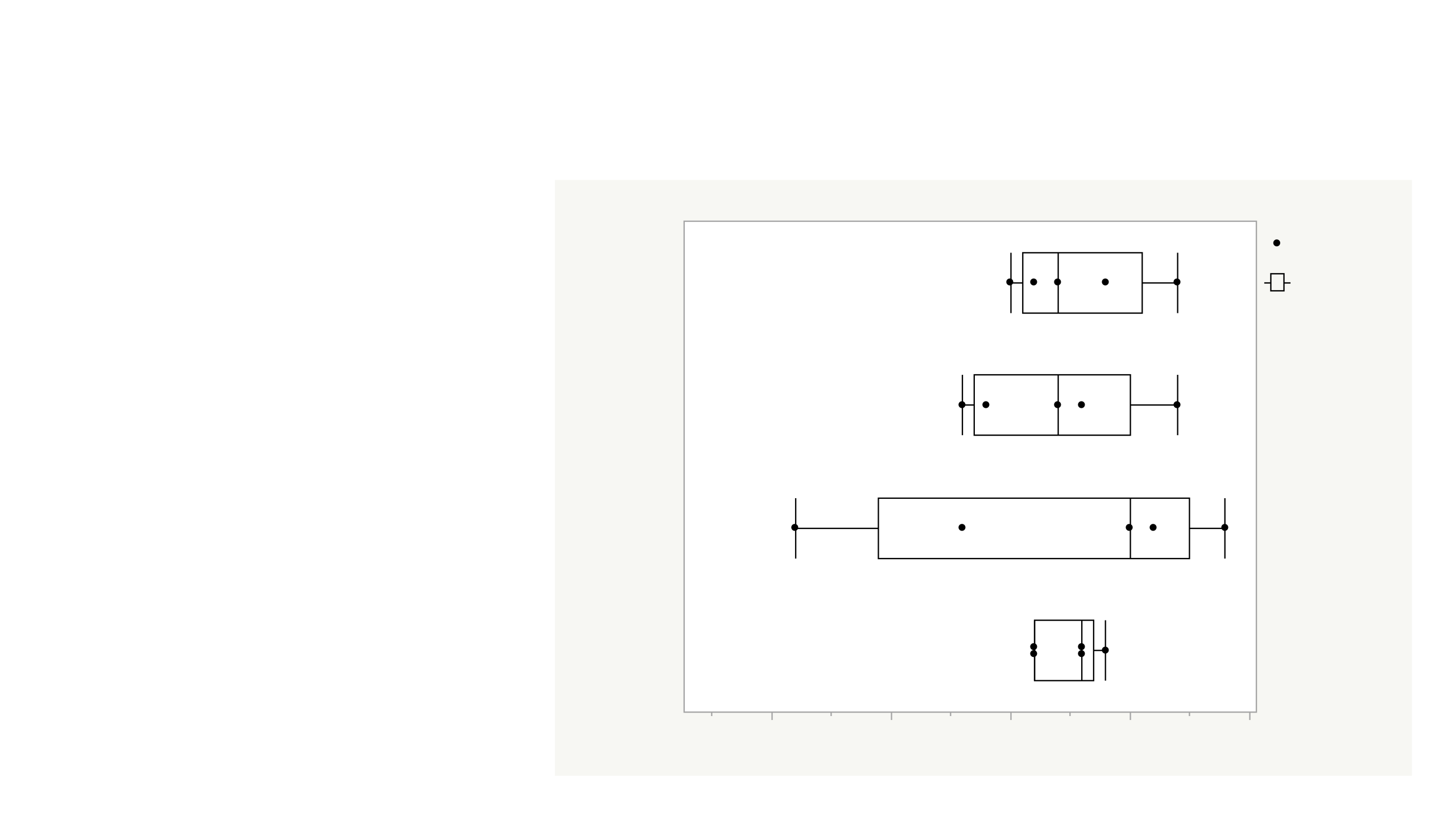
JMP (Data visualization: Graph builder)
•Graph -> Graph builder
•Data: Colestrol.jmp
April AM vs. treatment
April AM
265 270 275 280 285
treatment
A
B
Control
Placebo
April AM
April AM
3/7/21 6Dr. Asish Satpathy
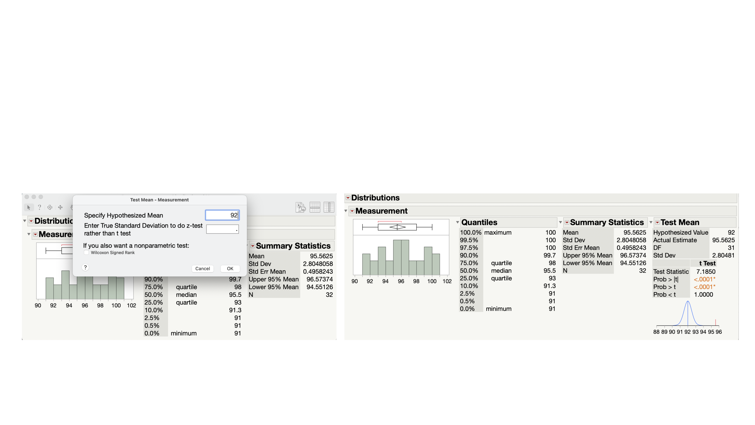
JMP (Inferential analysis): t-test
•Comparing a mean with another mean or number
•Analyze -> Distribution -> Test mean | Data: Drug Measurement.jmp
3/7/21 7Dr. Asish Satpathy
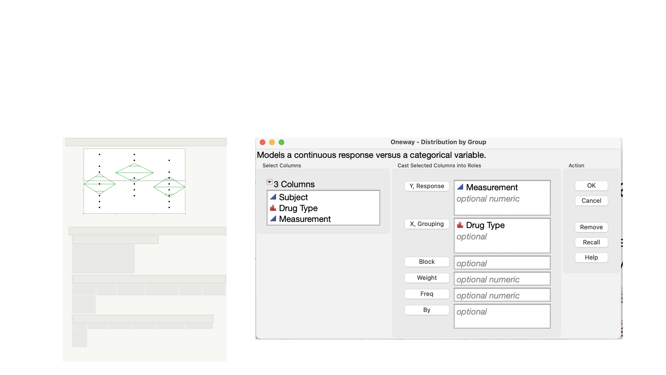
JMP (Inferential analysis): ANOVA
•Comparing multiple means with one another
•Analyze -> Fit y by x -> Means/ANOVA (perform Tukey if you reject null)
Oneway Analysis of Measurement By Drug Type
90
92
94
96
98
100
Measurement
abc
Drug Type
Oneway Anova
Summary of Fit
Rsquare
Adj Rsquare
Root Mean Square Error
Mean of Response
Observations (or Sum Wgts)
0.149496
0.090841
2.674378
95.5625
32
Analysis of Variance
Source
Drug Type
Error
C. Total
DF
2
29
31
Sum of
Squares
36.45833
207.41667
243.87500
Mean Square
18.2292
7.1523
F Ratio
2.5487
Prob > F
0.0956
Means for Oneway Anova
Level
a
b
c
Number
10
12
10
Mean
95.0000
96.9167
94.5000
Std Error
0.84571
0.77203
0.84571
Lower 95%
93.270
95.338
92.770
Upper 95%
96.730
98.496
96.230
Std Error uses a pooled estimate of error
variance
3/7/21 8Dr. Asish Satpathy
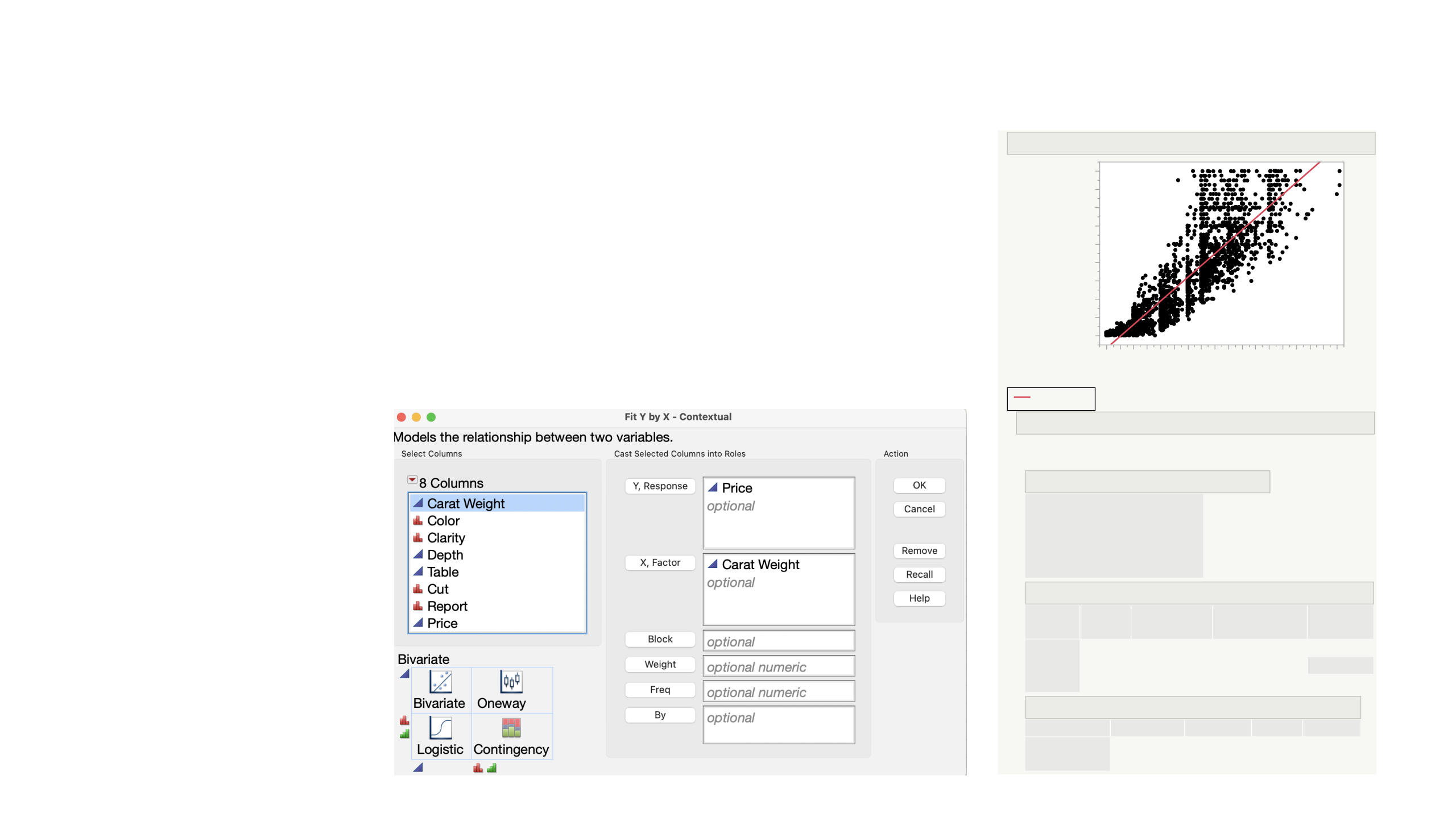
JMP (Inferential analysis): Simple Linear
Regression
•Simple Linear Regression:
•Analyze -> Fit Y by X (both x & y continuous) -> Fit line
•Y (depended variable or response variable), X
(independent variable)
•Data:
•Diamonds Data.jmp
Bivariate Fit of Price By Carat Weight
$1,000.00
$2,000.00
$3,000.00
$4,000.00
$5,000.00
$6,000.00
$7,000.00
$8,000.00
$9,000.00
$10,000.00
Price
0.3 0.5 0.7 0.9 1.1 1.3 1.5 1.7 1.9
Carat Weight
Linear Fit
Linear Fit
Price = -1660.618 + 6472.8914*Carat
Weight
Summary of Fit
RSquare
RSquare Adj
Root Mean Square Error
Mean of Response
Observations (or Sum Wgts)
0.742595
0.742499
1228.137
3971.471
2690
Analysis of Variance
Source
Model
Error
C. Total
DF
1
2688
2689
Sum of
Squares
1.1697e+10
4054363555
1.5751e+10
Mean Square
1.17e+10
1508319.8
F Ratio
7754.685
Prob > F
<.0001*
Parameter Estimates
Term
Intercept
Carat Weight
Estimate
-1660.618
6472.8914
Std Error
68.19971
73.50489
t Ratio
-24.35
88.06
Prob>|t|
<.0001*
<.0001*
3/7/21 9Dr. Asish Satpathy
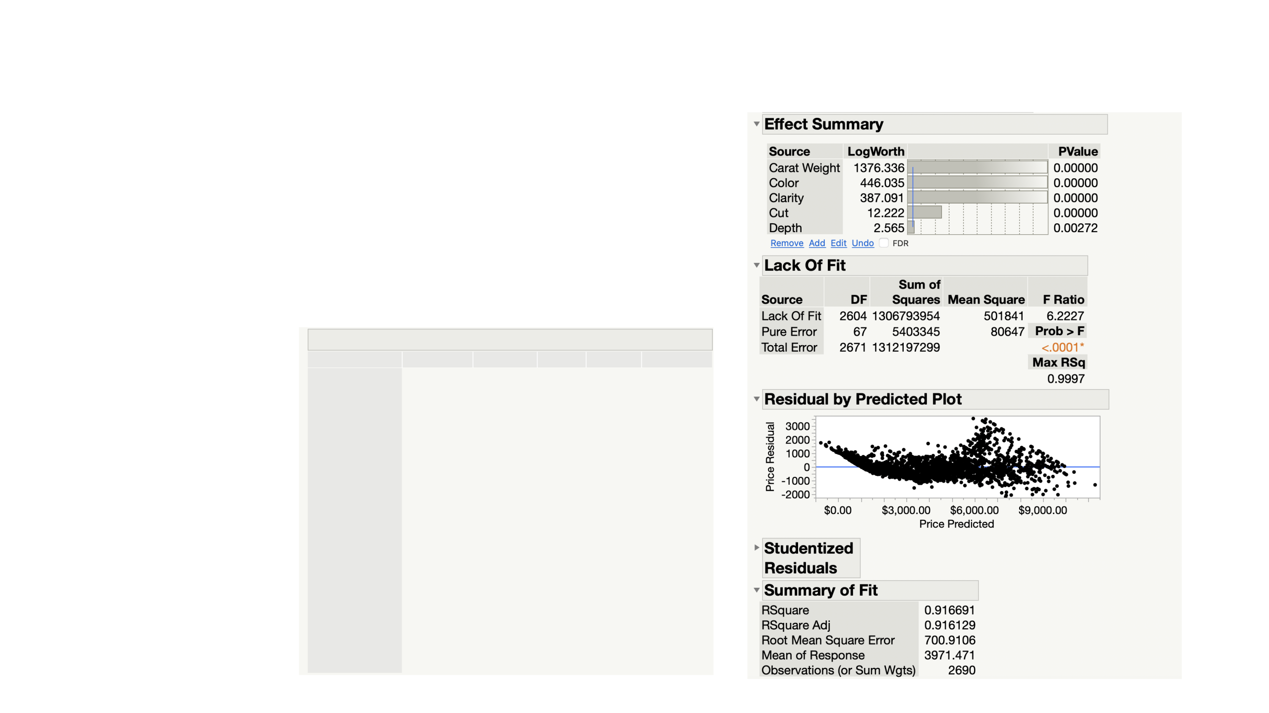
JMP (Inferential analysis): Multiple Linear
Regression
•Analyze -> Fit Model
•Y (depended variable or response variable)
•Model effects (multiple independent
variables)
•Use
Diamonds Data.jmp
Parameter Estimates
Term
Intercept
Carat Weight
Color[K]
Color[J]
Color[I]
Color[H]
Color[G]
Color[F]
Color[E]
Clarity[SI2]
Clarity[SI1]
Clarity[VS2]
Clarity[VS1]
Clarity[VVS2]
Clarity[VVS1]
Depth
Cut[Good]
Cut[Very Good]
Cut[Excellent]
Estimate
-1620.112
8824.0147
-2106.078
-1199.446
-448.1703
153.57419
676.65615
830.44771
933.57226
-1486.161
-786.9519
-116.9292
332.01148
497.30893
627.3794
-34.1315
-272.3182
-49.04955
67.584276
Std Error
703.0726
54.83078
59.38346
42.18251
38.02895
34.2892
34.05869
33.71472
32.9606
32.83164
29.5642
31.93696
33.69835
39.47525
41.03295
11.37537
43.92181
25.92011
24.55859
t Ratio
-2.30
160.93
-35.47
-28.43
-11.78
4.48
19.87
24.63
28.32
-45.27
-26.62
-3.66
9.85
12.60
15.29
-3.00
-6.20
-1.89
2.75
Prob>|t|
0.0213*
<.0001*
<.0001*
<.0001*
<.0001*
<.0001*
<.0001*
<.0001*
<.0001*
<.0001*
<.0001*
0.0003*
<.0001*
<.0001*
<.0001*
0.0027*
<.0001*
0.0586
0.0060*
VIF
.
1.7083805
2.7758886
1.9188448
1.7439891
1.5936965
1.5766499
1.6177269
1.6847332
1.3573055
1.2139867
1.1769338
1.1861087
1.2973351
1.3955289
1.0371184
1.3737851
1.3152882
1.2504023
3/7/21 10Dr. Asish Satpathy
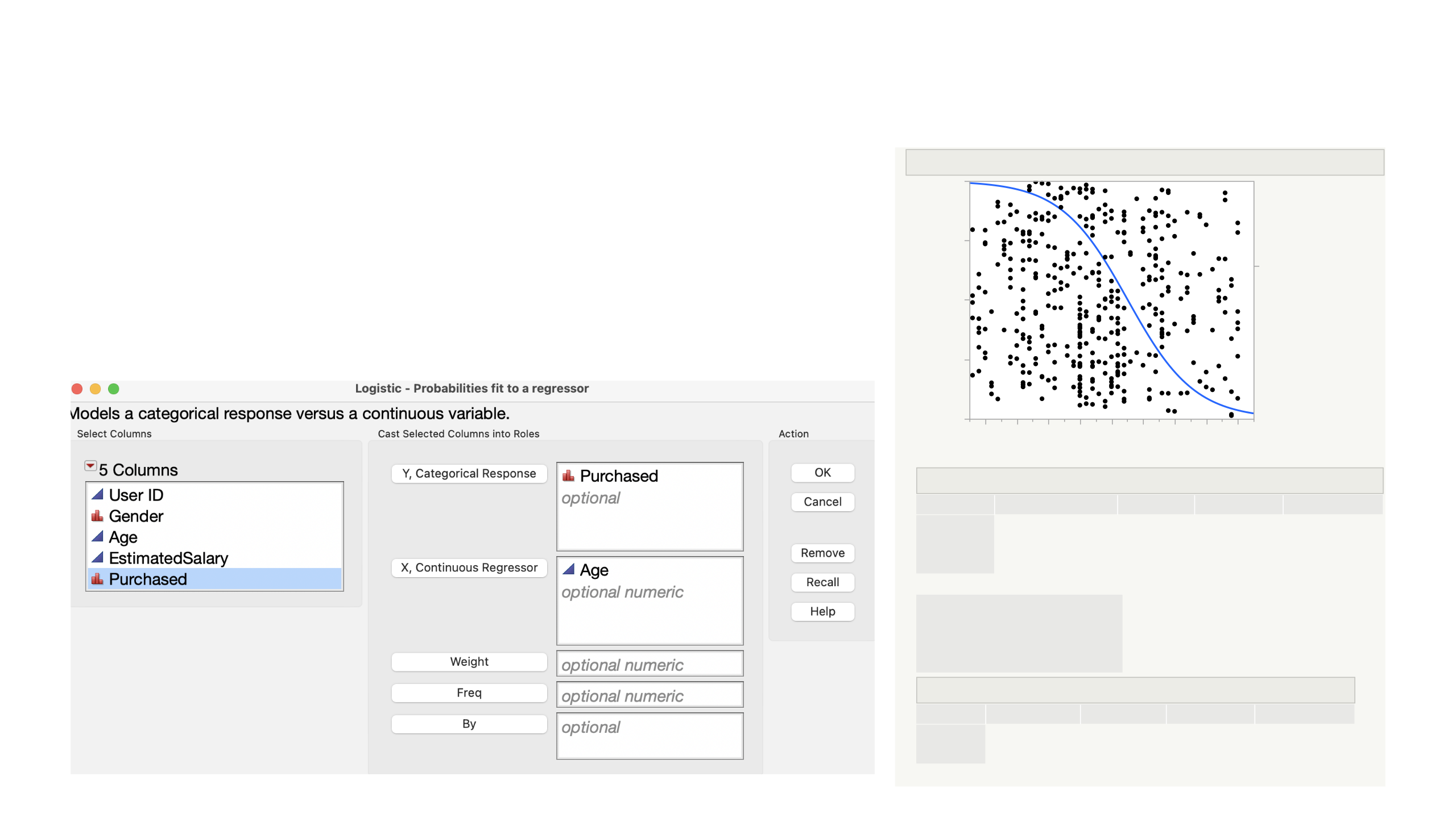
JMP (Inferential analysis): Simple Logistic
Regression
•Analyze -> Fit Y by X (y variable is binary)
•Data: Social_Network_Ads.jmp
Logistic Fit of Purchased By Age
0.00
0.25
0.50
0.75
1.00
Purchased
20 25 30 35 40 45 50 55 60
Age
0
1
Whole Model Test
Model
Difference
Full
Reduced
-LogLikelihood
92.65584
168.13065
260.78648
DF
1
ChiSquare
185.3117
Prob>ChiSq
<.0001*
RSquare (U)
AICc
BIC
Observations (or Sum Wgts)
0.3553
340.292
348.244
400
Parameter Estimates
Term
Intercept
Age
Estimate
8.04414238
-0.1889496
Std Error
0.7841778
0.019152
ChiSquare
105.23
97.33
Prob>ChiSq
<.0001*
<.0001*
For log odds of 0/1
3/7/21 11Dr. Asish Satpathy
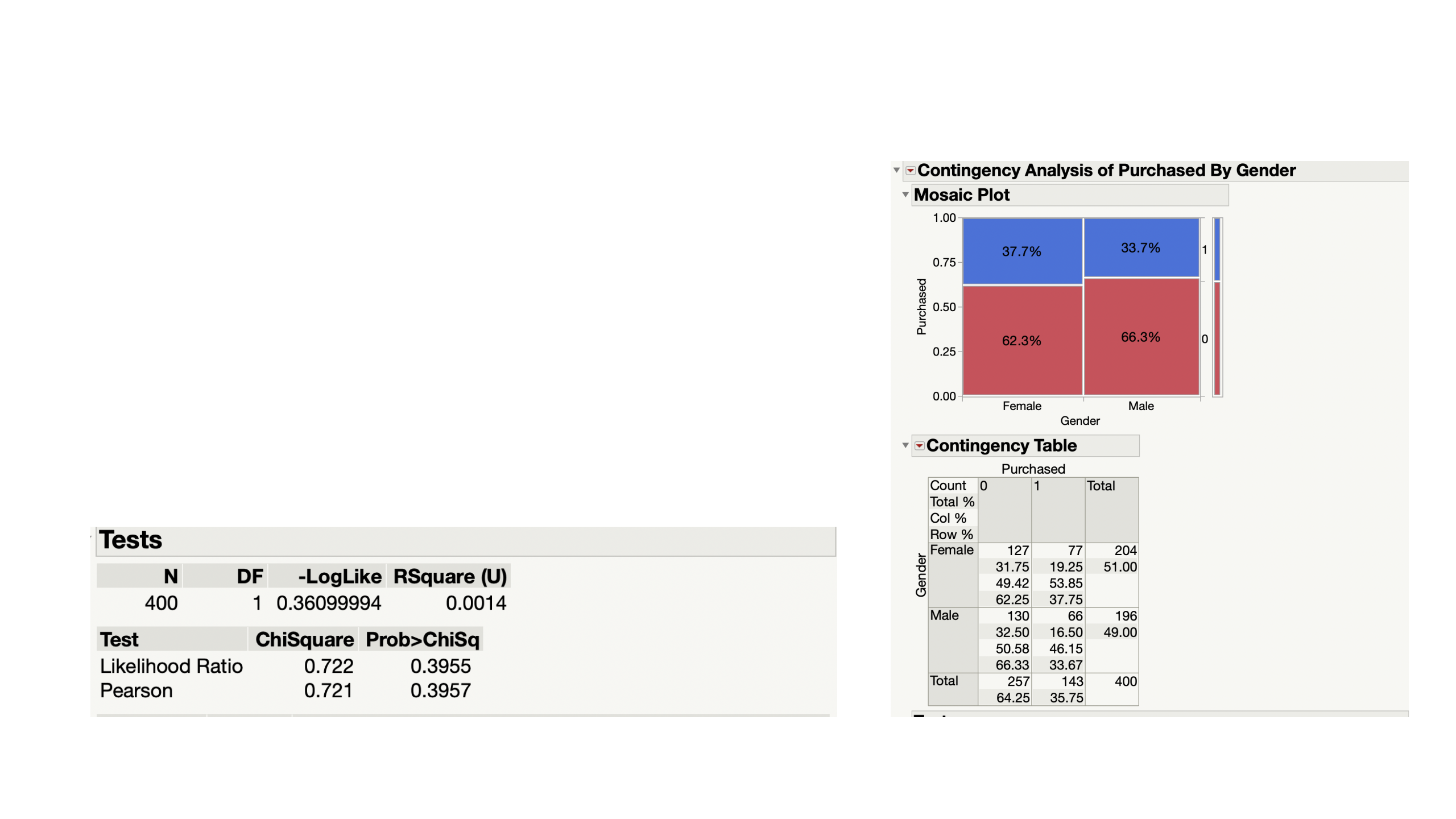
JMP (Inferential analysis): Simple Logistic
Regression
•Analyze -> Fit Y by X
•Y is binary and X is a categorical variable
•Data: Social_Network_Ads.jmp
3/7/21 12Dr. Asish Satpathy
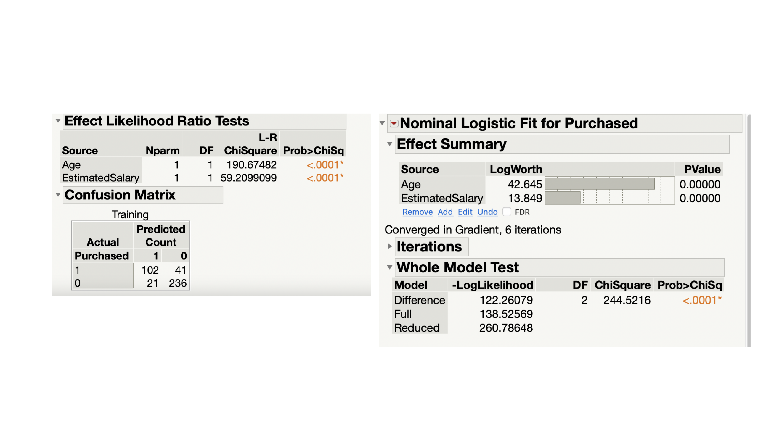
JMP (Inferential analysis): Multiple Logistic
Regression
Data: Social_Network_Ads.jmp
3/7/21 13Dr. Asish Satpathy

Regression Analysis Check list
•Check Analysis of Variance Table (Whole Model effect)
•Check R2 / Adjusted R2(Coefficient of determination) [Not important
for logistic regression]
•Check Residual plot [not important for logistic reg]
•Check Parameter estimate tables
•Check VIF for multicollinearity effect (only for multiple linear
regression)
•Model Equation / Model evaluation (Confusion matrix)
•Interpretations of your results
3/7/21 14Dr. Asish Satpathy

