Against Bayesianism and Corrections to Bayesianism

Two interrelated paradigms — subjective Bayesianism and Humean decision

theory — have had notable success as both prescriptive and descriptive

accounts of reasoning and rational decision-making. Subjective Bayesianism, as

pioneered by Bruno de Finetti and Frank Ramsey in the early 20th century, says

that partial beliefs can be represented by subjective probabilities, or credences:

real numbers between 0 and 1 that measure an agent’s subjective degree of

belief in a proposition. Subjective expected utility theory, as developed by John

von Neumann, Oskar Morgenstern, and L. J. Savage in the post-war period,

extends this to decision-making by positing utilities: real numbers measuring

the desirability of an outcome to an agent, such that rational decision-making

can be characterized as the maximization of the expected value of utility, relative

to the probability distribution given by the agent’s credences. In both cases, the

primary normative constraint on agents is internal consistency: credences must

obey the axioms of probability, and the construction that produces the utility

function assumes that the agent’s decisions conform to certain axioms of

consistency (such as transitivity of preferences).

A subsequent genre of philosophical work within these paradigms

acknowledges that the basic theories suffer from certain limitations or

unexplained paradoxes, then seeks to modify them so as to remedy the defect. In

some cases, these revisions appear to generalize the original framework; an

example is Ha´jek’s suggestion that the proper primitive notion for subjective

Bayesianism is not probability simpliciter, but conditional probability. In other

cases, the theory has the form of a “second-order” correction to the original

theory, such as the Principal Principle, which modifies subjective Bayesianism by

asserting a norm of correspondence to a feature of objective reality (physical

chance) under certain circumstances.

Some of the motivating cases for these revisions are persuasive to me and

some are not. But the data that really interest me are not atypical paradoxes, but

rather the ways in which the theories fail to describe our ordinary reality — the

everyday activities of reasoning and decision-making. If decision theory does, in

fact, provide a comprehensive account of rational decision-making, what

explains the difficulties in applying it to a job search? If Bayesian confirmation

theory accurately describes the convergence of agents to a shared conception of

the truth — if it is really a matter of eliciting priors and then bringing a shared

stream of evidence to bear on them — what explains continued resistance to

scientific consensus on questions of incredible importance?

The purpose of this work is to argue both against the original, “pure”

paradigms and against certain attempts to correct them. There is no single

underlying ground for these critiques. In some cases, I will defend the original

paradigm against the proposed correction. In others, I will argue that it is

nomologically impossible for agents in our universe to achieve the paradigmatic

ideal of rationality — due to constraints posed by mathematical and physical

limits — then argue that relaxing the paradigm to allow for bounded rationality

sacrifices the advantages that made the original thesis so philosophically

compelling. In a final group of cases, I will argue that the paradigmatic ideal of

rationality lacks normative force even for idealized, unconstrained agents. The

case being developed is for a wide net: an eclectic pluralism about the

representation of knowledge and about rational decisionmaking, one that

embraces both Bayesian and non-Bayesian foundational approaches rather than

trying to corral everything into a single framework. While the bulk of the

argument is negative, I will develop a positive proposal: a pluralist account of

probability that seeks to integrate both the frequentist and Bayesian

interpretations.

I am also including some work on the philosophy of set theory. This work is

thematically connected only inasmuch as I perceive Cantorian set theory as

setting a benchmark for formal methods in philosophy in general: in its

comprehensive illumination of the practice of mathematics, it shows us a level to

which other formal projects can aspire.

Chapter 2

Against Binding

Abstract

Binding is advocated as a correction to standard Humean decision theory for

three reasons: to allow an agent to behave consistently across anticipated shifts

in preferences, to resolve paradoxes in infinite decision problems, and to resolve

Newcomblike paradoxes. I argue that binding should not be seen as a single,

unifying solution to these problems. With regard to the first issue, I claim that

once we have properly distinguished shifts in preferences from akrasia, the

effect of binding is inherently to resolve conflicts in values, and to privilege one

set of values over another; thus, the binding agent cannot claim to be Humean.

With regard to infinite decision problems, I argue that there is an essential and

unavoidable breakdown of decision-theoretic concepts and methods in the

infinite setting, and that we should not be too concerned about this because of

the nomological impossibility of the problems. Finally, I argue that binding

(specifically, causal decision theory augmented with binding) provides the

correct answer in all Newcomblike problems, but that this is an essentially

different sense of the term.

2.1 Introduction

A Humean decision theory is one in which consistency is the only norm on

preferences. The modern paradigm is probably the expected utility theory of

Savage [1972]. Savage gives a formal setting that models decision-making under

uncertainty and states some intuitively acceptable axioms that should

normatively govern such decision-making. He then proves a representation

theorem stating that for any agent conforming to the axioms, we can construct a

probability distribution and utility function such that their actions maximize

expected utility over the distribution. Under a Humean interpretation of the

Savage axioms, these two free parameters — the subjective probability

distribution and the utility function — cover exactly the space of possibilities for

normative rationality, at least within the domain of applicability of the axioms.

All Kolmogorov-consistent probability distributions and all utility functions are

equally rational.

There are several settings for decision-making under uncertainty that seem

to fall outside the domain of applicability of the Savage axioms. For one, the

Savage axioms define a synchronic notion of rationality, and do not naturally

address questions about how an agent should behave in the face of preference

changes across time. They also explicitly exclude the possibility of modeling

certain kinds of infinite decision problems. Finally, they cannot model

“Newcomblike” problems in which the state of the world, concerning which the

agent is uncertain, cannot be separated from the agent’s actions.

A concept called binding has been advanced as a conceptually unified

correction to decision theory that covers all of these cases. Loosely speaking,

binding is the ability of an agent to commit in advance to a course of action, then

carry it out even if it is no longer preferred or recommended in the way it was

originally. My claim is that binding should not be viewed as a single concept that

unproblematically extends Humean decision theory into all of these domains. In

the diachronic preference change setting, I argue that binding is inherently non-

Humean, and furthermore that it is the wrong analysis of its motivating cases. In

the infinite setting, I argue that its role is to cover up a far-reaching breakdown

of decision-theoretic concepts, one that we should not be concerned about

because there is a deep contradiction between the cases and the nature of our

physical universe. Finally, in the Newcomblike setting, I think binding

(specifically, causal decision theory with binding) is in fact the correct response

to all Newcomblike cases — but I think the sense of binding relevant there is

essentially different from the ones invoked elsewhere.

2.2 Binding and diachronic preference change

The problem

The following scenario (“Diet”) is adapted from McClennen [1997]:

It is 6 AM and Joe wishes to begin a new diet, one that must be

followed strictly (i.e., there are no health benefits from partial

adherence to the diet). He has two choices: he can purchase a day’s

worth of perishable diet food and eat half of it for breakfast, or he

can eat a free meal of non-diet food. Because he wishes to diet, Joe

prefers the first option. But Joe also knows that if he diets now, then

at noon, he will face the choice between eating his remaining diet

food and eating a free non-diet meal, and his food cravings will cause

him to prefer the second of these options.

This scenario is sufficient to distinguish the three main alternatives with

respect to diachronic preference change. The naive or myopic choice is for Joe to

purchase the diet food at 6 AM and eat it, then break his diet at noon, at which

point he has neither his money nor the health benefits from dieting. How can he

avoid this outcome? The resolute choice is for him to buy the diet food and

commit in advance to eating it at both 6 AM and noon — this binding decision

allows him to obtain the health benefits at the cost of the money. But the

sophisticated choice is for him to reason that he will inevitably defect from the

diet plan at noon, and therefore that he should eat the free meal at 6 AM as well;

this lets him keep the money, at the cost of the health benefits.

In passing, I should note that my decision to treat “binding” and “resolute

choice” as synonyms departs somewhat from the literature on preference shifts.

In particular, Buchak [2013] uses “resolute choice” in the sense just described,

but reserves “binding” to mean changing the decision problem by actually

removing the future choice (in “Diet”, this might mean Joe leaving his meal pass

at home in the morning). However, it seems to me that the distinction can be

neglected in the case of ideally rational agents, by the following argument: if a

resolute choice is indeed the ideally rational action, then an ideally rational

agent will make it and follow through on it, and there will be no need for her to

actually deny herself the possibility of taking the less-preferred option.

Therefore, for such an agent, “resolute choice” in this sense subsumes or

displaces “binding”. The distinction, then, is only relevant in more

psychologically realistic settings where the agent might be unable to follow

through on a resolute choice. Since my discussion will neglect psychological

considerations of this sort, I will also neglect the distinction (but I will return to

the question of coercing one’s future selves in section 2.2).

Now, it is important to distinguish the intended Humean framing of this

situation from akrasia, or the phenomenon of an agent acting against his better

judgment. To see that this isn’t akrasia, it suffices to notice that akrasia

paradigmatically exists in the synchronic case — at any given moment, Joe might

prefer to diet, but find himself weak-willed and unable to resist a non-diet meal.

But if we take the Humean premise of this scenario seriously, what is happening

is necessarily diachronic. At 6 AM, Joe has a valid preference to diet, but at noon,

his preferences have changed and he has an equally valid preference to deviate

from the diet.

Does binding help?

At first glance, the intuition is clear that resolute and sophisticated choice are

helpful to an agent. After all, they provide the agent with additional decision-

making tools — surely that can’t be a bad thing! But this doesn’t survive scrutiny,

for just as we can construct cases where resolute choice is intuitively helpful, we

can also construct cases where it is intuitively harmful. Call this scenario

“Remarriage”:

Sam is unable to accept his mother’s remarriage. Therefore, Sam

prefers not to have any contact with her. However, Sam knows that it

will soon be the holiday season, which will provoke intense emotions

in him, which will cause him to prefer contacting her, reconciling

with her, and accepting her decision. Sam therefore makes a resolute

choice not to contact his mother.

Intuitively, Sam is harmed by his ability to choose resolutely. And as for a

scenario where sophisticated choice intuitively harms the agent, we have this

already in “Diet” itself, where it causes Joe to abandon his diet before it even

begins.

There is a simple analysis of the intuitions here. In both scenarios, we intuit

that of the two conflicting preferences exhibited by the agent, one is superior in

the sense that it better reflects the agent’s true interests or values. Resolute

choice causes the agent to act according to the initial preferences, and

sophisticated choice causes him to act according to the subsequent preferences.

So if the initial preferences are inferior, resolute choice is harmful, and vice

versa. Now we have an apparent symmetry: resolute and sophisticated choice

can both help and harm. So what justifies them?

McClennen is aware of this difficulty and confronts it directly. For him, the

justifications for resolute and sophisticated choice are not rooted in their claims

to help. Rather, they are justified because they dominate myopic choice. If we

look back to “Diet”, the resolute chooser has his health and the sophisticated

chooser has his money, but the myopic chooser has neither — his diachronic

inconsistency gets him the worst of both worlds. So without taking a stance on

whether Joe’s initial or subsequent preferences are superior, we still have

grounds to say that myopic choice is irrational.

Nevertheless, I think this justification of binding also fails. The problem is

that this analysis does not properly distinguish binding, as a means of avoiding

myopic choice, from the sunk cost fallacy. Again, if we take the Humean premise

of “Diet” seriously, Joe’s preference to stop dieting at noon is an all-things-

considered preference — Joe has already accounted for his past desire to diet,

his ability to continue dieting at no additional expense, and all similar

considerations, and nonetheless prefers to eat the non-diet meal. It seems to me

that if Joe continues to diet despite this, he is behaving in a manner

indistinguishable from standard examples of the sunk cost fallacy, for example

“Movie”:

Dave values both money and time. A new two-hour movie has been

released, and he believes he will enjoy it sufficiently to justify

spending two hours to watch it and $10 for a ticket. After one hour,

Dave realizes that the movie is very bad and will not get any better,

so he has a higher expected utility from walking out of the movie and

saving the remaining hour than from finishing the movie.

Nevertheless, Dave stays until the end of the show, reasoning that

otherwise he will have wasted his investment of $10 and an hour of

time.

We understand Dave’s concern for his unrecoverable sunk costs as irrational.

But if the underlying motivation for Joe’s decision to keep dieting is merely to

avoid diachronic inconsistency (instantiated by the cost he has already paid for

the diet food), Joe seems to be committing the same fallacy. The difference

between Joe and Dave is that Joe actually anticipates that he will defect from his

initial plan. But when noon comes around and Joe actually experiences his all-

things considered preference to defect, why should the existence of this past

prediction make a difference? I claim that the only Humean-rational action for

him is to defect, and if he does not defect, it represents a non-Humean rejection

of his present preferences in favor of his past ones.

This gets at an asymmetry between resolute and sophisticated choice: unlike

its dual notion, sophisticated choice can still be understood as Humean. As a

sophisticated chooser, Joe can say, “My preference is to diet. But I see now that

since my future self will inevitably defect from the diet, it is therefore impossible

for me to realize my preference. So I’ll abandon the diet and save my money.”

Nothing about this is non-Humean — even if it seems perverse for Joe to reason

via backwards induction against his future self, Joe is not actually denying the

validity of any preferences.

I do not think this is a reason to endorse sophisticated choice over resolute

choice — it would be absurd to recommend that one should always defer to

one’s anticipated future preferences. Rather, I think that the Humean framing of

the problem is wrong. The correct analysis of “Diet” is that Joe’s initial

preference is good and his subsequent “preference” is akratic (vice versa in

“Remarriage”).

Natural notions of compromise?

Is there a natural way to perform preference reconciliation? One possibility is to

choose the preferences that one will hold for longer amounts of time, i.e., the

preferences acceptable to as many of one’s future time-slices as possible. This

accords with our intuitions in “Diet” and “Remarriage” — more of Joe’s future

selves will be happy if he completes the diet, and more of Sam’s future selves

will be happy if he reconciles with his mother. But I think this idea runs into

trouble quickly. Call this scenario “Lotus”:

Odysseus prefers to return home to Ithaka. But he is presently near

an island, on which grows the lotus. Anyone who eats the lotus

immediately ceases to prefer anything other than eating more lotus,

a preference which is guaranteed to be perfectly satisfied since the

supply of lotus is unlimited. In contrast, Odysseus knows that if he

returns to Ithaka, preference satisfaction among his future selves will

not be nearly so complete — he will inevitably have to deal with

marital disputes, bad weather, and all the other shortcomings of

quotidian life. Therefore Odysseus considers himself rationally

obligated to stop his journey and eat the lotus.

As Buchak (forthcoming) observes, there is a duality between personal

utility theories and utilitarianisms — one’s probability-weighted future selves

are like differently sized segments of a population, and maximizing personal

expected utility is like maximizing utility across the population. Viewed in this

light, Odysseus’s lotus-eating future self is a “utility monster” in the sense of

Nozick [1974], an entity that tyrannizes its fellows in any compromise by virtue

of its superior ability to experience preference satisfaction.

A similar problem attaches to the suggestion in Gauthier [1997] that there

are situations where some additional structure on the preferences tells us which

to follow. Specifically, Gauthier distinguishes between “proximate” preferences

(loosely speaking, near-term preferences experienced when confronted with a

decision) and “vanishing-point” preferences (again loosely, long-term

preferences held by the majority of one’s future selves), and suggests that

resolute choice is a way for us to act on our vanishing-point preferences when

they conflict with proximate preferences. I think that there are many cases in

which an agent’s vanishingpoint preferences are superior to their proximate

preferences, but I don’t think this is a generally valid prescription for preference

reconciliation (nor, I think, is Gauthier claiming this), and again I don’t think

resolute choice is the right way to model the phenomenon. Rather, such an agent

should reason that their proximate preferences are akratic because their

vanishing-point preferences reflect their true underlying values.

What is the right analysis of “Lotus”? Odysseus doesn’t see the preferences of

his lotuseating self as equally valid with his current preferences. But there is a

disanalogy with the previous cases because the lotus eater does not necessarily

seem akratic. Rather, Odysseus seems to have an underlying system of values

that deems the preferences of his current self praiseworthy and the preferences

of the lotus-eaters blameworthy. The diagnosis of akrasia does not exhaust the

possibilities for non-Humean preference reconciliation; we see from this that

there are also resolutions that refer to ethics. This is related to the argument of

Paul [2015] that when making decisions that will result in personal

transformations of sufficient magnitude (in particular, whether to have a child),

we cannot simply adjudicate among the possibilities by reflecting on our

phenomenal preferences (i.e., by thinking about what the results of our decisions

would “feel like”), because phenomenal experiences are incomparable across the

transformation. In such cases, ethics may be the only way to reconcile the

preferences.

Preference shifts on neutral ground

But what if neither akrasia judgments nor ethics intervene to reconcile the

preferences? In the absence of any considerations that might transcend

preference satisfaction, I think the non-Humean can acknowledge that

preference satisfaction is itself a good, and that a choice can be the best one

merely in virtue of offering more satisfaction to more of the agent’s time-slices.

Consider “Lilliput”:

Skyresh is an ambitious young citizen of Lilliput, about to enter

university, after which he intends to pursue a career in public

service. In the highly partisan society of Lilliput, official preferment

may be obtained either through allegiance to the Big-Endian Party or

the Little-Endian Party; the two parties are indistinguishable, except

for their views on the end at which to break a soft-boiled egg. Right

now, Skyresh strongly prefers the Big-Endian Party. However, he is

aware that his university is dominated by Little-Endians, and he

predicts that under the influence of their ideas, by graduation he will

prefer them instead. Skyresh is now faced with the option of

irrevocably declaring his allegiance by praising the Big-Endians in an

editorial for his local paper (which will live on indefinitely in

Internet search results, dooming any chance of finding favor with the

Little-Endians).

Skyresh has the ability to bind himself to Little-Endianism. Should he use it? I

think it’s clear that he shouldn’t. Inasmuch as the decision for one party over the

other plausibly impacts only the preference satisfaction of his future self,

without any ethical or normative implications, it seems like his present self has

no business intervening and imposing a preference. Perhaps this constitutes a

very qualified endorsement, ceteris paribus, of sophisticated choice.

Time-slice rationality and the Sure-Thing Principle

The conclusion I drew from “Movie” — that consistency, in itself, is not a reason

to suppress a current preference that conflicts with a past one — amounts to an

endorsement, at least within the domain of preference shifts, of time-slice

rationality, which rejects the idea of inherently diachronic norms of rationality.

At first blush, the time-slice view may seem like an alarming concession in that it

denies the force of diachronic inconsistency arguments (such as the Dutch Book-

type arguments against violations of conditionalization). But this doesn’t imply

wholesale bullet-biting with respect to all such arguments; rather, the claim is

that if there is a failure of rationality, it must in fact be synchronic. Joe’s defection

from his diet can indeed be judged irrational, but its irrationality is exactly

synchronic akrasia, the same phenomenon that might synchronically prevent

him from acting on his preference to diet.

However, this conclusion is prima facie in tension with my view on a related

topic, namely, the rationality of ambiguity aversion and the Ellsberg preferences.

This is the classic case of Ellsberg [1961]:

An urn contains 90 balls. 30 are red, and the remaining 60 are black or

yellow in some unknown proportions. You are offered a choice between

two bets, I and J: bet I pays $100 if you draw a red ball, and bet J pays

$100 if you draw a black ball. You are then offered a second choice

between two bets (on a separate i.i.d. draw from the same urn), X and Y:

bet X pays $100 if you draw a red or yellow ball, and bet Y pays $100 if

you draw a black or yellow ball.

As Ellsberg observed, it is inconsistent with the axioms of expected utility

maximization to strictly prefer I to J, but also strictly prefer Y to X, i.e., to prefer

the bets with known objective probabilities. To see this, observe that without

loss of generality, the agent values

$100 at 100 utiles. Then, fix any credences in P(B) and P(Y ) satisfying

. Then E[I] < E[J] implies P(R) · 100 < P(B) · 100 and P(R) <

P(B). This in turn implies that E[X] = P(R) · 100 + P(Y ) · 100 < P(B) · 100 + P(Y ) ·

100 = E[Y ].

Given Savage’s representation theorem, any failure to maximize expected

utility can be redescribed as a violation of one of Savage’s axioms of rationality.

And in this case, the axiom violated is the “Sure-Thing Principle”, which states

that when two gambles share a “subgamble”, one’s preference between those

gambles must be determined by one’s preference between the remaining non-

shared components of the gambles. In this case, X and Y share a payoff of $100

on yellow; when this is removed, the remaining components of the gamble are

exactly I and J respectively. Therefore, one who accepts the Sure-Thing Principle

and prefers I to J must also prefer X to Y.

The Ellsberg preferences have inspired a rich literature on how to

“rationalize” them, i.e., propose a more lenient notion of rationality that is

compatible with them. But AlNajjar and Weinstein [2009] oppose this program

and argue that the preferences are in fact irrational, because the violation of the

Sure-Thing Principle gives rise to diachronic Dutch Books. The general form of

their Dutch Book cases is as follows: Initially, the agent chooses between bets X

and Y (so an agent with the Ellsberg preferences will choose Y). Then, the ball is

drawn and it is announced whether it is yellow. If it is, the agent receives the

$100 payoff and the game is over, but if not, the remaining subgambles (now

that yellow has been excluded) ostensibly coincide with I and J. The agent is then

offered the opportunity to switch subgambles; the Ellsberg agent, who is now

committed to J, will allegedly seek to switch to I.

This appears to be a diachronic preference shift analogous to the one in

“Diet”. And therefore, the scenario admits of similar perturbations: one may add

penalties at different stages of the problem such that the agent’s choices are

strictly dominated by another set of choices, or otherwise appear unattractive.

In the Humean framework of Al-Najjar and Weinstein, the relevant criterion is

one of “regret” or “embarrassment”; when confronted with the suboptimality of

their diachronic choices, the agent should be moved through introspection to

reconsider their synchronic preferences as well.

The clearest example is “naive choice”, which corresponds to the following

variant of the scenario: the agent is required to pay an initial penalty of ϵto

choose Y over X, then allowed to switch from J to I with no penalty in the case

where the ball is not yellow. The agent consequently receives $100 - ϵon yellow

and $100 - ϵon red; these choices are strictly dominated by an initial decision to

choose X without switching, which pays $100 on yellow and $100 on red. I

concur with the authors that this represents a failure of rationality. The authors

then consider “sophisticated choice” as an alternative, in which the agent

chooses X over Y initially and then refuses to switch; they concede that this

strategy avoids choosing any strictly dominated options, but argue that it leads

to new paradoxes. Even though I am skeptical of the specific arguments they

make, I also find sophisticated choice unattractive as a response.

Here is where non-Humeanism can be put to work: the non-Humean should

not be concerned with avoiding embarrassment per se, but should rather seek

the right answer to the case — which one may then hope will not be too

embarrassing. (Heuristically, one might say that embarrassment will typically

constitute defeasible evidence that an answer is wrong — but if the right answer

turns out to be embarrassing, so be it!) And it seems to me, for reasons I will

elaborate elsewhere but which are rooted in frequentism, that the right answer

in this case is to choose Y initially and then refuse to switch. Now, this appears to

involve an act of resolute choice or binding, and therefore to clash with the

arguments I have just given against binding as a response to preference shifts. In

fact, Al-Najjar and Weinstein [2009] give a different perturbation of the scenario

in which this answer appears to entail the commission of the sunk cost fallacy.

What are the intuitions behind picking Y and sticking with it? First, the agent

with Ellsberg preferences prefers to receive payoffs in the event of black-or-

yellow, since this is the event with known objective probability; if he can be

manipulated into receiving a payoff on red-or-yellow instead, then it is likely

that something has gone wrong. But furthermore, any agent in this situation

(Ellsberg preferences or no) knows that if yellow balls are scarce, then black

balls must be plentiful. And if yellow balls are scarce, the agent who switches is

that much more likely to hear the announcement that the drawn ball is not

yellow and therefore to cheat himself out of benefiting from the plenitude of the

black balls. (In the worst-case scenario, there are 0 yellow balls and 60 black

balls, and the switching strategy wins with probability only .) This suggests that

the announcement that the ball was not yellow may potentially constitute

evidence that it is black rather than red — although the precise nature and value

of the evidence need to be clarified.

However, this is already enough to see that the subgamble structure alleged

by Al-Najjar and Weinstein [2009] is invalid — and that this problematizes their

arguments against the rationality of the synchronic Ellsberg preferences. The

agent who has initially chosen X or Y and then has been told that a single draw

from the urn produced a non-yellow ball is not, in fact, in the same epistemic

position as an agent faced with the choice between I and J. This is so even for a

Savage-normative, fully Bayesian agent. Consider in particular the agent who

begins with the uniform prior over proportions of black and yellow balls, i.e.,

assigns probability to each hypothesis Hi that the number of yellow balls is i,

for 0 ≤ i ≤ 60. This agent initially has credences and

is therefore indifferent beween X and Y. But upon hearing that a non-yellow ball

was drawn, she will update her credence in P(Hi) to:

(2.1)

This shifts probability mass away from Hi where i is high, and towards Hi

where i is low — the announcement that the ball is not yellow is informative not

merely about the ball, but about the composition of the urn. Now, our Bayesian

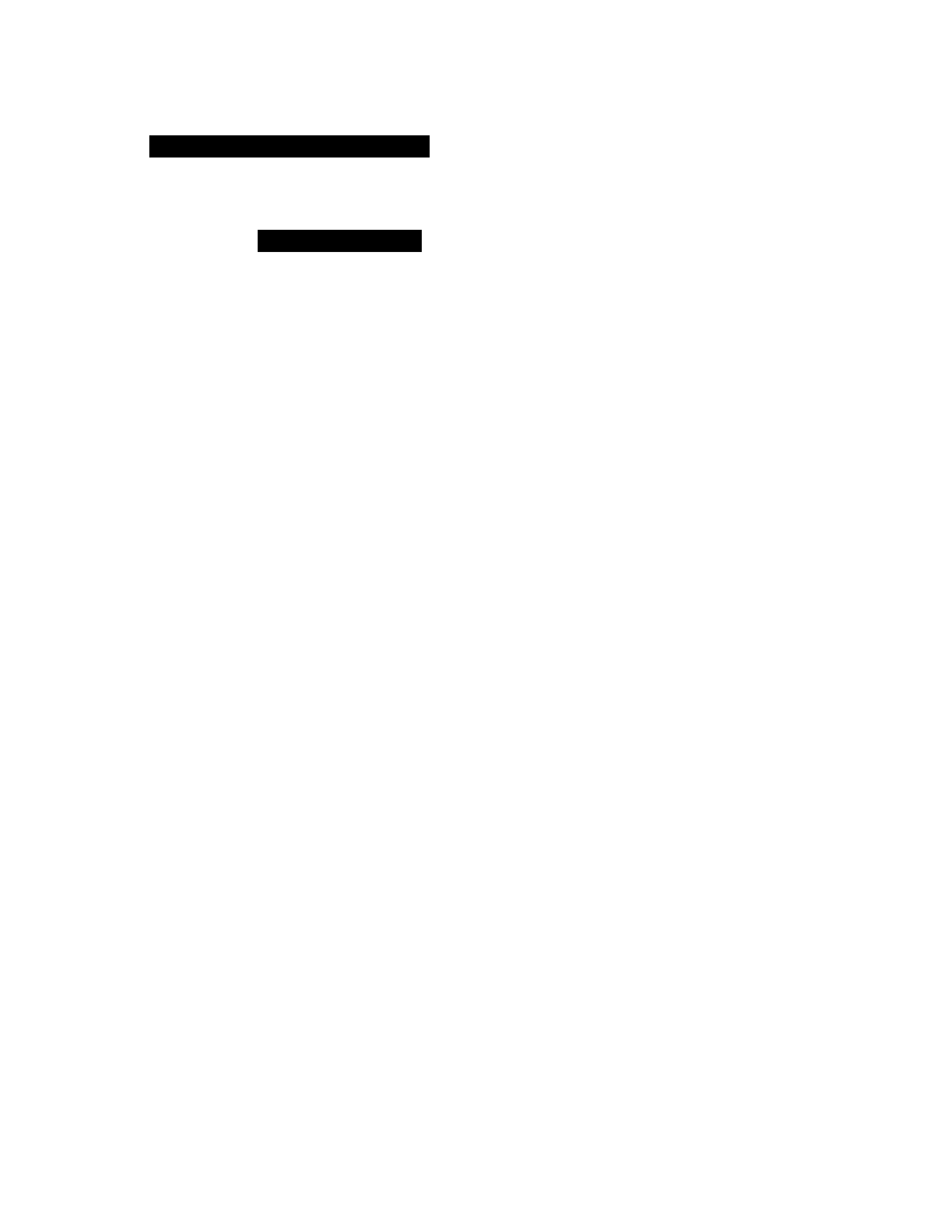
agent will also update her credences in R and B by simple conditionalization —

¬Y ) = P ′(B) — and will therefore remain indifferent between I and J,

experiencing no shift in preferences concerning bets on the currently drawn ball.

(In contrast, her beliefs about the next ball drawn with replacement from the

same urn are

.39,P ′(Y ) ≈ .27.) But it is certainly conceivable that a non-Bayesian agent could

update his beliefs not merely about the urn, but about the currently drawn ball,

in a way such that black is more “likely” than it was before the announcement.

Indeed, to assert that this is irrational (by insisting that the agent’s preferences

after the announcement must coincide with their preference between I and J in

the synchronic Ellsberg case) seems to presuppose that Bayesian

conditionalization is normative for belief update, and therefore to beg the

question against non-Bayesian epistemologies.

I have argued that strictly speaking, one’s preference between I and J does

not commit one to a preference at the second time-step in the diachronic

Ellsberg cases. But nonetheless, my view does in fact entail something like a

preference reversal, so it behooves me to examine in detail the diachronic case

Al-Najjar and Weinstein bring against it:

Consider an urn as in the original Ellsberg case. Initially, you are

offered a bet that pays $100 on a draw of yellow, in exchange for

some fixed cost s. Once you have made your decision, the ball is

drawn and it is announced whether it is yellow. If it is yellow, you

receive $100 if you paid s and nothing otherwise. If it is not yellow,

you are offered a choice between a bet that pays $100 on red and a

bet that pays $100 on black, both at no cost.

Now by dominance, any agent should consider the initial bet worthwhile at s

= 0 and not worthwhile at s = 100; by continuity, the agent must have some

indifference price 0 ≤ s <¯ 100 for the bet. Suppose an agent with the Ellsberg

preferences is first offered the bet for a price lower than ¯s; the authors argue

that this agent will buy the bet, then choose the payoff on black if it fails (i.e.,

choose Y minus the penalty s). But if the bet is offered instead for a price higher

than ¯s, the agent will refuse the bet, then choose the payoff on red (i.e., choose

I). Al-Najjar and Weinstein then claim that this is an instance of the sunk cost

fallacy: the agent’s preference between black and red appears to depend on

whether he has paid for the bet on yellow, but any such cost is sunk at the time

of the choice.

Again, I think it is not a necessary consequence of the Ellsberg preferences

that an agent exhibit this behavior in the diachronic case. But I will affirm the

rationality of agents that exhibit this apparent sensitivity to sunk cost. In

particular, consider the following simplified model: Ezra, a frequentist, seeks to

maximize long-run winnings by buying bets with positive expected value in

money according to known objective probabilities. In the diachronic scenario,

Ezra therefore values “red” at 100 and the package of “yellow or black” at

100; his ¯s is the difference between those two values, . Faced with an initial

offer of s = 40, he rejects it and chooses red. But with an offer of s = 20, he

accepts and then chooses black if it fails.

Once yellow has failed to come up, why doesn’t Ezra want to switch to red? I

will sketch an explanation now (I hope to give a full account later as part of a

general theory of iterated betting games). Recall that Ezra is modeling this bet as

one in a series, and his success criterion depends on performance over the

entire series. But at the same time, Ezra must imagine that for every bet in the

series, just like for this one, he will be in a state of non-Bayesian uncertainty as

to the proportions of black and yellow balls. That is to say, he imagines that

every draw in the series will be from a fresh urn, with an unknown proportion of

balls, For reasons related to the reference class problem, Ezra is imagining that

he cannot learn anything about the proportions across distinct draws in the

series — so he must use a memoryless strategy for betting. And the memoryless

strategy that switches to red every time wins, in the worst case (where the

proportion of yellow balls is always ), with probability only , whereas the

strategy that sticks with black wins with guaranteed probability .

There are two lessons here. First, note that if Ezra is told that a single

previous draw from the urn was not yellow, and then has to choose between

black and red on a fresh draw with replacement from the urn, he will still choose

red — in contrast to his behavior in the diachronic scenario, where he sticks

with black. It follows that his preferences, specifically his refusal to switch,

necessarily commit him to time-worm as opposed to time-slice rationality.This

is somewhat surprising but on closer inspection it is quite natural: long-run

frequency is inherently a diachronic notion, so achieving goals defined in terms

of long-run frequency requires a diachronic notion of rationality.

The other is that the concept of sunk cost, as it appears in the economics

literature, appears to be so broad as to presuppose time-slice rationality. In

regard to cases like “Movie”, I affirm that it is possible to commit the sunk cost

fallacy. But although Ezra’s preferences have a whiff of the paradoxical about

them, they seem to stand up to reflective scrutiny: if they are embarrassing, they

are only embarrassing by association. It therefore falls to advocates of time-

worm rationality to formulate a new definition of the sunk cost fallacy that

distinguishes the two cases. My intuition is that what Dave is doing in “Movie”

(and Ezra is not doing in the diachronic Ellsberg case) is “throwing good money

after bad” — expending new resources in pursuit of an objective that no longer

makes sense. But it is beyond the scope of the present discussion to make this

rigorous.

Similarly, I am unable to formulate a definitive response to the Allais paradox

based on these principles. My intuition is that the Allais preferences (which, like

the Ellsberg preferences, involve a violation of the Sure-Thing Principle) are

rational. But there is a similar diachronic Dutch Book against the Allais

preferences, and it is more persuasive to me than the one against the Ellsberg

preferences. I leave the matter here.

2.3 Infinite decision problems

Continuing the theme of binding as an correction to standard decision theory,

Arntzenius et al. [2004] propose binding as a solution not to diachronic

preference change, but to dilemmas that arise in the context of so-called infinite

decisions — for the purposes of their discussion, decision problems where the

scenario includes an at least countably infinite number of (possibly diachronic)

choices. They give six such scenarios, then argue that all are in principle

isomorphic to a proposed ur-scenario called “Satan’s Apple”. Finally, they

propose binding as the common solution to all the scenarios. To the skeptic who

would prefer to exclude infinite decisions from consideration, they offer this

challenge:

For we are loath to constrain the scope of decision theory with such

seemingly ad hoc bans. And we would be unsatisfied with a

resolution of the puzzles that did not reflect their common character.

Accordingly, my reply is two-pronged. First, I will dispute the commonality of

the cases — I will attempt to dismiss three of the six cases as fallacious in ways

that are orthogonal to the question of infinite decisions. But I accept their

analysis of the other three as variants on the same prototypical “Satan’s Apple”

problem. I will then reject the normative implications of this problem for

decision theory, based on the idea of nomological possibility that Shieber [2014]

invokes in the context of the Chinese Room argument. In brief, there is a deep

contradiction between infinite decision problems and the nature of the physical

world we live in; since this is the world that Bayesian decision theory attempts

to model, the refusal to consider them cannot be considered an “ad hoc ban”.

Decision agglomeration and the converse Dutch Book theorem

The core issue at stake in the six scenarios is the “agglomeration” of individual

decisions into packages. It is therefore useful to review the converse Dutch Book

theorem, which provides some guarantees relating the favorability of a package

of bets to the favorability of the individual bets:

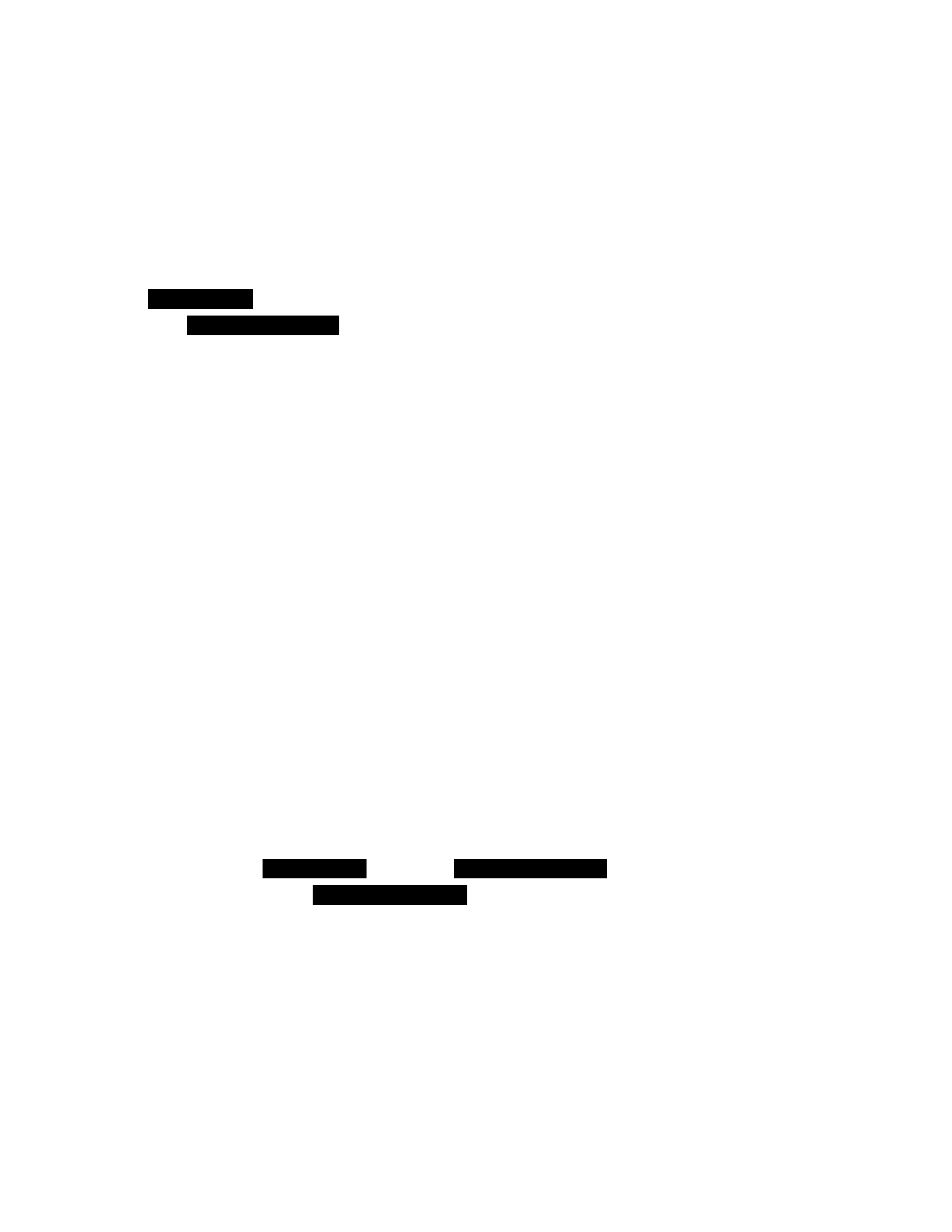
Theorem 1 (Linearity of expectation). Let X and Y be random variables, and a ∈

R. Then: 1. For any random variable X and constant a, E[aX] = aE[x].

2. For any random variables X, Y , E[X +Y ] = E[X]+E[Y ]. (Note that X and Y need

not be independent.)

Corollary 1. Let X1 ...Xn be any finite sequence of random variables, and let

Then .

Corollary 2 (Converse Dutch Book Theorem). Assume an agent bets

(unconditionally or conditionally) according to the betting prices given by a

consistent subjective probability distribution P. Then there is no finite package of

bets this agent will accept that results in a sure loss (i.e., the agent is not vulnerable

to finite Dutch Books).

Proof. Let c(B) denote the cost of a bet and w(B) its payoff. For an agent to

buy an unconditional bet B on X, it is necessary and sufficient that c(B) ≤

P(X)w(B), equivalently that E[B] ≥ 0. For a conditional bet B on X given Y , it is

necessary and sufficient that c(B) ≤ P(X | Y )w(B), which is equivalent to E[B | Y ]

≥ 0, and since E[B | ¬Y ] = 0 and E[B] = P(Y )E[B | Y ] + P(¬Y )E[B | ¬Y ] this is

again equivalent to E[B] ≥ 0.

Therefore, any bet the agent will buy has nonnegative expected value. Thus,

by linearity, any package consisting of positive real-valued quantities of finitely

many of these bets must also have nonnegative expected value. However, every

outcome of a Dutch Book has negative value, so the expected value of a Dutch

Book is negative — therefore such a package cannot be a Dutch Book. □

The problem is that this result is very nearly sharp. In particular, the package

of bets cannot in general be infinite:

Theorem 2. Expectation need not be countably additive, i.e., there exist random

variables

X1,X2,X3 ..., with , such that . (A sufficient condition

for equality to hold is

A particularly elegant counterexample is Vann McGee’s “airtight Dutch Book”,

which Arntzenius et al. [2004] reproduce as scenario #3 (“Trouble in St.

Petersburg”). The counterexample takes the form of an infinite package of bets

on the outcome of a geometric random variable X with p = 0.5, i.e., the number of

times one has to toss a fair coin before it lands heads. Bet B1 loses $1 if the coin

never lands heads, and wins $3 if it lands heads on the first toss. Then bet B2

loses $4 if the bet lands heads on the first toss, but wins $9 if it lands heads on

the second toss; bet B3 loses $10 if it lands heads on the second toss, but wins

$21 if it lands heads on the third. The bets continue in this pattern such that if

the coin lands heads on the nth toss, bet Bn wins $x dollars but Bn+1 loses $(x+1)

dollars. Thus, although each bet has positive expected value, the package leads

to a sure loss of $1.

Now, Arntzenius et al. observe that probability and expected value can be

eliminated from this scenario without changing its essence. Here is their

proposed ur-scenario, called “Satan’s apple”:

Satan has cut an apple into a countably infinite number of pieces,

labeled p0,p1,p2 .... If Eve takes infinitely many pieces, she will be expelled

from the Garden; any outcome in which she is expelled is worse than

any outcome in which she is not. However, for any piece pt, Eve (ceteris

paribus) prefers having the piece to not having it. During a countably

infinite sequence of time-steps, at time step t Satan offers Eve the option

of taking piece pt. At each such time-step, Eve reasons that taking the

piece does not imply that she will be expelled. Moreover, whether or not

she is ultimately expelled, she prefers to have the piece; therefore,

taking pt dominates not taking it. Eve consequently takes every piece

and is expelled from the Garden.

What are we to make of this? For Arntzenius et al., binding is an ability that

agents may or may not possess. If Eve is able to bind, then at the outset of the

scenario, she should bind to a course of action where she takes some finite

number of pieces and then stops. But if Eve is unable to bind, then (at least

under some additional assumptions about her decision-making process) the

outcome of expulsion is inevitable, indeed an obligation of rationality. On their

view, infinite decision problems like “Satan’s apple” demonstrate the usefulness

of binding; conversely, if an agent is unable to bind, then the agent’s failure on

“Satan’s apple” is not a failure of rationality, but merely reflects their lack of

capabilities.

I agree with the authors that “Satan’s apple” represents a paradigmatic

breakdown of decision agglomeration in the infinite setting — that is to say, it

exemplifies a phenomenon where an infinite number of optimal decisions form

a suboptimal package. However, their case for binding as a unifying framework

for infinite decision problems rests on the identification of several prima facie

different scenarios as instances of “Satan’s apple”. Therefore, before disputing

the validity of “Satan’s apple” as a counterexample to finite decision theory

without binding, I will address some cases where I believe the identification

with “Satan’s apple” to be spurious.

The two-envelope paradox

The two-envelope paradox has many variants, but this is the basic form as given

by Broome

[1995]:

Alice shows Bob two envelopes, one blue and one red. Each envelope

contains a check for a nonzero amount of money, and the amount on

one of the checks is twice the amount on the other, but Bob doesn’t

know which check is where. Initially, Alice gives Bob the blue

envelope. She then offers him the opportunity to switch to the red

envelope. Bob is an expected value maximizer and reasons as

follows:

let B be the amount of money in the blue envelope. Then, with

probability , the red envelope contains , and with probability , it

contains 2B, so the expected value of the red envelope is

, which is strictly greater. Accordingly, Bob

switches envelopes. Alice then offers him the opportunity to switch

back, and he reasons similarly that if the amount in the red envelope

R, the expected value of the red envelope is ,

which again is strictly greater. Following these rationales, Bob

switches indefinitely between the two envelopes.

Now, Arntzenius et al. [2004] suggest that in at least one version of the

problem, an agent with the ability to bind should resolve the paradox by binding

to stay with the blue envelope. But as a solution to preference cycles, binding

seems perverse — surely the problem must be that at least one of the links in

the cycle is fallacious! My view is that the various versions of the paradox rest on

subtle ambiguities in the formulation and abuses of the probabilistic formalism;

when the problem is sufficiently clarified and the reasoning is corrected, the

paradox always disappears.

The main issue with the original formulation is that Bob is reasoning about B

and R as though they were random variables, in particular taking their

expectation, even though no distribution has been specified for them. Let us

begin by assuming that B and R are drawn from some joint distribution D(B,R)

satisfying the constraint “B > 0, and either B = 2R or R = 2B”. For now, let’s also

assume that the expectations E[B] and E[R] under this distribution are finite.

Now, if Bob’s credences about the values are captured by a particular

distribution D — either because they are his priors, or perhaps because they

have been announced to him as the terms of a lottery — then the paradox

immediately disappears. Bob should value each envelope according to its real-

valued expectation, and should switch to the envelope with the higher

expectation.

Bob might wish instead to formulate a course of action valid for any possible

distribution D. A useful comparison is with the “largest number” puzzle of Cover

[1987]: Alice picks two distinct numbers l < h in R, then flips a fair coin and

reveals l on tails and h on heads. Bob must then guess whether the revealed

number is l or h. Cover describes a probabilistic strategy for Bob such that for

any distribution D(l,h) that Alice draws the numbers from, there exists > ϵ0

such that Bob guesses correctly with probability Ideally, we would be able

to derive one of these three results: either (a) for any such distribution, E[B] <

E[R] (so Bob should switch), (b) for any such distribution, E[B] = E[R] (so Bob

should stay), or (c) for any such distribution, E[B] > E[R] (so Bob should stay).

That is to say, one might hope that either the apparent symmetry of the problem

gives rise to an argument that the envelopes are equivalent, or that Bob’s

informal argument for switching in one direction can be made rigorous. But this

is trivially impossible. Consider D1, which assigns probability 1 to B = 1,R = 2,

and D2, which assigns probability 1 to B = 2,R = 1. Then, under D1, E[B] < E[R],

and under D2, E[B] > E[R].

However, we can derive conflicting versions of the desired relations by

placing additional, seemingly innocuous constraints on the structure of D. For

example:

1. Fix a distribution on B such that B > 0 and E[B] is finite. Produce D(B,R) by

sampling a value b from the distribution, setting B = b, then flipping a fair

coin and

9Bob samples a number g from a distribution supported over all of R, such as the standard

normal distribution. Let the revealed number be x; if x < g, Bob guesses that x is the lower

number, and if g ≤ x, Bob guesses that x is the higher number. In the event that g < l < h or l < h <

g, this strategy succeeds with probability . But if l < g < h, it succeeds with probability 1 — and

since the distribution was supported over all of R, the probability that l < g < h must be some >ϵ

0; the strategy therefore succeeds with probability .

setting R = 2b on heads and on tails. By linearity of expectations, the

expected value E[R] of the red envelope is ]. Bob

should switch to the red envelope and not switch back.

2. Fix a distribution on L such that L > 0 and E[L] is finite. Produce D(B,R) by

sampling a value l from the distribution, then flipping a fair coin and

setting B = 2l,R = l on heads and B = l,R = 2l on tails. Again by linearity of

expectations, the expected value of each envelope is now ]. Bob

should not switch envelopes.

So these assumptions lead to conflicting, but individually non-paradoxical,

recommendations. The problem is that neither of these techniques for

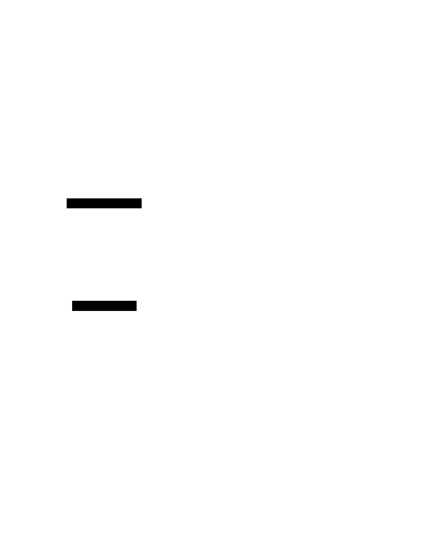
expanding a univariate distribution into the bivariate distribution D(B,R) is

“complete”, in the sense of being capable of generating all the possible bivariate

distributions. In particular, neither technique can generate the bivariate

distribution D1. It follows that in imposing the additional constraints, we have

put our thumb on the scale — it is implicit in constraint (1) that the red

envelope is better than the blue, and in (2) that they are equivalent. In the

original version of the problem, without such a constraint, the premises are too

weak to derive that any particular course of action is optimal. But even so, the

paradox disappears in the sense that it demonstrably does not follow from the

premises that Bob is rationally obligated to switch envelopes once, let alone

twice.

Finally, we must consider variants of the problem where E[B] and E[R] can be

infinite. Broome [1995] defines a specific distribution D(B,R) in the following

way: the value L of the smaller envelope is sampled from a distribution assigning

, for all n ∈N. Then the distribution is extended to a

bivariate distribution as in scenario (2) above. Broome shows that this

distribution has the following properties:

1. The unconditional expectations E[B] and E[R] are both infinite (alternately,

undefined).

2. For any value b of B, the conditional expectation E[R | B = b] is finite and

strictly greater than b. Specifically, E[R | b = 1] = 2, and for any b > 1, E[R | b

= b] =

. (So Bob, holding the blue envelope, might reason as follows:

if he

were allowed to open it and look at the value, no matter what value he saw,

he would expect the value in the red envelope to be even higher.)

3. For any value r of R, the conditional expectation E[B | R = r] is finite and

strictly greater than r. (That is to say, the analogous property holds for the

red envelope as well.)

Now, Broome proves that properties (2) and (3) together imply (1): this

paradoxical situation cannot arise when the expectations are finite. In response

to this, Arntzenius et al. [2004], in analyzing the problem, suggest that the only

way to exclude cases like this is to require that all utilities be bounded. And if the

case is to be admitted, then they affirm that an agent who cannot bind is

rationally obligated to switch indefinitely, and an agent who can bind should

resolve the paradox through binding.

For reasons I will discuss shortly, I am sympathetic to the idea that utilities

must be bounded. However, it is not necessary to bound utilities outright to

exclude the case. One need only exclude cases where the expected values are

infinite — although it is admittedly difficult to see a principled reason for

making this distinction. But even that is not necessary. One need only reject the

claim that condition (2) implies that Bob should switch envelopes.

And the case for this claim is weaker than it might appear. Bob is an expected

utility maximizer, so he is committed to preferring R to B in the case where E[B]

and E[R] are both real numbers and E[B] < E[R] in the standard ordering of the

real numbers. Therefore, if Bob were to open the blue envelope and see a check

for $4, Bob really would be committed to switching to the red envelope, which

he would value at $8+ $2 = $4.40 — and so on for every possible value of B.

But this principle is silent in the case where the envelopes are sealed and E[B]

and E[R] are infinite; for Bob, these gambles are prima facie incomparable. Of

course, Bob is not committed to viewing all such gambles as necessarily

incomparable; it would be quite reasonable for Bob to adopt additional rules

imposing a preference ordering on at least some gambles with infinite

expectation. But each such candidate rule represents an additional commitment.

Consider the rule that says that if E[R | B = b] > b for all values of b, then R is

strictly preferable to B. Bob is committed to this rule in the finite setting,

because (as Broome proves) there the antecedent implies that E[R] > E[B]. But

this is not in itself decisive evidence for extending the rule to the infinite setting.

Rather, I would argue that the fact that the rule leads to a preference cycle is

extremely strong evidence that it should be rejected. And this phenomenon —

conditions that coincide in the finite setting coming apart in the infinite — is a

familiar one. For example, for finite ordinals (that is to say, natural numbers),

ordinal height and cardinality always coincide in the sense that if a can be

mapped injectively to a proper initial segment of b, then |a| < |b| in the

cardinality ordering as well. In the infinite setting, this immediately fails; ω+1

and ω+2 have the same cardinality, but ω+1 can be mapped injectively to a

proper initial segment of ω+2 and vice versa. But this is a reason to

acknowledge that the notions of ordinal height and cardinality can come apart,

i.e., to reject the principle that an increase in ordinal height implies an increase

in cardinality — not to adopt a notion of size in which | ω+ 1| < | ω+ 2| < | ω+ 1|.

Parenthetically, if one is committed to the idea of gambles with infinite

expected value, how should one rank them? To the best of my knowledge, this is

an open problem. The strongest candidate for a rule I can think of is dominance;

it seems unproblematic to say that strictly increasing all the payouts in a lottery

makes it strictly more attractive. But it seems plausible that under the best set of

candidate rules, there will still be gambles X and Y such that their preference

ordering remains undefined. The desire to allow infinite-valued gambles may be

in conflict with the axiom of comparability.

“Random Integers” and “Magic Dartboard”

Besides the two-envelope problem, Arntzenius et al. [2004] give two other cases

whose identification with “Eve’s Apple” I wish to contest. The first is “Random

Integers”:

God has created a countably infinite collection of planets P1,P2,P3 ....

He tells Satan and the Archangel Gabriel that He intends to choose

one of them (for some special purpose). Satan interrogates Gabriel as

to his beliefs about which planet will be chosen; Gabriel declares that

God, being perfectly just, is equally likely to choose any of the

planets, and therefore that the probability of any particular Pi being

chosen is infinitesimal. Satan offers Gabriel any subset of the bets

B1,B2,B3 ...: bet Bi wins Gabriel $ is not chosen, but loses him $2

if it is. Gabriel reasons that each of these bets is favorable, since each

has a greater-than-infinitesimal chance of gain and an infinitesimal

chance of loss; he therefore takes them all. Satan then informs him

that he has incurred a sure loss of at least $1; Gabriel must lose $2 on

one of the bets, but Satan’s total payout cannot exceed

The idea of a uniform distribution over a countably infinite set is sometimes

known as “de Finetti’s lottery” [Wenmackers and Horsten, 2013]. Under the

standard Kolmogorov formulation of probability, probabilities must be positive

standard real numbers and therefore no such distribution exists. I think that

reasonable people can disagree about whether such a distribution is

metaphysically possible — the question hinges on an analysis of the pretheoretic

concept of probability that is beyond the scope of the present discussion. But

certainly the scenario seems logically consistent.

What is missing from the argument is an account of why anyone — even an

archangel — should maximize expected value under these conditions. For

example, consider a “bottomup” argument for expected utility maximization,

such as the Savage axioms. One begins with a set of primitive notions (“states”,

“acts”, and “outcomes”, in Savage’s case) that do not directly refer to probability.

The next step is to claim that normative decision-making within the framework

of these notions must satisfy some set of axioms; finally, a representation

theorem shows that any agent satisfying those axioms is in fact maximizing

expected utility over some subjective probability distribution. If the agent’s

utility is linear in money, it then follows that the agent normatively maximizes

expected value according to the distribution. But it in fact a consequence of the

Savage axioms, and of typical competing frameworks, that this distribution will

be Archimedean, i.e., that none of the agent’s subjective credences will be

infinitesimal. So the proponent of “Random Integers” as a counterargument to

standard decision theory, and of binding as a correction that can solve the

problem, is not simply in the business of extending standard decision theory, but

is instead proposing a competing foundation — one that needs its own set of

conflicting axioms, which need to be justified vis-a-vis the standard axioms.

Alternately, consider a “top-down” argument, in which subjective probability

is a primitive notion and expected utility or expected value maximization is

justified on its own terms. One can then imagine taking an agent committed to

maximizing real-valued expected value, then confronting them with a scenario

with infinitesimal probabilities, at which point their commitment will extend to

maximizing expected value in some extension of R that contains infinitesimals.

But this argument assumes that the intuitions and concepts of ordinary

probabilistic reasoning can be extended unproblematically into the

infinite/infinitesimal domain — and this is far from clear. For example, the most

prominent candidate for a suitable extension of R, the hyperreal numbers R∗,

does not make rigorous the idea of dividing 1 into a countably infinite number of

equal parts that can then be added up again to make 1. In general, countable

sums of hyperreal numbers with infinitesimal parts are simply undefined. In

order to recover an analogue of the countable additivity axiom in this setting, we

must pass from ordinary countable summation to summation over the

hypernatural numbers, i.e., a set that includes nonstandard naturals.

[Wenmackers and Horsten, 2013] Some further justification is needed for

extending intuitions about expected value into this new domain. Without that,

the “Random Integers” scenario remains at best incomplete.

The final scenario given by Arntzenius et al. is “Magic Dartboard”. Its

background is a mathematical theorem proven by Sierpinski: assuming the

Axiom of Choice and the continuum hypothesis, it is possible to color every point

of the unit square [0,1]×[0,1] ⊂R2 either white or black such that for every

horizontal line of the square, the set of white points on it has one-dimensional

Lebesgue measure 1 (i.e., the line is almost everywhere white), and for every

vertical line of the square, the set of black points on it has one-dimensional

Lebesgue measure 1 (i.e., the line is almost everywhere black). The scenario

proceeds as follows:

Lucy, a bookmaker, presents two agents, Hansel and Gretel, with a

dartboard colored according to the above scheme and offers them

the following deal. First, they will be separated, so that they cannot

communicate with each other or see the dartboard. Then a dart will

be thrown such that it is equally likely to land anywhere on the

dartboard. Hansel and Gretel will then independently be offered bets

on the outcome of the throw. Regardless of where the dart lands,

Lucy truthfully informs Hansel that the dart has landed within a

horizontal line that is almost everywhere white; Hansel accordingly

accepts a bet that pays $1 on white and -$2 on black. Similarly, she

truthfully informs Gretel that the dart has landed within a vertical

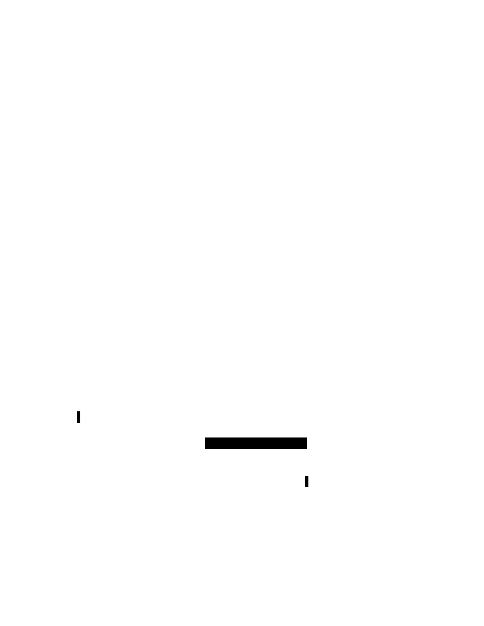
line that is almost everywhere black; Gretel accepts a bet that pays

$1 on black and -$2 on white. Together, Hansel and Gretel incur a

sure loss of $1.

This thought experiment has two significant methodological flaws that are

conceptually unrelated to infinite decisions. First, the use of two independent

agents (Hansel and Gretel) is problematic, because it is unsurprising that two

independent agents who share an initial epistemic state can be led to different

epistemic states by exposing them to different pieces of evidence. Given this, it is

no more surprising that a bookmaker can make a sure profit from the two

agents by arbitraging the difference in their betting prices. This does not seem

like it should count as a Dutch Book, that is to say, as evidence against a decision

rule.

More significantly, the rule Hansel and Gretel seem to be applying — “if one’s

prior credences are P, and one is told that E is the case, then one should update

to credences P ′ such that P ′(H) = P(H | E)” — is invalid. The error has to do with

individuation of propositions: the evidence is not simply E, but the fact that one

was told E. A famous case where this distinction is relevant is the Monty Hall

problem:

Monty has three boxes, red, blue, and green; he chooses one

uniformly at random and puts a valuable prize in it, then seals them.

He then offers you the box of your choice. Once you have selected it,

but before you are allowed to open it, at least one of the remaining

boxes is empty. Monty chooses a box uniformly at random from the

set of remaining empty boxes and opens it. Then he offers you the

opportunity to exchange your box for the third, as yet untouched,

box. Should you accept?

Initially, the objective distribution of the location of the prize is P(R) = P(G) =

P(B) =

. Suppose that one initially selected the red box, and that Monty then reveals

that the green box is empty. It is an error of reasoning to update simply by

conditioning on ¬G and setting . When one conditions

on the full piece of evidence, i.e.,

“I chose the red box, then Monty chose the green box and opened it, revealing

that it was empty”, it can be seen that P ′(R) is still and one is rationally

required to switch boxes. Similarly, Hansel and Gretel should not be conditioning

on the simple content of Lucy’s announcement (“the dart landed within a

vertical line that is almost everywhere black”), but on the fact that Lucy is

announcing the proposition — and since she would announce this in any case,

the announcement has no evidentiary value at all.

Arntzenius et al. give a variant of the dartboard case, motivated by the desire

to eliminate the use of nonmeasurable sets; it also avoids the two problems just

described. However, it has another significant weakness: unlike the other five

scenarios, it relies essentially on the use of an uncountable package of bets. Since

on the standard Kolmogorov account of probability, probability measures are

not uncountably additive, it is unsurprising that one can construct Dutch Books

out of such packages. For example, if we return to the unit square dartboard and

consider the family of bets B(x,y) that pay $1 if the dart lands on (x,y), an agent

whose credence is uniform over the dartboard will value each such bet at $0, but

the package of all such bets at $1. This gives rise to a trivial Dutch Book, one that

does not differ from the more elaborate case given by the authors in any

important respect.

Returning to the first magic dartboard: it can be seen that no open ball (i.e.,

the interior of any circle, no matter how small) on the dartboard is entirely

white or black; every such ball contains uncountably many black and white

points. This gives us a hint of a third potential objection to the case. Not only

does it require that the tip of the dart be infinitely small, we must measure its

location on the board with infinite precision: there is no nonzero margin of error

for the measurement such that we can be certain that the dart landed on either

white or black. The idea that settling such a bet requires the collection and

processing of an infinite amount of data (the infinite number of decimal places to

which one must measure the dart’s coordinates) will be the focus of my critique

of the three remaining cases and the ur-case “Satan’s apple”.

Gambles requiring infinite information

Let’s return to “Satan’s apple”. It is easy to imagine an Eve who submits her

decisions in the form of an algorithm or rule, from which Satan can

independently compute or derive the set of pieces she wishes to take. But doing

so is a form of binding: announcing the algorithm or rule binds Eve to the

resulting set of actions. Let us initially grant the claim that an Eve who cannot

bind is possible — that it is possible, according to some relevant notion of

possibility, for Eve to actually make an infinite number of consecutive decisions,

one for each piece of the apple.

Two essential properties of the case must be emphasized. One is that the

premises require an infinite sequence of consecutive, i.e., non-concurrent,

questions and answers. Otherwise, Eve’s causal dominance argument is invalid:

to apply it, she must be able to reason about a well-defined set of past actions

and whether an additional, logically independent, action will cause expulsion.

The second is that Satan must actually receive and process an infinite number of

those decisions. In the problem as originally formulated, he must receive each

individual decision, since each such decision determines whether Eve should be

allocated a specific piece of the apple. But even without this element, suppose

that Satan ignores some infinite subset S of the decisions. It is then possible for

Satan to be unable to decide whether Eve merits expulsion, because if she only

takes a finite number of pieces from the complement of S, the outcome logically

depends on the decisions in S.

Now, in their presentation of a related case (“Rouble Trouble”), Arntzenius et

al. suggest conceiving of this process in the following way: Eve makes her first

decision at 11 PM, her second at 11:30 PM, her third at 11:45 PM, and so on. In

this way, at the stroke of midnight she will have completed an infinite number of

decisions. I will argue that the sheen of plausibility this lends to the scenario is

bogus. Each decision Eve makes is a logically independent yes/no decision, i.e., a

separate bit of classical information. And within our own physical reality, it is

impossible for Eve to produce and transmit an infinite number of bits of

information within a finite amount of time. In other words, the notion of

possibility under which non-binding Eve is possible is not physical or

nomological possibility [Shieber, 2014], but some more lenient notion.

Arguing for this requires several different principles of physical theory. First,

there is some distance d > 0 such that if Eve and Satan are to count as

independent agents, they must be separated by at least d. On our current

understanding of quantum mechanics, d is some value on the order (10−35

meters) of the Planck length — not necessarily the Planck length itself, but

something near it. To quote Shieber [2007]: “any attempt to resolve phenomena

below this scale, as would be necessary to store information, would require so

much energy that the region being resolved would collapse into a black hole.”

When we combine this with the impossibility of superluminal signaling

(transferring classical information faster than the speed of light), we derive that

each communication between Eve and Satan must take time at least t for some t

> 0, where t is on the order of the Planck time.

Could Eve get around this by encoding an infinite number of decisions within

a single transmission? The answer is no, by the Bekenstein bound [Bekenstein,

2005]; by similar considerations in the physics of black holes, the amount of

information that can be stored in a system is bounded by a quantity

proportional to the product of the its radius and its total mass-energy. Since the

amount of mass-energy available to Eve and the size of the universe during any

given time interval are both finite, no such transmission is possible. Thus, Eve

requires an infinite number of sequential transmissions to communicate her

decisions. Since there is a lower bound on the time required for each

transmission, she requires an infinite amount of time.

On the one hand, the specific argument I have made is tentative because of

the absence of a definitive theory of quantum gravity. Jordan [2017] cautions

against this sort of analysis because the idea of spatial locality itself may become

problematic at the Planck scale. But regardless of the specifics, our current

understanding of quantum information theory suggests that for several different

reasons, completed infinities like the one in “Satan’s Apple” cannot exist in

nature. This is the case for the infinite precision to which one must measure the

position of the magic dart (because of Heisenberg’s uncertainty principle), and

also for any scenario like “Satan’s apple” that requires an agent to produce an

infinite sequence of decisions. It also suggests that utilities may be bounded, in

principle, by the capacity of the universe to store information.

Does this allow us to deny the relevance of infinite cases as counterexamples

to standard decision theory? Most arguments for or against decision theories,

such as the axiomatic method or Dutch Book arguments, have an a priori

character. Bringing empirical facts into the debate might feel like an intrusion.

But I think this obscures the extent to which decision theories are already tailor-

made to the world we live in. An example is the use of realvalued probabilities

and utilities; I follow Feferman [2009] in regarding the real numbers R as

representing not a “uniquely determined concept”, but a sophisticated

compromise between “geometrical, arithmetical and set-theoretical notions”

designed to support a fruitful pure and applied mathematics. In other words,

they already encode contingent facts about our world, the same way that

Euclidean geometry encodes contingent facts about the behavior of space-time

at the scales directly observable by human beings on Earth.

A different physical reality might demand a quite different mathematical

structure for the representation of value and belief; in particular, agents in a

physical reality that could accommodate infinite decision problems might face

unfamiliar notions of uncertainty and scarcity. Arntzenius et al. [2004] are

aware of the problem and give the following example of an infinitary but non-

probabilistic “free lunch” or “reverse Dutch book”:

Imagine friends f0,f1,f2 ... all standing in a line. For each n, friend fn

gives $n to friend fn−1. After this process is complete, fn has given away

$n and received $(n+1). Each friend earns a profit of $1.

But since decision theories are ways of coping with uncertainty and scarcity,

perhaps it should be unsurprising that different realities might require different

decision theories. I propose the following sequel to “Random Integers”:

“Aha!” cries Satan. “You owe me at least $1!” Gabriel reflects for a

moment. “Wait — if we were able to contract these bets, that implies

that mass-energy isn’t conserved!” Gabriel produces $2 out of thin

air and hands $1 to Satan, saying “keep the change.” “What were you

planning to spend this on, anyway?” asks Gabriel. “I don’t know,”

Satan mumbles with a crestfallen shrug.

2.4 Newcomblike problems

The Newcomb paradigm

Newcomb’s problem [Nozick, 1969] is canonical:

A demon has the ability to perfectly predict your actions. The demon

will enter a room and seal money in two boxes, at which point you

will enter the room and be given the choice between taking the left

box only, or both the left and right boxes. If the demon predicts that

you will take only the left box, she will place $1,000,000 in the left

box and $1,000 in the right. If she predicts that you will take both

boxes, she will place $0 in the left box and $1,000 in the right.

For the purposes of this discussion, a Newcomblike problem is one that

violates the premises of Savage’s representation theorem by having states

depend on acts. (In the paradigmatic example, whether the $1,000,000 is in the

first box is a state of the world, but whether it is the case depends on the agent’s

act of taking one box or two.)

The problem is commonly described as distinguishing between causal and

evidential decision theory (hereafter CDT and EDT). Since taking one box is

associated with receiving $1,000,000 and taking both is associated with

receiving $1,000, the evidential decision theorist takes one box and gets rich.

But no matter what the contents of the boxes are, taking the right box yields an

additional $1,000 — therefore two-boxing is the dominant option at the time of

the decision, and the causal decision theorist chooses it, receiving only the

smaller sum. Meanwhile, the causal decision theorist who can bind to an action

will bind at the outset to one-boxing — the predictor will then recognize this

and the agent will receive $1,000,000 after all.

Now, this problem seems to be entangled in some thorny questions related to

free will. As Aaronson [2013a] and others have observed, the setup of the

scenario seems to equivocate as to whether the agent has free will —

specifically, a certain kind of libertarian free will, the pre-analytic concept of

which is something like “the ability to do otherwise”. Here is an approximate

reconstruction of this argument:

We suppose that the predictor is always accurate. When I’m in the

room, the predictor has already fixed her prediction, either that I will

one-box or that I will two-box. Suppose first that she predicted that I

will one-box. Now, if I were to two-box, her prediction would be

wrong, which is a contradiction. Therefore, it must be that I will one-

box — so at this time, I in fact lack the ability to two-box. Likewise, in

the case where she has predicted where I will two-box, I don’t have

the ability to one-box. So in either case, I’m not actually making a

decision; my choice is already constrained. This contradicts the

framing of the scenario as a decision problem.

But this same objection seems to apply “one level up”, so to speak — it can be

used to attack the relevance of the problem to the debate as to whether one

should adopt CDT or EDT. The “why ain’tcha rich” argument for EDT goes

something like this:

If you use CDT in Newcomb’s problem, you get $1,000. If you use EDT, you

get $1,000,000. So you should adopt EDT.

But the skeptical adherent of CDT may reply:

If I accept the premises of Newcomb’s problem, then when I’m in the

room I lack the ability to choose between one-boxing and two-

boxing. So why should I suppose that I currently have the ability to

adopt EDT? By arguing as you have, you seem to be displaying an

implicit commitment to the idea that I do have this ability. But then

you owe me an explanation of why I have free will to adopt EDT, but

not to violate the premises of the Newcomb scenario.

I am sympathetic to CDT and accordingly I would like very much to dismiss

Newcomb’s problem as an argument against it. And as before, I am unimpressed

by the mere metaphysical possibility of the Newcomb case. In order to count

against CDT, the Newcomb case should in fact be nomologically possible in some

form. But if it is nomologically possible, then I am sympathetic to “why ain’tcha

rich” as an objection to CDT — if $1,000,000 is up for grabs, something is very

wrong with a decision theory that leaves $999,000 on the table.

Can “why ain’tcha rich” be saved from the skeptic’s reply?

In what follows, I will examine two settings in which it appears that

Newcomb’s case is in fact nomologically possible and furthermore “why ain’tcha

rich” is a sound argument against CDT, one that succeeds against the skeptic’s

reply. Therefore, EDT is recommended over CDT in these settings. But CDT with

binding is recommended over CDT in them for the same reasons — and,

contrary to an argument of Meacham [2010], I will argue that CDT with binding

is recommended over all competing decision theories in Newcomblike

problems.

Two common features of both settings are necessary to support this analysis.

One, as in the analysis of Burgess [2004], is common causation — the initial state

of the agent (and the world) causes both the demon’s infallible prediction and

the agent’s decision. The second is that the agent’s initial state — unlike the

agent’s actual “in-room” decision, which is causally determined — is plausibly

subject to some form of libertarian control. I won’t argue that every conceivable

setting for the Newcomb problem has these features, nor that every

nomologically possible setting must have them. But since the two

aforementioned settings effectively exhaust all the possibilities I’m aware of, I

hope to put the ball in the other court — it will be for the defender of an

alternate account of Newcomb cases to advance a nomologically possible setting

that provides a counterexample.

Binding as decision theory adoption

I claim that there is something special about CDT with binding — namely, it

formalizes the metatheory in which we debate which decision theories to adopt,

and in which arguments like “why ain’tcha rich” function. To see this, compare

the “Smoking Lesion” argument against EDT:

Abigail would like to start smoking, because it is pleasurable (it has

utility 10). In Abigail’s world, smoking is highly correlated with

cancer (utility −1000), but it does not cause cancer. Rather, there is a

certain brain lesion that causes both a desire to smoke and cancer —

so for an arbitrary member of the population, P(cancer | smokes) =

.9 and P(cancer | ¬smokes) = .1. Thus, according to EDT, the utility of

not smoking is P(cancer | ¬smokes) · u(cancer) = −100 and the utility

of smoking is P(cancer | smokes) · u(cancer) + u(smokes) = −890.

Abigail therefore decides not to smoke.

The problem with Abigail’s reasoning is that her decision to not to smoke is

not causally effective in reducing her risk of cancer — as Lewis [1981a] puts it,

she is simply “managing the news”. In fact, Abigail should be analyzing her

situation with CDT, which tells her to smoke via the same kind of dominance

reasoning that leads to two-boxing in the Newcomb case; since smoking has no

causal influence on cancer, smoking gives her 10 additional utiles whether or

not she has cancer, so she should smoke.

Now, if Abigail adheres to CDT, one plausible (but not necessary) reading of

her situation is that her desire to smoke is evidence that she has the lesion and

cancer, i.e., P(cancer) = .9. Therefore, according to CDT, the utility of not smoking

is P(cancer)·u(cancer) = −900, and the utility of smoking is P(cancer)·u(cancer)

+u(smoking) = −890. Thus, the expected utility under CDT of the action

recommended by CDT (smoking) is much lower (−890) than the expected utility

under EDT (−100) of the action recommended by EDT (not smoking).

This is superficially parallel to Newcomb’s problem, where the CDT-utility of

the CDTrecommended action ($1000) is lower than the EDT-utility of the EDT-

recommended action ($1,000,000). But the parallel breaks down because in

Newcomb’s problem (at least, in settings for Newcomb’s problem that conform

to the aforementioned common-cause analysis), adopting EDT causally leads to

the million dollars — by way of causing the agent to predict that you will one-

box. But for Abigail, adopting EDT and deciding not to smoke has no causal effect

in getting her to the preferred outcome. From our privileged vantage point in the

metatheory, we can see that Abigail’s EDT-utility is fool’s gold.

Can we formalize this metatheory? I claim that the metatheory in which we

benchmark decision theories against “why ain’tcha rich” arguments is exactly

CDT — a decision theory is recommended exactly in the cases where adopting it

causally leads to the preferred outcome. As evidence, I can adduce that this

correctly describes every argument by counterexample against a decision theory

in the literature that I’m aware of:

1. As discussed above, the original Newcomb scenario, interpreted as an

argument against

CDT

2. “Smoking Lesion” against EDT

3. The “World Series” scenario in Arntzenius [2007] against EDT

4. The “Evidential Blackmail”, “Counterfactual Blackmail”, and “Retro

Blackmail” scenarios in Soares and Fallenstein [2014]

But now, we can see that CDT with binding performs at least as well as every

other decision theory. Suppose adopting decision theory D causes you to reach

outcome X. Then, CDT with binding can see that binding to the D-recommended

action — at the same point of the causal history at which D itself could have

been adopted — is also causally effective in reaching outcome X. By this

“strategy-stealing” argument, CDT with binding must be “complete” against this

class of problems. No matter what your preferences are, if they can be achieved

by any decision theory, they can be achieved by CDT with binding.

What might a “why ain’tcha rich” counterexample against CDT with binding

look like? Decision scenarios seem to have a type hierarchy, in the following

sense: in the original Savage paradigm (call this the “zeroth order”), the

uncertain state of the world is independent of your acts. In the Newcomb

paradigm (the “first order”), the state may depend on your act. By the strategy-

stealing argument, CDT with binding should succeed against all

counterexamples at this level. To defeat it, we seemingly have to go to “second-

order” counterexamples that examine not merely the agent’s acts, but their

reasons for choosing acts:

A demon has the ability to perfectly predict your actions — and

moreover, to inspect your reasons for performing those actions. The

demon will enter a room and seal money in two boxes, at which

point you will enter the room and be given the choice between taking

the left box only, or both the left and right boxes. If the demon

predicts that you will take only the left box, because you chose to do

so via EDT or for pre-theoretic reasons, she will place $1,000,000 in

the left box and $1,000 in the right. If she predicts that you will take

both boxes, or you will take one box because you chose to do so via

CDT with binding, she will place $0 in the left box and $1,000 in the

right.

This demon certainly seems metaphysically possible. But this seems like an

unconvincing counterexample, for two reasons. One is that it is unfair — the

agent is being punished not for anything he does, but purely for having adopted

CDT with binding. Compare the response of Lewis [1981b] and others to the

original Newcomb case, that the “why ain’tcha rich” argument against CDT is

invalid because the demon simply punishes rationality (of which CDT is the

correct analysis) and rewards irrationality; therefore the rational agent cannot

hope to to succeed. Again, I think that with regard to the original first-order

Newcomb problem, this is unconvincing. But as an objection to second-order

problems of this type, it is more convincing because no matter what your

decision theory is, there exists a demon that has singled you out for this kind of

punishment, based simply on who you are.

The other is that adversaries plausibly have more reasons to care about the

agent’s actions than they do to care about the agent’s reasons. A good example is

the “Counterfactual Blackmail” scenario in Soares and Fallenstein [2014], which

is isomorphic to Newcomb’s problem, but in which the “demon” has realistic

motivations. I paraphrase:

You and an adversary who can predict your actions are playing the

stock market. The adversary develops a virus which will affect

market operations and cause a massive market crash, which will cost

both of you $150,000,000. Once the virus has been deployed, there is

a 24-hour window in which it can be stopped; because of the way it

is programmed, the only way to stop it for you to pay the adversary

$100,000,000. But the adversary is risk-averse and will only deploy

the virus if she predicts that you will respond by paying.

To make explicit the connection to Newcomb’s problem, paying is like two-

boxing: once the virus has been deployed, paying causally saves you

$50,000,000. But a precommitment to not paying, or the adoption of a decision

theory which dictates not paying, causally prevents you from being blackmailed

at all.

I think the force of “Counterfactual Blackmail” is that it shows a Newcomb

demon with reasonable motivations — all it cares about is money, and its acts

are aimed at maximizing its money. Consequently, the demon cares about the

agent’s acts, because one of those possible acts is giving the demon money. In

contrast, the demon from our second-order counterexample seems to be

motivated by a sort of holy war against CDT with binding. And, independently of

any questions of fairness, this is less plausibly the kind of adversary that an

agent will come to face.

The AI setting

LaVictoire et al. [2013], working in the context of artificial intelligence, develop a

theoretical model in which a group of artificially intelligent agents have access to

each other’s source code. It is then possible for the agents to prove properties

about each other, for example, that an agent faced with Newcomb’s problem will

one-box or that an agent faced with the Prisoner’s Dilemma will cooperate and

not defect. This gives rise to a novel strategy for the Prisoner’s Dilemma:

cooperate if and only if you can prove that your opponent will cooperate. This

strategy achieves cooperation against a variety of well-intentioned agents,

including itself, but defects against agents that are malicious or simply

impenetrable to its proof techniques. Translating this model into the context of

Newcomb’s problem, we can imagine a demon that reads an artificial agent’s

source code, then puts the $1,000,000 in the left box if and only if it can prove

that the agent will one-box.

This is, then, a nomologically possible setting for Newcomblike problems.

Moreover, it satisfies the two requisite conditions in a straightforward way. The

agent’s action and the demon’s prediction both have a common cause, namely,

the initial source code and state programmed into the agent by its programmers.

Moreover, there is no contradiction between the programmer having libertarian

control over the source code and the demon’s ability to make perfect

predictions, from the code, about the resulting agent.

The problem of formulating an ideal decision theory for a related model is

explored in detail by Soares and Fallenstein [2014], who consider and reject an

analogue of CDT with binding, then focus on a novel decision theory called

“updateless decision theory”, or UDT. One of their claimed counterexamples to

CDT with binding is called “Retro Blackmail”, and the idea at its core is that

binding is no longer causally effective if the adversary’s prediction starts in the

agent’s causal past. For simplicity, I will translate the scenario into the language

of the original Newcomb problem:

An agent was originally programmed to obey CDT with binding, and

it is evolving in a deterministic environment. It is currently faced

with the Newcomb scenario. However, the demon will make its

prediction by simulating the agent using its original source code and

state — because of determinism, this prediction will still be perfectly

accurate. The agent reasons that binding to one-boxing (which is

how it would respond to the original Newcomb scenario) is now

causally ineffective, because making a precommitment now has no

causal effect on a simulation beginning from an earlier snapshot of

itself. The agent therefore makes no precommitment, enters the

room, two-boxes according to causal reasoning, and receives $1,000.

Meanwhile, UDT tells the agent to one-box, consequently achieving the

$1,000,000. Is this a counterexample to the strategy-stealing argument for CDT

with binding? I don’t think so, but the scenario is very informative about the

argument and about the challenges of implementing CDT with binding.

Programming the agent to obey UDT (or EDT) causally leads to one-boxing,

which causally leads to the $1,000,000. Therefore, CDT with binding can steal

the strategy and pre-commit to one-boxing, but only at the same point in the

causal history at which adopting UDT would have been causally effective,

namely the time of the agent’s original programming. In order to function

correctly, CDT with binding must be able to form binding precommitments at

the absolute beginning of the agent’s causal history (in this case, the time of

original programming) — or, at any rate, the earliest point in the causal history

visible to the predictor. If this is not done correctly, then the agent will be

vulnerable to “retro” scenarios where the prediction occurs prior (in the causal

sense) to the act of binding. But if it is, the act of binding will cause both the

agent and every veridical simulation of the agent to one-box, and the agent will

receive $1,000,000 after all.

If we neglect the problem of logical omniscience, then there is no difficulty in

imagining the agent precomputing every causally recommended

precommitment simultaneously with the moment of its original programming.

But since there are infinitely many such precommitments, corresponding to the

infinite space of potential Newcomblike cases, the problem is too pressing to set

aside so blithely. Fortunately, it seems that we can produce an agent equivalent

in behavior to this ideal agent, but which does not have to store an infinite

number of precommitments; instead, it will compute the same precommitments

“on the fly” via lazy evaluation. Whenever the agent is faced with a decision

problem, it can reason that CDT with binding has already precommitted it to one

of the available actions, and it can compute which action it is via causal

reasoning that starts at the beginning of its own history — it can iterate over all

the precommitments and pick the one causally recommended at that time. There

are still many barriers to precisely specifying and implementing CDT with

binding, but hopefully this represents some measure of progress.

Is there an ideal decision theory?

One might, however, question whether a complete and coherent set of causally

recommended precommitments (alternately, a coherent decision theory that is

optimal with respect to all Newcomblike problems) is possible. Call the

following scenario “Newcomb’s Angel”:

An angel has the ability to perfectly predict your actions. If she

encounters you, she predicts what you would do when faced with

Newcomb’s demon, then gives you the opposite payoff: $1,000,000 if

you two-box and $1,000 if you one-box. (The kind of prediction being

invoked here — unlike the kind in the original Newcomb problem —

is incompatible with a definition of prediction as “knowledge of

future events”. But it is compatible with any Burgess-type common

cause setting, including the settings discussed in sections 2.4 and

2.4.)

On the one hand, Newcomb’s Angel is intuitively less persuasive as a scenario

than Newcomb’s Demon. For one, the agent doesn’t seem to have the same kind

of veridical information about the situation as in the original case. Another issue

is that we can construct such an angel rewarding any behavior, including

behaviors that seem uncontroversially irrational (intransitive preferences,

perhaps). Finally, as discussed previously, the demon case has an isomorphic

variant, “Counterfactual Blackmail”, where the demon-analogue has realistic

motivations. And it’s difficult to imagine such a setting for the angel.

Nonetheless, there does seem to be a dilemma here. A decision theory

succeeds on Newcomb’s Angel if and only if it fails on Newcomb’s Demon. And

the strategy-stealing argument lets CDT with binding match the performance of

any such theory, but it doesn’t choose which scenario one should succeed on. At

the least, if “why ain’tcha rich” does serve to justify a precommitment to one-

boxing in the original Newcomb problem, it must be an implicit premise of that

scenario that the world isn’t populated by Newcomb angels, or that it has fewer

Newcomb angels than Newcomb demons.

Significantly, I think Newcomb’s Angel succeeds in undermining a certain

argument for one-boxing in the original problem. I paraphrase Aaronson

[2013b]:

Suppose Newcomb’s demon can accurately predict whether you will

one-box or two-box, no matter how you reach your decision. Since

your decision-making process can rely on arbitrary memories and

involve arbitrary thought processes (e.g., you might decide to one-

box if and only if the number of students in your kindergarten class

was odd), the demon must have, de facto, the ability to simulate your

entire consciousness — the demon possesses the functional

equivalent of a simulated copy of you. It follows that when about to

enter the demon’s room, you should be indifferent as to whether you

are your original self or the simulated copy. Therefore, you should

one-box, because if you are in fact the copy, your one-boxing will

causally lead to your counterpart receiving the $1,000,000.

For now, I will leave aside the questions about personal identity raised by

this argument — they will come into focus in section 2.4. Even if one accepts the

identification between the real-world agent and the agent as simulated by the

demon, Newcomb’s Angel illustrates that the simulated agent is unjustified in

believing that his one-boxing benefits his real-world counterpart: if an angel and

not a demon is on the other side of the veil, then he is harming his counterpart,

not helping.

A natural response is to say that the simulated agent should one-box if he

believes that his counterpart is facing the demon, and two-box otherwise. But I

think this response fails. Given that he is, after all, in a simulation, none of the

agent’s evidence about the true state of the world is trustworthy. The angel can

go to arbitrarily lengths to persuade him that he is in fact facing the demon —

take him on an ersatz journey to a part of the universe with demons and no

angels, or show him a celestial war in which the demons exterminate the angels.

Moreover, the non-veridicality of these experiences has a counterpart in the

Newcomb’s Demon case: there too, the simulated agent is being deceived about

an essential aspect of the case, because money has not already been sealed in the

boxes, those inside the simulation or out of it. Once the possibility of being in a

simulation is on the table, I think the correct attitude to questions about events

outside the simulation is a kind of radical skepticism.

The brainscan setting

Meanwhile, a long-running discussion in the literature, starting with Lewis

[1979] and continuing notably with Burgess [2004] and Aaronson [2013a],

considers a setting for the Newcomb problem based on the idea of physical

simulation of the agent. Specifically, it is consistent with known laws of physics

that Newcomb’s demon can measure a sufficiently precise physical description

of the agent’s body, then use this description to simulate the agent’s actions

according to quantum mechanics. If this is in fact physically possible, then we

can assume that the demon has “black-box” or “sampling” access to arbitrarily

many independent copies of the agent. She can then predict that the agent will

one-box (likewise two-box) exactly in the cases where a sufficiently large

number of independent simulations all result in the agent picking one box.

Now, several things could go wrong with this picture. Aaronson [2013a] is

interested in the empirical possibility that such prediction will turn out to be

physically impossible, because human actions may physically depend on the

measurement outcomes of uncollapsed quantum states, which the predictor

cannot simulate because copying them would violate the no-cloning theorem. If

this is so, then it is impossible to make even probabilistic predictions about an

agent’s actions via this technique. But the possibility I will be concerned with

here is that such predictions are possible, but due to physical indeterminacy

they are, at least in the worst case, probabilistic. That is to say, a series of

physically accurate simulations of an arbitrary agent may result in the agent

one-boxing in some of the trials and two-boxing in the others.

How should the demon respond to such a simulation result? Nozick’s original

exposition considers the question of an agent who decides whether to one-box

or two-box by flipping a coin (the result of which is assumed unpredictable in

advance by the demon). Nozick suggests that the demon should simply detect

this and punish this agent by refusing to put money in either box — this

preserves the scenario because the strategy “flip a coin” is now strictly

dominated by other strategies and can be disregarded. Meanwhile, Aaronson has

suggested that the demon should respond by placing the $1,000,000 in the left

box with the same probability p with which the agent one-boxes in the trials.

Thus, indeterminate decision processes form a continuum between “always one-

box” and “always two-box”, but the first of these is still the worst and the second

is still the best.

This gives rise to a concrete physical characterization of what “binding”

means, albeit one that conflates it with other states. “Binding to one-boxing”

implies being in a physical state, at the time of the brainscan, that causally

determines (with very high probability) that you will one-box. Now, this

characterization also plausibly describes some mental attitudes that we would

consider distinct, for example, “having propositional attitudes that constitute

reasons to one-box”, or “evaluating the Newcomb scenario via EDT.” But,

following Balaguer [2010], I think it’s an empirical question for neuroscience

(one which can be attacked via ambitious but scientifically grounded programs

such as whole-brain emulation) what these brain-states are, and under what

circumstances people faced with a Newcomb scenario come to be in them. Then

it’s a subsequent empirical question for psychology what mental attitudes and

phenomenal experiences these brain-states correspond to.

Given this, I want to describe one possible way these investigations could

turn out, a way that would validate the intuitions of frustration that CDT-

inclined people like me have with the Newcomb problem. Of course, there is no

guarantee that this will be the empirical result, nor are these intuitions evidence

for what the result will be. But it’s empirically possible that if someone is fully

informed about the scenario and models it according to Burgess’s common-

cause characterization, then the only initial brainstates which determinately

lead to one-boxing are ones where she “decides not to think”, e.g., she resolves to

march into the room with her eyes shut and grab the left box. On the other hand,

if she enters the room willing to contemplate the problem, the outcome of this

deliberative process may be physically indeterminate — she may end up one-

boxing in some trials and two-boxing in others. Under Nozick’s formulation, this

will result in her receiving no money, even if she does end up one-boxing. Under

Aaronson’s, this behavior is straightforwardly seen to be undesirable because

the agent can maximize expected utility by maximizing the probability that her

initial brainstate leads to one-boxing — therefore, “deciding not to think” is

causally recommended. But regardless of whether this specific possibility seems

likely, I hope that it calls into question intuitions about the relationship of

Newcomb’s problem to experiential facts about reasoning, since we can hope for

empirical research that will clarify the question.

Now we come to the claimed counterexample of Meacham [2010] against

CDT with binding:

But self-binding causal decision theorists can still end up poor.

Consider a version of the Newcomb’s case where the predictor

makes her prediction before the agent is born. The binding causal

decision theorist will be unable to causally influence the prediction,

and so she will end up choosing both boxes and getting only a

thousand dollars. So even when we restrict our attention to agents

who can bind themselves, the “why ain’cha rich” argument against

causal decision theory remains.

This scenario is recognizable as “Retro Blackmail”, translated into the

brainscan setting. But in this context, we are fully equipped to reject its

premises. In particular, the scenario implies that it is physically determined

before the moment of birth whether a human will eventually adhere to EDT or

CDT (or to some other decision theory, or to neither). But this is

straightforwardly implausible. Consider, for example, a lottery for course

assignments, on which it stochastically depends whether Zeke studies decision

theory during the fall semester from a professor who advocates CDT, or in the

spring semester from a professor who advocates EDT. Thus, in the Nozick

formulation, the demon will simply never award any money.

In the Aaronson formulation, however, the questions about personal identity

that have been lurking in the background take center stage. The demon will

predict you via her probabilistic sampling access not only to the possibilities for

your own actions, but also the possible actions of other people — the people

whom your embryo might have grown into under other circumstances. What,

then, should you do? The two extreme cases are instructive: if there’s only one

way you could have turned out, then everyone the demon can sample is a copy of

you, and we’re back in the original Newcomb case and you should one-box. But if

you are, as it were, one of a great multitude of possible selves — and the

reasoning of those other selves is not identifiable with yours — then it’s as

though the demon were predicting your actions via a population statistic, and

because of the lack of a causal connection between your attitudes and the

outcome of the prediction, you should two-box. (Compare, for example, a demon

who knows that 95% of Oregonians are one-boxers, and therefore seals money

in the left box with probability .95. This is a probabilistically accurate predictor,

but nonetheless, as an Oregonian facing her, you should two-box.),

Between these two points lies a continuum. If you control, so to speak, more

than of the vote — if your decision is identifiable in a physical

sense with the

decision of more than of your possible selves — then your one-boxing

contributes more than $1,000 in expected value to your payoff and you should

do it. But if you control less than that, then your contribution would be too small

to outweigh the certainty of $1,000, and you should two-box. I think this is a

graphic illustration of a general problem: the more we generalize Newcomb’s

Problem and generalize our decision theories to compensate, the more we

should expect difficult detours into metaphysics, in questions of both free will

and personal identity.

2.5 Conclusion

At many points in this discussion, I have disputed the value of binding as a

solution to one decision-theoretic paradox or another. But even if binding could

solve all of these paradoxes, I think that it still would not constitute a single,

unified correction to decision theory — the paradoxes have conceptually distinct

grounds, and therefore inasmuch as binding can solve them, they are solved by

conceptually distinct notions of binding. Just as a genuine philosophical

unification can illuminate philosophical data, a spurious unification can obscure

them.

2.6 Acknowledgements

I am indebted to Lara Buchak, Peter Epstein, Paul Christiano, Scott Aaronson,

Nate Soares, Melissa Fusco, and Mikayla Kelley for helpful discussions.

Chapter 3

Frequentism as a positivism: a

three-tiered account of probability

Abstract

I explore an alternate clarification of the idea of frequency probability, called

frequency judgment. I then distinguish three distinct senses of probability —

physical chance, frequency judgment, and subjective credence — and propose

that they have a hierarchical relationship. Finally, I claim that this three-tiered

view can dissolve various paradoxes associated with the interpretation of

probability.

3.1 Introduction

Frequentism and its challenges

Frequentism means, more or less, that probabilities are ratios of successes to

trials. It originates with John Venn and is arguably the first philosophically

rigorous account of probability — that is to say, it is the first account of

probability to appear as an attempt to correct a philosophically inadequate pre-

theoretic view. As Alan H´ajek has observed, however, it has fallen on hard times.

In part, this is because it competes with the Bayesian interpretation of

probability, in which probabilities are subjective degrees of belief. Bayesianism

offers a seductive unifying picture, in which epistemology and decision theory

can both be grounded in a quantitatively precise account of an agent’s attitudes

and propensities. But frequentism’s philosophical difficulties are not simply due

to its being outshone by a competing view. As Ha´jek has shown, frequentism

itself faces a variety of vexing challenges.

Ha´jek reconstructs frequentism as containing two distinct conceptions of

probability — finite frequentism, in which probabilities are actual real-world

ratios of successes to trials, and hypothetical frequentism, in which they are

limiting relative frequencies over an idealized hypothetical infinite sequence of

trials. In a series of two papers [1996, 2009], he shows that each conception is

affected by numerous difficulties: in fact, each paper gives 15 distinct objections

to one of the conceptions!

In order to motivate what follows, I’ll briefly summarize what I consider the

most pressing of H´ajek’s objections against each characterization. Finite

frequentism is intuitively appealing because of its metaphysical parsimony;

probabilities can be “read off” from the actual history of real-world events,

without the need to posit any unobservable entities. But taken literally, it clashes

with many of our important intuitions about probability. In particular, it is a kind

of operationalism about probability, and hence suffers from similar problems to

other operationalisms. If we consider probability to be defined by real-world

frequency, then we have seemingly have no way to express the idea that an

observed frequency might be aberrant, just as defining temperature to be

thermometer readings leaves us with no way to express the idea that our

thermometers may be inaccurate. This problem becomes especially serious

when we consider cases where the number of real-world trials is very small —

in particular, if there is only 1 trial, then the finite frequency probability must be

either 0 or 1, and if there have been no trials yet, then it is undefined. Finite

frequentism is in conflict with our intuitions that actual trials constitute

evidence about probability rather than its actual substance.

Hypothetical frequentism answers this concern perfectly, but at far too high a

metaphysical cost. In particular, asserting the existence of an infinite sequence of

trials seems to involve an “abandonment of empiricism.” In the real world, we

cannot perform an infinite sequence of trials, so the meaning ascribed to

probabilities is evidently counterfactual. Even after granting this, what kind of

counterfactual are we dealing with? If we analyze it using a possible-world

semantics, in the style of Stalnaker or Lewis, we seemingly require a possible

world that (at the very least) violates the conservation of mass-energy. Why

should we believe that probabilities in this world have anything to do with ours?

Finally, the following objection is commonly advanced against both

conceptions of frequentism: frequentism entangles the probability of any

individual event E with the question of what will happen to other, similar events.

We cannot make frequentist sense of the probability of E without assigning it to

some broader reference class of events, over which we will be able to define a

ratio of successes to trials. But at this point, P(E) will be a property of the

reference class, not of E itself. This objection is already troubling, but it has even

more teeth in cases when there are multiple possible reference classes, each

yielding a distinct value of P(E), or perhaps no reference class at all. This is the

so-called “reference class problem”, and it is another, crucial sense in which

frequency notions of probability diverge from our ordinary understanding of the

word.

Where to?

I am a frequentist. What sort of frequentist am I? Of the two varieties

distinguished above, I am much more sympathetic to finite frequentism; the

metaphysical costs of infinite hypothetical sequences are too much for me to

bear. In fact, I think that finite frequentism, properly expounded, can actually

escape many of the criticisms Ha´jek levels at it — perhaps eight out of fifteen.

But I cannot deny the force of Ha´jek’s overall arguments, and I think it

inevitable that I must give some ground. Specifically, I think an adequate analysis

of probability must both seek a third way of defining frequency probability and

also acknowledge that not all probabilities are frequency probabilities. Here are

some of my desiderata for such an expanded conception:

1. It should preserve core frequentist intuitions that relative frequency is an

essentialcomponent of probability. In particular, it should not conflate

probabilities that have an intuitively acceptable frequency interpretation

(e.g., the probability that a U.S. quarter, when flipped, will land heads) with

those that do not (e.g., the probability referenced in Pascal’s wager that

God exists).

Indeed, the primary goal of this paper is to propose and defend a definition

of frequency probability that is both reasonably rigorous and free from

paradox, in hopes that it will enable epistemological views in which

frequency probability has a privileged status.

2. It should not take a stance on the existence of physical chance (something

which posesproblems for both frequentist and Bayesian accounts of

probability). I think that a proper resolution of this question rests on

questions external to the philosophy of probability, in particular on the

philosophy of physics, and that consequently it is an advantage for an

account of probability to remain agnostic on the question.

3. It should not deny the validity of the Bayesian interpretation of probability

outright.As Jaynes [1985] remarked, arguing in the reverse direction:

I do not “disallow the possibility” of the frequency

interpretation. Indeed, since that interpretation exists, it would

be rather hard for anyone to deny the possibility of it. I do,

however, deny the necessity of it.

Indeed, while I consider myself a frequentist, I affirm the value of Bayesian

probability, both its technical validity as a consistent interpretation of the

laws of probability and as the correct solution to certain epistemological

problems such as the preface paradox. My skepticism is confined to claims

such as the following: all probabilities are Bayesian probabilities, all

knowledge is Bayesian credence, and all learning is Bayesian

conditionalization. I will say more about this later.

4. At the level of statistical practice, it should support a methodological

reconciliationbetween frequentist and Bayesian techniques. That is to say,

it should acknowledge that in practice both methods are effective on

different problems, independently of the philosophical debate. Kass [2011]

calls this viewpoint “statistical eclecticism” and Senn [2011] calls it

“statistical pragmatism”.

5. Thus, it is necessary for it to preserve the distinction between frequentist

and Bayesianmethods, that is to say, between methods that make use only

of probabilities that have

a natural frequency interpretation and those which make use of prior

probabilities that do not. Otherwise, frequentist and Bayesian methods are

collapsed into a single group, in which frequentist methods appear merely

as oddly restricted Bayesian methods.

Without further ado, I will introduce an account of probability that I believe

will fulfill all these criteria. The argument will necessarily detour through many

philosophical considerations related to probability. The reader who is pressed

for time should look at sections

3.2, 3.4, and 3.5.

Precedents for the view

The closest historical precedent I am aware of for my view is Carnap’s

distinction [1945] between two senses of probability: Probability1, which

describes credence or degree of confirmation, and Probability2, which describes

long-run relative frequency over a sequence of trials. In particular, he makes the

following parenthetical remark about Probability2 (M1 denoting a class of trials

and M2 an event):

I think that, in a sense, the statement ‘ ’ itself may be

interpreted as stating such an estimate; it says the same as: “The best

estimate on the evidence e of the probability2 of M2 with respect to M1

is 2/3.” If somebody should like to call this a frequency

interpretation of probability, I should have no objection.

My view differs substantially from Carnap’s in almost all respects — in

particular, I will not make use of the notion of logical probability that he

advocated. Nevertheless, I will interpret this remark as Carnap’s blessing.

3.2 The theory

Three conceptually distinct interpretations of probability suffice to describe all

uses of probability. They are arranged in a tiered hierarchy as follows:

1. Physical chance, if it exists. This is the only objective and metaphysically

real kind ofprobability.

2. Frequency judgments. Pending a more precise motivation and definition,

the core ideais this: given an event E, a frequency judgment for E is a

subjective estimate of the proportion of times E will occur over an

arbitrarily large (but finite) sequence of repeated trials. This is intended as

a frequency interpretation of probability, i.e., one that can replace finite

and hypothetical frequentism.

3. Bayesian subjective probability in the sense of Ramsey and de Finetti.

Probabilities pass “downwards” along this hierarchy in the following sense:

1. If an agent knows a physical chance (and no other relevant information),

that agent isobliged to have a frequency judgment coinciding with the

physical chance.

2. If an agent has a frequency judgment (and no other relevant information),

that agentis obliged to have a Bayesian subjective probability coinciding

with the frequency judgment.

Thus, as we pass down the hierarchy, the domain of applicability of the

interpretations strictly increases. In particular, the conjunction of the two

relations yields a large fragment of (possibly all of) Lewis’s Principal Principle.

3.3 The first tier: physical chance

Lewis [1994] defines chance as “objective single-case probability”, which does

an excellent job of explaining why chance is so vexing for both frequentists and

Bayesians. For one, a chance is a probability that we intuit as being objectively

real, which is at odds with radical Bayesian subjectivist accounts in which all

probabilities are agent-relative and have to do with dispositions to act. Thus, it is

typical for Bayesians to accept chances, when they exist, as an additional

constraint on belief beyond that of simple consistency, in the form of Lewis’s

Principal Principle. This principle has varying formulations, but the rough idea is

that if an agent knows the chance of an event E, and they have no other relevant

information, they should set their credence in E to be the same as the chance.

But chance is also problematic for frequentists because of the intuition that

they exist in the single case — a chance seems no less real despite only being

instantiated once, or perhaps not at all. Lewis gives the memorable example of

unobtainium, a radioactive heavy element that does not occur in nature, but can

only be produced in a laboratory. One of the isotopes, Unobtainium-366, will

only be instantiated twice as atoms. The other, Unobtainium-369, will never be

instantiated at all (perhaps due to budget cuts). In the case of Unobtainium-366,

we intuit that the true half-life of the isotope (phrased equivalently in terms of

probabilities, the objective chance of decay within a particular fixed time period)

may be something quite different from anything we might generalize from our

two observed data points. In the case of the heavier isotope, we have no data

points at all to go on. So there is a conflict with any frequentism that insists that

probabilities are always synonymous with actual frequencies, or can always be

straightforwardly extrapolated from them.

But this is not yet the whole story about why chance is problematic. There

are two rather different senses in which physical chance appears in accounts of

probability. One is the existence of physical theories, for example the

Copenhagen and objective collapse interpretations of quantum mechanics, in

which reality itself is nondeterministic and thus the existence of chances is a

physical and metaphysical fact about the universe. But the other is when a

physical phenomenon appears, on empirical grounds, to have irreducibly

probabilistic behavior. Radioactive decay is one example, but another

particularly intriguing case, appearing in Hoefer [2007] and Glynn [2010], is

Mendelian genetics, e.g., the probability that two carriers of a recessive gene will

have a child in whom the gene is expressed.

Thus we encounter a dispute in the literature: is the existence of physical

chance compatible with a deterministic universe? One intuitive answer is no: if

the course of events is determined, then chance is annihilated and the chance of

any individual event E is 1 if it deterministically occurs and 0 if it does not. This

was the view of Popper and Lewis and it has continuing defenders, in particular

Schaffer [2007].

However, other authors defend the idea that a deterministic universe could

exhibit chance. For example, Lewis wanted chance to supervene (in a Humean

sense) on past, present, and future spatiotemporal events, rather than existing

as a distinct metaphysical property. He accomplished this via the so-called “best-

system analysis”, on which considerations such as symmetry or extrapolations

from related systems can be chancemakers beyond mere sequences of events.

Although Lewis himself believed chance to be incompatible with determinism,

nothing about such an analysis requires indeterminism and it can support a

compatibilist account of chance, as in Hoefer and Eagle [2011]. Glynn also

defends deterministic chance, but he is motivated instead by the existence of

probabilistic scientific laws, such as Mendelian genetics or statistical mechanics,

that would hold even in a deterministic universe. Thus, he is essentially making

an indispensability argument; if chance is essential to our understanding of the

laws of Nature, then we are not justified in denying its existence due to

metaphysical qualms.

It follows that the question of whether chance exists is undecided. If you

believe the Copenhagen interpretation of quantum mechanics, then measuring a

quantum superposition such as ) yields either 0 or 1, each with

probability , and the outcome is not determined in any sense before the

measurement. This is then a source of objective randomness and fulfills the

criteria for physical chance. If you are undecided about quantum mechanics, but

believe Glynn’s arguments about chances from laws, then there is still an

objective chance of whether two heterozygous parents will have a homozygous

child. But if you believe the de Broglie-Bohm interpretation of quantum

mechanics, in which reality is deterministic, and you also endorse Schaffer’s

denial of deterministic chance, then there are no nontrivial physical chances.

My purpose in proposing physical chance as the “highest” interpretation of

probability is not to adjudicate the question of whether chance exists, and if so,

what exactly it is. Rather, I am offering people with different views of chance a

blank check which they can fill in with their preferred conception. The proper

interpretation of quantum mechanics is a question for physicists and

philosophers of physics; whether Glynn’s argument is correct seems to hinge,

like other indispensability arguments, on deep questions about whether

scientific practice justifies scientific realism. Separating chance from other

notions of probability lets us separate these questions from the debate about

what probability itself means.

3.4 The second tier: frequency judgments

My characterization of frequency probabilities will rest on two primitive

notions. One is that of a reference class: a reference class is simply a description

that picks out a class of events. In the typical case, a reference class will

preferably satisfy some other criteria, for example Salmon’s [1971] notion of

homogeneity: that there is no additional criterion, or “place selection function”,

that picks out a subclass with substantially different properties. However, my

discussion here will not impose any such additional requirements. One of the

strengths of probabilistic analysis is that it can be applied to data that are not

“genuinely random” in any meaningful sense — in an extreme but instructive

case, the output of a deterministic pseudorandom number generator. If the

analyst considers the data to defy a deterministic analysis, or just that they can

benefit from a probabilistic one, that is sufficient.

The second primitive notion is that of epistemically independent events; this

is a kind of pre-theoretic counterpart to the idea of mutual independence.

Events are epistemically independent when knowing the outcome of some does

not does not tell us anything useful about the outcome of any other. This is a

subjective notion relative to the agent’s knowledge and needs; in particular it is

not necessary that the events, should they have objective chances, have

probabilistically mutually independent chances, or that the agent take into

account all available evidence about how the events might be related.

Definition 1. Given an event E and a reference class R for it, an agent A’s frequency

judgment for E is a real number p [0∈,1], representing a subjective estimate of the

proportion of times E will occur over an arbitrarily large (but finite) sequence of

epistemically independent trials in the chosen reference class R.

Having a frequency judgment of p for E is a sufficient condition to model E as

being drawn I.I.D. (independently and identically distributed) from the Bernoulli

distribution with parameter p. That is to say, in intuitive terms, we can model E

in the same way as we would model flips of a coin with bias p. This is not to say

that we model E as such a coin — this would be a circularity, since we need the

definition of frequency judgment to clarify what it means for the coin to have

long-run bias! Rather, each situation has a natural representation as a

Kolmogorov-consistent probabilistic model, and the resulting models are in fact

the same.

In order for estimates of this kind to make sense, we require a clear

conception of the reference class R supporting an arbitrarily large number of

trials. The motivation for this is clear: we can toss a coin an arbitrary number of

times to clarify the relative frequency of heads, but we cannot repeat a one-off

event such as the 2000 U.S. presidential election to examine any probabilistic

variability in its results. Looking back to our discussion of chance, all the chance-

like physical phenomena we discussed (quantum measurements, radioactive

decay, and Mendelian genetics) admit frequency judgments, even if they are

excluded by a specific account of chance. Even the decay of Unobtainium-369,

the element that will never be instantiated, admits one because we have a clear

and unambiguous conception of what it would mean to synthesize its atoms and

measure the incidence of decay. Thus, the existence of this intermediate

interpretation of probability — less objective than physical chance, but more so

than Bayesian credence — should soften the blow of deciding that some chance-

like phenomena do not genuinely exhibit chance.

Invariance under averaging

There are some formal difficulties with the definition of frequency judgment.

What does it mean to have a non-integer estimate of the number of times E will

occur over a integer-long sequence of trials? And why, if frequency judgments

are estimates of proportions over finite sequences, is it possible for them to take

on irrational values? I think the natural resolutions of these problems succeed,

but it is not entirely obvious that they succeed honestly; one might suspect that

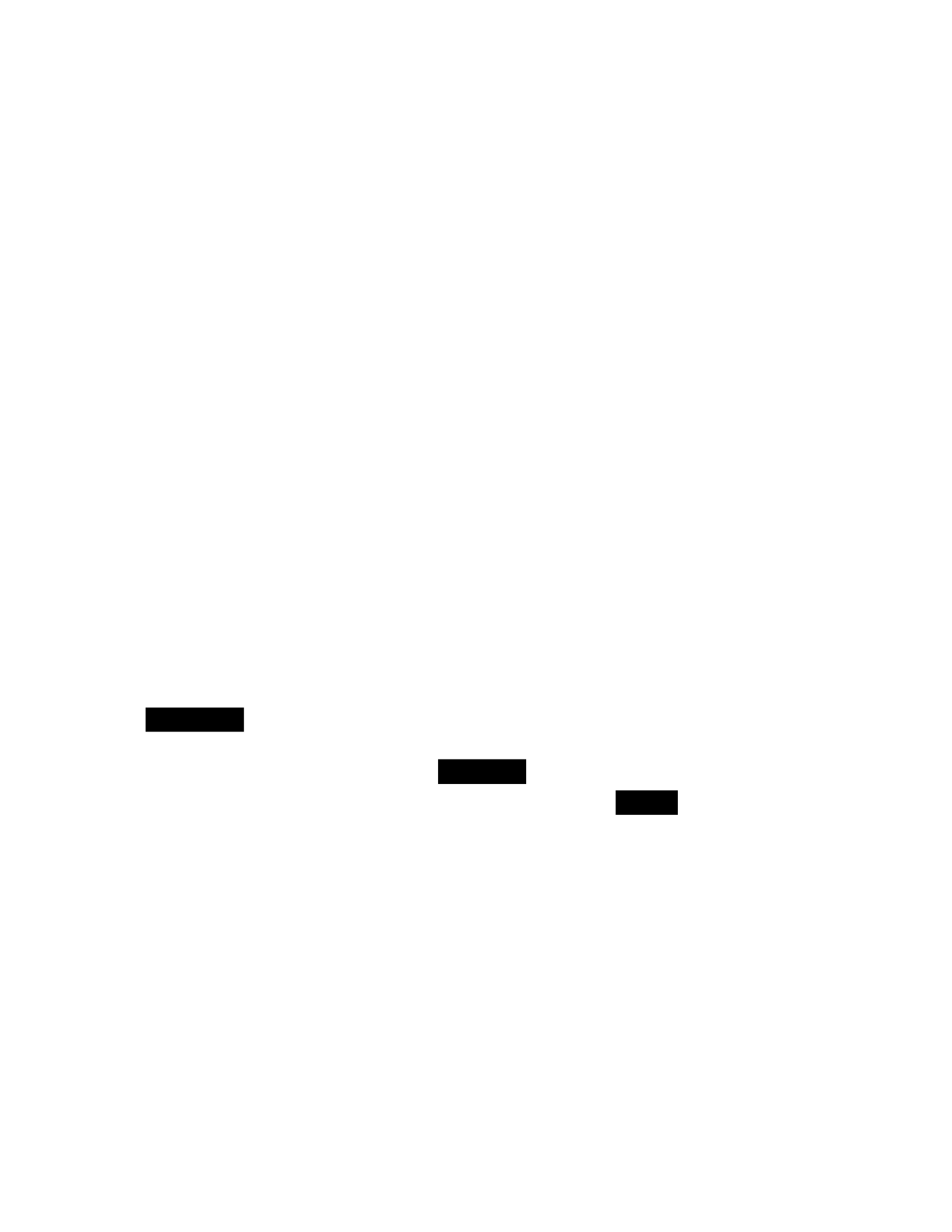
they are parasitic on a prior, unexplained concept of probability or expected

value. So I will give a brief argument to justify that real-valued proportions are

sensible as frequency judgments.

The intuition is this. Consider someone who can give integer-valued

estimates of the number of successes over n trials, for arbitrary n. We ask him

for his estimate of the number of successes over a single trial, and he tells us

either 0 or 1. Now we ask him, “if you repeated that single trial 10 times, then

averaged the number of successes over the 10 repetitions, what would you

estimate the average to be?” Because epistemic independence implies that there

is no difference between a 10-trial block and 10 1-trial blocks, he should give us

his estimate of the number of successes over 10 trials, divided by 10: this will be

the first decimal digit of his real-valued frequency judgment. We can continue

this process to elicit more digits, or we can simply ask him to “tell us the

averages first,” rather than bothering with the integer estimates. Formally:

Definition 2. Given an event E and a reference class R for it, an agent A’s frequency

judgment scheme for E is a map f : N → R, such that f(n) is a subjective estimate of

the number of times E will occur over n epistemically independent trials of R.

Evidently, f(n) [0∈,n] for every n.

So at this point, we are considering both frequency judgments in the original

sense, but also schemes that make integer predictions for every n. But now we

impose another criterion: f should be invariant under averaging. In other words,

let us say that f estimates that if we do n trials, we will have s successes. We

should also estimate that if we do 2n trials and then divide the number of

successes by 2, we should get s. In other words, we should have

In general, for any a ∈N, our estimate should be invariant under averaging

over a repetitions of the trial, i.e., ). But this implies that f should

satisfy f(an) = af(n) for any a ∈N. Now, fix some n and let ; clearly p is a

real number in [0,1]. For any m ∈N, nf(m) = f(mn) = mf(n) = mpn. Dividing by n,

we get that f(m) = pm for all m. We have shown that frequency judgment

schemes that are invariant under averaging are necessarily frequency

judgments, i.e., real-valued proportions.

Mathematically speaking, this argument is trivial; its significance is that we

appealed only to a notion of averaging over arbitrary repetitions, without any

circular appeal to probability or expected value. Furthermore, I think this

argument yields two important clarifications of the idea of frequency judgment:

1. The concept of invariance under averaging gives rise to a simple notion of

“long-run relative frequency” without appealing to an infinite sequence of

trials. Thus the frequency judgments interpretation appropriates some of

the benefits of hypothetical frequentism as analyzed by Ha´jek, without

having to carry any of its metaphysical baggage.

2. If f is invariant under averaging, then f(n) = nf(1). Thus, in some sense f

“views” every individual trial as contributing a fractional success f(1) ∈

[0,1] to the total estimate of successes. This is what justifies modeling

events that admit a frequency judgment as I.I.D. Bernoulli trials.

A concern remains: why is it sensible for p to take on irrational values? The

key is that the reals are Archimedean, i.e., for any two reals r1,r2, we have |r1 − r2|

> q for some rational q. It follows that over a sufficiently large integer number of

trials, any two distinct reals constitute distinguishable frequency judgments;

their estimates of the number of successes will vary by at least one whole trial.

For example, consider the irrational-valued frequency judgment 785398. Is

this judgment identifiable with any rational-valued approximation of it, e.g.,

.785? It is not, because over 100000 trials, they predict quite different things.

At this point, one might take issue with the idea that arbitrary-precision real

numbers are distinguishable in this way. Surely, at some point, the number of

trials required to make the distinction is so large that the heat death of the

universe will come first? I appreciate this concern, but I don’t think it’s specific

to probability — it seems akin to the idea that instead of modeling time as real-

valued quantities of seconds, we should model it as integer multiples of the

Planck time. There may be a bound on the resolution of reality, but it is

methodologically convenient to represent it as unbounded.

3.5 Characteristics of frequency judgments

Caveats

It is problematic to claim that frequency judgments are in fact a frequency

interpretation of probability, and I do not wish to paper over the difficulties. This

conception is a substantial retreat from the classical frequentism of Reichenbach

and von Mises. In particular:

1. A frequency judgment is not “made by the world”; it is not directly

derivable fromany actual past history of trials (as in the case of finite

frequentism), the past and future history of the world (as in some cases of

Lewis’s supervenience account), or any objective or universal conception

of an idealized hypothetical sequence of trials (as in the analogous case of

hypothetical frequentism).

2. A frequency judgment is explicitly relative to both an agent, because it is a

subjective estimate, and to a reference class. These relativizations may

look like reluctant concessions to realism, but in my opinion they are

features, not bugs — they capture essential indeterminacies that must be

part of any positivist account of probability. I will say more about both

relativizations below.

3. A frequency judgment need not pertain to events that are truly “random”

in any sense.Deterministic phenomena that are too difficult to analyze with

deterministic methods (such as the operation of a pseudorandom number

generator), when analyzed probabilistically, can be classed at this level of

the hierarchy. Thus, von Mises’s analysis of randomness by means of the

notion of Kollectiv (an idealized infinite random sequence with certain

desirable mathematical properties) is not relevant.

4. The notion of frequency judgment is intended as a conceptual analysis of

probability —it is an attempted elucidation of what is meant by statements

such as “the probability of flipping a U.S. quarter and getting heads is ,” or

“the probability of a Carbon14 atom decaying in 5715 years is .” It does

not follow from this that an agent’s frequency judgments are necessarily a

completed totality and form a σ-algebra obeying the Kolmogorov axioms.

A frequency judgment is not necessarily part of any global probability

distribution, even one relative to a particular agent; it is created by an act

of model-building and can be revised arbitrarily in ways that do not

correspond to conditional update.

How can frequency judgments be an interpretation of probability if they

do not straightforwardly obey the axioms? I think that the meaning of

probability is prior to the Kolmogorov formalization, and therefore that it

is legitimate for there to be some tension between the meaning and the

formalization — much as there is tension between the real number system

and the physical quantities whose measurements we represent as reals.

Frequency judgments can be used to build localized probabilistic models,

and each such model should obey the Kolmogorov axioms. Moreover, when

frequency judgments about the same event appear in different localized

models, they should ideally agree (although a lack of agreement does not

automatically prevent each model from being useful). But it is not essential

that there be meaningful global notions of an outcome space, an event

space satisfying the field axioms, etc. within which all frequency judgments

can coexist.

Relativization to reference classes

Frequency judgments are explicitly relativized to reference classes. Does this

mean that they cannot be an analysis of probability simpliciter? Concerning this

question, I endorse the argument by H´ajek [2007] that in fact, every

interpretation of probability is affected by a reference class problem, and thus

explicit relativization to reference classes is needed to dissolve an intrinsic

ambiguity.

I will briefly sketch Ha´jek’s argument as it applies to Bayesian subjective

probability. According to the most radical accounts of subjective credence, there

are no constraints on credence besides mere consistency. But intuitively, such a

view is unsatisfying because it does not enforce any kind of relationship

between one’s beliefs and reality. Ha´jek gives the following memorable

example:

The epistemology is so spectacularly permissive that it sanctions

opinions that we would normally call ridiculous. For example, you

may assign probability 0.999 to George Bush turning into a prairie

dog, provided that you assign 0.001 to this not being the case.

Thus it seems necessary to admit additional — external, evidence-based —

constraints on belief. Examples include Lewis’s Principal Principle, in which

beliefs must coincide with known chances, or Hacking’s Principle of Direct

Probability, in which they must coincide with observed relative frequencies. But

external “testimony” of this kind is, by its nature, subject to a reference class

problem. Consider the following case: John is 60 years old, a nonsmoker, and

previously worked with asbestos. We have statistics for the incidence of lung

cancer in 60-year-old nonsmokers and 60-year-olds with asbestos exposure, but

we have no statistically significant data concerning the intersection of those

groups. What should our credence be that John will develop lung cancer? We

might pick the first rate, or the second, or try to interpolate between them, but

implicit in any of these decisions is a statement about what reference class is to

be preferred.

Ha´jek’s conclusion from this analysis is that we need new foundations for

probability; he considers the true primitive notion of probability to be

conditional probability, where the assignment of the event to a reference class is

part of the proposition being conditioned on. That is to say, instead of

considering P(A), Ha´jek thinks we should be looking at P(A | A ∈R), where R is

a reference class. I think that the frequency judgments interpretation, in which

the reference class is part of the definition of (unconditional) probability, is a

more natural way of addressing this issue, and one that allows us to retain our

existing foundations. I discuss this question further in section 3.11.

Relativization to agents

The frequency judgments interpretation makes no reference to infinite

sequences or possible worlds; it relies only on the conceivability of performing

additional representative trials. Thus, its closest relative in terms of

metaphysical commitments is finite frequentism. But frequency judgments are

quite unlike finite frequencies in that they are agent-relative; two different

agents can have two different frequency judgments, even after they come to

agreement about a reference class. I will try to motivate this with a simple case

study. Consider the case of a coin that has been flipped 20 times and come up

heads 13 times. Is an agent constrained, on the basis of this data, to have any

particular estimate of the proportion of heads over a long sequence of trials?

Intuitively, the answer is no; a variety of beliefs about the coin’s long-run

behavior seem perfectly well justified on the basis of the data.

The ambiguities in estimation begin with the reference class problem. One

reading of finite frequentism is we must assign P(H) to be , the ratio of actual

successes to actual trials. This could be quite reasonable in some circumstances,

e.g., if the coin seems notably atypical in some way; however, to say that finite

frequentism requires this value is to do it an injustice. A finite frequentist might

also say that the reference class provided by the sample is deficient because of

its small size, and choose instead the reference class of all coinflips, yielding a

P(H) of , or rather, negligibly distant from . But the spectrum of choices does

not end there.

The maximum likelihood estimate of the probability of an event , the

ratio of successes to trials; this is a frequentist estimator in the sense that it does

not involve the use of prior probabilities. As such, it coincides with the first

reading of finite frequentism and estimates P(H) to be , but it would be a

mistake to identify the two perspectives. Rather, the maximum likelihood

estimate is the value of P(H) under which the observed data are most probable;

this is not an ontological attribution of probability but explicitly an estimate. As

such, it competes with Bayesian estimators such as the Laplace rule of

succession, which begins with a uniform prior distribution over the coin’s biases

and conditions repeatedly on each observed flip of the coin. The resulting

posterior distribution is the beta distribution β(s + 1,n − s + 1); to get the

estimate of the posterior probability, we take its expected value, which is

Since the rule of succession is derived from a uniform prior over the coin’s

biases, a different Bayesian might use a different prior. For example, using a

prior that clusters most of the probability mass around , such as β(n,n) for large

n, will produce an estimate arbitrarily close to . But on a different note entirely,

another frequentist might start with a null hypothesis that the coin is fair, i.e.,

, then compute the p-value of the observed data to be 0.26 and accept

the null hypothesis, retaining the estimate of .

None of these answers is prima facie unreasonable — even though they

differ considerably in methods and assumptions, they are all legitimate attempts

to answer the question, “if this coin is flipped a large number of times, what

proportion of the flips will be heads?” I am therefore rejecting Carnap’s

suggestion that there should in general be a best estimate of long-run frequency

from the data. We will have to live with a multiplicity of frequency judgments,

because room must be left for legitimate differences of opinion on the basis of

data.

Frequentism as a positivism

Given all this, why are frequency judgments still a frequency interpretation of

probability? I think they preserve the content of frequentism in two important

senses. First, their definition depends essentially on the notion of repeated trial.

If there is no conception of a reference class of trials, then there can be no

frequency judgment. Thus, the definition reflects the intuition that there is no

way to make frequentist sense of probability claims about one-off events.

More crucially, even though frequency judgments are not objective, they are

directly falsifiable from empirical data. Consider the example in the previous

section: on the basis of observing 13 heads over 20 trials, we considered a range

of different frequency judgments about P(H) to be valid. But no matter what

value we chose, we have a clear conception of how to further clarify the

question: we need to flip the coin more times and apply some statistical test that

can differentiate between the different judgments.

For example, consider the case of someone whose frequency judgment for

. If we go on to flip the coin 1000 times and get 484 heads, then (using

the normal approximation to the binomial) our observed result is 5.42 standard

deviations from the mean of 400 heads predicted by their hypothesis, which

yields a p-value on the order of 10−8. This is so highly improbable that we may

consider the frequency judgment of to have been falsified. This is not to say

that the much-maligned p-value test is the gold standard for the falsification of

frequency judgments; likelihood ratio tests can be used to achieve the same

results. If two agents can consense on a reference class for E, they can settle

whose frequency judgment for P(E) is correct. (See the appendix on more details

on how this consensus can be reached, in particular between a frequentist and a

Bayesian agent.)

This explains the intuition that frequency probabilities are objective. If there

is a large, robust body of trials for an event E (such as coin flipping), then any

frequency judgment that is not extremely close to the observed finite frequency

is already falsified. Thus, for events such as “a flipped U.S. quarter will land

heads”, our expected frequency judgment (in this case ) is very nearly objective.

How essential are repeated trials to this idea of probabilistic falsification?

Indeed, it is possible for a Bayesian probability for a one-off event to be falsified,

in the cases when that probability is very large or very small. For example, if an

agent makes the subjective probability assignment P(E) = .00001, and then E in

fact comes to pass, then the agent’s assignment has been falsified in much the

same sense as we discussed above. But if E is one-off, an credence like P(E) = 0.5

that is far away from any acceptable threshold of significance cannot be falsified.

The event E will either occur or fail to occur, but neither of these will be

statistically significant. Such a Bayesian credence lacks any empirical content.

In this sense, the definition of frequency judgment is an attempt to recover

the purely positivist content of frequentism. The metaphysical aspect of

frequentism, in which probabilities are inherently real and objective, has been

deferred to the level of chance. Inasmuch as Bayesian credences are purely

matters of personal opinion, without empirical content, they are also deferred to

another level.

3.6 Status of the frequentist-Bayesian debate

Frequency judgments and the error-statistical approach

At this point, it is appropriate to verify that despite the apparent concessions to

subjectivity in the definition of frequency judgments, they still preserve

essential elements of frequentism. In particular, can they properly distinguish

the probabilities used in frequentist statistical methods from the non-frequency

probabilities used in Bayesian methods? As it turns out, the frequency

judgments interpretation correctly interprets the frequentism of the

errorstatistical paradigm of statistical inference. A canonical example [Mayo and

Spanos, 2011] is classical significance testing. A p-value of .05 means we

estimate that if the null hypothesis were true and we repeated the experiment,

.05 of the experiments would exhibit results as extreme as the one observed.

This is straightforwardly a frequency judgment. Other methods utilizing test

statistics, such as chi-squared testing, follow this pattern; the test statistic is

computed from the data and then an estimate is given for the proportion of

experiments (given the null hypothesis) that would exhibit correspondingly

extreme values of the statistic. With confidence intervals, the frequency

judgment attaches to the procedure of deriving the interval: a 90% confidence

interval is associated with the estimate that if we repeatedly sampled and

computed the confidence interval, 90% of the resulting intervals would contain

the true value of the parameter.

In contrast, Bayesian methods in general allow the use of probabilities that

have no frequency interpretation. For example, a prior probability for a

hypothesis will not have one in general; rather it will represent epistemic

uncertainty about the truth of the hypothesis. Of course, there are settings in

which the prior in a Bayesian method may be interpretable as a frequency

judgment. Consider someone with three coins, with biases , who draws one

of‘ them at random from an urn, flips it 10 times, and observes 6 heads. The

agent can begin with a uniform prior distribution that assigns probability to

each coin, then use Bayes’ rule to obtain posterior probabilities as to which coin

he has. In this case, his prior is in fact a frequency judgment (“over a long

sequence of urn drawings, each coin will be drawn of the time”), and thus his

posteriors are also frequency judgments (“over a long sequence of drawing

coins from the urn and flipping them ten times, of the times I see 6 heads, ≈

0.558 of them will be because I drew the -coin”). But the method would be

equally applicable if the prior reflected only the agent’s subjective degrees of

belief in which coin he had.

Objectivity

My claim is that frequency judgments capture the objectively verifiable fragment

of probability — but not that they are actually objective, or are a prescription for

objectivity. As we have seen, data do not uniquely determine a frequency

judgment. Moreover, although frequency judgments are in principle subject to

probabilistic falsification, there is no objective threshold of evidence at which

this falsification takes place, and therefore there is no objective guarantee of

when it will occur in practice. Even after two agents with different frequency

judgments agree on a reference class of trials, it is possible for one or both of

them to insist on an unreasonably high evidentiary standard for the falsification

of their judgment. Moreover, this unreasonableness is interpretable in both

frequentist and Bayesian frameworks. For a frequentist, it might look like the

requirement of an unreasonable p-value (for example, p = 10− instead of the

more usual p = .05 or .01) to reject her initial frequency judgment. For a

Bayesian, it might look like a prior distribution placing an unreasonable amount

of probability mass on or near her initial frequency judgment.

Instead, the proposed distinction is this: frequency judgments are the only

case for probability in which we have a clear method of settling questions about

the accuracy of a fractional-valued probability. This is because the only thing

that can fix the value of such a probability is a frequency. This will become

important when considering how the frequency judgments interpretation

applies to problem cases for Bayesian credence, such as Sleeping Beauty

(section 3.11) and White’s Coin Puzzle (section 3.11).

Calibration

To remedy this, the literature on Bayesianism proposes the notion of calibration:

a Bayesian agent is calibrated if of the events he assigns credence to come to

pass, and so on.6 Calibration does seem to restore empirical content to single-

case subjective probability assertions — intuitively, given a one-off event E, a

subjective declaration that is more empirically justified coming from

an agent with a strong history of calibration than from one without one. The

problem is that calibration, as a norm on subjective agents, represents a

substantial compromise of the Bayesian view, so much so that it cannot be taken

to save the original notion of subjective probability from these criticisms.

Firstly, as Seidenfeld [1985] observes, calibration is straightforwardly

dependent on a notion of frequency probability, and what that notion is requires

explication. In what sense are we to interpret the statement that of the events

will come to pass? Seidenfeld considers finite-frequentist (“ of these events

have historically come to pass”) and hypotheticalfrequentist (“the long-run

relative frequency of these events coming to pass is ”) readings of this claim and

rejects them, for reasons akin to the difficulties Ha´jek sees with these

interpretations in general.

Can we make sense of calibration under the tiered interpretation? In fact, an

assertion of calibration has a straightforward interpretation as a frequency

judgment: the agent is taking the class of events she assigns subjective

probability to be a reference class, and then making a frequency judgment of

for that class. This is an empirical assertion, subject to confirmation or

disconfirmation in the manner discussed in the previous section. However, this

notion of confirmation is a property not of the single case, but of the class of

predictions as a whole. Just as before, any individual event E will either occur or

not occur, but neither validates the prediction until the occurrence or

non-occurrence of other, separate events is considered.

Secondly, just as calibration inherits the problems of definition that affect

frequency probability, it also inherits a reference class problem. For example,

van Fraassen [1983] gives the following surefire technique to achieve

calibration: make 10 predictions, on any subject, with probability . Then, roll a

fair die 1000 times, predicting an outcome of 1 each time with probability . At

the end of this, you will (with high objective probability) be calibrated, in the

sense that almost exactly of your predictions with probability will have come

true. But clearly your ability to make calibrated predictions about the die says

nothing about your predictive ability in general — it is unreasonable to place the

original 10 predictions and the subsequent 1000 in the same reference class.

To combine both of these objections, recall that we characterized frequency

judgments as capturing precisely the cases in which probability assertions were

subject to falsification. Does the notion of calibration successfully extend this to

all cases? It does not. Let E be a single-case event, to which Alice assigns PA(E) =

0.95 and Bob PB(E) = 0.05. Whether E occurs or fails to occur, both are perfectly

consistent with both Alice and Bob being calibrated. It is sufficient for Alice to

predict PA(Ai) = 0.95 for a sequence of events Ai of her choice having relative

frequency of success 0.95, and for Bob to do likewise for a different sequence of

events Bi of his choice. And the form of this disagreement is precisely that of a

reference class ambiguity — Alice classes E with the Ai, and Bob classes E with

the Bi, and their predictions are vindicated exactly inasmuch as those decisions

are accepted.

All of these difficulties have a common theme: calibration, as a norm,

entangles individual subjective probability assertions with the facts about a

larger class of events. Thus it cannot be taken to provide empirical content for

single-case probability assertions. And inasmuch as this empirical content does

in fact exist, my claim is that it is captured exactly by the notion of frequency

judgment: it is no more and no less than the ability to define an arbitrary

reference class and make a relative frequency assertion about it.

Convergence theorems

Now is the time to discuss a common argument in defense of Bayesian

probabilities: the existence of convergence theorems that demonstrate the

“swamping of priors” in the face of shared evidence. These theorems use

different hypotheses to reach different conclusions, but the common theme is

that they show that agents with different subjective prior distributions will

converge on the same subjective posterior distribution, given a suitable stream

of shared evidence. Thus, the apparent subjectivity of Bayesian probability is

only “temporary”, and in the long run Bayesian probabilities enjoy the same

claim to objectivity as frequency probabilities.

My reading of the convergence results surveyed by Earman [1992] is that

they fall into three categories. In the first category, we have results showing that

given a long sequence of i.i.d. trials of an event E, Bayesian agents beginning with

different priors will all converge on the same posterior probability for E, which

will also be the limiting relative frequency of E. As I see it, results of this kind (I

conjecture one in the appendix) support the privileged status of frequency

probabilities, rather than undermining it; it is precisely because E can be

subjected to repeated trial that the agents can come to agree about it. These

theorems are straightforwardly inapplicable to Bayesian probabilities for purely

single-case events E.

A second category is exemplified by the likelihood ratio convergence

theorem (LRTC) proven by Hawthorne [2011]. Results of this kind show that

Bayesian agents beginning with different priors for a hypothesis H will converge

on the same extremal-valued (0 or 1) posterior probabilities for H — that is to

say, come to agree about its truth or falsehood— as long as they are given a

shared stream of differentiating evidence in the form of likelihoods, which are

probabilities of the form P(E | H), i.e., probabilities of observing evidence given

the truth of the hypothesis. Thus, these results form the foundation of Bayesian

confirmation theory as an account of scientific progress — they purportedly

allow us to understand the empirical confirmation and disconfirmation of

scientific hypotheses as the convergence of Bayesian posterior probabilities.

At first blush, these results challenge the exclusive claim of frequency

judgments to objectivity — consensus is reached about P(H) even if no reference

class of trials can be associated with the hypothesis H. However, upon further

inspection, the import of the challenge is diminished. First, it should be noted

that the fractional-valued prior probabilities (e.g., P(H) = .15) are not actually

confirmed or disconfirmed themselves; they are merely stepping-stones to

integer-valued posterior probabilities representing truth or falsehood (e.g., P(H)

= 0). In this sense, the theorems only show agreement for the kind of

probabilities that Carnap would call Probability1, as opposed to Probability2.

Furthermore, these results leave the following question unanswered: why

should the agents agree about the likelihoods? As Hawthorne points out, it is in

fact a typical feature of scientific discourse that scientists agree on the evidential

import of experimental results. But we can distinguish two sources for these

shared (Hawthorne calls them “intersubjective”) likelihoods. One possible

source is from statistical analysis of experimental data, in which case the

likelihoods have a frequency interpretation — they are the frequency of

observing the data E when repeating the experiment, assuming that the

hypothesis H is true. In this case, the objectivity can again be seen to originate in

a frequency judgment. The other possibility is that rather than originating in

statistics, they represent subjective appraisals of the evidentiary value of data —

one of Hawthorne’s examples is how the similarity between the coastlines of

Africa and South America confirms the theory of continental drift. In cases such

as this, I consider that Bayesian probability does nothing to explain why

different agents should agree, even approximately, on any quantification of the

evidentiary value. The invocation of “likelihood” in cases like this seems to me to

be only a metaphor for the strength of evidence, having little to do with the

corresponding statistical notion. In this sense, Bayesian confirmation theory

does not improve on non-quantitative accounts of scientific consensus, e.g., “a

scientific hypothesis is accepted once it is favored by a preponderance of

evidence.”

Finally, Earman describes convergence theorems based on Doob’s martingale

convergence theorem, which similarly show convergence to integer-valued

posterior probabilities, but without even the requirement of shared likelihoods.

Instead, the accumulation of shared evidence is represented through the

technical device of an increasing filtration over the probability space of events.

As in the previous case, I consider that the burden is on Bayesians to say exactly

what kind of shared evidence, if not frequency probability, this abstraction is

modeling. Until this is specified, the import of these theorems is metaphorical

rather than substantive.

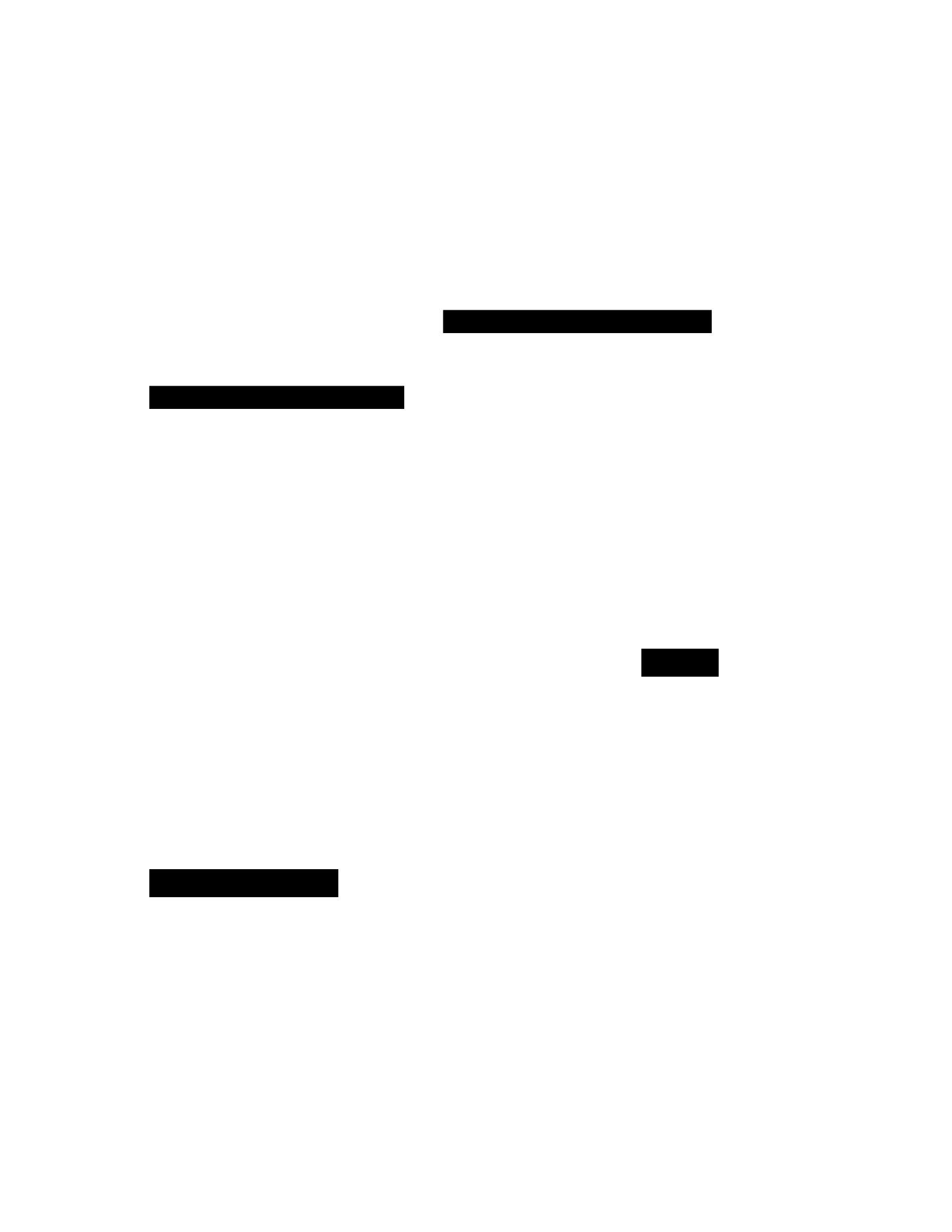
The likelihood principle

In the previous section, I claimed that likelihoods are frequency probabilities of

the form P(E | H). But this is is not always strictly true — and the cases in which

it isn’t are at the core of a significant controversy in the philosophy of statistics,

namely the debate over the likelihood principle. Consider the following case

[Royall, 2004]: a coin is flipped 20 times and we observe 13 heads. Let H θbe the

hypothesis that the coin’s bias is θ, for some 0 ≤ θ≤ 1. What is P(E | Hθ)? Over

the reference class of trials of the form “flip a coin 20 times”, the frequency

probability of observing 13 heads is . But over

the reference class of trials of the form “flip a coin repeatedly until 13 heads are

observed”, the frequency probability of having to do 20 trials is

. It follows that a large class of error-statistical

methods that work directly with P(E | Hθ), including p-value testing and

confidence intervals, cannot interpret the data until it is decided which

reference class to use — and the decision has the potential to change statistical

insignificance into significance or vice versa. Another way to put it is that the

interpretation of the data depends on a counterfactual question about the

experimental procedure: if the experimenter had observed 13 heads over 18

flips, would she have stopped or continued flipping?

The intuition that these considerations should be irrelevant to the evidential

meaning of the observation itself — which seems to consist simply of the 13

heads and the 7 tails — motivates the use of likelihood-ratio testing to interpret

the data. In particular, given two candidate biases θand is well-

defined independently of the procedure that generated E, because the constant

factor divides out out of the expression. This also motivates the idea that the

evidence is summarized by the function θ13(1 − θ)7, that is to say, P(E | Hθ) up to

a constant factor. This is called the likelihood function. The likelihood principle

states that the likelihood function must be a complete description of the

evidence. As discussed previously, likelihood-ratio testing satisfies the principle

while p-value testing violates it. Moreover, a wide class of Bayesian methods

satisfy the principle — intuitively, because Bayesians are interested in

, and when P(E) is expanded as a sum over alternate

hypotheses P

H′ P(E | H′), any constant factor associated with P(E | H) divides out

of the expression. Thus, the intuitive plausibility of the likelihood principle is

sometimes advanced as a justification for the use of Bayesian, as opposed to

classical, statistics. Meanwhile, some frequentists (notably Mayo [2010]) reject

the likelihood principle, and a small group of likelihoodists (notably Royall

[2004]) support methods which satisfy the principle, but which are non-

Bayesian in the sense that they do not make use of prior distributions.

Does the frequency judgments interpretation imply a commitment to

frequencies over likelihoods, and thus the denial of the likelihood principle? My

hope is that it succeeds in remaining agnostic about the question. Likelihoods

have evidential import precisely because they are informative about frequencies

— frequency probabilities are directly proportional to likelihoods, and ratios of

likelihoods are ratios of frequencies.

3.7 The third tier: Bayesian probability

I will use the term “probabilism” to describe the following view:

1. Uncertain knowledge and belief can (at least some of the time) be modeled

by probabilities (“credences”, “Bayesian personal probabilities”).

2. These credences can (at least some of the time) be measured by an agent’s

dispositionto act or bet.

3. Credences ideally satisfy the Kolmogorov axioms of probabilistic

consistency.

4. The desirability of this consistency is demonstrated by the Dutch Book

argument.

According to this definition, I consider myself a probabilist. It seems perverse

to me to try and dispense entirely with the idea of real-valued credence — at the

very least, I really do have propensities to bet on a variety of uncertain events

that have no frequency interpretation, and Bayesian subjective probability can

assist me in pricing those bets. Moreover, inasmuch as there is any kind of

precision to my uncertain knowledge and belief, I am more sympathetic to

classical probabilism as a representation of that uncertainty than I am to other

formal techniques in knowledge representation, for example the AGM axioms.

And it seems to me that this system provides the most natural resolution of

various problems related to partial belief, such as the preface paradox. Hence

the three-tiered interpretation accords a place to Bayesian credences, defined in

the standard way according to the Bayesian literature.

By contrast, I will use the term “Bayesian subjectivism” to denote the

following expansion of the view:

1. An agent has at all times credences for all uncertain propositions,

representing implicitdispositions to act, and forming a completed σ-

algebra that is consistent according to the Kolmogorov axioms of

probability.

2. All knowledge can be assimilated to this framework, and all learning can

be describedas conditional update.

I disagree intensely with this view. As a frequentist, I am perpetually

surprised by the insistence of Bayesian authors that I have credences for

propositions I have never considered, that I should elevate my unfounded

hunches and gut instincts to the level of formalized belief, or that I should apply

the principle of indifference and believe completely uncertain propositions to

degree . When confronted with dispositional or gambling analyses, which allege

that my credence can be measured by my propensity to bet, my response is that

there are many propositions on which I would simply refuse to bet, or deny that

I have a precise indifference price for a bet. And indeed, the rationality of this

response is being defended increasingly in the literature, under the heading of

“imprecise” or “unsharp” credence — see Elga [2010] or Joyce [2010] for

arguments that there are situations in which precise credences are unobtainable

or unjustifiable.

Nor is the difficulty of eliciting precise credences the only foundational

difficulty with the Bayesian view. The intuition that Bayesian subjectivism as an

account of all uncertain reasoning represents an inherently unfeasible ideal,

even at the aspirational level, is supported by both philosophical and

mathematical evidence. Examples include Garber’s observation [1983] that

taking the position literally implies the existence of a unified language for all of

science (the project the logical positivists failed to complete), or Paris’s proof

[1994] that testing probabilistic beliefs for consistency is NP-complete.

However, as in the case of physical chance, a variety of conceptions of

Bayesian probability are enabled by the three-tiered interpretation. In

particular, if you are a traditional Bayesian, then you have Bayesian credences

for a very wide range of propositions. Some of your credences also happen to be

frequency judgments, and some of those in turn happen to be chances, but these

distinctions are not of central importance to you. But the threetiered view also

enables a much more skeptical attitude to Bayesian probability, one that is

identifiable with the skepticism of traditional frequentism: credences that have

frequency interpretations can take on definite values while credences that have

no such interpretation are unsharp or remain in a state of suspended judgment.

3.8 The transfer principles

I claimed that probabilities from the first tier transfer to the second, and from

the second to the third, the conjunction of these constituting a fragment of the

Principal Principle. However, I suspect that no one will be especially interested

in contesting this aspect of my argument — Bayesians already endorse the

Principal Principle, and frequentists find it perfectly acceptable to bet according

to frequency ratios. So the purpose of my discussion will be as much to clarify

the underlying notions as to prove the principles.

Claim 1. Let E be an event. If an agent can assign E to a reference class R, she

knows a physical chance p for events in the class R, and she has no other relevant

information, she is obliged to have a frequency judgment of p for E and R.

This is more or less trivial. If we know that a class of events exhibits chance,

then we can model sequences of those events as I.I.D. draws from the relevant

distribution.

Claim 2. Let E be an event. If an agent has a frequency judgment p for E (by virtue

of associating it with an unambiguous reference class R), and no other relevant

information, he is obliged to have a Bayesian subjective probability of p for E.

The argument for this is as follows: let the agent consider how to buy and sell

bets for a sequence of n events in the reference class R, for n arbitrarily large. He

estimates that a proportion p of these events will come true. Therefore, the fair

price for the sequence of bets is pn; any higher and if he buys the bets at that

price, he will lose money according to his estimate, any lower and he will lose

money by selling them. But since R is epistemically homogeneous for the agent,

and in particular he has no information that distinguishes E from the other

events, each individual bet must have the same price. Thus, his fair price for

a bet on . □

This argument should not be taken too literally, since it neglects (among

other decisiontheoretic issues) the possibility of nonlinear utility in money.

Rather, it illustrates the relationship between frequency judgments and Bayesian

credences within some “normal domain of applicability” for the latter, in which

credence and betting behavior do not significantly come apart. It might be more

accurate to say that inasmuch as the agent can be said to have a degree of belief

in E — and, as Eriksson and H´ajek [2007] show, the precise meaning of this is

remarkably difficult to pin down — it should be p. However, in a behavioral or

decision-theoretic sense, this should not obligate the agent to maximize

expected value or utility with respect to p, rather the agent should be at liberty

to be risk-averse, or even to act according to a worst-case rule such as

maximinimization.

How much of the Principal Principle have we recovered? We have it for any

event that has a chance and belongs to a reference class. This captures most

conventional uses of PP, for example the radioactive decay of atoms (even

Unobtainium). But we have seemingly failed to recover it in the case of one-off

events. For example, what happens when we have come to understand an

inherently unique macrophysical phenomenon as possessing a chance of p? We

cannot have a frequency judgment about it, so on the basis of the reasoning here

we are not constrained to have a credence of p in it.

This is a genuine problem and I cannot resolve it entirely here — a solution

would seemingly require a detailed analysis of the meaning of chance. As a last

resort I can simply defer to an existing justification of PP that doesn’t go through

frequency judgments. But here is a brief sketch in defense of the full PP on the

basis of the frequency judgments view. PP is inherently a principle of

epistemology, not metaphysics, because it describes a constraint on credences

(which are necessarily an epistemic notion). Therefore it is appropriate to ask

how we would actually come to know the value of this one-off macrophysical

chance — we couldn’t have learned it from observed frequency data. The most

natural answer seems to be that we would learn it via a theoretical model in

which the overall macrophysical chance supervened on microphysical chances.

And then this model would provide the basis for a frequency interpretation of

the chance: over the reference class of situations satisfying the initial conditions

of the model, the desired event would come to pass in some proportion p of the

situations. This doesn’t exhaust all possible methods by which we could come to

know p, but I hope it fills in a good portion of the gap.

Finally, notice the qualifications in the second principle: the reference class

must be unambiguous, and there must be no other relevant information. The

second of these requirements corresponds to the requirement of admissibility

commonly associated with the Principal Principle; if you have information about

an individual event that informs you about it beyond the background chance of

success or failure, then PP is not applicable. (A simple example: you are playing

poker and your opponent is trying to complete a flush. You know that the

objective chance of this occurring is low, but you have seen him exhibit a “tell”,

for example, the widening of the eyes in excitement. Your credence that he has a

flush should increase to a value higher than that dictated by the PP.) There is a

sophisticated literature on when exactly PP is admissible, and I have no

particular stance on the issue. Indeed, my view is that both qualifications are

features and not bugs. When admissibility is debatable or the reference class is

ambiguous, there is no fact of the matter about what should be believed.

3.9 Populations, direct inference, and the Principle

of Indifference

White [2009] calls the second transfer principle “Frequency-Credence”. He

claims that it implies the generalized Principle of Indifference, i.e., the rule that if

you are faced with n mutually exclusive alternatives and have no information to

distinguish them, you should assume a credence of for each one. An especially

revealing case is an individual proposition q concerning which you have no

relevant information: since exactly one of {q,¬q} is true, the Principle of

Indifference indicates that you should assign P(q) = P(¬q) = 0.5. Such a principle

is of course anathema to frequentists, since it is applicable in cases when there is

no possible frequency interpretation of P(q). Thus, White’s purpose is to show

that frequentist squeamishness about the Principle of Indifference is incoherent.

Here is his statement of Frequency-Credence:

Claim 3. If (i) I know that a is an F, (ii) I know that freq(G | F) = x (the proportion

of Fs that are G), and (iii) I have no further evidence bearing on whether a is a G,

then P(a is a G) = x.

and here is his proof ( denoting epistemic indistinguishability):≃

Let F = {p1,p2,...,pn} be any set of disjoint and exhaustive

possibilities such that p1 ≃p2 ≃...pn. Let G be the set of true

propositions. For any pi, (i) I know that pi is an F; (ii) I know that freq

(exactly one member of the partition {p1,p2,...pn} is true);

and (iii) I have no further evidence bearing on whether pi is G (I am

ignorant concerning the pi, with no reason to suppose that one is

true rather than another). Hence by FC, P(pi is a , i.e.,

P(pi is true) = , so . □

White challenges opponents of the Principle of Indifference to identify a

restriction of Frequency-Credence that disallows this proof. Fortunately, the

frequency judgments interpretation and the second transfer principle qualify as

just such a restriction. Moreover, the precise way in which they block the

conclusion reveals some interesting information.

Everything hangs on the following assertion in the proof: that freq .

For

White, this is just the observation that exactly one of the possibilities p1 ...pn is

true, i.e., it is the finite frequency of true propositions among the available

possibilities. But for the second transfer principle to apply, this must constitute a

genuine frequency judgment, and without a reference class and a conception of

repeated trial, a frequency judgment cannot exist. In particular, if the

alternatives are q and ¬q for a single-case proposition q with no obvious notion

of trial (“God exists”, “Chilperic I of France reigned before Charibert I”), no

frequency judgment will be supported, and there is no obligation to set P(q) =

P(¬q) = 0.5; rather it is perfectly reasonable to be in a state of suspended

judgment, or to have an unsharp credence interval.

There is a subtlety here because the principle of indifference can indeed be a

source of legitimate frequency judgments. If for some genuine reference class of

repeated trials, each trial has the same n mutually exclusive outcomes, then it

can be perfectly legitimate to estimate a priori the long-run frequency of each

one as This estimation may not be justified or accurate, but that doesn’t

matter; as discussed previously, what matters is the possibility of confirming or

disconfirming the judgment from empirical data. But even in this case, we do not

recover the principle of indifference as an obligation, merely as an option. There

is no obligation to formulate frequency judgments in the absence of evidence —

dispositional betting arguments try to elicit credences in this way, but obviously

this doesn’t go through for frequency judgments.

Direct inference

There is another subtlety: observed finite frequencies are not necessarily

frequency judgments! Consider the following scenario, discussed by Levi [1977]

and Kyburg [1977]: of the 8.3 million Swedes, 90% of them are Protestants.

Petersen is a Swede. What should our credence be that Petersen is a Protestant?

Intuitively, there seems to be a frequency probability that P(Petersen is a

Protestant) = 0.9. Arguments of this form — going from relative frequency in a

population to a credence — are called direct inferences or statistical syllogisms,

and they are a significant aspect of our probabilistic reasoning. But if we try to

phrase this as a frequency judgment, we encounter problems. The Swedes are

not a reference class of events, and there is no obvious notion of repeated trial at

work.

The situation seems analogous to the case of {q,¬q}. The intuition that we

should have a credence of 0.9 is seemingly grounded in the idea that Petersen is

one of the 8.3 million Swedes, and we are indifferent as to which one he is. But if

we allow unrestricted reasoning of this kind, then it will apply to the two

propositions {q,¬q} as well, and White’s challenge will succeed after all — we

will have conceded that making use of frequency probabilities implies a

generalized principle of indifference. Can we save the intuition that P(Petersen

is a Protestant) = 0.9 without conceding P(q) = P(¬q) = 0.5?

Here is a case that may clarify what the frequency judgments interpretation

says about this kind of reasoning. You are a contestant on a game show; a prize

is behind exactly one of three closed doors, and you must choose which one to

open. What should your credence be that the prize is behind the left door?

Whatever this credence is, if it is to be associated with a frequency judgment, it

must be possible to clarify it with respect to the long-run behavior of repeated

trials. The natural conception of repeated trial here is that we would play the

game repeatedly and measure the proportion of times that the prize is behind

the left door.

11In a Bayesian framework, this would be an uninformative prior, or indifference prior, over

the n alternatives.

And it is not clear that any particular frequency judgment is supported about

this reference class of trials — we might imagine that the show host has a bias

towards one of the doors in particular. Considerations like this support a view in

which your credence that the prize is behind the left door is indeterminate or

unsharp, or in which you suspend judgment about the question. Contrast this

with the following claim: if you flip a fair coin with three sides and use the result

to decide which door to choose, you have a frequency judgment of that this

procedure will yield the correct door, regardless of any bias the host might have.

In this case, a frequency judgment is fully supported, because the reference class

is clear (flips of the coin) and its properties are unambiguous, and there is a

convincing case that the second transfer principle obligates you to have a

credence of .

However, it seems natural that we should wish the credence of to be

available at least as an option for the rational agent faced with the original

problem, and to be able to make sense of this under the frequency judgments

interpretation. I think this is possible via the following expedient: we construct a

model of the show in which the host selects the prize door via a coin flip.

Acknowledging that this model, like any model, may not be true, we can use it to

support a frequency judgment of for each door. Returning to our original

problem, we can adopt a model in which the process by which we encounter

Swedes is a chance process, analogous to a lottery in which we are equally likely

to draw any individual Swede. This model then supports a frequency judgment

of .9 for Protestants and a credence of .9 that Petersen is one.

This technique — modeling unknown processes as chance processes — is

the general idea of how direct inference is supported under the frequency

judgments interpretation. Does it, as White alleges, imply a generalized principle

of indifference? As discussed above, even when the technique is applicable, it is

not obligatory; the option of suspending judgment (or having an unsharp

credence) is left open. Moreover, the technique seems to get at an important

distinction between two kinds of indifference. It applies straightforwardly to

situations where one is indifferent between individuals (prize doors, Swedes),

but not to situations where one is indifferent between propositions (which king

reigned first). Indeed, to interpret the second kind of indifference within our

framework, we would seemingly have to talk about an indifference between

possible worlds, and of a chance process deciding which one we live in. At this

point we have regressed to the kind of reasoning decried by C. S. Peirce, of

imagining that “universes [are] as plenty as blackberries” and we can “put a

quantity of them in a bag, shake well them up, [and] draw out a sample.” This

kind of reasoning is not frequentist and therefore it is appropriate that we

cannot understand it on frequentist terms.

3.10 H´ajek’s objections to frequentism

As I understand the frequency judgments interpretation, it avoids the bulk of H

´ajek’s objections simply by failing to be a frequentism in the classical sense of

the term. Let F.n denote his nth objection to finite frequentism, and H.n his nth

objection to hypothetical frequentism. It seems to me that most of his objections

are straightforwardly dismissed by one or more of the following concessions:

1. Not constraining frequency probabilities to be actual finite frequencies.

This obviatesobjections F.2, F.5, F.6, F.8, and F.12-15.

2. Not considering frequency probabilities to be determined by hypothetical

infinite sequences of trials. This obviates objections H.1-6, H.8-9, and H.13-

14.

3. Acknowledging the possible existence of physical chance. This answers

objections F.3,F.7, F.9, F.11, H.7, and H.10,

4. Acknowledging the legitimacy of Bayesian subjective probabilities. This

answers objections F.10 and H.10.

Of the remaining objections: H´ajek himself has subsequently repudiated F.1,

which criticizes finite frequentism on the grounds that it admits a reference

class problem. As discussed in section 3.5, H´ajek now considers the reference

class problem to affect every interpretation of probability, and I fully concur. I

take H.11 (which concerns paradoxes associated with uncountable event

spaces) to affect the Kolmogorov formalization of probability itself rather than

frequentism specifically. H.15, which says that frequency interpretations cannot

make sense of infinitesimal probabilities, I take to be a feature and not a bug.

The two remaining objections, F.4 and H.12, have a common theme — they

say that frequentism cannot make sense of propensity probabilities. This is a

serious issue that the three-tiered interpretation does not entirely address. In

particular, here is Ha´jek’s thought experiment from H.12:

Consider a man repeatedly throwing darts at a dartboard, who

can either hit or miss the bull’s eye. As he practices, he gets better;

his probability of a hit increases: P(hit on (n + 1)th trial) > P(hit on

nth trial). Hence, the trials are not identically distributed. [...] And he

remembers his successes and is fairly good at repeating them

immediately afterwards: P(hit on (n+1)th trial | hit on nth trial) >

P(hit on (n + 1)th trial). Hence, the trials are not independent.

Intuitively, all of these probability statements are meaningful, objective

statements about the properties of the man (or of the dart-throwing process as a

whole). Yet by their nature, we have difficulty in understanding them as

statements about relative frequencies over sequences of independent and

identically distributed trials. H´ajek is unimpressed with the reply that in order

to obtain a frequency interpretation of these probabilities, we should “freeze the

dartthrower’s skill level before a given throw” and then consider hypothetical

repeated throws by the frozen player. On one level, this notion of “freezing“

involves an appeal to a nonphysical counterfactual. On another, relative

frequencies seem irrelevant to the intuition that the thrower has, before each

throw, some single-case propensity to hit or miss the target. The intuition here is

analogous to the case of chance, except that there is no clear way to interpret the

dart-throwing system as subject to physical chance.

I can see no way for the three-tiered interpretation other than to resolutely

bite this bullet. That is to say, the three-tiered interpretation does not make

rigorous the idea of propensity probabilities that are not chances. For example,

consider the example in Levi [1977] of a glass bottle being struck with a

hammer. Intuitively, we can assign a fractional-valued probability to the event

“the bottle breaks into 10 pieces”, even though by definition the bottle can only

be struck once. However, the three-tiered interpretation can only interpret such

a probability in one of two ways. Firstly, it can be interpreted from the “top

down”, as a chance, by identifying the probability with a chance posited by an

underlying physical theory. As discussed in section 3.3, depending on one’s

preferred account of chance, this number may represent either a measurement

of physical indeterminism in the system, or it may merely be an indispensable

methodological posit. Alternately, the probability can be interpreted from the

“bottom up” as a frequency judgment, as a statement about what would happen

to the class of similar bottles when struck by similar hammers in similar ways. In

this I am agreeing with von Mises, who held that we cannot make sense of such

single-case assertions as “the probability that John will die in the next 5 years is

10%.”

In defense of this refusal with respect to Ha´jek’s dart-thrower, I can only say

this: the only way we were able to formulate this model in the first place was to

observe the behavior of multiple dart-throwers, and thus to reason about

reference classes of darts players in specific situations (e.g., immediately after

hitting the bulls-eye). Furthermore, how would we confirm the applicability of

this model to any specific player? It seems that we would do so via some sort of

calibration test — and, as discussed in section 3.6, calibration is always

implicitly or explicitly dependent on some notion of frequency probability.

3.11 Advantages of the tiered interpretation

Statistical pragmatism

As discussed in section 3.6 and subsequently, the frequency judgments

interpretation accurately describes the distinction made in traditional

frequentist statistics between the frequency probabilities that attach to trials

and procedures and the non-frequency probabilities that describe confirmation

of hypotheses. Thus, the three-tiered interpretation (with frequency judgments

as its middle tier) is a suitable foundation for statistical pragmatism [Senn,

2011], i.e., for a worldview in which frequentist and Bayesian methods coexist.

In order to admit the use of Bayesian methods, the three-tiered interpretation

acknowledges the existence of non-frequentist prior probabilities. But it also

formally distinguishes the probabilities used by properly frequentist methods

from those used by Bayesian methods; if it did not, frequentist methods would

appear simply to be peculiarly defective Bayesian methods. Methodologically,

the three-tiered interpretation is a reconciliation between the paradigms but not

a capitulation.

Cromwell’s rule

A notorious problem for subjectivist Bayesianism is the difficulty associated

with assigning probabilities of 0 or 1. Let’s say you assign P(A) = 0. Then for any

= 0, so you can never revise P(A) by conditioning on new

information. The case

for P(A) = 1 is analogous, as is the situation when standard conditionalization is

replaced by Jeffrey conditionalization.

Thus, according to many interpretations, a strict Bayesian should never

assign a probability of 0 to an event, no matter how unlikely; Lindley calls this

requirement Cromwell’s rule. But frequency judgments are not affected by this

problem, because they can be revised arbitrarily. Perhaps the clearest example is

the case of estimating the bias of a coin, where we admit a third event besides

heads and tails: it is physically possible that the coin might come to rest on its

edge, or that the outcome of the flip might remain undetermined in some other

way. A strict Bayesian is apparently committed to having prior probabilities for

all of these events — and fixing P(H) = P(T) = 0.5 entails a violation of

Cromwell’s rule, since no probability mass is left over for them. But under the

frequency judgments interpretation, there is no difficulty associated with

revising a probability from zero to a nonzero value.

Perhaps questions of this kind are artificial, unrelated to genuine concerns of

statistical practice? On the contrary, they seem to correspond to actual

methodological difficulties that arise when adopting a strictly Bayesian

perspective. Gelman and Shalizi [2012] describe how a rigidly Bayesian outlook

can be harmful in statistical practice. Since “fundamentally, the Bayesian agent is

limited by the fact that its beliefs always remain within the support of its prior

[i.e., the hypotheses to which the prior assigns nonzero probability]”, it is

difficult to make sense of processes like model checking or model revision, in

which a model can be judged inadequate on its own merits, even before a

suitable replacement has been found. They instead join Box [1980] and others in

advocating a picture where individual Bayesian models are subjected to a non-

Bayesian process of validation and revision. Dawid [1982], whose calibration

theorem suggests a similar difficulty with the Bayesian agent being able to

recognize his or her own fallibility, is led also to an endorsement of Box. The

point is not that these statisticians are betraying Bayesianism, it is that their

pragmatic interpretation of Bayesian statistical methodology bears little

resemblance to the worldview of the formal epistemologist who endorses

Bayesian confirmation theory.

Foundations of conditional probability

Bayesian probability proves its worth in dissolving paradoxes associated with

partial belief. Yet it is affected by its own set of paradoxes. I believe that the

tiered interpretation, in its capacity as a relaxation of strict Bayesian discipline,

can dissolve some of these as well — most notably, those in which Bayesian

conditionalization is expected to subsume all probabilistic model-building.

Ha´jek [2007] gives the following paradox. An urn has 90 red balls and 10

white balls. Intuitively, P(Joe draws a white ball from the urn | Joe draws a ball

from the urn) = .1. But in the standard Kolmogorov interpretation of probability,

conditional probability is not a primitive notion but a derived notion, so in order

for this statement to be true, we must have P(Joe draws a ball and it is white) /

P(Joe draws a ball) = .1. But neither one of these unconditional probabilities

appears well-defined on the basis of our assumptions. As H´ajek asks, “Who is

Joe anyway?”

Ha´jek’s solution is to suggest that conditional probability is the true

primitive notion and that we should consider alternate (non-Kolmogorov)

formulations of probability that elevate it to its rightful place as such. But this

seems to miss the mark. In particular, even though P(Joe draws a white ball | Joe

draws a ball) is well-defined, P(Joe draws a white ball | Bill flips a coin) is not.

Moreover, we can recover unconditional probability from conditional

probability, for example by conditioning on independent events (e.g., P(Joe

draws a white ball | a distant radium atom decays)) or on tautologies (e.g., P(Joe

draws a white ball | p ¬∨p)). It seems that conditionalization is orthogonal to

the true problem: when does a situation support a probabilistic analysis?

Under the tiered interpretation of probability, this problem is confronted

directly and admits a natural resolution. The fact that Joe is drawing a ball from

the urn provides enough information to support a model and a frequency

judgement: it calls into existence a probabilistic model in which we have an

extremely simple event space: “Joe draws a white ball” or “Joe draws a red ball”.

In this model, the value from our intuition appears as an unconditional

probability: P(Joe draws a white ball) = .1. Saying this is no more and no less

than saying that if Joe repeatedly draws balls from the urn with replacement, the

natural estimate of the proportion of white balls is .1. In general, the process of

assigning an event E to a reference class and then identifying P(E) with the

frequency judgment for that class is a more natural description of our

probabilistic model-building than a strict Bayesian conditioning view.

Ha´jek’s other paradox in the article, that of conditioning on events of

probability zero, admits a similar resolution. Ha´jek has us consider a random

variable X uniformly distributed on [0,1]. Intuitively, )

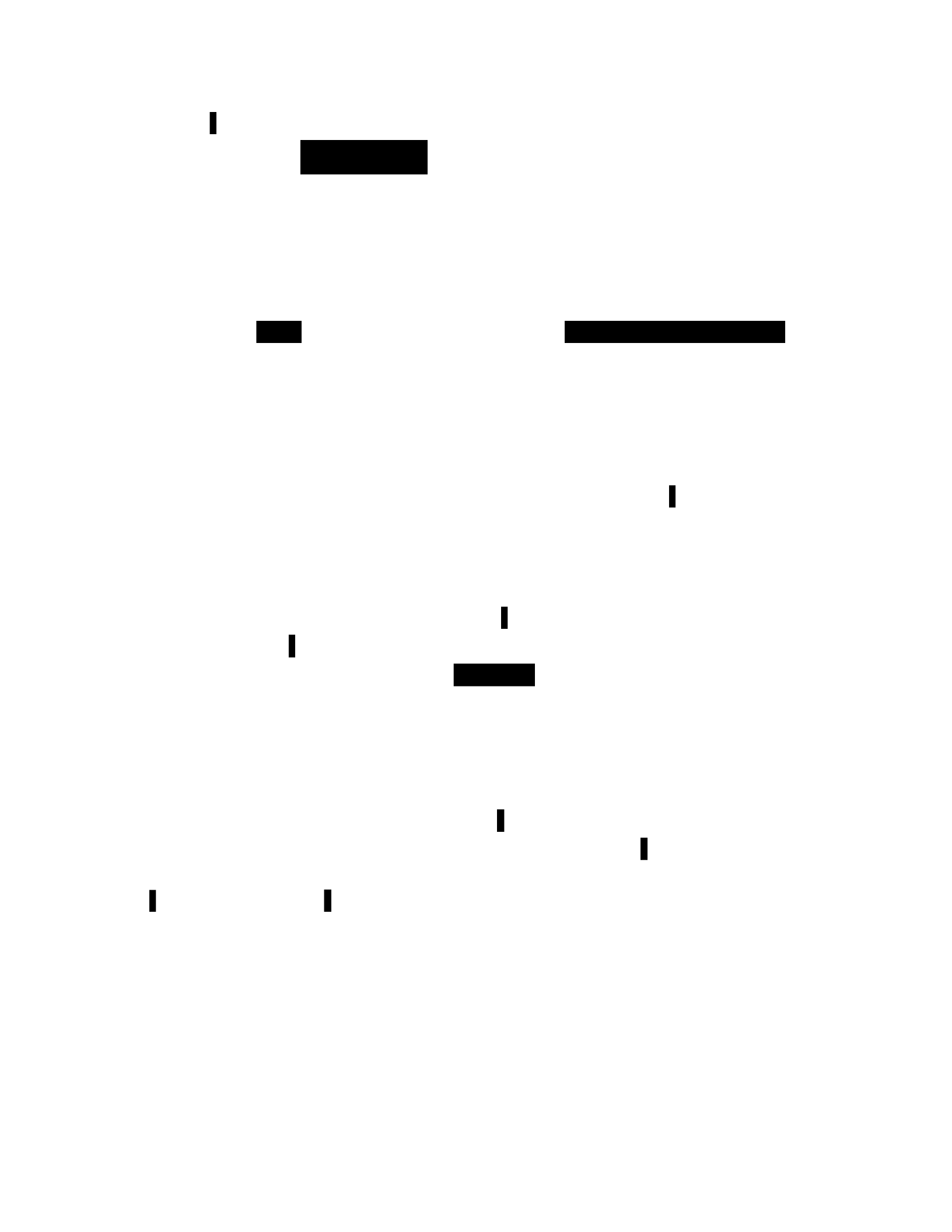
equals . But if we expand this using the standard definition of conditional

probability, we get , which is undefined.

Once again, the problem seems to be that we are taking an unnecessarily

narrow view of the model-building process. It is natural that we should try to

transform a continuous distribution into a discrete one by setting P(X = a) = f(a),

where f is the density function, and renormalizing — this has a natural

interpretation as the outcome of considering P(|X − a| < ϵ) for smaller and

smaller values of ϵ. When applied to H´ajek’s uniform distribution, with a

ranging over , this yields the expected answer .

It should not be considered problematic that this model transformation cannot

be interpreted as a conditional update.

Sleeping Beauty

The Sleeping Beauty Paradox, popularized by Elga [2000], goes as follows. A fair

coin, i.e., one that lands heads with an objective probability of , is flipped on

Sunday, and then Beauty is put to sleep. If it lands heads, Beauty is awakened on

Monday, interviewed, his memory is wiped and he is put back to sleep. If it lands

tails, this is done once on Monday and once on Tuesday. Beauty has just awoken.

What should his credence be that the coin landed heads? The “halfer” position is

that since the coin is fair, P(H) must equal . But if the experiment is repeated

many times, only of Beauty’s awakenings will be because the coin landed heads

— hence the “thirder” position that . Which of these is the correct

credence?

Sleeping Beauty is a vexing problem for Bayesian epistemologists and has

generated a rich literature. But, as Halpern [2004] observed, the paradox is

immediately dissolved by a frequentist analysis: it is a pure instance of reference

class ambiguity. If Beauty analyzes his situation using the reference class of all

coinflips, then the probability of a head is . If he analyzes it instead using the

reference class of all awakenings, the probability of a head is . Under the tiered

interpretation, there are thus two possible frequency judgments, one with value

and one with value . But since the reference class is ambiguous, neither one

passes down to become a credence. For a frequentist (or anyone who is free to

suspend judgment about credences), the problem is simply one of vagueness.

This seems unsatisfying. After the frequentist throws up his hands in this

way, how should he bet? As Halpern shows, the fact is that there exist Dutch

Books against both “halver” and “thirder” agents, but they are not true Dutch

Books: they rely on the ability of the bookie to vary the number of bets that are

bought and sold according to the number of awakenings. Therefore the ideal

betting behavior is not fixed, but depends on the capabilities of the adversary.

Beauty has genuine probabilistic knowledge about his situation: over the

long run, half of all fair coin tosses are heads, and a third of his awakenings are

because the coin landed heads. And he can, in fact, use this knowledge to buy

and sell bets on H. For example, Beauty can buy and sell bets on heads on

Sunday, and the fair price for those bets will be . And if Beauty has an assurance

that the exact same bets on heads will be on offer every time he wakes up

(perhaps they are sold from a tamper-proof vending machine in the laboratory),

the fair price for those bets will be . What Beauty cannot safely do is fix a single

indifference price and then buy and sell bets at that price, i.e., act in accordance

with the traditional operational definition of credence. Beauty can have

probabilistic knowledge about H without having a credence.

White’s coin puzzle

White [2009] is committed to the Principle of Indifference, in particular as an

alternative to the suspension of judgment about credences. His thought

experiment of the “coin puzzle” is intended to show that suspension of judgment

is unsatisfactory. As with the previous discussion of White in section 3.9, the

onus is on the frequentist to reply.

You haven’t a clue as to whether q. But you know that I know

whether q. I agree to write “q” on one side of a fair coin, and “¬q” on

the other, with whichever one is true going on the heads side (I paint

over the coin so that you can’t see which sides are heads and tails).

We toss the coin and observe that it happens to land on “q”.

Let P denote your credence function before seeing the flip, and P ′ your

credence function afterwards. Let H denote the event that the coin lands heads.

White notes that the following statements are jointly inconsistent:

1. P(q) is indeterminate, i.e., before seeing the flip, you have no precise

credence that q. (One natural formalization of this is to say that P(q) is

interval-valued, e.g., P(q) = [0,1]. This can be read as “my credence in q is

somewhere between 0 and 1.”)

2. , i.e., before seeing the flip, you have a precise credence of that

the coin will land heads.

3. P ′(q) = P ′(H). This should be true because after seeing the flip, q is true if

and only if the coin landed heads.

4. P(q) = P ′(q). This should be true because seeing the flip provided no

information about whether q is in fact true. (Note that this would be false

for a biased coin.)

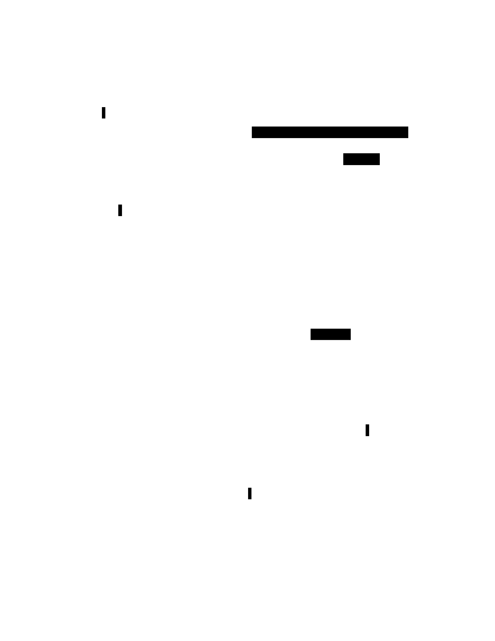
5. P(H) = P ′(H). This should be true because seeing the flip provided no

information about whether the coin landed heads. (Note that this would be

false if you had meaningful information about p, in particular a a sharp

credence of anything other than

Put these together and we derive ,

contradicting claim 1. White’s conclusion is to deny that 1 is rationally

permissible — rather, we should begin with a sharp credence of via the

Principle of Indifference. What should the proponent of unsharp credences do

instead? Joyce [2010] moves instead to deny claim 5 and set P ′(H) to equal P(q).

Paradoxically, this causes an dilation of your credence in P(H) — your P(H) was

precisely but your P ′(H) has become unsharp or interval-valued. Seeing the

coin land has apparently reduced your knowledge!

My response to the coin puzzle is to affirm Joyce’s view and accept dilation,

combined with the rule (maximin expected utility) given by Ga¨rdenfors and

Sahlin [1982] for betting on unsharp credences. According to this view, the

correct action for an unsharp agent with credence interval P(q) = [0,1] is as

follows: before seeing the outcome of the flip, it is permissible to buy and sell

bets on H for 0.5, to buy bets on p for prices ≤ 0, and to sell bets on p for prices ≥

1. After the outcome of the flip has been revealed, your betting behavior for H

should dilate to match your behavior for p. But, on my view, it is only your

credences that dilate — your frequency judgment that is exactly the

fragment of your knowledge that is not destroyed by seeing the p-side of the

coin come up.

This is the “conservative betting” behavior that White discusses and rejects.

His argument against it uses a scenario of long-run betting on repeated

instances of the coin puzzle, with a series of coin flips headsi and a different

unknown proposition pi each time:

On each toss you are offered a bet at 1:2 [i.e., for a price of ] on

headsi once you see the coin land pi or ¬pi. Since your credence in

headsi is mushy at this point you turn down all such bets. Meanwhile

Sarah is looking on but makes a point of covering her eyes when the

coin is tossed. Since she doesn’t learn whether the coin landed pi her

credence in headsi remains sharply and so takes every bet [....] Sure

enough, she makes a killing.

This hinges on an ambiguity in how exactly the bets are being offered. If you

know for certain that the bets will be offered, i.e., if you have a commitment from

your bookmaker to sell the bets, then that is equivalent to the bets being offered

before the coin is tossed, and you are justified in buying them. But if your

bookmaker can choose whether or not to offer the bet each time, you would be

very ill-advised to buy them, since he can then offer them exactly in the cases

when he knows that ¬pi, and you will lose your $ every time! This is exactly the

situation that unsharp credences are intended to prevent: if you suspend

judgment and refuse to bet, you can’t be taken advantage of. And once the pi or

¬pi side of the coin has been revealed, you can be taken advantage of by someone

who knows the truth about pi, so you should stop buying and selling bets. But

what has changed is your betting behavior about H, not your knowledge about

H. Your knowledge is exactly your frequency judgment and it remains intact.

The coin puzzle is a powerful illustration of the following fact: knowledge

about probability, the intuitive idea of “credence”, and betting behavior can all

come apart. Thus, it is only paradoxical under interpretations of probability in

which they are synonymous, or in which their synonymity is taken to be an ideal.

My hope is that the three-tiered interpretation can distinguish them in a natural

way, and in a way that affirms the core intuitions of frequentism.

3.12 Acknowledgements

I am grateful to Sherri Roush, Thomas Icard, Lara Buchak, Alan Ha´jek, Justin

Vlasits, Roy Frostig, Jacob Steinhardt, Andre Kornell, Paul Christiano, and Jason

Auerbach for helpful discussions.

Appendix: towards a convergence theorem for

frequency judgments

My objective here is to conjecture a convergence theorem that, if true, would

offer a distinctive kind of philosophical evidence for the claim given in section

3.5: that given a sequence of repeated trials of an event, two agents can

eventually come to agreement about their frequency judgment for that event,

even if they have different Bayesian priors, or if one is a frequentist and the

other a Bayesian.

Why is this conjecture distinctive? It is not a hypothesis of the theorem that

there exists a true limiting relative frequency for an event E, nor that Nature can

promise us a stream of likelihoods that will differentiate E from its negation.

Rather, it is a methodological assumption of the participants in the debate that

repeated trials of E can be modeled as i.i.d. draws from a single distribution. The

conjecture then says that they can agree in advance to perform some number of

trials, and as long as they continue to accept this assumption after the trials have

been performed, they will come to agreement in their fractional-valued

frequency judgments for E. (There is an interesting question about what

happens when the outcomes of trials undermine this assumption — for

example, if they exhibit large blocks of

E’s followed by large blocks of E’s — but that is outside the scope of the result.)

Intuitively, any statistical method based on likelihoods should exhibit this

convergence property. However, different formalizations run into different

formal difficulties. For example, consider two agents with distinct frequency

judgments a < b for E. Intuitively, these two judgments can be differentiated by

likelihood — if the observed relative frequency of E comes out closer to a than to

b, the likelihood of this observation is higher given the hypothesis that a is the

correct relative frequency, so the evidence supports a. But in fact, there exists p

with a < p < b such if the true frequency of E is p, the hypotheses P(E) = a and

P(E) = b will be indistinguishable by likelihood ratio testing — a and b will be

equally bad estimates of the true value p. Therefore, we cannot formulate the

theorem in terms of agreement for point estimates.

A natural alternative is to consider interval estimates — we want to show

that the frequentist and Bayesian interval estimates will converge to each other,

and moreover will shrink so as to falsify either one or both of the agents’

original frequency judgments.

Conjecture 1. Fix an event E, an initial point estimate pf of P(E), and a Bayesian

prior (possibly satisfying some additional conditions) over possible values of Pτ(E)

with mean E[τ] = pb. Fix a confidence level . Then there exists n such that after nγ

i.i.d. trials of E, the frequentist binomial -confidence interval γ[fl,fh] for P(E) and

the -credible interval γ[bl,bh] for P(E) given by Bayes-Laplace estimation with asτ

the prior will satisfy the following properties:

1. (Agreement.) [fl,fh] ∩ [bl,bh] =  ∅.

2. (Falsification.) At most one of pf and pb is in [fl,fh] [∪bl,bh].

Chapter 4

Computational complexity theory

and the normativity of rationality

Abstract

Interpreted literally, Humean decision theories entail a variety of rational

obligations related to consistency — not only to be consistent oneself, but to

distinguish consistency from inconsistency. Given fairly modest hypotheses from

computational complexity theory (specifically, the existence of one-way

functions), I derive stark limitations on the possibility of meeting these

obligations. In particular, a physically realizable agent can generate instances of

decision problems, together with their solutions, such that no physically

realizable adversary can improve on random guessing in solving them. I argue

that these results fatally problematize the concept of rational obligation, and

discuss the remaining possibilities for a computationally relativized theory of

rationality.

4.1 Introduction

The argument I propose to make is fairly simple. On widely accepted Humean

decisiontheoretic accounts of individual rationality, such as the Savage axioms,

an agent may be in a position such that they are rationally obligated to choose a

specific action in response. In other words, the correct choice of action is

logically determined by the axioms of rationality, which are putatively

normative; an agent who chooses incorrectly is violating a norm of rationality.

Yet under our best available mathematical and physical accounts of computation

— specifically, the so-called extended Church-Turing thesis — it will not, in

general, be possible for agents existing in our physical universe to make these

optimal choices. For this would require the agent to be able to solve problems

that are, according to those models of computation, intractable. But “ought”

must imply “can”; therefore, the accounts of rationality cannot be normative in

the way they claim.

This is, on its face, a straightforward argument — but it also appears

vulnerable to straightforward objections. For Bayesians have long been aware of

the problems that computational concerns pose for theories of ideal rationality.

There is an extensive literature on them (under the headings of “the problem of

old evidence” and “the problem of logical omniscience”) and they are not

generally considered fatal to the project of characterizing ideal rationality in

Bayesian terms. How, then, does my proposed critique differ from others that

have been advanced?

In brief, I think the computational critique can be sharpened, perhaps

paradoxically, by considering easier computational problems — problems that

are computable, in the sense of computability theory, but not tractable, in the

sense of computational complexity theory. This approach yields three principal

benefits. First, it undermines a metaphor that is persuasive in the computability

setting — the metaphor of incrementally approaching ideal rationality. Second,

it shows clearly how computational issues are not separable from decision-

theoretic formalisms, but emerge from them naturally: we will see how, under

popular decision-theoretic frameworks, intractability arises immediately in a

class of simple betting games. Finally, an unproven but widely believed

asymmetry in the laws of computation gives us instrumental reasons to take the

problem seriously. Unlike the problems that inspired the classical literature on

logical omniscience, we have a clear picture of how an adversary — not an

oracle or Newcomblike demon with unbounded computational power, but

limited in the same ways as the agent — can easily generate problem instances

that the Humean agent cannot solve.

Making this argument equires borrowing heavy machinery from

computational complexity theory. (The machinery is so powerful, in fact, that

the main results here follow readily from well-known theorems: the Cook-Levin

and Goldreich-Levin theorems.) These techniques have not yet become

commonplace in analytic philosophy in the way that logical and probabilistic

methods have become the basic toolkit for formal epistemologists. So part of

what I am arguing here — following the suggestion of Aaronson [2011] — is

that they deserve to be. Computational complexity theory can inform the

practice of epistemology because it provides a rigorous way of thinking about

thinking — specifically, thinking about the cost of thinking — that transcends

any particulars of human cognition or the technological augmentation thereof.

4.2 A class of decision problems

The following scenario is adapted from Elga [2010]. Fix a propositional atom A:

this proposition may be true or false, and you may have arbitrary knowledge

concerning its truth value (perhaps you know A, or you know ¬A, or you have a

Bayesian subjective probability estimate , or you have some other

kind of knowledge about it, or you know nothing at all). You are offered two bets

concerning A, B1 and B2 — you may take either, none, or both. B1 costs $1 and

pays $3 if A is true, and B2 costs $1 and pays $3 if A is false. Elga argues that on

any reasonable theory of rational obligations (barring a few pathologies, such as

being indifferent to money) it is an obligation of rationality that you must accept

at least one of the two bets. This is because accepting no bets yields $0 and is

therefore dominated by accepting both bets, which yields a certain $1, no matter

the truth value of A. You might have reason to accept exactly one bet — for

example, you might know that ¬A, and therefore accept exactly B2 — but

accepting no bets is irrational.

This argument is extremely persuasive and I think it sets out a clear baseline:

if there are such things as rational obligations, this is one. The question I am

interested in is, where then do these obligations end? Let us now introduce an

extended class of Elga-like problems. Consider a setting in which there are n

total propositional atoms, p1,p2 ...pn. We now consider a “book” consisting of m

bets; each bet Bi costs $1 and pays $(m + 1) if a formula qi1 ∧qi2 ∧qi3 is true,

where each qij is a literal, i.e. either a propositional atom or its negation. For

example, B4 might pay out on p3 ¬∧p6 ¬∧p9. As before, the agent may select any

subset of the bets, including the empty set.

Now, on a typical theory of normative rationality, many different preferences

over these bets will be permissible, depending on the subjective attitudes of the

agent. For example, it is compatible with the Savage axioms for an agent to have

linear utility in money and to adopt the uninformative prior over the pi, that is,

to consider them mutually independent, each with probability . In this

case, the agent’s Savage-rational betting behavior is very simple: each bet

independently contributes an expected utility of ( , and

in the case where m > 6 it is rationally obligatory to accept every bet (indeed, for

large m they are quite a good deal).

The problem that concerns me is this: according to some theories of

rationality, an agent may have attitudes on which it is not rationally permissible

to evaluate the bets independently — rather, the agent may have a rational

obligation to consider their interrelationship. For the bets as constructed have

the following property: they yield a sure profit exactly in the case where the

formula:

F = _ (qi1 ∧qi2 ∧qi3) (4.1)

1≤i≤m

is a propositional validity (i.e., is true under every possible truth assignment to

the atoms pi). To see this, suppose first that the formula is false: then every

clause of it is false and every bet loses, so accepting any nonempty subset of the

bets yields a loss. Conversely, if the formula is true, then at least one clause of it

is true; when all the bets are bought together, the bet corresponding to the true

clause yields proceeds of m+1, relative to an outlay of m to buy all the bets.

Now, on many Humean accounts of rationality, an agent may be rationally

obligated to buy a nonempty set of bets if and only if they yield a sure profit. The

agent’s reasons may be pragmatic or epistemic; an example of each will make

the situation clear. Consider first a Savage-rational agent (one guided by the

norm of expected utility maximization, or EUM) with the uninformative prior

over the Pi, but the following utility function in money:

(

xif x ≥ 0

u(x) = (4.2)

x − m3 · 2nif x < 0

This utility function is free of obvious pathologies (for example, it is

monotonic upwards in money). But it is constructed such that if F is not a

propositional validity, the expected utility of any nonempty subset of bets is

negative. To see this, note that if F is not a propositional validity, the probability

that it is false is at least , i.e. the probability mass assigned to a single non-

satisfying truth valuation by the agent’s uninformative prior. Meanwhile, the

maximum yield from any subset of bets is at most m(m + 1), which is smaller

than m for sufficiently large m. So the possibility of losing even $1 “swamps,” in

expectation, the positive utility from even the largest possible profit. So if F is

not a validity, the agent has a rational obligation not to buy any bets, but if F is a

validity, the agent has an obligation to buy some nonempty subset of bets.3

Alternately, consider the “maximin expected utility” (MMEU) framework of

Ga¨rdenfors and Sahlin [1982]. Eliding details which are not relevant to our case,

MMEU is a Humean framework that relaxes Bayesian constraints on knowledge

representation to allow “unsharp” credences, for example, interval-valued

credences P(A) = [l,h] that are interpreted as “my credence in A is somewhere

between l and h.” Then, each action can be valued according to its minimal

expected utility, i.e. the minimum value of its expected utility across all sharp

credences possible under the unsharp credence constraints. For example, if P(A)

= [.4,.7] and the agent has linear utility in money, a bet that pays $1 on A has an

indifference price of $0.4, and a bet that pays $1 on ¬A has an indifference price

of $0.3.

Consider an agent who adheres to MMEU and has linear utility in money, but

whose interval-valued credence in each pi is [0,1]. If F is a propositional validity,

then there is a rational obligation to accept a nonempty subset of bets (the full

package of bets yields a profit of at least $1, so 1 is a lower bound on the

minimum expected utility of the whole package; buying no bets has a minimum

expected utility of 0 and is therefore disallowed). But if F is not a propositional

validity, then there is at least one non-satisfying assignment S, and the space of

possible credences includes one that assigns probability 1 to that assignment.

Therefore, for any nonempty package of bets, its minimum expected utility is at

most its expected utility under S, which is −m. This entails a rational obligation

to accept no bets.

One may object to the use of extremal credences here. “Cromwell’s Rule”, so-

called, states that agents should never assign (sharp, real-valued) credences of 0

to any event that is logically possible, because such credences cannot be updated

by conditionalization. An extension of the rule to interval-valued credences

might rule out credences of the form [0,1].

But the appeal to such credences is inessential to the argument, because interval

endpoints sufficiently close to 0 and 1 will also exhibit the problem. It suffices to

choose ϵsatisfying

(4.3)

and then to replace [0,1] with [ ,ϵ1 − ϵ]; see Section 4.9 for a proof.

The potential obligation of rationality we have identified — the ability to

recognize propositional validities — appears modest. But according to our best

understanding of physical computation, it is too great to bear. To understand

why, it is necessary to introduce some notions from computational complexity

theory.

4.3 Computational complexity theory

Unlike recursion (or “computability”) theory, in which the main objects of study

are problems that cannot be solved by any computer, computational complexity

theory studies the relative hardnesses of problems that computers can solve.

Speaking very loosely, the problems we are ordinarily accustomed to solving

with computers (arithmetical operations, sorting, shortest paths in maps, etc.),

are in the complexity class P, meaning that they can be solved within a time that

is polynomial in the size of the input.

There is a natural class of prima facie harder problems, known as NP.

Intuitively, problems in NP have the following form: they can be computed by an

algorithm that “guesses” a solution from an exponential search space, then

verifies it in polynomial time. The canonical problem of this type is SAT, or

Boolean satisfiability: the question of whether a formula of propositional logic is

true under some assignment of truth values to the atoms. Checking whether a

particular assignment satisfies the formula is easy (i.e., polynomial-time), but

given n atoms, there are 2n possible assignments overall — thus, the brute-force

solution to SAT requires time at least exponential in the size of the input. P is

clearly contained in NP. Although it is strongly suspected that in fact P = NP, this 

has not been proven; it is considered one of the major unsolved problems in

contemporary mathematics.

The “hardest” problems in NP are called NP-complete. Their defining

characteristic is that every problem in NP is reducible to them, so if any of them

were discovered to be in P, it would imply P = NP. (Specifically, for any NP-

complete problem Q, there is a polynomial-time many-one reduction, or Karp

reduction, from any problem in NP to Q.) Problems outside NP may be NP-hard,

intuitively, at least as hard as NP-complete problems. (Formally, Q is NP-hard if

there is a polynomial-time Turing reduction, or Cook reduction, from any

problem in NP to Q.)

SAT is NP-complete. It has subproblems called k-SAT that are also NP-

complete:

Theorem 3 (Cook-Levin, Karp). A literal is a propositional formula of the form a

or ¬a, i.e., a positive or negated atom. Let a k-ary disjunction be a disjunction of k

literals; likewise for k-ary conjunctions. For k ≥ 3, the problem k-SAT of

determining the satisfiability of conjunctions of k-ary disjunctions is NP-complete.

I will idiosyncratically refer to the problem of deciding whether a

propositional formula is a tautology as VAL (for “validity”). The specific form of

VAL where the formulae are disjunctions of 3-ary conjunctions of literals (by

analogy with 3SAT) will be called 3VAL. VAL and 3VAL are unlikely to be in NP

(they naturally fall in the class co-NP instead), but since they are the

complement problems of SAT and 3SAT, they are as hard:

Proposition 1. VAL and 3VAL are NP-hard, and any lower bounds on the running

time of SAT and 3SAT (respectively) apply to them as well.

Proof. Assume a lower bound Ω(f(n)) for 3SAT, but an asymptotically faster

algorithm for 3VAL that is O(g(n)) (i.e. with g(n) = ω(f(n))). Take an instance of

3SAT of the form:

(a ∨b ¬∨c) (¬∧b ∨d ∨e)...

and compute its negation:

(¬a ¬∧b ∧c) (∨b ¬∧d ¬∧e)...

Apply the algorithm for 3VAL, then invert the answer (a formula is satisfiable iff

its negation is not a validity). The transformation is polynomial-time, so this is a

Cook reduction from 3SAT to 3VAL. Moreover, the transformed formula has the

same number of variables and clauses as the original, and we invoked the

algorithm exactly once, so we have an O(g(n)) algorithm for 3SAT, contradicting

the lower bound.

The proof for SAT and VAL is similar. □

What, then, is known about time lower bounds on SAT and 3SAT? Here the

exponential time hypothesis of Impagliazzo and Paturi [2001] is relevant. It has

various forms, but in general it says that the hardest NP-complete problems

cannot be solved in subexponential√

time, i.e., 2√o(n). For example, O(2 n) is considered subexponential under this

definition, but

O(( 2)n) = O(20.n) 2∈O(n) is not, even though both are asymptotically faster than

O(2n). As with P = NP, the ETH is unproven but widely believed. 

Conjecture 2 (Exponential time hypothesis). For each k, let sk be the infimum

(greatest lower bound) of the set of reals { δ| k-SAT is solvable in O(2 nδ)}. For k ≥ 3,

sk > 0.

We have known upper bounds on s3, the best due to Moser and Scheder

[2010]:

Theorem 4. 3-SAT is solvable in , for arbitrarily small ϵ

> 0.

Consequently, s3 ≤ 0.416.

So there are solutions to 3-SAT that asymptotically outperform brute force,

despite still being exponential.5 But in the general case, we have a (slightly

stronger again) conjecture by the same authors:

Conjecture 3 (Strong ETH). limk→∞ sk = 1.

The Strong ETH says that for larger and larger values of k, the optimal

solution of k-SAT regresses progressively to the brute-force O(2n) solution that

tests all possible assignments. We can now restate in complexity-theoretic

language the results proven in section 4.2:

Definition 3. Let DUTCHBOOK be the following decision problem. Given a book of

propositional bets over n atoms, does there exist a package of bets that yield a

profit under all 2n outcomes?

I will refer to such books as “Dutch books”, and to bets lacking this property

as “coherent books,” because they correspond respectively to incoherent and

coherent probability distributions.

Proposition 2. 3VAL is Karp-reducible to DUTCHBOOK, and 3SAT is Cook-

reducible to DUTCHBOOK; therefore DUTCHBOOK is NP-hard.

Proof. A 3VAL instance has the form

qi1 ∧

qi2 ∧qi3 1≤i≤m

where the qij are literals. Consider the betting book with bets B1,B2 ...Bm, such that

each bet Bi costs $1 and pays $(m + 1) if qi1 ∧qi2 ∧qi3 is true. As discussed in

Section 4.2, this book is Dutch if and only if the original formula is a validity; this

is a Karp reduction of 3VAL to DUTCHBOOK. For the Cook reduction of 3SAT to

DUTCHBOOK, one combines this with the Cook reduction of 3SAT to 3VAL given

in proposition 1: negate the 3SAT formula, convert the resulting 3VAL formula to

a betting book, apply the algorithm for DUTCHBOOK, and negate the answer. □

This result has long been known in the literature; Paris [1994] describes it as

“folklore.”Hardness results for various natural problems in the Savage

framework follow immediately.

Corollary 3. Given an oracle for an agent’s preferences over acts within the Savage

framework, determining whether those preferences are consistent with the Savage

axioms (i.e. whether there exist a subjective probability distribution and utility

function that represent them) is NP-hard.

Proof. Take an arbitrary 3SAT formula, negate it, and convert it to a betting

book via the technique in proposition 2. Consider an agent who strictly prefers

more money to less, and when faced with this book, strictly prefers the empty

package of bets to the package of all the bets. This agent can be represented by a

subjective probability distribution and utility function if and only if the original

3SAT formula is satisfiable. (If the formula is unsatisfiable, then the book is

Dutch and any expected utility maximizer with a strictly increasing utility

function must strictly prefer the package of all bets. Conversely, if the formula is

satisfiable, then there exist distributions and utility functions that model the

agent, e.g. a linear utility function combined with a distribution that assigns

probability 1 to the satisfying assignment.) This yields a Karp reduction of 3SAT

to the decision problem of whether such a distribution and utility function exist.

□

One might ask instead: if we are guaranteed that the preferences are

consistent, does the problem of extracting their Savage representation become

tractable? It does not:

Proposition 3. Assume that RP = NP  . Then there is no polynomial-time algorithm

that takes as input a Savage-consistent set of preferences, and outputs a

(polynomial-time computable representation of a) utility function and (P-

samplable representation of a) subjective probability distribution that represents

those preferences.

I will sketch the argument here; a rigorous proof is deferred to appendix

4.11, since it involves introducing some technical definitions that are not

otherwise relevant. First, we observe that given a 3SAT formula that is

guaranteed to be satisfiable, the function problem of computing a satisfying

assignment is still intractable; if it were tractable, one could feed in an arbitrary

formula and verify whether the output is in fact a satisfying valuation, thereby

deciding 3SAT in the general case. Now, given a satisfiable 3SAT formula, we

construct preferences for the agent that constrain the subjective probability

distribution to assign P(qi1 ∧qi2 ∧qi3) = 0 for each clause of its negation. It

follows from this that the agent must assign probability 1 to assignments that

satisfy the formula. Since the agent “knows” at least one satisfying assignment,

we can make him “tell” us; we will be able to recover a satisfying assignment,

even given relatively weak assumptions about how the probability distribution

is represented.

Proposition 4. Given an arbitrary betting book, subjective probability

distribution, and utility function as inputs, computing the action that maximizes

subjective expected utility is NP-hard.

Proof. Take an arbitrary 3SAT formula, negate it, and convert it to a betting

book as above. Combine it with the uninformative prior over the propositional

atoms, and the utility function from equation (4.2). The package of bets that

maximizes expected utility is empty if and only if the original formula was

satisfiable. This yields a Karp reduction of 3SAT to the function problem of

computing the expected-utility-maximizing action. □

Proposition 5. Given an arbitrary betting book and unsharp subjective

probability distribution as inputs, and assuming linear utility in money, computing

the MMEU-optimal action is NP-hard.

Proof. Take an arbitrary 3SAT formula, negate it, and convert it to a betting

book as above. Combine it with the unsharp probability distribution assigning

[0,1] to every atom, or alternately the unsharp probability distribution

described in Section 4.9. The MMEUoptimal package of bets is empty if and only

if the original formula was satisfiable. This yields a Karp reduction of 3SAT to

the function problem of computing the MMEU-optimal action. □

4.4 Average-case complexity

Thus far, all the hypotheses we have considered concern worst-case complexity,

i.e., they assert that for any algorithm, there exist cases which it cannot solve

efficiently. However, they leave open various possibilities in the realm of

average-case complexity that would suggest a more hopeful outlook. Impagliazzo

[1995] gives evocative names to five epistemically possible worlds (i.e.

mathematical possibilities for complexity theory that are not yet ruled out by

unconditional results), each with different consequences for our class of

problems. The first possibility (which he calls “Algorithmica”) is that P equals NP

— as discussed, this would allow efficient recognition of Dutch books, but is a

highly implausible outcome. But there are two other possible worlds in which

expected utility maximization might be a tenable norm:

1. An efficient algorithm could exist to solve 3VAL and therefore

DUTCHBOOK; eventhough it would fail on some inputs, those inputs would

be vanishingly rare and moreover difficult to find. One could therefore

confidently expect the algorithm to work on all betting books encountered

in practice. (Impagliazzo calls this possible world “Heuristica”.)

2. An efficient algorithm could exist to solve 3VAL and DUTCHBOOK; it would

fail ona significant number of inputs, but those problem instances would

be hard to solve for any algorithm, including one with control over the

inputs. (Impagliazzo calls this possible world “Pessiland”; it is the “worst”

world for applied computer science because even though it lacks efficient

algorithms for arbitrary NP problems, it also lacks secure cryptography.)

However, an additional widely-believed hypothesis excludes both of these

possibilities. Under this hypothesis, it will be possible to generate new betting

book instances, together with short proofs either of their coherence or their

Dutchness, that are too hard for any efficient algorithm to solve. Specifically, in

Impagliazzo’s final two worlds, “Minicrypt” and “Cryptomania”, one-way

functions exist; the hypothesis that an injective one-way function exists will be

sufficient to carry out this construction.

Unlike the previous hypotheses, the definition of a one-way function is

necessarily probabilistic. We first introduce the notion of a negligible function: a

function ϵ(n) is negligible if for all c, it is eventually less than . (For example,

and are negligible, but is not.) Now, a one-way function is a function that

is easy to compute, but hard to invert; it “scrambles” its input in some way such

that it is hard to recover any preimage of a function output, in a robust

probabilistic sense.

Definition 4. A polynomial-time computable function f is one-way if for every

probabilistic polynomial-time algorithm A, there is a negligible function suchϵ

that for every n,

In other words, for any A that tries to reverse f, when we sample over all

possible inputs x and executions of A, A is unlikely to find a preimage of f(x).

One-way functions have a variety of interesting implications; for example, a

deep theorem of H˚astad et al. [1999] shows that they imply the existence of

pseudorandom generators indistinguishable (by polynomial-time adversaries)

from true randomness. But for our purposes, a simpler construction will suffice.

According to a result of Goldreich and Levin [1989], without loss of generality,

we may assume that a one-way function has a hard-core predicate:

Definition 5. Let f be a one-way function. A hard-core predicate h of f is a function

mapping inputs of f (bitstrings of length n) to single-bit outputs (elements of {0,1})

such that for any probabilistic polynomial-time algorithm A, there is a negligible

function such that for every n,ϵ

That is to say, for any A that tries to predict the value of h(x) given f(x), when

we sample over all possible inputs x and executions of A, it cannot significantly

improve on guessing the value at random.

To motivate this additional notion, note that the definition of a one-way

function leaves open the possibility that any individual bit of the input might be

predictable. However, since the input cannot be predicted in totality, it seems

intuitive that a “mixture” of all the bits together should also be unpredictable.

Given a one-way function f, the Goldreich-Levin theorem provides an effective

construction of a modified function f′ and a “mixing” predicate h that is hard-core

for f′.

Now, let us strengthen our hypothesis slightly and assume the existence of f

that is both one-way in the above sense and injective (i.e. if x and y are inputs of

length n then x = y implies f(x) =  f(y)). (Within the hierarchy of cryptographic

hardness assumptions, this is considered only slightly stronger; see Section 4.10

for details.) We observe that the GoldreichLevin construction, when applied to

an injective function, preserves its injectiveness, so, without loss of generality,

we may assume that f is one-way, injective, and has a hard-core predicate. Let us

moreover assume that an agent can have access to an unpredictable source of

random bits: paradigmatically, this is the ability to “flip coins” or access some

other source of apparent physical indeterminism. It is not necessary to assume

that physical chance exists in a metaphysical sense, only that the agent’s real-

world adversaries cannot predict or model the process better than as i.i.d. draws

from the uniform distribution over {0,1}.

Proposition 6. Suppose an injective one-way function f exists. Then it is possible to

generate cryptographically indistinguishable Dutch and coherent books in

polynomial time. Specifically, it is possible for a polynomial-time agent G with an

unpredictable source of randomness to generate both Dutch and coherent betting

books over n propositions, such that G knows whether the book is Dutch or not, but

no probabilistic polynomial-time adversary A can determine this with probability

greater than , where is a negligible function.ϵ

Proof. As discussed, we may assume that f has a hard-core predicate h. The

agent G uses his source of randomness to generate an unpredictable input string

x of length n. Then, G generates an additional bit of randomness q to decide

whether the book will be coherent or Dutch. If the book is to be coherent, G

reveals f(x) and h(x) and sets the following decision problem: does y exist such

that f(y) = f(x) and h(y) = h(x)? If it is to be Dutch, the agent does the same but

after inverting the value of h(x), i.e.: does y exist such that f(y) = f(x) and h(y) = 1

− h(x)?

These problems are in NP because both f and h are polynomial time, so a

guessed value of y can be verified in polynomial time. Note however that in the

first case, the problem has a solution (x) and in the second case it has no

solution (since f is injective, there can be no second preimage y such that h(y) =

1 − h(x)). Consequently, G can apply appropriate reductions to transform this

problem into a SAT instance. The SAT instance can then be transformed into a

3SAT instance, then into a 3VAL instance and finally into a betting book via the

reduction given in Proposition 2. If the original problem had a solution, the book

will be coherent; if it did not, the book will be Dutch.

Suppose a polynomial-time algorithm A could achieve more than negligible

advantage over in determining whether a resulting book is Dutch or not. Given

a random output f(x), one could then consider the decision problem “does y exist

such that f(y) = f(x) and h(y) = 0?”, apply the relevant reductions to produce a

betting book, then apply A. If A indicates that the book is non-Dutch, then output

0, otherwise 1. This algorithm achieves the same non-negligible advantage in

predicting h(x) from f(x), contradicting the assumption that h is a hard-core

predicate. □

Two things should be noted about this construction. One is that even though

we used a random bit to decide whether the book was to be Dutch or coherent,

this assumption can be relaxed: as long as the input x of the one-way function is

chosen at random, this decision can be made arbitrarily. The problem is that an

adversary might then be able to detect and exploit a higher-level pattern in the

sequence of which books are Dutch — for example, if G was such that every third

book was Dutch and the others coherent, an adversary A could be constructed to

predict this perfectly without even examining the books. (Hence the necessity of

the random bit to prove our desired probabilistic hardness claim.) Yet any such

advantage must depend on assumptions about the agent G, rather than on

deductions from the betting book itself, in the following sense:

Corollary 4. Suppose an injective one-way function exists. Then there is no

probabilistic polynomial-time algorithm A such that for any agent G generating

betting books over n propositions, A can distinguish G’s coherent and Dutch books

with probability greater than , where is a negligible function.ϵ

Proof. Take G to be the agent constructed in the previous proof (using a

random bit for each book); this then follows immediately. (Note moreover that a

probability of exactly can be achieved through random guessing, so this is a

tight upper and lower bound.) □

In contrast, G himself knows a short, polynomial-time verifiable proof for the

status of each book, whether it is Dutch or coherent: he can simply reveal the

hidden value of x. Then any polynomial-time observer can compute h(x),

compare it to the revealed value, and conclude whether a satisfying assignment

exists or not.

Here is a brief illustration of the level of control G enjoys over these

problems. Suppose G uses this procedure to generate a coherent book; through

the construction, he also has access to the falsifying truth assignment, meaning

the propositional valuation such that all the bets lose. Suppose further that G has

access to a stock of obscure true statements that can be negated without

significantly altering their syntax, for example “Childeric I of France reigned

before Chilperic I of France” or “the closing value of the Dow Jones index on

January 3rd, 1991 had an odd number of cents”. He can then assign the

questions or their negations (which will not be syntactically distinguishable) as

the definitions of the propositions p1,p2 ...pn so that their truth values coincide

with the falsifying truth assignment. Now, consider an agent A who is presented

with this book, but has no specific information about the true-or-false questions.

To A, this book appears indistinguishable from a Dutch book: out of the 2n

possible truth assignments, only 1 is falsifying, and computing that assignment

from the book is intractable because f is a one-way function. But if A accepts any

of these bets, she loses. This is not to say that this kind of “cardsharking” is

necessarily a significant concern for decision theory — I am sympathetic to the

argument of Al-Najjar and Weinstein [2009] that adversarial problems like these

should be studied via game theory instead — but it demonstrates the extent to

which these problems confound naive attempts at probabilistic analysis.

Let us briefly discuss the implications of these results for physical

computation. The Church-Turing thesis states that all physically realizable

computation can be modeled by the Turing machine, implying any problem that

is undecidable in the Turing machine model cannot be solved in general by

physically realizable computers. A variety of proposals have been advanced for a

complexity-theoretic analogue of this hypothesis, typically under the name

“extended Church-Turing thesis”. Originally it was hypothesized that efficient

realworld computation was captured by the complexity class P, meaning that

problems outside of P cannot be solved by physically realizable computers

within realistic amounts of time. This conjecture has been complicated by the

apparent phenomenon of quantum supremacy, meaning that scalable quantum

computers will be able to solve some problems outside of P. At present, the

following conjectures are generally believed:

1. Physically realizable computation is captured by the complexity class BQP

(looselyspeaking, the problems that can be solved by quantum computers

in polynomial time). This class contains both P and BPP (the class of the

probabilistic polynomial-time adversaries we invoked in our definition of

one-way functions).

2. NP-hard problems are not in BQP [Aaronson, 2005]; therefore, physically

realizablecomputers cannot recognize sufficiently large Dutch books, or

maximize expected utility under the constraints described in Proposition

3. Although the definition of one-way functions we used above referred only

to classicaladversaries, there also exist classically computable one-way

functions secure against quantum adversaries. Consequently, Proposition 6

is still true even if we grant the adversary B the power of BQP, instead of

just BPP; we can generate Dutch and coherent books that cannot be

distinguished by any physically realizable agent in a realistic amount of

time.

4.5 The problem of logical omniscience

Epistemological abstraction

I will take recent work by Elga and Rayo [2022] as paradigmatic of current

proposals for resolving the problem of logical omniscience. The authors are

concerned with apparent violations of rationality that arise from human agents’

inabilities to access all logical implications of their knowledge. For example, an

agent may be aware that a simple contradiction A¬∧A is unsatisfiable and

should be assigned probability 0, but may assign nonzero probability to a more

complex sentence that is also a contradiction and therefore logically equivalent

to the first. Alternatively, an agent might believe the axioms of Peano arithmetic,

but also assign nonzero probability to the so-called P´olya conjecture (a

sentence of first-order arithmetic that is plausible, but disprovable from those

axioms). Their solution is to provide a plural model of epistemic states: an agent

is modeled by an access table containing multiple subjective probability

distributions. Each “row” of the access table corresponds to a “choice condition,”

an epistemic state in which some subset of the agent’s knowledge has been

made “salient” or immediately accessible — “at the forefront of [the agent’s]

mind.” The access table maps each choice condition to a probability distribution

over sentences that is coherent, but which does not respect all logical

implications among sentences — only among those sentences that have been

made salient. Rational decision-making is then governed by the “fragmented

choice rule”:

A subject in choice condition c should act as though to maximize

expected utility relative to Pc, where Pc is the probability function

associated with subject c in the subject’s access table.

I think this model is at least prima facie successful at dealing with the

paradigmatic cases that have long bedeviled Bayesian accounts of knowledge:

mathematical conjectures whose proofs are ultimately determined to follow

from old axioms, and scientific theories that are confirmed by “old evidence”

[Glymour, 2010], i.e. old empirical observations that are only understood as

confirmatory after new mathematical consequences are drawn out of the theory.

Elga and Rayo’s insight is that in such cases, the non-omniscient agent is faced

with an epistemic possibility that is not a logical possibility (e.g., that the axioms

are true but the theorem that follows from them is false). Through a possible-

world semantics that tracks epistemic possibility by abstracting away the true

logical relationships among sentences, they are able to construct a locally

coherent model in which notions like expected utility maximization (which is

conventionally defined over a coherent probability distribution) can be applied

directly.

But how does this model fare vis-a`-vis our problem cases? Consider the

expected-utilitymaximizing agent we constructed in Section 4.2. This agent

already possesses a coherent probability distribution over all the salient

sentences. Once the betting book is revealed, the conjunctions qi1∧qi2∧qi3 can all

plausibly be made salient to the agent — certainly to an agent augmented with a

physically realizable computer — and they all have probability . (Here it is

important that the successive reductions we applied to construct our

indistinguishable books — from the one-way function to a SAT instance to a 3-

SAT instance to a betting book — all increased the size of the problem instance

only polynomially. The problem is still small enough that the agent can fully

comprehend what is being asked.) The agent’s access table is apparently

trivialized, consisting of a single row. But we have shown that the agent, even

with computer augmentation, cannot apply the “fragmented choice rule,”

because it requires expected utility maximization — which is computationally

intractable for this distribution and utility function. This intractability cannot be

abstracted away via the access table formalism, because it emerges out of the

formalism itself — specifically out of its pragmatic or decision-theoretic

component. To achieve tractability, we need not only an epistemic relaxation, but

some relaxation of the pragmatic norm of expected utility maximization. But

what would such a relaxation look like?

Relaxation or strengthening?

First, a caution: some potential relaxations of the norm of Humean expected

utility maximization actually intensify the problem of computational

intractability. Consider, for example, Buchak’s [2013] risk-weighted expected

utility (REU). REU can be understood as a relaxation of the Savage framework

that imposes fewer constraints on the agent — in particular, one of the Savage

axioms of rationality (the “sure-thing principle”) is replaced with a weaker

alternative. But this weakening of constraints is also, paradoxically, a

strengthening. For REU contains the Savage framework as a special case: it adds

an additional Humean free parameter, the risk function, but an agent with a

linear risk function is rationally obligated to maximize expected utility. It follows

that REU can also entail a rational obligation to solve DUTCHBOOK.

In fact, if the risk function is allowed to vary, the ability to compute the REU

of an action can be applied to solve prima facie harder problems than expected

utility maximization. For example, with an oracle for REU, one could solve not

just SAT but #SAT (counting the number of satisfying assignments to a Boolean

formula) in polynomial time. Concerns of this form potentially apply to any

modification of EUM that makes the theory more expressive, in the sense of

being able to construe more agents as rational. As the logical characterization of

the optimal action becomes more complex in structure, the complexity of

computing it may increase as well. (Conversely, if we were to constrain the

Savage-rational agent further by requiring linear utility in money, the class of

intractable problems studied here would be excluded, and the approach of Elga

and Rayo [2022] would be prima facie adequate to save expected utility theory.

But such a constraint is persuasive at neither a normative nor a descriptive

level.)

Approximating ideal rationality

Let us consider relaxations of the norm of expected utility maximization that

preserve the concept of expected utility. There are two distinct paths that a

computationally limited agent can take on our class of problems. One is to buy

no bets, which achieves a guaranteed utility of 0: this is the only action that an

agent unable to solve DUTCHBOOK can prove to have nonnegative expected

utility. One may think of this option as relaxing the requirement of

maximization, while preserving the concept of expected utility. However, this

strategy can fail arbitrarily badly relative to the optimal action. For example, one

may multiply the utility function in (4.2) by an arbitrary factor c without

changing the relevant properties (buying the bets is still recommended if and

only if the book is Dutch). Then, in the case where the book is actually Dutch,

this strategy underperforms the optimal expected utility by at least c.

The other path is to buy some nonempty subset of the bets without the

assurance that the book is Dutch. I claim that any such strategy fails to take the

premises of Humean expected utility seriously — it relaxes the concept of

expected utility itself. If the utility function is truly a free parameter, determined

by the agent’s sovereign preferences and constrained only by basic

requirements of consistency, then it follows inexorably that even an vanishingly

small probability of an astronomically negative outcome can outweigh a near

certainty of modest gain.

But should we, in fact, take these premises seriously? I propose that

vanishingly small probabilities p are real — grounded in physical realities — in a

way that large utilities on the order of are not. We can readily instantiate

physical scenarios in which welldefined events have exponentially low

probabilities, for example, by flipping 10,000 coins and considering the

possibility that they all land heads. But how good or bad can things get for

agents in our physical world? It seems to me that plausible bounds on the

magnitude of a utility function can be derived from constraints like the number

of electrons in the universe. Following this suggestion leads to the conclusion

that our class of problems cannot, in fact, be “scaled” indefinitely: at some point,

the negative utility must be clamped so that it no longer outweighs the positive

utility, making it licit for the expected utility maximizer to buy the bets.

Is this enough to put these troublesome cases to rest, by denying that they

actually entail a rational obligation to solve intractable problems? It might be for

a non-Humean who is still a Bayesian, and who therefore affirms a rational

obligation to assign sharp credences. But in the end, it won’t do for me, because I

affirm the rational permissibility of unsharp credences and MMEU as a response

to non-probabilistic uncertainty (or “Knightian uncertainty”). As discussed in

Section 4.2, such an agent may also incur a prima facie rational obligation to

solve DUTCHBOOK. I will return to this question in Section 4.6. For now, I

contend only that it is unclear what it would mean to approximate ideal

rationality over our class of problems.

Approaching ideal rationality

There is another defense of a conventional concept of rational obligation:

principles like expected utility maximization might be normative despite the

impossibility of realizing them in practice, because they still function to guide

imperfect agents in the right direction. Here is Zynda [1996]:

Since there are no a priori constraints on what sorts of new methods,

shortcuts, or “heuristics” (including technological aids such as

“expert” machines) the human community may develop as we strive

to reach particular ideals that we set for ourselves, there is often no

reason to regard any part of a betterness ordering that is defined by

an unattainable ideal that we currently accept as completely

irrelevant to our personal obligations.

And here is Levi [1997]:

Still more importantly, the counsel of those who urge us to trim our

principles of rationality is the counsel of complacency. Of course, we

cannot be obliged to do at the moment what we cannot at that

moment do. We cannot be obliged to recognize all the logical

consequences of our full beliefs or even enough of the consequences

to solve some particular complicated problem. But we can be urged

(costs and time permitting) to seek therapy for our distress, to

devise prostheses to extend our computational capacities and

memories (such as computers, paper and pencil, handbooks of

tables, etc.) and to learn logic and mathematics so that we can to

some extent overcome our disabilities.

I highlight these passages not to definitively refute the underlying arguments,

but to suggest that they, like the epistemic theory discussed in Section 4.5, draw

their inspiration and their intuitive force from a different class of problems than

ours. These arguments resonate well with the problem of logical omniscience as

applied to mathematical and scientific truth. Even though we know that we

cannot currently resolve many open mathematical problems, there is no strong

justification for pessimism about our ultimate ability to resolve any particular

open problem; heuristically, we have numerous examples of longstanding open

[2011].

problems being successfully resolved. Metaphorically speaking, we may hope to

incrementally approach a state of perfect mathematical knowledge — as one

open problem falls, another conjecture may open up in its place, but we hope

that it too will fall. Moreover, there seems to be nothing pragmatically

embarrassing about not knowing the truth of (for example) the Riemann

hypothesis, since no one else in our world knows it either. A betting book that

assigns probability 0.99 to the Riemann hypothesis may well be Dutch, but the

issue is moot since there is no way to settle the bet.

But with our class of problems, we see that the “aids” and “prostheses” that

Zynda and Levi appeal to are of no avail. There may not be a priori constraints

on the prostheses we can build to solve decision problems, but the extended

Church-Turing thesis gives us a very strong putative empirical constraint: it is

physically impossible for an agent in our universe to solve these problems in

general. Rather than envisioning an endless ascent towards mathematical truth,

we may imagine an impenetrable barrier or firmament that separates us from

unreconstructed norms of decision-theoretic rationality like EUM. Moreover, due

to the asymmetrical nature of average-case complexity theory, hard problem

instances can be generated together with their solutions, and then the solutions

can be revealed and verified to settle the bets — all by a physically realizable

agent with the same computational capabilities as the would-be solver.

4.6 On the status of rational obligations

But Zynda has anticipated a key part of this criticism:

Finally, in those cases where we do have reason to believe that there

are limitations on how closely the ideal will ever be approximated,

our judgments of betterness [or] worseness with regard to the

feasible case are often in fact guided by the ideal: we define the ideal,

and then define what is “better” in terms of approximation to that

ideal, not the other way around. In such cases, there is a clear sense

in which the ideal is guiding our practice, even though it is itself

unattainable.

Let us step back from specific formalisms like expected utility maximization

and consider our problems in a pre-theoretic setting. Imagine an agent who has

reasons to accept only packages of bets that yield sure profit. It seems clear that

in Elga’s original singleproposition case, buying both bets is rationally preferable

to buying no bets, and moreover that buying no bets constitutes a breach of the

agent’s rational obligations. Furthermore, it seems to me that when one

considers increasingly complex cases (extending finally to the betting books

constructed in Proposition 6), the first judgment still holds: the agent able to

recognize whether such books are Dutch exhibits a superior facility of

rationality, and is meaningfully closer to ideal rationality. Here I am concurring

with Zynda that ideal conceptions of rationality retain some kind of normativity,

even in the face of complexity-theoretic impossibility results. But I think the

second judgment — that the agent unable to solve arbitrary books is in breach of

a rational obligation, or evincing a “failure of rationality” — is no longer

supported. Ought must imply can, and an agent in our physical universe cannot

solve these problems, nor make meaningful progress towards the ability to solve

them.

I hold, therefore, that the concept of “rational obligation” has been

problematized even if the concept of “ideal rationality” has not. What would it

take to save it? We would seemingly need a bright-line distinction somewhere

between the Elga case and the indistinguishable cases, separating tractable from

intractable problems. But on our best understanding of SAT and VAL, no such

distinction is possible; there is no “perfect” or “complete” solver that can solve

all the tractable instances. Rather, we have a messy patchwork of heuristics

[Biere et al., 2009] representing incremental progress, but which, as discussed,

cannot hope to approach the hardest problems in the space.

Moreover, if we try to make rigorous a view where rational obligations

coincide with tractability de facto, a troubling relativism emerges. We can

deliberately sabotage the construction in Proposition 6 by choosing a one-way

function that is believed to resist classical adversaries, but known to be

vulnerable to quantum adversaries, such as the RSA function [Goldwasser and

Bellare, 1996]. The resulting problem instances will be intractable to an agent

who lacks access to scalable quantum computation, but tractable to one with

such augmentation. The problem here is that unlike classical computing, which

“exists in nature” in the sense that humans can store and process classical

information by means of mundane objects such as pen and paper, scalable

quantum computing will require the creation and manipulation of highly

anomalous physical states, because achieving quantum advantage requires

protecting the qubits from quantum decoherence [DiVincenzo, 2000]. Scalable

quantum computing is not an extension or enhancement of classical computing

in the way that digital computers extended the possibilities already available via

“human computers” [Grier, 2013], but a phenomenon fundamentally different in

kind. This suggests that in order to save the concept of “rational obligation”, we

would have to relativize it: it would have to exist in (at least) two variants, one

for classical and one for quantum agents.

I think the natural conclusion is that the term “rational obligation” is both

vague and context-dependent — its meaning is entangled with the meaning of

“tractable,” which turns out to function much like the ordinary-language terms

“small” or “inexpensive” in resisting a precise definition. This is not to say that

the concept is of no philosophical use, but that we should be wary of its

susceptibility to paradox. For example, returning to axiomatic frameworks like

Savage’s, consider the agent who, faced with a hard Dutch book, buys no bets.

This agent is not maximizing expected utility and is therefore in breach of one of

the Savage axioms. But I have argued that this agent is not in breach of any

rational obligation — on this view, the Savage axioms do not unconditionally

create obligations of rationality.

4.7 On the status of ideal rationality

I have just argued that aspects of ideal rationality — in particular, the

recognition that some decisions really are better than others, regardless of

tractability concerns — are worth saving. But I think these results problematize

the way ideal rationality has been theorized.

The first problem is as identified in Section 4.5; if ideal rationality is

unachievable due to intractability, the natural move is to adopt a norm of

approximating ideal rationality instead. Zynda [1996] takes his defense of ideal

rationality to be contingent on such a project, because it is only through such a

“betterness ordering” of approximations that ideal rationality can still function

pragmatically to guide us. But in general we should expect multiple competing

(and mutually incomparable) concepts of approximation. As we saw with EUM,

one may preserve the concept of subjective expected utility while relaxing the

norm of maximization, or relax the concept of subjective expected utility. Which

answer is superior? The problem may well have a solution, but it is unlikely that

the theory itself will be able to provide it, since by definition we are operating in

a domain in which the theory has broken down.

Furthermore, if the ideal is unachievable, it is not clear why theoretical

acceptance of the ideal’s premises should mandate pragmatic acceptance of the

ideal’s methods. For example, one might accept the foundational principles of

Bayesian statistics at a theoretical level, but use frequentist methods in practice

given the impossibility of achieving the Bayesian ideal. There is consequently an

argumentative gap between typical attempts to prove the normativity of

Bayesianism (via the axiomatic method, Dutch Book arguments, etc.) and

advocacy for the use of Bayesian methods — pace Savage’s [1972] claim that his

axioms provide “the foundations of statistics.”

But the question that really interests me is this: why, as Diaconis [2003]

observes, is expected utility maximization so ineffective in practice at guiding

real-world decisions? To all the familiar practical issues with the framework —

individuation of outcomes [Bermu´dez, 2009], reconciliation of “small-world”

and “grand-world” models [Buchak, 2013], model uncertainty — one may add

another: even on toy problems that present none of these conceptual difficulties,

we find that applying the framework can be computationally infeasible. The

practical import of representation theorems is hollowed out by results like

Proposition 3, which show a computational barrier to actually extracting

subjective probabilities and utilities from preferences.

I am pessimistic about attempts to modify existing decision-theoretic

frameworks to take computation into account, because it seems to me that

computational omniscience is woven very deeply into their fabric. Take, for

example, Savage’s axiom of comparability, which states that a rational agent

normatively has a linear preference ordering over acts. Aside from concerns

about whether some acts might be genuinely incomparable, it seems to me that

the effect of this axiom is to reify the agent’s preferences as a “completed”

totality, making them simultaneously visible to the apparatus of the

representation theorem. In reality, however, some preferences might be

significantly harder to compute than others, or a computationally limited agent

might intentionally sacrifice the ability to compare acts that it would never have

to choose between in practice. I would suggest that for a computationally

bounded theory of rationality, an alternative program is to begin from the

bottom up: take systems that are known to be computationally efficient and then

interpret them retroactively as following (in full or in part) decision-theoretic

principles. In this way, a computational decision theory would be contiguous

with current work on AI “surveyability” or “explainability”.

4.8 Acknowledgments

Thanks to Julian Jonker, Sherri Roush, Wes Holliday, Roy Frostig, Justin Vlasits,

Adam Lesnikowski, Matt Jones, Umesh Vazirani, Justin Bledin, Scott Aaronson,

Adam Elga, Prasad Raghavendra, Daniel Fremont, and Avner Ash for helpful

discussions.

4.9 Appendix: A non-extremal unsharp distribution

for which MMEU is intractable

Consider the betting books defined in Section 4.2, where we have n

propositional atoms and m bets on formulae of the form qi1 ∧qi2 ∧qi3, each

costing $1 and paying $(m + 1) if the formula is true. We adopt a definition of

“unsharp probability distribution” as a convex family of ordinary (“sharp”)

probability distributions. We are seeking to construct an unsharp probability

distribution D over the underlying propositional atoms p1,p2 ...pn such that

1. D is non-extremal; for every sharp distribution P ∈D, P assigns nonzero

probability to every possible truth assignment.

2. MMEU (with linear utility in money) over D mandates buying a nonempty

subset of bets if and only if the formula (4.1) corresponding to the betting

book is a propositional validity. (This is the property necessary to support

the reduction in Proposition 5.)

As discussed in Section 4.2, if the formula is a propositional validity, then the

minimum expected utility (MEU) of the full package of bets is at least 1; since

the minimum expected utility from buying no bets is 0, this action is disallowed

by MMEU and the agent must buy some nonempty subset of bets. Assume then

that the formula has some falsifying assignment h. Fix ). Let D be the set

of all probability distributions P such that P assigns nonzero probability to every

truth assignment and furthermore P(pi) [∈,ϵ1 − ϵ] for all i. It is immediate from

the definition that D is convex.

Now, the MEU of the whole package of bets under D is bounded above by its

expected utility under any individual P ∈D. Consider P such that all the pi are

mutually independent and

i.e. given the constraints on P, it assigns the maximum possible probability (1 −

ϵ)n to the falsifying truth assignment h. If the expected utility of the full package

of bets under P is negative, then buying the whole package of bets is forbidden

by MMEU (since buying no bets has a MEU of 0).

The utility from the falsifying assignment is −m, while the utility from any

other assignment is at most m2, yielding the following upper bound on the

expected utility of the package under P:

E[X] ≤ (1 − ϵ)n · (−m) + (1 − (1 − ϵ)n)) · m2.

Let r = (1 − ϵ)n. We want E[X] < 0; it suffices to choose ϵsuch that

E[X] ≤ −rm + (1 − r)m2 < 0

Now, as m increases, this bound on ϵdecreases, so the bound produced for

the full package of m bets is also adequate for any nonempty proper subset of

bets. That is to say, when considering the MEU of a subset of m′ bets, where 0 < m

′ < m, we consider the book that consists only of those m′ bets and re-run this

argument. The resulting bound on c will be entailed by the bound above. □

4.10 Appendix: Some cryptographic context

I stated earlier that the assumption that an injective one-way function exists is

“slightly stronger” than the assumption that a one-way function exists. All claims

of this form must be regarded as metaphors, since in fact any such hypothesis is

either unconditionally true or unconditionally false in the “real world”. Claims

about relative strength should be understood as statements about known

implications between the hypotheses.

The construction in Proposition 6 aims to create a betting book with three

properties:

1. Given only the book as an input, it is intractable to determine whether the

book isDutch or coherent;

2. If the book is coherent, the generator can reveal a proof of its coherence;

3. If the book is Dutch, the generator can reveal a proof of its Dutchness.

If we carry out the construction using a one-way function that is not injective,

properties 1 and 2 are preserved, but 3 is not. The generator G can still reveal

the preimage x of f(x), and if h(x) coincides with the previously announced value

of the one-way predicate, A can verify that x yields a satisfying assignment. But if

h(x) contradicts the previously announced value, A cannot satisfy herself that

there does not exist some other x′ such that f(x) = f(x′), but h(x′) agrees with the

previously revealed value — which would make the book coherent after all.

It would therefore be useful for our purposes to be able to transform an

ordinary one-way function into an injective one, via a construction analogous to

the Goldreich-Levin theorem (which transforms an ordinary one-way function

into one with a hard-core predicate). Unfortunately, Rudich [1988] proved that

no such construction is possible in a “black-box” model, i.e. without relying on

specific properties of the candidate one-way function. This is discouraging but

not necessarily fatal for the project of constructing an injective one-way function

based on weaker hypotheses; see Rotem and Segev [2018] for recent work on

the question. Conversely, however, injective one-way functions are themselves a

weak hypothesis in the sense that it does not appear possible to use them to

construct trapdoor one-way functions or public-key cryptosystems (they would

not, by themselves, take us out of Impagliazzo’s “Minicrypt” and into

“Cryptomania”).

However, at a higher level of abstraction, these three properties correspond

to what is known in cryptography as a bit commitment scheme [Goldreich, 2001].

This is a protocol by which an agent G can fix a secret value b {0∈,1}, then reveal

a “commitment” c derived from b. It must be intractable for anyone to recover

the true value of b from c. However, it must also be possible for G to

subsequently reveal a secret value s that “opens” the commitment c. Specifically,

it must be tractable to compute the true value of b from both c and s together,

and moreover s must prove that G did not alter the value of b after c was

generated — in other words, once c is fixed, it must be intractable for G to

produce both a s that reveals b = 0 and a s′ that reveals b = 1.

Informally, then, constructions of indistinguishable betting books are

intertranslatable with bit commitment schemes. Proposition 6 corresponds to a

simple bit commitment scheme based on an injective one-way function f with

hard-core predicate h: given b, generate a random s, reveal f(s) and b⊕h(s) as the

commitment, then reveal s to open the commitment.But conversely, given a

typical bit commitment scheme, one can generate indistinguishable Dutch and

coherent books. Suppose without loss of generality that the true value of b is 0.

For a coherent book, at the final stage of the commitment scheme one sets the

decision problem, “does a secret value s exist that would open the commitment

and reveal 0?” For a Dutch book, one asks instead, “does s exist that would open

the commitment and reveal 1?” The appropriate reductions applied to the

(deterministic, polynomial-time) algorithm for opening the commitments will

yield SAT formulae and eventually betting books.

The good news, then, is that Naor [1991] gives a bit commitment scheme

based only on the assumption of a cryptographically secure pseudorandom

generator (CSPRNG). Since H˚astad et al. [1999] construct a CSPRNG based only

on a one-way function, some analogue of Proposition 6 can go through without

assuming injectivity. The bad news is that Naor’s scheme is interactive, in that it

requires the verifier to send a randomly generated initial message to the

committer. If the message is not random, then property 3 is compromised again.

Translated back into the context of betting books, the bookie cannot simply

present the book to the bettor; rather, the bettor must cooperate in setting up

the game. The philosophical implications of this are unclear to me, so I have

analyzed only a non-interactive construction from an injective one-way function.

The existence of such a scheme based only on a one-way function is, to the best

of my knowledge, an open problem.

What if one wished to construct such books in the real world? I will briefly

sketch a construction based on collision-resistant hash functions. Such functions

belong to the world of cryptographic engineering rather than complexity-

theoretic cryptography, since it is not clear how to even define them in an

asymptotic hardness context [Katz and Lindell, 2020]. A collision-resistant hash

function h takes inputs of arbitrary length to an output of fixed length (as of

2022, 256 bits is common), such that no two inputs x = y are known to anyone

such that h(x) = h(y). In other words, h is necessarily non-injective, but it is

injective for many practical purposes since no counterexamples to injectivity are

known. Moreover, for a well-designed cryptographic hash function, every

individual bit of the input is a hardcore predicate, in an analogous informal

sense. Such a function can then be slotted into the construction in Proposition 6.

It would then be an engineering problem to choose a cryptographic hash

function with relatively small Boolean circuits, in order to make the resulting

books as short as possible.

4.11 Appendix: On the intractability of

representing consistent preferences

To restate proposition 3:

Assume that RP = NP. Then there is no polynomial-time algorithm 

that takes as input a Savage-consistent set of preferences, and

outputs a (polynomial-time computable representation of a) utility

function and (P-samplable representation of a) subjective

probability distribution that represents those preferences.

When we consider the problem of representing consistent preferences, we

immediately encounter several difficulties of formalization. The first is that to

output the literal joint distribution over n propositional atoms would require

O(2n) space, which would be trivially impossible for an algorithm running in

time polynomial in n. A natural relaxation might be to ask instead for a

representation that allows the probability of any one propositional valuation to

be computable in polynomial time. Yet this definition turns out to be too weak: if

most of the probability mass is concentrated on a few valuations, oracle or

“blackbox” access to such a representation would not actually allow us to find

those valuations. Accordingly, the notion more common in the complexity

literature is P-samplability: a Psamplable distribution is one that can be

efficiently simulated by a probabilistic polynomialtime algorithm, such that each

execution of the algorithm yields an i.i.d. sample from the distribution.

Specifically, Yamakami [1999] defines P-samplability for a distribution P as the

existence of a probabilistic Turing machine T with a polynomial time bound p(i)

such that for any x in P’s sample space, when T is given 0i (i.e. a string of i zeroes)

as an input, the probability that it halts within p(i) and returns x is within 1/2i of

the true probability P(x). For our purposes, we will require a time bound of

p(i,c), where c is the length of the set of preferences.

Another difficulty is that although the Savage representation theorem

promises a unique subjective probability distribution, isolating the unique

distribution would likely require examining O(2n) preferences, in order to

unambiguously order all of the 2n possible assignments. Therefore, the

impossibility result here is formulated in terms of examining a set of k

preferences and obtaining any subjective probability distribution consistent

with those preferences, in time polynomial in k.

Finally, we define the class RP. RP (“randomized polynomial time”) is the

class of decision problems for which there exists a probabilistic polynomial-time

algorithm with one-sided error: the algorithm has no false positives, but may

return false negatives with probability at most . It is immediate that RP NP,⊆

since a nondeterministic Turing machine can “guess” the random choices for a

successful execution of the algorithm. It is generally believed that RP = NP; this 

is considered only a slight strengthening of the

hypothesis that P = NP. If RP and NP were equal, we would be in 

Impagliazzo’s “Heuristica” world, where strong cryptography does not exist.

Now, assume the existence of a polynomial-time algorithm for representing

consistent Savage preferences; when given inconsistent preferences, it will

either fail to terminate within the polynomial-time bound, or return an

undefined representation. Given an arbitrary 3SAT formula φ= V

i(ri1 ∨ri2 ∨ri3),

we negate it, yielding a 3VAL formula W

i(qi1 ∧qi2 ∧qi3). We construct the

following “gambles”: for each i, Bi costs $0 and pays $1 on qi1 ∧qi2 ∧qi3. Then we

assign the agent a strict preference for $1 over $0, but make him indifferent

between accepting and rejecting each Bi. These preferences are consistent if and

only if φis satisfiable, in which case any subjective probability distribution that

represents them must assign P(qi1 ∧qi2 ∧qi3) = 0 for all i, and consequently P(φ)

= 1. Now, we apply the representation algorithm to these preferences. If the

algorithm fails to terminate, we return that φis unsatisfiable. If it returns a

representation of a probability distribution, we draw a sample from it with input

0. If the sampling fails to terminate, or returns a valuation that does not satisfy

φ, we return that φis unsatisfiable. If it returns a valuation that satisfies φ, we

return that φis satisfiable. This is an RP algorithm for 3SAT; false positives are

impossible since we only return true on verifying the existence of a satisfying

valuation, and the probability of a false negative is at most the probability that

the sampling fails. □

Chapter 5

Can we resolve the Continuum

Hypothesis?

Abstract

I argue that that contemporary set theory, as depicted in the 2011-2012 EFI

lecture series, lacks a program that promises to decide, in a genuinely realist

fashion, the continuum hypothesis (CH) and related questions about the “width”

of the universe. We can distinguish three possible objectives for a realist

completion of set theory: maximizing structures, maximizing sets, and

maximizing interpretive power. However, none of these is allied to a program

that can plausibly decide CH. I discuss the implications of this for set theory and

other foundational programs.

5.1 Introduction

The continuum hypothesis (CH) — the hypothesis or conjecture that 2ℵ0 = ℵ1 — is

as old as set theory itself and has cast its long shadow over the discipline for the

entirety of its history. As early as 1878, Cantor asked the question in its modern

form: is every infinite X ⊆R in bijection with either N or R? By 1900, the

question was sufficiently well-established to be the first of the 23 Hilbert

problems, unsolved questions that would guide the future of mathematical

research for much of the 20th century. And its inclusion in the list did bear

immediate fruit in shaping the evolution of descriptive set theory; for example,

interest in the perfect set property was inspired by Cantor’s search for subsets

of R that could be counterexamples to CH [Kanamori, 2008].

Real progress on the original question, however, had to wait for Go¨del’s

1938 identification of the constructible universe L, an inner model of any model

of set theory which always satisfies the continuum hypothesis; this showed the

equiconsistency of ZFC with ZFC + CH. Then, in another conceptual

breakthrough, Cohen’s work of 1963 showed, via the novel technique of forcing,

that ZFC is also equiconsistent with ZFC +¬CH; this completed the proof that CH

is formally independent of ZFC. This proof inaugurated the contemporary era of

set theory, characterized by the study of problems independent of ZFC.

In 2011 and 2012, Peter Koellner convened the EFI (“Exploring the

Foundations of Incompleteness”) lecture series at Harvard, inviting leading

researchers in set theory and related fields to present papers on the

philosophical significance of the past half-century of set-theoretic advances. A

variety of perspectives were represented, but the ones I will discuss here formed

a sort of spectrum between anti-realism and realism about set-theoretic truth.

At one end of the spectrum, Feferman [2011] described a position of anti-

realism about much of transfinite mathematics, including parts of ZFC itself and

extending upwards to CH. In the middle, Hamkins [2012] defended multiversism

about set theory, i.e., the claim that the independence results have resolved CH

definitely by showing that its truth value can vary across a multiverse of models

of ZFC, none of which has a privileged claim to being the true V . Without taking

a strong ontological stance, Cummings [2012] argued for a naturalistic

acceptance of the independence phenomena as the subject matter of

combinatorial set theory. Finally, Magidor, Martin, Steel, and Woodin defended

various forms of set-theoretic realism, on which the continuum hypothesis could

have a definite truth value that can be discovered through modern set-theoretic

research.

My goal here is to argue, with reference to these EFI papers, that no

development in contemporary set theory contributes to a realist resolution of

the continuum hypothesis — in other words, that all programs that purport to

resolve CH are either philosophically unsuccessful, or are implicitly anti-realist

about the truth value of CH. In particular, I distinguish three possible goals for a

realist completion of set theory: maximizing structures, maximizing sets, and

maximizing interpretive power. I will argue that the first goal is revealed, in the

light of the independence phenomena, as incoherent; that the second is coherent

but not genuinely realized by any contemporary program; and that the third fails

to be realist about CH.

I wish to stress that none of this should be taken as disparaging the

significance of contemporary set theory. First of all, I think the case is clear that

independently of the philosophical programs it is in dialogue with, set theory is

in its own right a deep and important branch of mathematics. (I refer the

skeptical reader to Cummings [2012] in particular.) But I hope that my

discussion will also make clear my belief that the technical progress in

contemporary set theory does have a great deal of philosophical significance.

A note on realism

I have appealed to two notions — “goals” and “realism” — that deserve

clarification. I think the idea of “goals” for foundational systems is fairly

straightforward. The programs I am analyzing can all be read as following (or

seeking to follow, with some steps resting on conjectures or otherwise

incomplete) a particular schema. They lay out philosophical desiderata for new

principles that might extend ZFC, formulate candidate principles, argue that the

principles realize those desiderata, then derive either CH or its negation from

them. A “goal”, then, is such a philosophically motivated desideratum; we can

evaluate the success of a program by whether it achieves its goals. I don’t intend

to claim that every such program must fit this mold.

My insistence on a realist resolution of the continuum problem raises the

more difficult question of what I mean by realism. This is a central problem in

the philosophy of mathematics, and I would like to avoid committing myself to a

full characterization of the term; I think that such a commitment would be both

difficult and unproductive, since my discussion should be compatible with more

than one conception of what mathematical realism is.

In general, it is easier to say what I don’t mean by realism than what I do. For

example, following Go¨del, questions about the philosophical motivations for

new set-theoretic axioms are often thought of in terms of a dichotomy between

intrinsic justification (i.e., justification on the basis of the philosophical concept

of set) and extrinsic justification (justification on the basis of some other

consideration, such as mathematical fruitfulness). For a variety of reasons, one

might think that intrinsic justifications have a superior claim to realism. This is

not what I mean; my discussion will identify several approaches to CH that are

clearly extrinsic in their motivations but nonetheless qualify, on my view, as

realist.

Secondly, the terms “realism” and “Platonism” are commonly employed as

part of the debate over ontological commitments, i.e., the question of whether

sets and the universe of sets are real entities. But I am taking realism about CH

to mean merely what Shapiro [2000] calls realism in truth-value, as opposed to

realism in ontology. Realism in truth-value is certainly entailed by belief in a

unique mind-independent V , but is compatible with a belief in multiple mind-

independent universes, or even with a belief that there is no such universe.

Moreover, some forms of Platonism are compatible with a multiversism in

ontology that would entail anti-realism in truth value about CH. For example, on

the “plenitudinous Platonism” of Balaguer [1998], all logically possible

mathematical structures are ontologically real and therefore there are real

universes of set theory satisfying both CH and its negation. The question of

whether CH is true is then the question of which universes set-theoretic

practitioners intend as the subject matter of their discipline; if they intend to

consider both kinds, then CH has no truth value.

In the end, the best definition I can give is a functional one. I am talking about

attitudes to set theory on which the value of the continuum is something to be

discovered, in the sense that working mathematicians in other fields attempt to

discover the outcomes of their conjectures, rather than something to be

adjudicated by professional consensus. In this sense, the hyperuniverse

program, as expounded by Arrigoni and Friedman [2013], is an example of a

view compatible with realism about CH despite its explicit rejection of realism in

ontology.

Despite my definition of realism as merely realism in truth-value, my

discussion will make extensive reference to ontology, because the proposals I

critique are justified with reference to ontological considerations. Again, I think

it would be counterproductive for me to commit to a full positive proposal of the

relationship between the two kinds of realism. I intend to rely only on the

following premises:

1. If a view is realist in ontology about a single, canonical universe of set

theory, then itis realist in truth value about CH, and indeed about every

first-order sentence in the language of set theory. (I will return to this view

in section 5.2 under the name of “strong absolutism”),

2. Suppose a view is sufficiently realist in ontology to propose a new axiom φ

motivated by a belief about ontology. If ZFC + φproves CH or not-CH, the

view then counts as “realist about CH” for my purposes.

Why demand realism?

Finally, why should it matter if approaches to CH are realist according to my

definition? For example, on a view such as the naturalism of Maddy [1997],

adjudication by the consensus of the set-theoretic community might be exactly

what is required to settle CH. If a technical program to resolve CH can be mated

with one of these philosophical stances, wouldn’t that render the bulk of my

criticisms moot?

My answer is that I intend to comment on the debate begun by Feferman’s

claim [2011] that CH is not a “definite problem,” by which he meant that the very

meaning of the proposition is unclear, but which I wish to read less strictly as

the claim that there is no fact of the matter about CH. Part of Feferman’s

argument was a detailed thought experiment in which a committee of the Clay

Mathematics Institute considers CH for inclusion as one of the Millennium Prize

problems (alongside the Riemann Hypothesis, with which it co-appeared on

Hilbert’s list a century earlier). This hypothetical committee concludes there is

no clear criterion for what it would mean to resolve CH, and that ongoing

research on the question does not seem to be converging on such a criterion,

and then rejects CH as a candidate for inclusion on this basis. Feferman took this

as suggestive (but not conclusive) evidence that CH is indefinite.

In an unpublished research note, Koellner [2012] replied that the fact that

there is no definite program at this time to resolve CH does not imply that the

problem itself is indefinite; the same concerns would imply to propositions that

are unambiguously definite on Feferman’s view, e.g., a conjecture expressible in

the language of first-order arithmetic that is subsequently discovered to be

equivalent to the consistency sentence of a large cardinal axiom. Feferman

largely accepted this criticism and accordingly the thought experiment does not

appear in the final version [2015] of his paper.

However, I think that the test that Feferman described in the thought

experiment — whether “the usual idea of mathematical truth in its ordinary

sense is [...] operative in the research [program]” — is a valuable one and

remains applicable. We cannot expect the definition of success for CH to be as

uncontroversial as it is for the Riemann Hypothesis, because there we have a

clear consensus to require a proof in ZFC and we know that for CH this is

impossible. But we can still measure approaches to CH against the standards of

ordinary mathematical enquiry: are the practitioners behaving as though there

is a fact of the matter to be discovered? If they are not, then I think this is weak

evidence that there is indeed no fact of the matter. I will return to this issue in

my conclusion.

5.2 Basic independendence phenomena

“Width” independence results: inner and outer models

My discussion will focus on the following basic independence phenomena. Given

any model of set theory V , one can identify within it the inner model L, the

universe containing only the constructible sets. L is the “smallest possible”

universe in a precise sense; in particular, it is the minimal class model of ZFC

inside V and it is absolute under its own construction, so it is a model of V = L

(an axiom saying that every set is constructible). The continuum hypothesis is

always true in L, regardless of its status in V . In fact, so is the generalized

continuum hypothesis (GCH), which fixes the exponentiation function for the

entire cardinal hierarchy at 2ℵ α= ℵα+1. Moreover, Jensen gave a “fine-structural”

analysis of L that establishes many of its combinatorial properties. In particular,

L satisfies the combinatorial principle , which implies the existence of a Suslin♢

line: a dense linear order without endpoints that, like R, is complete and has the

countable chain condition, but which is not isomorphic to R. Similarly, Shelah

established that if V = L, every Whitehead group (an abelian group satisfying

Ext1(A,Z) = 0) is free.

Meanwhile, forcing is a technique for “expanding” a model V (there are

metamathematical subtleties here, to which I will return in section 5.2). A few

forcing constructions in particular are of interest to us here: forcing can increase

the size of the continuum, creating a model that violates CH from a model in

which it holds. It can also decrease the value of the continuum, or “collapse” a

cardinal (adding a bijection between it and a lesser ordinal, so that it ceases to

be a cardinal); for example, one can make ℵ1 into a countable ordinal by forcing.

Forcing can also alter the combinatorial properties of V . In particular, one can

force the negation of CH together with the principle Martin’s Axiom (MA). This

principle implies that there is no Suslin line, but it also implies the existence of a

non-free Whitehead group.

These are the so-called “width” independence phenomena, so-called because

they do not change the ordinals αof the universe, but do alter the levels V αof the

cumulative hierarchy. Within this metaphor, L is a “thin” universe; the levels L αof

its cumulative hierarchy are the smallest possible under ZFC. It has “few” reals

(indeed, the smallest possible number ℵ1), and its “orderliness” manifests itself

in its satisfaction of strong combinatorial principles such as . Meanwhile, a♢

universe satisfying MA is metaphorically “thick”, since the presence of certain

objects (generic filters) has been guaranteed.

“Height” independence results: large cardinals

Essentially, the large cardinals are cardinals such that their existence implies the

consistency of ZFC, and therefore (by G¨odel’s second incompleteness theorem)

cannot be proven within ZFC itself. They can be divided roughly into two groups.

The “small” large cardinals are those consistent with V = L; this category begins

with simple properties such as inaccessibility and proceeds through various

properties of interest to combinatorial set theorists. Beginning approximately

with 0# and the measurable cardinals, we get cardinals such that their existence

is inconsistent with V = L; these are the “large” large cardinals. It should be

noted that it is misleading to view the “height” of large cardinals in terms of

their literal ordinal height. For example, suppose V contains a measurable

cardinal κ. If we pass down to L, κis still present but it is no longer measurable

(although it will be strongly inaccessible); the construction of L removed its 0-1-

valued measure. “Height” is in this sense a looser metaphor than “width”.

As Koellner [2011] observes, even though we can construct, via

metamathematical techniques, examples of theories of incomparable

consistency strength, it is a surprising fact that the “natural” large cardinal

axioms studied by set theorists appear to be linearly ordered (indeed, well-

ordered) by consistency strength. Moreover, the research program known as

large cardinals from determinacy, associated with Martin, Steel, and Woodin

[Koellner and Woodin, 2010], explores the consequences of large cardinal

hypotheses for descriptive set theory and analysis. An example is the case of the

axiom of projective determinacy (PD). The projective sets are those A ⊆R that

are generated from the Borel sets by finitely many iterations of taking

complements and images under continuous functions. PD says that for any such

A, a certain two-player game on it is determined, i.e., one of the players has a

winning strategy; for the purposes of our discussion, this may simply be taken as

a generalization of desirable descriptive set-theoretic properties such as

Lebesgue measurability, the property of Baire, and the perfect set property.

Under V = L, PD is false and there are projective sets that are not Lebesgue

measurable, etc.; under suitable large cardinal assumptions, however, PD is true.

These considerations give rise to a case for realism about the existence of large

cardinals and their consequences; when we enhance the consistency strength

and interpretive power of our set theory in this mathematically natural way, we

seem to discover truths “lower down” about the structure of P(R). The full

picture of the connection between large cardinals and determinacy goes deeper

and is more sophisticated than I can present here; Koellner [2014] gives a

concise overview.

Significantly, although “height” questions have consequences in first-order

and secondorder arithmetic, they turn out to be orthogonal to many of the

“width” questions that can be altered by forcing, including CH. This is due to a

family of results originating with the following theorem of Levy and Solovay: in a

universe with a measurable cardinal κ, “small” forcing (i.e., forcing with a notion

of size < κ) does not stop κfrom being measurable. Since such forcing is

sufficient to alter the value of 2ℵ0, it follows that CH is also independent from ZFC

+ “a measurable cardinal exists.” The result generalizes to other large cardinal

notions, all of which are known not to decide CH. (However, there are “width”

hypotheses that have large cardinal consistency strength, in particular two

extensions of Martin’s Axiom known as the Proper Forcing Axiom and Martin’s

Maximum. I will return to these hypotheses in section 5.4.)

Philosophical significance of the independence phenomena

The pre-theoretic platonistic view about V is that it is like N, a unique structure

that doesn’t just satisfy the axioms of ZFC and their consequences, but

furthermore fixes a truth value for all sentences in the language of set theory. (I

will discuss an attempt to ground this idea in section 5.4.) Steel [2014] calls this

view “strong absolutism”.

I think it is important to note that this view is not directly challenged by any

of the set-theoretic independence results; it is possible to maintain, in the face of

them, realism in ontology about V and realism in truth-value about its first-order

theory. For example, suppose strong absolutism and then consider L. Then the

fact that L satisfies CH is irrelevant to the truth value of CH, which is fixed by the

true V . If V = L, V can see “from the outside” that L is defective, in that it omits

some sets that really exist — in other words, there is at least one set-sized

collection of sets that L “refuses” to gather together into a set. Thus, L does not

force the strong absolutist into pluralism about the truth value of any sentences

that vary between V and L. These considerations apply equally to any other

inner model construction.

What about outer models? If we are thoroughgoing platonists about V , there

are no genuine sets outside of V and therefore the idea of constructing a larger

model of set theory is incoherent; specifically, V does not have V -generic sets for

any forcing notion P, so the forcing construction does not get off the ground. In

the context of relative consistency proofs, this issue can be metamathematically

finessed by forcing against set models of finite fragments of ZFC (which can be

proven to exist within ZFC itself, via the reflection results of Montague). So all

the independence results discussed so far are intelligible without talk of actually

expanding the universe.

the case for the acceptance of large cardinals — I am primarily concerned with claims to have

settled the width phenomena, not the height phenomena. It is worth noting that there is dissent

among set-theoretic practitioners about the program as a whole and about the specific

arguments in support of it; for example, Hamkins [2015] suggests that the linearity phenomenon

may be the product of confirmation bias. For reasons discussed in sections 5.5 and 5.6, I am

personally skeptical, but I think the jury is out.

Nevertheless, the idea of expanding V itself by forcing is robust enough that

set theorists do commonly speak of taking extensions of the universe. In

particular, Hamkins [2012] describes a result which gives a theoretical basis for

taking this talk (in his phrase, the “naturalist account of forcing”) at face value.

For any forcing notion P, one can, within V ,

construct class models V ⊆V [G]; there will be an elementary embedding of V

into V , and

V [G] will be a forcing extension of V by a V -generic set G ∈V . This can then be

construed as legitimizing the ordinary practice of referring to V [G]. But for the

strong absolutist, this proof is not evidence for the actual existence of outer

models; the construction merely yields another a class model like L, defective in

that it does not instantiate the correct levels of the true cumulative hierarchy. In

some cases, it can even be seen “from the outside” (i.e., from the perspective of

the true V ) to be ill-founded. So again, the independence phenomena do not

inherently push us into pluralism about the concept of set.

The independence phenomena as part of mathematics

At this point, I will endorse two views concerning the width phenomena. The

first is the contention of Magidor [2012] that it will not do to dismiss them as

inherently metamathematical in character, irrelevant to the working

mathematician — indeed, the independence result for Whitehead groups came

as a very surprising intrusion of higher set theory into a problem that was

perceived as purely algebraic, and attempts after the fact to dismiss it as a

“merely” set-theoretic problem are a kind of gerrymandering. The independence

phenomena cannot be defined out of “real mathematics”.

If one accepts that sentences like Whitehead’s problem (whether there is a

non-free Whitehead group) or Kaplansky’s conjecture (whether there can be a

discontinuous homomorphism between certain kinds of Banach algebras)

remain properly mathematical questions, even after having been found

independent of ZFC, then it follows that they pose a challenge not merely for set-

theoretic foundational programs, but for alternative foundations as well: we can

benchmark those alternative proposals by how they answer the independent

questions. I will return to this issue in section 5.6.

The “dream solution” to the independence phenomena

The other view I want to endorse is that of Hamkins [2012] that at this point, we

cannot hope to find an intuitively evident principle, analogous to the existing

axioms and intrinsically justified by the concept of set, which decides these

questions. Given such a principle (Hamkins calls it the “dream solution”), we are

already so well acquainted with universes that violate it that we will not be

convinced that it identifies something truly essential to the concept of set itself.

We cannot recover platonism via the naive continuation of the axiomatic

method.

Hamkins takes this further. On his view, the independence phenomena have

demonstrated that there exist multiple valid concepts of set. These concepts can

be arranged to form a set-theoretic multiverse, each world of which is a model of

ZFC; Hamkins gives a formal description of this multiverse, one that entails an

extensive anti-realism about concepts such as the ordinal hierarchy, countability,

and well-foundedness. For him, the truth value of CH can vary across the set-

theoretic multiverse, and this is the end of the matter: CH simpliciter has no

truth value. I should emphasize that my endorsement ab initio of Hamkins’s

attitude to the “dream solution” does not entail a similar endorsement of his

multiverse view. I will return to the status of Hamkins’s multiverse vis-a-vis

more realist views in sections 5.5 and 5.6.

5.3 Maximizing structures

At this point, it may seem as though I have ruled out all the philosophically

motivated avenues for resolving the continuum problem. However, instead of

relying on the intuitive acceptability of axioms, we can appeal to the

philosophical motivations for the set-theoretic program itself. Such a program

could pick out philosophically better models of set theory, and all of these

models could agree on the truth value of CH — this without rejecting Hamkins’s

claim that there are legitimate models of both CH and its negation.

What goals does set theory serve as a foundation for mathematics?

Structuralist critiques of set theory as a foundation often focus on the failure of

set theory’s ontology and proof system to describe the means by which

mathematicians actually reason. These objections strike me as missing the point.

The foundational goals served by ZFC are not primarily about enabling the

straightforward translation of working mathematics into a formal system.

Rather, the set-theoretic universe is “Cantor’s paradise”, in which seemingly

disparate or incommensurate kinds of mathematical structure exist and can be

studied together — for example, the monster group, the complex numbers C,

and the ω1-Aronszajn tree. Thus, one might endorse an analogue of Shapiro’s

[1997] “coherence principle” — intuitively, “all structures that can possibly exist,

should exist” — and take as a realist objective for set theory the principle of

maximizing structures. The best set theory is then the one that realizes the most

structures.

How can we formally cash out the idea of maximizing structures? Maddy

[1998] provides one suggestion: maximize the isomorphism types available. This

principle can be used, for example, to argue against V = L as an axiom, because it

precludes the existence of the set 0# (a subset of N that codes a certain

metamathematical property). It follows from this that if V contains 0#, no set in L

is isomorphic (from the point of view of V ) to the level Vω+1 of V at which it first

appears — thus, V = L can be interpreted as failing to maximize the availability

of isomorphism types.

A prima facie problem with this suggestion is that there is no neutral

standpoint from which to judge whether two objects are isomorphic (and

therefore whether they represent one or two distinct isomorphism types); any

such judgment must occur from the point of view of a particular model of set

theory. For example, suppose we have conceptions of two competing models V

and V ′ of set theory, but not a conception of how one is contained in the other;

how are we to tell whether a ∈V and b ∈V ′ are isomorphic? But the situation is

not improved when we consider the case where one model is contained in the

other, because the condition of being isomorphic is not absolute under set

forcing. Here is a straightforward example suggested to me by John Steel: the

first-order theory T of dense linear orderings without endpoints is ω-categorical

(it has exactly one isomorphism type of size ℵ0, instantiated by the rational

numbers Q) but is not categorical in any uncountable cardinality. Let M be some

model of set theory, and let A,B ∈M be non-isomorphic models of T of

cardinality ℵ1. Then, extend M to M[G] by forcing to collapse ℵ1 so that it becomes

a countable ordinal; A and B still satisfy the same first-order theory, but are now

countable, so they have become isomorphic to each other and to Q.

(Interestingly, Baldwin et al. [1993], motivated explicitly by the idea that this

merging of isomorphism types by forcing is a pathological phenomenon, give

combined constraints on first-order theories and forcing notions that prevent

this from happening.)

Maddy negotiates these difficulties by defining structure-maximization for

theories, rather than for particular models. Specifically, a theory T maximizes

over a theory S if models of T provably have “good” inner models of S, and the

outer model of T provably contains an set X such that no set in the inner model

of S is isomorphic to X. Maddy then considers S to be restrictive, and therefore

defective, if T maximizes over S and S does not maximize over T. This resolves

the problem of perspective just identified: the outer model provides the vantage

point from which we assess the distinctness of isomorphism types, but the types

are not being identified with the model-theoretic isomorphism types present in

any particular universe, rather with the proofs that pick them out.

Nonetheless, I believe the definitions are still fundamentally reliant on a

characterization of structure as isomorphism type, and that this reliance poses

an ineluctable problem. A natural conception of “mathematical structure”, as it is

used by working mathematicians and then interpreted within a set-theoretic

ontology, will include non-absolute properties that depend on non-absolute

relationships with N (such as countability) and R. An example is the Suslin line,

as discussed in section 5.2, which is characterized by two such non-absolute

properties: having the countable chain condition and being non-isomorphic with

R. The existence of such a line S is independent, because it follows from and is♢

therefore true in “narrow” universes like L, but fails in a “wide” universe

satisfying MA. Take a universe U satisfying V = L and consider an outer model W

⊃U satisfying MA. Then the set ⟨X,< that instantiated the Suslin line in ⟩U is still

present in W. It continues to represent its isomorphism type, and it retains all its

first-order properties (it is still a dense linear order), but it has ceased to be a

Suslin line.

If we accept this conception of mathematical structure, reducing the universe

may add structures as well as removing them, and enlarging it may remove

structures as well as adding them. But Maddy’s definitions (as with any

definitions relying solely on isomorphism type) are unable to “detect” this

phenomenon, because the set instantiating the structure in the inner model is

always trivially present in the outer model as well. According to them, the theory

V = L does not maximize even over the theory “there is no Suslin line” — rather,

that theory properly maximizes over V = L, because it entails V = L, and the

added nonconstructible set counts as a new isomorphism type.

On a characterization of structure faithful to the ordinary mathematical

notion, can we maximize structures? I conjecture that this goal is impossible:

some structures are unable to peacefully coexist in Cantor’s Paradise and will

force us to choose between them. Specifically:

Conjecture 4 (Informal). There exist sentences φ1 and φ2 in the language of set

theory, each describing the existence of a mathematical structure, such that

ZFC+φ1 and ZFC+φ2 are each consistent, but ZFC + φ1 + φ2 is inconsistent.

This conjecture is true when φ1 is the principle (read as “a -sequence♢ ♢

exists”) and φ2 is “a non-free Whitehead group exists” — but I think many

working mathematicians might dispute the claim that a -sequence is a bona♢

fide structure, instead viewing it as a purely set-theoretic artifact. My (largely

uninformed) speculation is that the conjecture is still true when φ1 is replaced

by the sentence “a Suslin line exists”. But here is some more grounded

speculation: the incompatible combinatorial phenomena in “wide” and “narrow”

universes mean that we will be able to fill in some natural φ1 and φ2. So I believe

that the project of maximizing structures ends up being incoherent. I will return

to the implications of this in section 5.6.

5.4 Maximizing sets

To see how strong absolutism (that is, realism about V as a definite totality) has

fared in the face of the independence phenomena, it is instructive to look at

Martin’s [2012] exposition of the informal argument for the uniqueness of V . I

note that Martin’s actual position is subtle and does not literally endorse the

argument as it is presented here — I am presenting it not as part of a discussion

of Martin’s view, but because I think it illuminates the original, pre-

independence-era motivation for set-theoretic platonism.

Suppose V and V ′ are models of set theory with the same ordinals; we will

argue by an informal version of transfinite induction that they must be equal at

every level of the cumulative hierarchy, and therefore equal overall. Certainly

they must agree at level 0: this is just to say that V0 and are both the empty

set. Suppose now that they agree up to level αof the cumulative hierarchy, i.e.,

. Then, for any x ∈Vα+1, we can apply an informal version of the Axiom of

Comprehension to collect a corresponding set

. Since V ′ satisfies the Axiom of Extensionality,

f is an

injection from ; but since V does as well, the corresponding map

defined by g(x′) = {y ∈V α| y ∈x′} is also an injection and is the inverse of f.

Therefore, f is an isomorphism and we can use it to identify Vα+1 with , as

before. The case where αis a limit ordinal is trivial, since any disagreement at a

limit αmust have been introduced at some level < β α. □

The significance of this argument is not in its ability to persuade the anti-

realist or multiversist. Nonetheless, let’s examine in detail the point at which the

multiversist objects to it. Suppose that V is a “wide” universe satisfying MA(ω1),

and V ′ is its L. These models have the same ordinals and therefore Martin’s proof

is putatively applicable to them; nevertheless, our straw multiversist will

maintain, for purposes of argument, that V and V ′ are equally good universes of

set theory. Now, let the two models will agree up to some level α, where > α ω,

and begin to disagree at Vα+1. Let x ∈Vα+1 be one of the sets that doesn’t appear in

; when the absolutist tries to produce f(x), the multiversist retorts that

comprehension cannot be applied, because the property y′ ∈x has no meaning

within V ′, where x does not exist.

This objection is good as far as it goes. But the absolutist can reply: the

failure of V ′ to collect these elements into a set constitutes evidence that V ′ is

defective. After all, once the existence of V and x is conceded, there is nothing

conceptually unclear about the property “being a member of x”. Why, then, does

V ′ refuse to collect the elements of that satisfy it into a set? In essence, the

universist is arguing that that V is categorical because given two competing

notions of set over a common set of objects, the more permissive one is superior

— given a set X and a collection Y of its elements, there are no grounds on which

we can deny that Y is a genuine subset of X. This gives us a basis for a genuinely

realist approach to set-theoretic truth: the true universe V is the one that

contains as many sets as possible, and the goal of set theory is to maximize sets.

Is there a mathematical program that can be viewed as maximizing sets? In fact,

Magidor

[2012] proposes the forcing axioms — MA, the Proper Forcing Axiom (PFA), and

Martin’s Maximum (MM) — as formalizations of this intuition that the most

permissive notion of set is the best. Intuitively, the forcing axioms identify a class

of “mild” forcing notions, then assert that the results of applying those forcing

notions are already available within the current universe. For example, MA

applies to forcing with partial orders P that satisfy the countable chain condition

(“c.c.c.”); among other desirable properties, these forcings preserve cardinals.

MA(ω1) asserts that for any c.c.c. partial order P and any family of dense sets D

in P satisfying |D| ≤ ω1, there is already a D-generic filter F on P. PFA and MM

generalize this to larger classes of forcings, with MM giving the most general

class for which a forcing axiom of this form is consistent. Metaphorically, if we

use these mild forcings to make our concept of set more and more expansive, the

final result is a universe satisfying the relevant forcing axiom. (This metaphor

accords with the constructions that produce models of the forcing axioms; the

relevant kinds of forcing are iterated in a “controlled” way so that the final

model satisfies the axiom.) Moreover, PFA and MM prove that 2ℵ0 = ℵ2, so they

decide CH in a natural way.

The problem is that a set-maximizing rationale for the forcing axioms seems

to require viewing forcing in a realist sense as “adding sets” to the universe —

and if we accept this, then it’s hard to know when to stop. If there is set-theoretic

structure outside of our current universe and we can access it via forcing, why

should we stop at mild forcing? Without this restriction, we can start from a

universe satisfying MM, then force to restore CH (by collapsing 2ℵ0 to equal ℵ1)

and then even an L-like principle such as .♢

One could accept the forcing axioms concomitantly with the belief that non-

mild forcings are pathological, because they destroy important features of the

original universe; this would solve the immediate difficulty just presented.

(Indeed, there is something intuitively pathological about collapsing a cardinal.)

But the problem quickly reappears, since the forcing axioms are not “stable”

with respect to their own classes of mild forcings. For example, starting from a

universe that satisfies MM, one can use a forcing that is mild according to MM’s

own definition of mildness (in fact, a c.c.c. forcing) to obtain 2ℵ0 = ℵ3, which will

destroy MM. Note that this is a disanalogy between outer and inner models, or

between maximality and minimality, since L is absolute under its own

construction. With inner models, we can descend to the bottom, but with outer

models there seems to be no top that we can climb to.

At this point, I need to clarify the nature of my critique of the program: my

quarrel is not with its goal, but with its claim to have achieved the goal. In fact,

the program is my paradigm for a properly realist approach to resolving an

independence phenomenon. It is not an instance of the “dream solution”, since

no one is claiming that MM is intuitively evident. Nor is it necessarily a claim

that MM is intrinsically justified, in the sense of Go¨del and Koellner, on the basis

of the concept of set. One might maintain instead that MM is not contained in the

original concept of set, but rather in a refinement of that concept that deserves

on realist grounds to supersede the original. The point is that that 2ℵ0 = ℵ2 has

putatively been discovered as a consequence of the set-maximizing program

combined with technical results about forcing. In the next section, I will use this

as a benchmark for a competing program.

5.5 Maximizing interpretive power

The inner model program

The inner model program is probably the most significant contemporary attempt

to complete set theory and resolve CH. Many notable people have contributed to

it mathematically, but its most prominent advocates qua philosophy are Steel

and Woodin. In the discussion that follows, I will somewhat conflate their

philosophical views, or perhaps rely on Steel as a philosophical interpreter of

Woodin’s technical program; the attendant dangers are evident but I think this is

necessary in order to maintain focus. The philosophical goal served by the inner

model program is the maximization of interpretive power — see in particular

Steel [2000, 2014] — and the technical goal is the construction of inner models

that are compatible with the existence of very large cardinals (at the level of a

supercompact and above). The key philosophical tenets of the program,

invariant historically across several different technical directions, are realism

about the existence of these large cardinals (about the ordinal hierarchy itself,

and about the non-absolute properties of the ordinals asserted by large cardinal

hypotheses), and about the consequences of their existence in descriptive set

theory (for example, projective determinacy).

Two difficulties immediately present themselves. One is that, by the results

discussed in section 5.2, CH appears to be entirely orthogonal to questions of

interpretive power as expressed through the large cardinal hierarchy: for all

known candidate theories T that assert the existence of large cardinals, T, T +

CH, and T + ¬CH are all equiconsistent. The other is that to harness the

interpretive power of large cardinals, a theory does not need to assert that large

cardinals actually exist. As Hamkins [2012] points out, the Shoenfield

absoluteness theorem guarantees that for any reasonable theory T, the existence

of a countable transitive model of T is absolute between V and L, and thus

between V and any forcing extension of V . So if T is something like “ZFC plus the

existence of arbitrarily large supercompact cardinals”, T is incompatible with V =

L, as are all large cardinals above a measurable. But “ZFC, plus V = L, plus the

existence of a countable transitive model of T” is consistent if “ZFC plus the

existence of a strong inaccessible with arbitrarily large supercompacts below it”

is — so the large cardinal realist is committed to the consistency of this theory

as well.

Even before discussing specifics of the inner model program, it will be

helpful to frame the discussion in terms of how it purports to respond to these

two objections. To the second objection, Steel (ibid.) replies that due to the

mathematical considerations described in section 5.2, specifically their natural

well-ordering by consistency strength, large cardinals are unique among

proposals to expand the interpretive power of ZFC in terms of their

systematizing influence. Therefore, accepting the low-complexity consequences

(such as arithmetical consistency sentences and the existence of countable

transitive models) of large cardinals, while maintaining skepticism about large

cardinals themselves, can be criticized as an instrumentalism, comparable to

instrumentalism about unobservables in physical science. In Steel’s [2000]

phrase, it is philosophically unsatisfactory in the same sense as the assertion,

“There are no electrons, but mid-sized objects behave as if there were.” So on

this view, any “first-class” (in the sense of both interpretive power and

philosophical faithfulness to the theory of large cardinals) model of set theory

must contain all the ordinals, and those ordinals must retain their requisite

large cardinal properties, and therefore the model will satisfy PD, etc.

As for the first objection, the inner model program seeks to pick out a

preferred model of ZFC with large cardinals that will decide CH — so its claims

to resolve CH will rest on the philosophical justification for this preference.

Woodin’s “Ultimate L” program, more or less, is to obtain an L-like inner model

that, like L, will support a detailed structural analysis, but unlike it will be

compatible with the existence of large cardinals at the level of a supercompact

and above. In one commonly discussed possible outcome, this model will satisfy

L-like principles such as GCH and .♢ The sense in which it maximizes

interpretive power is via Steel’s generic multiverse proposal, as follows. Start

from a model V with (for example) arbitrarily large supercompact cardinals.

Consider the universe of proper class models that are mutually accessible from V

via set forcing; since set-sized forcing cannot alter the properties of more than

set-many cardinals, every model in the multiverse will still have arbitrarily large

supercompacts. Steel [2014] then proves that the theory of this multiverse is

expressible in the ZFC language of the original model. The truth value of CH will

necessarily vary across the multiverse, but the multiverse may have a unique

element definable in the multiverse language, the core. Pending outcomes of

Woodin’s conjectures [Woodin, 2011], the core will be ultimate L. So we can

accept the axiom “V = UltimateL” with confidence that no interpretive power has

been lost, since any omitted structure is available — in a “first-class” model with

all the ordinals and arbitrarily large supercompacts — via set forcing. Then we

may take the fact that CH is true in Ultimate-L to mean that CH is true.

Does the inner model program resolve CH?

Let us take stock. What underlies the case for “V = Ultimate-L” as an axiom, or

alternately, the case for “truth in the core model” as the correct analysis of set-

theoretic truth? It seems that the justification cannot be an intrinsic one; the

considerations motivating the picture are highly technical and cannot be claimed

to arise from the concept of set itself (indeed, its proponents make no such

claim). Moreover, as discussed in section 5.4, the intrinsic considerations seem

to militate in favor of a “wider”, more permissive concept of set. So the

justification must be extrinsic. There are two salient possibilities: the picture

could be justified on the strength of the core model’s privileged position within

the generic multiverse, or by the fact that the resulting model will support a

fine-structural analysis.

I think a fair reading of the first argument — that the core model may be

taken to be the true V in virtue of its minimality in the generic multiverse, or in

virtue of being the only definable element thereof — is that it immediately belies

its own claim to have resolved CH. The core model has been recommended to us

as a sort of springboard; by forcing over it, we can access other “first-class”

universes of set theory, containing other mathematical structures that are

legitimized by their appearance in such a universe. The relevant distinction is

that although we can jump from our initial universe with its Suslin line to a

different one with a Whitehead group, we can never reach a universe where PD

fails. This is, prima facie, realism about “height” questions and anti-realism

about “width” questions, including CH. Steel [2014] argues that given the

independence phenomena, we must reframe CH as a sentence in the multiverse

language, and the only suitable candidate for such a reframing is the question of

whether CH is true in the unique definable world — in which case, CH turns out

to be true. But it is difficult to see why we should accept the reframing, as

opposed to the more natural interpretation where CH remains a sentence in the

language of set theory and its truth value simply varies across the worlds of the

generic multiverse.

What of the possibility that supporting a fine-structural analysis is itself a

reason to choose a model of set theory? The challenge here is that there is no

good reason to think that V should support a particular kind of structural

analysis — even supposing that this analysis is the only known way to answer

open questions about its properties. If we seek analogues of this in other fields

of mathematics, we find seemingly parallel phenomena; for example, in

complexity theory, difficult questions are often studied under oracle

relativizations [Fortnow, 1994], which can provide a simpler setting that

nonetheless illuminates the original problem. But no one would say that

answering the relativized question in itself answers the original question, or

argue naturalistically that the original question has been superseded by the

relativized question. So the strong absolutist who is a proponent of principles

that are incompatible with “V = Ultimate-L” (for example, MM), can mount the

following challenge: the inner model theory program is answering a relativized

analogue of CH (specifically, relativized to the inner model Ultimate-L), but this

is not an answer to the question itself.

Can it be argued that a fine-structural analysis is in itself mathematically

fruitful, and this is an extrinsic ground for its acceptance? First it must be noted

that there is no evidence, as yet, of interest from working mathematicians in the

specific results that follow from a fine-structural analysis. (In contrast, there is a

better case that large cardinals and PD lead to a descriptive set theory that is

“useful to analysts,” in Steel’s [2000] phrase.) So the appeal must be to its

fruitfulness in resolving set-theoretic questions. This seems to be the stance of

Woodin [2009], who says that “V = Ultimate-L” could lead to “a conception of the

transfinite universe which is as clear and unambiguous as our conception of the

fragment Vω, the universe of the finite integers.” On this view, V = L would have

been an ideal axiom except for its incompatibility with large cardinals.

Subordinate to the constraint of maximizing interpretive power, we are also

maximizing clarity or answers.

The problem is that on this methodology, just as long as we get an answer,

any answer will do — and this lends teeth to Feferman’s charge that the “usual

idea of mathematical truth” is no longer operative in set theory. Again,

comparisons with other mathematical fields are instructive. In number theory,

many results of interest have been shown to follow from the Riemann

Hypothesis. In computational complexity theory, the existence of one-way

functions [Goldreich, 2006] and the Unique Games Conjecture [Trevisan, 2012]

are unproven hypotheses that can be used to prove many foundational results in

cryptography and the theory of hardness of approximation, respectively. Yet it is

inconceivable that working mathematicians in these fields could take the

fruitfulness of these hypotheses as a reason to accept them as true — as

heuristic evidence of their truth, certainly, but not to grant them the same

epistemic status as proven results. Of course, this is due in part to the fact that

the standard for acceptance in these fields is the exhibition of a proof in ZFC, a

standard which is inapplicable here — so inasmuch as this is the reason, the

comparison is invalid. But I think the deeper reason for the asymmetry is that

number theorists and computational complexity theorists believe that there are

facts of the matter about their hypotheses, facts that are at liberty, so to speak, to

be uncooperative with their theorem-proving ambitions. There is a real and

salient epistemic possibility that despite our hopes, the Riemann Hypothesis

could actually be false — so much the worse for us! If there is no such fear to

restrain us with regard to CH and the width questions, it must be because we do

not really believe that there are facts about them — we are free to adjudicate or

even dismiss the questions, rather being forced to discover their solutions.

Put another way, what distinguishes the answer-maximizing justification for “V

= UltimateL” from other extrinsic justifications is the lack of accountability to an

external criterion of set-theoretic truth. In the case for large cardinals, one is

(meant to be) persuaded by the goal of maximizing interpretive power, which

leads to belief in the large cardinal axioms and the discovery of truths such as PD.

In another perspective on the case [Koellner, 2014], one comes to believe that PD

is true (e.g., because PD’s regularization of descriptive set theory makes it the

correct venue for analysts), and then one comes to accept large cardinals because

they are natural hypotheses from which determinacy can be derived. Nor is it

necessary to choose one “direction” for the argument to the exclusion of the other;

the “web of implications” (Moschovakis’s phrase, quoted in Maddy’s [2011]

summary of the case) between the two classes of hypotheses leads naturally to a

picture where the beliefs in them are mutually supporting. The point is that the

web is not “free-floating”, but is anchored somewhere to the ground: it rests on

some external reason or reasons to believe that in adopting large cardinals and

determinacy, rather than V = L and definable failures of determinacy, we have

arrived at the right answer.

The case for MM discussed in section 5.4 is realist according to this criterion:

one is (meant to be) persuaded as to the maximality of the set concept, which

leads to belief in MM (via an extrinsic justification) and then to the discovery

that 2ℵ0 = ℵ2. But in the case for “V = Ultimate-L”, neither the proposed axiom nor

its conjectured consequences (including 2ℵ0 = ℵ1) have a suitable external ground.

The justification for CH is then essentially circular: 2ℵ0 equals ℵ1 because we want

to fix a value for it, and any value will do. This is not a realist attitude to the

continuum problem.

To make the point more explicit, imagine a proponent of MM motivated by

the setmaximizing goal; call him Straw Magidor. If we ask Straw Magidor, “why is

there no Suslin line?”, he replies, ”the Suslin line was incompatible with the true,

maximal concept of set.” The crux is that Straw Magidor can claim to have

discovered, in some sense, that there is no Suslin line. In contrast, if we ask Straw

Woodin “why is there no Whitehead group?”, Straw Woodin seems to have one of

two possible replies. He can say that the Whitehead group has been discovered

to be incompatible with a fine-structural analysis of the universe, and therefore

not to exist. But the thrust of this reply seems to be just that the Whitehead

group cannot exist because the alternative would be admitting that we do not

know whether it exists — and therefore it is poorly positioned to argue against a

view which asserts that the Whitehead group does exist, and adduces

independent evidence for its existence. Alternately, he can affirm the Whitehead

group’s legitimacy as an object of mathematical interest, despite its failure to

appear in the core model, and say that it can still be studied by forcing MA(ω1)

over the core model. But now the claim to have resolved CH rests solely on the

claimed primacy of the core model within the generic multiverse, a claim which I

have already argued cannot do the necessary work. Either way, we don’t seem to

get to realism about the truth values of sentences that can vary across the

worlds of the generic multiverse.

Generic-multiverse truth

Could we then analyze set-theoretic truth simply as “truth in every world of the

generic multiverse”? At first glance, this would fulfill some of the program’s

goals by recognizing the existence of large cardinals and projective determinacy

as global truths. However, Woodin [2009] actually argues against this

characterization, based on the idea that the set of Π2 generic-multiverse truths

would be “too simple”, in the sense of being captured by setsized models.

Without engaging directly with this argument, there is another problem: there

will seemingly be some “accidental” generic-multiverse truths, due to limitations

of the construction. In particular, the generic multiverse is not closed under class

forcing.Suppose the core of the generic multiverse satisfies GCH. Then, since set

forcing can only change the value of the continuum function in set-many places,

no world of the generic multiverse will violate GCH in class-many places, e.g., by

having 2ℵ α= ℵα+2 for all regular ℵα, even though we know that this condition is

equiconsistent with ZFC via Easton’s class forcing technique. So, if we want to

study a universe satisfying this condition in the generic multiverse setting, we

have to study it via set models; we cut the core model off at a suitable large

cardinal κand force over Vκ. But now we have abandoned our insistence on

“firstclass” models of set theory, and opened the door back up to Hamkins’s anti-

realism about the ordinal hierarchy, the large cardinals, and PD. In this way, the

generic multiverse view may ultimately undermine its own anti-instrumentalist

motivations. I will say more about the status of the anti-instrumentalist

argument in the next section.

5.6 Other possibilities

The hyperuniverse program

The hyperuniverse program [Arrigoni and Friedman, 2013] rests on a third kind

of multiverse picture, different from those of Hamkins and Steel. The

hyperuniverse H is defined, relative to a particular model V of set theory, to be

the set of all countable transitive models of ZFC that exist in that universe. It is

consistent with ZFC that the hyperuniverse is empty, so in order to have a theory

of interest we need to augment ZFC with additional consistency strength. Large

cardinals are effective for this, but a different candidate is suggested by the

program itself: the Inner Model Hypothesis (IMH). This axiom asserts, speaking

loosely and eliding some difficulties in formalization, that any sentence φ

achievable in an outer model of V is already realized in some inner model of V .

This axiom has large cardinal consistency strength and guarantees that H

contains models with large cardinals, but it rules out the existence of any large

cardinals (at the level of an inaccessible or higher) in V itself. So it is a putative

counterexample to the key premise of the anti-instrumentalist argument

described in the previous section, i.e., the claim that asserting the actual

existence of large cardinals is the only mathematically fruitful direction for

maximizing interpretive power. To reuse Steel’s analogy, the IMH is like an

empirically adequate scientific theory with no electrons.

The hyperuniverse program seeks to formulate principles that guarantee

good properties for H, or for subsets of H that contain preferred models (this

preferment may be for technical or philosophical reasons). Then it proposes to

investigate the consequences of those principles in V itself — including,

potentially, CH or its negation. I will not discuss the status of these goals in detail

because at the present time of writing, the program does not have a fully mature

strategy for resolving CH. (A strengthening of the IMH, the Strong Inner Model

Hypothesis, implies that CH is false and that the continuum must be quite large;

however, its status is still tentative because it has not yet been proven consistent

relative to established large cardinal hypotheses.)

Nevertheless, I think that the program, as it stands, already offers an

interesting interpretation of the independence results that have been discussed.

We can maintain strong absolutism about V and regard H, or some preferred

subset of it, as the space of epistemically possible universes of set theory. Most of

them will not be metaphysically possible on this view, since they will satisfy

sentences that are not true in V and be thereby incompatible with the unique

true concept of set, as instantiated by V . But nonetheless, the default outcome of

an independence phenomenon is the creation of new epistemically possible

worlds — which may subsequently be dispelled by the discovery of new

properties of V , or new restrictions on H.

Meanwhile, from the point of view of multiversism, I think the hyperuniverse

is our best current formalization of what the multiverse might look like. As

discussed in section 5.5, the Steel-Woodin generic multiverse seems too

restrictive, in that it can realize at most one of the regular cardinal

exponentiation functions 2ℵ α= ℵα+1 and 2ℵ α= ℵα+2. On the other hand, the Hamkins

[2012] multiverse seems far too permissive, in particular in its antirealism about

the concepts of well-foundedness and N. Specifically, it satisfies a principle called

well-foundedness mirage: every universe V is ill-founded from the point of view

of another universe W. On this view, every universe contains at least one set ϵ

that it believes to be an ordinal, but such that there is no fact of the matter about

whether ϵis well-founded. Moreover, Hamkins thinks ϵcan be as low as ω, i.e.,

he rejects the concepts of the standard model N of the natural numbers and the

true theory of first-order arithmetic. I agree with Barton [2016] that this

rejection also undermines the metamathematical posits needed to develop and

discuss the multiverse in the first place, in particular the concepts of wellformed

formula and proof. Even if we could stave off this collapse by asserting that ϵ

must always be greater than ω, i.e., that every universe must be an ω-model, I

find the idea that the concept of well-foundedness is never secure untenable. By

contrast, the hyperuniverse offers us a much more sober picture; since the

worlds of H are transitive set models, they straightforwardly share global

concepts of ω, , and well-foundedness with each other and with ∈V .

Non-set-theoretic foundations

Homotopy type theory (HOTT) is a novel foundational program that unites ideas

from category theory and algebraic topology. Awodey, one of its creators,

proposes it [2014] as a realization of philosophical structuralism about

mathematics, in particular as a foundation that takes structure rather than set-

theoretic ontology to be fundamental. But HOTT has many potential advantages

on a technical level as well: a greater fidelity to mathematical practice, an easier

pathway to computer-checkable and and computer-assisted proofs, and more

dialogue between foundational efforts and ordinary working mathematics.

I take the upshot of the discussion in section 5.3 to be that the concept of

structure, as it is commonly used by working mathematicians, appears to be set-

theoretically relative: in certain extreme (but nonetheless probative) cases, our

only approach to the question of whether a structure (e.g., the Whitehead group)

actually exists is to think about it in terms of axioms that extend ZFC. So on one

level, the independence phenomena challenge the possibility of an independent

conception of structure: how will a structuralist foundation decide whether the

Whitehead group is real? If the only way to do so is by importing analogues of

set-theoretic principles such as or MA, this undermines the claim that the♢

new foundational scheme is truly independent of set theory.

On the other hand, the phenomenon of ZFC-independent statements in

ordinary mathematics means that an alternative foundational system could

potentially reveal truths about set theory. For example, Kaplansky’s conjecture

states that every homomorphism h : A → B, where A is the Banach algebra C0(X)

for X a Hausdorff space and B is an arbitrary Banach algebra, must be

continuous. If CH is true, then the conjecture is false, i.e., there exist spaces with

a discontinuous homomorphism that provide a counterexample. If MA is true,

however, then the conjecture is true. If, as I claimed in section 5.2, the Kaplansky

conjecture is a properly mathematical question and not a pseudoproblem or

artifact of the choice of set-theoretic foundations, a proof in HOTT that it is true

(of the first-class mathematical objects posited by HOTT) would be evidence

that CH is actually false, or more conservatively that we should prefer set

theories in which it is false.

5.7 Conclusions

Where do we go from here? First of all, none of the considerations discussed

here rule out the possibility of a new program (perhaps the hyperuniverse

program), or a modification of one of the programs already mentioned, that

would resolve CH on the basis of a recognizably realist goal. But it’s also possible

that CH could be resolved on purely naturalistic grounds: set-theoretic

practitioners and working mathematicians could together come to a de facto

agreement to extend ZFC with axioms that decide CH.

A comparison with the Axiom of Choice (AC) is instructive. Historically, AC

was very controversial [Bell, 2015], but it now enjoys near-universal acceptance

by working mathematicians along with the rest of ZFC as a foundation for

mathematical practice. This is surely not because a consensus emerged among

mathematicians that AC was in fact intrinsically justified by the concept of set!

Rather, it seems that Go¨del’s construction of L put to rest the most significant

concern about AC, that it might be inconsistent, after which the path was clear

for mathematicians to view it as an essential and harmless convenience. As Hrba

´ˇcek and Jech [1999] put it: “the irreplaceable role of the Axiom of Choice is to

simplify general topological and algebraic considerations which otherwise

would be bogged down in irrelevant set-theoretic detail.” Similarly, the forcing

axioms could become useful to functional analysts, which could further their

methodological acceptance among working mathematicians more generally.

Alternately, anti-realism about set theory among working mathematicians could

foster acceptance of Ultimate-L as the preferred venue for mathematical practice

— to people who are inclined to see “purely set-theoretic” questions like CH as

pseudoproblems, the perception that “V = Ultimate-L” dismisses those questions

could be a feature instead of a bug.

Working mathematicians often seem to intuit that the bulk of their subject

matter does not actually depend on set-theoretic considerations; for them,

working in ZFC has more the character of a notational choice than an ontological

commitment. I am therefore sympathetic to programs like Feferman’s [1992]

that seek to ground this intuition both technically and philosophically: by

developing as much mathematics as possible in weaker systems than ZFC, then

justifying a realist attitude towards those systems and the entities they posit.

Furthermore, due to philosophical considerations not discussed here, I am

personally sympathetic to Feferman’s anti-realism about transfinite

mathematics, and to explorations like that in Rathjen [2016] of formal systems

that attempt to capture this attitude. But at the same time, I think the project of

maximizing consistency strength and interpretive power via the large cardinal

hierarchy is extraordinarily philosophically compelling. And I also agree with

the suggestion of Cummings [2012] that whatever else the independence

phenomena are, they are also the subject matter of combinatorial set theory, a

significant branch of mathematics in its own right and one that should not be

suppressed as an inadvertent byproduct of a foundational program that

completes ZFC. Inasmuch as these sympathies point to any coherent view about

mathematical truth, it is a tiered one — realism about arithmetic and some

transfinite mathematics, a guarded realism about ZFC and countable transitive

models containing large cardinals, a guarded skepticism about large cardinals,

and an attitude on which the truth values of sentences like “a Suslin line exists”,

or CH itself, might indeed turn out to vary modally.

Steel [2014] is correct that we should not allow a fragmentation of

mathematical practice into incompatible domains — in his phrase, we want “all

our flowers to bloom in the same garden.” But I think philosophical pluralism

does not have to endanger the unity of practice that we presently enjoy. I am

optimistic that different foundational programs, with contradictory

philosophical objectives, can thrive together without erecting fences in the

garden of mathematical practice — or seriously challenging the identification of

that garden with Cantor’s Paradise, an identification which has borne much fruit

and continues to do so.

5.8 Acknowledgments

This work is tremendously indebted to conversations with two people in

particular — John Steel and Clare Heimer — without whose mathematical help

and philosophical insights it would not have been possible. Remaining

misconceptions are of course my own. I would also like to thank the other

participants, besides Clare, in the informal EFI reading group at UC Berkeley in

spring 2013, in particular Alex Kruckman and Noah Schweber. Dimitris

Tsementzis and Douglas Blue made helpful comments on a draft. Finally, I would

like to thank the organizers and the other participants in the SOTFOM II

conference and the subsequent invited volume: in particular, the final form of

the paper is hugely indebted to Neil Barton, Sy-David Friedman, and the

anonymous reviewers, first of the extended abstract and then of the paper itself.

This paper originally appeared in Synthese (DOI 10.1007/s11229-017-1648-

9) and is reproduced here by permission of the copyright holder, Springer

Science+Business Media B.V.

Students also viewed