ADVANCED DYNAMIC MODELING AND TRAJECTORY-TRACKING CONTROL OF AN OVERACTUATED AUTONOMOUS SURFACE VESSEL

ADVANCED DYNAMIC MODELING AND TRAJECTORY-TRACKING CONTROL OF

AN OVERACTUATED AUTONOMOUS SURFACE VESSEL

1 Introduction

1.1 Autonomous Surface Ship

An autonomous surface vessel (ASV) is an unmanned ocean boat that can navigate

autonomously, equipped with onboard sensors, actuators, and control systems, designed to

operate independently at sea level. The development of ASV is driven by its application in

various sectors. Over time, autonomous surface ships have found a wide range of applications,

including environmental monitoring, maritime surveillance, offshore operations, and

oceanographic research. The need for autonomous navigation is emerging to reduce human

involvement and improve efficiency and safety in marine operations. ASV design and

implementation involves a multidisciplinary approach, incorporating various engineering

disciplines, such as naval architecture, mechanical engineering, systems integration, and

navigation control. The evolution of this ship began in the late 20th century, with the

development of ARTEMIS by the MIT Sea Grant College Program in the 1990s. ARTEMIS, a

replica of a scaled fishing trawler, was developed as a test platform for navigation and control

systems. The ARTEMIS project focuses on autonomous hydrographic surveys, including

bathymetric mapping of the Charles River in Cambridge, Massachusetts. The success of this

project provides a solid foundation for the advancement of ASV technology, showcasing the

potential use of autonomous ships for environmental monitoring and data collection. Over time,

various research institutes and industry leaders have contributed to the development and

advancement of autonomous surface ship technology.

1.2 Navigation Controls

Autonomous surface ship motion control involves determining the force and moment

required to achieve the specified control objectives. The design of an effective motion control

system requires that the control objectives be well defined, ensuring optimal performance

safety. In the context of autonomous sea navigation, trajectory tracking and

Track tracking is two basic concepts in autonomous surface ship control, both aim to guide

the ship along the desired path. However, there are significant differences in the approach

and goals of the two concepts. The purpose of autonomous surface ship control can be

classified:

•Follow Path Control: This method directs the vessel along a predefined geometric

path without temporal constraints. The main purpose of the control is to reduce

trajectory errors, allowing the controller to adjust the direction and speed as needed.

Flexible speed profiles allow trackers to accurately maintain track compliance without

degrading system performance.

•Track Tracking Control: This method guides the vessel along the

Time-parameterized tracks determine the desired position and speed at all times,

ensuring adherence to the specified schedule. Direct adherence to a predefined path

does not always guarantee adequate performance for track tracking applications.

1.3 Research Motivation

The recent increase in popularity of autonomous and autonomous navigation systems has

created a demand for technologies that are efficient, reliable, and adaptable to complex and

unpredictable environment. In the maritime industry, unmanned operations have gained

significant traction, benefiting sectors such as military and defense, transportation, and

hydrodynamics research. Over-propelled vessels stand out in this domain due to their

omnidirectional functionality, which allows precise and agile movement in all

horizontal directions, free from the constraints of traditional propulsion systems. These

vessels are well-suited for track tracking applications, a common requirement in

autonomous navigation, meeting the growing demand for operational reliability and

efficiency in maritime operations that require strict adherence to predetermined

trajectories.

1.4 Research Objectives

The research focuses on developing a comprehensive framework detailing the trajectory

tracking dynamics and control of an over-actuated autonomous surface vessel, emphasizing

the advantageous omnidirectional maneuverability of RoboBoat, which relates to

track tracking app. Contributions from this research include building

high-fidelity dynamic model, six degrees of freedom, applying unique pseudo-physical

system identification technique for parameter estimation, building

A trajectory tracking control strategy to solve the redundancy characteristics of an over-

actuated system, a rigorous evaluation of the dynamics of the derivative system and the

controller through simulations involving scenarios exclusive to over-driven vessels,

illustrates the maneuverability unique to the system.

1.5 Organization

Chapter 1 is an introduction that details the main motivations for completing this job and

provides insight into the overall goals and motivations. Chapter 2 provides A detailed

literature review, offering a comprehensive analysis of dynamic modeling techniques and

trajectory tracking control strategies used in autonomous surface ship research.

Chapter 3 introduces an over-driven autonomous surface ship, the RoboBoat, which serves as

the basis for all the calculations and analyses presented in this thesis. The chapter also

includes a 3D representation of the RoboBoat and an overview of its main dimensions.

Chapter 4 presents a new pseudo-physical system identification methodology used to

determine the hydrostatic parameters of RoboBoat. Chapter 5 discusses RoboBoat's

kinematic modeling, including reference frameworks, rotation matrices, and kinematic

differential equations. Chapter 6 details the derivatives of dynamic motion equations for

RoboBoat systems using the Kane method, along with energy conservation analysis to

provide initial validation of the derivative equations. Chapter 7 focuses on the design of

trajectory tracking controllers for over-driven vessels, including the stability analysis of the

proposed control strategy. Chapter 8 presents the results of a simulation test that evaluates

the controller performance and accuracy of the derived dynamic model. Finally, Chapter 9

summarizes the findings, draws conclusions from the results, and offers recommendations for

future work to further advance the field.

2 Literature Review

This chapter presents a comprehensive literature review of dynamic modeling and

trajectory following control strategies and trajectory tracking for autonomous surface

ships.

Widely used autonomous navigation control techniques, ranging from classical control

algorithms such as proportional-integral-derived control, to more advanced methods, such as

model predictive control, linear square regulator, sliding mode control, and line of sight

guidance, are reviewed. Furthermore, the commonly used dynamic derivation technique used

to achieve the differential equation of motion that governs for this system, along with the

related simplification strategies commonly adopted in this technique and their implications

are investigated.

2.1 Control System

Accurate representation of ship dynamics and the development of effective control strategies

are intrinsically related challenges that must be addressed in order to achieve reliable

autonomous operations. Current research approaches this challenge through a variety of

methodologies, each with different advantages and limitations. This review aims to provide a

comprehensive analysis of this approach, examining its theoretical underpinnings and

practical implementation.

2.1.1 Line of View Guide Line of sight (LOS) is a navigation technique commonly used for

autonomous surface ship operations that require adherence to a predetermined path. Steering

is facilitated by continuous adjustment of the ship's direction based on the relative position of

the forward viewpoint located on the desired path, often called a virtual target or destination

point. The controller calculates the desired direction angle required to steer the ship

Towards this point by trying to align its velocity vector with the direct line of sight that

connects itself to the destination point. The line-of-sight guide works as if the tracker is

chasing a virtual target that is moving on a reference path at a specified forward line of sight.

The concept of line of sight guidance was originally developed in theory as a technique used

in determining the arc required for a robot to return to its intended path. [3] introduced the

original derivation of this guidance technique as it relates to mobile robot applications,

serving as a standard reference for its widespread use in autonomous navigation. In the early

1980s[4] it first applied line-of-sight guidance in outdoor vision experiments with the

Terragator, a skid-driven six-wheeled robot. This guidance strategy is then incorporated in an

unmanned aerial navigation application where [5], uses line-of-sight guidance for a synthetic

waypoint guidance algorithm and follows the desired flight trajectory path. And more

recently, [6] explored the use of line-of-sight guides on quadrotors to independently target

semi-stationary and moving aerial objects. This guiding strategy has also found many

applications in autonomous surface vehicle operations involving trajectory tracking for land

and maritime operations [7], [8], [9].

In more detail, line of sight guidance can be described as a method of geometrically

determining curvature that will move the tracker to the selected path point. As the tracker

advances, the desired path continues to be tracked by repeated attachment of a momentary

circular arc that joins the tracker and the target point [10]. This arc, referred to as the chase

arc, intersects with the tracking speed vector, having a chord length equal to the length of one

distance looking ahead. Forward visibility is a constant parameter, set before operation. This

value is most commonly affected by the geometry of the reference path.

The destination point is defined as the position where the circle centered on the tracker,

having a radius of one line of sight forward, cuts off the desired path. Geometry associated

with

The line of sight guide is illustrated in Figure [1].

Figure 1: Line-of-sight Geometry

The specified forward visibility effectively determines the length of the chord of the chase

arc, thus imposing geometric constraints, which identify the unique arc joining the current

position of the tracker to the desired destination point. This provides a distinction between

the various chase arcs that a ship can traverse. The chord length and lateral offset of the line

of sight guides resemble the terms gain and proportional control error, respectively. Thus, the

similarity between LOS guidance and proportional control can be realized. As a result, line-

of-sight guidance is a widely used trajectory tracking approach because of its reliance on just

one parameter, forward visibility.

Determining the right forward visibility is a pivitol task, as this distance significantly affects

the trajectory tracking capabilities and performance of a system. There are two different

scenarios to consider when determining looking ahead. The first corresponds to regaining the

path, referring to the scenario when the tracker, severely deviating from the desired trajectory

is required to re-achieve adherence to the path. In the line of sight guide, the tracker response

mimics the step response of a second-order dynamic system, with the forward visibility

acting as an attenuation factor [4].

To regain the desired trajectory, the small forward visibility results in the tracker moving

quickly towards the desired path, fusing quickly, immediately reducing lateral errors.

However, due to the small forward visibility, the tracker goes beyond the path and

repeatedly oscillates, Figure [2].

Figure 2: Tracking path retention behavior using small line of sight in the line of sight guide

As the forward visibility increases, the tracking path retention behavior becomes more

gradual, fusing to the destination point with a decrease in overshoot, as shown in Figure [3].

Figure 3: Tracking path retention behavior using extended forward time in the line-of-sight

guide

The second consideration in determining the proper forward visibility concerns the path

maintenance scenario, referring to the ability of the tracker to maintain a continuous path

compliance after being positioned on the reference track. In scenarios involving complex

trajectories characterized by high curvature segments or discontinuous direction changes, the

implementation of shorter forward visibility distances demonstrates superior tracking

performance compared to extended forward search configurations. As a result, the

complexity of the predefined path does not limit the maintenance of trackers that use shorter

forward visibility. This is a consequence of the tracker's ability to immediately detect sudden

geometric variations and prevent deviations off track. In contrast, trackers that use extended

forward visibility often exhibit the phenomenon of angle cropping, which is characterized as

premature direction adjustment, which leads to the tracker crossing inside a sharp angle

rather than around. This inhibits the ability of the tracker to adequately maintain compliance

or tangent direction.

Many scholars have done more in-depth research on determining the proper foresight. [7]

proposed that the forward visibility should be adjusted based on the speed of the vehicle,

suggesting a square function to define this relationship. This approach aims to improve the

performance of the algorithm across various speed ranges. [11] expands on this idea and

presents a modified version of the algorithm that combines the

the distance to see ahead based on the speed of the vehicle and the curvature of the lane. [12]

suggests fuzzy logic algorithms, taking into account factors such as vehicle speed and

steering angle to adjust the forward-looking distance adaptively. In [13], [8] a similar work is

presented, detailing the use of the model's predictive controls to optimize forward visibility.

[14] introduced a machine learning-based approach, utilizing a rear-propagation neural

network to determine the optimal control coefficient for better steering. In this work the look-

ahead distance is adjusted, where factors such as vehicle speed, lateral error, and path

geometry are used to predicts the most suitable forward visibility. [15] Solve the problem of

corners by selecting a forward viewpoint based on the position and direction of the vehicle

and the lane. The forward point of view is set off track, reducing this problem, improving the

accuracy of the algorithm in following the desired trajectory.

Optimizing forward visibility can improve line of sight guidance, but inherent limitations in

its navigation accuracy remain. The main problem is that the line-of-sight guide lacks

integration with system dynamics, ignoring the constraints and performance limits of trackers

and actuators. To address this, a complete set of dynamic equations supporting high-fidelity

models is needed to fully improve the line-of-sight guidance capabilities.

2.1.2 Proportional-integral-derivative (PID) controllers are widely used feedback

approaches used in a variety of engineering applications, including autonomous surface

ship navigation and control. The PID controller operates by continuously calculating the

error signal, representing the difference between the desired reference value and the actual

output of the system. These error signals are then processed through the three main

components of the controller: proportional, integral, and derivative terms.

The term proportional generates a control signal that is consistent with the current error,

providing immediate corrective action. Integral terms accumulate errors over time and

generate control signals based on collective errors, eliminating steady-state errors. The term

derivative calculates future errors by calculating the rate of change of the error signal,

allowing the controller to react preemptively to prevent overshoot or oscillation. The PID

controller enables a stable and smooth control response, exemplifying its application for

track tracking operation

The performance of proportional-derivative-integral controllers can be further improved by

introducing modifications to the basic PID structure, such as adding the term feedforward or

intelligent tuning methods, which further exemplifies the versatility of PID controllers and

their ability to handle a variety of control problems. Throughout the literature, PID

controllers have been extensively incorporated in path and trajectory tracking control

applications. For example, [16] proposes a guidance and control scheme that focuses on

following the path of ships on the sea level. This scheme combines line-of-sight guidance

with PID control, which consists of dynamically adjusted LOS vectors designed to increase

convergence to the desired path. The controller is designed using a simplified vehicle model

using a heading controller with feedforward action and a speed controller based on feedback

linearization. [17] proposed a track-following control system for tanker models, combining a

line-of-sight guidance scheme with a PID controller for directional control, demonstrating

improved performance and durability. [18] proposed a multi-level PID controller for

autonomous inland ship maneuver control, combining a direction controller and a trajectory

fault controller to achieve accurate track following performance.

[19] designed an adaptive fuzzy PID controller for USV follow-up control, using fuzzy logic

to adjust the PID gain adaptively based on vehicle state and environmental conditions,

resulting in better tracking accuracy and durability. [20] presents an online self-customized

PID control algorithm for unmanned surface vehicles. This strategy optimizes the PID

heading control algorithm through online control parameter adjustment and is found to result

in strong performance and effective interference

resistance. The tracking capability of the quadrotor track using PID cascade control is

demonstrated by [21]. where the integral of the time-weighted absolute error criterion is used

to determine the PID reinforcement as a function of the quadrotor modeling parameters. The

controller is evaluated based on the attitude and position control of the system in a three-

dimensional environment in Simulink.

2.1.3 Predictive Control Model Predictive Control (MPC) is an advanced control technique

that is able to optimize system performance by predicting future behavior and generating

control actions based on predictive models of system dynamics. MPC operates by iteratively

solving optimization problems over a limited time horizon to specify control inputs that

minimize predefined cost functions while satisfying system constraints [22]. The cost

function is a central component in the MPC framework, measuring the controller's

performance objectives and preferences by including terms that penalize deviations from the

desired circumstances. The time horizon, also an important parameter in MPC, defines the

temporal scope within which the controller optimizes its control actions. The time horizon

consists of a prediction horizon, which determines the extent to which the future state is

predicted, and a control horizon, which determines the duration of the optimized control

input. The selection of the time horizon directly affects the controller's performance, stability,

and computational complexity, which requires careful consideration, [23].

The predictive control model does not rely on feedback loops to adjust control actions based

on current measurements like traditional control techniques, but rather considers the future

state of the system, dictating control inputs to proactively plan optimal actions. A number of

studies explore the effectiveness of MPC, highlighting its potential to improve performance,

durability, and adaptability in trajectory tracking applications across multiple domains. [24]

was one of the first to use MPC to facilitate surface ship movement. In [REF], a nonlinear

model predictive controller (NMPC) is proposed for tracking the trajectory of poorly driven

surface ships. NMPC optimizes control inputs in the receding horizon, taking into account

the ship's nonlinear dynamics and input constraints. The controller aims to minimize tracking

errors while respecting the limitations of the system. [25] developed the NMPC scheme for

control following poorly maneuvered ship paths. They consider the ship's nonlinear

dynamics, environmental disturbances, and control input constraints. NMPC optimizes

control inputs in limited horizons, using a successive linearization approach to handle

nonlinearities. The controller shows improved tracking and obstacle handling performance

compared to traditional control methods. [26] Introduced adaptive model predictive

controllers to follow the path of less driven autonomous underwater vehicles. They address

the challenge of uncertain system parameters and propose an adaptive MPC scheme that

estimates unknown parameters online. The controller combines the benefits of MPC with

adaptive law, allowing it to adapt to a wide range of operating conditions and improve

performance following the path of less driven autonomous underwater vehicles. In their

work, [27] they focused on the robustness of the MPC in the presence of environmental

disturbances. They propose a robust MPC scheme that incorporates fault observers to

estimate and compensate for unknown disturbances acting on autonomous surface vehicles.

The controller optimizes control inputs while considering fault estimates, improving path

following performance and ASV robustness. For example, [28] proposed a dual-loop control

structure that combines the MPC for the outer position loop with a PID controller for the

inner attitude

loop to reach follows the path of the quadrotor unmanned aerial vehicle. MPC controllers are

designed to track reference trajectories under input and output constraints, while PID

controllers provide fast attitude response. In the same way, [29] it combines lateral and

longitudinal controls and develops an MPC-based control structure to follow the path and

speed control of autonomous vehicles. The lateral MPC controller is improved by

dynamically adjusting the weight matrix according to the curvature of the reference path,

resulting in better tracking accuracy. The longitudinal MPC controller delivers the desired

acceleration based on the speed decision model, ensuring smooth speed tracking.

2.1.4 Linear Quadratic Control Linear quadratic (LQR) controller is a basic class of

optimal control techniques, based on state space formulations, which is used to design

feedback controllers for linear time invariant systems, providing a steady-state solution that

stabilizes the system around the equilibrium point. LQR works by minimizing the quadratic

cost function over an infinite time horizon through the utilization of dynamic programming

principles, specifically the Algebraic Riccati Equation. This equation is used to determine

the optimal feedback reinforcement matrix based on performance objectives, thus allowing

optimal control inputs to be found.

Linear square control is capable of handling multi-input, multi-output systems and offers the

robustness inherent in model uncertainty. As a result, LQR controllers are widely used, with

their prevalence in applications following the path shown in many works throughout the

literature on autonomous navigation. [30] developed a dynamic model estimation strategy

that uses system identification techniques to design multivariable LQR controllers to improve

the performance of unmanned surface maintenance and tracking

vehicle. [31] developed a robust path following control approach for articulated heavy-duty

vehicles that are subject to parametric uncertainty. The authors used an LQR controller with

a nonlinear feedback control technique to improve the accuracy and robustness of the

control. In the realm of aerial vehicles, [32] presents an improved LQR-based lateral path

tracking approach for autonomous vehicles. The authors combine a real-time updated

algorithm with fuzzy control and cosine similarity to improve tracking accuracy, steering

stability, and computational efficiency. Similarly, [33] focuses on tracking the trajectory of

unmanned aerial vehicles and proposes an inner-outside loop control structure with LQR

controllers and integrative measures, relying on full-state feedback from onboard and

Kalman sensors and attitude filter estimation. [34] proposed legislation guiding genetically

optimized LQR for unmanned aerial vehicles to follow a straight line when experiencing

wind disturbances. To minimize the control effort, the path following problem is formulated

as an infinite horizon LQR problem with an adaptive cost function, where the state weight

gain is a position error function and is tuned using a genetic algorithm. The tuned LQR

controller showed improved path tracking performance and resistance to wind disturbances

compared to the nonlinear guidance law.

2.1.5 Sliding Mode Control Sliding mode control (SMC) is a powerful nonlinear control

technique that effectively handles system uncertainty, external interference, and modeling

inaccuracies [35]. The basic principle behind SMC is the design of sliding surfaces in the

state space, which represents the desired system dynamics. The controller aims to drive the

system state to this sliding surface and maintain it there, thus achieving the desired

performance [36].

In the context of track tracking control for autonomous surface ships, SMC can be particularly

useful in ensuring precise tracking of the desired track while compensating for

environmental disturbances such as wind and currents, thereby improving the overall

performance and reliability of the ship's navigation system. [37] proposed a track tracking

controller for unmanned surface vehicles, guaranteeing transient tracking performance and

rejection of external interference. This approach combines sliding mode control and defined

performance techniques, transforming the ship's constrained position error into an equivalent

unrestricted model. The velocity error is converted into an equivalent error model. Based on

the transformed error model, a surge speed and sway that stabilizes the position error is

proposed, resulting in a sliding mode controller following a strong path. In this way, tracking

errors are ensured to remain within the specified performance range. The proposed model

underwent numerical simulations, demonstrating its effectiveness and resilience to external

disturbances. [38] discusses the potential effects of limited sensor inputs, proposing a control

scheme for unmanned surface vehicle guidance equipped only with GPS, compass, and

extended Kalman filters. The control architecture consists of an outer discrete time-sliding

mode control loop, which is used for guidance, and an inner PI-based gain scheduling

control loop, which is used to regulate the linear speed and angle of the vehicle. [39]

Developed a sliding mode controller with signum and saturation functions for autonomous

surface ship trajectory tracking, aiming to achieve strict maneuverability and minimal

tracking errors for catamarans. The rotating capability of a catamaran that has two different

thruster configurations is compared. The simulation exemplifies the incorporation of

boundary layer saturation functions to improve system performance, while generating a

smooth, continuous push signal.

2.2 Propulsion System

The surface vessel propulsion system, directly affects the resulting path compliance

capability and the ship's maneuverability. Surface vessels are generally characterized by two

main propulsion systems, classifying the systems as under-actuated or over-actuated. Of

these two categories of propulsion, the underdriven system is the most common and has been

discussed extensively throughout the literature [1]. Less maneuvered vessels are less

complicated, and allow for more manageable system dynamics and controller designs. These

vessels are characterized by having fewer control inputs than degrees of freedom, leading to

non-honomic constraints, limiting the ship's maneuverability. This non-holonomic obstacle

arises from the inability of blood vessels to directly control the surge, sway, and yaw degrees

of freedom simultaneously. Thus, certain movements, for example, lateral movements,

cannot be directly facilitated by the available actuators. The maneuverability inherent in

these vessels results in a dynamic representation of the system that is reduced in complexity.

This is a consequence of the inherent limitations associated with this type of propulsion,

which leads to the simple maneuvering style and dynamic characterization of the system

based on capable movement and inherent dynamics. These less driven system dynamics are

often characterized by a series of

Motion equations, focusing primarily on dominant dynamics, such as spikes and yaws.

The opposite of the less actuated type of propulsion is an over-actuated system, characterized

by having more actuators than a controllable degree of freedom. Surface ships are concerned

with more complex dynamics based on complex and diverse maneuvering styles. Over-

maneuvered surface vessels require increased computational effort in dynamics

modeling and control design; However, these vessels offer increased agility, mobility, and

applicability in autonomous navigation settings. Despite the advantages offered by over-

driven vessels, these vascular dynamics are rarely studied and rarely applied in application

following a path across the relevant literature. The following section deals exclusively with

over-driven propulsion, detailing the utilization and capabilities of autonomous surface

vessels associated with trajectory tracking operations.

2.2.1 Thruster Type Excessively driven autonomous surface vessels use different types of

thrusters to achieve propulsion and facilitate movement, with the propeller rotation

capability being the most significant difference. Azimut thrusters, which can rotate 360

degrees and provide vector thrust in all directions, have become well-known in surface ship

systems due to their significant impact on agility and maneuverability. A comprehensive

survey of dynamic positioning control systems was presented by [40], demonstrating the

advantages of azimuth thrusters in improving maneuverability and station keeping

capability. The authors study mathematical modeling, control algorithms, and industrial

applications of azimuth thrusters in various marine vessels.

[41] suggested a fault-tolerant control strategy for AUVs equipped with four azimuth

thrusters, demonstrating the ship's ability to maintain stability, and path compliance, even in

the presence of thruster failure. An adaptive proportional-derived path following controller

was developed in [42] to illustrate the effects of azimuth angle and thrust magnitude on ship

motion and trajectory tracking capabilities. [43] Serves

The thrust allocation strategy focuses on reducing fuel consumption and preventing single-

thruster configurations through modified single-value decomposition for azimuth thrusters.

In contrast to azimuth thrusters, fixed thrusters do not have the ability to rotate, with

propulsion generated through differential drive or steering ability. Differential drive thrusters,

without rudder, rely on the difference in thrust speed to determine the direction and speed of

the vessel, requiring a minimum of two thrusters for adequate motion control. Modeling of

ASVs equipped with dual thrusters without steering is rarely studied. However, this

configuration simplifies the mechanical structure of the ASV, reduces energy consumption,

and improves the reliability of the USV. The maneuverability offered by these steerless

thrusters is investigated in [44], with a focus on the ASV's turning capabilities in track-

following applications. In contrast, a steerable thruster, equipped with a steering, relies on its

steering deflection angle to facilitate movement, thus, a single thruster is capable of dictating

sufficient movement. This type of thruster can generate thrust vectors in various directions

and magnitude in the horizontal plane for low-speed maneuvers and dynamic positioning.

Vessels equipped with propeller steering systems, including shuttle tankers, rescue vessels,

hopper dredges, and rescue vessels, provide many benefits such as reduced costs, improved

energy efficiency, and elimination of potential thruster disturbances [45]. In [46], the

dynamic positioning capabilities of these vessels are investigated and thrust allocation

methods, taking into account propeller-rudder interactions, energy consumption, and actuator

mechanics are presented. [47] assesses the maneuverability of ships equipped with steerable

thrusters, with a focus on modeling, identification, and control of unmanned surface vehicles.

In trajectory tracking applications, the types of thrusters detailed here are the most commonly

used, each offering special advantages when it comes to influencing the movement of the

vessel and

Maneuver. The unique effects of each on the dynamics of the ship have been thoroughly

investigated. For over-actualized surface vessels, azimuth thrusters and fixed differential

drive thrusters are mostly used due to their capacity to provide precise control over some

degree of freedom. In contrast, steerable propulsion remains more often implemented in less

driven systems, where operational simplicity is advantageous.

2.2.2 Overactuation: Overactuation refers to a system that has more actuators than the

number necessary to adequately dictate movement for each degree of controllable

freedom.

Surface vessels that are restricted to operate in the horizontal plane have three degrees

of controllable freedom, which are determined by their planar motion. The number of

actuators required for

Classify surface vessels as overactuated depending on the type of thruster and its setting. As

a result of the ship being over-driven, the control loop, which corresponds to the force acting

on the degree of freedom, has lower dimensions compared to the number of actuators.

Therefore, control strategies go beyond simply identifying and optimizing the most suitable

topology; It also requires mapping the control loop force to the actuator.

Over-driven surface ship propulsion systems depend on their architecture, which is

characterized by the type and configuration of thrusters. The architecture of surface ship

propulsion systems significantly affects the dynamics and capabilities of the vessel, with

each variation in thruster type and arrangement uniquely affecting the maneuverability,

efficiency, and complexity of the controls. The most popular overactuated propulsion

architecture used for trajectory tracking applications is the x-shape configuration, which

consists of four thrusters, positioned symmetrically, forming an x-pattern, either as azimuth

or fixed differential drive thrusters, Figure [4].

Figure 4: Four X Configured Thrusters

The four thrusters configured x each have the ability to provide force or torque relative to the

three degrees of freedom of the controllable vessel. The style and clean moment that the ship

wants can be achieved through a variety of individual thrust output combinations.

As a result, ships can achieve certain clean forces and moments by manipulating the thrust of

each thruster in a variety of ways. This is referred to as thrust redundancy and is the result of

over-actuation. To overcome this redundancy and determine the optimal thrust allocation, a

control allocation algorithm is used, which requires computational resources to optimally

distribute the desired force and moment among the available actuators. The main goal of the

control allocation problem is to ensure the most efficient distribution of the thrust force that

meets the desired force and net moment while optimizing predefined cost functions, such as

minimizing energy expenditure or overall thrust magnitude. One common approach to

solving control allocation problems involves the use of optimization techniques, including

square or linear programming. This methodology aims to identify the optimal driving force

by minimizing the cost function,

subject to constraints that include factors such as the limits of the thrust force and the

required clean force and moments. Alternatively, a pseudo-inverted method can be applied,

which calculates the least squared solution to the control allocation problem, minimizing the

difference between the desired and actual clean forces and moments. However, setting the

thrusters in

The X-shaped configuration induces enhanced maneuverability, which arises from the

omnidirectional capabilities inherent in this configuration. This capability is particularly

useful in confined spaces or when proper positioning is required. In addition, the redundancy

inherent in this configuration ensures that the ASV can maintain control even in the presence

of actuator failure, improving overall system reliability and security.

The two most common types of thrusters used in x-shaped configurations are azimuth

thrusters and without fixed steering. The application of four azimuth thrusters allows for

precise and agile maneuvers, such as station storage, trajectory tracking, and dynamic

positioning, even in challenging environmental conditions. [48] presents a rapid control

allocation technique for an overdriven ASV with four azimuth thrusters, using a multi-level

control algorithm, consisting of proportional and proportional proportional and proportional

derivative controllers. [49] Formulated a nonlinear finite pusher allocation strategy for

azimuth thrusters that combines variable efficiency functions as azimuth angular functions

and is solved using sequential quadratic programming techniques. Alternatively, a fixed

steerless thruster is also suitable and is generally arranged in an x configuration, offering the

same increased agility and maneuverability demonstrated by its rotatable counterpart. [50]

suggested a synchronized navigation approach for a pair of BlueROV2 underwater vehicles,

using four stationary thrusters in a differential drive configuration arranged in an x-pattern,

to facilitate collaborative multi-vehicle missions. [51] investigated the diagnosis of thruster

faults and accommodations for underwater vessels equipped with four fixed horizontal

thrusters arranged in an X-shape, using weighted pseudo-inverses to find solutions to control

allocation problems, optimizing energy consumption.

2.3 System Identification

System identification involves the process of interpreting empirical data to obtain a

mathematical model capable of characterizing the dynamics of a system, allowing response

behavior to be predicted and modeled. This process is used to facilitate the development and

optimization of control strategies, thereby improving system performance. The system

identification process mainly consists of two components: first, experimental testing and data

acquisition, which consists of collecting data by studying the dynamic system response

subjected to known inputs, and second, statistical analysis, which is carried out on the

collected data, deriving the mathematical response behavior of the system.

2.3.1 Experiment The crane tank experiment is used to evaluate the hydrodynamic

characteristics of the ASV by subjecting it to the crane movement inside the towing tank.

The instrumentation setup, as detailed by [52], involves equipping the ASV model with

sensors such as accelerometers and load cells to measure its motion and the forces acting on

it during testing. Surface vessels or scaled models are pulled through water at varying speeds

and conditions. The data collected from the model's motion and force are then processed and

analyzed to extract relevant hydrodynamic coefficients such as wave resistance and

additional mass.

The planar motion mechanism (PMM) test serves as an alternative strategy in assessing the

hydrodynamic characteristics of ASV and involves subjecting the vessel to pure sinusoidal

motion in one degree of freedom, controlling its planar motion in the towing tank.

The experiment involved mounting the ASV on a platform equipped with an actuator capable of

inducing user-defined surge, sway, and yaw movements as it was pulled at a constant speed

along the tank. The PMM test provides precise control over the movement of the ship,

allowing for systematic measurement of the force and moment acting on the hull.

Sea trials, the third strategy often used in determining the hydrodynamic performance of ASVs, as

opposed to the methods mentioned above, are conducted in

real-world operational settings. The Society of Naval Architects and Marine Engineers put forward

a recommendation outlining the specific maneuvers to be performed during sea trials and

providing guidance on the proper execution of these maneuvers. This standard ship maneuver

has been proposed by the International Conference of Crane Tanks.

2.3.2 The least squares estimation (LSE) method is a widely adopted approach for

parameter identification in hydrodynamic systems. This involves minimizing the amount

of squared residue between the observed data and the predicted value of the selected

mathematical model. This technique is especially useful when dealing with linear data or

linear models.

Kalman filters are recursive algorithms that combine noise measurements with dynamic models to

estimate system states and have found wide applications in the identification of

hydrodynamic parameters, especially when dealing with time-varying systems

or in the presence of measurement noise. [53] presents a comprehensive overview of the

kinematic model for the maneuvering and maintenance of marine vessels, demonstrates the

application of Kalman filters for parameter estimation and highlights its ability to handle

noisy measurements and time-varying systems. [54] Focusing on the line of sight

trajectory tracking control uses extended Kalman filters to efficiently estimate speed and path

on the ground from global navigation satellite systems. [55] applied the Kalman filter for the

identification of hydrodynamic parameters of a nonlinear model, proposed an odorless

Kalman filter approach, demonstrating its application to surface vessels.

Maximum Likelihood Estimation (MLE) is a statistical technique that seeks to find parameter

values that maximize the likelihood of observing a given data. MLE aims to estimate the

unknown parameters of the mathematical model that best describe the behavior of the system

based on the observed input-output data. The goal is to optimize the likelihood function,

thereby ensuring that the observed data has the highest probability of occurrence under the

postulated statistical model. [56] proposed an enhanced maximum likelihood method for

identifying unknown hydrodynamic parameters in a ship's nonlinear state space model. This

method uses an iterative expectation-maximization algorithm, but requires only one iteration

per step of time using the current observations, not all observations. This allows for efficient

online parameter identification when combined with a nonlinear filtering algorithm. The

parameter identification algorithm of the new ship-wave model is presented in [57] based on

a combination of maximum likelihood and multi-innovation stochastic gradients.

In recent years, neural networks and machine learning techniques have gained traction in the

identification of hydrodynamic parameters. This data-driven approach, referred to as

Nonparametric models, can capture complex nonlinear relationships without the need for

explicit mathematical models. Neural networks are popular nonparametric models,

characterized by a series of techniques offered, allowing information to be directly extracted

from measurements, avoiding the need for assumptions based on prior knowledge about the

underlying system. One of the earliest applications of this type of model was a recursive

neural network, proposed by [58] to adapt maneuver simulation models for surface ships.

[59] Expanding on this idea, applying the nonparametric system identification strategy to a

nonlinear maneuver model for large tankers. The strategy uses an artificial neural network,

which is characterized by its single layer of hidden neurons, and trained using simulated data,

with the Levenberg-Marquardt algorithm used to backpropagate and minimize errors. In [60],

neural networks were applied to model the maneuvering movements of ships, using a two-

layer forward feed neural network to identify maneuverability and linear indices

non-dimensional hydrodynamic derivatives. The predicted movements were compared with

the results of the experiment, which proved the competence of the model.

2.4 Dynamics

The representation of the physical behavior of a ship based on intrinsic properties and

external disturbances, including forces, moments exerted on the system, and interaction with

its operational environment are governed by motion equations, which are used to characterize

the dynamics of the system. Motion equations allow the prediction of ship response to

control inputs, determine the stability, maneuverability, and operational competence of the

ship in real-world applications. Thus, a high-precision representation of ship dynamics is

required to build and implement

and reliable autonomous trajectory tracking capabilities. In this section, the most prominent

dynamic derivation methods used by researchers to model surface ship dynamics are

reviewed.

2.4.1 Newtonian and Lagrangian mechanics Newtonian and Lagrangian mechanics , two

of the most widely used approaches to derive and model system dynamics, have been

discussed in detail throughout the literature. Newtonian mechanics, which has its roots in

classical mechanics, is used to describe the force acting on an object and the motion it

produces. The relationship between force, mass, and linear motion of a system is explained

quantitatively by Newton's second law, stating that the acceleration of an object is directly

proportional to the total force acting on it, and inversely proportional to its mass. Similarly,

the rotational motion of a system can be detailed by the relationship between the torque, and

inertia of a system. Newtonian mechanics has the capacity to derive the equation of motion

for a particular mechanical system. To account for the motion of objects in a non-inertial

frame of reference, fictitious forces, such as Coriolis and centrifugal forces were introduced,

allowing dynamic derivation.

Lagrangian mechanics, also a classical mechanical formulation, presents an alternative

approach to deriving equations of motion, especially suitable for systems with complex

constraints and many degrees of freedom. The dynamics of a system are captured in one

scalar function, Lagrangian, L, defined as the difference between kinetic, T, and potential, V ,

energy. This formulation uses common coordinates, which uniquely define the configuration

of the system, often in terms of its degree of freedom, eliminating the need to explicitly

specify the constraint force. While this approach determines the system

motion, the specific details about the constraint cannot be obtained directly without using

additional methods such as the Lagrange multiplier. Lagrangian mechanics is based on the

principle of energy conservation, with equations of motion formulated based on the evolution

of common coordinates. In the presence of non-conservative forces, the term general force

was introduced, representing the work done by these forces during a virtual displacement in

each common coordinate. Lagrangian mechanics often results in more concise and elegant

formulations compared to Newtonian mechanics, which rely on Cartesian coordinates in a

fixed frame of reference.

Both Newtonian and Lagrangian mechanics serve as viable options when degrading the

dynamics of marine crafts, however, Newtonian mechanics is the most widely applied

method. Although unconventional, Lagrangian mechanics have been suggested, as in the

works [61], [62], in which a deep modeling strategy using the Lagrangian approach to

underwater vehicles is proposed. Similarly, [63] applied Lagrangian mechanics to derive

dynamics for surface ships. In addition to a limited number of publications, Lagrangian

mechanics is largely absent from the literature relating to ship dynamics.

The commonly referenced work of [1], almost exclusively follows Newton's modeling

approach, with the dynamic model of the ocean being widely adopted as the standard for

ocean dynamics.

2.5 Autonomous Surface Ship Modeling

The underlying dynamics of ASV must be well understood in order to develop accurate

simulation models that reflect the ship's real-world behavior, and effective control strategies

[64]. However, the dynamics of autonomous surface ships are inherently complex, mainly

due to the presence of combined and nonlinear hydrodynamics, which arise from their

operating environment and maneuvering style. Accurate characterization of ASV dynamics

involves measuring hydrodynamic forces, characterizing the variability of these forces as a

function of the ship's motion, and assessing the influence of these forces and their operational

significance. This process requires substantial computing resources. To develop more

manageable analyses, researchers often adopt simplification assumptions aimed at reducing

the involvement associated with accurate representations of hull geometry, operational

environment, speed, and maneuverability of ships. This simplification introduces differences

between the model and the representative ASV, which can potentially lead to suboptimal

control measures, degraded track tracking performance, and unreliable simulation results. In

this section, popular ASV modeling techniques and the various simplifications involved in

modeling these systems and their implications are discussed.

2.5.1 Degree-Freedom: Autonomous surface vessels are generally modeled as three degree-

freedom systems, operating under the assumption that their movement is limited to the

horizontal plane of the water surface, ignoring their capacity to experience up, roll, and pitch

motion, affecting the stability analysis and the model's ability to display authentic motion.

The stability of the autonomous surface vessel and the fidelity of motion prediction and

simulation results are based on certain intrinsic hydrostatic properties. These properties

depend on the size of the vessel, the geometry, and the composition of the material, to name a

few. The

buoyancy center and the ability of the ASV model to account for on-site variance

Throughout the operation is directly related to the modeling of the ship's stability and

furthermore, the resulting movement of the ship. The center of buoyancy, located in the

geometric center of the underwater hull, is the location where all buoyancy forces are

considered to act. When the ship undergoes an upward, roll, or pitch movement, the

underwater shape of the hull changes, changing the submerged volume and its distribution,

shifting the center of buoyancy. The ship's roll induces a transverse shift in the center of

buoyancy, resulting in a moment about the center of gravity. In a stable vessel, this moment

acts as the right moment, which helps to return the vessel to an upright balance position.

Conversely, in unstable blood vessels, this moment can act as an irritating moment,

worsening the coil and potentially causing it to tip over, Figure [5]. Under the assumption of

planar motion, the center of buoyancy is considered to be

Figure 5: Relationship Between Hydrostatic Stability and Buoyancy Center Location [1]

It remains stationary, positioned along a vertical line that passes through the center of

gravity, remaining in its static equilibrium location. Thus, any effect that the up, roll, or pitch

movement has on the shift in the center of buoyancy is effectively negligible. Because of

this, the stability of the ship is assumed to be ideally maintained during operation, making the

stability of the ship largely unevaluated. Furthermore, by limiting ASV models to three

degree of freedom, the movement generated from the ship cannot be replicated or studied, so

limiting the ability to fully evaluate the effects of external disturbances on the vessel.

The high-precision dynamic model requires the ship's motion to be modeled in six degrees

of freedom, allowing the buoyancy center and its variance to be represented according to

the ship's motion, allowing variations in the location of the buoyancy force and recovering

torque to properly contribute to the ship's dynamics, as well as allowing the ship's motion

response due to external disturbances to be displayed in six

degree of freedom.

2.5.2 Hull Shape Geometry Marine ships are often represented by simplified hull geometry

that deviates significantly from the actual physical design. This approach is commonly used

in dynamic modeling of autonomous surface ships to reduce the computational complexity

associated with accurately capturing the actual hull shape. The geometry of the hull shape

significantly affects critical physical parameters, including mass distribution, moment of

inertia, hydrostatic characteristics, and hydrodynamic properties. This simplification often

involves the representation of the vessel as an idealized geometric shape, such as a prism [65]

or a rectangle [66]. Simplified geometric representations inherently introduce errors in these

parameters, reducing the precision of the dynamic model. Such an approach fails to capture

the nuanced contours and design features of the actual hull shape, which affects the reliability

of simulated motion prediction and performance analysis.

Numerical integration techniques and computational estimation are also used to estimate the

geometry of ships, which inherently affects the accuracy in describing the interaction of

vessels with the surrounding fluids. Simpson's Rule is Numerical Integration

A technique commonly used in approaching the geometry of ships. The Society of Naval

Architecture and Marine Engineers (SNAME) has published numerous works detailing the

application of Simpson's rules in ship design [67], [68]. This process involves segmenting the

hull and applying square interpolation and is most commonly used in estimating the volume

of a submerged vessel. Simpson's rule operates on several assumptions, including the

representation of the hull boundary with mathematical equations and the ship being in a static

equilibrium position, ignoring the effects of rising, rolling, or pitching. When these

movements are present, the hydrostatic properties of the vessel, derived from its submerged

volume, are determined through empirical formulas that rely on additional simplifications,

such as the estimation of small angles. As a result, the determination of the recovery force

and the moment acting on the ship, and the model's response to these factors may not be

accurately represented, especially when the ship deviates significantly from its ideal state. In

[69], the inherent errors associated with Simpson's rules are detailed and a comprehensive

overview of the vulnerability of the technique is presented.

Strip theory divides the hull into transverse sections, calculates the hydrodynamic

coefficients for each using potential flow theory or empirical data, and integrates the results

along the ship [70]. Although computationally efficient, strip theory relies on assumptions

such as a slender hull shape, small amplitude movement, linear free surface conditions,

inviscid and iritation flows, and low forward velocity [71], [72]. This assumption limits the

accuracy and applicability of strip theory, especially in modeling complex geometries or

high-velocity conditions. In [73], the difference between numerical predictions derived using

strip theory and experimental measurements is presented, noting limited applicability

strip in accurately assessing the influence of bow shape on the ship's marine performance.

2.5.3 Environmental Disturbances Environmental disturbances modeling plays an

important role in accurately representing the dynamics of autonomous surface ships. The

environment in which the ASV operates presents a significant influence on the overall

movement and trajectory tracking capabilities of the vessel. However, researchers often

assume a controlled or calm environment where the impact of external forces is minimal.

For example, [74] ,[75], [76], developed a track-following controller for ASVs assuming

calm water conditions, effectively ignoring the impact of existing environmental disturbances

on the ship's motion. This simplification, while reducing computational complexity, leads to

an ideal model that fails to capture the true dynamics of the ship, ultimately creating a

misleading foundation for control strategies, and estimation of ship competencies. The

elimination of environmentally-induced force in ASV models can lead to inadequate

representation of clutch effects, as environmental disturbances can introduce complex

couplings between different degrees of freedom, which are not captured in simplified models.

In addition, the waiver of environmental interference limits the practical application of ASV,

as the model does not take into account environmental variations and may only apply to a

narrow range of operating conditions, limiting the ship's usability in diverse marine

environments.

2.5.4 Operating Speed The operating speed of an ASV has a prominent impact on the

dynamics of the ship, affecting the linearity of damping and the clutch of motion. Despite

its prevalence,

The operational speed of ships is often assumed, as this assumption allows the complexity

involved in hydrodynamic modeling to be reduced. This assumption comes at the expense of

resistance estimation, propulsion size, and thrust allocation, which affects the validity of the

simulation results and the accuracy of the dynamic model. One common simplification is the

assumption of constant forward velocity, as seen in the works [77], [78], [79]. This

assumption allows for the linearization of hydrodynamic forces and moments, simplifying

the equation of motion. This assumption results in

The equation of motion is derived in such a way that the hydrodynamic force acting on the ship is

considered to be unchanged during operation. When combined, the assumption of constant

operational speed usually results in the researchers further stating each degree of freedom is

considered unpaired, thus ignoring the intricate component of the ship's authentic motion in

the equation of motion. In addition, in [80],[44], [50], the ASV model is set on the

assumption of a low forward operational speed, where the presented nonlinear attenuation is

ignored. This assumption limits the application of the model, as surface ships often undergo

complex maneuvers, demanding a wide range of operating speeds, especially to follow the

right path.

2.5.5 Testing over-driven autonomous vessels demonstrated superior agility,

maneuverability, and efficiency compared to their under-driven counterparts, due to

omnidirectional capabilities. This versatility allows over-actualized ASVs to be used in a

wider range of applications, as they are not limited by the limitations inherent in poorly

propelled vessels, such as heading, steering, and maneuvering capabilities. However,

throughout the existing literature, over-propelled surface vessels have rarely been tested,

simulated, or

Experimental evaluation is required to validate the model's competence. Overdriven models are

generally evaluated, through simulation or physical testing, in a manner similar to poorly

driven ships, failing to demonstrate the model's capacity to perform complex maneuvers

exclusive to its overdriven nature, failing to demonstrate inherent advantages.

Models of over-propelled surface vessels are found throughout the literature, as presented in [81],

[74] and over-maneuvered underwater vessels, as explored in [50], [82], lacked a comprehensive

evaluation of the model's maneuverability and track-following ability, as the test excluded

being subject to complex maneuvers and real-world operations. The simulation and testing

methods presented in these works are mainly focused on the analysis of model performance

for simple trajectories, such as straight line paths, or paths with medium curvature. In

addition, this model is only needed to maintain a constant heading or tangent of the path. The

current literature does not provide a thorough investigation or demonstration of the

independent control abilities of these vessels, such as maintaining a stationary position while

demonstrating yaw movement, or simultaneous control of multiple degrees of freedom, such

as following a predetermined path while simultaneously following a defined yaw rotation.

The omnidirectional capabilities of these models have been largely ignored. In addition, the

implementation of reverse maneuvers or other maneuvers that cannot be achieved by poorly

driven systems has not been adequately explored, lacking any capability evaluations that are

exclusive to over-propelled vessels. Because the robustness and trajectory tracking

proficiency of these dynamic models have not been rigorously assessed, the validity of the

underlying dynamic derivation for these vessels has not been confirmed. To build high-

precision dynamic models of overdriven, omnidirectional, simultaneous, and

Independent motion control capabilities should be assessed while demonstrating the ability to

track complex trajectories.

2.6 Summary

The design and implementation of effective and robust trajectory tracking controllers for

autonomous surface ships has been a major focus of extensive research in the field of

maritime autonomy. Various control techniques, such as proportional-integral-derivative

control, linear square regulator, model predictive control, and sliding mode control, have

been used to improve the navigation capabilities of ASVs. In addition, line of sight guides

have often been used in conjunction with these controllers to improve their performance, due

to their simplicity and effectiveness. Nonetheless, the effectiveness of these controllers and

their ability to ensure accurate trajectory tracking is highly dependent on the precision and

reliability of the underlying dynamic models that represent the ship and its operational

environment.

A comprehensive review of the existing literature on dynamic modeling of ASV reveals

some shortcomings. Many studies use Newtonian mechanics to describe ship dynamics, often

incorporating simplified assumptions to reduce computational complexity. One of the most

commonly used simplifications in surface vessel modeling is the assumption of planar

motion. This approach limits the ability to capture the multidimensional dynamics of

autonomous surface ships, so that the ship's full-scale motion response cannot be displayed,

limiting the comprehensive representation of the ship's motion response. The second

significant limitation of the planar motion model is the inability of the model to account for

variations in the center of buoyancy during operation, leaving the ship

unchecked stability and resulting motion due to hydrostatic buoyancy fluctuations and

unmodeled torques. In addition, because of the inherent challenges associated with the

nonlinear damping and combined dynamics of these systems, many researchers are

simplifying hydrodynamic modeling by idealizing hull geometry, environmental conditions,

and the operational speed of ships. As a result, the estimation of hydrostatic properties and

hydrodynamic forces, external disturbances, and the operational competence and

performance of the ship are impaired. It is also realized that many existing approaches rely

on resource-intensive system identification methods, which require experimental testing, data

acquisition, and statistical analysis to identify the effects of nonlinear damping and dynamic

coupling on ships. While such an approach facilitates the development of control strategies,

these assumptions significantly affect the accuracy of the resulting models. In particular, they

lead to reduced model fidelity and simulation reliability, which in turn limits the

effectiveness of control systems, limits trajectory tracking performance, and limits

autonomous navigation capabilities.

In the current body of literature on dynamic modeling of autonomous surface ships, there is a

significant absence of discussion of over-actualized surface ships. The study mainly focused

on under-actualized systems, while the unique dynamics associated with over-actualized

vessels were largely ignored. This does not reflect the over-driven utilization of ASVs that

are increasingly popular and prevalent in industrial and commercial applications. From the

over-driven models, the ship's omnidirectional capabilities and unique navigation attributes

are often not widely displayed, as they rarely undergo rigorous evaluation, demanding a

different operational style than

that is, a system that is less driven. This makes the dynamic characterization of over-

propelled ships and the underlying dynamic motion equations largely invalid, as the

increased application, competence, and functionality of these vessels due to overactuation are

not indicated.

3 System Modeling

3.1 RoboBoat

The research presented in this thesis centers on the dynamic modeling and trajectory tracking

control of RoboBoat, an over-propelled catamaran-style surface boat, developed by the

University of Louisiana at Lafayette in 2018, Figure [6].

Figure 6: RoboBoat Autonomous Surface Ship

RoboBoat incorporates a holonistic design, which involves an over-driven propulsion system,

consisting of 4 horizontal fixed thrusters arranged in an x configuration, located in the keel of

its boat. This design offers increased maneuverability, allowing for omnidirectional

movement. Here, movement along the body-mounted axis is possible without the traditional

constraints imposed by less driven systems.

RoboBoat operates primarily in inland freshwater environments, such as lakes, rivers, and

streams. In this thesis, simulations are presented to demonstrate the performance of guidance

and control design for the RoboBoat model through the evaluation of deployment and

trajectory tracking control operations consistent with these conditions.

3.2 Modeling

This thesis develops a representation of the high-fidelity model of RoboBoat, Figure [7]. The

RoboBoat model represents an accurate depiction of volumetric and mass distributions,

geometric configurations, hydrostatic properties, and propulsion characteristics

real-world counterparts. In this way, the inertial response, static and dynamic stability,

hydrostatioc behavior, and hydrodynamic interaction of the model are aligned with

RoboBoat's surface ships. This allows the trajectory tracking performance of RoboBoat to be

investigated under various operational scenarios and validated through reliable motion

simulations containing the models presented in this work.

Figure 7: RoboBoat High Precision Model Representation

The representation of the RoboBoat solid model serves as the basis for all the experimental

analysis, dynamic modeling, and control system design carried out in this thesis. In this

section a detailed characterization of these properties and the main equilibrium dimensions of

RoboBoat, as it relates to the model, are documented.

RoboBoat models are characterized by geometric and inertial properties: L length, beam

W, H height, M mass , and V volume , Figure [8].

Figure 8: Main Dimensions of RoboBoat Surface Ship

RoboBoat has a modular design, consisting of four main subsystems—payload, deck, hull,

and propulsion. Each subsystem shows bilateral symmetry about the longitudinal and

transverse axes of the ship. This subsystem, as modeled, is shown in Figure [9] and is

described in detail below:

Figure 9: RoboBoat Modular Design featuring 4 Main Subsystems

•Payload: The payload subsystem consists of a closed rectangular compartment

attached to the deck of the ship, combined to accommodate critical electrical

components. The payload subsystem has a mass of Mp and is modeled as

polyetherimide (PEI), a high-performance thermoplastic polymer.

•Deck: The deck subsystem consists of a rectangular platform, providing a

coupling between the hull shape and the payload. The deck subsystem has an Md

mass and is modeled as a foam-fiberglass composite mix.

•Hull: The shape of the RoboBoat's hull is made up of two catamaran-style

pontoons, which are responsible for providing the necessary buoyancy and

stability. Modeled as

foam-fiberglass composite, hull shape is characterized by Mh mass, Dh depth, and Vh

volume.

In equilibrium, the model is submerged to a depth of De below the surface of the

water, corresponding to the submerged static equilibrium of volume a. In this

position,

the equilibrium waterline of WL and the buoyancy center B are positioned

at the distance of LWL

and

below the ship's center of gravity G, respectively,

Figure [10].

Figure 10: RoboBoat Hydrostatic Equilibrium Dimensions

•Propulsion: RoboBoat's propulsion system consists of four BlueRobotic

The T-200's bidirectional thrusters, arranged in x configuration, are capable of producing

forward and reverse thrust, respectively. Each thruster, which has a mass of Mt set at α

= 45°, relative to the longitudinal axis of the vessel, with a perpendicular moment arm

with the length of the LGT relative to the center of gravity. Thruster specification,

which relates to

The ship's trajectory tracking capabilities are expanded in this dynamic part of the

thesis. This particular thruster setting introduces redundancy in the propulsion system.

This redundancy is illustrated in Figure [11] and further analyzed

in the control section of this thesis.

Figure 11: Over-Driven RoboBoat Propulsion System

The properties of the RoboBoat model presented in this section form the basis for the

dynamic tracking and trajectory analysis presented in the later chapters of this thesis. The

values for this property, as modeled, are listed in Table 1.

Table 1: RoboBoat Model Parameters and Specifications

Thing Symbol Value Unit

Mass of Charge

20.235 Kg

Mass Deck

1.036 Kg

Gastric Mass

4.424 Kg

Stomach Volume Vh 0.099 m3

Thrust Mass

0.195 Me

dic

hist

ory

Pushing Moment Arm

0.372 m

Total Mass

27.134 Me

dic

hist

ory

Total Volume V0.139 m3

Total Length

1.524 m

Total Width

0.825 m

Total Height

0.630 m

Total Stomach Depth

0.253 m

Submerged Depth @ Equilibrium

0.208 m

Distance G to B @ Equilibrium

0.245 m

Distance G to WL @ Equilibrium

LWL

0.200 m

Submerged Volume @ Equilibrium

0.027 m3

4 System Identification

4.1 Introduction

System identification involves the process of interpreting empirical data to obtain a

mathematical model that characterizes the dynamics of the system, allowing response

behavior to be predicted and replicated. This process is used to facilitate the development and

optimization of control strategies, therefore related to system performance.

The dynamics of autonomous surface ships are inherently complex due to their combined and

nonlinearity hydrodynamics, which arise due to their operating environment and

maneuvering style. Identifying these hydrodynamic parameters is a significant computational

challenge; However, this style has a great influence on the movement of the ship and must be

captured appropriately in order to develop an accurate and reliable understanding of the

dynamics of the ship. In this work, a new pseudo-physical parameter identification technique

was used to parametrically model the intrinsic coupled heave-roll-pitch hydrodynamic

relationship in surface vessels. This approach is carried out entirely in a solid modeling

program, due to the nature of the model with high accuracy, proving to be more efficient and

convenient compared to the resource-intensive methods of identifying conventional systems.

The term pseudo-physical comes from the fact that while experiments and data acquisition

are conducted through simulation, the process replicates systematic and physical approaches

that could potentially be used in real-world investigations of the nature of systems. Given

that the model accurately represents the geometric properties, mass, and material of the ship,

the results obtained during this process are received with a high degree of confidence.

The pseudo-physical approach concentrates on identifying intrinsic properties that

regulating the hydrodynamics of ships, contrary to traditional methods that infer these

properties through observed operational data. The goal of most marine system identification

strategies is the determination of hydrodynamic coefficients, whereas the focus of this

technique is on parameterizing the buoyancy center and submerged volume as a function of

the ship's lift, roll, and pitch. The parameterization of the three-dimensional shift at the

center of buoyancy allows the hydrodynamic forces and recovery torque to be modeled at

each of the six degrees of the ship's freedom, while the magnitude of these forces and the

extent to which they impact the ship is captured through the determination of the

momentary submerged volume. Through the derivation of these relationships and the

parametric modeling of these two quantities, the various hydrodynamic effects exerted on

the ship during operation are authentically represented. Taking into account the

interdependence between heave, roll, and pitch and their collective impact on

Center-of-buoyancy, a realistic and robust model of ship dynamics is established. In addition,

the pseudo-physical system identification approach allows for the direct identification of

system parameters and the evaluation of ship characteristics that are difficult to measure or

not explicitly generated in conventional identification techniques.

4.2 Data Acquisition & Parametric Modeling

The experimental investigation was conducted in a parametric dense modeling environment

using high-fidelity digital representations of RoboBoat autonomous surface ships. The ship

model is systematically oriented through a comprehensive matrix of heave, roll, and pitch

configurations. For each discrete orientation, relevant hydrostatic data is extracted and

recorded, allowing for parametric derivation

a relationship that characterizes the volume of the submerged ship and the coordinates of the

buoyancy center as a function of the non-planar degree of freedom.

To derive the 6 motion DOF equations for RoboBoat,

The coordinates of the center of buoyancy, relative to the center of gravity are defined as a

function of the rise, roll, and pitch. This allows dynamic coupling between 6

degrees of freedom of the ship to be represented, thus allowing

The range of motion of the ship to be captured in a solidmodleing environment. This

relationship is derived based on input-output hydrostatic data corresponding to 605 unique

ship configurations, where the configuration is based on simultaneous variations of ship rise,

roll, and pitch values. Heave parameters vary in the increase

0.04 m in the range −0.08 to 0.08 m. Tested value plus/minus 0.08 m for ship

Heaves correspond to 32% of the total hull depth and 38% of the hull depth is submerged at

equilibrium. The input-output data considers the variance in roll angle and pitch for the

range −5 and 5◦, in increments of 1 ◦, corresponding to the minimum angle value at which

water overtakes the deck of the ship.

The nonlinear and combined relationships that exist between the dependent output

variables

(a, Bx, By, B

), and the independent input variables (z, φ, θ), are captured

through

the use of a multi-dimensional polynomial regression approach. This

methodology iteratively refines the coefficients and involvement of each dependent

variable based on empirical data, allowing for a comprehensive characterization of the

hydrostatic behavior of ships. Four-dimensional data is projected and analyzed in two-

dimensional space. Global polynomials of the following common forms are used to

represent

the coordinates of the buoyancy center

for

i =

x, y, z and the instantaneous submerged

volume a

as a function of the ship's non-planar degrees of freedom:

= f

(z, f, i)

A1Z

A2F

A3θ

A4ψ

A5Z

A6F2

a7θ2

A8ψ2

(1)

mana with, My Fans each represents heave, roll, and pitch, To is the polynomial coefficient to

be determined, and G shows high-level nonlinear terms involving

multiplication of several variables representing the dynamic coupling between

degree of freedom.

The formulation of these global polynomials can be established based on a parameter

sweeping approach. Parameter sweeping involves the variables of one or more parameters

systematically at a specified range or multidimensional space. This method has a wide range

of applications, including parameter sensitivity analysis, qualitative model change

exploration, and complex system optimization. In the context of this study, parameter

sweeping is used to determine global polynomial coefficients and explain the involvement of

each degree of freedom, thus characterizing the complex hydrodynamic relationships that

govern vessel behavior.

The process involves creating a series of multidimensional datasets for each unique

combination of parameter values, effectively mapping the entire hydrodynamic response of

the vessel. To visualize and analyze the relationship between the variables, the submerged

volume and the center of buoyancy coordinates are plotted as the functions of rise, roll, and

pitch one by one. This results in three separate plots for each dependent variable, allowing

for an explicit representation of the output variable as a function of each input. In each plot,

both

The remaining independent input variables are treated as parameters and vary systematically,

resulting in a comprehensive set of data subsets.

Curve pairings are applied to this subset of data, and the resulting individual polynomials are

analyzed to guide the choice of interaction terms and high-order effects in global

polynomials. This approach facilitates the exploration of full parameter space and allows for

the identification of potential multicollinearity and heteroscedasticity in the data. Global

polynomials are refined repeatedly, allowing the precise involvement and influence of each

degree-freedom on the respective CB coordinates and submerged volumes to be determined.

The resulting parametric equation for the central coordinates of buoyancy power x, y, and z

and the momentary submerged volume is expressed as:

Bx =

K1 With φ

K2 F2

K3 And

K4 from ψ

K5 φ2 ψ

K6 B3 (2)

Dengan

K8 z

φ3

K10 z

φ3

K11 z

K12

ψ2

+ K13 f ψ2 + K14 φ2 ψ2 + K15 S4 + K16 f ψ4 (3)

K18 with

K19 F2

K20 F4

K21 B2

K22 S4 (4)

K24 z

K25 z2

K26 z3

K27 z4

K28 φ2

K29 φ4

K30 ψ2

K31 ψ4

where the polynomial coefficients describing the system are given in Table 2.

This methodology leads to a more interpretable model, as the resulting polynomials offer

greater insight into the relationships between variables compared to alternative

derivation techniques using the potentially more convenient black box model. As noted

by [83], an interpretable model such as the one presented here allows for domain

merging

(5)

knowledge into a dynamic model, leading to more robust and physically meaningful outcomes.

Table 2: Hydrostatic Coefficient Values Found Through Parametric Analysis

Coefficient Value Coefficient Value

-0.383

Bz0

0.245

-0.103

K18

-0.596

1.588

K19

0.754

7.737

K20

-2.221

-3.150

K21

1.100

-8.964

K22

-4.836

-1.195

0.027

-9.093

K24

-0.388

3.812

K25

1.074

K10

-0.138

K26

2.022

K11

-0.028

K27

4.626

K12

0.084

K28

0.095

K13

2.845

K29

0.029

K14

1.312

K30

0.190

K15

1.382

K31

-0.600

K16

-1.200

Additionally, the transparency of polynomial formulations allows for a deeper understanding

of the underlying physical phenomena.

5 Cinematics

Kinematic modeling exclusively considers the geometric aspects of motion, so that

consideration of the forces or moments acting on the system is omitted when describing the

motion of the system [1]. This branch of mechanics focuses exclusively on describing the

position, velocity, and acceleration of a system by utilizing various coordinate systems and

reference frameworks. Kinematic modeling is based on the formation of a set of appropriate

reference frames, rotational matrices that describe the relationships between these

frameworks, and kinematic differential equations, which relate linear and angular velocities

to time derivatives of the position and orientation of a system.

5.1 Reference Frame

In this chapter, the relationships between the following four reference frameworks used to

analyze RoboBoat motion are defined. This allows the vector to be easily expressed relative

to the frame of inertia or fixed objects as needed. The four right reference frameworks

considered in this model are:

•East-North-Top Frame: The east-north-top frame, ENU or abbreviated as N, has an

origin, o located in the waterline of the ship's WL equilibrium, has a unit vector

nˆ1, nˆ2,

and

nˆ3

are directed east, north, and upward, respectively. This frame serves as a

fixed, non-accelerating inertial reference, depicting the absolute motion of the ship to

be described with respect to Earth.

•Water plane frame: The frame of the water plane, W has the origin of the original w

coinciding with the

N , has the unit vectors

wˆ1, wˆ2,

and

wˆ3

directed to the bow, port, and upwards

direction, respectively. This frame is translated in a horizontal plane according to the

ship and maintains alignment with the direction of the ship through the rotation around

nˆ3,

effectively characterizes the planar motion of the system. This provides a suitable

reference for describing the movement of ships relative to the water surface, which is

very useful for modeling hydrodynamic effects and environmental disturbances.

•Intermediate Frame: The intermediate frame P has a p origin located at the center of

gravity G of the ship, having the unit vectors

pˆ1, pˆ2,

and

pˆ3

that are originally parallel

to the w frame. This frame of reference also takes into account the movement of the

ship's rolls, so that parallel alignment is not maintained during operation.

•Fixed frame of the body: The fixed frame of reference of the body B is mounted

on the ship, having a sequential origin b with the center of gravity G with the unit

vectors

bˆ1,

bˆ2

and

bˆ3

directed

respectively in the direction of the bow, port, and upwards. This frame depicts the

composite movements of the ship, including translational and rotational movements,

and maintains alignment with the main axis of inertia during operation.

The frame of reference that is considered to be the frame in this work is illustrated in Figure [12].

Figure 12: RoboBoat Reference Frame

5.2 Motion Variable

For ocean vessels operating within six degrees of freedom, six independent coordinates are

required to fully determine their position and orientation. Table 3 summarizes the adopted

notations used here for the description of ship motion, as defined by SNAME, and the frame

of reference in which each component is defined.

Table 3: Definition of Components and Reference Frame

Component Name Frame Definition

Northern position

N-frame

eEastern position

N-frame

dDown position

N-frame

FRoll angle Euler Angle

Pitch angle Euler Angle

YHeading angle or yaw Euler Angle

Surge speed

Frame B

Sway speed

Frame B

wSpeed up

Frame B

pRoll level

Frame B

Pitch level

Frame B

Yaw rate

Frame B

Here the first three coordinates, along with their time derivatives, represent the position

and the movement of the translation along the x, y, and z axes. The remaining three

coordinates, combined with their time derivatives, depict the orientation and rotational

movement of the aircraft.

The notation and sign conventions used in this thesis for the description of ship motion are

detailed in Figure [13].

Figure 13: Kinematic Notation and Sign Conventions

5.3 Vector Notation

The use of multiple reference frames requires established mathematical notation, allowing

positions and velocities associated with various points of interest on the ship to be expressed

in the different frames considered.

The kinematic quantities detailed in Table 3 can be expressed in vector settings with the

following notation adopted to define vectors in coordinate frames N, W, B :

•ENU position: The east-north-top position of the ship is determined by the origin

coordinates b, relative to origin o, expressed in the N frame , and denoted by:

x 

z 

•Fixed Linear Velocity: The linear velocity of a ship is determined by the rate of

change of the origin coordinates of the fixed frame of the object b, relative to the origin

of inertia o, expressed in B, and denoted by:

 

w 

 

•Rated Angular Speed of Body: The angular speed of the ship is determined by the

rotational rate of the change of the fixed frame of the body B with respect to the

inertial frame N ,

is expressed in B, and is denoted by:

N B

r





For expressions where the left subscript is not defined, there is no implication regarding the

coordinate system in which the vector is defined. In these cases, a convenient coordinate

framework can be used to represent a given vector.

5.4 Rotation Matrix & Vector Transformation Notation

The principle of simple motion serves as the fundamental basis for examining the relative motion

between rigid bodies or reference frames. This concept facilitates the study of the evolution

of spatial orientation in multi-body mechanics and control theory. The definition of simple

motion

states that with two rigid bodies or reference frames, A and B, the motion B

relative to A is classified as a simple rotation if and only if there is a line L, which is

designated as the

axis of rotation, whose orientation remains unchanged with respect to A

and B during motion.

Euler formalized this principle, establishing that any change in relative orientation between two

rigid bodies or frames of reference can be achieved through a simple rotation of a well-

defined axis, that is, any change in the relative orientation of two rigid bodies or

from

The reference frames A and B can be generated through a simple rotation of B in A.

The

rotation matrix is a mathematical formalism of principle for characterizing simple rotations.

In this work, the rotation matrix R between two generic frames, A and B is denoted as RA,

and is an element of a special orthogonal group, SO(3), which is a special orthogonal

Order group 3. The rotation matrix R ∈ SO(3) is defined as the set of all 3x3 R real matrices

meet the following conditions:

RRT

RTR

I,It(R)

−1

This implies that R Orthogonal. Thus, the inverted rotation matrix is given by: R

RT.

Vector coordinate transformations between different reference frames are achieved by using

the corresponding transformation matrix. This thesis adopts the following notation to

represent the vector transformation from one coordinate frame to another:

Tov

Rto V

where Vfrom ∈ R3 represents a vector in the original reference framework, converted to

reference framework by applying the Rto rotation matrix. Vto ∈ R3 generated vector

describes the physical quantities that are identical in the new coordinate system. Let BV be

the fixed vector in the body and NV be the fixed vector in the ENU frame of reference. Using

Euler's statement about simple rotation and vector transformation notation defined above,

the BV vector can be expressed in NV vector terms by:

RN V,RN

R (B)(6)

N B B B L

Here the V vector is changed between two reference frames, from B to N . Rotation matrix

Rλ(β), corresponds to the β of rotation around the λ axis, where β is referred to as the Euler

angle.

In systems that require coordinate transformations in multiple frames of reference, such as

those encountered in guide, navigation, and control applications, the relationship between

and

is usually determined by the 3 Euler angles Θ

[β1, β2, β

]

. Let

RN(Θ) : S3 → SO(3) show the Euler angular rotation matrix, in such a way that the fixed vector

of the object V

can be outlined in ENU frames by:

RN(ME) V(7)

N B B

The rotation matrix of RN(Θ) consists of three successive main rotations (β1, β2, β3)

around the λ1, λ2, and λ3 axes respectively. For the axis of rotation

λi

defined with respect to

the current frame, the sequence of the axis of rotation, (λ1 − λ2 − λ3) is called the Euler

angular series and determines the composite transformation. In three-dimensional space,

twelve different Euler angular sequences exist, each providing a complete and unambiguous

description of the orientation of an object by defining the rotational transformations between

the reference frames. The transformation from

to N for the system, which is characterized

by a series of common Euler angles λ1 − λ2 − λ3, is mathematically represented by the

following rotation sequence:

RN(me) := Rλ (B3) Rλ (B2) Rλ (B1)(8)

3 2 1

The order of rotation is not commutative, so the order in which this rotation is performed and

mathematically represented is not arbitrary.

From the properties discussed above for the R rotation matrix, the inverse transformation, i.e.

from

frame N to B is denoted by:

RB(Θ) = RN(Θ)

−1

R (β) R

(β )

(B )

(9)

N B

B(ME)

where transposition implies the same result is obtained by changing the vector from B to N ,

effectively reversing the order of transformation.

5.5 Euler Angular Sequence

The main interesting transformation in this study concerns the vector mapping from

the

fixed B

frame of the body to the inertial frame N. This transformation is characterized by

the order of Euler's angles 3-1-2 (zxy), Θ

[φ, θ, ψ ]T, where φ, θ, and ψ, respectively

indicate the angles of the roll, tone, and yaw. The relative relationship between successive

frames is characterized by a transformation matrix that represents simple rotations related to

angles φ, θ, and ψ.

The angular sequence of Euler 3-1-2 begins with the fixed frame of body B coinciding with

the inertial frame

N. The first rotation occurs around the

nˆ3 axis

, through the yaw angle ψ,

resulting in the frame of the W waterplane, Figure [14].

Figure 14: Yaw (ψ) rotation of the 3-1-2 Euler Angular Sequence

Secondary rotation occurs around the newly formed

wˆ1

axis , through the angle of the φ roll,

resulting in the intermediate frame P, Figure [15].

− 

dosa And

Figure 15: Roll Rotation (φ) of the 3-1-2 Euler Angular Sequence

The final rotation occurs around the newly formed

pˆ2

axis , through the pitch angle θ,

resulting in a fixed frame B in the body, Figure [16].

Figure 16: Pitch ( (θ) Rotation Rotation Matrix The Rotation of the

Euler Angular Sequence 3-1-2 Rz(ψ) mathematically characterizes the rotation shown

in Figure [14],

connecting the W frame and the N

frame with:

Rz(ψ)

Body And dosa And 0



0 0 1

The rotation matrix Rx (φ) mathematically characterizes the rotation shown in Figure [15],

which connects the P frame and the W frame by:



0Body Fdosa (11)







(12)

cos  I body Y − without F without I without Y

body

without F without I + body I without Y

−

without

θ







1 0 0

 

The rotation matrix Ry(θ) mathematically characterizes the rotation shown in Figure [15],

Related frames B and frames P by:

Body I0 − dosa I

 

The RN(Θ) composite rotation matrix representing the order of Euler's angular rotation 3-1-

2 is defined as the multiplication of Equations 10-12. Thus, the orientation B

of the vessel

fixed to the body can be depicted relative to the inertial frame of reference N by:

RN(ME)

Ry(I) Rx(F) Row(F)(13)

Expanding, Equation 13 can be rewritten as:

RN(θ)

— Body F dosa And

Body F body And without

body And without I + body I without F without Y− body I

body Y without F + without I without Ybody F

body I

(14)

Let Rij show the elements RN(Θ), where the superscripts i and j show the ith row and

j, so:

RN(Θ)

R11 R12 R13

R21R22 R23

By comparing the elements of Equation 14, the angle of the roll (φ), pitch (θ), and yaw (ψ)

can be obtained as follows:



0 

− without φ

COS

φ

Rx(φ)



Ry(θ)

0 1 0

dosa I0

Body I



R31

−1

dosa (R23)

atan2(R33, −R13)

atan2(R22, −R21)

Here atan2(x,y) is the inverse tangent of the four quadrants, the two arguments of

x and y

coordinates, defined in N .

5.6 Kinematic Differential Equations

(15)

Kinematic differential equations describe the temporal evolution of configuration variables in

dynamic systems. They associate speed and acceleration with time derivatives of position

and orientation. This formulation reconciles fixed and inertial frame of reference

perspectives, facilitating a comprehensive description of spatial dynamics. Kinematic

differential equations provide a mathematical framework for the analysis and prediction of

motion without explicit consideration of force or torque.

Forward and inverted kinmatics form the basis of the kinematic differential equation, which

connects the angle of motion of the ship to its inertial frame pose. This relationship allows

for an accurate three-dimensional representation of the ship's orientation and rotational

movement. This section derives kinematic relationships for RoboBoat surface ships,

establishing a translation between local angular motion and global position changes.

The transformation regarding the fixed linear velocity of an object and the time derivative of

its coordinates in east-north-top coordinates can be expressed first by the forward kinematic

relationship. The fixed velocity vector of the object ovb can be expressed in N as:

RN(ME)

ovb

(16)

NBB

 









Expanding Equation 18,

and



Body I Body And − without F without I without Ybody Y

without F without I + body I without Y− body F

without I

— body F without Y

body F body Ywithout

body Y without I + body I without F without Y− body I

body And without F + dosa I dosa And Body F

Body I



u 

v 

(17)

The linear velocity of the ship determined in the inertial framework can be expressed in the

fixed coordinates of the object according to the following inverse kinematic relationship:

−1

o b

RN(Θ)

ovb

RN(ME)

T or

Vb (18)

BBNBN

Expanding Equation 18,

u 

cos 

I Body And − dosa F dosa I dosa And

− Body F dosa And

Body And without I

+ body I without F without ø  . 

v = cos And without F without I + body I without And body F body And body I body And

without F + dosa I dosa ψ y 

w 



— Body F dosa I

dosa

Body F

Body I

with

(19)

Consider the relationship between the fixed angular velocity vector of the object and the

Euler rate vector. Fixed angular velocity vector of the object NωB

[p, q, r]T and Euler rate

vector

. . . .

Θ = [φ, θ, ψ ]T is related through the transformation matrix TΘ:

TH NωB (20)

For the Euler angular series 3-1-2, the angular velocity transformation matrix TΘ and

inverted TΘ—1 is defined as,



dosa I So F1 − Body I So F ,

TH—1





Body I0dosa I



body I0 − body F without I

 

Note that T T

T 1 because the frame is not orthogonal.

—

Sec F dosa I

body I Sec F







 





 





  

  





v #

Using Equation 21, the forward kinematic relationship given by Equation 20 can be rewritten

as:

. 



body I0dos

a θ



p 







dosa I So F1 − Body I So 

q 

(22)

The inverse relationship maps the angular rate of Euler Θ with the angular velocity of the ship

fixed frame body N

and provided by,

p 

cos 

I0 − body F dosa  . 

q   = 

0 1 dosa

 . 

(23)

Following Fossen's notation, the position orientation vector that defines the general motion

a marine vessel in 6 DOF with b indicating the origin of the ship and N and B

signifying

the inertial frame and the fixed frame of the body, respectively, can be explained

by the following vectors:

The B The B

N B

(24)

where q ∈ R3 × S3 shows the position and orientation vector vector sphere where the

position vector sphere ∈ R3 is the distance from ENU to the BODY expressed in ENU

coordinates, Θ ∈ S3 is the Euler angular vector, and v ∈ R6 shows the linear velocity

vector and the angle decomposed in the fixed frame of reference of the body.

The 6 kinematic equations of DOF can be expressed in vector form as:

JΘ(q) v ⇐⇒

RN(Θ)

3×3

ovb

(25)

I03×3 TH

— Sec F without I

body I

Sec F

without I0Body I

Body F

Expanding, the complete set of kinematic differential equations that define temporal

The evolution and relationship of motion variables given in Table 26 are defined by the

following:

E = −v cos φ without ψ + w(cos ψ without φ without θ + cos θ without ψ) + u(cos φ cos ψ −

without φ without θ without ψ)

N = v cos φ cos ψ + u(cos ψ without φ without θ + cos θ without ψ) + w(− cos φ without ψ +

without θ cos θ cos ψ)

U COS θ) Ranjung Bai φ − U Ranjung Bai ψ Sin θ Sin φ

p cos θ

+ r

dosa θ

(−r cos θ

p sin θ) tan φ

detik φ(r cos

− p dosa θ)

(26)

Equation 26 is crucial in deriving the dynamic motion equation, simulating authentic motion,

and designing control algorithms for autonomous navigation and guidance of the RoboBoat

system.

6 Dynamics

This chapter presents a comprehensive derivation of the equation of motion for an

autonomous surface vessel that is over-driven using the Kane method. The formulation

combines the effects of environmental force, hydrostatic force, and propulsion force,

resulting in a set of six combined nonlinear differential equations, second-order, describing

the movement of the ship in six degrees of freedom. The models discussed in this chapter are

mainly aimed at the simulation and design of model-based control systems. As a result,

accurate prediction of marine vehicle dynamics in the presence of its operational

environment requires comprehensive modeling techniques.

6.1 Introduction to the Kane Method

This chapter presents a comprehensive derivation of the motion equation for an over-driven

RoboBoat ASV system, using the Kane method, a systematic approach, developed by

Thomas R. Kane and colleagues in the 1960s. Kane's method, which is rooted in the principle

of virtual work, uses general coordinates and velocities to characterize the configuration and

movement of the system, offering several advantages over the traditional Newtonian and

Lagrangian approaches.

Kane's method distinguishes itself through its efficiency in handling complex multi-body

systems and its ability to eliminate forces that do not contribute automatically. Unlike the

Newtonian approach, which requires the calculation of all forces and moments acting on the

system, Kane's method implicitly enforces constraints through kinematic differential

equations, eliminating the need to explicitly calculate the forces and moments of constraints.

Ini

characteristics make Kane's method particularly advantageous for systems with many

degrees of freedom or complicated constraints.

In contrast to the Lagrangian approach, which relies on the kinetic energy and potential of the

system, Kane's method directly addresses general velocity and force. This direct approach

facilitates the incorporation of non-conservative forces and moments, such as friction and

attenuation, into the equation of motion. In addition, the formalism of Kane's method remains

consistent regardless of whether the constraints are holonomic or

non-holononomic, underlining its versatility and systematic nature.

Kane's method produces a set of 2M's first-order ordinary differential equations, consisting

of the dynamic equation M derived from Kane's formulation and the kinematic differential

equation M. Dynamic equations are expressed as a function of the common coordinates q,

and the general velocity u and its time derivative u. To fully characterize the dynamics

of the system, these two sets of equations are combined, forming a set of 2M first-order

ODEs. The differential properties of Kane's formulation are particularly advantageous due to

the inherent first-order nature of the resulting ODE, allowing for seamless integration with

numerical techniques, improving its scalability and computational efficiency. These

attributes make Kane's method well-suited for systems with varying degrees of freedom and

complex geometries, leading to its widespread application across a wide range of

engineering disciplines, including spacecraft dynamics, robotics, biomechanics, and vehicle

dynamics.

6.2 General Coordinates

The common coordinates, denoted as qr (r

1, . . . , M), where M represents the

degree of freedom of the system, are independent variables that uniquely define the

configuration of a mechanical system. These coordinates can be selected as any

parameter, such as linear or angular displacement, which adequately describes the

position and orientation of the system in

space.

The position vector orb

ENU

= [E, N, U

for an ASV system of six degrees of

freedom can be

expressed as a vector loop equation that maps the origin location of the

hull

fixed frame b relative to the origin of the inertial frame o as follows:

Orb

orw

wrp

Prb (27)

N N N N

where o w is the position vector from the origin of the inertial framework to the origin

the frame of the water plane, expressed in the frame of inertia, has the magnitude E, wrp is

the position vector from the origin of the frame of the water plane to the intermediate frame,

expressed in the frame of inertia, has the quantity N , and prb is the vector of position from the

origin of the intermediate frame to the fixed frame of the body, expressed in the frame of

inertia, by its magnitude

U . The position vector between the considered consecutive frames is defined as

follows:

orw

nˆ1

and

nˆ2

wrp

(Lwp

with

)

nˆ

Prb

where Lwp is a constant, indicating the length of the vertical offset distance between

The origin of the W-frame and P-frame, measured in relation to the state of equilibrium

the

ship.

(28)

Replacing Equation 28 into Equation 27, the position of the vector o b can be rewritten as:

Orb

nˆ1

and

nˆ2

(Lwp

w i t h

)

nˆ

(29)

The six general coordinates used to characterize the position and orientation of surface

vessels are consistent with those defined in the kinematics section. Therefore, the generalized

Koordinat q

[

Orb

, I]

. The general coordinates selected for ASV dynamic analysis can

be explicitly stated as:

[x, y, z, φ, θ, ψ]

(30)

where x, y, z are the coordinates of the position of the ship's center of gravity in the inertial

framework, and φ, θ, ψ are the Euler angles of the roll, pitch, and yaw, respectively.

6.3 General Speed

Common velocities are linear combinations of common velocities, but they themselves are

not necessarily derivatives of common coordinates. The introduction of general speed

increases the choice of parameters that can be used to describe movement. This concept

expands the parameter space for motion description, freeing the system state characterization

from strict adherence to common coordinates and their rates. Such flexibility allows for

optimal selection of variables in the analysis of the system. The use of general velocity offers

several advantages: it facilitates the formulation of concise equations of motion, simplifies

the integration of non-holonistic constraints, and provides a methodical approach to

removing foreign forces from the analysis. These benefits significantly streamline the study

of complex mechanical systems.

For the single-hulled ocean liner under consideration, six independent general speeds, ui,

. .

necessary to adequately describe the system. Kane's method formulates a system of equations

with minimal dimensions by systematically selecting dynamic variables and without the need

for an explicit solution to constraint forces [84]. While the selection of general speed is

arbitrary, it is desirable to choose an independent set. As in determining a suitable set of

common coordinates, there is often a natural choice of common velocity that makes finding

the equation of motion the easiest. It can happen that for physical reasons, or due to the

selection of non-minimal sets, the general speed is not independent of each other. In that

case, the system is considered non-holonomic and is said to be subject to movement

constraints. If a set of minimal and independent variables is selected, the general velocity is

set for each degree of freedom. This system is considered holonomic and is said to have no

movement constraints. Kane's formalism remains consistent regardless of whether the

constraints are holonomic or non-holonomic ones, highlighting the elegance of this approach

and the systematic formulation of equations of motion. The autonomous surface vessel

considered here represents a holonistic system, therefore the subsequent analysis contained in

this thesis is limited to the system.

The general velocity is usually identified based on the vector expression for the velocity

and angular velocity of the system. The linear velocity of the ship can be easily expressed

in the inertial framework N by distinguishing the position vector of ENU and the angular

velocity of the ship set by the body can be expressed in B by the following:

o vb

nˆ

and

nˆ2

nˆ3

(31)

NωB

Ω1

bˆ1

omega 2

bˆ2

Ω3

bˆ3

(32)

where . , . , and . is the time derivative of the position of the ship's center of gravity in the east,

x y with

north, and up, respectively, and ω1, ω2, and ω3 are the fixed-angle velocity components of

the object that correspond to the order of the rotation of Euler 3-1-2 angles. Using inverse

−1

the transformation matrix TΘ , the fixed-angle velocity components of the objects ω1, ω2, and

ω3 are

Defined as:

. .

ω1

−ψ without θ cos φ

φ cos θ

. .

ω2

ψ dosa φ

(33)

. .

ω3

ψ cos θ cos φ

φ dosa θ

Numerical integration techniques often rely on the dynamics of a system to be characterized

by 2M first-order differential equations, however, this work adopts an alternative approach

that focuses on using Kane's method to derive a set of second-order differential equations

M, each corresponding to a degree of freedom. This formulation is preferred for the capacity

of second-order motion equations to provide a more intuitive and interpretable description of

system dynamics. In this way the dynamics associated with each degree of freedom can be

investigated directly, providing an easier framework for controller development.

The six independent common velocities, your, are chosen in such a way that kinematic

relationships are directly incorporated into Kane's dynamic equations. For this, the general

speed

selected as the time derivative of the common coordinates, then you .

for

r = 1, 2, . . . , 6. Thus, the general velocity vector u can be explicitly expressed as:

. . .

[

. . .

x, y, z, φ, θ, ψ

The implication regarding the general speed set chosen is that the focus of the

The next section, in which a kinematic differential equation that connects the time derivative

of the common coordinates with the general velocity is determined.

6.4 Kinematic Differential Equations

In Kane's method, the kinematic differential equation implicitly enforces the kinematic

constraints that exist in a system. This approach establishes a relationship between the

selected general velocity and the time derivative of the common coordinates, ensuring that

the system's movement complies with the permissible degrees of freedom.

By choosing the general speed to be you .

, six first-order kinematic differentials

an equation that connects the general velocity of YOUR with the time derivative of the

common coordinates . for an ASV system is explicitly defined as:

(35)

The one-to-one correspondence between general velocity and general velocity results in a

kinematic relationship that is implicitly incorporated into Kane's dynamic equation,

eliminating the need for explicit combinations with kinematic differential equations. This

allows the dynamics of the autonomous surface vessel system to be characterized by the

differential equation of the second order M, as desired. Thus, your notation can

immediately replaced with . for all further analysis and discussion.

v you

6.5 Partial speed

Partial velocity is the characteristic that defines Kane's method, distinguishing it from the

traditional approach to the formulation of dynamic systems. These elements, which are

integral parts of Kane's framework, form the basis of his effectiveness in analyzing complex

multibody systems. By combining partial velocity, external forces and moments can be

directly projected onto general velocity, facilitating a more efficient derivation of motion

equations. The importance and practical benefits of this concept will be illustrated in the next

section, where its application simplifies analysis and allows for easier formulation

complex dynamics. Partial velocity is defined as a derivative of the velocity vector o b

and the angular velocity vector NωB with respect to your general velocity. This quantity is a

function of the general coordinates and the unit vector of frames in which velocity is

expressed. The partial velocity vp and the partial angular velocity ω p are defined as:

p∂ ( or Vb)

∂ (NωB )

Fri =

∂

(36)

The rth partial velocity indicates the direction of velocity along the direction affected by

General Velocity of RTH (Analytical Dynamics 2012). It is possible to consider the solely

active forces that act on the system and thus the derivatives of the general active forces.

Using a precisely defined set of general velocities, the velocity of a point and the angular

velocity of a rigid body can be expressed in terms of these general velocities and the

corresponding partial velocities of the [analytic dynamics] system. Unlike traditional vector

notation, this formulation distributes the general velocity instead of using unit vectors.

The VB

r=1

NωB

r=1

Ht (37)

1 3

1 2 3

/∂x



/∂and





 



/∂φ





 





 





ω1



 

 

ω p



 





ω



Where VP is the rth partial linear velocity of the ship's center of gravity in the inertial

framework, ωp is the rth partial angular velocity of the ship in the inertial framework, and

VT and Ωt are the time partial velocity and angular velocity, respectively.

The linear velocity of the vessel given by Equation 31 is consistent with this form, where

0. Substituting ω1, ω2, and ω3 into Equation 32 and accumulating the terms by the

general velocity ui, the angular velocity of the NωB ship can be expressed in the form

presented in Equation 37 as follows, where ωt

NωB

cos

bˆ

dosa

bˆ

− cos φ without θ

bˆ

without φ

bˆ

cos φ cos θ

bˆ

From Equations 31 and 38 respectively, partial velocity can be easily identified as a

general

coefficient of velocity. Let v

vb and ω

NωB for the brevity of the notation,

N B

The partial velocity of VP and Ω P is thus defined as:



∂ in

r r









nˆ1





∂ v









nˆ2



∂ v









nˆ3

∂ of

/∂z

. . .





  



∂ v

 

∂ of

/∂i

. . .





 





/∂









(39)

∂

ω/∂z

∂ ω/∂φ

oh p 



cos θ

bˆ1

dosa I

bˆ3



∂ ω/∂θ

 oh p  

bˆ2



(38)



∂ ω/∂x

∂ ω/∂y 20



∂ ω/∂ψ

+ dosa

bˆ

+ cos φ cos θ

bˆ

6.6 Power and Active Moments

Active force refers to the force that acts on the system and contributes directly to the

movement of the system's components. These forces include external forces acting on the

system, such as gravitational forces, applied forces, frictional forces, and forces generated by

actuators or thrusters. The strengths and active moments considered in this work can be

categorized as follows:

• Milieu

• Hidrosta

• Propulsion induction

6.6.1 Environment According to Fossen [1], the forces and moments of the

environment acting on surface vessels can be modeled by:

Τenv

Wave Wave

Wind

τcurrent (40)

In this study, wave dynamics were not explicitly considered. Although it is not intended to

replicate the effects of waves, the ship is subjected to random external disturbances. These

disturbances are used to evaluate the robustness of the control system and the autonomous

navigation capabilities of the ship under unpredictable conditions. Thus these external

disturbances are eliminated from the formulation of system dynamics for obvious reasons.

These disturbances can be thought of as proxies for wave-like effects, and are assumed to

provide a reasonable estimate of ASV behavior in wave-like conditions. This assumption is

highly justified due to the intended operational environment of the ASV, which consists of

rivers and inland waterways, where wave action is inherently minimal.

The environmental strength considered in this analysis is related to those resulting from the

presence of water currents and winds. As the vessel operates, these external disturbances

become dependent on the relative speed between the vehicle and the surrounding fluids.

Suppose θc and θw, are angles, measured counterclockwise from to east, Figure [17], which

depicts the vector flow orientation of the current and wind velocity, vc and vw. In this work,

The current is assumed to be non-rotating and not viscous.

Figure 17: Environmental Forces Acting on RoboBoat During Operation due to Current and

Wind

The influence of environmental factors on ship dynamics and the resulting motion is

determined based on the relative speed of the ship in relation to currents and winds. The

environmental forces and moments acting on a ship due to currents and winds are represented

by the general force vectors τarus and τwind, respectively, and are defined

as:

current Xc, Yc, Zc, Kc, Mc, Nc

wind Xw, Y

, 0, Kw, Mw, 0

Here

Y , and

denote the tensile forces in the direction of the surge, sway, and rise,

respectively, whereas

M , and N represent the resistance-induced moment of the roll, pitch,

and yaw axes installed on the body. Note that the wind-induced contribution to the rise force

and yaw torque is omitted from the model, as it is considered negligible, with the ship's

motion being largely affected by the current forces in these components.

The forces and torques recorded in Equation 41 and Equation 42 can be derived and

integrated into the hydrodynamic modeling of autonomous surface vessels by incorporating

the relative velocity relationship of the vessel and the fluid under consideration into the

formulation of the tensile force.

Suppose Fd

[Xc, Y

Zc, X

becomes a vector of

attraction, consisting of the forces

associated with the current current and wind depicted in

equations 41 and 42.

The components of the tensile force that Fdi exerts on a ship are

defined as:

FDI =

− 2

ρj A

CdI Vηj |V

Yes

(43)

where Cdi and Ai are the coefficients of resistance and the projected cross-sectional area

corresponds to the i-th tensile force, ρj is the density of the fluid j, and Vη is the relative

velocity of the vessel with

With respect to fluid J, it is defined as:

Vηj

vBη − Vjsi (44)

Here, vBη and vjη show the projection of the velocity of vessel B and fluid j to the axis of η

W-frame, masing-masing.

The pulling force experienced by RoboBoat during operation is not necessarily opposite to

the movement of the ship. Depending on the relative velocity of Vηj, it may happen that Fdi

is directed consistently with the direction of travel. To overcome this contingency, square the

Read

The relative speed terms in the tensile force equation are represented as Vηj |Vηj |. This

allows the necessary vector sign information to be retained after square operations.

It should be noted that, unlike conventional non-holonomic surface ships, which are

generally limited to forward surge motion and are often modeled under the assumption of

separated motion while ignoring reverse or pure sway motion scenarios—the ships

considered in this work demonstrate omnidirectional capabilities. This capability prevents the

body-mounted axis from maintaining a consistent alignment with the ship's instantaneous

velocity vector. This maneuvering style results in spatiotemporal variations of the location of

the pulling force along the hull during operation. Thus, the location of each

Fdi tensile

force on the hull varies according to the relative speed of the ship Vηj. To

determine the

location of the application of each tensile force, the position coefficient σλi is determined,

capturing the dynamic relationship between the relative speed of the ship and the direction.

This coefficient regulates the polarity of the axis associated with each tensile force based on

the trajectory

ship. The position coefficient σλi is determined by,

=Vηj

(45)

Vηj +

Where the subscript λ ∈

{x,

y} specifies the fixed axis of the object as a surge or

wobbly,

denotes the force of attraction

and ε represents a small constant, combined to

reduce the division by zero when

the relative term of velocity is zero. Equation 45 implies

σλi ∈ {−1, 0, 1}, thus forming a

mathematical construct, which is able to model the

existence of the Fdi attraction force and the polarity of the

respective axes.

Let's represent the location of the ship where the Fdi tensile force is applied. From Equation 45,

d1 1

D4 4

D5 5

the position of each tensile force, relative to the ship's G center of gravity can be explained

with the following position vector:

Word1

= Lx

bˆ1

wˆ3

ord2

wˆ3

ord

(Lwp − z)

wˆ3

Word4

= Lx

bˆ1

+ Lz

bˆ3

Word5

= Ly

bˆ2

+ Lz

bˆ

(46)

The ordi components defined in the w-frame provide spatially varying characterization of the

tensile force on the hull, taking into account the lift, roll, and pitch of the vessel. Thus, the

modeled force of attraction not only fluctuates in polarity relative to the respective axis due

to the position coefficient σλi, but also varies in position along this axis, effectively

capturing the dynamic interaction of the ship with the spatially dependent environmental

force.

The tensile forces defined in Equation 46 each result in a torque associated with Tdi around

center of gravity G. This torque is mathematically expressed as a vector cross product

between the position vector order and the corresponding Fd tensile force.

In addition, a ship rotating around its vertical axis experiences a yaw moment that is different

from and additional to any moment associated with the viscous tensile force recorded in

Equation 43. This moment of induced drag restrains the yaw rate of the ship, tending to

return to its original direction. The yaw moment Tψ is a pair, originating from two identical

and opposite forces, located along the transverse axis of the vessel (y

0), positioned at the

same distance from its center of mass. The number of vectors of these two forces is zero, so

the translation acceleration generated by this pair of styles is zero. As a result, these forces

are removed from consideration

(

r ×

active force contained in Equation 46. The drag torque produced by Td acting on the

vessel during operation can be expressed as the amount of torque induced by the pulling

force

contributed and yaw moment Tψ by:

or of

I=1

Suppose the point λ indicates the location of the stern and bow where the two forces associated

with the yaw

the moment Tψ acts and the length of LGλ is the distance from the center of gravity G to the

point λ. The yaw

moment Tψ is thus mathematically characterized by,

Tψ

− ρw

Cdψ

3|Ω3|

wˆ3

,LGl

3LWL

(48)

where ω3 is the yaw rate of the ship around

wˆ3,

Cdψ and Aψ are the coefficients of

resistance and the projected area according to the yaw motion, and LWL indicates the length

of the equilibrium waterline. Point λ is assumed to be located 3/4 of the distance from the

center of gravity G to the junction of the bow and stern with the waterline. The square of the

angular velocity ω3 requires

that LGλ

be squared, and since this distance acts as an arm of

moment,

LGλ

is squared in Equation 47. Note that the main factor of 1/2 usually found in

standard equations of attraction is omitted, this is based on the fact that Tψ represents the

moment of the pair produced by the interaction of two forces.

Table 4 provides the projected frontal area (Ai), the cross-sectional geometry of the

RoboBoat corresponding to this area, the coefficient of drag (Cdi) and the reference geometry

used in its determination, as well as the fluid density

ρj relevant

to each of the five tensile

forces and yaw tensile moments acting on the vessel.

Table 4: Properties of Forces, Projections, Resistance, and Fluids

Force/ Area Frontal (A) Reference Coefazine Seret Reference Density (ρ)

Torque [m2] (CD) [kg/m3]

FD1

0.028 0.82 1000

Fd2

0.236 2.05 1000

Stand

ard 3

0.388 1.20 1000

Tdψ

0.201 2.05 1000

Fd4

0.090 1.05 1.225

Fd5

0.108 1.05 1.225

6.6.2 The Archimedes principle, the basic law in hydrostatics, exclaims that an object

submerged in a fluid experiences an upward buoyancy force equal to the weight of the

fluid it moves. In the context of dynamic modeling and

control of surface ship trajectory tracking, Archimedes' law provides a theoretical foundation

for understanding and measuring the hydrostatic recovery forces that contribute to the

stability and balance of ships [1]. The buoyancy force exerted on the vessel is determined by:

ρw g

a n d 3

(49)

Here ρw indicates the density of the water, g is the acceleration of gravity, and a

= f

(z, φ, θ)

is the instantaneous volume submerged in the vessel, as a function of the vertical

displacement z (rise), roll angle ψ, and pitch angle θ. The buoyancy and weight of a ship

describe the net hydrostatic force Fh acting on a ship with the following relationships:

Fb − Mg

nˆ3

(50)





A vessel is considered to be in hydrostatic equilibrium when Fh

0. Any deviation from

this balance results in a force and moment of recovery, which contributes significantly to the

dynamic behavior of the vessel. This recovery moment analysis begins by examining a

position vector that determines the location of the buoyancy

force B

relative to the

center of gravity G. For RoboBoat, this relationship is expressed as follows:

Grb

bˆ1

bˆ2

(Bz

DBz

)

bˆ

(51)

where

{Bx,

By,

Bz} = fi(z,

φ, θ) are the coordinates of the buoyancy center x, y, and

measured in the hull-mounted hull of the ship, and Bz0 indicates z the coordinates of the

buoyancy center according to the hydrostatic equilibrium state of the ship. For explicit

definitions

of Bx, By, Bz, and Bz0 as a function of the vessel's non-planar degrees of

freedom, see Chapter 4

From Equations 49 and 51, the recovery torque applied to the ship due to the current

buoyancy force and the momentary position of the buoyancy center can be written as:

Grb × Fb (52)

Suppose a0 is the initial volume displaced from the vessel at equilibrium. Extending the

Equation 52 the net torque acting on a ship arising from the buoyancy force Fbi can be

expressed in vectors

The form is as

follows:

gBx (δa + a0) ρw

ˆb1

× nˆ 2

gBy (δa + a0) ρw

ˆb2

× n ˆ 3



g(δa

a0) ρw (Bz0

δBz)

ˆb3

×nˆ3

(53)



mana:

δBz

θ4 (−K21)

θ2K20 − K19φ4

K18φ2 − K17z

δa = θ4 (−K29) + θ2K28 + K27φ4 + K26φ2 + z2 (K23 + z (K24 + K25z)) − K22z

Here Ki is a polynomial coefficient, which describes the hydrostatic behavior of RoboBoat,

which is derived through the process of identification of parametric pseudo-physical systems.

Values are recorded

in Chapter 3.

6.6.3 Propulsion Power The propulsion system serves as the main active force for any

marine vessel, representing the fundamental components in the control framework of

trajectory tracking and ship dynamics. The propulsion subsystem of the RoboBoat surface

ship uses four horizontal fixed thrusters, arranged in an x configuration. This arrangement

facilitates the generation and control of translational and rotational movements in the

horizontal plane. Each thruster is assigned a unique frame of reference, denoted as C, D, E,

and

. Frames

and

fit thrusters 1 and 2 and are oriented to the angle

45◦ with respect to the

Bˆ1

axis of the body-mounted frame. Frames E and F are associated with

thrusters 3 and 4 and are oriented at −45◦ relative to

the bˆ1 axis

. The longitudinal axis of each

thruster is parallel to the axis 1 of the respective reference frame.

RoboBoat's translational and rotational movements are achieved through the application of

differential thrust, where various combinations of thrust contributions generate the desired

moment force and vector. The notation used in this work is consistent with the following: the

force generated by a single thruster produces a thrust force acting on the ship in the opposite

direction. For example, a positive thrust force, i.e. a force directed along the 1st axis of each

thruster, produces a resultant force that maps the ship's motion along its negative 1st axis.

Figure [18] shows this convention, displaying the thrust that produces the movement

associated with the positive thrust

the strength of each driver.

Figure 18: Propulsion System Axis and Sign Convention

This thrust force is the force in which the motion of the ship is formed and collectively

consists of a net propulsion force, which effectively dictates the motion.

Multiple combinations of thrusters can be used to produce the same output movement. When

all the thrusters operate simultaneously of the same magnitude, the total force acting on the

ship is equal to zero, resulting in no translational movement due to the symmetrical

arrangement of the thrusters. This redundancy is illustrated in Figure [18] and is discussed in

the control section of this thesis through thrust allocation.

The thrust demands are arranged in such a way that the positive force generated by thrusters

3 and 4 produces positive motion along the

bˆ1 axis

of the ship, whereas the positive thrust force

generated by thrusters 2 and 4 produces positive motion along

bˆ2

ship axis. With each thruster

having bilateral capability, the same ship motion can be achieved through the generation of

negative thrust by thrusters 1 and 2 for positive movement along

bˆ1

and the negative thrust

generated by thruster 1 can also achieve the same positive movement along

T1 T2

T3 T4

bˆ2 axis

In the context of this study, assumptions related to the driver are applied to facilitate the

modeling process and are as follows:

1. Based on the principle of timescale separation, the dynamics of high-frequency

actuators of thrusters are ignored, as they operate on a much faster timescale than the

dynamics of the ship as a whole.

2. The thruster is assumed to be the ideal actuator, capable of instantly providing the

desired output required to produce the requested movement.

The limitations of the T-200's thrusters are about 40 N forward (clockwise rotation) and 30 N

in the alternate direction (counterclockwise rotation). From Figure [18 and given

the four

thruster frames C, D, E, and F, the net propulsion force can be expressed as

the following vector:

−Feet1

ˆc1

− Leg 2

dˆ1

− Leg 3

ˆe1

− 4 feet ˆf1 (54)

mana:

FtI

−30 N ≤ FtI ≤ 40 N ∀I

∈

{1, 2, 3, 4}(55)

For each operation, the required thruster force is evaluated to ensure that it remains within

the stated operational limits, ensuring that the thrusters are not saturated during operation.

The position of each thruster relative to the center of gravity is given by the position vector Gr

t i ,

where:

 

Lxt

bˆ1

− Lyt

bˆ2

− Lzt

bˆ3

Lxt

bˆ1

Lyt

bˆ2

− Lzt

bˆ3

−Lxt

bˆ1

− Lyt

bˆ2

− Lzt

bˆ3

−Lxt

bˆ1

Lyt

bˆ2

−

Lzt

bˆ3

(56)

Here Lit for i = (x, y, z) indicates the length from G to 4 horizontal thrusters, measured

respectively along

the directions Bˆ1, Bˆ2,

and

Bˆ3

. From (equation 39), the net drive torque is

determined by:

G Ti

(57)

I=1

Extending Equation 57 can be written in vector form as follows,

Ft1

(

−bˆ1

×ˆc1

Lxt +

bˆ2

×ˆc1

Lyt +

bˆ3

×ˆc1

Lzt )

−Ft2

(

bˆ1

×dˆ1

Lxt +

bˆ2

×ˆc1

Lyt −

bˆ3

×dˆ1

Lzt )

HCMC





(58)



Ft3

(

bˆ1

×ˆe1

Lxt +

bˆ2

×dˆ1

Lyt

bˆ3

×ˆe1

Lzt )



6.7 Inertial Force & Torque

The concept of inertial force was introduced by the 18th-century French mathematician and

physicist Jean le Rond d'Alembert (Capecchi, 2012). D'Alembert's principle, which forms

the basis for this style, was developed as a way to reformulate the laws of motion and extend

the principle of virtual work to problems of dynamics. D'Alembert reformulated Newton's

second law as a static problem, in which the mass times the acceleration term is treated as an

inertial force, expressed in vector form as:

Kalau

M OaQ (59)

The analogue of inertial force rotation is inertial torque, both of which serve as important

components when using the Kane method. For rigid objects, the inertial torque It is defined



Ft4

(

ˆb1

×ˆf1

—

bˆ2

×ˆe1

bˆ3

×ˆf1

Lzt

)

The tensor product of the inertia of the object and its angular acceleration is combined with

the cross product of its angular velocity and angular momentum. In vector notation, the

general form of inertial torque for rigid bodies is determined by:

Day

NαB − NωB×(I

NωB )

GrQ × M OaQ (60)

Q BBQ B N

mana:

•NαB shows the angular acceleration of B relative to N .

•GrQ represents the position vector of the point Q with respect to G.

•NαB defines the acceleration of the point Q relative to O expressed in N .

•IQ is the moment of tensor inertia around Q, found from the parallel axis theorem.

In the context of ocean dynamics, inertial and torsional forces contribute to the linear

acceleration and angular acceleration of the ship, as well as the Coriolis and centripetal

effects arising from the coupling between the translational motion and the rotation of the

ship. From Equation 59, it is clear that the mass M and linear acceleration a of the RoboBoat

are required to obtain its inertial force. Differentiator Equation 31, the linear acceleration of

inertia a of RoboBoat is given by the following vector:

x 

nˆ1

and 

nˆ2

z 

nˆ3

(61)

Previous research [85] has shown that the additional mass component, often included in ship

dynamics, is negligible for catamaran-style vessels operating at slow speeds with minimal

submerged depths. RoboBoat meets these criteria; therefore the mass of M RoboBoat is

treated as constant. Based on this assumption, the mass of M RoboBoat is considered

constant, so the inertial force of the surface ship, if it can be defined as:

Kalau

x 

nˆ1

M y 

nˆ2

M z 

nˆ3

(62)





 



0 0

I33

100

φ − θ ψ

Cφ

θ φ

−

Sφ

Cφ

φ − θ ψ

Cφ

θ φ − ψ Sφ



I11 0

φ − θ ψ

Cφ

θ φ

−

Sφ

Cφ

φ − θ ψ

Cφ

The inertial torque of a surface boat can be simplified from the expression provided in

Equation 60, because the RoboBoat rotates around point B, which coincides with its center of

gravity. Thus, the inertial torque It can be calculated by,

Day

NαB − NωB ×(I ·NωB )(63)

B BBB B

where the inertial matrix is IB ship, relative to the point B, given by:

I11 0 0



0I22 0



(64)

Here, the cross-product of inertia, I12

I13

I21

I23

I31

I32

0, signifies the

fixed frame of the selected object parallel to the main axis of inertia. Didic inertia is given

by:

I11

bˆ1bˆ1

I22

bˆ2bˆ2

I33

bˆ3bˆ3

(65)

Differentiator Equation 32, acceleration of the ship's angle, with respect to the frame of

inertia given by,

¨. .

. .

.¨ ˆ

. . ¨ ¨ ˆ

¨. .

. .

ψ 

bˆ

From Equation 65 and Equation 66, the inertial torque of a surface vessel can be written in

the form of a matrix as follows:







¨.

. .





0 ·



. .

θ¨

ψ 

0 0

 

f w c f

. .



—

Sθ

—

Sθ



θ φ

Cφ

Sθ +

Cθ

Cθ φ − Cφ Sθ

I11 0

Cθ φ − Cφ Sθ

101



Sθ φ

Cθ Cφ

Sθ φ

Cθ Cφ

θ ψ Cφ,θ

Sφ,θ

33 F

θ φ Cθ − φ ψ Sφ

Cθ

φ Sθ − θ ψ Cφ

Sθ

22 FI,f y

. . 



. . 



Sφ

×  

I22

·

. .

Sφ

ψ(67)



 

I33 





Extending Equation 67, the ship inertial torque expressed in the fixed axis of an object can

be written in the form of an equation as:

I =

−I

. .

(

−φ A

C +

. . . .

ψ¨

)

—

) (S C

. 2

. . . . .

+ +

)

+ (I

—

)

(

. 2

. .

. . 22)

11 33

. .

+ I

(θ 

Cθ S

ψ 

— ψ Cφ Sθ

)

ψ Cθ Cφ φ −

Cθ Cφ

Sθ

(68)

+ Me

F in CF

. . . . . .

( + ¨

ψ¨

)

+ (I

. 2. .

—

)(CS +

. . .

)

By using the inertial torque, the inertial force, the applied torque, the active force and the

general inertia acting on the ship are thus derived. With this,

The equation of motion for surface vessels can be determined using Kane's equation. Kane's

method uses this term inertia in conjunction with general coordinates and velocity to

formulate equations of motion. By incorporating inertial and torsional forces into the virtual

working principle, Kane's equation effectively balances the general active force with the

general inertial force for each degree of freedom in the system, which is derived in the next

i f Sθ

f,th yi cφ,i y

θ Cφ Sθ ψ − φ Cθ Sφ ψ − θ

φ Cθ

102

section.

103

6.8 Motion Equations

The comprehensive dynamics of a RoboBoat surface ship are described using Kane's

dynamic equation. This section outlines the formulation of these motion-equations, building

on the basic principles of Kane's method discussed earlier.

6.8.1 Kane's Dynamic Equation Kane's dynamic equation for generic M

The degree system of freedom is given by:

BFr + BFr∗

0, r

1, 2, ..., M (69)

where BFr and BFr ∗are the general active force and the inertial force, respectively. This quantity

is defined as the projection of external forces and moments to general velocity. Facilitated by

partial velocity and partial angular velocity, these forces and moments measure the

contribution of external forces to the virtual work performed on the system during virtual

displacement that complies with system constraints.

The general active force of BFr associated with rigid body B and the frame of body B attached

defined as:

BFr

ωP

1, . . . , M (70)

mana:

•N indicates the frame of reference of inertia.

•Q is the arbitray point on B, it doesn't have to coincide with G.

•ωP is the partial angular velocity to r B relative to N.

•vP is the rth partial velocity of Q relative to N .

104

•MQ is the total moment acting on B with respect to point Q.

•FQ signifies the total force acting on B at point Q.

The general inertial force BFr ∗acting on a rigid body B is found by adding the inertial torque and

the inertial force. The term general inertial force here refers to the combination of inertial

force and torque acting on B.

BF ∗

oh p ·(−This)

Vp ·(−If)r

1, . . . , M (71)

r r r

Here, a point product with partial velocity effectively projects an instraint force acting on a

rigid body B, resulting in a general active force independent of the constraint.

6.8.2 Application for RoboBoat Kane's simple statement about M-scalar

motion equations for six common coordinates can be used to investigate the dynamics of ASV

systems. With partial velocity, partial angular velocity, and active and inertial forces and

torques specified for the RoboBoat system, the M-scalar equation of motion for general

velocity can now be set following Kane's framework.

The total force and torque applied to the vessel can be expressed as the sum of all the individual

forces considered within the scope of this thesis detailed above. The total applied force

vector is given by:

Fapp

Fp (72)

where Fh is the net hydrostatic force, and Fd is the net tensile force, and Fp is the net

propulsion force. Extending Equation 72, the total force applied to a ship is given by the

following:

−

105

4 ρ Hxw |Vxw |

− 2 A1

−

5 ρ

Vyw |V is | −

2 A2

244

21 1

— 2

Is Is 22 − 2

53 2

Is Is

1 2

Fapp

Cd a

1 C

ρw

|V |

wˆ

1Cd

ρw

|V |

wˆ

1 A

ρwV

|V |

wˆ

(73)

— Ft1

ˆc1

Ft2

dˆ1

Ft3

ˆe1

Ft4

ˆf

g δa + a0 ρw − g M

nˆ3

Similarly, the total torque vector applied is given by:

Tapp

HCMC (74)

where Th is the net hydrostatic torque, Td is the net resistance torque, and Tp is the net

propulsion torque. Extending Equation 74:

Tapp

− 1 A r

Cd sx4

V |V

A Cd RW Sx1V

ˆb

× w ˆ

—

ˆb

× ˆ c

L+

a Cd

V |V

ˆb

× w ˆ

—

Ft1 Lxt

ˆc1×bˆ1

+ Ft1

ˆb2×bˆ1

Lyt − Ft2

ˆb2×ˆc1

Lyt

a Cd SY5

V |V |

ˆb

× w ˆ

a Cd

ˆb

× w ˆ

V |V |

+ Ft3

ˆb3×dˆ1

Lzt + Ft1

ˆb3×bˆ1

Lzt + g Bx(δa+a0) ρw

ˆb1×nˆ3

+ g B

(δa+a0) ρw

ˆb2

×nˆ3

+ Ft4

ˆb1×ˆe1

Lxt + g Bz (δa+a0) ρw

ˆb3×nˆ3

+ Ft3

ˆb2×dˆ1Lyt

+ Ft2

ˆb3×ˆc1

Lzt

+ Ft

ˆb1×dˆ1

—

haki

ˆb2

×ˆe1

Listen

—

1 A with

2ρwVxc |Vxc |

inˆ

CR V |V |

+ F

ˆb

× ˆ e

−

inˆ

AL3

R o t |h |C

2 2 1 with

in YC

3 1

3And GL in with with

dψ

(75)

106

E(r)

(Fapp −

jika)

6.8.3 Kane's Equation Resets Kane's formula given in Equation 70, M

The equation of motion for surface vessels is defined as follows:

(Tapp − Itu)

ω p

(76)

r=1

107

The form of the six-second order differential equation that fully describes the dynamics

of the ASV system and its operational environment is a function of the

The function describing each equation of motion is given by the following, in which the

interdependence and incorporation of common coordinates with the dynamics of ASV can be

observed. The six equations of motion are characterized by:

E(1)

f1[φ(t)], θ(t),

ψ(t)

E(2)

f2[φ(t)], θ(t),

ψ(t)

, x(t)

, y(t),

x( 

)

]

, y(t),

and( 

)

]

E(3) = f3[z(t), φ(t),

θ(t)

, z(t),

z 

(

)

]

E(4)

f4[z(t), φ(t), θ(t),

ψ(t)

E(5)

f5[z(t), φ(t), θ(t),

ψ(t)

, x(t)

, y(t)

, φ(t)

, θ(t)

, ψ(t),

φ( 

)

, ψ



(

)]

, ψ(t), θ (t),

ψ 

(

)

]

(77)

E(6) = f [z(t), φ(t), θ(t),

ψ(t)

(t)

A(t), θ (t  ),

ψ( 

)]

, x

and

F I , and, f

Here, the kinematic relationship is implicitly coupled through the selection of general

velocity as mentioned earlier, so that the resulting set of six second-order differential

equations precisely represents the equation of motion for the surface vessel, fully describing

the dynamics of the system. Mathematica is used to solve a set of second-order differential

equations, allowing the trajectory of the surface vessel to be determined. Numerical

simulations based on derivative motion equations and dynamic behavior of ships are

analyzed in the next chapter.

6.9 Tenaga

108

This section presents the kinetic and potential energy components of the surface vessel.

Energy conservation analysis is carried out using the term derivative energy. This approach

verifies the accuracy of the derivative motion equation and its numerical implementation,

N N N

BBB

109

BBB

provide a framework for assessing the consistency of the model with established physical

principles and identify potential differences in dynamic representations.

6.9.1 Kinetic Energy Derivatives of relevant energy terms form the basis for applying the

basic principles of energy conservation. The total kinetic energy of a marine ship was first

defined, formulated as the sum of the translational kinetic energy of the center of gravity

and the kinetic energy of rotation, which is a function of the ship's angular velocity and

moment of inertia around its main axis. In this way, the coupling effect between linear and

angular motion is taken into account, ensuring a complete representation of the dynamic

behavior of the system, capturing the dynamics of rigid bodies and the intrinsic

hydrodynamic effects on the marine environment.

The kinetic energy for the general case of point b on a rigid body B is given by,

1 M

Vb·

Vb· NωB× G

1 NωB

I ·NωB

(78)

When b coincides with the center of gravity, the cross term disappears. This is the case for

surface vessels that are being considered in this work. Thus, the kinetic energy of translation

and rotation characterized by the six degrees of freedom of the vessel can be calculated by,

Ktrans

1 M o vb

o vb

2N N

(79)

Krot = 1 NωB · I ·NωB

The total kinetic energy of the RoboBoat surface vessel is provided by:

1 M ( . 2

. 2

. 2)

+ Me

(

+ )

x and

with

33 ψ Cθ Cφ

+ Me

(

Sθ

. .

)

+ Me ( +

(80)

φ Cθ −

Sθ

110

6.9.2 Potential Energy In the ascending motion of the vessel, the gravitational potential

energy changes as the center of gravity moves up and down, with the ship behaving like

bulk spring system. The total potential energy P of the ship is calculated by the following

expression:

Ug − EU (81)

Let z indicate the displacement of the vessel in the rise, where z

0 represents the

equilibrium position corresponding to the volume of water displaced nominal a. Hydrostatic

force is defined as the difference between gravitational force and buoyancy, expressed as:

Mg −Rg(A0

δa)

(82)

mana δa = f (z, f, i) represents the change in submerged volume as a function of

Non-planar degrees of freedom.

The energy associated with the gravitational component of the hydrostatic force is referred to

as the gravitational potential energy of Ug and is related to the height of the ship

The center of gravity refers to the waterline of WL equilibrium . For ships that board,

The gravitational potential energy of Ug can be calculated using:

nˆ3

Orb

(83)

where orb is the position vector from the origin of the inertial frame O to the frame b,

expressed in the inertial frame N . Completing the point operation, the expression of the

gravitational potential energy of the RoboBoat Ug system can be rewritten as follows:

Mg(Lwp

with)(84)

Furthermore, the hydrostatic elastic energy of Ue arising from buoyancy is considered. The

111

The magnitude of this force depends on the volume of the submerged vessel. For heave

displacement z

0, the buoyancy force exceeds the constant gravitational force due to the

increase in submerged volume from a0 to a0

δa. This behavior represents a spring force,

with the force increasing in proportion to the volume of the submerged vessel [1].

The elastic potential is found by calculating the work performed by the buoyancy force,

which is the integral of Fb along the path in which it acts on the sphere. In order to precisely

determine the elastic potential of a ship through integration, buoyancy is required as a

function of displacement, as is done in this work. The work performed by Fb in relation to

the direction of z (ascent) of the ship is stated as,

∫

nˆ3

∫

top, mana a

= f

(z, f, i).

(85)

Complete integration, elastic potential energy EU Related to surface vessels

Awarded by:

Ue = gρ

(z 0 ∇−

z2K22

z3K23

z4K24

z5K25

5(86)

+ zφ2K26 + zφ4K27 + zθ2K28 − zθ4K29)

Here Ki is a constant that has been identified through a parametric system identification

method based on an oversized RoboBoat system model. This constant characterizes the

hydrostatic behavior of RoboBoat and is presented in Chapter 4 of this thesis. The elastic

potential energy of the Ue vessel can be rewritten in a more compact form in the following

way:

Emirates

GRw(z 0 ∇

the)(87)

where η represents the nonlinear terms of Equation 86. Total potential energy P of

112

Ships are calculated by the following expression:

ug − ue

= Mg(Lwp + z) − gρw(z 0∇ +

η)

(88)

Here the gravitational and elastic (hydrostatic) components are considered.

6.9.3 Energy Conservation The principle of energy conservation refers to an example in

which the total mechanical energy of a system remains constant in the absence of

non-conservative forces. This principle can be used as a preliminary assessment for any

dynamic system, where the accuracy and reliability of derivative motion equations are

displayed directly. For a properly formulated dynamic model, the total energy must remain

constant, reflecting the seamless exchange between kinetic energy and potential energy

during the simulation.

To evaluate the energy-conservation properties of the RoboBoat system, two different

numerical simulations were conducted in which all non-conservative forces associated with

the ASV and its operating environment were excluded. With the displacement of the vessels

initialized, potential energy is initially introduced, and subsequent free responses are

simulated over time. The total mechanical energy of the system is continuously calculated

and the kinetic and potential energy transfer is plotted.

To isolate the conservative forces acting on the ship, non-conservative forces are explicitly

omitted from the simulation. Excluded forces, if not present during the operation of the ASV

system include:

1. Tensile Force: The resistive force due to water and air resistance is not modeled, because

113

viscous properties result in energy dissipation.

2. Propulsion Force: The thrust provided by a ship's propulsion system is not

modeled, as it introduces energy into the system.

By eliminating this non-conservative force, the simulation focuses only on the natural oscillating

motion of the ship, which is governed by the conservative forces of buoyancy and gravity.

This allows for the evaluation of uninterrupted energy exchange between kinetic and

potential states.

The first energy conservation test involved moving the ship from its nominal position with a

tone −3◦, so that the bow of the ship was positioned out of the water (positive tone

downwards), Figure [19]. From the displaced position, the ship experiences free oscillations

driven by gravity and buoyancy, with energy transferred between kinetic and potential

shapes.

Figure 19: Energy Conservation Simulation I: Initial θ Displacement

In the second test, ASV underwent pure vertical displacement. The ship was lifted 0.0762 m (3

inches) from its equilibrium position, without any change in its angular orientation,

114

Figure [20]. This vertical displacement accounts for about 40% of the ship's equilibrium

submerged depth. This vertical displacement introduces an initial increase in the potential

energy of gravity. The vessel is then released and left to oscillate freely, with energy

transferred between its kinetic state and potential as the vessel rises

and go down into the water.

Figure 20: Energy Simulation Conservation 2: Initial z-Shift

The total energy is calculated at each step of time and plotted over the duration of the

simulation. Figure [21] shows the results of the energy conservation analysis related to the

first simulation.

From Figure [22], the exchange of energy in an ASV system during its free response in

tone indicates that energy conservation is achieved, as the total energy is proven to

remain at a constant value of 53 J during energy transfer.

115

Figure 21: Energy Conservation Plot for Simulation 1

Figure 22: Energy Conservation Plot for Simulation 2

From Figure [22], the energy exchange in the ASV system during its free response shows

that energy conservation is achieved, as the total energy is proven to remain a constant value

of 68.45 J with a change in total energy to 0.0032%,

116

associated with numerical rounding, during energy transfer.

The results shown in Figure [21] and Figure [22] offer preliminary validation for the

precision of the dynamic model by confirming that the interaction between buoyancy and

gravitational force is accurately captured. The lack of energy aberrations underscores the

correctness of model formulation and numerical implementation. Energy conservation

analysis shows the physical consistency of the dynamic model, giving confidence in its

accuracy and reliability.

117

7 Track Tracking Control

7.1 PID Controller

This chapter presents the development of a trajectory tracking controller for autonomous

surface ships. This control strategy uses the high-fidelity dynamic model of RoboBoat

presented in the previous section and incorporates PID control to establish a decentralized

motion control strategy for each degree of freedom. The controller is set in such a way as to

achieve track compliance, temporal maintenance, and stability under the influence of

environmental disturbances and uncertainties are achieved.

Suppose n becomes the dimension of the ocean vessel configuration space, defined as all

possible positions and orientations that the ship can achieve, m becomes the dimension of the

workspace, i.e. the reduced space (m

n), where the control objective is defined, and r

indicates the number of independently controlled actuators spanning the configuration space.

For surface ship trajectory tracking applications, researchers often adopt a maneuver theory

approach. In such a model, the influence of the ascending, rolling, and pitching movements

present on the horizontal trajectory of the surface vessel is considered negligible. This

approach simplifies the dynamic model by focusing exclusively on planar regulation

degree of freedom.

The purpose of control for a marine vessel that is restricted to operate in a horizontal plane is

to track the desired and time-varying reference trajectory, which is defined as ηd

[xd, yd,

ψd ]T. The reference trajectory ηd and its derivatives ηd and

η 5d

are assumed to be smooth

and limited. The tracking error e, which represents the deviation of the vessel from the

reference trajectory is defined as:





eψ



118





This =



xd − x

Yd − y (89)

Under this framework, surface ship trajectory tracking controls are characterized by

3 degrees of controllable freedom. Therefore, the establishment of an effective

trajectory tracking control strategy inherently depends on the number of actuators

available. Vessels that have a more independent control force and moment (actuator)

than a controllable degree of freedom (r

n) are classified as over-driven systems.

The existing literature on autonomous navigation of surface ships has largely focused on less

actuated systems, with fewer studies dedicated to over-actuated configurations. As a result,

most of the research and practical implementation of remotely operated marine vehicles

relies on single-input single-output PID controllers, with ship heading being the only degree

of freedom that is directly controlled. The work presented here builds on this framework,

applying this control paradigm to the over-driven RoboBoat system. Thus, decentralized

RoboBoat motion control can be created, where 3 PID controllers effectively control 4

actuators.

Suppose τ

[τx, τy, τψ ]T to be a general control vector, where τx, τy, and τψ are the control

efforts (forces and moments) required to trace the reference trajectories in the x, y, and ψ

directions, as calculated by the following PID control law:





Kpx

∫

dx ex

τ 

Kpy

∫

ey (90)

t Ψ 

Kpψ

eψ

Kiψ

∫

eψ

dψ eψ

119

Here, the Kpi , Kii, and Kdi parameters show proportional, integral, and derivative

reinforcement

constants, respectively. These parameters are selected to achieve the desired closed-loop

stability and performance specifications.

7.2 Push Configuration Matrix

Suppose

[Ft1 , F

, Ft3 , Ft4 ]

becomes the control input, representing the control

signal (force) fed into each of the RoboBoat's four horizontal thrusters.

For marine vessels equipped with an actuator r operating at n degrees of freedom, it is

necessary to distribute the general control force τ ∈ Rn to the actuator in terms of the

control input u ∈ Rr through the control allocation, Figure [23].

Figure 23: Control allocation block diagram [1]

For over-driven systems, multiple thruster combinations can produce the same force and

clean moment on the vessel, thus introducing thruster redundancy. Redundancy limits the

driving authority of individuals, thus challenging the development of effective trajectory

tracking control strategies. Control allocation is used to reduce current redundancy in an

overdriven system by distributing the output from the feedback control system τ, to the

actuator u. Actuator forces and moments are related to control forces and moments with the

following relationships:

This (91)



√√√√

120

√

Here, the thrust configuration matrix B maps the output of individual actuators to the

generated forces and moments in controllable degrees of freedom of the vessel. This matrix

describes the geometry or location of the actuators, defining how the contribution of

individual thrust forces combines to produce the overall motion of the vessel.

Control input

[Ft1 , F

, Ft3 , Ft4 ]

is related to the general control force and moment

τ = [τx, τy, τψ ]T in degrees of freedom x, y, and ψ through the following 3x4

thrust configuration matrix B,

−b 1−b 2b 2b 1

B =  −b 2

−b

1b 2



(92)

where

is the distance of the perpendicular moment arm from the center of gravity G to the line

The action of 4 thrusters remains horizontal, B1 = √1 (Cos ψ − Sin ψ) and

B2 = √1 (cos ψ + sin ψ) describes the geometry of the thruster arrangement.

The matrix of the thruster configuration B is non-square (r

n), so it cannot be reversed

directly, as required to solve Equation 91 for the thruster force. In contrast, unconstrained

least squares (LS) optimization can be applied to find the optimal control input distribution

Ft i in terms of the general control force τi. Rearranging Equation 91, the general control

forces and moments in degrees of freedom x, y, and ψ, as calculated by the PID control law,

can be distributed to 4 horizontal thrusters according to:

in the

†

T(93)

where B† is the right Moore-Penrose pseudo-inverted matrix. For RoboBoat, the matrix

B† ∈ R4x3 can be rewritten as follows, ensuring compatibility with Equation 91:

—



−

—



121

—





F

 

√







 





—



√

. .

B1 B2

2 2



−

— 1

2 2L

√1�

�1 

2 2

B1 B2

2 2

2 2L

— 1

2 2L

Using the pseudo-inverse B† of Equation 94, the optimal solution for actuator inputs capable

of generating the required general force τ can be solved.

F 



− B1

−

√1



T1 2 2 2







B1 1x

F 





−

√



 τ 

(95)

Ft4 



TTS

B2 1

Here each row represents a single booster contribution. Note that matrix B† returns 4

The driving force equation combined in terms of strengthening control and degrees of freedom.

7.3 Closed Loop Control

Consider the following second-order nonlinear mass-reducer-spring system that illustrates

the general motion of a RoboBoat in 3 DOFs:

. . . .

or 5

+ D(Yes, Yes)Yes + C(Yes, Yes)Yes = T

(96)

where D(η, η) is the attenuation matrix,

η, η) is a centripetal matrix and a Coriolis matrix, and

τ is

general control vector.

Assuming linearity and ignoring the dynamics of faster actuators, any thrust force can be

treated as a direct response to the general control force τ without a significant time lag.

†

= BT(BBT)−1

(94)



—

122

Thus, the equation state of the driving force u. It can be estimated as follows

†

(97)

123

 

—

√

—



 

   K





—

√







−

2√2L

Extending Equation 97, the dynamics of the driving force is now defined in terms of control

Adva

ntage:

Ft1

− b1

B2 1

2 2L

. ..







−

√





Kpx former

To former

Kd former



B1 1x x



 



Kp eψ

To eψ

Kd eψ



B1 B2 1And And And

Distinguishing motion equations describing RoboBoat systems in 3 DOF allows

Fti to be replaced directly, resulting in a set of closed-loop control laws. This formulation

allows explicit consideration of surface vessel plant dynamics within the control framework.

By integrating the PID control law into the plant dynamics of the RoboBoat system, the

integral term is added to the controller, so that the state is added to the dynamics, and the

system sequence is increased to three. Closed loop systems can be expressed as

M ... .. .. . ..

Yes

D Yes

C Yes

Kp and

To and

Kd and

(99)

Here the contribution of the driver is expressed equally in terms of control advantage

(Kpi, Ki , Kdi) and combined in 3 controllable DOFs. As a result, the thrust force and torque

required by the RoboBoat to successfully track the trajectory are calculated by the PID

control law, directly considering the current state of error of the degrees of freedom x, y and

ψ.

7.4 Stability

Stability in a control system refers to the system's ability to produce a limited output in

2 2

(98)

124

response to a limited input, ensuring that the system fuses to a stable state even in the

presence of parameter variations and external disturbances. This chapter analyzes the

stability of

125

of the PID trajectory tracking controller developed in the previous section, with the

RoboBoat derivative dynamic model serving as the basis for this investigation.

In this work, the stability of the RoboBoat system is analyzed by merlinarizing the

dynamics of closed-loop control and using the theory of pole placement. Through the

strategic placement of closed-loop poles in complex planes, this approach aims to achieve

the desired performance of the ASV system while maintaining stability. The pole location is

determined based on the desired specified time domain performance metrics of the ASV,

including, time to peak tp and completion time ts. These parameters inherently determine

the ζ attenuation ratio, the natural frequency ωn, and the transient response characteristics

of the vessel. In this work, a 2% settling time was selected for the simulation and stability

analysis of ASV, from which tp and ts can be derived.

Consider the following third-order system, whose characteristic similarity of a closed-loop

system can be expressed as:

a1s2

a2s

a3, (100)

where A1, A2, A3 are coefficients determined by system dynamics and controller gains. The

dynamics of the linear third-order control loop of RoboBoat, corresponding to the degrees of

freedom x, y, and ψ, can be expressed by the following characteristic polynomials:

M M M

126

M M

− s3 − Kdx − bx s2 − Kpx s − K

Oa P1

x `

Oa P1

' Oa P3

− s3 − Kdy

oleh

s2 − Kpy

s − Kiy

and `

Oa P1

x `

Oa P2

' Oa

(101)

− S3 − When

s2 − Kpψ

s − K

And

I33

Oa P 1

I33

Oa P 2

I33

' Oa P3

where M represents the mass of the ship, I33 represents the moment of inertia yaw, and bx,

respectively, is the force of external disturbances due to wind and currents in the x and y

directions.

The following characteristic polynomials, characterized by first-order poles and second-order

polar pairs are referred to as desired polynomials and are used to design control parameters

based on the desired performance specifications of the ship.

Diinginkan

a)(s2

2sζ ωn

ω2)

s2 a

2s2 ζ ω

2 sa ζω

sω2

Ω2

(102)

= s3 + s2(a + 2ζωn) + s(2aζωn + ω2) + aω2

n n

The relationship between the time domain response parameter and the polar location can be

derived as follows for a system that wants a 2% settling time:

TS =

Zone

where the natural frequencies that are muted are:

ωd

ωn

√1 − ζ2

and ζ is the attenuation ratio and ωn is the natural frequency. This relationship relates the

desired polar location (s1.2 = −ζωn ± jωd) to the time domain response parameter. By

127

Specifying TP and TS, the ζ attenuation ratio and the natural frequency ωn are implicitly

defined and the desired characteristic polynomials can be formulated. Thus the control

advantage (Kpi , Ki, Kdi ) for each degree of freedom is determined by equalizing the

RoboBoat coefficients

the polynomials of linear characteristics (Equation 101) with the polynomials of the desired

characteristics (Equation 102). This results in a set of algebraic equations for advantage:

An additional real pole a is chosen to ensure that the transient response remains dominated

by the primary complex conjugate pole, maintaining the desired time domain behavior.

The desired performance characteristics, defined in terms of tp and ts, are summarized in

Table 5 for the various simulations along with the additional pole locations (ax, ay, aψ) for

each simulation.

Table 5: Additional Pole Locations

Simulation tp [s]TS [s] lid ay aψ

1 2.0 2.5 50.0 15.0 0.4

2 2.0 2.5 50.0 15.0 0.4

3 0.3 0.5 1.0 0.5 1.0

4 1.5 2.5 12.0 12.0 0.5

5 1.5 2.5 75.0 50.0 75.0

6 1.5 2.0 2.0 2.0 1.0

7 1.5 2.0 2.0 2.0 1.0

8 0.3 0.4 1.0 1.0 2.0

9 0.3 0.4 1.0 1.0 2.0

a + 2ζωn,

(103)

2ζωn

ω2,

(104)

aω2

(105)

128

From the parameters that determine the desired performance of the RoboBoat system

specified in Table 5, the corresponding gain constants are shown in Table 6 for each

simulation.

Table 6: Advantages of PID Controllers for Multiple Lines

Simulat

es-

Kpx KI xKd xKpy KI and Kd and Kpψ KIAnd Kdψ

Tion.

1 4477 6820 1440 1439 2046 421 14 5 8

2 4477 6820 1440 1439 2046 421 14 5 8

3 6466 6021 458 6238 3010 375 542 506 39

4 1664 3204 543 1230 2262 303 30 32 12

5 6700 14134 2116 4529 9423 1334 563 1188 178

6 553 683 186 238 23 39 47 57 16

7 553 683 186 238 23 39 47 57 16

8 7052 700 542 8082 13994 524 679 1176 50

9 7052 700 542 8082 13994 524 679 1176 50

7.4.1 Eigenvalue Analysis The assessment of system stability using eigenvalues involves

analyzing the root of the characteristic equation derived from the dynamics of the system

regulator. The eigen, si, is the solution to this equation and provides insight into the dynamic

behavior of a system.

For a continuous time system, stability requires that all eigenvalues have a strict negative real

part. If there is an eigenvalue that has a positive real part, the system indicates instability. If

the eigenvalue lies on the imaginary axis (pure imaginary root), the system is slightly stable,

requiring further analysis to confirm the response limit.

From the design parameters outlined in Table 5 and the corresponding control reinforcement

129

shown in Table 6, the resulting characteristic polynomials for the degrees of freedom x, y,

and ψ , together

130

 

with the associated eigenvalues, summarized in Table 7. This information is used to evaluate

the stability of the system, ensuring that the closed-loop system remains stable under all

operational conditions.

Table 7: Characteristic Polynomials & Eigenvalues.

Simulation Trajectory Polynomial Characteristics Eigenvalue

1 1 S3

53.20-an2

165.03

seconds

253.37 S3

18.20-

an2

53.03 seconds

75.41

3.60-an2

6.31 seconds

2.01

−50.00

−15.00

—

0.40

−1.60 − 1.57i

−1.60 + 1.57i

−1.60 − 1.57i

−1.60 + 1.57i

I 

−1.60 − 1.57

−1.60 + 1.57i

2 1 S3

53.20-an2

165.03

seconds

253.37 S3

18.20-

an2

53.03 seconds

75.41

3.60-an2

6.31 seconds

2.01

−50.00

−15.00

—

0.40

−1.60 − 1.57i

−1.60 + 1.57i

−1.60 − 1.57i

−1.60 + 1.57i

I 

−1.60 − 1.57

−1.60 + 1.57i

3 2 S3

17.00-an2

237.91

seconds

221.91 S3

16.50-

an2

229.91 seconds

110.96 S3

17.00-an2

237.91 seconds

221.91

−1.00

−0.50

−8.00 − 12.57i

−8.00 + 12.57i

−8.00 − 12.57i

−8.00 − 12.57

−8.00 + 12.57i

131

 

Table 7: Characteristic Polynomials & Eigenvalues (continued).

Simulation Trajectory Polynomial Characteristics Eigenvalue

4 3 S3

20.20-an2

61.35

seconds

118.09 S3

15.20-

an2

45.35 seconds

83.36

5.20-an2

13.35

seconds

13.89

−17.00

−12.00

—

2.00

−1.60 − 2.09i

−1.60 + 2.09i

−1.60 − 2.09i

−1.60 + 2.09i

I 

−1.60 − 2.09

−1.60 + 2.09i

5 3 S3

78.20-an2

246.95

seconds

520.99 S3

53.20-

an2

166.95 seconds

347.33 S3

78.20-an2

246.95 seconds

520.99

−75.00

−50.00

−1.60 − 2.09i

−1.60 + 2.09i

−1.60 − 2.09i

−1.60 + 2.09i

I 

−1.60 − 2.09

−1.60 + 2.09i

6 4 S3

7.00-an2

20.39

seconds

25.16 S3

4.10-

an2

8.78 seconds

0.84

7.00-an2

20.39

seconds

25.16

−3.00

−0.10

−2.00 − 2.09i

−2.00 + 2.09i

−2.00 − 2.09i

−2.00 + 2.09i

I 

−2.00 − 2.09

−2.00 + 2.09i

7 4 S3

7.00-an2

20.39

seconds

25.16 S3

4.10-

an2

8.78 seconds

0.84

7.00-an2

20.39

seconds

25.16

−3.00

−0.10

−2.00 − 2.09i

−2.00 + 2.09i

−2.00 − 2.09i

−2.00 + 2.09i

−2.00 − 2.09i

−2.00 + 2.09i

132

Table 7: Characteristic Polynomials & Eigenvalues (continued).

Simulation Trajectory Polynomial Characteristics Eigenvalue

8 5 S3

20.10-an2

259.91

seconds

25.79 S3

22.10-

an2

297.91 seconds

515.83 S3

22.00-an2

297.91 seconds

515.83

−0.10

−2.00

−2.10

−10.00 − 12.57i

−10.00 + 12.57i

−10.00 − 12.57i

−10.00 + 12.57i

9 5 S3

20.10-an2

259.91

seconds

25.79 S3

22.10-

an2

297.91 seconds

515.83 S3

22.00-an2

297.91 seconds

515.83

−0.10

−2.00

−2.10

−10.00 − 12.57i

−10.00 + 12.57i

−10.00 − 12.57i

−10.00 + 12.57i

Table 7 confirms the eigenvalues associated with each degree of freedom for each simulation

have a real section located in the left half, indicating that stability is achieved for each

controller designed using pole placement. The placement of the mast is determined based on

the desired performance characteristics for each track tracking operation. The position

stability of the RoboBoat is further demonstrated in the following section through a series of

simulations in the active operating environment, consisting of random external turbulent

currents, winds, and forces.

133

7.5 Line of View Guide

In the line of sight guide, a reference point is selected along the desired trajectory, and the

LOS vector is determined from the current position of the ship to this reference point. This

vector is used to calculate the desired direction or direction angle for the ship. Traditionally,

line of sight guides are used for poorly maneuvered or fully maneuvered vessels, where

movement is restricted to align with the direction of the forward-facing vessel. For such a

system, the line of sight strategy simultaneously controls direction and position. For over-

driven systems, such as RoboBoat, LOS guides offer greater flexibility. The direction of the

ship can be separated from its translation movement, allowing arbitrary direction fixation

while ensuring path adherence. In most practical scenarios, the desired direction will intersect

with the reference trajectory but is not strictly constrained in this direction, allowing for

superior maneuverability.

Dynamic adjustment and optimization of forward visibility for autonomous navigation

remain an active research area. As outlined in Chapter 2, forward visibility is a key parameter

that significantly affects the path tracking performance of the guidance system. In this work,

the LOS guide is adjusted to dynamically calculate the desired direction angle based on the

tLAT look-ahead time parameter, rather than the conventional look-ahead distance L. In

contrast, the forward looking distance is implicitly determined by the look-forward time

parameter, which varies dynamically according to the desired ship speed, the temporal

characteristics of the predetermined path, and the position error. This approach offers a

simple approach to incorporating adaptive forward visibility schemes in the LOS guide,

which has been shown to improve track tracking performance.

134

Let the reference trajectory be parameterized as (xd(t), yd(t)), where xd and yd indicate

135

The desired position coordinates as a function of time t. Given the tLAT look-forward

time, the look-forward point (xLAT, yLAT) used to dictate the direction of the ship is

defined as:

xLAT

Xd(t

tLAT),yLAT

Yd(t

tLAT),

where tLAT

0 ensures that the forward viewpoint is located in front of the ship along the

track. This approach ensures that the guide adapts dynamically to the time-dependent

trajectory profile. Table 8 shows the forward-looking times used for each simulation.

Table 8: Time to Look Ahead for Various Simulations Using the Line-of-View Guide

Simulation Trajectory Looking Forward Time

(tLAT) [s]

1 1 5.0

2 1 -

3 2 11.0

4 3 1.0

5 3 1.0

6 4 4.0

7 4 4.0

8 5 -

9 5 -

Here the hyphen (-) in the Forward Review Time column indicates a simulation in

which the tangent direction of the line is not required, therefore no time is entered, since

the desired RoboBoat direction is arbitrarily predetermined.

In this formulation, the forward visibility varies according to the desired speed. The desired

track speed for a particular path is determined during track construction prior to operation.

Given the limited limit for tracking time-dependent curves, the desired speed

136

The ship implicitly determines the distance to look ahead. Thus, the forward visibility

dynamically adapts based on the desired speed, path geometry, and misposition, improving

track compliance over time.

For operations that incorporate look-ahead-time, the desired direction angle ψd of the ship is

determined by using the arctan2 function. This ensures the desired yaw is mapped to an

interval (−π, π), as derived in the LOS guidance framework:

atan2[Xd (t

tLAT) − x(t)Yd (t

tLAT) − and(t)] (106)

Here ψd refers to the absolute angle, so in fact, the desired heading reference of the ASV

operates in ψd ∈ {−∞, ∞}. To overcome the jump of discontinuity inherent in arctan2, the

yaw angular sequence is unlocked into a continuous domain, using the Mathematica

Unwrap function. This function operates by checking the difference between consecutive

corner values. Whenever the angular difference exceeds a predefined threshold, this function

applies the appropriate correction to ensure continuity in the desired ship direction.

7.6 Power Solutions

Given the initial conditions for the position, velocity, and propulsion force of the ship, the

following system of differential equations, consists of the 4 equations of the propulsion force

state of Equation 95 and the linearization of 3 degrees of planar freedom given by Equation

99):

F1(η, η, η, ηd, η, η,

, ki, kd, kp, ki

kd, kd, kp

137

Ft2

F2 (η, η, η, ηd, ηd, ηd, kixis, kicks, cuddocks,

cups, ki, kudi, cups, kiω, kaψ, kadus)



η, η, η, ηd, ηd, ηd, cups, cups, cups, pumpkins

Ft4

F4 (η, η, η, ηd, ηd, ηd, kixis, kicks, cuddocks, cups, ki,

kudi, cups, kiψ, kadus, kadaψ)



f5 (ψ, x, y, Ft1 , Ft2 ,

Ft3 , Ft4 )



.. ..

. ..



.. ..

d d

. ..

and and and And And And

= f (

. .. . ..

)

.. .. . ..

... .





... .

Equation 99 =

f5 (ψ, x, y, Ft1 , F

, Ft3 ,

Ft4 )

ψ 

f5 (ψ, Foot1 , F

, Foot 3,

Ft4 )

(107)

provides a framework for resolving the thrust forces of Ft1, Ft2, Ft3, Ft4 required to trace the

desired trajectory.

The solution to this equation specifies the required thrust force, ensuring accurate trajectory

tracking of the desired reference path. These forces are derived from the control model and

integrated into RoboBoat's six-degree nonlinear freedom dynamic model, so that the model

investigates full operational conditions along a predetermined trajectory.



Equation 95 =



138

8 Performance Simulation & Evaluation

RoboBoat's trajectory tracking performance is analyzed in six degrees of freedom,

demonstrating its all-directional capability under realistic operational conditions. This

evaluation validates the dynamic model and assesses the effectiveness of the control system

in achieving proper trajectory compliance while executing maneuvers that are uniquely

capable for omnidirectional systems.

RoboBoat underwent 9 simulations, evaluating its performance on 5 different tracks, each

designed to challenge certain aspects of its dynamic and control capabilities. This scenario

tests the fidelity of the nonlinear combined system and the ability of the linear PID controller

to effectively regulate movement. The simulation displays consistent environmental

conditions, including 0 current velocity.2121 m/s at 45◦ from the east, wind speed 2.7042 m/s

at 33.7◦ from the east. Furthermore, an external disturbance force of magnitude 15 N is

applied during operation in both positive and negative

nˆ1

and

nˆ2

directions . This force is in

addition to the wind forces and environmental currents mentioned earlier and provides an

evaluation of the ship's dynamic response and simulates the RoboBoat's ability to maintain

trajectory compliance under unpredictable conditions. In each scenario, the operational

specifications vary, allowing the RoboBoat performance to be evaluated under various

conditions, which are specifically selected to display a favorable omnidirectional

maneuvering style. The ship's position deviation, exy

= √x2 +

y2, is defined as the

magnitude of the combined x and y errors , measured in meters, used to evaluate the

trajectory tracking performance. The heading error, eψ

ed − e, measured in degrees, is

used to evaluate the ship's heading control.

139

8.1 Track 1: Simulations 1 & 2 (90◦ Geometry)

Track 1 seeks to evaluate the RoboBoat's trajectory tracking performance when navigating a

path that involves sudden geometric variations, such as a 90-degree turn. Simulations 1 and

2 were carried out using track 1, each having a duration of 70 seconds. The desired planar

trajectory of the RoboBoat remained the same during this operation, but the desired

direction of the RoboBoat varied between the two simulations. This demonstrates the

RoboBoat's omnidirectional capability, demonstrating RoboBoat's ability to not only

adequately maintain adherence to complex geometries but also this capability regardless of

heading requirements.

Simulations 1 and 2 are performed under the following conditions, resulting from the

temporal constraints imposed by trajectory 1:

•Average speed: 0.708 m/s

•Maximum speed: 1,273 m/s

•Minimum speed: 0.358 m/s

Figure [24] illustrates the random external interference force exerted on the RoboBoat

during simulations 1 and 2.

Figure 24: Simulation 1 and 2 of External Interference Forces

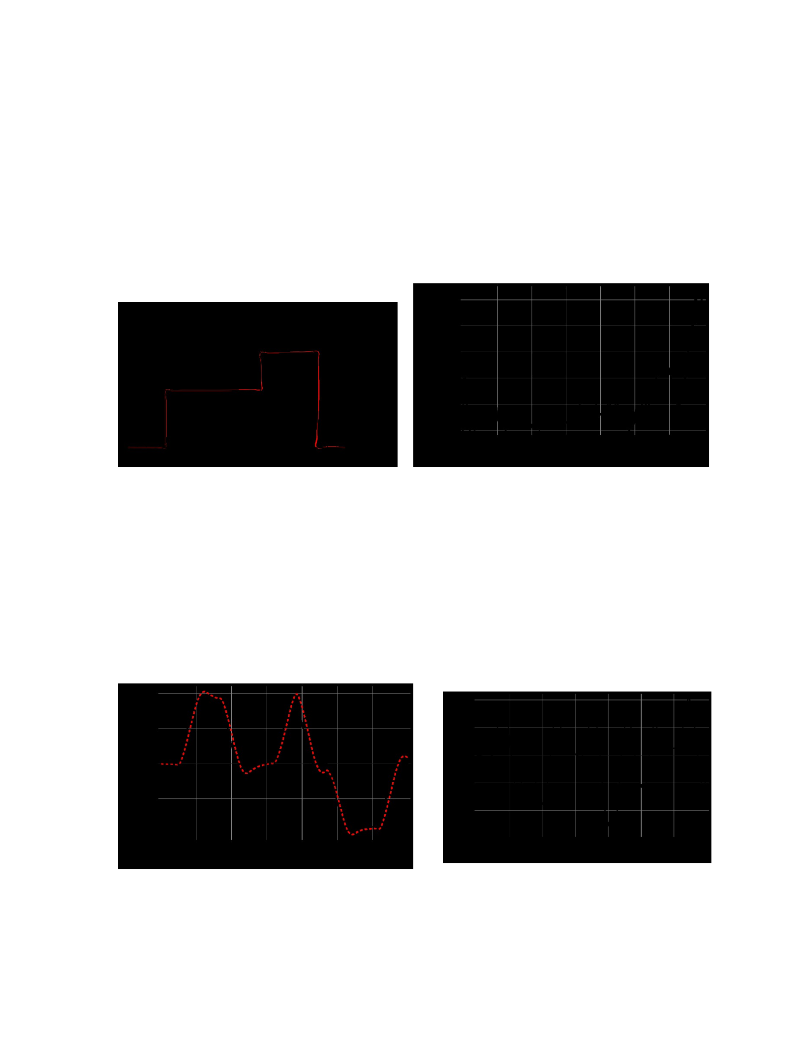
140

Simulation 1 requires the RoboBoat to maintain the direction of the tangent line, using a 5-

second forward look time. The results of this simulation are illustrated in the parametric plot

shown in Figure [25], which compares the desired and actual trajectories of the ship. Position

deviations, exy, during this operation are presented in Figure [26], providing a quantitative

assessment of the ship's position deviations.

Figure 25: Simulation 1 Parametric Plot Figure 26: Simulation 1 Position Deviation

Plot exy

The RoboBoat's ability to execute the direction of the path tangent for track 1, as shown in

simulation 1, is shown in Figure [24], where the desired and actual direction of the

RoboBoat is plotted. Figure [28] shows the heading error, eψ of RoboBoat for simulation 1.

Figure 27: Simulation of 1 Title ψ Perfor-

mance Plot Figure 28: Simulation 1 Heading Error

Plot ψxy

141

Simulation 2 requires RoboBoat to track arbitrarily predetermined titles,

11.459t

0.055T2 degrees. The results of this simulation are illustrated in the

parametric plot shown in Figure [29], which compares the desired and actual direction of

the ship. The heading error, e, during this operation is presented in Figure [30], providing a

quantitative assessment of the ship's heading control.

Figure 29: Simulation of 2 Parametric Plots Figure 30: Simulation 2 Misalignment

Plot exy

The RoboBoat's ability to control directional and planar movements simultaneously, as

shown in simulation 2, is shown in Figure [31], where the desired and actual direction of the

RoboBoat is plotted. Figure [32] shows the heading error, eψ from RoboBoat for simulation

Figure 31: Simulation of 2 Titles ψ Perfor-

Plot mance Figure 32: Simulation 2 Heading Errors eψ Plot

142

RoboBoat track tracking performance for track 1 is summarized in Table

Table 9: Track 1: Simulation Results 1 & 2

Simulation Path Error |exy| [m] Title Error |eψ| [◦]

Tengah Max Min RMSE Tengah

1 0.020 0.107 0.000 0.027 8.64

2 0.030 0.054 0.000 0.028 1.21

From Table 9, the results of simulations 1 and 2 show the effective mitigation of the

phenomenon of path cutting, a common problem in the line of sight guidance system when

dealing with geometry such as the one in Track 1, for both operations involving path tangent

heading and arbitrary heading.

8.2 Track 2: Simulation 3 (Lemniscate Figure-8)

Track 2 follows the lemniscate pattern, or number eight, and has a duration of 135 seconds.

This track is a standard benchmark for assessing the performance of autonomous vehicles. In

Simulation 3, the conventional navigation approach along this trajectory is modified by

incorporating control of the wobble motion around the curvature of the figure eight. This is

achieved by extending the time to look ahead, promoting the RoboBoat to adjust its direction

before the turn approaches. This approach induces a controlled side slip movement,

temporarily aligning the ship's movement with its sway axis. The simulation investigates the

capabilities of a proposed guiding strategy to facilitate RoboBoat movement in events

involving dynamic coupling between several degrees of freedom.

Simulation 3 is carried out under the following conditions, resulting from the temporal

143

Obstacles imposed by track 2:

•Average speed: 1,144 m/s

•Maximum speed: 1,642 m/s

•Minimum speed: 0.808 m/s

Figure [33] illustrates the external interference force exerted on the RoboBoat during

simulation 3.

Figure 33: Simulation of 3 External Disturbance Forces

Simulation 3 required the RoboBoat to maintain the direction of the tangent of the path,

using an 11-second forward looking time. The results of this simulation are illustrated in the

parametric plot shown in Figure [34], which compares the desired and actual trajectory of

the RoboBoat. The position deviation, exy, during this operation is presented in Figure [35],

providing a quantitative assessment of the RoboBoat's position deviation.

144

Figure 34: Simulated Parametric Plot 3

Figure 35: Simulation of 3 Position Deviations

Plot exy

The RoboBoat's ability to maintain the direction of the tangent path, as shown in simulation

3, is shown in Figure [36], where the desired and actual direction of the RoboBoat is plotted.

Figure

[37] displays a title error, eψ from RoboBoat for simulation 3.

Figure 36: Simulation of 3 Titles ψ Perfor-

mance Plot

Figure 37: Simulation of 3 eψ Title Error

Plot

Figures [35] and [37] show RoboBoat's ability to track a figure-8 trajectory involving

swaying motion control, while achieving the desired path tangent direction requirements.

RoboBoat's track tracking performance for track 2 is summarized in Table 10.

145

Table 10: Track 2: Simulation Results 3

Simulation Path Error |exy| [m] Title Error |eψ| [◦]

Average Max Min RMSE Middle

3 0.115 0.358 0.000 0.114 0.72

The results from simulation 3, Table 10, show RoboBoat's ability to perform proper

path compliance for paths involving lemniscate geometry.

8.3 Track 3: Simulation 4 & 5 (Circular)

Track 3 is formulated to evaluate the trajectory tracking performance of RoboBoat through

simulations 4 and 5, focusing on controlling the direction of the tangent path in the

environment with an increase in water current velocity of 0.318 m/s. This represents an

increase of about 50% compared to the current previous simulation speed. Furthermore, in

simulation 5, the RoboBoat's capacity to handle thruster errors was effectively demonstrated.

It exemplifies the fault-tolerant capabilities of an overdriven-driven system by requiring the

RoboBoat to navigate a circular path despite losing a single thruster. Track 3 has a time

duration of 300 seconds.

Simulations 4 and 5 were performed under the following conditions, resulting from the

temporal constraints imposed by trajectory 3:

•Average speed: 0.800 m/s

•Maximum speed: 0.984 m/s

•Minimum speed: 0.547 m/s

Figure [38] illustrates the random external interference force given to the RoboBoat during

simulations 4 and 5.

146

Figure 38: Simulation of 4 and 5 External Interference Forces

Simulation 4 requires the RoboBoat to maintain the direction of the tangent of the path, using

the time seen forward 1 second. The results of this simulation are illustrated in the parametric

plot shown in Figure [39], which compares the desired and actual trajectory of the RoboBoat.

The position deviation, exy, during this operation is presented in Figure [40], providing a

quantitative assessment of the RoboBoat position deviation.

Figure 39: Simulation of 4 Parametric

Plots

Figure 40: Simulation of 4 Position Deviations

Plot exy

RoboBoat's ability to control heading and planar movements simultaneously, as shown in

simulation 4, is shown in Figure [41], where the heading is desired and actual

147

RoboBoat plotted. Figure [42] shows the heading error, eψ from RoboBoat for simulation 4.

Figure 41: Simulation of 4 Titles ψ Perfor-

mance Plot Figure 42: Simulation of 4 eψ Title Error

Plot

Simulation 5 requires the RoboBoat to maintain the tangent lane direction, using a 1 second

forward look-forward time, with thruster 1 considered inoperative, then Ft1

0. The results

of this simulation are illustrated in the parametric plot shown in Figure [43], which compares

the desired and actual trajectory of the RoboBoat. The position deviation, exy, during this

operation is presented in Figure [44], providing a quantitative assessment of the RoboBoat's

position deviation.

The RoboBoat's ability to simultaneously control directional and planar movements, as

shown in simulation 5, is shown in Figure [45], where the desired and actual direction of the

RoboBoat is plotted. Figure [46] shows the heading error, eψ of RoboBoat for simulation 5.

Simulation 4 demonstrates RoboBoat's ability to maintain track tracking along a circular

path under conditions of increased current velocity, while following the direction of the

tangent of the path. Under the same environmental conditions and the desired direction,

simulation 5

148

Figure 43: Simulation of 5 Parametric

Plots

Figure 44: Simulation of 5 Position Deviations

Plot exy

Figure 45: Simulation of 5 Titles ψ Perfor-

Plot mance Figure 46: Simulation of 5 Heading Errors eψ

Plot

demonstrating RoboBoat's trajectory tracking capabilities despite the loss of actuator

functionality. The RoboBoat trajectory tracking performance under these conditions for track

3 is summarized in Table 11.

The results of simulations 4 and 5, Table 11, The results show that the RoboBoat

successfully maintains proper adherence to the circular trajectory, effectively compensates

for heading discontinuities in the control framework and adequately handles current increases

and actuator failures. These findings show over-driven sturdiness

149

Table 11: Track 3: Simulation Results 4 & 5

Simulation Path Error |exy| [m] Title Error |eψ| [◦]

Tengah Max Min RMSE Tengah

4 0.181 0.549 0.000 0.118 0.76

5 0.261 0.539 0.000 0.189 0.83

its configuration and ability to work reliably in more challenging operational conditions.

8.4 Track 4: Simulation 6 & 7 (Concentric)

Track 4 evaluates the RoboBoat's trajectory tracking performance under the challenges posed

by the circular path, which introduces discontinuity in the control framework as the desired

direction exceeds the 180-degree ± range of the arctan2 function. This constraint tests the

controller's ability to maintain smooth path following behavior, especially during rapid or

significant changes in direction. Simulation 6 focuses on RoboBoat's ability to align with the

tangent line of the path along a circular trajectory, ensuring the absolute direction is mapped

into a continuous span to prevent incorrect control actions. Simulation 7 required the same

operation as the one in simulation 6 with an initial offset introduction of 0.27 m to analyze

the fault mitigation and recovery behavior of the ship. This simulation evaluates the effects

of additional integrators in the control structure, which, while effective in eliminating steady-

state errors, increases sensitivity to early conditions. This sensitivity can lead to transient

behaviors, such as overshoot or extended recovery times, which are critical to analyzing for

real-world implementations. Track 4 has a time duration of 200 seconds.

Simulations 6 and 7 were performed under the following conditions, resulting from

temporal constraints imposed by trajectory 4:

150

•Average speed: 0.728 m/s

•Maximum speed: 0.779 m/s

•Minimum speed: 0.671 m/s

Figure [47] illustrates the random external interference force exerted on the RoboBoat

during simulations 6 and 7.

Figure 47: Simulation of 6 and 7 External Interference Forces

Simulation 6 requires the RoboBoat to maintain the direction of the tangent of the path, using

a 4-second forward look time. The results of this simulation are illustrated in the parametric

plot shown in Figure [48], which compares the desired and actual trajectory of the RoboBoat.

The position deviation, exy, during this operation is presented in Figure [49], providing a

quantitative assessment of the RoboBoat's position deviation.

151

Figure 48: Simulated Parametric Plot 6

Figure 49: Simulation of 6 Position Deviations

Plot exy

The RoboBoat's ability to control directional and planar movements simultaneously, as

shown in simulation 6, is shown in Figure [50], where the desired and actual direction of the

RoboBoat is plotted. Figure [51] shows the heading error, eψ of RoboBoat for simulation 6.

Figure 50: Simulation of 6 Titles ψ Perfor-

mance Plot

Figure 51: Simulation of 6 Title Error eψ

Plot

Simulation 7 required the RoboBoat to maintain the direction of the tangent of the path, using

a look-ahead time of 4 seconds, with an initial offset of -0.25m and 0.1m in the x and y

directions, respectively. The results of this simulation are illustrated in the parametric plot

shown in

152

Figure [52], which compares the desired and actual RoboBoat trajectories. Position

deviations, e, during this operation are presented in Figure [53], providing a quantitative

assessment of the RoboBoat position deviation.

Figure 52: Simulated Parametric Plot 7

Figure 53: Simulation of 7 Position Deviations

Plot exy

The RoboBoat's ability to control directional and planar movements simultaneously, as

shown in simulation 7, is shown in Figure [54], where the desired and actual direction of the

RoboBoat is plotted. Figure [55] shows the heading error, eψ of RoboBoat for simulation 7.

Figure 54: Simulation of 7 Titles ψ Perfor-

Plot mance Figure 55: Simulation of 7 Heading Errors eψ

Plot

153

The trajectory tracking performance of RoboBoat for simulations 6 and 7, under the

conditions discussed for track 4 is summarized in Table 12.

Table 12: Track 4: Simulation Results 6 & 7

Simulation Path Error |exy| [m] Title Error |eψ| [◦]

Middle Max Min RMSE Middle

6 0.055 0.163 0.000 0.046 0.28

7 0.114 0.223 0.002 0.094 0.31

The results of simulations 6 and 7, presented in Table 12, demonstrate RoboBoat's ability to

achieve precise path compliance along a circular trajectory. The controller effectively

handles the desired heading mapping to avoid discontinuities and erroneous control actions

caused by the arctan2 function, while demonstrating strong performance in eliminating errors

arising from the initial offset condition.

8.5 Track 5: Simulation 8 & 9 (Straight Line)

Track 5 evaluates the RoboBoat track tracking performance along a straight line path. In

simulations 8 and 9, RoboBoat demonstrated its ability to perform diagonal movements

along a straight track while simultaneously controlling its direction. Simulation 8 requires

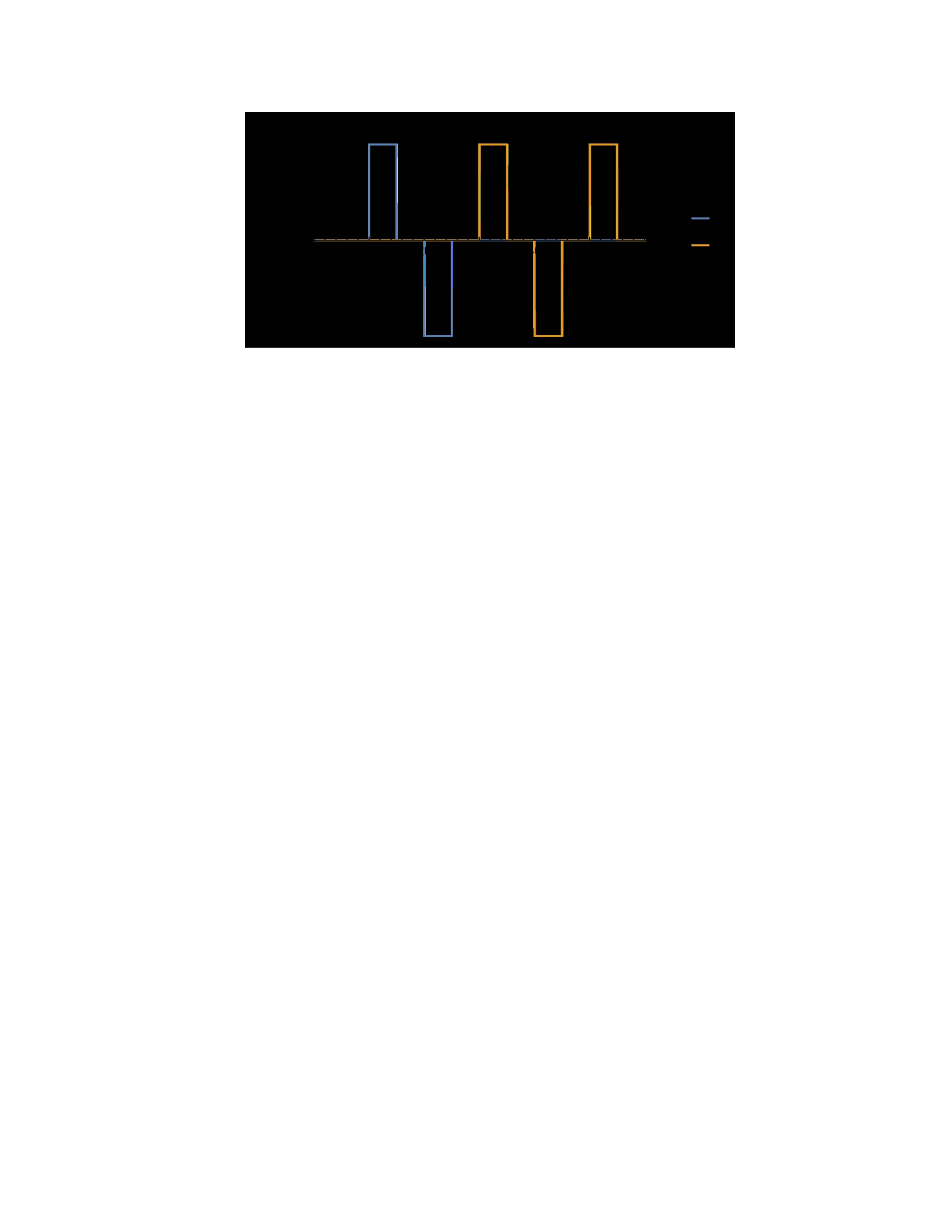
154

Figure 56: Simulation of 8 and 9 External Interference Forces

RoboBoat to maintain a fixed direction of 0 ◦while navigating a diagonal path, while

simulation 9 assigns the ship to follow a predetermined arbitrary direction while following

the same trajectory. The simulation highlights the RoboBoat's Omnidirectional capabilities,

demonstrating its ability to independently control movement across all degrees of its

freedom.

Track 5 has a time duration of 60 seconds.

Simulations 8 and 9 were performed under the following conditions, resulting from

temporal constraints imposed by trajectory 5:

•Average speed: 0.692 m/s

•Maximum speed: 1.06 m/s

•Minimum speed: 0.300 m/s

Figure [56] illustrates the random external interference force exerted on the RoboBoat during

simulations 8 and 9. The trajectory tracking performance of RoboBoat for simulation 8 is

illustrated in a parametric plot, Figure [57], which compares the desired and actual ship

trajectories. The position deviation, exy, during this operation is presented in Figure [58],

155

providing a quantitative assessment of RoboBoat's performance.

156

Figure 58: Simulation of 8 Position Deviations

Plot exy

Figure 57: Simulation of 8 Parametric Plots

The RoboBoat's ability to maintain a direction of 0◦ (direction nˆ1), while traversing a

diagonal path positioned at 45 ◦(relative to direction nˆ1), as shown in simulation 8, is

shown in Figure [59], where the desired and actual direction of the RoboBoat is plotted.

Figure [60] shows the heading error, eψ of RoboBoat for simulation 9.

Figure 59: Simulation of 8 titles ψ Perfor-

mance plot. Figure 60: Simulation of 8 Title Error eψ

Plot

Simulation 9 requires RoboBoat to track an arbitrarily predetermined title, ψd

0.16t2

degrees. The results of this simulation are illustrated in the parametric plot shown in Figure

[61], which compares the desired and actual direction of the ship. Heading error, exy, during

157

This operation is presented in Figure [62], providing a quantitative assessment of the ship's

direction control.

Figure 62: Simulation of 9 Position Deviations

Plot exy

Figure 61: Simulated Parametric Plot 9

The RoboBoat's ability to control directional and planar movements simultaneously, as

shown in simulation 9, is shown in Figure [63], where the desired and actual direction of the

RoboBoat is plotted. Figure [64] shows the heading error, eψ of RoboBoat for simulation 9.

Figure 63: Simulation of 9 Titles ψ Perfor-

mance Plot Figure 64: Simulation of 9 Title Error eψ Plot

158

RoboBoat's track tracking performance for track 5 is summarized in Table 13.

Table 13: Results of Path 5 Simulation

Simulation No. Path Error |exy| [m] Title Error |eψ| [◦]

Middle Max Min RMSE Middle

8 0.079 0.184 0.000 0.035 0.26

9 0.019 0.062 0.000 0.018 1.32

Table 13 presents the results of simulations 8 and 9, showing the RoboBoat's effective

independent control of the degrees of freedom of x, y, and ψ. RoboBoat successfully

performs track tracking control while maintaining a fixed direction and the desired variety

of directions along a straight-line trajectory, demonstrating its precise and versatile control

capabilities.

159

9 Closing Remarks

9.1 Conclusion

Autonomous navigation systems represent advances in modern technology, characterized by

their ability to perform complex tasks in dynamic and uncertain environments. The

increasing implementation of autonomous navigation systems requires the formulation of a

robust and reliable control system, which requires a comprehensive understanding and

representation of the system dynamics, which accurately represents the

real-world behavior, combining physical principles, environmental interactions, and

operational constraints.

This research focuses on the development of dynamic models with high precision and

a trajectory tracking control framework based on the physical nature and capabilities of an

over-maneuvered autonomous surface vessel, RoboBoat. The study systematically addresses

the complexities of omnidirectional dynamics, actuator redundancy, and combined control of

different degrees of freedom to ensure a more authentic representation of vessel behavior and

provide reliable insights into system performance under realistic operational conditions.

The dynamic model of six degrees of freedom, derived using the Kane method, provides an

accurate representation of the ship's behavior, taking into account combined motion,

nonlinear attenuation, and environmental interactions. The pseudo-physical system

identification approach streamlines the modeling process, eliminating the need for extensive

empirical testing. The control strategy combines an integrated decentralized proportional-

integral-derivative controller with a line of sight. Pseudo-inverse-based thrust allocation

160

An algorithm is used to resolve the redundancy inherent in the x-configured RoboBoat

propulsion system, ensuring effective thrust distribution across multiple actuators.

The findings of this study demonstrate the robustness and efficacy of the developed high-

fidelity dynamic model and trajectory tracking control framework for over-driven

autonomous surface ships. The simulation evaluates the system in a variety of trajectory

scenarios, including high curvature paths, intermittent direction changes, and

omnidirectional maneuvers. The proposed control strategy, found to effectively address

the challenges of omnidirectional dynamics, actuator redundancy, and

multi-degree control of freedom. The undercutting phenomenon often encountered in the

line-of-sight guide is reduced through the application of dynamic look-ahead time instead

of a fixed look-ahead distance, improving the adaptability of the guide strategy for various

operational conditions. In addition, the system demonstrates the ability to maintain a

strong station in a dynamic environment. Quantitative metrics, such as

Track errors and directional deviations, confirming the system's ability to ensure path

compliance with minimal deviations.

9.2 Future Jobs

Future research should focus on experimental validation of dynamic models and control

strategies through sea trials to further assess real-world performance. Incorporating

adaptive or machine learning-based control algorithms can increase resilience to unmodeled

dynamics and environmental variability. Extending the methodology to larger vessels or

multi-ship coordination will expand its application, supporting advances in

maritime operations and autonomous navigation systems.

ADVANCED DYNAMIC MODELING AND TRAJECTORY-TRACKING CONTROL OF AN OVERACTUATED AUTONOMOUS SURFACE VESSEL

Students also viewed