


MAT 275 MATLAB Lab 6
Exercise 1
function LAB06ex1
clc
omega0 = 2; c = 1; omega = 1.4;
param = [omega0,c,omega];
t0 = 0; y0 = 0; v0 = 0; Y0 = [y0;v0]; tf = 50;
options = odeset('AbsTol',1e-10,'relTol',1e-10);
[t,Y] = ode45(@f,[t0,tf],Y0,options,param);
y = Y(:,1); v = Y(:,2);
figure(1)
plot(t,y,'b-'); ylabel('y'); grid on;
t1 = 25; i = find(t>t1);
C = (max(Y(i,1))-min(Y(i,1)))/2;
disp(['computed amplitude of forced oscillation = ' num2str(C)]);
Ctheory = 1/sqrt((omega0^2-omega^2)^2+(c*omega)^2);
disp(['theoretical amplitude = ' num2str(Ctheory)]);
end
%----------------------------------------------------------------
function dYdt = f(t,Y,param)
y = Y(1); v = Y(2);
omega0 = param(1); c = param(2); omega = param(3);
dYdt = [ v ; cos(omega*t)-omega0^2*y-c*v ];
end
% The output of this function file display in the command window
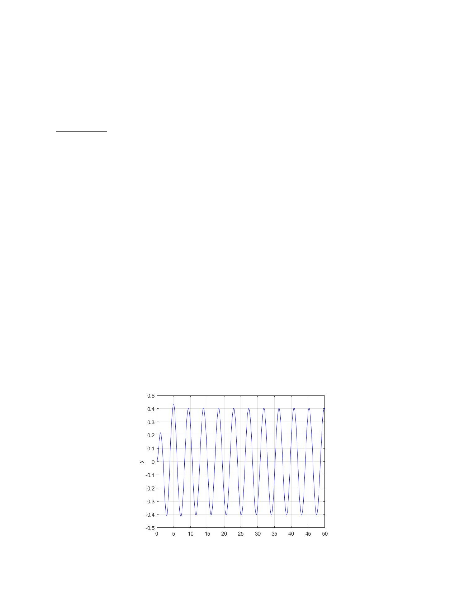
computed amplitude of forced oscillation = 0.40417
theoretical amplitude = 0.40417
% The graphical output
(a)
The period of the forced oscillation can be determined by calculating
T=2π
ω
where ω = 1.4 according to the initial conditions
T=2π
ω=2π
1.4 ≈4.49
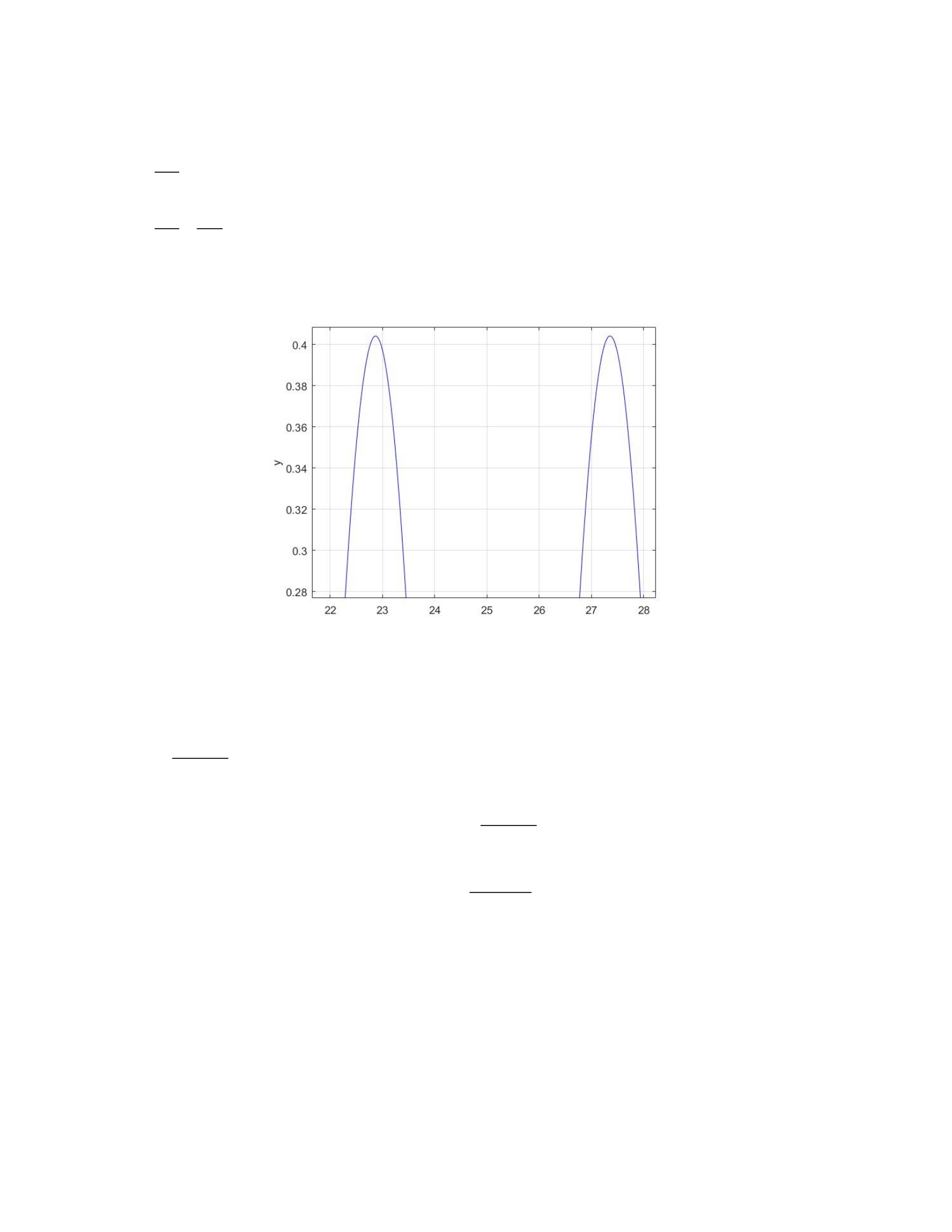
This can be verified by observing the distance between two peaks of
the graph above
The first peak is at about 22.9 and the second peak is at about 27.3,
the distance between the peaks is 27.3-22.9=4.4 which is approximately
what was calculated above. This helps to verify our calculations.
The numerical value of the angle α would be calculated using
tan−1
(
cω
ω0
2−ω2
)
since
ω0>ω
α=tan−1
(
cω
ω0
2−ω2
)
¿tan−1
(
1∗1.4
22−1.42
)
≈34.5° ≈ 0.601 radians

(b)
function LAB06ex1
clc
omega0 = 2; c = 1; omega = 1.4;
param = [omega0,c,omega];
t0 = 0; y0 = 0; v0 = 0; Y0 = [y0;v0]; tf = 50;
options = odeset('AbsTol',1e-10,'relTol',1e-10);
[t,Y] = ode45(@f,[t0,tf],Y0,options,param);
y = Y(:,1); v = Y(:,2);
figure(1)
plot(t,y,'b-'); ylabel('y'); grid on;
t1 = 25; i = find(t>t1);
C = (max(Y(i,1))-min(Y(i,1)))/2;
disp(['computed amplitude of forced oscillation = ' num2str(C)]);
Ctheory = 1/sqrt((omega0^2-omega^2)^2+(c*omega)^2);
disp(['theoretical amplitude = ' num2str(Ctheory)]);
% The following lines are the added lines to compute yc and graph it
alpha=atan(c*omega/(omega0^2-omega^2)); % computes alpha
yc=y-Ctheory*cos(omega*t-alpha); % computes yc
figure(2) % opens new figure
plot(t,yc,'b-'); grid on; title('complementary solution'); % plots yc
end
%----------------------------------------------------------------
function dYdt = f(t,Y,param)
y = Y(1); v = Y(2);
omega0 = param(1); c = param(2); omega = param(3);
dYdt = [ v ; cos(omega*t)-omega0^2*y-c*v ];
end
% The output produces the same results as the original file with an
added graph representing the oscillation of the complementary solution
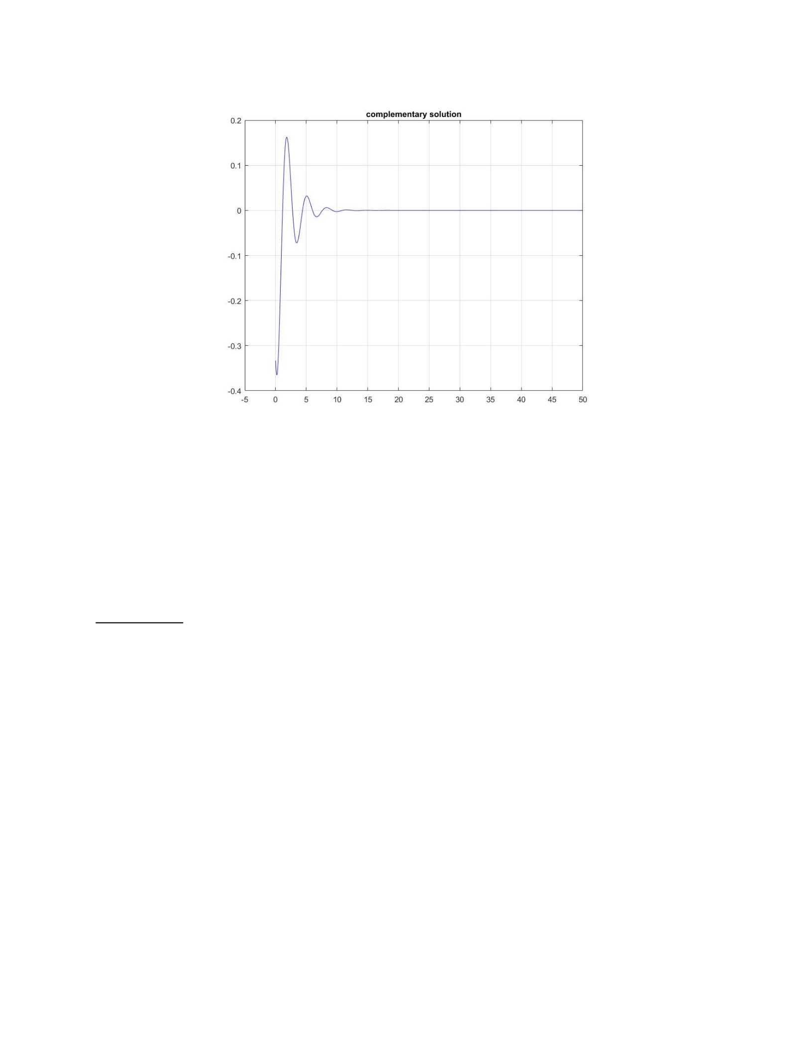
I extended the x axis to begin less than zero to view the
complete graph.
This looks like an exponentially decreasing oscillation because
the first oscillation is close to the 0.4 amplitude as expected from
the original but as t increases, the oscillation diminishes rapidly to
zero. The oscillation reaches zero and stays there at about t=10 which
makes sense because the particular solution (yp) stabilizes at about
this point. The complementary solution is also known as the transient
solution because it dies out over time which is represented by the
above graph.
Exercise 2
(a)
function LAB06ex2
omega0 = 2; c = 1;
OMEGA = 1:0.02:3;
C = zeros(size(OMEGA));
Ctheory = zeros(size(OMEGA));
t0 = 0; y0 = 0; v0 = 0; Y0 = [y0;v0]; tf = 50; t1 = 25;
for k = 1:length(OMEGA)
omega = OMEGA(k);
param = [omega0,c,omega];
[t,Y] = ode45(@f,[t0,tf],Y0,[],param);
i = find(t>t1);
C(k) = (max(Y(i,1))-min(Y(i,1)))/2;
% The equation for C or the amplitude is entered here
Ctheory(k) = 1/sqrt((omega0^2-omega^2)^2+(c*omega)^2);
end
figure(2)
% we want to plot The theoretical and computed values of C vs ω
plot(OMEGA,C,OMEGA,Ctheory,'ro'); grid on;
xlabel('\omega'); ylabel('C');
end
%---------------------------------------------------------
function dYdt = f(t,Y,param)
y = Y(1); v = Y(2);
omega0 = param(1); c = param(2); omega = param(3);
dYdt = [ v ; cos(omega*t)-omega0^2*y-c*v ];
end
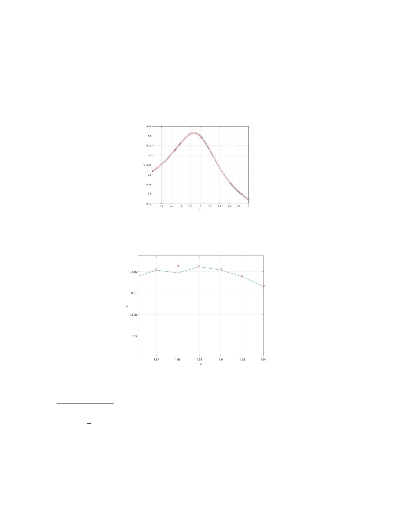
% The output graph from the function file
(b)
When C is maximum, ω is approximately 1.87, this value is the
practical resonance frequency. The corresponding maximum value for C
is approximately 0.517.
(c)
To find the practical resonance frequency analytically we can
differentiate the following equation as a function of ω.
ω
√
(¿¿02−ω2)2+c2ω2
C=1
¿

ω
(¿¿02−ω2)2
¿
¿
+c2
∗d
dω
[
ω2
]
¿
ω
(¿¿02−ω2)2+c2ω2
¿
¿
¿
d
dω ¿
dC
dω=−¿
Simplify
c2−2ω
ω
(¿¿02−ω2)2+c2ω2
¿
¿
¿
¿
2ω3+ω(¿¿02)
¿
dC
dω=−¿
Set
dC
dω=0
and solve for ω
c2−2ω
ω
(¿¿02−ω2)2+c2ω2
¿
¿
¿
¿
2ω3+ω(¿¿02)
¿
0=−¿
There are three solutions for ω
ω=0
ω=−
√
c2−2ω0
2
√
2

ω=
√
c2−2ω0
2
√
2
The actual solution will be the third option
Enter values for c and
ω0
❑
ω=
√
12−2∗2❑
2
√
2=1.871i
This value is complex but the numerical value is very close to the
estimated value of ω in part b.
(d)
function LAB06ex1
clc
omega0 = 2; c = 1; omega = 1.871;
param = [omega0,c,omega];
t0 = 0; y0 = 0; v0 = 0; Y0 = [y0;v0]; tf = 50;
options = odeset('AbsTol',1e-10,'relTol',1e-10);
[t,Y] = ode45(@f,[t0,tf],Y0,options,param);
y = Y(:,1); v = Y(:,2);
figure(1)
plot(t,y,'b-'); ylabel('y'); grid on;
t1 = 25; i = find(t>t1);
C = (max(Y(i,1))-min(Y(i,1)))/2;
disp(['computed amplitude of forced oscillation = ' num2str(C)]);
Ctheory = 1/sqrt((omega0^2-omega^2)^2+(c*omega)^2);
disp(['theoretical amplitude = ' num2str(Ctheory)]);
alpha=atan(c*omega/(omega0^2-omega^2));
yc=y-Ctheory*cos(omega*t-alpha);
figure(2)
plot(t,yc,'b-'); grid on; title('complementary solution');
end
%----------------------------------------------------------------
function dYdt = f(t,Y,param)
y = Y(1); v = Y(2);
omega0 = param(1); c = param(2); omega = param(3);
dYdt = [ v ; cos(omega*t)-omega0^2*y-c*v ];
end
% Output of the fuction file
computed amplitude of forced oscillation = 0.5164
theoretical amplitude = 0.5164

The
theoretical/computed amplitude both show
0.5164, while looking at the graph it looks like it is around 0.5 so
this checks out. This amplitude is larger than the result from
question 1. If the program is ran with any other value of ω then the
amplitude will be smaller. The value of 1.871 is the resonant
frequency and this should yield the largest amplitude so using any
other value would yield a smaller amplitude.
(e)
No matter what the initial conditions of y0 and v0, the output of this
function remains the same
function LAB06ex2
omega0 = 2; c = 1;
OMEGA = 1:0.02:3;
C = zeros(size(OMEGA));
Ctheory = zeros(size(OMEGA));
t0 = 0; y0 = 23; v0 = 67; Y0 = [y0;v0]; tf = 50; t1 = 25;
for k = 1:length(OMEGA)
omega = OMEGA(k);
param = [omega0,c,omega];
[t,Y] = ode45(@f,[t0,tf],Y0,[],param);
i = find(t>t1);
C(k) = (max(Y(i,1))-min(Y(i,1)))/2;
Ctheory(k) = 1/sqrt((omega0^2-omega^2)^2+(c*omega)^2);
end
figure(2)
plot(OMEGA,C,OMEGA,Ctheory,'ro'); grid on;
xlabel('\omega'); ylabel('C');
end
%---------------------------------------------------------
function dYdt = f(t,Y,param)
y = Y(1); v = Y(2);
omega0 = param(1); c = param(2); omega = param(3);
dYdt = [ v ; cos(omega*t)-omega0^2*y-c*v ];
end
% Output graph
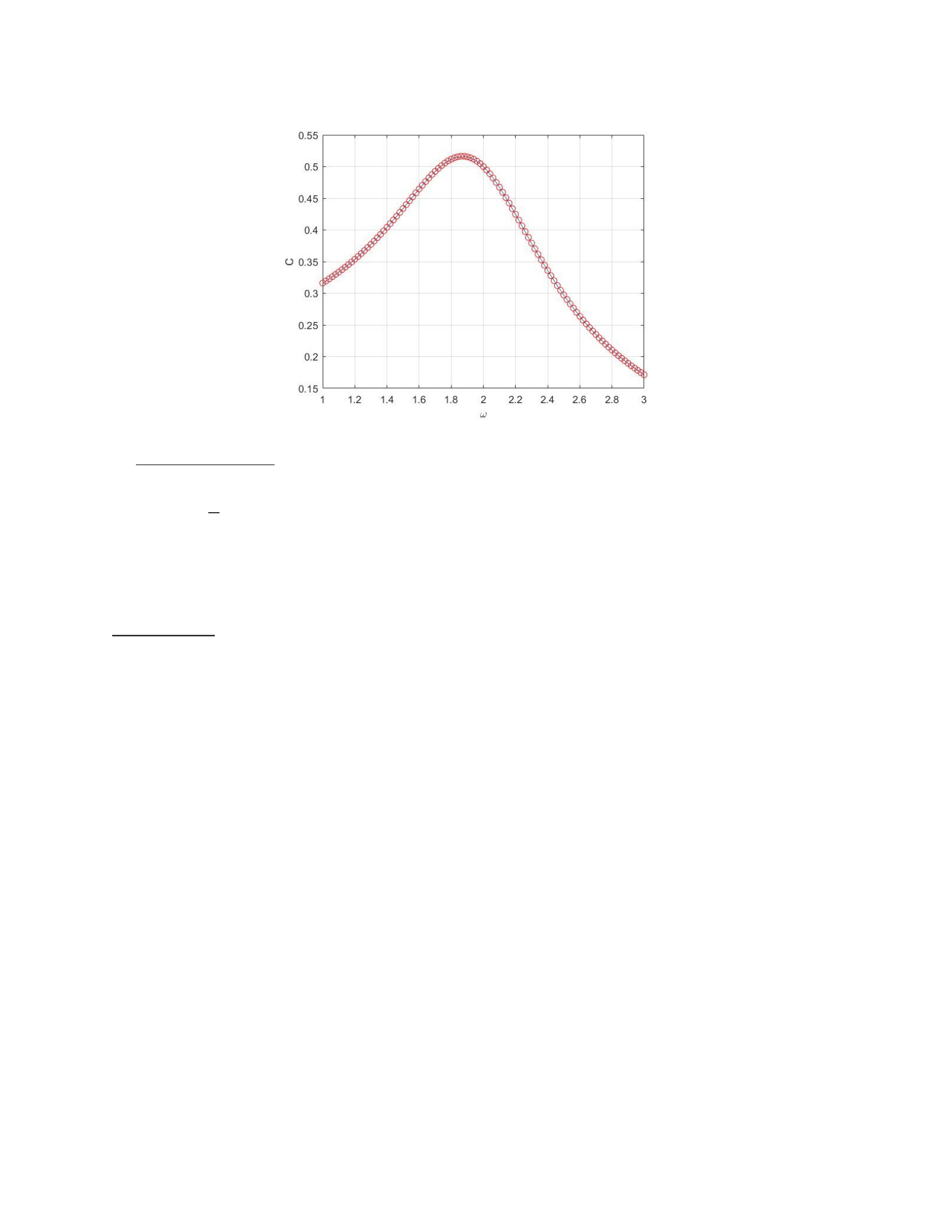
By using the expression L6.3 for C;
ω
√
(¿¿02−ω2)2+c2ω2
C=1
¿
It is plain to see that since y0 and v0 are not in the
expression, they will not have an effect on the outcome.
Exercise 3
function LAB06ex2
omega0 = 2; c = 0;
OMEGA = 1:0.02:3;
C = zeros(size(OMEGA));
Ctheory = zeros(size(OMEGA));
t0 = 0; y0 =0; v0 = 0; Y0 = [y0;v0]; tf = 50; t1 = 25;
for k = 1:length(OMEGA)
omega = OMEGA(k);
param = [omega0,c,omega];
[t,Y] = ode45(@f,[t0,tf],Y0,[],param);
i = find(t>t1);
C(k) = (max(Y(i,1))-min(Y(i,1)))/2;
Ctheory(k) = 1/sqrt((omega0^2-omega^2)^2+(c*omega)^2);
end
figure(2)
plot(OMEGA,C,OMEGA,Ctheory,'ro'); grid on;
xlabel('\omega'); ylabel('C');
end
%---------------------------------------------------------
function dYdt = f(t,Y,param)
y = Y(1); v = Y(2);
omega0 = param(1); c = param(2); omega = param(3);
dYdt = [ v ; cos(omega*t)-omega0^2*y-c*v ];
end
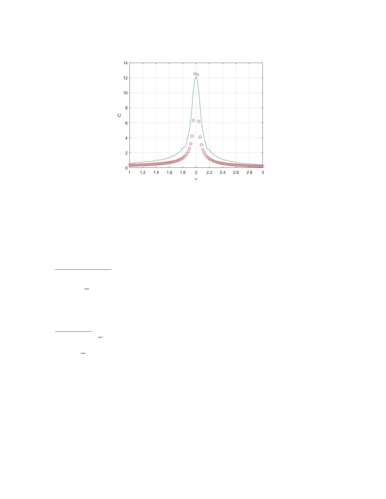
% Output Graph
(a)
When c=0, then the system is considered not damped. This results
in a system that is at resonance which will yield the maximum
amplitude for the system. The maximal amplitude according to the graph
is approximately 12 for the computed (blue) solution, and approaching
infinity for the theoretical (red) solution. The value of ω
corresponding to the maximum amplitude is 2. This is the same value as
ω0. Which means as ω approaches ω0 then the maximum amplitude is
yielded.
When analyzing the equation for C:
ω
√
(¿¿02−ω2)2+c2ω2
C=1
¿
When c=0 then the equation becomes
ω
¿ω0
2−ω2∨¿
√
(¿¿02−ω2)2=1
¿
C=1
¿
Where it is plain to see that as ω approaches ω0, C will increase
exponentially.
(b)
function LAB06ex1
clc
omega0 = 2; c = 0; omega = 2;
param = [omega0,c,omega];
t0 = 0; y0 = 0; v0 = 0; Y0 = [y0;v0]; tf = 50;
options = odeset('AbsTol',1e-10,'relTol',1e-10);
[t,Y] = ode45(@f,[t0,tf],Y0,options,param);
y = Y(:,1); v = Y(:,2);
figure(1)
plot(t,y,'b-'); ylabel('y'); grid on;
%t1 = 25; i = find(t>t1);
%C = (max(Y(i,1))-min(Y(i,1)))/2;
%disp(['computed amplitude of forced oscillation = ' num2str(C)]);
%Ctheory = 1/sqrt((omega0^2-omega^2)^2+(c*omega)^2);
%disp(['theoretical amplitude = ' num2str(Ctheory)]);
%alpha=atan(c*omega/(omega0^2-omega^2));
%yc=y-Ctheory*cos(omega*t-alpha);
%figure(2)
%plot(t,yc,'b-'); grid on; title('complementary solution');
end
%----------------------------------------------------------------
function dYdt = f(t,Y,param)
y = Y(1); v = Y(2);
omega0 = param(1); c = param(2); omega = param(3);
dYdt = [ v ; cos(omega*t)-omega0^2*y-c*v ];
end
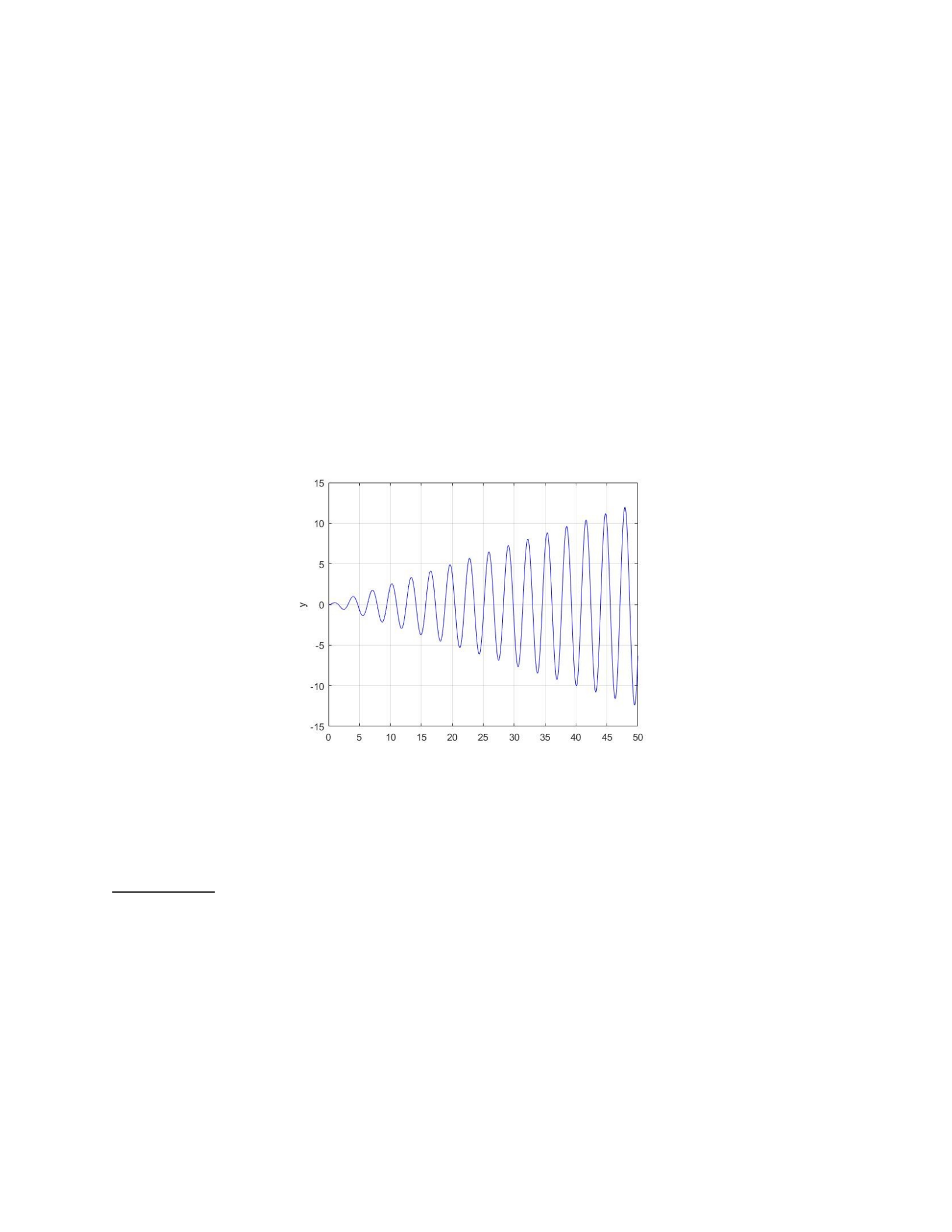
The amplitude of this solution is increasing and unbounded when ω
approaches ω0. The maximum amplitude in this graph is approximately 12
which corresponds with the graph’s amplitude in part 3.a. The behavior
of this system is still cyclical but because it is undamped, the
system’s amplitude can increase forever.
Exercise 4
function LAB06ex1
clc
omega0 = 2; c = 0; omega = 1.8;
param = [omega0,c,omega];
t0 = 0; y0 = 0; v0 = 0; Y0 = [y0;v0]; tf = 100;
options = odeset('AbsTol',1e-10,'relTol',1e-10);
[t,Y] = ode45(@f,[t0,tf],Y0,options,param);
y = Y(:,1); v = Y(:,2);
figure(1)
plot(t,y,'b-'); ylabel('y'); grid on;
%t1 = 25; i = find(t>t1);
%C = (max(Y(i,1))-min(Y(i,1)))/2;
%disp(['computed amplitude of forced oscillation = ' num2str(C)]);
%Ctheory = 1/sqrt((omega0^2-omega^2)^2+(c*omega)^2);
%disp(['theoretical amplitude = ' num2str(Ctheory)]);
%alpha=atan(c*omega/(omega0^2-omega^2));
%yc=y-Ctheory*cos(omega*t-alpha);
%figure(2)
%plot(t,yc,'b-'); grid on; title('complementary solution');
end
%----------------------------------------------------------------
function dYdt = f(t,Y,param)
y = Y(1); v = Y(2);
omega0 = param(1); c = param(2); omega = param(3);
dYdt = [ v ; cos(omega*t)-omega0^2*y-c*v ];
end
(a)
function LAB06ex1
clc
omega0 = 2; c = 0; omega = 1.8;
param = [omega0,c,omega];
t0 = 0; y0 = 0; v0 = 0; Y0 = [y0;v0]; tf = 100;
options = odeset('AbsTol',1e-10,'relTol',1e-10);
[t,Y] = ode45(@f,[t0,tf],Y0,options,param);
y = Y(:,1); v = Y(:,2);
figure(1)
plot(t,y,'b-'); ylabel('y'); grid on;
C=1/abs(omega0^2-omega^2);
A=2*C*sin((omega0-omega)*t/2);
hold on
plot(t,A,'r-',t,-A,'g-');
%t1 = 25; i = find(t>t1);
%C = (max(Y(i,1))-min(Y(i,1)))/2;
%disp(['computed amplitude of forced oscillation = ' num2str(C)]);
%Ctheory = 1/sqrt((omega0^2-omega^2)^2+(c*omega)^2);
%disp(['theoretical amplitude = ' num2str(Ctheory)]);
%alpha=atan(c*omega/(omega0^2-omega^2));
%yc=y-Ctheory*cos(omega*t-alpha);
%figure(2)
%plot(t,yc,'b-'); grid on; title('complementary solution');
end
%----------------------------------------------------------------
function dYdt = f(t,Y,param)
y = Y(1); v = Y(2);
omega0 = param(1); c = param(2); omega = param(3);
dYdt = [ v ; cos(omega*t)-omega0^2*y-c*v ];
end
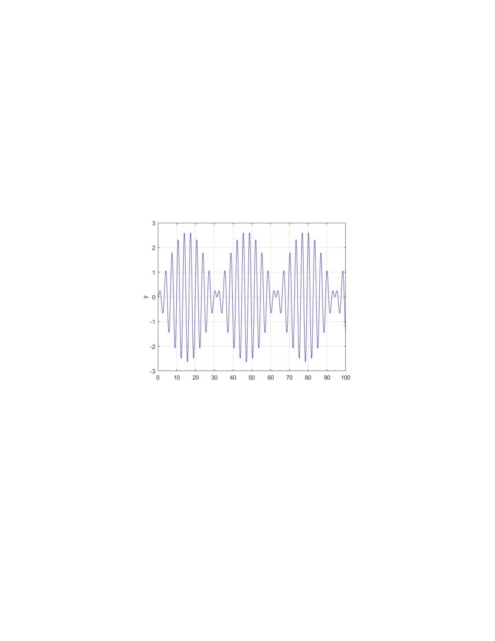
% Output Graph
(b)
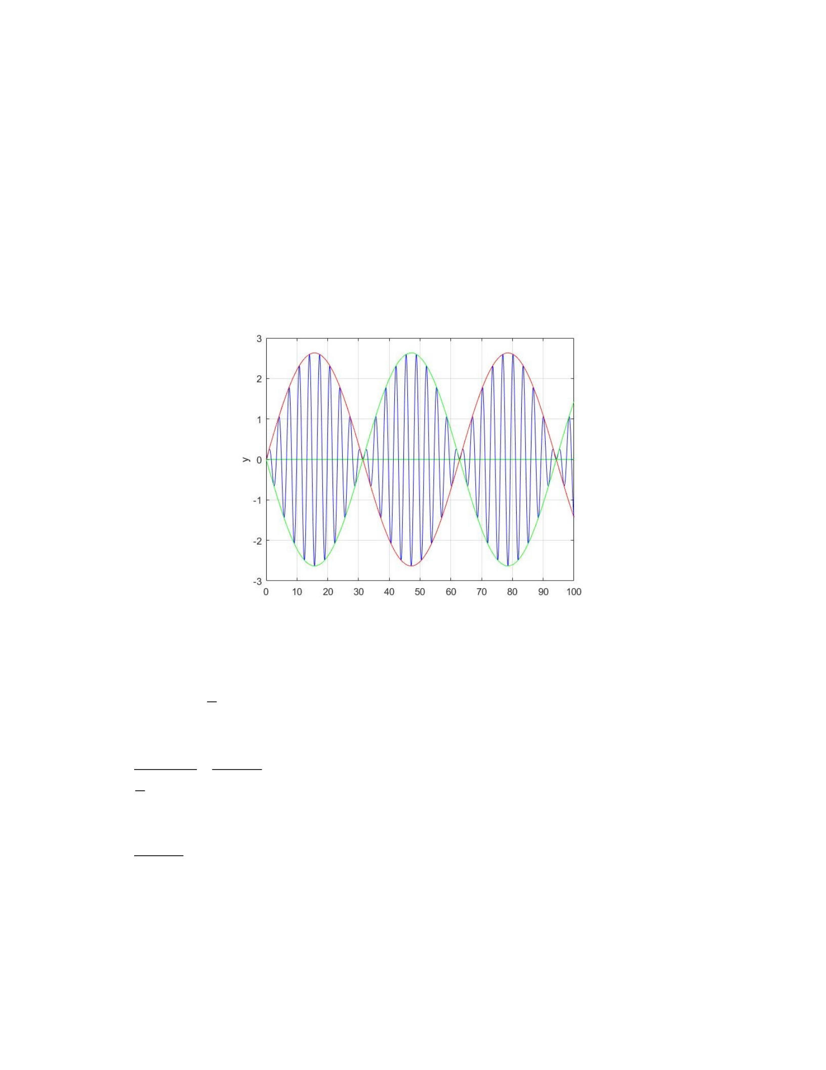
Analytically we can calculate the period of the fast oscillation y(t)
y
(
t
)
=A
(
t
)
sin
(
1
2
(
ω0+ω
)
t
)
Where the period is:
T=2π
1
2
(
ω0+ω
)
=4π
(
ω0+ω
)
Substitute in the given values:
T=4π
(
2+1.8
)
≈3.307
This value can be confirmed by zooming in on the distance of two peaks
on the graph and approximating the period
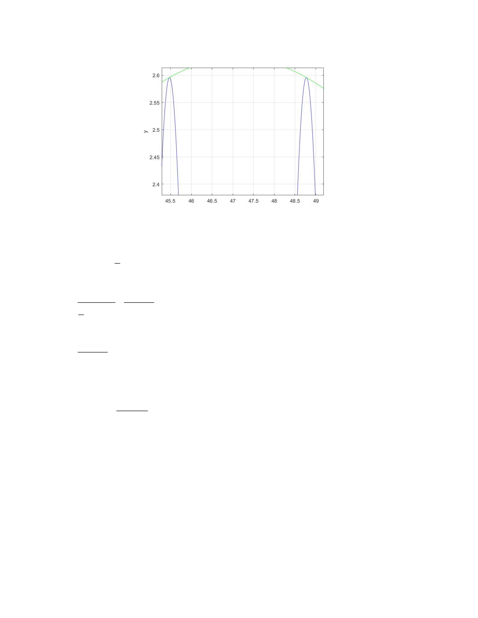
The first peak is at about 45.5 and the second at about 48.75 and the
difference is about 3.25 which is very close to our calculated period.
(c)
The length of the beat can be calculated by using:
A
(
t
)
=2Csin
(
1
2
(
ω0−ω
)
t
)
Where the period of this equation is
T=2π
1
2
(
ω0−ω
)
=4π
(
ω0−ω
)
Substitute in the given values
T=4π
(
2−1.8
)
≈62.8319
This value needs to be divided by two because there are two beats per
one period of the slow oscillation.
Therefore
Beat Length ≈ 62.8319
2≈31.4159
This value can be confirmed by zooming in on the point where the red
and green paths cross at half their period.

From the graph, the intersection is at about 31.4 or a little bigger,
which coincides with the calculated value.
(d)
function LAB06ex1
clc
omega0 = 2; c = 0; omega = 1.9;
param = [omega0,c,omega];
t0 = 0; y0 = 0; v0 = 0; Y0 = [y0;v0]; tf = 100;
options = odeset('AbsTol',1e-10,'relTol',1e-10);
[t,Y] = ode45(@f,[t0,tf],Y0,options,param);
y = Y(:,1); v = Y(:,2);
figure(1)
plot(t,y,'b-'); ylabel('y'); grid on;
C=1/abs(omega0^2-omega^2);
A=2*C*sin((omega0-omega)*t/2);
hold on
plot(t,A,'r-',t,-A,'g-');
%t1 = 25; i = find(t>t1);
%C = (max(Y(i,1))-min(Y(i,1)))/2;
%disp(['computed amplitude of forced oscillation = ' num2str(C)]);
%Ctheory = 1/sqrt((omega0^2-omega^2)^2+(c*omega)^2);
%disp(['theoretical amplitude = ' num2str(Ctheory)]);
%alpha=atan(c*omega/(omega0^2-omega^2));
%yc=y-Ctheory*cos(omega*t-alpha);
%figure(2)
%plot(t,yc,'b-'); grid on; title('complementary solution');
end
%----------------------------------------------------------------
function dYdt = f(t,Y,param)
y = Y(1); v = Y(2);
omega0 = param(1); c = param(2); omega = param(3);
dYdt = [ v ; cos(omega*t)-omega0^2*y-c*v ];
end
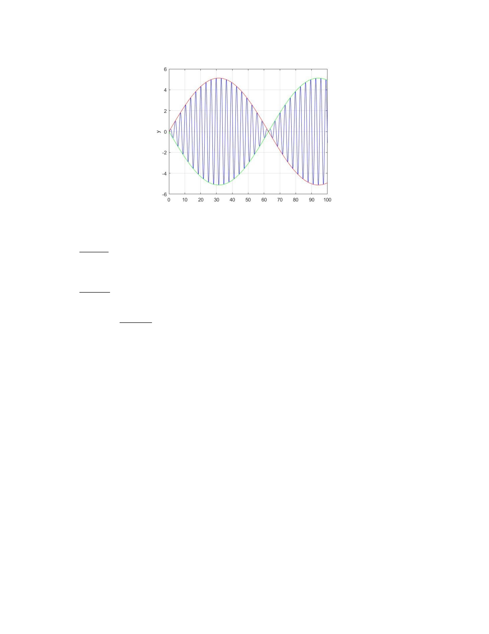
When the value of ω is increased to be closer to ω0, then the length of
the beat seems to increase.
The period of the fast oscillation is
T=4π
(
2+1.9
)
≈3.222
The length of the beat is
T=4π
(
2−1.9
)
≈125.664
Beat Length=125.664
2≈62.8319
This means that the length of the beat doubled while the fast
oscillation period got a little shorter compared to parts b and c.
function LAB06ex1
clc
omega0 = 2; c = 0; omega = 1.6;
param = [omega0,c,omega];
t0 = 0; y0 = 0; v0 = 0; Y0 = [y0;v0]; tf = 100;
options = odeset('AbsTol',1e-10,'relTol',1e-10);
[t,Y] = ode45(@f,[t0,tf],Y0,options,param);
y = Y(:,1); v = Y(:,2);
figure(1)
plot(t,y,'b-'); ylabel('y'); grid on;
C=1/abs(omega0^2-omega^2);
A=2*C*sin((omega0-omega)*t/2);
hold on
plot(t,A,'r-',t,-A,'g-');
%t1 = 25; i = find(t>t1);
%C = (max(Y(i,1))-min(Y(i,1)))/2;
%disp(['computed amplitude of forced oscillation = ' num2str(C)]);
%Ctheory = 1/sqrt((omega0^2-omega^2)^2+(c*omega)^2);
%disp(['theoretical amplitude = ' num2str(Ctheory)]);
%alpha=atan(c*omega/(omega0^2-omega^2));
%yc=y-Ctheory*cos(omega*t-alpha);
%figure(2)
%plot(t,yc,'b-'); grid on; title('complementary solution');
end
%----------------------------------------------------------------
function dYdt = f(t,Y,param)
y = Y(1); v = Y(2);
omega0 = param(1); c = param(2); omega = param(3);
dYdt = [ v ; cos(omega*t)-omega0^2*y-c*v ];
end

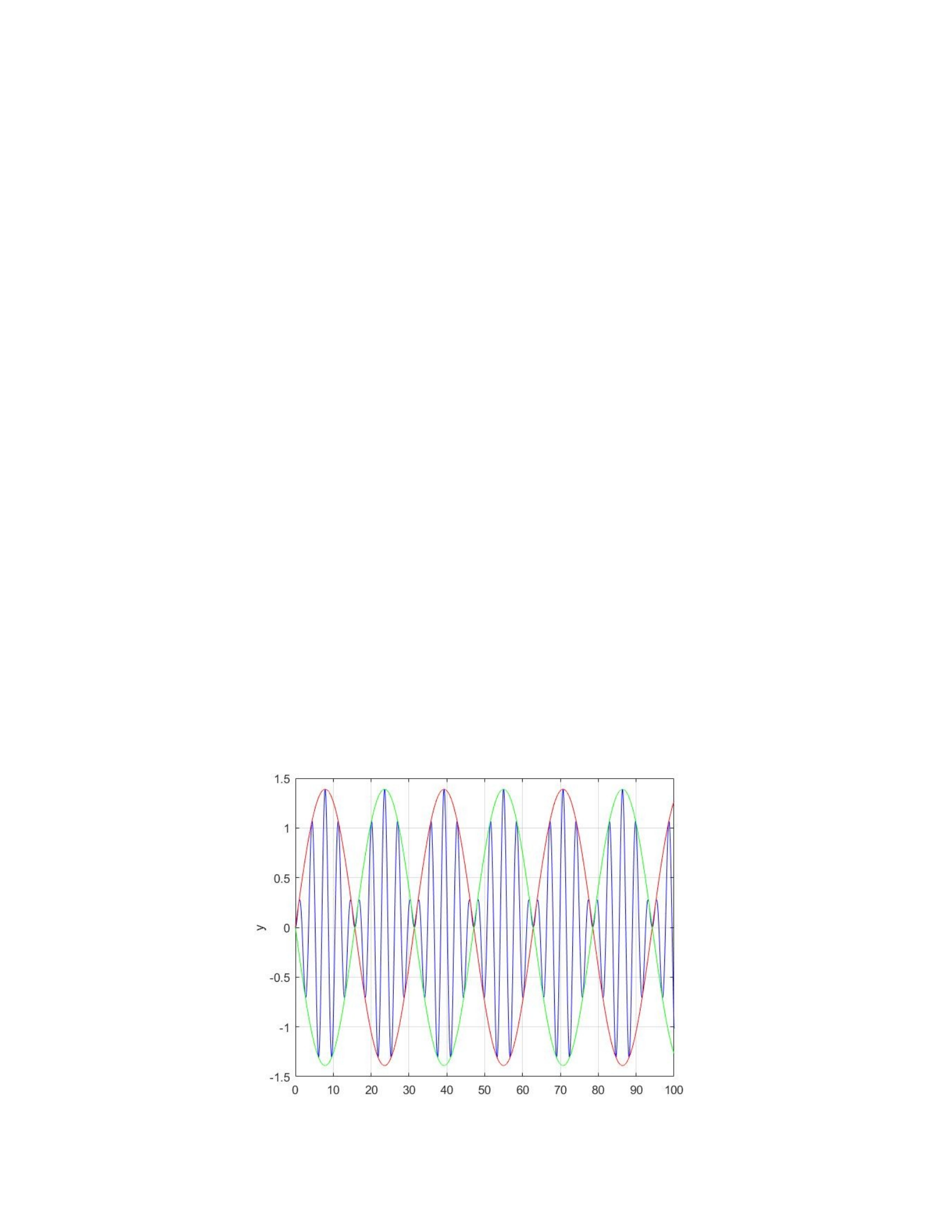
When the value of ω is decreases to be further from ω0, then the
length of the beat seems to decrease.
The period of the fast oscillation is
T=4π
(
2+1.6
)
≈3.49066
The length of the beat is
T=4π
(
2−1.6
)
≈31.4159
Beat Length=31.4159
2≈15.708
This means that the length of the beat halved while the fast
oscillation period got a little longer compared to parts b and c.
(e)
function LAB06ex1
clc
omega0 = 2; c = 0; omega = 0.5;
param = [omega0,c,omega];
t0 = 0; y0 = 0; v0 = 0; Y0 = [y0;v0]; tf = 100;
options = odeset('AbsTol',1e-10,'relTol',1e-10);
[t,Y] = ode45(@f,[t0,tf],Y0,options,param);
y = Y(:,1); v = Y(:,2);
figure(1)
plot(t,y,'b-'); ylabel('y'); grid on;
C=1/abs(omega0^2-omega^2);
A=2*C*sin((omega0-omega)*t/2);
hold on
plot(t,A,'r-',t,-A,'g-');
%t1 = 25; i = find(t>t1);
%C = (max(Y(i,1))-min(Y(i,1)))/2;
%disp(['computed amplitude of forced oscillation = ' num2str(C)]);
%Ctheory = 1/sqrt((omega0^2-omega^2)^2+(c*omega)^2);
%disp(['theoretical amplitude = ' num2str(Ctheory)]);
%alpha=atan(c*omega/(omega0^2-omega^2));
%yc=y-Ctheory*cos(omega*t-alpha);
%figure(2)
%plot(t,yc,'b-'); grid on; title('complementary solution');
end
%----------------------------------------------------------------
function dYdt = f(t,Y,param)
y = Y(1); v = Y(2);
omega0 = param(1); c = param(2); omega = param(3);
dYdt = [ v ; cos(omega*t)-omega0^2*y-c*v ];
end
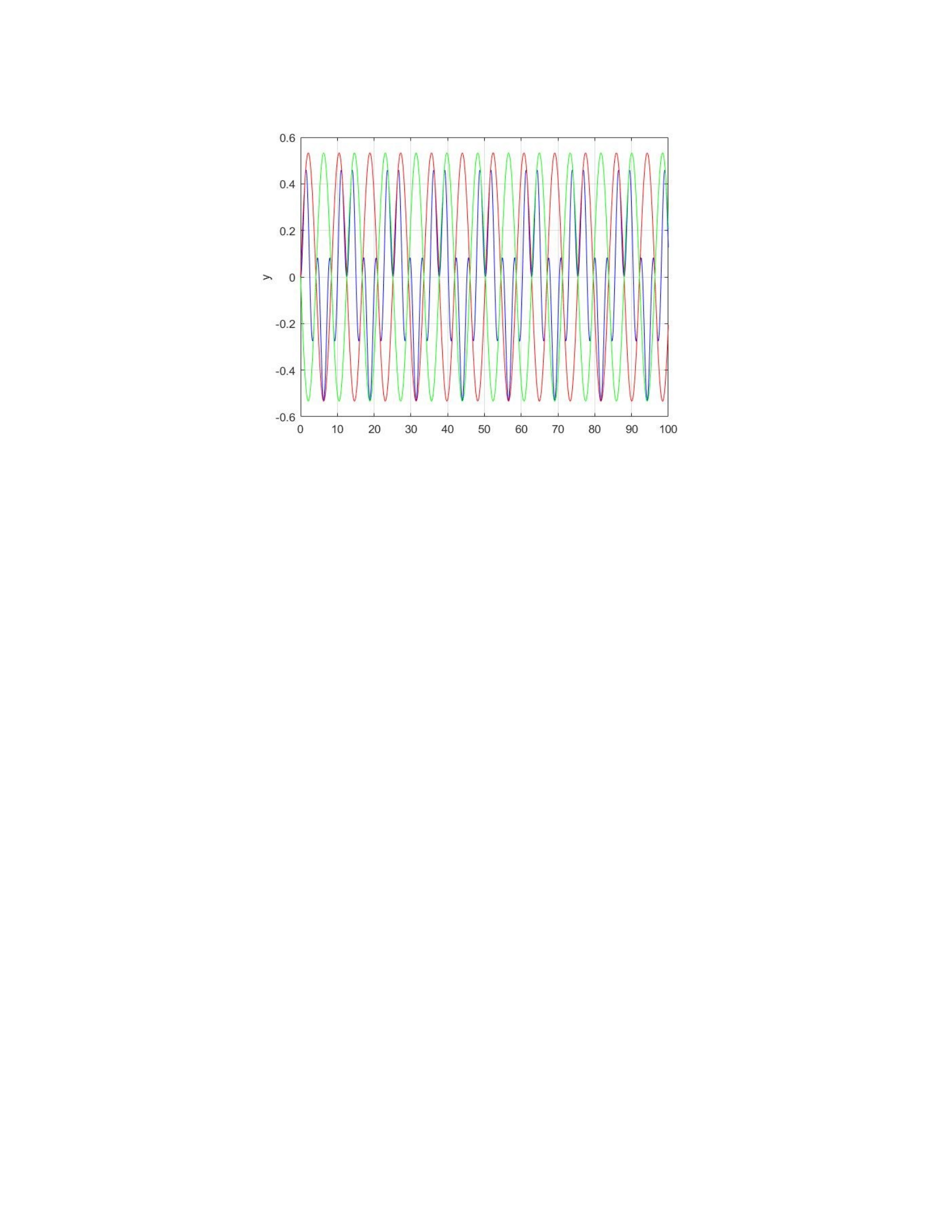
It seems that the beats are still present but they are very short
but he longer oscillations are not lined up with twice the beat length
anymore. This is probably because the value of ω is so far from ω0.

