



Output of the diary file:
% MAT 275 MATLAB Assignment #5
Exercise 1
% Part A of Exercise 1
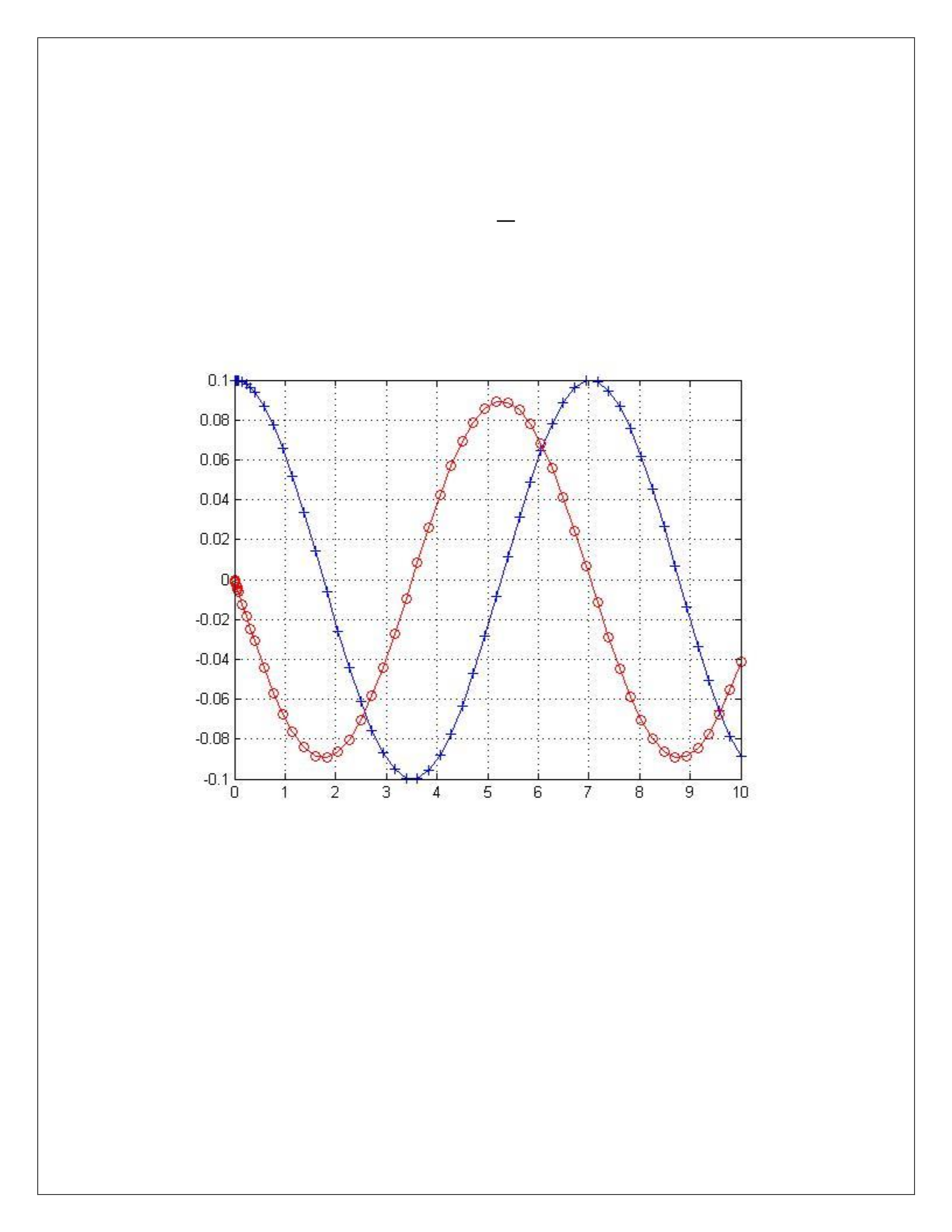
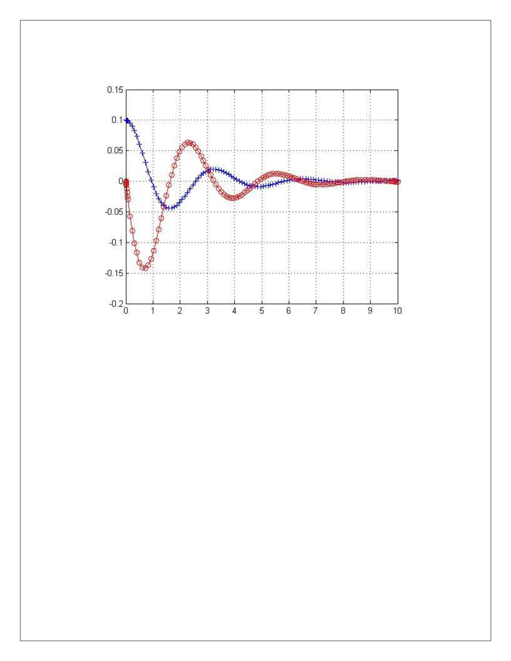
The equation y = y(t) is represented by the curve in “BLUE”.
The equation y = y’(t) is represented by the curve in “RED”.
Since the blue curve starts from a non-zero value at t = 0 suggests that the mass is displaced
initially. Also at t=0 the other curve in red is at the origin. This suggests that the mass is initially
at rest (zero velocity) at t = 0.
% Part B of Exercise 1
Since the curve represents a typical “sinusoidal wave”, the period can be calculated by finding
the time taken in completing one cycle. By looking at the curve for y = y(t), the time period
comes out to be equal to 3.1s. This can be verified by using the following equation –
𝑻 = 𝟐π
ω
With ω = 2 rad/s, the time period T comes out to be equal to π (≈ 3.14).
% Part C of Exercise 1
In an ideal system (i.e. when the damping forces are not present in the system) the mass will
continue to oscillate and will never come to rest. Since the damping forces are ignored there
will be no force which could oppose the motion of the mass.
In a non-ideal system the damping forces (air friction, spring damping factor) will oppose the
motion of the mass and after a while the mass will come to rest.
% Part D of Exercise 1
The initial displacement of the mass is also the maximum displacement/amplitude it can
achieve. As a result the mass continues to oscillate between ±0.1 m (amplitude).
% Part E of Exercise 1
The velocity attains a maximum value when the particle is zero displacement. The maximum
velocity comes out to be approximately equal to 0.99 m/s. Below are the values of “t” where
velocity is maximum -
Instances where velocity is maximum -
i) 2.3904
ii) 3.9415
iii) 5.4479
iv) 7.0329
v) 8.6095
% Part F of Exercise 1
We know that the angular velocity (ω), mass (m) and spring constant (k) satisfy the relation
below -
ω2 = k
m
From the above equation it is evident that the period of oscillation is depends on both k and m.
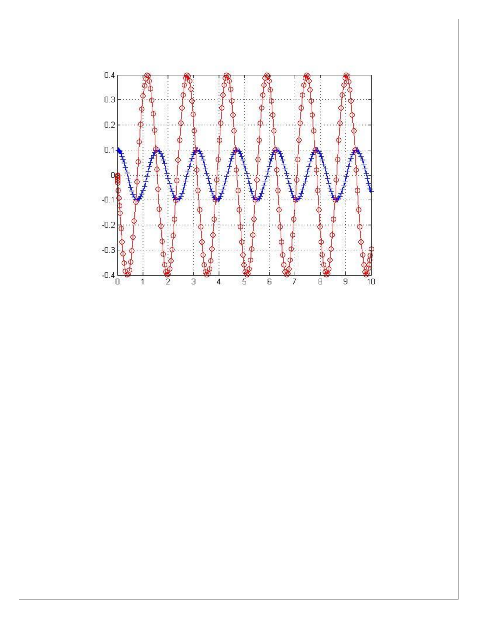
Since T = 2π/ω, therefore as “m” is increased time period also increases {as ω decreases when
m is increased}. The graph below was plotted with k = 4 and m = 5:
When k is increased the Time Period T decreases as ω increases when k is increased. The
following graph illustrates the condition when m = 1 and k = 16:
Exercise 2
% Part A of Exercise 2
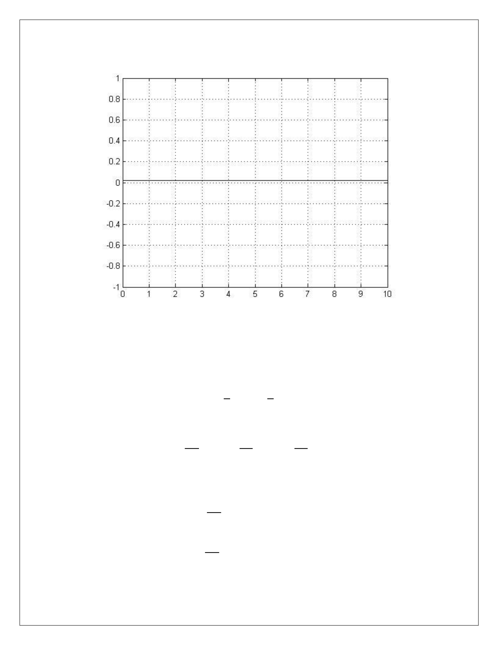
The plot of Energy {E = ½ mv2 + ½ ky2} versus time comes out to be a constant value of around
0.02 units. This confirms the fact that the energy is conserved at all the times as there is no
change in energy. Though there is conversion of energy between kinetic energy of the mass to
spring energy and vice versa. But the entire energy is converted and no energy is lost (clearly an
ideal system). The plot of E vs time is shown below (note y limit was adjusted for a decent plot)
% Part B of Exercise 2
The fact that energy is conserved at all the times should be enough to suggest that the
derivative of energy w.r.t time should be zero. This can be proved mathematically {using the
equation L5.2 and the definition of energy E}
𝐸 = 1
2𝑚𝑣2+1
2𝑘𝑦2
Taking the first derivative -
𝑑𝐸
𝑑𝑡 = 𝑚(𝑣𝑑𝑣
𝑑𝑡)+𝑘(𝑣𝑑𝑦
𝑑𝑡)
Substituting dy/dt as v and dv/dt = g, we get -
𝑑𝐸
𝑑𝑡 = 𝑚𝑣𝑔+𝑘𝑣2
𝑑𝐸
𝑑𝑡 = 𝑣(𝑚𝑔+𝑘𝑣)
From equation L5.2, it is clear that – 𝑚𝑔 = −𝑘𝑣
Therefore,
𝑑𝐸
𝑑𝑡 = 0
This also proves mathematically that the energy is constant with respect to time.
% Part C of Exercise 2
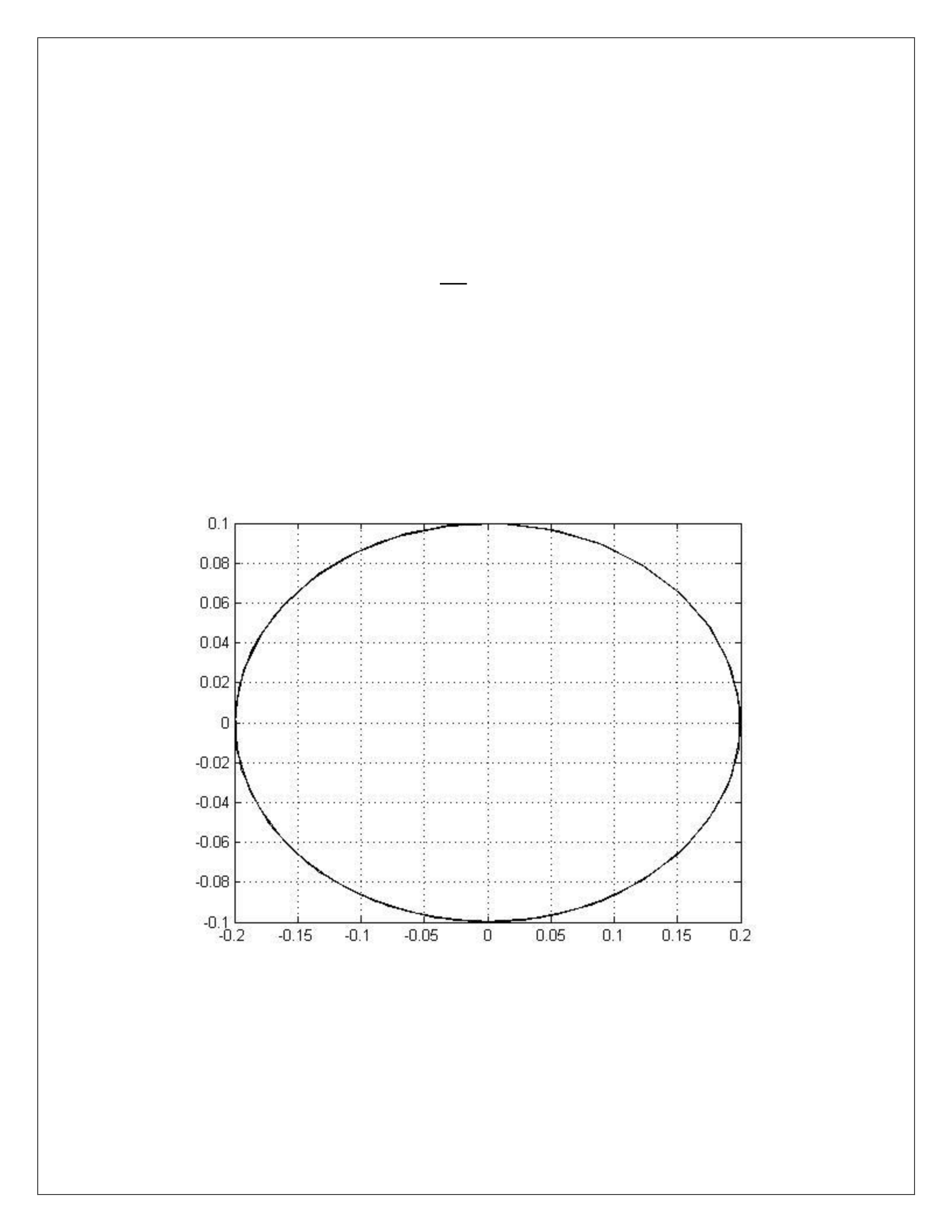
Phase plot between v and y
The curve is not close to the origin at any instant of time “t”. This is true as the all the kinectic
energy is converted into spring energy. Therefore, when the mass is at rest it is at maximum
displacement and the mass is at zero displacement it attains it maximum velocity.
Exercise 3
Figure – v(t) (red) and y(t) (blue)
% Part A of Exercise 3
The Matlab code printed the following output –
>> |y|<0.01 for t>t1 with 3.7807<t1<3.8711
The explanation is given below -
for i=1:length(y)
% Record the maximum displacement at each instant in a matrix
m(i)=max(abs(y(i:end))); % matrix m holds the max displacement
End
% Find the values in m which are less than 0.01
min_m = find(m<0.01); % find will return 1 at those places which
satisfy the equation
% Get the first instant as that would give the minimum t
min_m = min_m(1); % Extracting the first instant from min_m
% Use display for the output
disp(['|y|<0.01 for t>t1 with ' num2str(t(min_m-1)) '<t1<'
num2str(t(min_m))]);

% Part B of Exercise 3
The maximum velocity comes out to be 0.63 m/s at t = 2.26 secs.
% Part C of Exercise 3
c = 2
c = 4
c= 6
c= 8
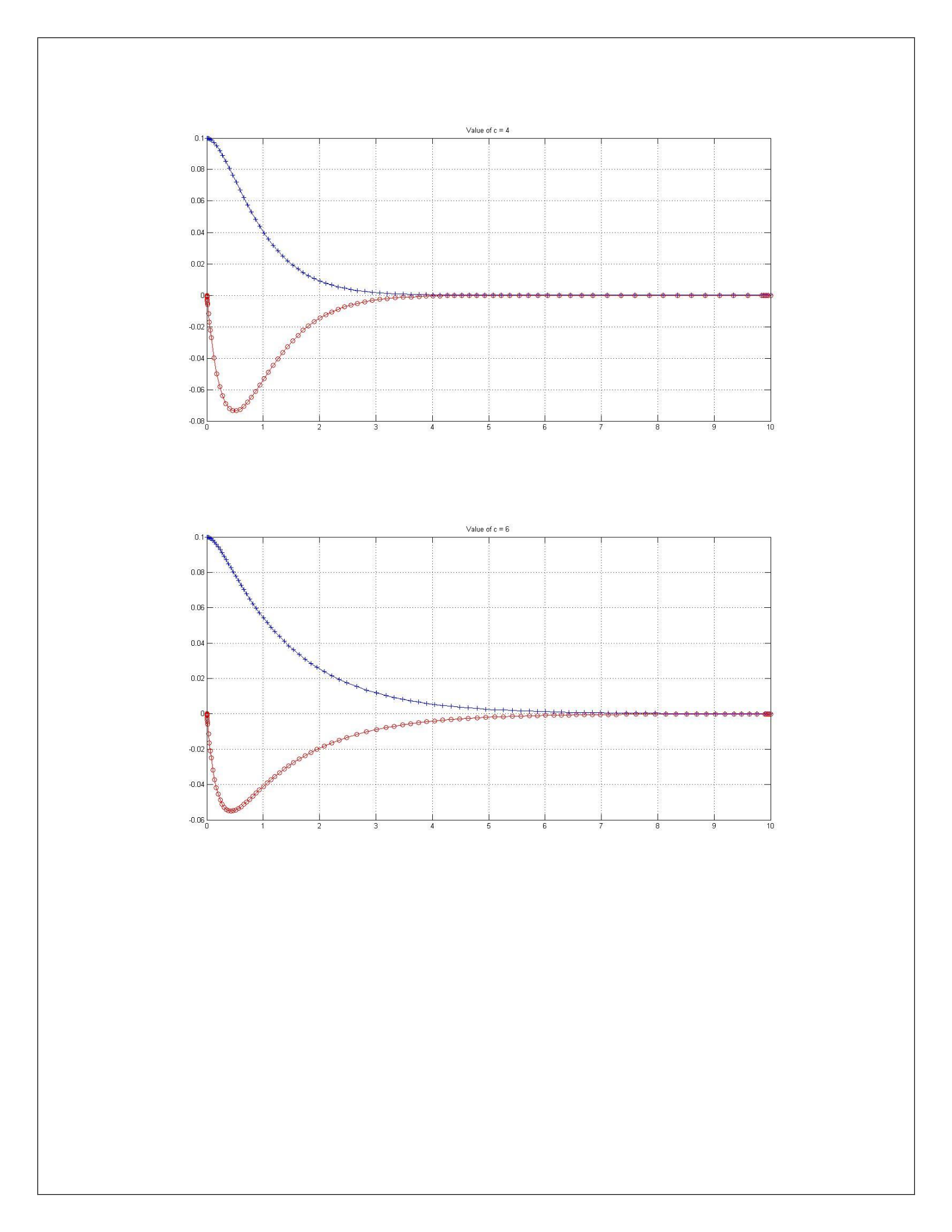
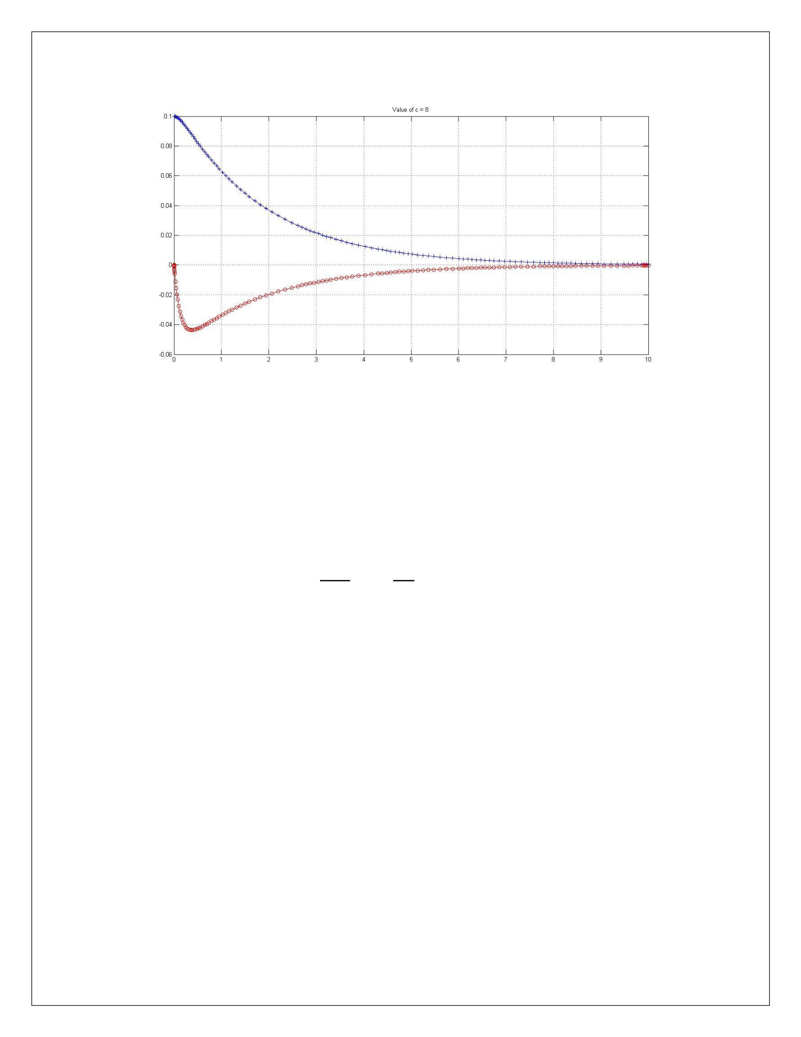
As “c” increases the effect of damping forces also increases. As a result of which the maximum
displacement attained by the mass reduces and it comes to rest after few oscillations.
% Part D of Exercise 3
To calculate minimum “c” at which no oscillations occurs – it is enough to say that this would be
the condition when two equal roots exists {the critical damping case}. The ODE is -
𝑚𝑑2𝑦
𝑑𝑡2+𝑐(𝑑𝑦
𝑑𝑡)+𝑘𝑦 = 0
Initial conditions:
y(0) = yo, y’(0) = vo
The characteristic equation is -
r2 + 2ᶓωr + r2 = 0
By finding the roots
λ1,2 = - ᶓω ± ω (ᶓ2 – 1) ½
If the value of ᶓ is equal to 1, two equal real roots will result.
Therefore, c = 2ᶓω = 4 {ᶓ = 1 and ω = 2} which confirms the value obtained from the graphs
plotted above.
Exercise 4
% Part A of Exercise 4
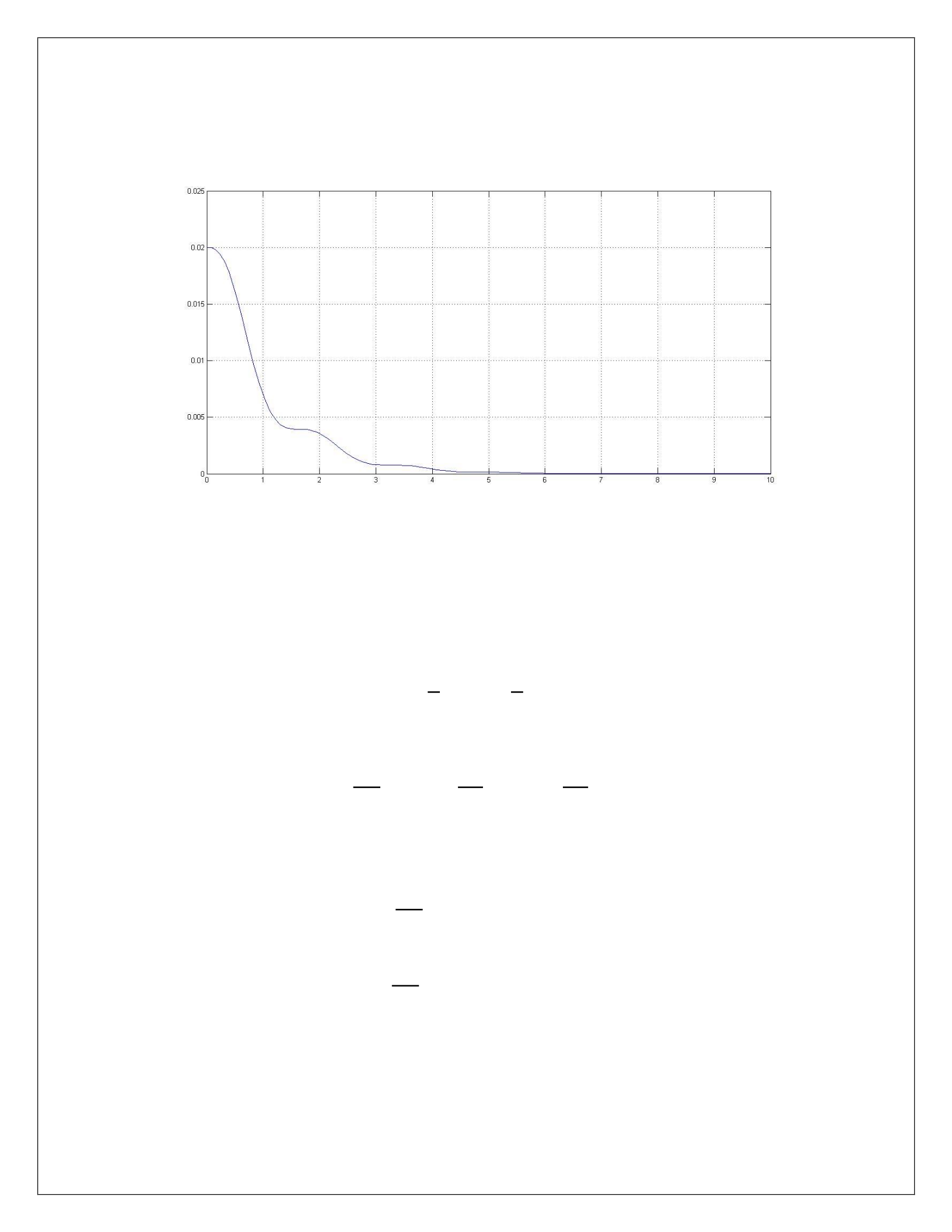
Energy vs Time
The energy is not constant in this case is not conserved.
% Part B of Exercise 4
Mathematically we know that
𝐸 = 1
2𝑚𝑣2+1
2𝑘𝑦2
Taking the first derivative -
𝑑𝐸
𝑑𝑡 = 𝑚(𝑣𝑑𝑣
𝑑𝑡)+𝑘(𝑣𝑑𝑦
𝑑𝑡)
Substituting dy/dt as v and dv/dt = g, we get -
𝑑𝐸
𝑑𝑡 = 𝑚𝑣𝑔+𝑘𝑣2
𝑑𝐸
𝑑𝑡 = 𝑣(𝑚𝑔+𝑘𝑣)
From equation L5.4, it is clear that – 𝑚𝑔+𝑘𝑣 = −𝑐𝑣
Therefore,
𝑑𝐸
𝑑𝑡 = −𝑐𝑣
Thus when c>0, dE/dt < 0 and vice versa.
% Part C of Exercise 4
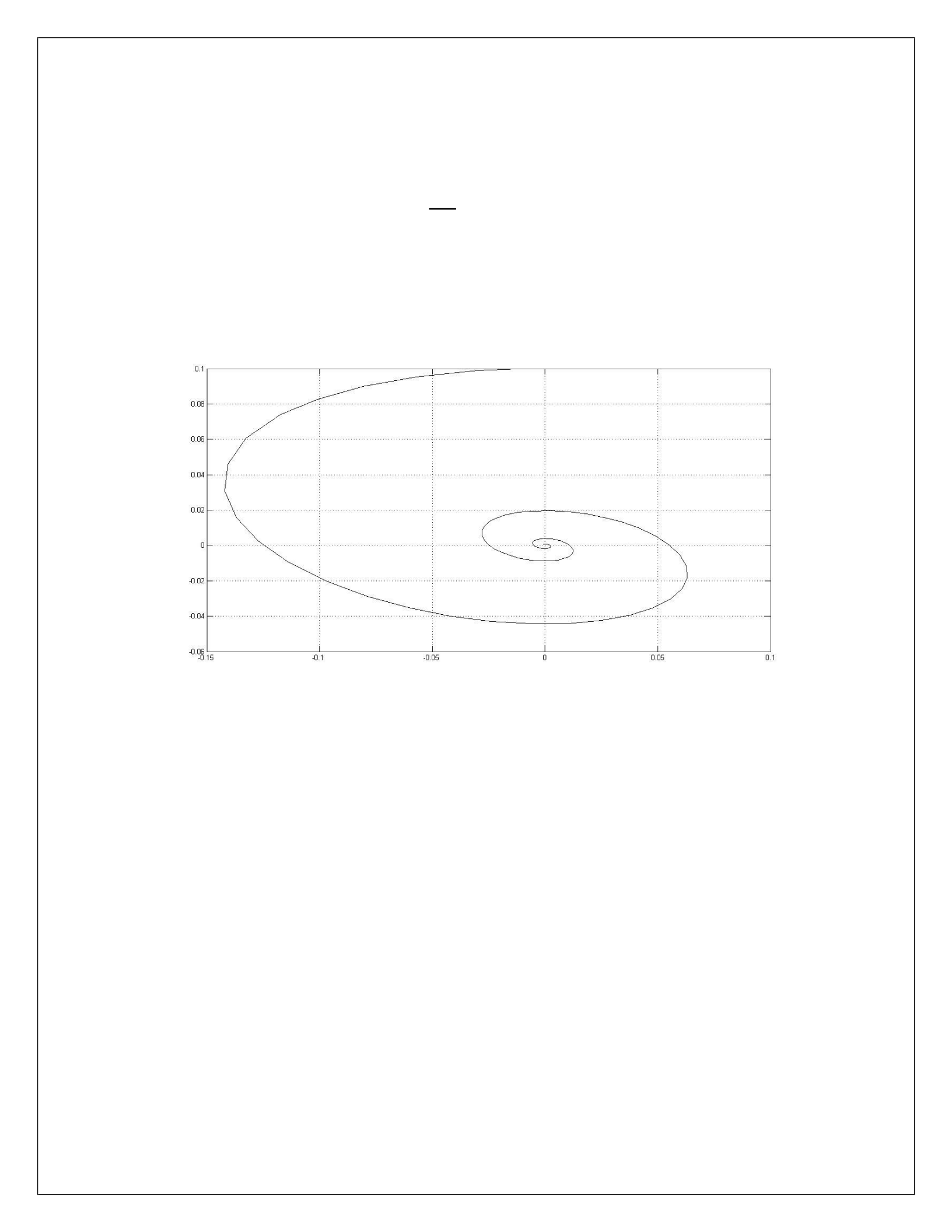
Figure – v vs y
The plot gets neared to origin. Due to damping forces, the energy is not conserved. Due to
which there is some loss in the energy as in the entire kinectic/spring energy does not get
converted to spring/kinetic energy. Due to this mass finally stops oscillating which suggests that
it gets nearer to the origin.

