Mat 275 MATLAB LAB #6
Name: Brandon Grebe
Lab Day and Time: Wednesday
10:30
Instructor: Chowell Puente
Exercise #1
Part A
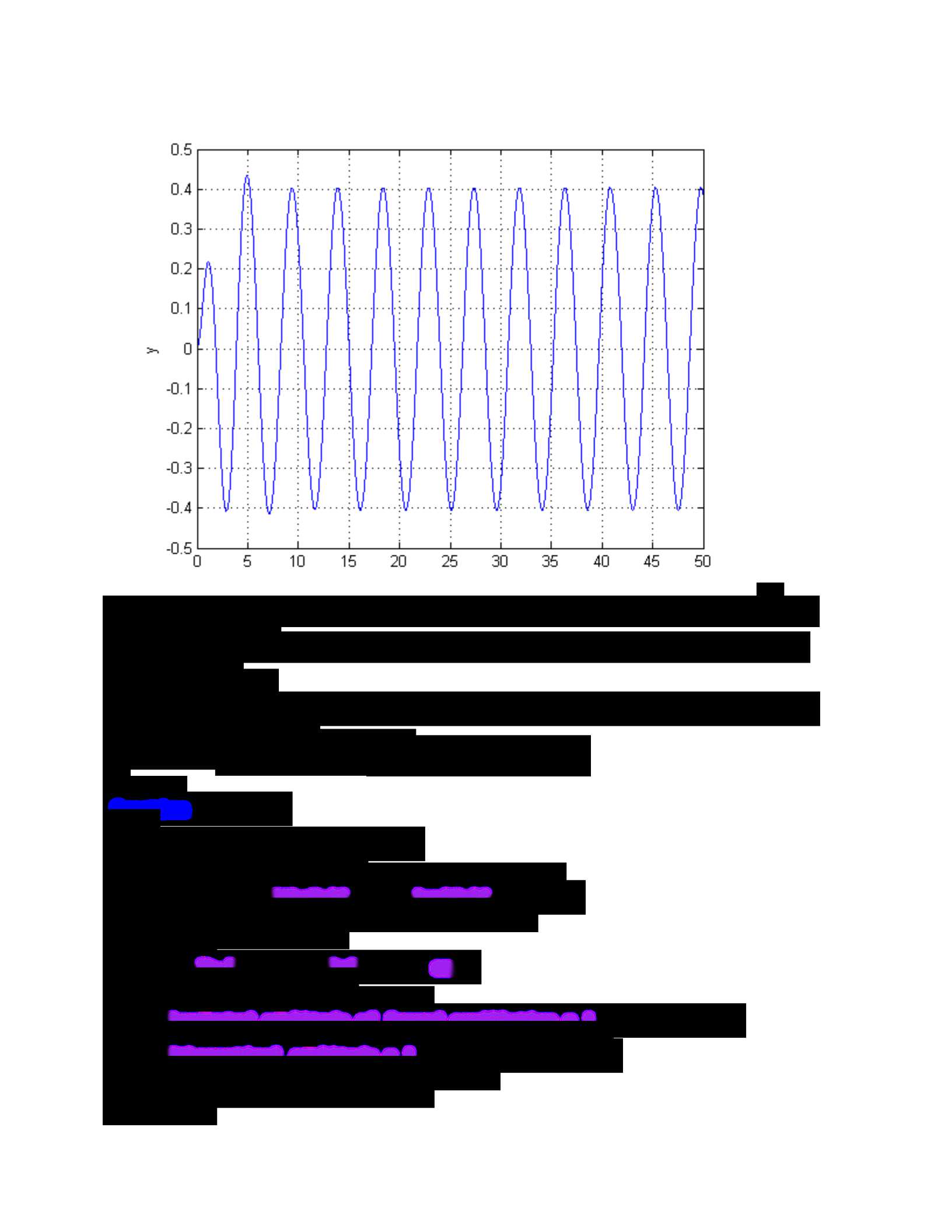
By running the given function file we can see the graph of the solution as
well as find the period of this forced oscillation.
function LAB06ex1
clc
omega0 = 2; c = 1; omega = 1.4;
param = [omega0,c,omega];
t0 = 0; y0 = 0; v0 = 0; Y0 = [y0;v0]; tf = 50;
options = odeset( ,1e-10,'AbsTol' 'relTol',1e-10);
[t,Y] = ode45(@f,[t0,tf],Y0,options,param);
y = Y(:,1); v = Y(:,2);
figure(1)
plot(t,y,'b-'); ylabel( ); grid ;'y' on
t1 = 25; i = find(t>t1);
C = (max(Y(i,1))-min(Y(i,1)))/2;
disp([ num2str(C)]);'computed amplitude of forced oscillation = '
Ctheory = 1/sqrt((omega0^2-omega^2)^2+(c*omega)^2);
disp([ num2str(Ctheory)]);'theoretical amplitude = '
%----------------------------------------------------------------
function dYdt = f(t,Y,param)
y = Y(1); v = Y(2);
omega0 = param(1); c = param(2); omega = param(3);
dYdt = [ v ; cos(omega*t)-omega0^2*y-c*v ];