


MAT 275 LAB 6
Fenil Patel
1215196606
1.
a)
Time period (T) = 2*pi/omega
= 2*3.14/4.6
= 1.37 s
The numerical value of alpha is 1.9286 rad.
b) clear all; %this deletes all variables
omega0=4;c=3;omega=4.6;
param = [omega0,c,omega];
t0=0;y0=0;v0=0;Y0=[y0;v0];tf=30;
options = odeset('AbsTol',1e-10,'relTol',1e-10);
[t,Y] = ode45(@f,[t0,tf],Y0,options ,param);
y = Y(:,1); v = Y(:,2);
figure (1)
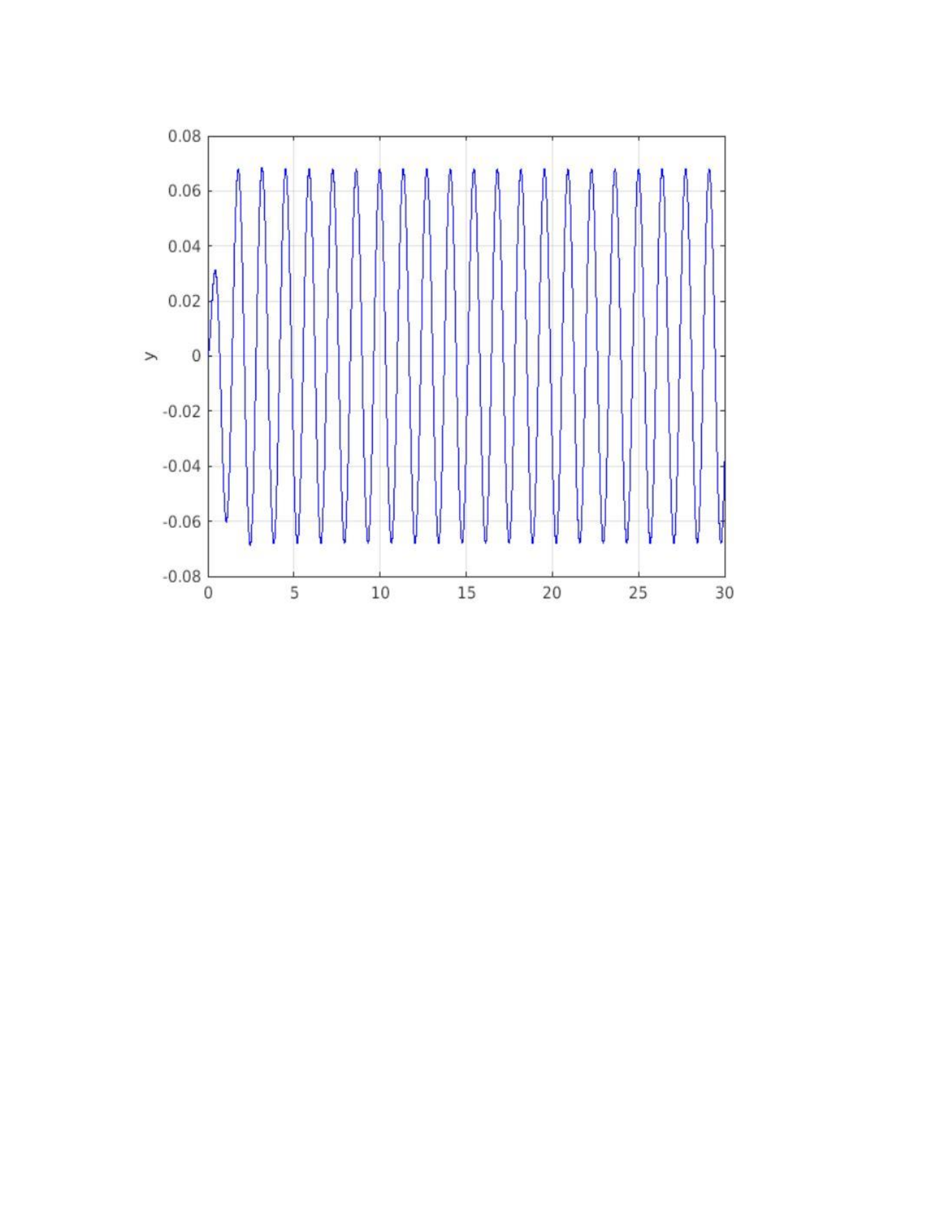
plot(t,y,'b-'); ylabel('y'); grid on;
t1 = 9; i = find(t>t1);
C = (max(Y(i,1))-min(Y(i,1)))/2;
disp(['computed amplitude of forced oscillation = ', num2str(C)]);
Ctheory = 1/sqrt((omega0^2-omega^2)^2+(c*omega)^2);
disp(['theoretical amplitude = ', num2str(Ctheory)]);
alpha = pi + atan(c*omega/(omega0^2-omega^2));
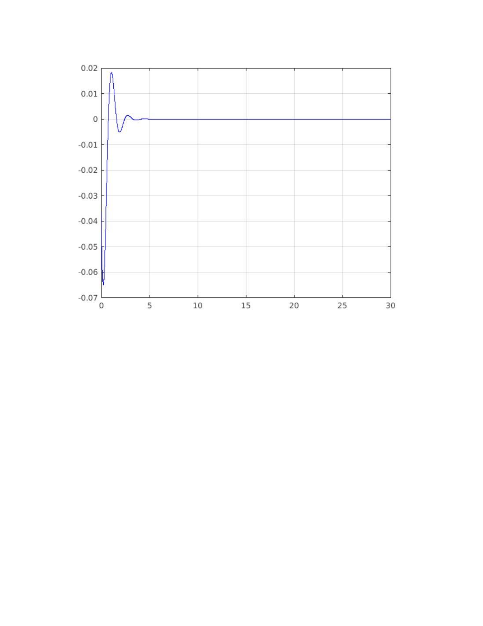
yc = y - Ctheory*cos(omega*t-alpha);
figure (2)
plot(t,yc,'b-');
grid on;
%----------------------------------------------------------------
function dYdt = f(t,Y,param)
y=Y(1);v=Y(2);
omega0 = param (1); c = param (2); omega = param (3);
dYdt = [ v ; cos(omega*t)-omega0^2*y-c*v ];
end
computed amplitude of forced oscillation = 0.067874
theoretical amplitude = 0.067874
0.08
0.06
0.04
0.02
0.02
-0.04
-0.06
-0.08
10 15
20
25
30
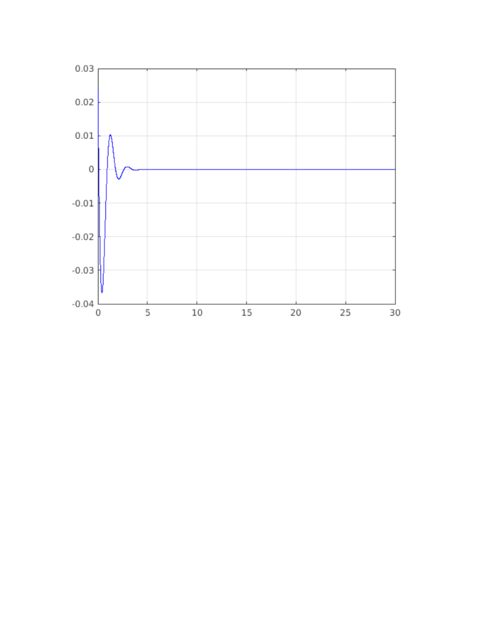
Yes the graph looks like an exponentially decreasing oscillation, as the value of function decreases to
zero at t = infinity.
2.
a)
clear all; %this deletes all variables
omega0 = 4; c = 3;
OMEGA =2:0.01:5;
C = zeros(size(OMEGA));
Ctheory = zeros(size(OMEGA));
t0 = 0; y0 = 0; v0 = 0; Y0 = [y0;v0]; tf =30; t1 = 9;
for k = 1:length(OMEGA)
omega = OMEGA(k);
param = [omega0,c,omega];
[t,Y] = ode45(@f,[t0,tf],Y0,[],param);
i = find(t>t1);
C(k) = (max(Y(i,1))-min(Y(i,1)))/2;
Ctheory(k) = 1/sqrt((omega0^2-omega^2)^2+(c*omega)^2);
end
figure(2)
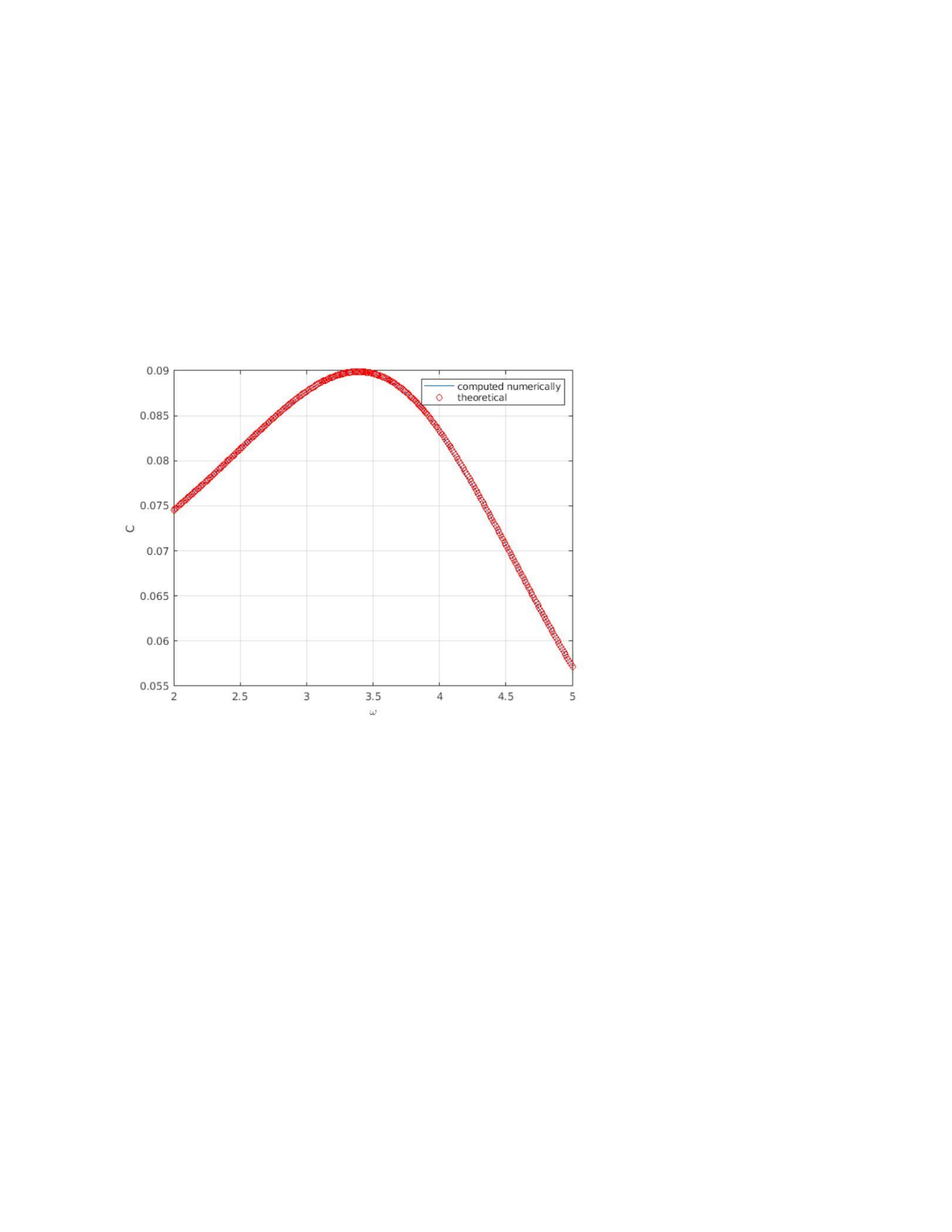
plot(OMEGA,C,OMEGA,Ctheory,'ro'); grid on; % FILL-IN to plot C and Ctheory as a
function of OMEGA
xlabel('\omega'); ylabel('C');
legend('computed numerically','theoretical')
%---------------------------------------------------------
function dYdt = f(t,Y,param)
y = Y(1); v = Y(2);
omega0 = param(1); c = param(2); omega = param(3);
dYdt = [ v ; cos(omega*t)-omega0^2*y-c*v ];
end
b) The maximum value of C is 0.09 at w = 3.39.
c) C = 1/sqrt((16-w^2)^2+9w^2)
C’ = 0 = - w(2w^2-23)/((16-w^2)^2+9w^2)
Thus,
2w^2- 23 = 0
w = 3.39
Thus, C = 0.09.
o1
0.08
0.06
0.04
0.02
-0.02
-0.04
-0.06
-0.08
-0.1
10 15
20
25 30
d)
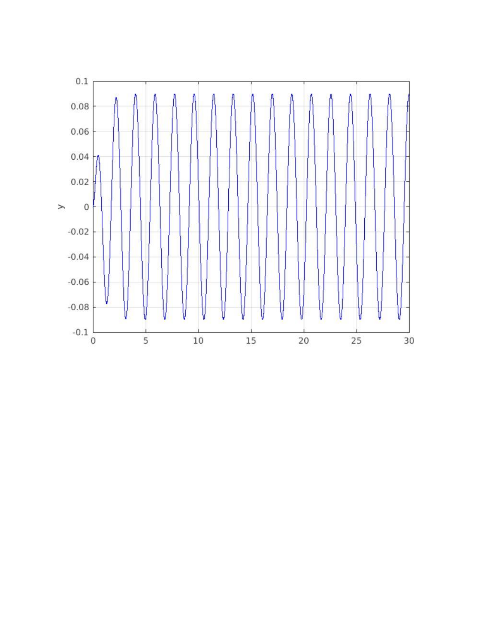
computed amplitude of forced oscillation = 0.089893
theoretical amplitude = 0.089893
The amplitude of forced oscillation is greater than the previous plots.
e) The value of C is not affected by the initial conditions and thus the plot was
not changed when the initial conditions were changed.
3.
a)
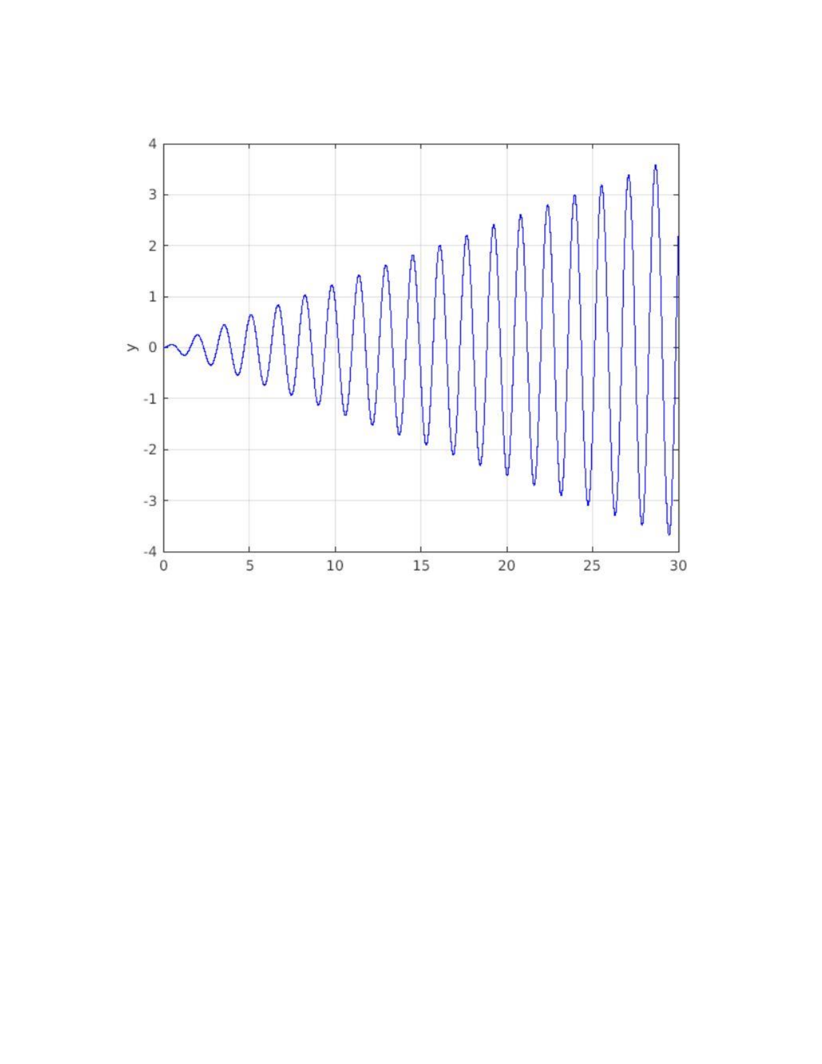
The amplitude increases as the value of w reaches the value of w0 as it is
inversely proportional to w0^2-w^2. The maximal value of C is achieved at w = w0
= 4.
b)
The amplitude of solution keep increasing with time.
4.
a)
clear all; %this deletes all variables
omega0=4;c=0;omega=4.1;
param = [omega0,c,omega];
t0=0;y0=0;v0=0;Y0=[y0;v0];tf=80;
options = odeset('AbsTol',1e-10,'relTol',1e-10);
[t,Y] = ode45(@f,[t0,tf],Y0,options ,param);
y = Y(:,1); v = Y(:,2);
t1 = 9; i = find(t>t1);
C = (max(Y(i,1))-min(Y(i,1)))/2;
disp(['computed amplitude of forced oscillation = ', num2str(C)]);
Ctheory = 1/sqrt((omega0^2-omega^2)^2+(c*omega)^2);
disp(['theoretical amplitude = ', num2str(Ctheory)]);
C = 1/abs(omega0^2-omega^2);
A = 2*C*sin((omega0-omega)*t/2);
figure (1)
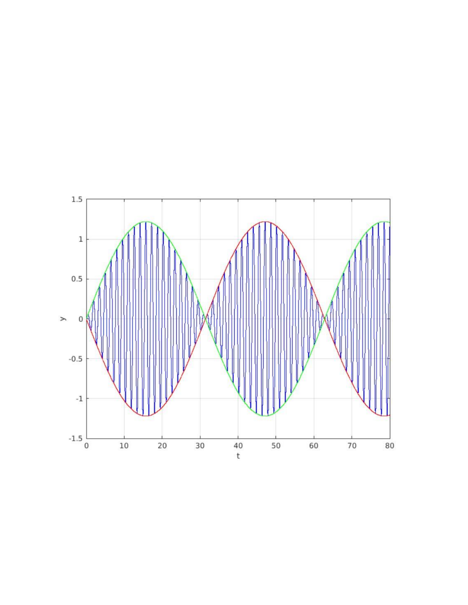
plot(t,y,'b-'); xlabel('t'); ylabel('y'); grid on;
hold on
plot(t,A,'r-',t,-A,'g-');
grid on
%----------------------------------------------------------------
function dYdt = f(t,Y,param)
y=Y(1);v=Y(2);
omega0 = param (1); c = param (2); omega = param (3);
dYdt = [ v ; cos(omega*t)-omega0^2*y-c*v ];
end
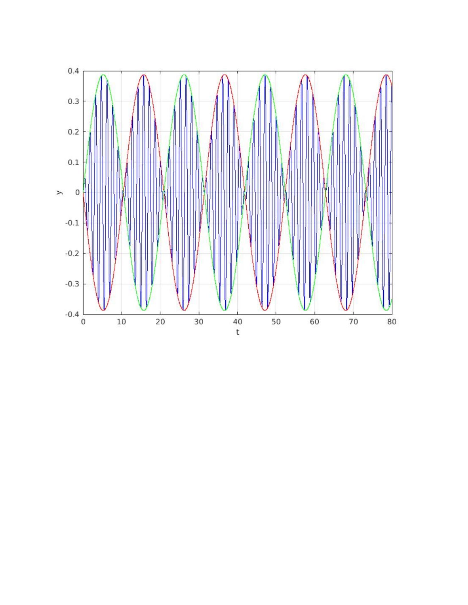
b) 4*pi/(w0 +w) = 1.53s
c) 31.4 s
d)
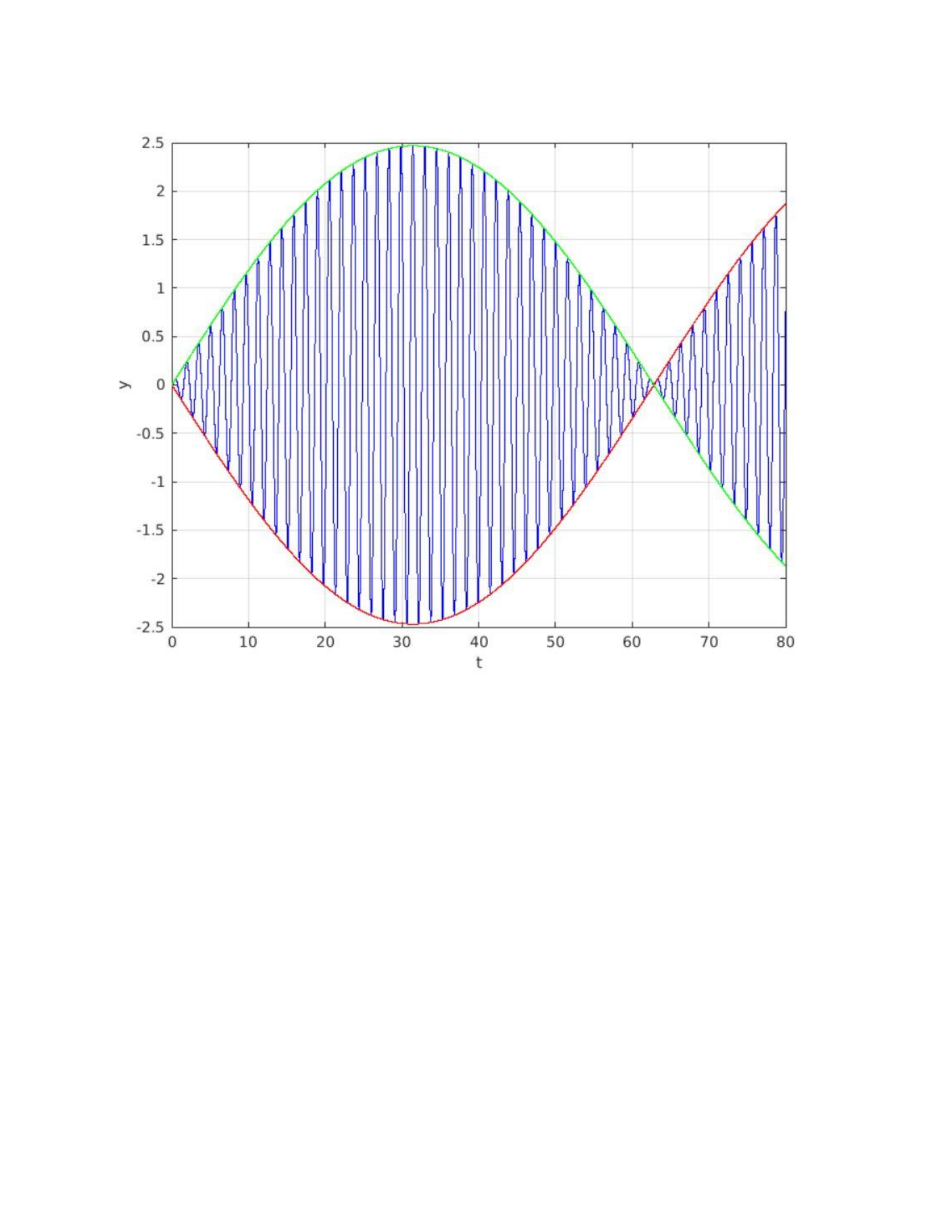
W0 =4 and w = 4.1
Period of forced oscillation = 1.55s
Length of beats = 62.84s
W0 =4 and w = 4.6
Period of forced oscillation = 1.46s
Length of beats = 10.47s
e) The beats phenomenon will not be present at w= 2 because for a beat to occur the value of w should
be close to the value of w0 =4.

