


MAT 275 Lab #5
clear all
close all
Exercise 1
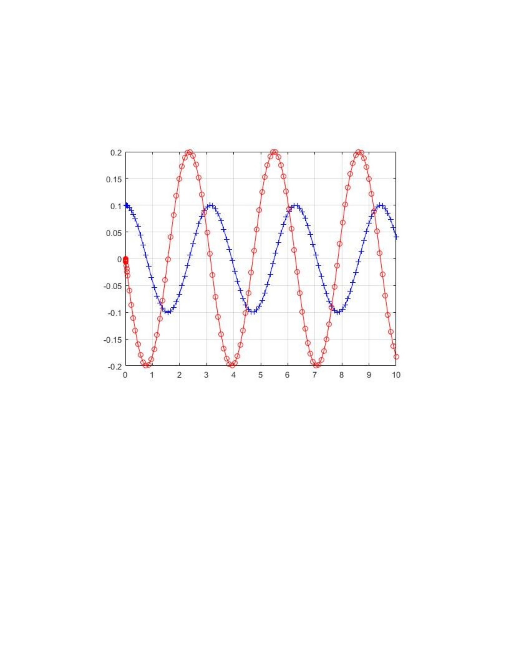
Original Graph showing y and v vs t
a)
The graph L5a, is graphing 'y' and 'v' against t, where v=y'
using the initial conditions it is easy to determine that the blue graph is
a positive cosine curve, and the red graph is a negative sine curve.
Respectively, the derivative of cosine is negative sine, so the positive
cosine curve (blue) is y and the negative sine (red) is v or y'.
b)
By reading the graph, the period seems to be about 3 for both curves.
Looking at it analytically, the period is actually pi. For an unmodified
cosine or sine curve, the period is 2pi. In this case it is given that
omega(0)
is 2. To determine the period in a modified cosine curve, the original
period is divided by the coefficient inside the cosine. Meaning 2pi gets
divided by 2, and the period comes out to be 3.14 (pi)
c)The graph appears to show that the oscillating object has no damper on
it, so it will remain perpetually in motion. Meaning is will not come to
rest.
d)The amplitude is 0.1. It is determined from the graph by reading the
peaks and troughs and how far they extend from equilibrium point.
e)
The maximum velocity that the mass attains is at 3/4*pi. Each
corresponding t value with that same maximum velocity can be found using
3/4*pi+n*pi where n=any integer
f)
the spring constant k effects the potential energy that can be in the
system. So the stiffer the spring, the higher the potential energy. The
mass comes into play once the oscillation has begun, because potential
energy has been converted to kinetic energy. With the same k but differing
masses, the smaller mass will result in a higher velocity while the
larger mass will require more energy to move and will have a lower
velocity.
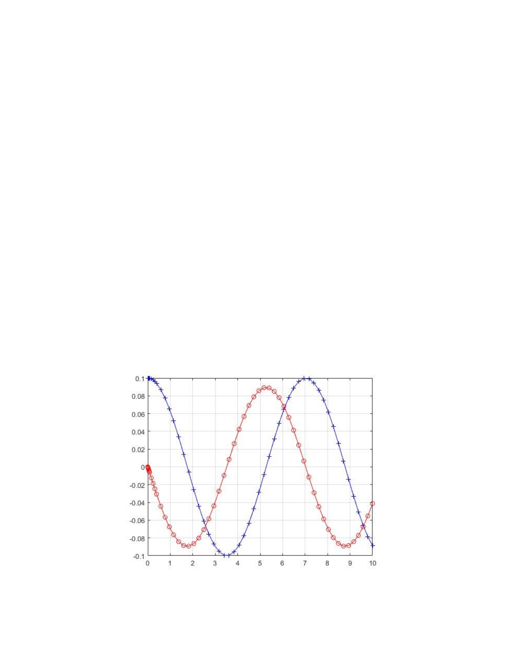
In the graph that shows that the mass is 5 and the spring constant is 4
(this is the same as the original graph, but the mass has increased from 1
to 5), the velocity is significantly decreased as shown in the amplitude
of the y' (red) curve. In the graph where mass is 1 and spring constant is
16, the velocity is significantly larger than when the spring constant is
high and the mass is small.
Analytically, it is given that omega(0)^2=k/m. So every time the spring
constant is multiplied by 4, the period is doubled. This is shown in
comparing the original graph where m=1 and k=4 and in the second modified
graph which included m=1 and k=16. The k has increased by a factor of 4 to
16, meaning the period has doubled from pi, to 2*pi.
First modified graph showing m=5 and k=4
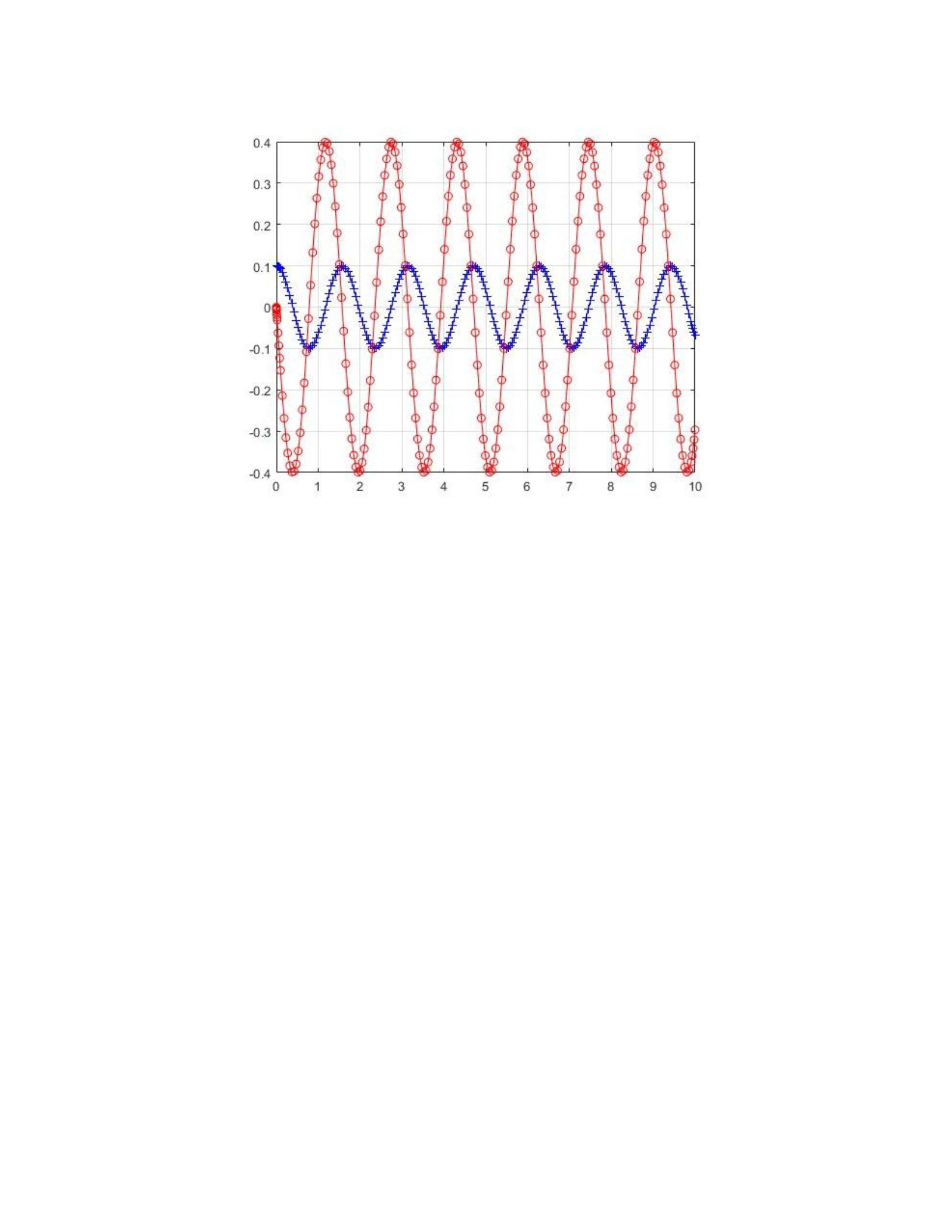
Second modified graph showing m=1 and k=16
Exercise 2
a)
type('LAB05ex1')
function LAB05ex1
m = input('type your desired mass value '); % mass [kg]
k = input('type your desired spring constant ');% spring constant [N/m]
omega0=sqrt(k/m);
y0=0.1; v0=0; % initial conditions
[t,Y]=ode45(@f,[0,10],[y0,v0],[],omega0); % solve for 0<t<10
y=Y(:,1); v=Y(:,2); % retrieve y, v from Y
figure(1); plot(t,y,'b+-',t,v,'ro-'); % time series for y and v
grid on;
K=(1/2)*m*v.^2; %Kinetic Energy
P=(1/2)*k*y.^2; %Potential Energy
E=K+P; %Total energy
figure(2);plot(t,E,'r+-')%Plots energy over time, should be a horizontal
line.
grid on;
figure(3);plot(K,P,'yo-') %Energy by energy, shows that it is conserved
grid on;
figure(4);plot(v,y,'-g*') %Phase plot that shows velocity related to
positions
grid on;
end
%% ------------------------------------------------------
function dYdt= f(t,Y,omega0)
y = Y(1); v= Y(2);
dYdt = [v; -omega0^2*y];
end
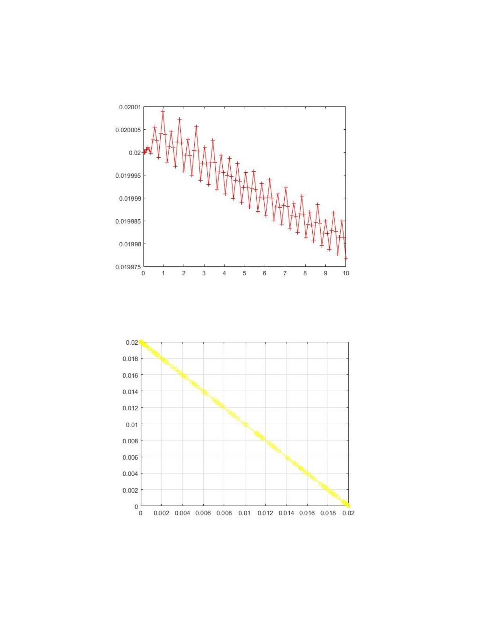
In this graph (figure 2 shown below), the total energy of the system is equal
to Kinetic + Potential. So in a system where energy is conserved, the total
energy will not change over time. This graph does not show a straight line,
but the change in energy is so miniscule it can be ignored.
Figure 2: Total Energy vs time
The command 'ylim' did not work in my function, so I chose to plot Kinetic vs
Potential Energy(shown in figure 3 below) that shows that energy is conserved
and must be .02 at all time when adding P and K
Figure 3: Kinetic vs Potential Energy
b)
The derivative of a constant function is equal to 0. Because the energy in
the system doesn't change; it is a constant function. So, when it is
derived the result will be 0.
c)
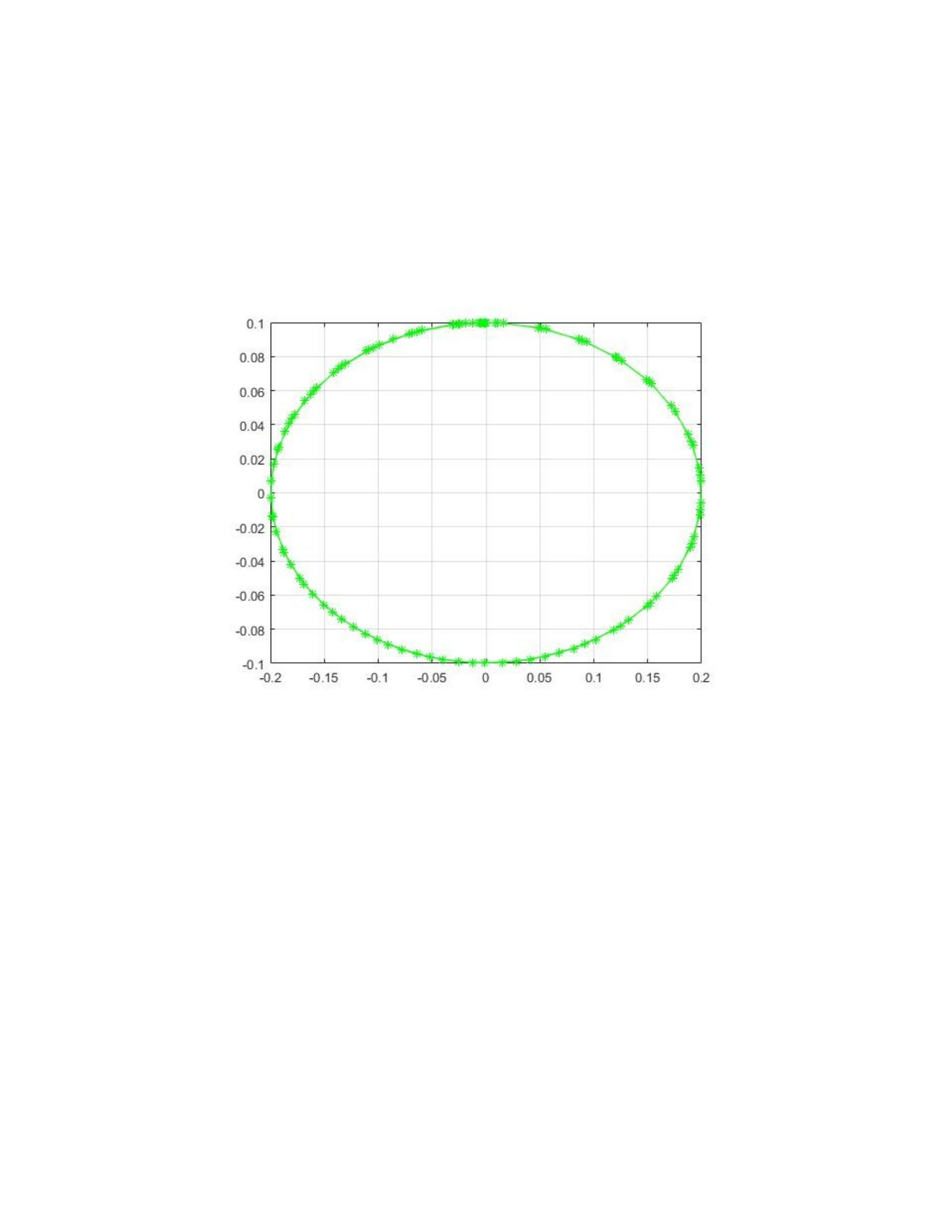
The phase plot is shown in figure 4 (green stars). It shows that the curve
never gets close to the origin because energy is conserved, meaning that
a certain position of the mass will always result in the same velocity at
that point.
Figure 4: Phase Plot showing v vs y
Exercise 3
type('Attempt2') %This file has been renamed from LAB05ex1a
function LAB05ex1a
m = 1; % mass [kg]
k = 4; % spring constant [N/m]
c = input('type desired friction coefficient'); % friction coefficient
[Ns/m]
omega0 = sqrt(k/m); p = c/(2*m);
y0 = 0.1; v0 = 0; % initial conditions
[t,Y] = ode45(@f,[0,10],[y0,v0],[],omega0,p); % solve for 0<t<10
y = Y(:,1); v = Y(:,2); % retrieve y, v from Y
figure(1); plot(t,y,'b+-',t,v,'ro-'); % time series for y and v
grid on;
K=(1/2)*m*v.^2; %Kinetic Energy
P=(1/2)*k*y.^2; %Potential Energy
E=K+P; %Total energy
figure(2);plot(t,E,'r+-') %Plots energy over time, should be a
horizontal line.
grid on;
figure(3);plot(K,P,'yo-') %Energy by energy, shows that it is conserved
grid on;
figure(4);plot(v,y,'-g*') %Phase plot that shows velocity related to
positions
grid on;
for i=1:length(y)
m(i)=max(abs(y(i:end)));
end
i = find(m<0.01); i = i(1);
disp(['|y|<0.01 for t>t1 with ' num2str(t(i-1)) '<t1<' num2str(t(i))])
figure(4);plot(v,y,'-g*')
end
%-------------------------------------------
function dYdt = f(t,Y,omega0,p)
y = Y(1); v = Y(2);
dYdt = [ v ; -omega0^2*y-2*p*v ]; % fill-in dv/dt
end
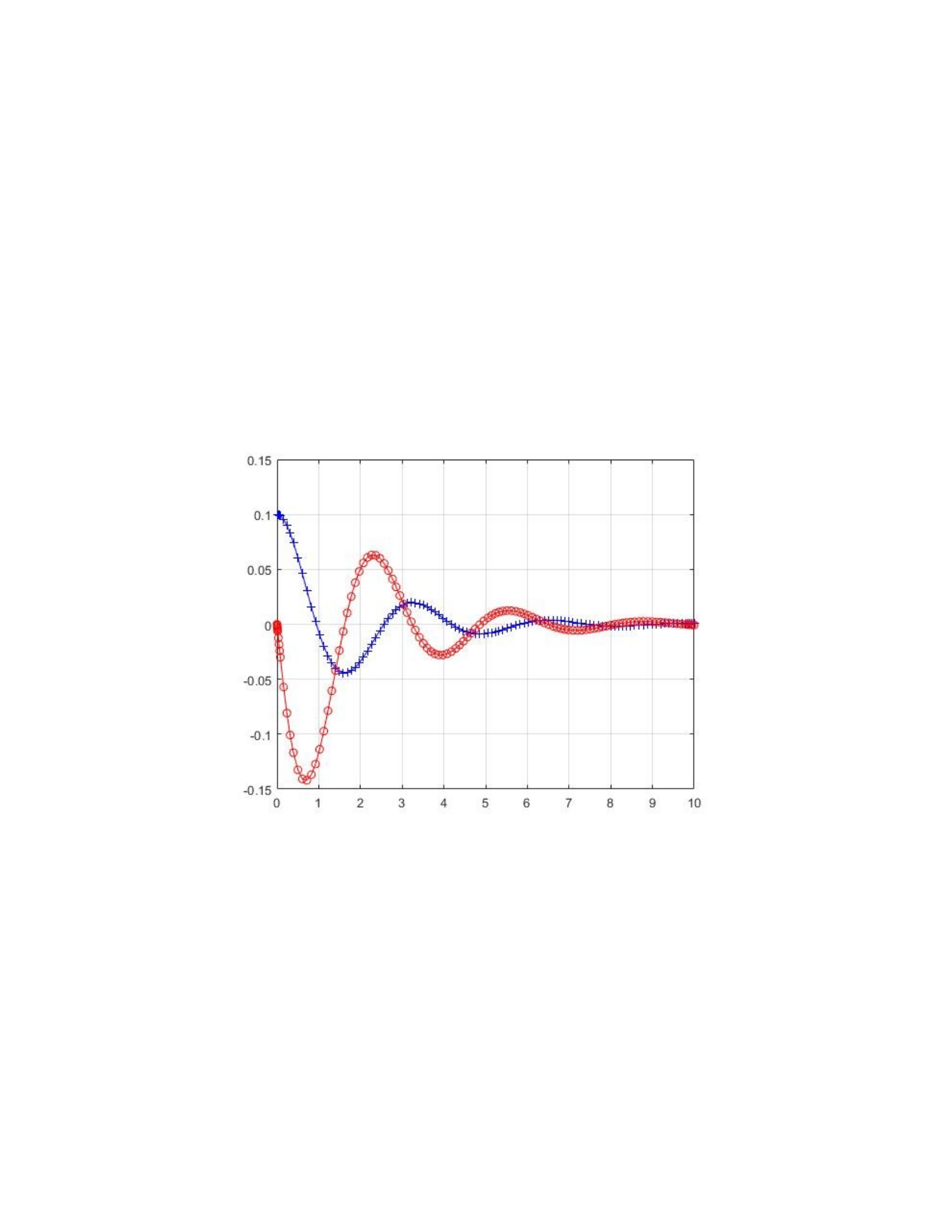
Original Graph in Dampened System
a)
The minimum value for t1=3.780
Shown when the command below is run(this command can be found in file
‘Attempt2’):
i = find(m<0.01); i = i(1);
disp(['|y|<0.01 for t>t1 with ' num2str(t(i-1)) '<t1<' num2str(t(i))])
figure(4);plot(v,y,'-g*')
b)
The maximum value for the y' velocity (red) curve, is about .142. It is
negative, however, the negative only refers to the direction the mass is
moving, so either way the maximum velocity is the first extrema that the
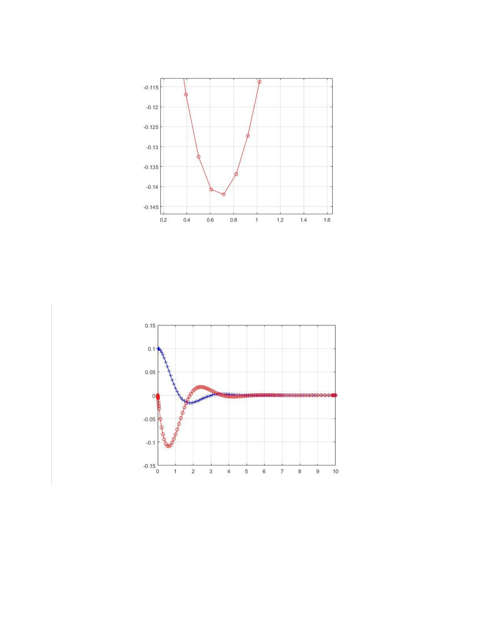
mass reaches.
Maximum Value of Velocity for Dampened System
c)
The size of the coefficient of friction determines how long the mass will
oscillate before it comes to rest (it reaches an arbitrarily small
distance from the equilibrium). The larger the coefficient of friction,
the sooner the mass will come to rest.
C=2

C=4
C=6
C=8
d)
Analyzing the graphs where c=3 and c=4, it is shown that the critical
value where c is strong enough that the mass doesn't oscillate lays
between those numbers. When analyzing c=3.5, it is possible to see that
the oscillation is miniscule and has virtually come to rest.
Exercise 4
*All changes in order to determine values can be
found in the file ‘Attempt2’.
a)
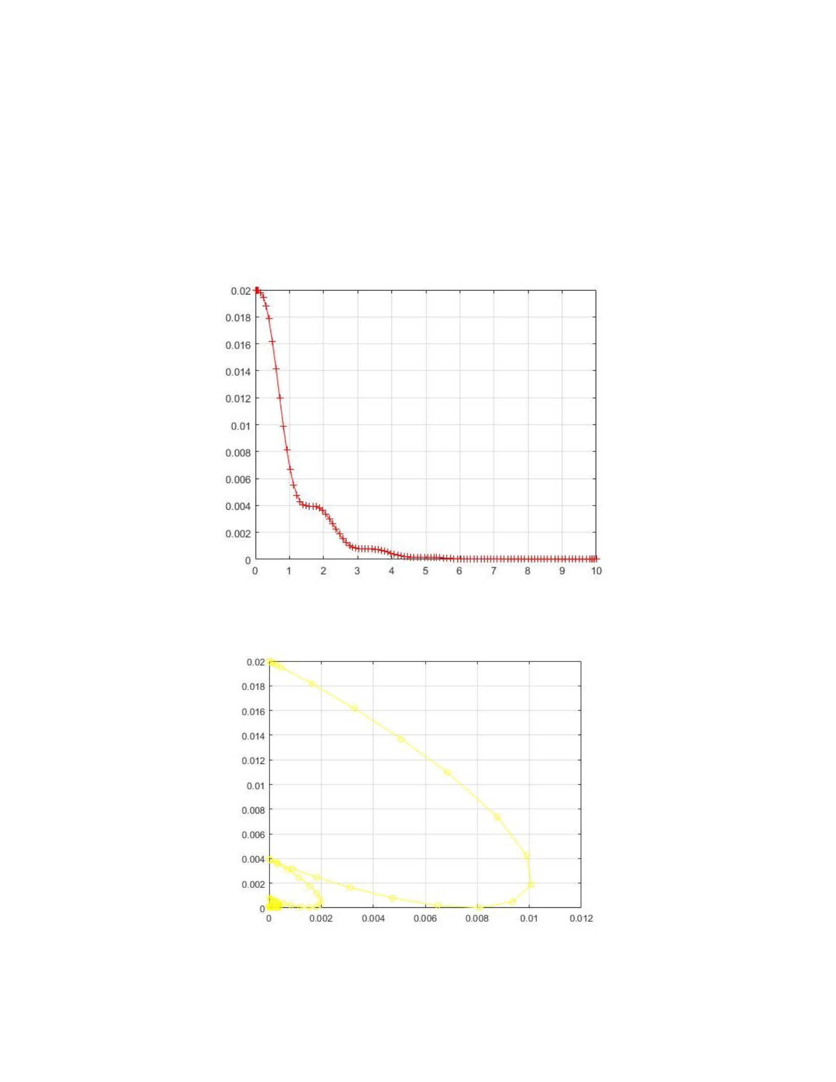
Energy is not conserved in this case because of the coefficient of
friction. The total energy of the system goes down from 0.02 until it is at
rest, and potential must be applied to the system (by stretching the spring)
in order for energy to exist in the system again.
Total Energy of System vs Time
Kinetic vs Potential Energy
b) If the derivative of Energy is negative, the system would be losing energy
due to friction. So, if c>0, the frictional force is going to create a
negative derivative for energy. Alternatively, if the derivative of Energy is
positive, and c<0, then there is a force acting on the system that speeds it
up.
c)
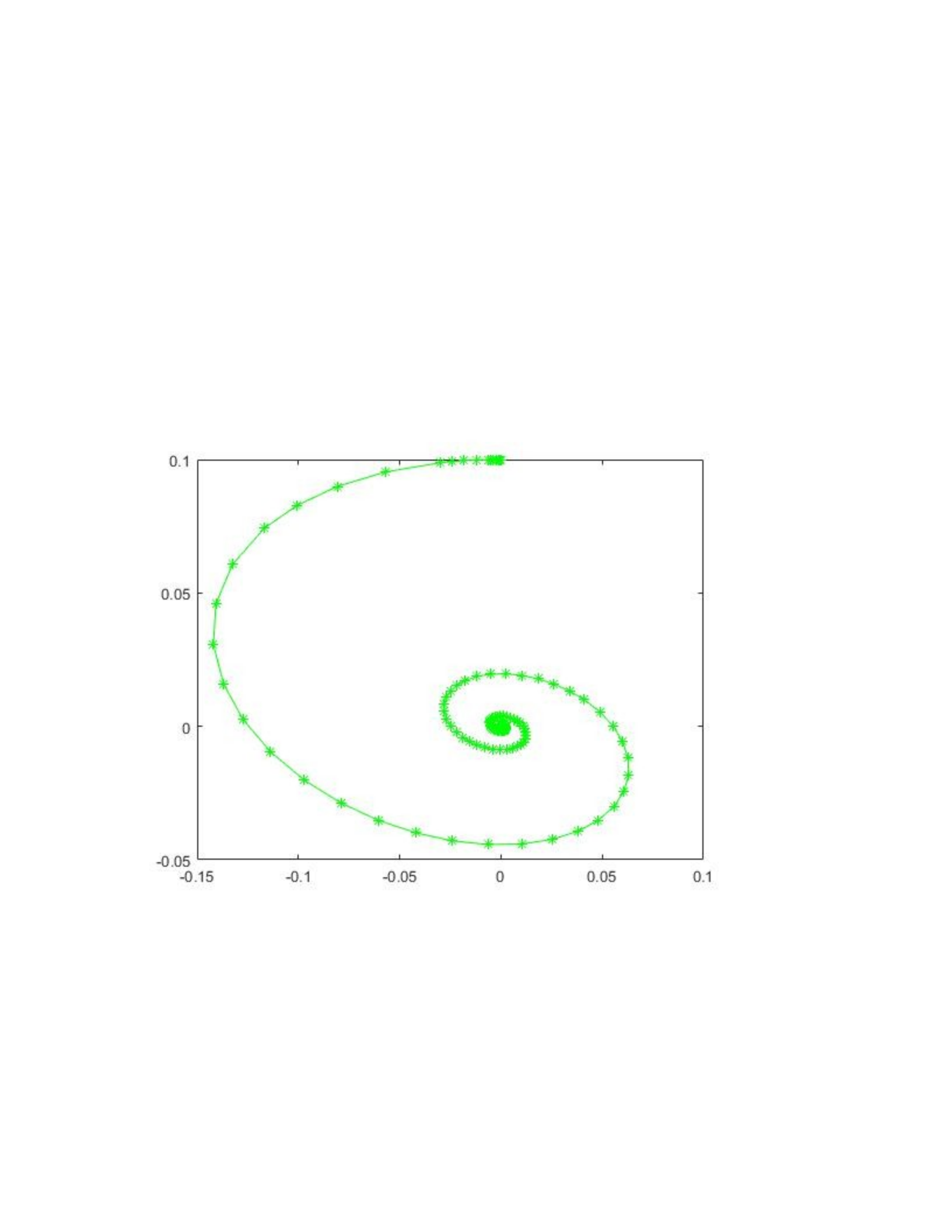
In this case, with the dampening of the system, the phase plot (figure 4)
shows that that curve gets closer to the origin, because with each
movement of the mass, it is losing energy due to friction. This means that
the system will eventually come to rest, unlike the first system where the
mass was perpetually in motion, meaning it stayed in the same pattern of
motion and did not lose or gain total energy.
Figure 4: Phase Plot of v vs y

