



Output of the diary file:
% MAT 275 MATLAB Assignment #3
Exercise 1
% Part A of Exercise 1
f=inline('2*y','t','y'); % defining f as an inline function
t=linspace(0,.5,100); % defining t
y=3*exp(2*t); % defines the exact solution of the ODE
% Using Euler Method to solve the ODE and record the solution in y5
[t5,y5]=euler(f,[0,.5],3, 5); % solves the ODE using Euler with 5
steps
% Using Euler Method to solve the ODE and record the solution in y50
[t50,y50]=euler(f,[0,.5],3, 50); % solves the ODE using Euler with 50
steps
% Using Euler Method to solve the ODE and record the solution in y500
[t500, y500] = euler(f, [0, 0.5], 3, 500); % solves the ODE using
Euler with 500 steps
% Using Euler Method to solve the ODE and record the solution in y5000
[t5000, y5000] = euler(f, [0, 0.5], 3, 5000); % solves the ODE using
Euler with 5000 steps
y5(end); % approximate value with N = 5 (t=0.5)
y50(end); % approximate value with N = 50 (t=0.5)
y500(end); % approximate value with N = 500 (t=0.5)
y5000(end); % approximate value with N = 5000 (t=0.5)
% Estimating the errors i.e. the difference between the actual value
and the approximated value given by Euler method
% Error when N = 5
e5 = y(end) - y5(end);
% Error when N = 50
e50 = y(end) - y50(end);
% Error when N = 500
e500 = y(end) - y500(end);
% Error when N = 5000
e5000 = y(end) - y5000(end);
% Estimating the ratio of the errors at different N
r5 = e5/e50; % Ratio of e5 to e50
r50 = e50/e500; % Ratio of e50 to e500
r500 = e500/e5000; % Ratio of e500 to e5000
% Results for Exercise 1 – Part A
Filling the table with the outputs of the above script
N
Approximation
Error (e)
Ratio (r)
5
7.4650
0.6899
-
50
8.0748
0.0801
8.6148
500
8.1467
0.0081
9.8381
5000
8.1540
8.1534 x10⁻⁴
9.9835
% Part B of Exercise 1
How does the ratio of consecutive errors relate to the number of steps used?
As ‘N’ increases the ratio of consecutive errors also increases. This states that as the number of
steps are increased, Euler method tries to minimize the error (as the ratio of consecutive errors
increases). Also a quick look at column 3 (Error) suggests that as the step size is decreased from
5000 to 500, error also is also changed by the same factor (here 5000/500). This indicates that
the Euler method is of order ‘h’ that is everytime the step size is decreased by a factor (k), error
also changes by the same factor (k).
% Part C of Exercise 1
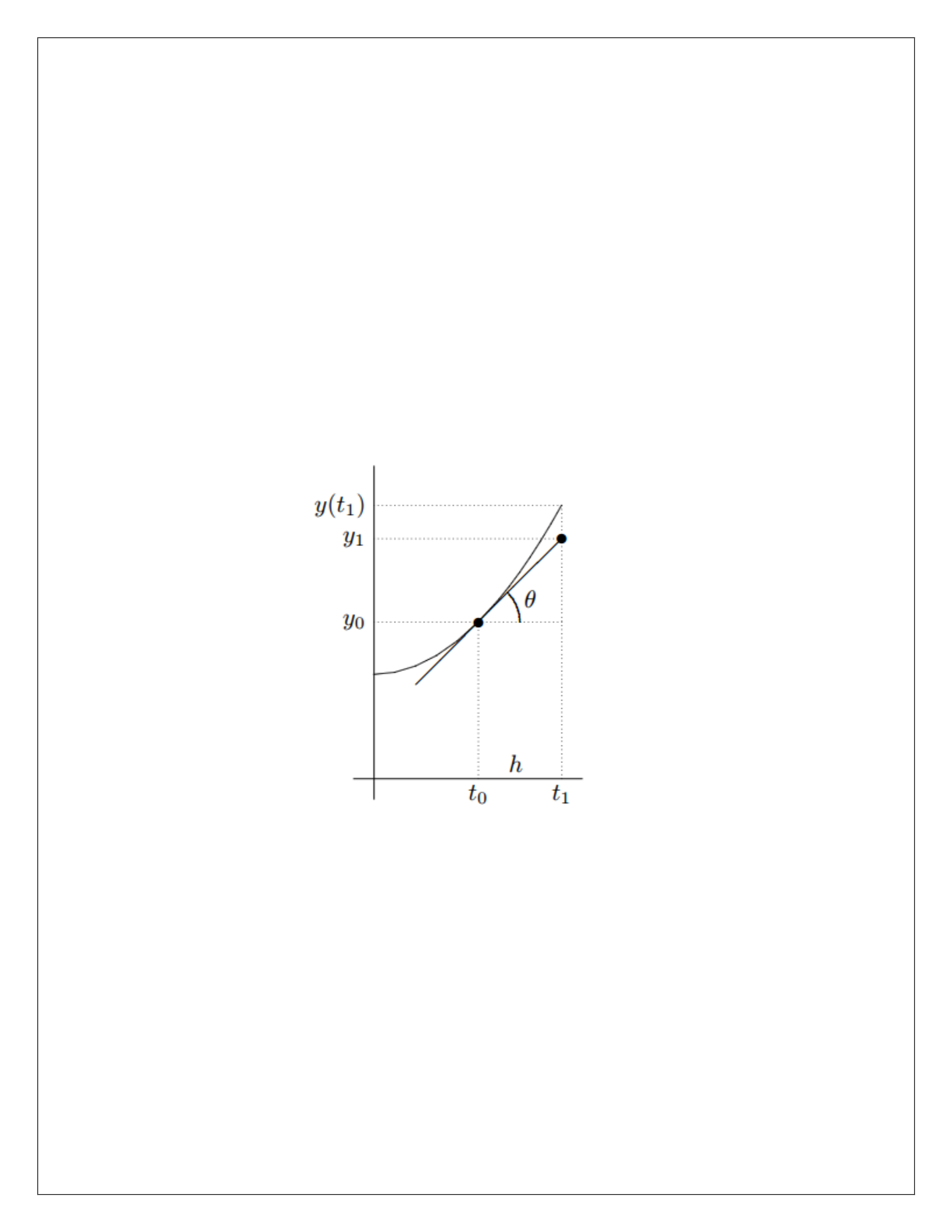
Geometrically, the approximation made is equivalent to replacing the solution curve by the
tangent line at (t0, y0). The geometric interpretation of the Euler’s Method is shown below -
If the point y1 is used to approximate the value of the curve at point y0 then our approximation
will have some error in it. Clearly, the point is not close to y0. For the approximation to have less
error it is required that the point on the tangent curve should be close to the actual curve. This
depends on the step size as well as on the number of steps taken. As the step size decreases (or
the number of steps increases) the point y1 starts getting closer to the point y0 thus, the
approximate value will have less error in it. This is what Euler Method does, it starts at some
point and then keeps on increasing the number of steps to minimize the error. point closer to
the actual curve depending on the step size.
Exercise 2
% Part A of Exercise 2
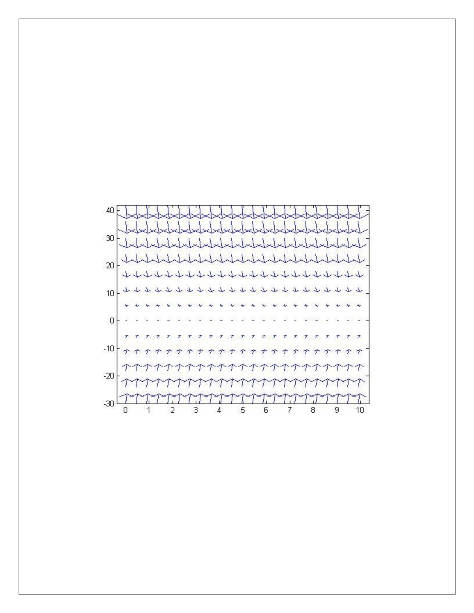
t=0:.45:10; % Defining grid of values in t direction
y = -30:6:42; % Defining grid of values in y direction
[T,Y]=meshgrid(t,y); % Creates 2D matrices of point in ty direction
dT=ones(size(T)); % dt=1 for all the points
dY= -2*Y; % dy=-2*Y – this is the ODE
quiver(T,Y,dT,dY); % draw arrows (t,y)->(t+dt, t+dy)
axis tight; % Adjust look
hold on; % Hold ‘on’ to plot on the same figure
% Results for Exercise 2 – Part A
% Part B of Exercise 2
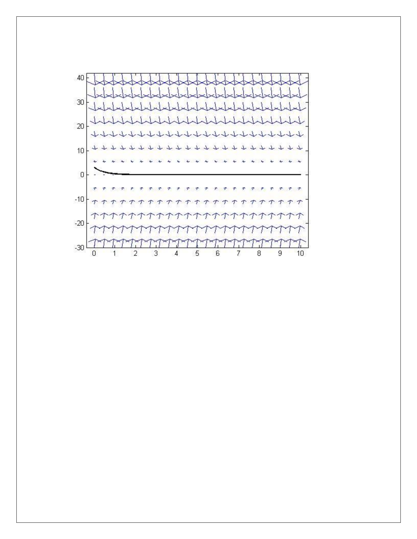
t = linspace(0, 10, 200); % Using linspace to generate ‘t’
y = 3.*exp(-2.*t); % The solution of the ODE
plot(t, y, 'k', 'LineWidth', 2); % Plot the solution in black
% Results for Exercise 2 – Part B
% Part C of Exercise 2
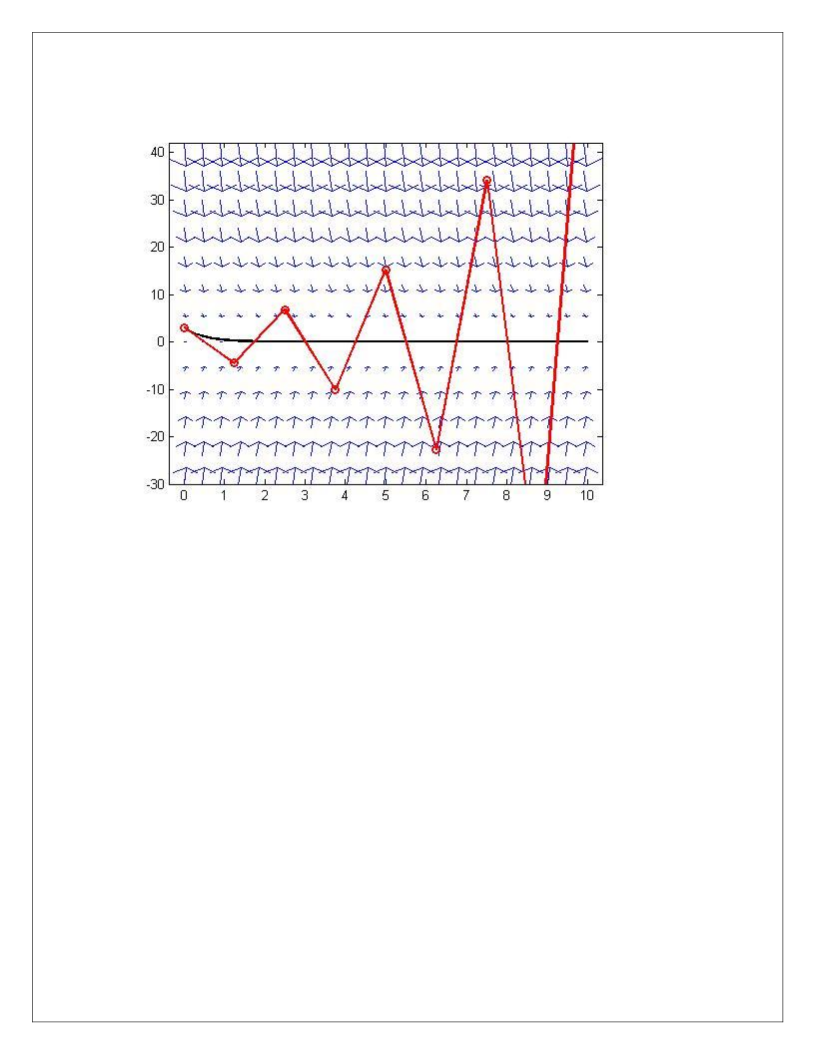
f = inline('-2*y','t','y'); % Using ‘inline’ to define f
[T, Y] = euler(f, [0, 10], 3, 8); % Using ‘euler’ to find solution
plot(T, Y, 'ro-', 'LineWidth', 2); % Final plot in red of the solution
% Results for Exercise 2 – Part C
% Part D of Exercise 2
figure; % To open a new figure
t=0:.4:10; % Defining grid of values in t direction
y = -1:0.4:3; % Defining grid of values in y direction
[T,Y]=meshgrid(t,y); % Creates 2D matrices of point in ty direction
dT=ones(size(T)); % dt=1 for all points
dY= -2*Y; % dy=-2*Y – this is the ODE
quiver(T,Y,dT,dY); % draw arrows
axis tight; % adjust looks
hold on; % Turn hold on
t = linspace(0, 10, 200); % Using linspace to generate ‘t’
y = 3.*exp(-2.*t); % The solution of ODE
plot(t, y, 'k', 'LineWidth', 2); % Plot the solution in black
f = inline('-2*y','t','y'); % Define ‘f’ using inline function
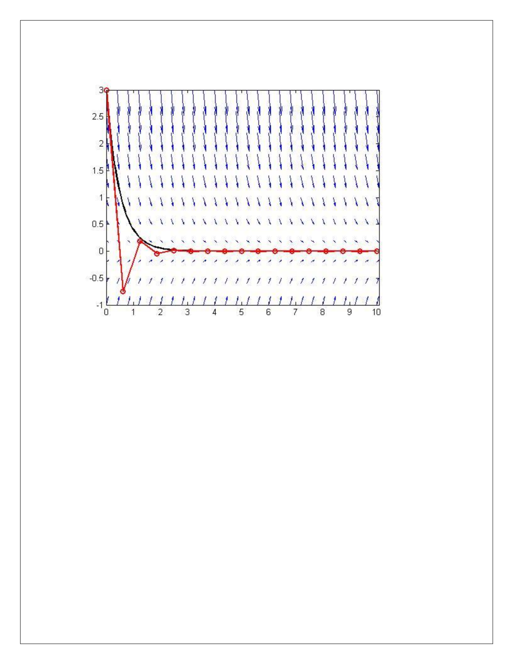
[T, Y] = euler(f, [0, 10], 3, 16); % Use Euler to find the solution
plot(T, Y, 'ro-', 'LineWidth', 2); % Plot the solution in Red
% Results for Exercise 2 – Part D
Exercise 3
function [t,y] = impeuler(f,tspan,y0,N)
m = length(y0);
t0 = tspan(1);
tf = tspan(2);
h = (tf-t0)/N; % Calculating the time step size
t = linspace(t0,tf,N+1); % Defining the variable ‘t’
y = zeros(m,N+1); % Defining the output variable ‘y’
y(:,1) = y0'; % Setting initial conditions
for n=1:N
% Implement Improved Euler’s method on each n = 1 to N
y(:,n+1) = y(:,n) + (h/2)*( f(t(n), y(:, n)) + f(t(n) + h, y(:, n) +
h* f(t(n), y(:, n))));
end
t = t'; % change t from row to column vector
y = y'; % change y from row to column vector
end

% Results for Exercise 3
>> f = inline('2*y','t','y');
>> [t5,y5] = impeuler(f,[0,.5],3,5);
>> [t5, y5]
ans =
0 3.0000
0.1000 3.6600
0.2000 4.4652
0.3000 5.4475
0.4000 6.6460
0.5000 8.1081
Exercise 4
% Part A of Exercise 4
f=inline('2*y','t','y'); % defining f as an inline function
t=linspace(0,.5,100); % defining t
y=3*exp(2*t); % defines the exact solution of the ODE
% Using ImpEuler Method to solve the ODE and record the solution in y5
[t5,y5]=impeuler(f,[0,.5],3, 5); % solves the ODE using Impeuler with
5 steps
% Using Impeuler Method to solve the ODE and record the solution in
y50
[t50,y50]=impeuler(f,[0,.5],3, 50); % solves the ODE using ImpEuler
with 50 steps
% Using Impeuler Method to solve the ODE and record the solution in
y500
[t500, y500] = impeuler(f, [0, 0.5], 3, 500); % solves the ODE using
Impeuler with 500 steps
% Using Impeuler Method to solve the ODE and record the solution in
y5000
[t5000, y5000] = impeuler(f, [0, 0.5], 3, 5000); % solves the ODE
using Impeuler with 5000 steps
y5(end); % approximate value with N = 5 (t=0.5)
y50(end); % approximate value with N = 50 (t=0.5)
y500(end); % approximate value with N = 500 (t=0.5)
y5000(end); % approximate value with N = 5000 (t=0.5)
% Estimating the errors i.e. the difference between the actual value
and the approximated value given by Impeuler method
% Error when N = 5
e5 = y(end) - y5(end);
% Error when N = 50
e50 = y(end) - y50(end);
% Error when N = 500
e500 = y(end) - y500(end);
% Error when N = 5000
e5000 = y(end) - y5000(end);

% Estimating the ratio of the errors at different N
r5 = e5/e50; % Ratio of e5 to e50
r50 = e50/e500; % Ratio of e50 to e500
r500 = e500/e5000; % Ratio of e500 to e5000
% Results for Exercise 4 – Part A
Filling the table with the outputs of the above script
N
Approximation
Error(e)
Ratio(r)
5
8.1081
0.0467
-
50
8.1543
5.3555x10⁻⁴
87.2394
500
8.1548
5.4284 x10⁻⁶
98.6567
5000
8.1548
5.4357 x10⁻⁸
99.8650
% Part B of Exercise 4
How does the ratio of consecutive errors relate to the number of steps used?
As ‘N’ increases the ratio of consecutive errors also increases. This states that as the number of
steps are increased, Improved Euler method tries to minimize the error (as the ratio of
consecutive errors increases). Also a quick look at column 3 (Error) suggests that as the step
size is decreased from 5000 to 500, error is approximately changed by the square of the factor
(here 5000/500). This indicates that the Improved Euler method is of order ‘h2’ that is
everytime the step size is decreased by a factor (k), error changes by the square of the factor
(k).
Exercise 5
% Part A of Exercise 5
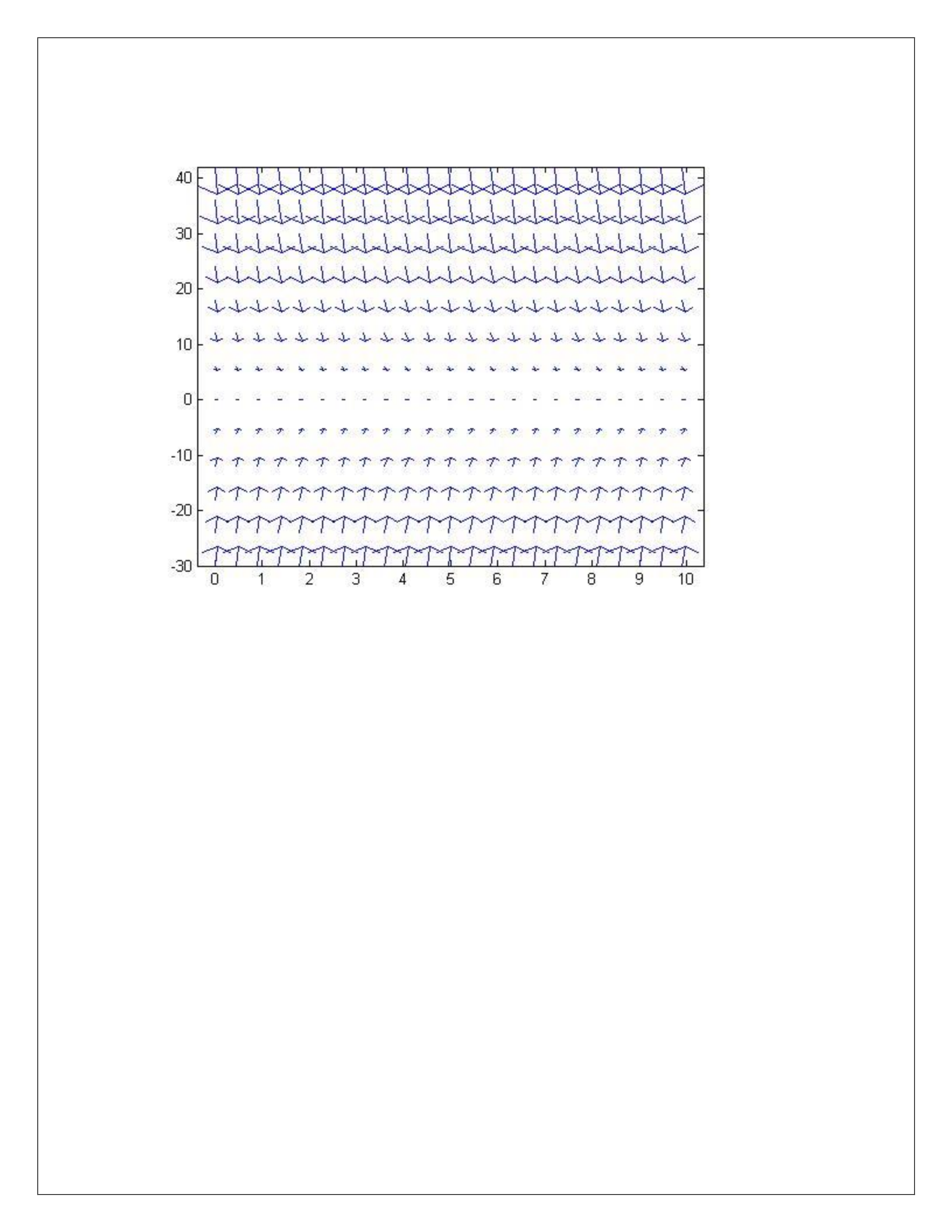
t=0:.45:10; % Defining grid of values in t direction
y = -30:6:42; % Defining grid of values in y direction
[T,Y]=meshgrid(t,y); % Creates 2D matrices of point in ty direction
dT=ones(size(T)); % dt=1 for all the points
dY= -2*Y; % dy=-2*Y – this is the ODE
quiver(T,Y,dT,dY); % draw arrows (t,y)->(t+dt, t+dy)
axis tight; % Adjust look
hold on; % Hold ‘on’ to plot on the same figure
% Results for Exercise 5 – Part A
% Part B of Exercise 5
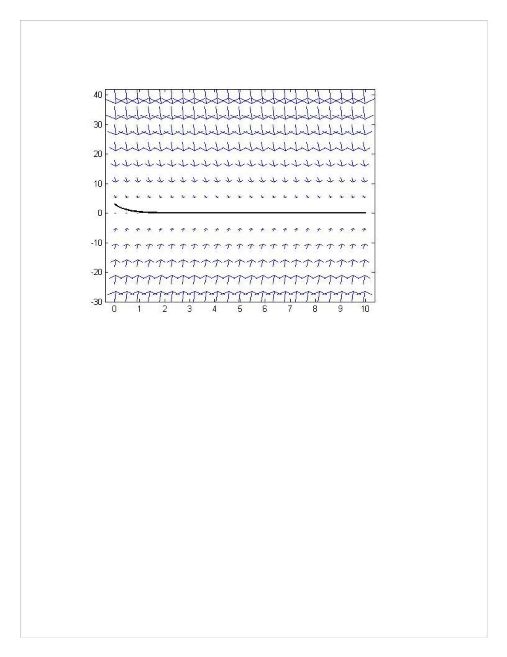
t = linspace(0, 10, 200); % Using linspace to generate ‘t’
y = 3.*exp(-2.*t); % The solution of the ODE
plot(t, y, 'k', 'LineWidth', 2); % Plot the solution in black
% Results for Exercise 5 – Part B
% Part C of Exercise 2
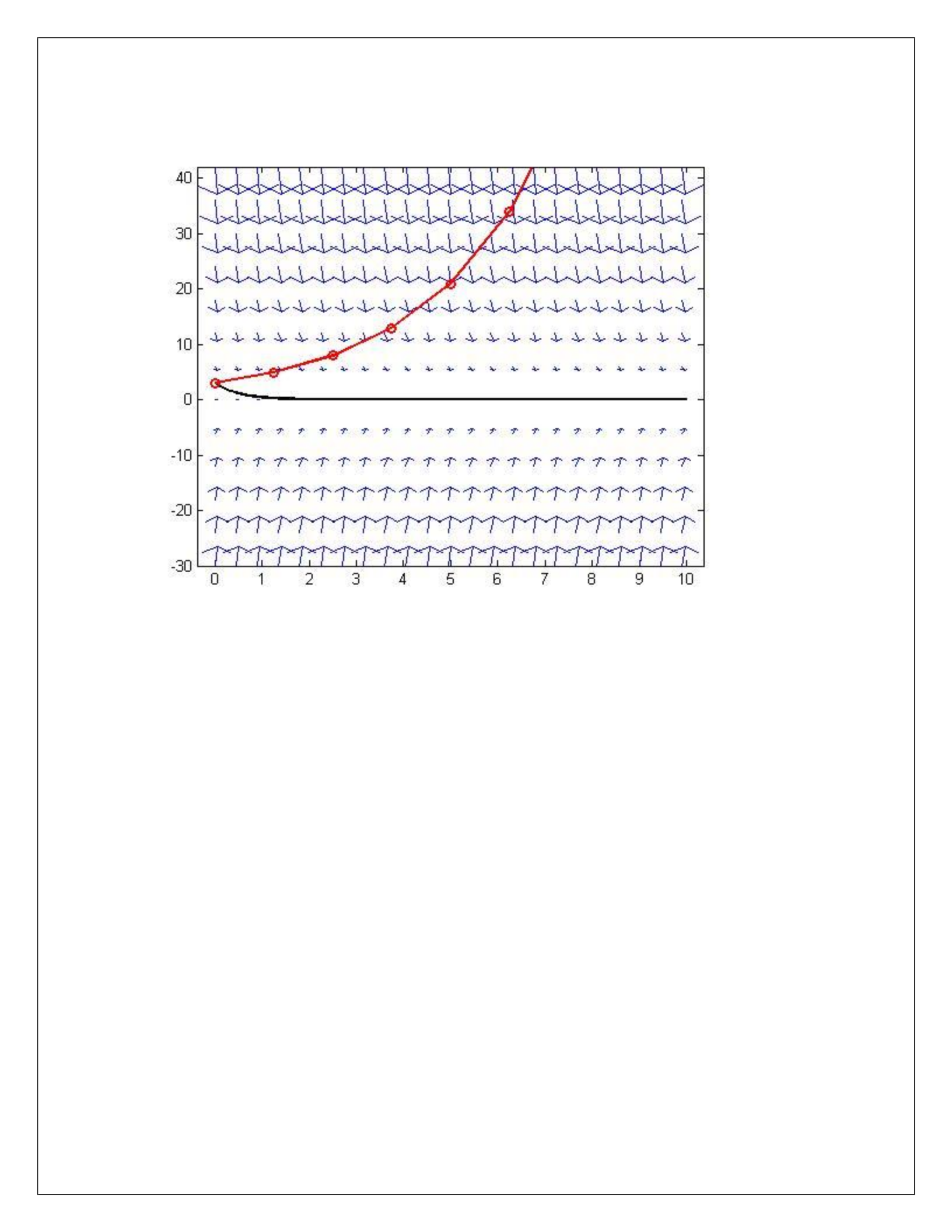
f = inline('-2*y','t','y'); % Using ‘inline’ to define f
[T, Y] = impeuler(f, [0, 10], 3, 8); % Using ‘impeuler’ to find solution
plot(T, Y, 'ro-', 'LineWidth', 2); % Final plot in red of the solution
% Results for Exercise 5 – Part C
% Part D of Exercise 5
figure; % To open a new figure
t=0:.4:10; % Defining grid of values in t direction
y = -1:0.4:3; % Defining grid of values in y direction
[T,Y]=meshgrid(t,y); % Creates 2D matrices of point in ty direction
dT=ones(size(T)); % dt=1 for all points
dY= -2*Y; % dy=-2*Y – this is the ODE
quiver(T,Y,dT,dY); % draw arrows
axis tight; % adjust looks
hold on; % Turn hold on
t = linspace(0, 10, 200); % Using linspace to generate ‘t’
y = 3.*exp(-2.*t); % The solution of ODE
plot(t, y, 'k', 'LineWidth', 2); % Plot the solution in black
f = inline('-2*y','t','y'); % Define ‘f’ using inline function
[T, Y] = impeuler(f, [0, 10], 3, 16); % Use Impeuler to find the solution
plot(T, Y, 'ro-', 'LineWidth', 2); % Plot the solution in Red
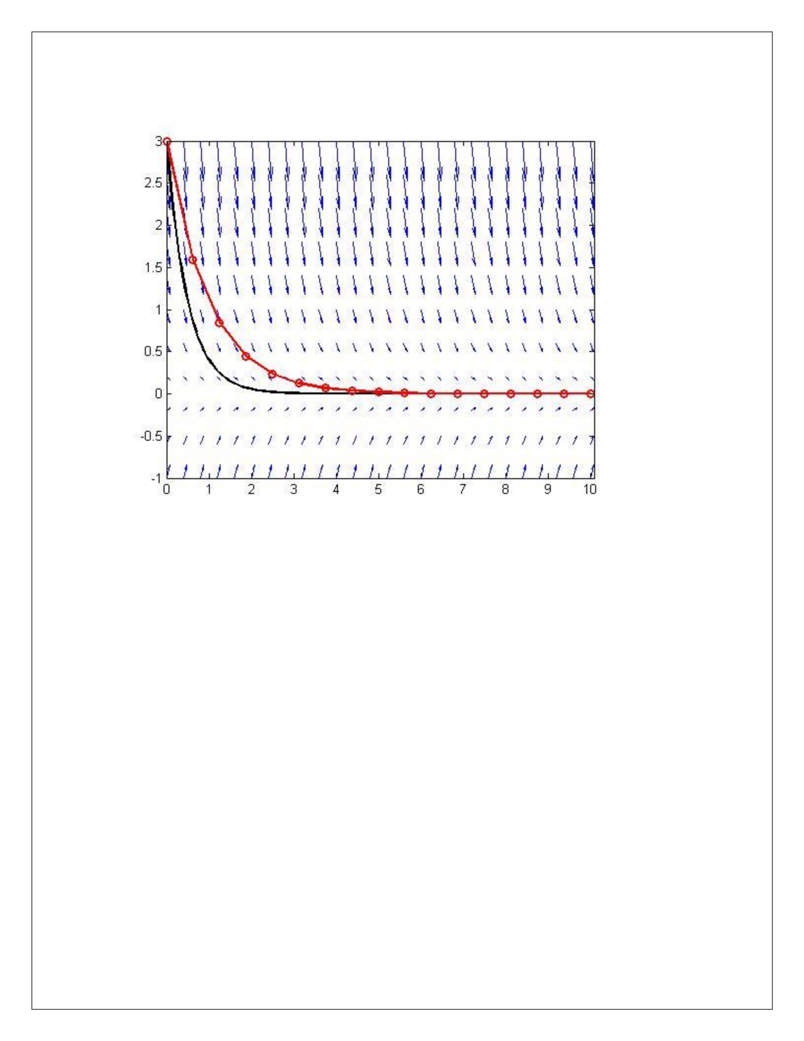
% Results for Exercise 5 – Part D

