



1
Table of Contents
........................................................................................................................................ 1
Excercise 1 ........................................................................................................................ 1
Excercis 2 .......................................................................................................................... 3
Excercise 3 ........................................................................................................................ 5
Excercise 4 ........................................................................................................................ 6
Excercise 5 ........................................................................................................................ 8
%%Alexander Laksono - MAT275 - LAB 3
Excercise 1
%Part a
f=inline('2*y','t','y'); %Define f as an inline function 2y, t, and y
t=linspace(0,.5,100); y=3*exp(2*t); %Define t as the exact solution of the
%ODE as well as creating a vector of t values
[t5,y5]=euler(f,[0,.5],3, 5); %Solves the ODE with Euler's method using
%5 steps
[t5(:), y5(:)];
[t50,y50]=euler(f,[0,.5],3, 50); %Solves the ODE with Euler's method using
%50 steps
[t50(:), y50(:)];
[t500,y500]=euler(f,[0,.5],3, 500);%Solves the ODE with Euler's method
%using 500 steps
[t500(:), y500(:)];
[t5000,y5000]=euler(f,[0,.5],3, 5000);%Solves the ODE with Euler's method
%using 5000 steps
[t5000(:), y5000(:)];
y5(end) %Exact value of the function at t=5
y50(end) %Exact value of the function at t=50
y500(end) %Exact value of the function at t=500
y5000(end) %Exact value of the function at t=5000
error5 = y(end)-y5(end) %Error in using 5 steps
error50 = y(end)-y50(end) %Error in using 50 steps
error500 = y(end)-y500(end) %Error in using 500 steps
error5000 = y(end)-y5000(end) %Error in using 5000 steps
ratio5and50 = error5/error50 %Ratio between error in 5 steps and 50 steps
ratio50and500 = error50/error500 %Ratio between error in 50 steps and 500
%steps
ratio500and5000 = error500/error5000 %Ratio between error in 500 steps and
%5000 steps
%Part b
%The errors is related to the number of step used
%if more step is used, the errors will be smaller, while less step is
%used, the errors will vbe bigger.

2
%Part c
ans =
7.4650
ans =
8.0748
ans =
8.1467
ans =
8.1540
error5 =
0.6899
error50 =
0.0801
error500 =
0.0081
error5000 =
8.1534e-04
ratio5and50 =
8.6148
ratio50and500 =
9.8381

3
ratio500and5000 =
9.9835
Excercis 2
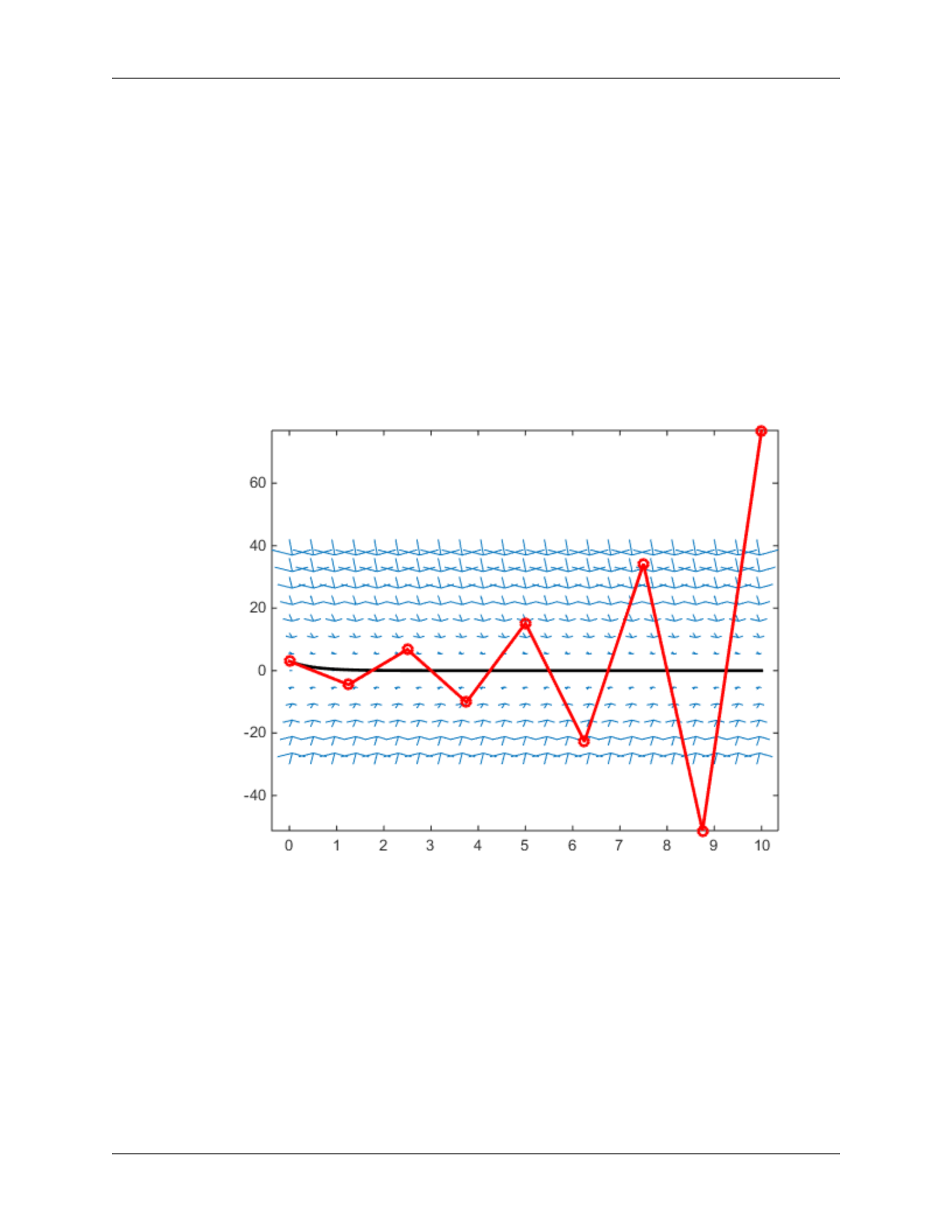
%Part (a)
figure (1) %Command for creating graph figure 1
t = 0:.45:10; y = -30:6:42 ; %define t and y as a grid of values in t and
%y direction
[T,Y]=meshgrid(t,y); %creates 2d matrices of points in the ty-plane
dT = ones(size(T)); %dt=1 for all points
dY = -2*Y; %dy = -2*y; this is the ODE
quiver(T,Y,dT,dY) %draw arrows (t,y)->(t+dt, t+dy)
axis tight %command to adjusting the look of the graph
hold on
%Part (b)
t = linspace(0, 10, 200); %generate a vector of 200 t-values between 0 to
%10
y=3*exp(-2*t); %Evaluating the solution y at values t
plot (t,y,'k','linewidth',2)%Plot the solution in black with direction
%field
%Part (c)
type 'euler.m' %Display the commands from file 'euler.m'
f=inline('-2*y','t','y');%Define f as an inline function -2y, t, and y
[t8,y8]=euler(f,[0,10],3, 8); %Solves the ODE with Euler's method using
%8 steps
plot(t8,y8,'ro-','linewidth',2) %Plot the approximated points in red
%Part (d)
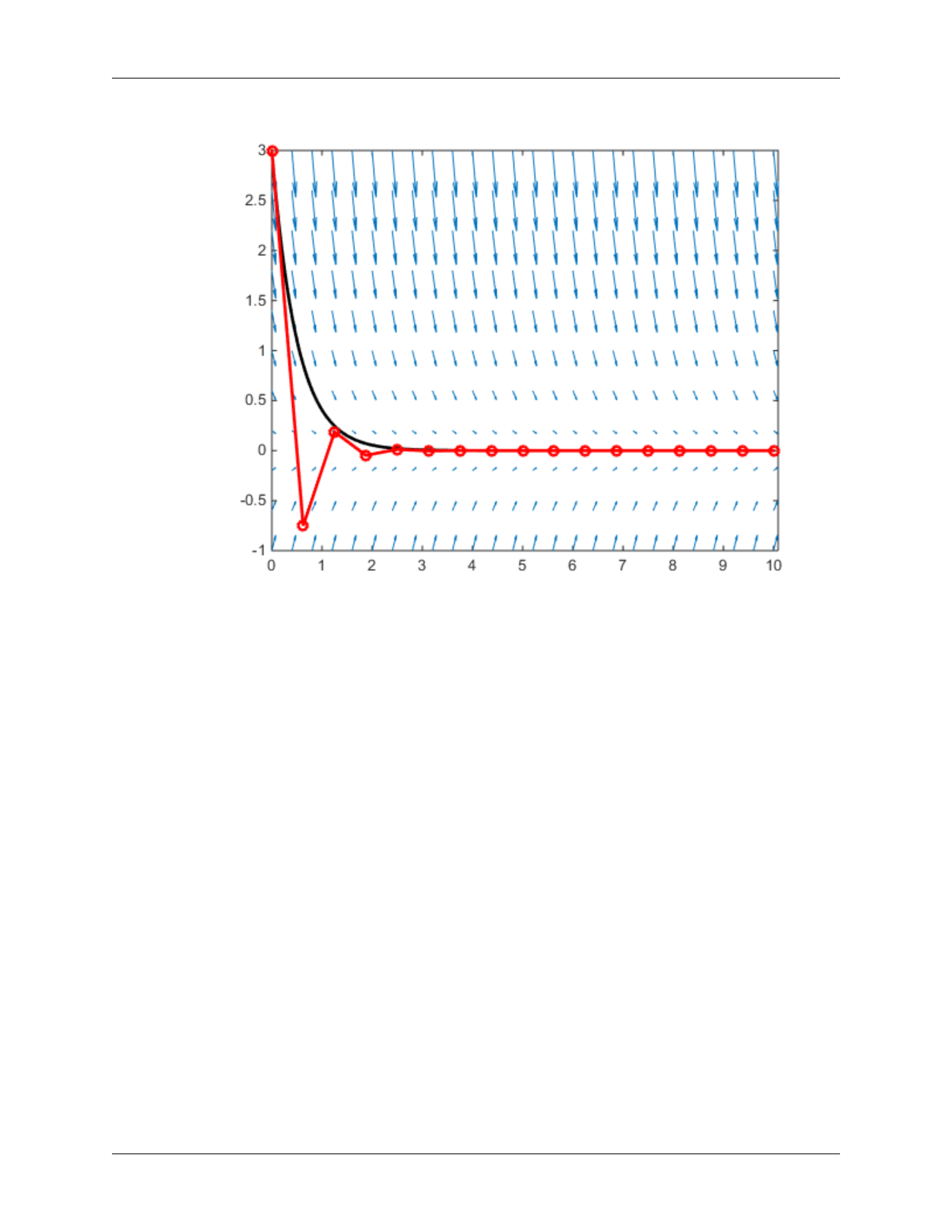
%The whole Part d is similar to the previous parts but with 16 steps
%instead
figure (2)
t = 0:.4:10; y = -1:0.4:3; % define grid of values in t and y direction
[T,Y]=meshgrid(t,y); % creates 2d matrices of points in the ty-plane
dT = ones(size(T)); % dt=1 for all points
dY = -2*Y; % dy = -2*y; this is the ODE
quiver(T,Y,dT,dY) % draw arrows (t,y)->(t+dt, t+dy)
axis tight % adjust look
hold on
t = linspace(0, 10, 200); %generate a vector of 200 t-values between 0 to
%10
y=3*exp(-2*t); %Evaluating the solution y at values t
plot (t,y,'k','linewidth',2) %Plotting t and function y
f=inline('-2*y','t','y');%Define f as an inline function -2y, t, and y
[t16,y16]=euler(f,[0,10],3, 16);%Solves the ODE with Euler's method using
%16 steps instead of 8
plot(t16,y16,'ro-','linewidth',2) %plot the apporximated point in red
4
function [t,y] = euler(f,tspan,y0,N)
m = length(y0);
t0 = tspan(1);
tf = tspan(2);
h = (tf-t0)/N; %evaluating the time step size used
t = linspace(t0,tf,N+1); %define t as a vector of t values
y = zeros(m,N+1);%allocate memory for the output y
y(:,1) = y0';%set initial condition
for n=1:N
y(:,n+1) = y(:,n) + h*f(t(n),y(:,n));%implement Euler's method
end
t = t'; y = y';%change t and y from row to column vectors
end
5
Excercise 3
type 'improvedeuler.m'%Display the commands from file "improvedeuler.m"
%the modified version of file "euler.m"
f=inline('2*y','t','y');%Define f as an inline function 2y, t, and y
[t5,y5] = improvedeuler(f,[0,.5],3,5);%Solves the ODE with Euler's method
%using 5 steps
[t5(:),y5(:)]
function [t,y] = improvedeuler(f,tspan,y0,N)
m = length(y0);
t0 = tspan(1);
tf = tspan(2);
h = (tf-t0)/N; % evaluate the time step size
t = linspace(t0,tf,N+1); % create the vector of t values
y = zeros(m,N+1); % allocate memory for the output y
y(:,1) = y0'; % set initial condition
for n=1:N
f1=f(t(n),y(:,n));
f2=f(t(n+1),y(:,n)+h*f1);
y(:,n+1) = y(:,n) + h/2*(f1+f2); % implement Euler's method
end
t = t'; y = y'; % change t and y from row to column vectors
end

6
ans =
0 3.0000
0.1000 3.6600
0.2000 4.4652
0.3000 5.4475
0.4000 6.6460
0.5000 8.1081
Excercise 4
%Part a
f=inline('2*y','t','y');%Define f as an inline function 2y, t, and y
t=linspace(0,.5,100); y=3*exp(2*t);
[t5,y5] = improvedeuler(f,[0,.5],3,5);%Solves the ODE with Euler's method
%using 5 steps
[t5(:), y5(:)];
[t50,y50]=improvedeuler(f,[0,.5],3, 50);%Solves the ODE with Euler's method
%using 5- steps
[t50(:), y50(:)];
[t500,y500]=improvedeuler(f,[0,.5],3, 500);%Solves the ODE with Euler's
%method using 500 steps
[t500(:), y500(:)];
[t5000,y5000]=improvedeuler(f,[0,.5],3, 5000);%Solves the ODE with Euler's
%method using 5000 steps
[t5000(:), y5000(:)];
y5(end)%Exact value of the function at t=5
y50(end)%Exact value of the function at t=50
y500(end)%Exact value of the function at t=500
y5000(end)%Exact value of the function at t=5000
error5 = y(end)-y5(end)%Error in using 5 steps
error50 = y(end)-y50(end)%Error in using 50 steps
error500 = y(end)-y500(end)%Error in using 50 steps
error5000 = y(end)-y5000(end)%Error in using 50 steps
ratio5and50 = error5/error50%Ratio between error in 5 steps and 50 steps
ratio50and500 = error50/error500%Ratio between error in 50 steps and 500
%steps
ratio500and5000 = error500/error5000%Ratio between error in 500 steps and
%5000 steps
%Part b
%te ratio of the errors is increasing as more steps used as the errors is
%getting smaller when larger steps used. Different from the unimproved
%euler, the improved euler method have less errors, also the approximation
%values are closer to each other compared to the unimproved euler, and the
%improved euler have bigger ratio means it is more accurate compared to the
%unimproved euler.

7
ans =
8.1081
ans =
8.1543
ans =
8.1548
ans =
8.1548
error5 =
0.0467
error50 =
5.3555e-04
error500 =
5.4284e-06
error5000 =
5.4357e-08
ratio5and50 =
87.2394
ratio50and500 =
98.6567
ratio500and5000 =
99.8650

8
Excercise 5
%Part a
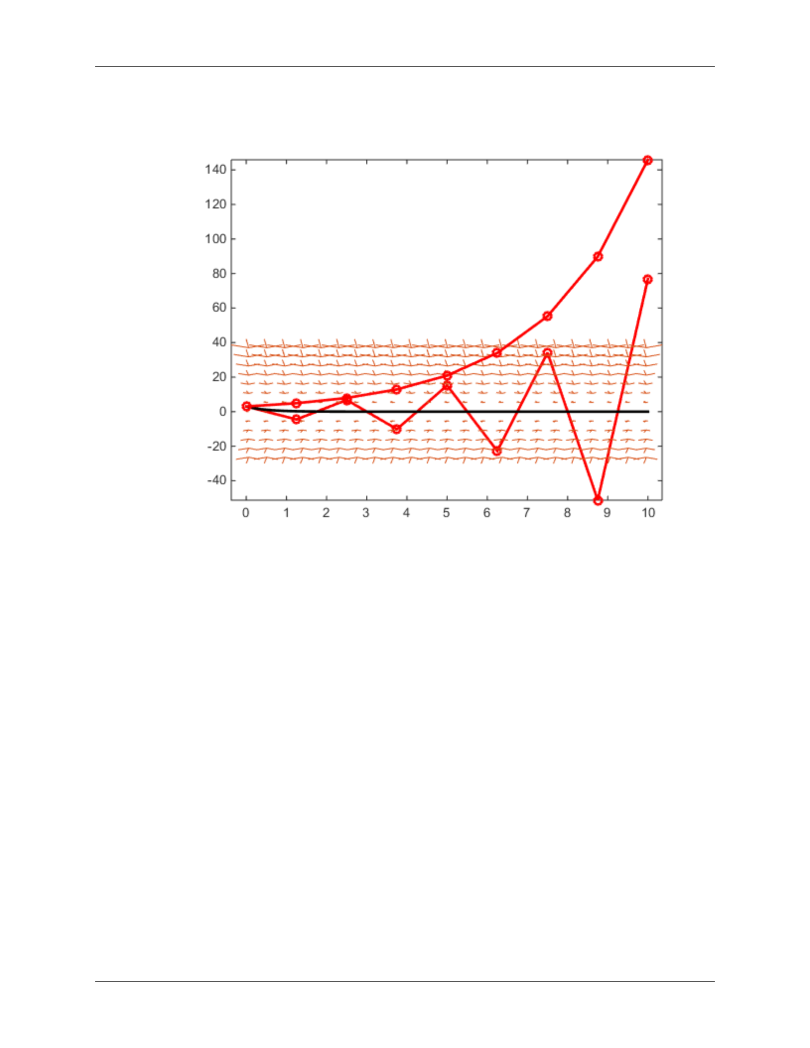
figure (1)
t = 0:.45:10; y = -30:6:42 ; %define t and y as a grid of values in t and
%y direction
[T,Y]=meshgrid(t,y); % creates 2d matrices of points in the ty-plane
dT = ones(size(T)); % dt=1 for all points
dY = -2*Y; % dy = -2*y; this is the ODE
quiver(T,Y,dT,dY) % draw arrows (t,y)->(t+dt, t+dy)
axis tight % command to adjusting the look of the graph
hold on
%Part b
t = linspace(0, 10, 200);
y=3*exp(-2*t); %Evaluating the solution y at values t
plot (t,y,'k','linewidth',2)%Plot the solution in black with direction
%field
%Part c
f=inline('-2*y','t','y');%Define f as an inline function -2y, t, and y
[t8,y8]=improvedeuler(f,[0,10],3, 8);%Solves the ODE with Euler's method
%using 8 steps
plot(t8,y8,'ro-','linewidth',2)
%Part d
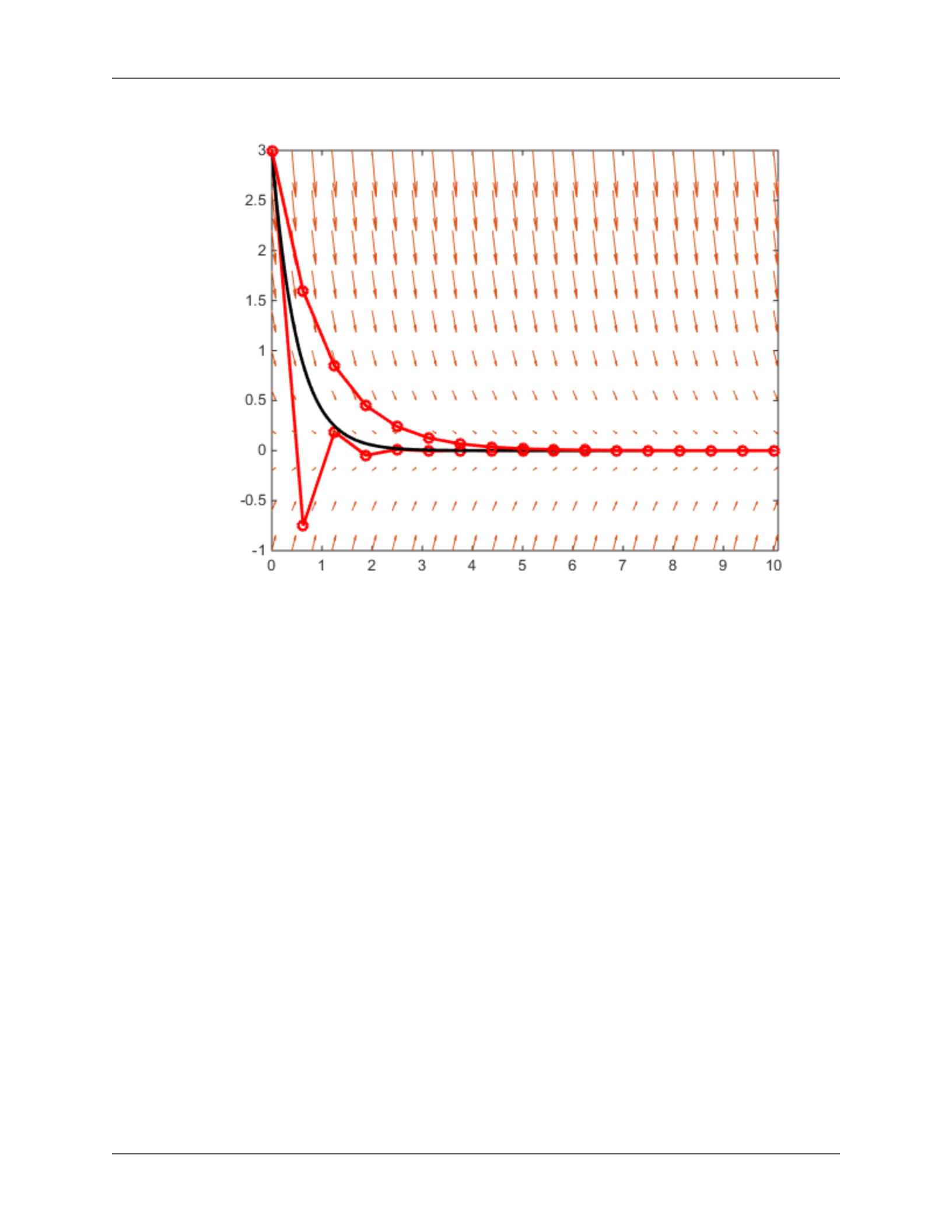
%The whole Part d is similar to the previous parts but with 16 steps
%instead
figure (2)
t = 0:.4:10; y = -1:0.4:3; % define grid of values in t and y direction
[T,Y]=meshgrid(t,y); % creates 2d matrices of points in the ty-plane
dT = ones(size(T)); % dt=1 for all points
dY = -2*Y; % dy = -2*y; this is the ODE
quiver(T,Y,dT,dY) % draw arrows (t,y)->(t+dt, t+dy)
axis tight %command to adjusting the look of the graph
hold on
t = linspace(0, 10, 200); %generate a vector of 200 t-values between 0 to
%10
y=3*exp(-2*t); %Evaluating the solution y at values t
plot (t,y,'k','linewidth',2)%Plotting t and function y
f=inline('-2*y','t','y');%Define f as an inline function -2y, t, and y
[t16,y16]=improvedeuler(f,[0,10],3, 16);%Solves the ODE with Euler's method
% using 16 steps instead of 8
plot(t16,y16,'ro-','linewidth',2)%Plot the approximated points in red
%Comparing the output graph from number 2 (euler) and 5 (improved euler)
%, both graph looks different with graph from number 2 looks way less
%accurate. The graph from number 5 have a curve which graph from number 2
%didn't have on it. The direction field of the graph is simillar from both
140
120
100
40
20
a
\
i
i
oe
cms
A
A
aye
Ay
9
%number 2 and number 5.
10
Published with MATLAB® R2014b

