


Jacob Derr
MAT 275 Lab 5
11/08/2020
Exercise 1
Part a) The blue curve in the Fig, L5a represents
y=y(t). You can tell by looking at the initial
conditions in the MATLAB program that’s given in the
Lab Manual. The initial condition y0 is at 0.1, whereas
v0 is at 0.
Part b) by using omega0 the period comes out to equal
pi. This was found by
ω
0=sqrt(k/m)=sqrt(4/1)=2, T(period)=(2*pi)/2=pi
Part c) No, the mass will not come to a rest. After
looking over the graph, it’s easy to see that the curve
is very uniform, and therefore will keep oscillating.
Usually there will be a damping constant for a mass to
come to rest.
Part d) The amplitude of the oscillations for y is 0.1.
When going from peak to peak it’s 0.2.
Part e) The maximum velocity attained by the mass is
0.2 m/s at t=2,4,5.5,and 8.7 seconds.
Part f) A larger mass results in a stronger force
downward on the spring, and a stiffer spring will make
it less flexible (less oscillations). Looking at the
graphs below, you can see that the period of the m=5
k=4 is greater than the period of m=1 k=16. This means
that bigger mass with small k constant will create a
loner, but slower, oscillation. The lighter mass but
greater spring constant creates a faster, but shorter,
oscillation.
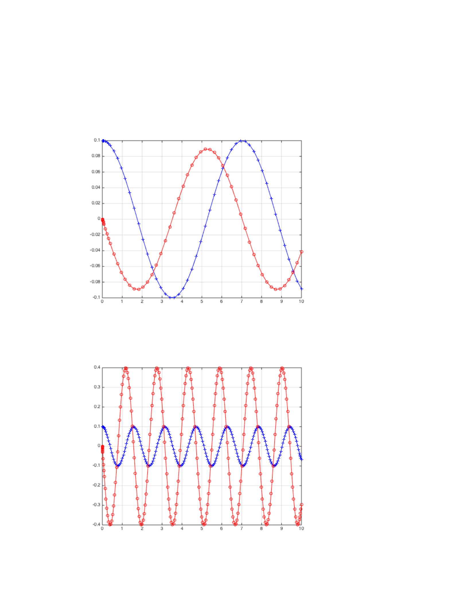
m=5 k=4
m=1 k=16

Exercise 2)
Part a)
function Lab5Q2
m = 1;
k = 4;
omega0=sqrt(k/m);
y0=0.1; v0=0;
[t,Y]=ode45(@f,[0,10],[y0,v0],[],omega0); % solve for
0<t<10
y=Y(:,1); v=Y(:,2);
figure(1); plot(t,y,'b+-',t,v,'ro-');
grid on;
E = .5*m*v.^2 + .5*k*y.^2;
figure(2)
plot(t,E)
legend('Energy')
xlabel('Time')
ylabel('Energy Amount')
ylim([.015,.025])
figure(3)
plot(v,y)
%------------------------------------------------------
function dYdt= f(t,Y,omega0)
y = Y(1); v= Y(2);
dYdt = [v; -omega0^2*y];
end
end
% mass [kg]
% spring constant [N/m]
% initial conditions
% retrieve y, v from Y
% time series for y and v
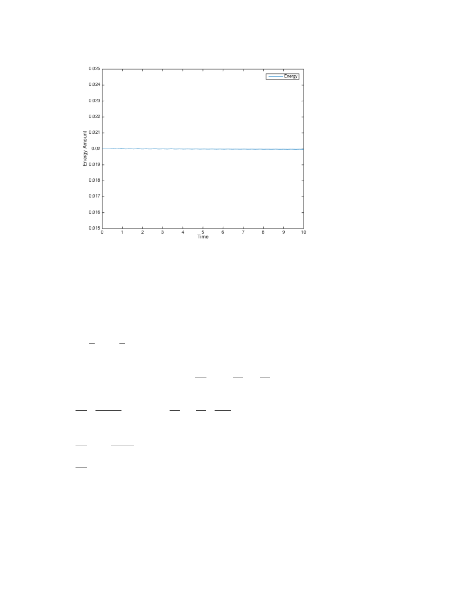
% Looking at the graph above, you can see there is only
a line at 0.02. Yes, energy is conserved.
Part b)
E=1
2m v2−1
2k y2
dE
dt =m∗vdv
dt +ky dx
dt
dE
dt =mv∗dt
dt +ky y'where dy
dt =0, dv
dt =−ky
vt
dE
dt =mv
(
−kmv
y
)
+kyv
dE
dt =ky v −ky v=0
Part c)
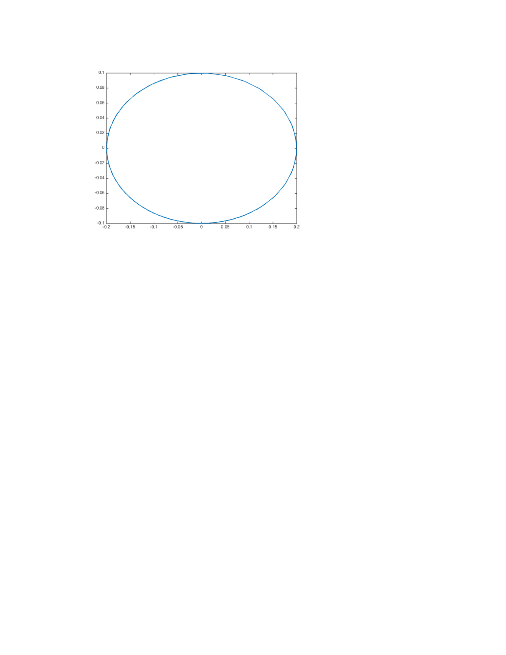
No, the curve doesn’t get close to the origin, because
energy is conserved, meaning that the mass-spring
system goes through an un-damped motion.
Exercise 3
Part a)
function LAB05ex3a
m = 1;
k = 4;
c = 1;
% mass [kg]
% spring constant [N/m]
% friction coefficient [Ns/m]
omega0 = sqrt(k/m); p = c/(2*m);
y0 = 0.1; v0 = 0; % initial conditions
[t,Y]=ode45(@f,[0,10],[y0,v0],[],omega0,p); % solve for
0<t<10
y=Y(:,1); v=Y(:,2); % retrieve
y, v from Y
figure(1); plot(t,y,'b+-',t,v,'ro-'); % time
series for y and v
grid on
%------------------------------------------------------
function dYdt= f(t,Y,omega0,p)
y = Y(1); v= Y(2);
dYdt = [v;-2*p*v-omega0^2*y];
% fill-in dv/dt
Using:
for i=1:length(y)
m(i)=max(abs(y(i:end)));
end
i = find(m<0.01); i = i(1);
disp(['|y|<0.01 for t>t1 with ' num2str(t(i-1)) '<t1<'
num2str(t(i))])
% In the function the minimal time t1 will satisfy |
y(t)|<0.01 for all t>t1 is:
>> LAB05ex3a
|y|<0.01 for t>t1 with 3.7807<t1<3.8711
Part b)

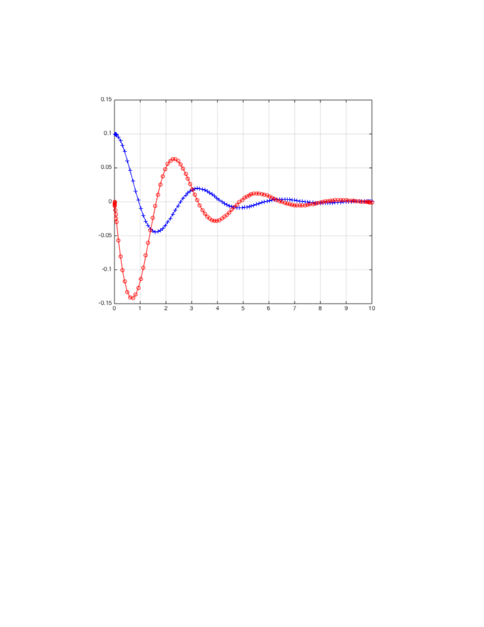
By zooming into the graph above, it’s easy to see both
the maximum velocity attained and the time when it is
attained.
T=0.7148s and v=0.142m/s
Part c)
The size of c affects the motion by damping it. This
means that the velocity will decrease as c increases.
c=2
c=4
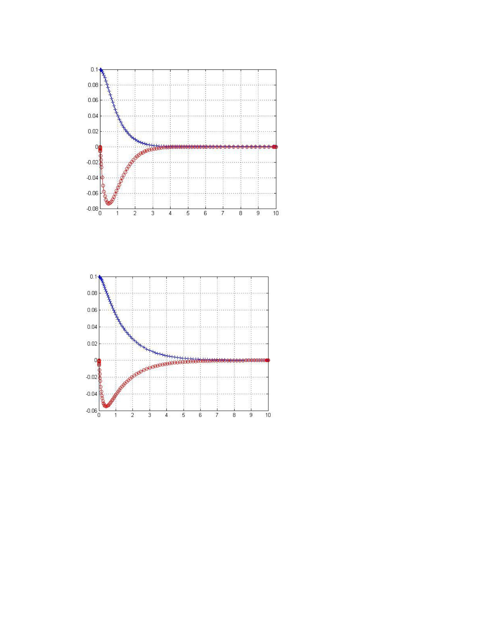
c=6
c=8
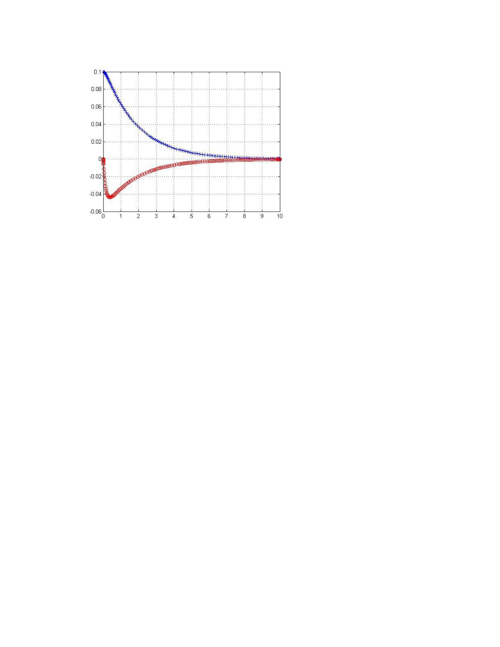
Part d)
The smallest value of c such that no oscillation
appears in the solution is
c = sqrt(4mk)
c^2 = 4mk
c^2 = 4*1*4
c^2 = 16
c = sqrt(16)
c = 4
Exercise 4
Part a)
function LAB05ex1a
m = 1;
k = 4;
c = 1;
% mass [kg]

% spring constant [N/m]
% friction coefficient [Ns/m]
omega0 = sqrt(k/m); p = c/(2*m);
y0 = 0.1; v0 = 0; % initial conditions
[t,Y]=ode45(@f,[0,10],[y0,v0],[],omega0,p); % solve for
0<t<10
y=Y(:,1); v=Y(:,2);
figure(1); plot(t,y,'b+-',t,v,'ro-');
grid on
E = .5*m*v.^2 + .5*k*y.^2;
figure(2)
plot(t,E)
legend('Energy')
xlabel('Time')
ylabel('Energy Amount')
ylim([.015,.025])
figure(3)
plot(v,y)
%------------------------------------------------------
function dYdt= f(t,Y,omega0,p)
y = Y(1); v= Y(2);
dYdt = [v;-2*p*v-omega0^2*y];
end
end
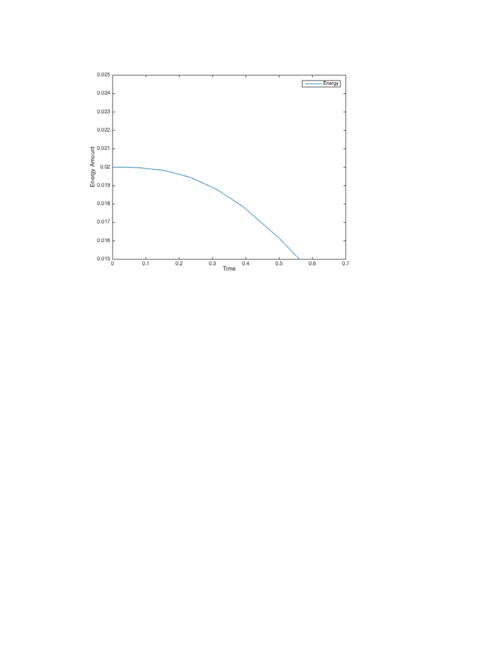
Looking at the graph above, it’s easy to see that it
goes to 0 and energy is not conserved.
Part b)
E=.5 m v2+.5 k y2
E'=mv v'+ky y'
E'=v
(
−ky −c y'
)
+kvy
E'=v
(
−ky −c y'+ky
)
c=4c=−4
E'=−4'v∨E'=4y'v
Part c)
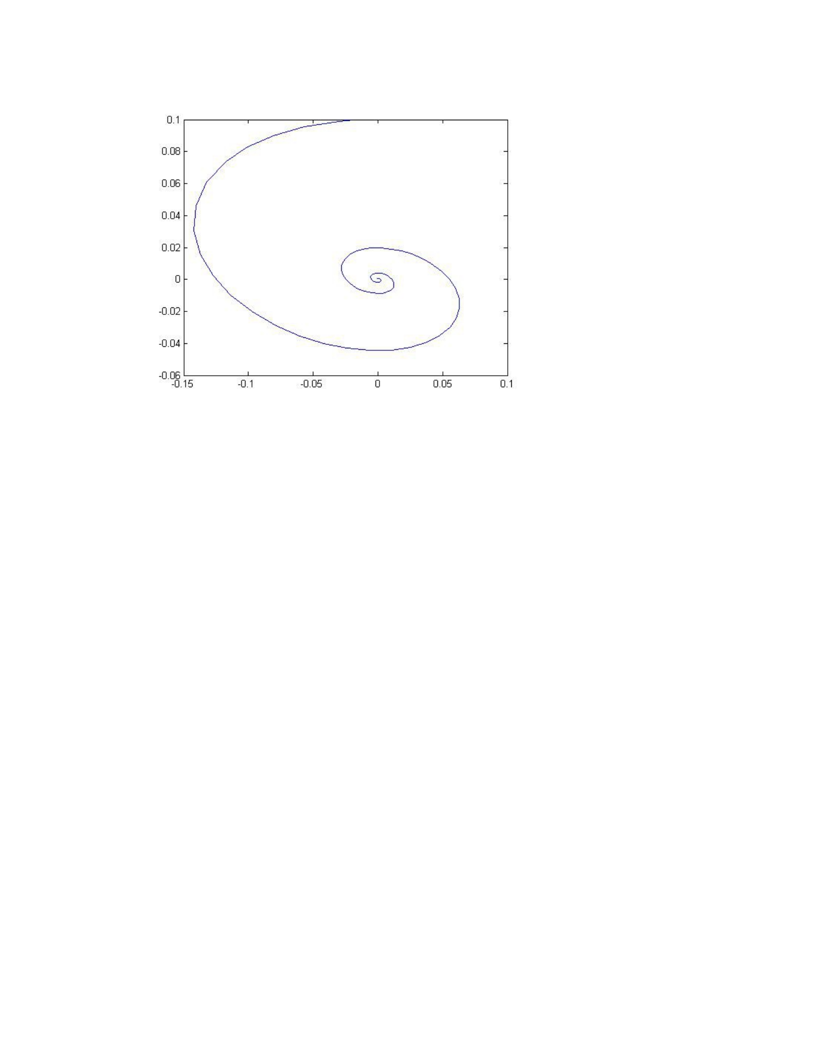
The curve is a spiral and will ultimately reach the
origin at some point in time. It will continue to
oscillate, becoming smaller and smaller, until it
finally stops. This is because of the damping constant.

