


MAT 275 - MATLAB Assignment #6
% Question 1
The behavior of the forced oscillations as per the figure L6a is identical to a sinusoidal
waveform. Therefore, by the method of visual inspection we can calculate the time period
approximately as 4.5secs. Also on using the equation L6.4 {with the case when ω0 > ω} α =
0.601 radians.
% Output (B)
Updating the function LAB06ex1 to meet the requirements -
function LAB06ex1
omega0 = 2; c = 1; omega = 1.4;
param = [omega0,c,omega];
t0 = 0; y0 = 0; v0 = 0; Y0 = [y0;v0]; tf = 50;
options = odeset('AbsTol',1e-10,'RelTol',1e-10);
% Calculating “alpha” here to be used for the complimentary solution
alpha = atan(omega/(omega0^2 - omega^2));
[t,Y] = ode45(@f,[t0,tf],Y0,options,param);
y = Y(:,1); v = Y(:,2);
figure(1);
plot(t,y,'b-'); ylabel('y'); grid on;
t1 = 25; i = find(t>t1);
C = (max(Y(i,1))-min(Y(i,1)))/2;
% Defining “Yc” to hold the complimentary solution
Yc = y - C.*cos(omega.*t - alpha);
figure(2)
plot(t,Yc,'r-'); ylabel('Yc'); grid on; % Plot for the solution
disp(['computed amplitude of forced oscillation = ' num2str(C)]);
Ctheory = 1/sqrt((omega0^2-omega^2)^2+(c*omega)^2);
disp(['theoretical amplitude = ' num2str(Ctheory)]);
%----------------------------------------------------------------
function dYdt = f(t,Y,param)
y = Y(1); v = Y(2);
omega0 = param(1); c = param(2); omega = param(3);
dYdt = [ v ; cos(omega*t)-omega0^2*y-c*v ];

Fig 1 – Complimentary Solution
Indeed the resulting figure is similar to exponentially decaying oscillations. The sinusoidal terms
(sine and cosine) gives the oscillations but the exponential term is the reason for decaying
amplitude.
% Question 2
function LAB06ex2
omega0 = 2; c = 1;
OMEGA = 1:0.02:3;
C = zeros(size(OMEGA));
Ctheory = zeros(size(OMEGA));
t0 = 0; y0 = 0; v0 = 0; Y0 = [y0;v0]; tf = 50; t1 = 25;
for k = 1:length(OMEGA)
omega = OMEGA(k);
param = [omega0,c,omega];
[t,Y] = ode45(@f,[t0,tf],Y0,[],param);
i = find(t>t1);
C(k) = (max(Y(i,1))-min(Y(i,1)))/2;
% Calculating Ctheory over ‘k’
Ctheory(k) = 1/sqrt((((omega0^2)-(omega^2))^2)+(c*omega)^2); % FILL-IN
end
figure(2)
% Adjusting options for the required plot
plot(OMEGA,C, 'k-', 'LineWidth', 2, OMEGA,C, 'ro'); grid on; % FILL-IN
xlabel('\omega'); ylabel('C');
%---------------------------------------------------------
function dYdt = f(t,Y,param)

y = Y(1); v = Y(2);
omega0 = param(1); c = param(2); omega = param(3);
dYdt = [ v ; cos(omega*t)-omega0^2*y-c*v ];
Output (B)
Fig 2 – C vs ω
The approximate value of Omega for which C is maximum is:
ω = 1.88
The value of C at this point is:
C = 0.516
Output (C)
Value of ω for which C is maximum:
𝐶 = 1
((𝜔𝑜
2− 𝜔2)2+ 𝑐2𝜔2)1/2
Differentiating C(ω) and equating it to zero
−4𝜔(𝜔𝑜
2− 𝜔2) + 2𝑐2𝜔 = 0
𝜔 = (𝜔𝑜
2−𝑐2
2)1/2

Using ωo as 2 and c = 1, we get ω as:
ω = 1.871
Output (D)
The value of ω obtained above gives the maximum value for “c” thus this makes the amplitude
of the forced oscillations to be maximum. On changing the value of ω the amplitude of the
forced oscillations will reduce.
Output (E)
On modifying the initial conditions as y(0) = 1 and y’(0) = 1, the following curve is obtained –
Fig 3 – C vs Omega
% Question 3
Output (A)
When c is equal to 0 then resonance occurs.
The maximum value of the amplitude is 12.15 {the value of C}
When ω is equal to 2:
The value for ω and ωo comes out to be same {case of resonance}
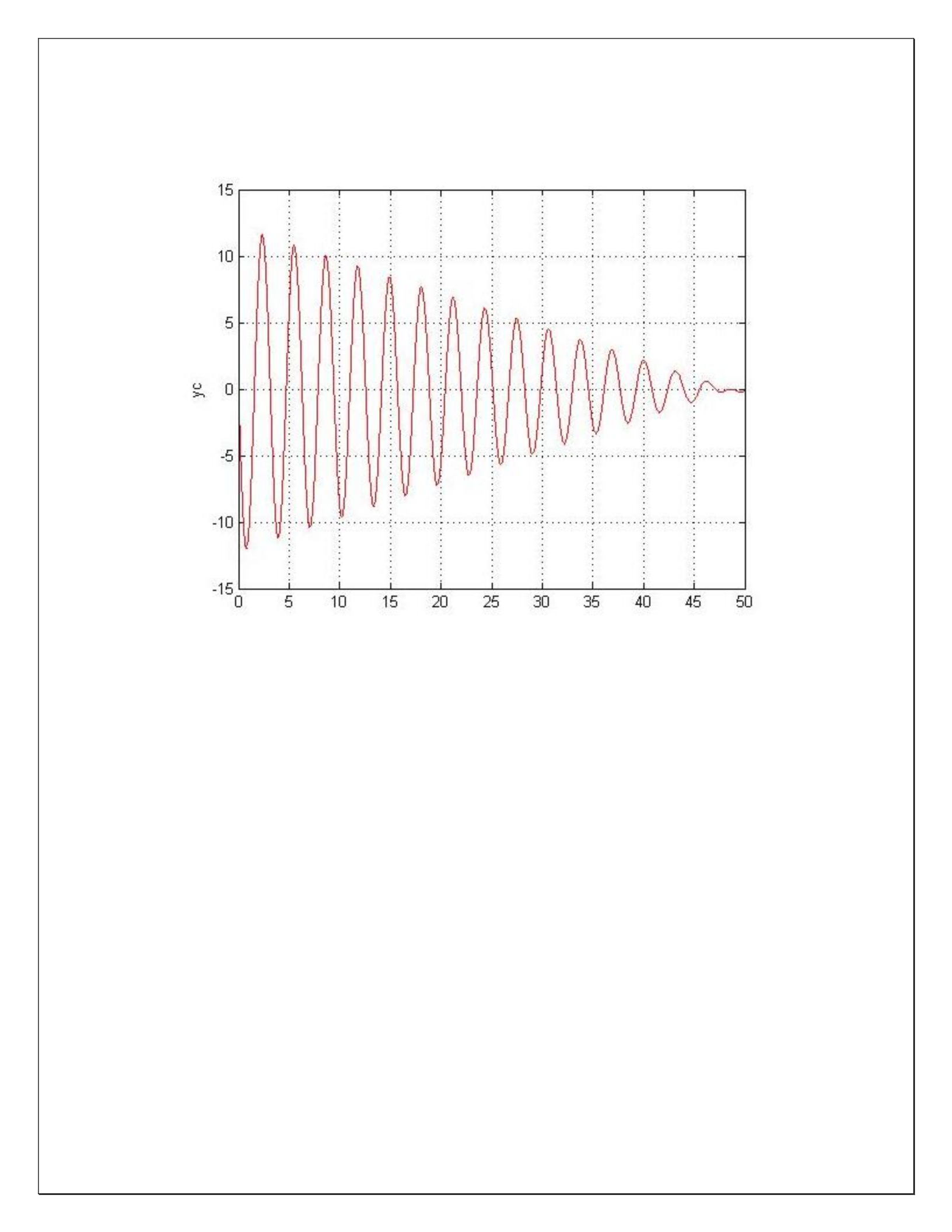
Output (B)
The following curve is obtained -
Fig 4 – Decreasing Sinusoidal
The curve resembles a typical exponentially decreasing sinusoidal wave.
% Question 4
function LAB06ex1
omega0 = 2; c = 0; omega = 1.8;
param = [omega0,c,omega];
t0 = 0; y0 = 0; v0 = 0; Y0 = [y0;v0]; tf = 100;
alpha = atan(omega/(omega0^2 - omega^2)); % Defining angle alpha here
options = odeset('AbsTol',1e-10,'RelTol',1e-10);
[t,Y] = ode45(@f,[t0,tf],Y0,options,param);
y = Y(:,1); v = Y(:,2);
% Obtaining “C” using an if criteria
if omega > omega0
C = 1/(omega^2 - omega0^2);
else
C = 1/(omega0^2 - omega^2);
end
A = 2*C * sin(0.5*(omega0 - omega).*t); % Defining the envelope function A
figure(1)
plot(t,y,'b-', t, A, 'r', t, -A, 'g'); ylabel('y'); grid on;
t1 = 25; i = find(t>t1);
C = (max(Y(i,1))-min(Y(i,1)))/2;
%yc = y - C.*cos(omega.*t - alpha); % Don’t need the complimentary solns
%figure(2)
%plot(t,yc,'r-'); ylabel('yc'); grid on;
disp(['computed amplitude of forced oscillation = ' num2str(C)]);

Ctheory = 1/sqrt((omega0^2-omega^2)^2+(c*omega)^2);
disp(['theoretical amplitude = ' num2str(Ctheory)]);
%----------------------------------------------------------------
function dYdt = f(t,Y,param)
y = Y(1); v = Y(2);
omega0 = param(1); c = param(2); omega = param(3);
dYdt = [ v ; cos(omega*t)-omega0^2*y-c*v ];
% Output (A)
Fig 5 – Envelope
% Output (B)
As per the definition the period of the fast oscillations is equal to:
T = 4π/ (ω + ωo) ωo = 2 & ω = 1.8 rad/s
T = 3.30s
The same T is obtained from the graphs as well as shown below:

Fig 6 – Time Period (1)
Fig 7 – Time Period (2)

The time period is calculated as: 9.922 – 6.614 = 3.30s
% Output (C)
The length of the beat is equal to:
L = 2π/ (ωo - ω) ωo = 2 & ω = 1.8 rad/s
L = 31.41
From the graph a similar value is obtained as shown below:
Fig 8 – Beat Length
% Output (D)
Changing value of Omega to 1.9:

Fig 9 – Omega = 1.9
Time period of the beats: 3.22s
Length of the beats: 62.83
Changing the value of omega to 1.6 rad/s

Fig 10 – Omega = 1.6
Time period of the beats: 3.5s
Length of the beats: 15.7
As the value of omega gets closer to the value of Omega0, the time period decreases as
compared to the earlier value of omega (1.8 rad/s). But there is a considerable increase in the
length of the beats as the value of omega approaches Omega0.
When we decrease the value of omega and take it further away from Omega0, the time period
increases as compared to the earlier value of omega (1.8 rad/s). But the length of the beats
decreases by a considerable amount.
% Output (E)
At Omega = 0.5 the phenomenon of the beats will not be observed. The basic criteria for having
a very rapidly varying function and a slowly varying function leads to the phenomenon of beats.
This happens when the value of Omega is close to the value of Omega0. The given value of
Omega (=0.5) is quite far from Omega0 and thus, beats will not be observed for this value of
Omega.
************THE END*************

