


%% Lab 5 – Fenil Patel - MAT 275 Lab
% The Mass-Spring System
%% EX 1
%% A)
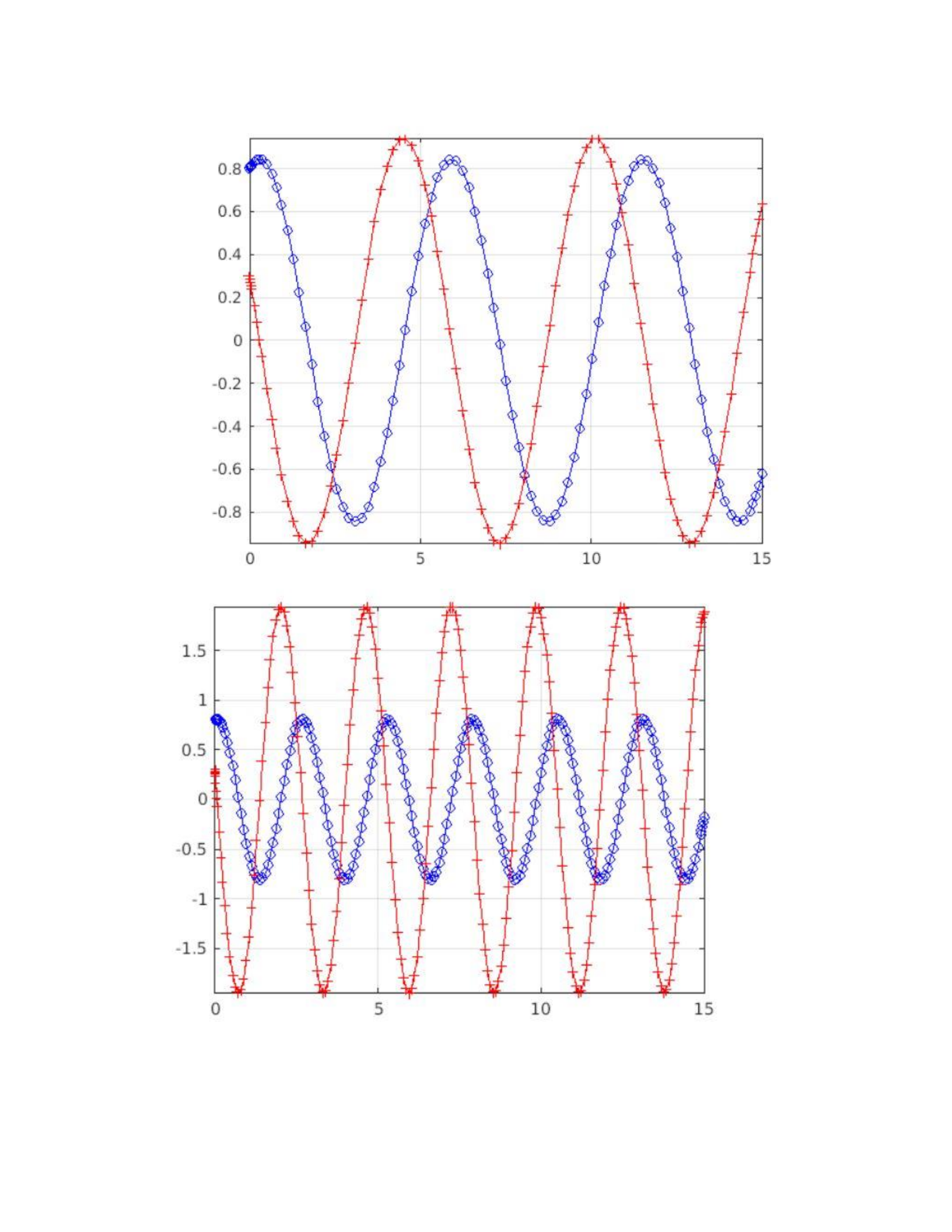
% The red curve represents y =y(t) as the red curve starts at (0,0) which
% satisfies the condition for simple harmonic motion.
%% B)
% The time period of the motion graphically is 3.91.
%- Using w0.
% T = 2*pi/w
% = 2*3.14/(5/3)
% = 3.77
%% C)
% The mass come to rest at the maximum height as the kinetic energy will be
converted to potential energy at that point and thus the position of mass remains
within an arbitrary small distance from the equilibrium point.
%% D)
% The amplitude of the graph is 0.8198
%% E)
% List the t values either in decimal format or as a fractions
% involving pi.
% Answer the question
% (2.914,1.363), (6.742,1.366), (10.58,1.354) , (4.879,1.364) ,
% (0.9716,1.346), (8.533,1.359),(12.47,1.352), (14.36,1.35)
%% F)
% Run LAB05ex1 with the given values of m and k. Include the two
% distinct graphs, each with y(t) and v(t) plotted.
% Comment on the results.
The angular velocity is directly proportional to k/m. So when the value of k
increases or m decreases, the angular velocity decreases.
%% EX 2
%% A)
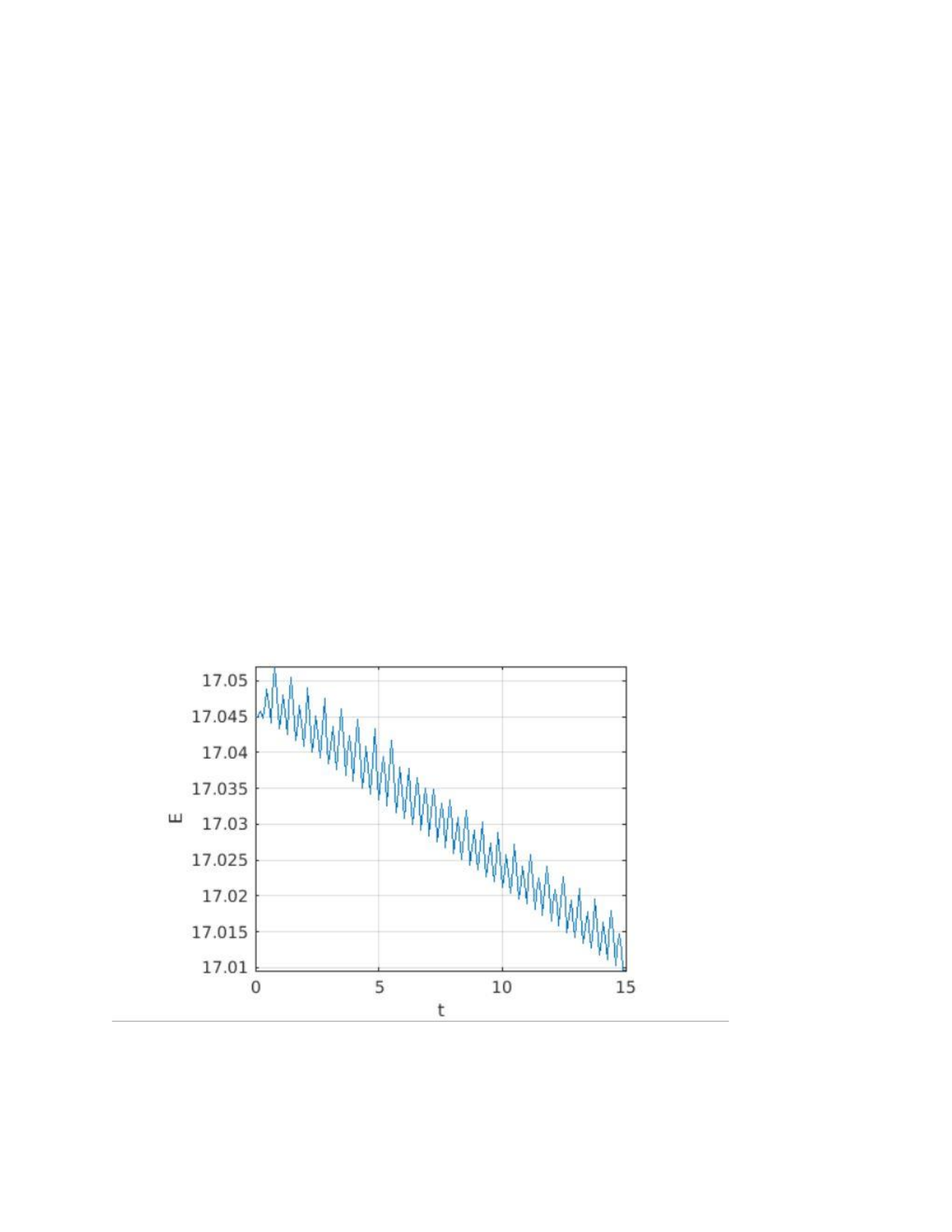
% add commands to LAB05ex1 to compute and plot E(t). Then use ylim([~,~])
% to change the yaxis limits.
% Include the code, at least one plot of E(t) and a comment.
type Lab5ex1a
Lab5ex1a
clear all; % clear all variables
m = 9; % mass [kg]
k = 25; % spring constant [N/m]
omega0 = sqrt(k/m);
y0 =0.8; v0 = 0.3; % initial conditions
[t,Y] = ode45(@f,[0,15],[y0,v0],[],omega0); % solve for 0<t<15
y = Y(:,1); v = Y(:,2); % retrieve y, v from Y
E = ((1/2.*m.*v.^2)+((1/2).*k.*y.^2));
figure(1); plot(t,y,'bo-',t,v,'r+-');% time series for y and v
figure(2);plot(t,E);
xlabel('t');
ylabel('E')
grid on; axis tight;
%---------------------------------------------------
function dYdt = f(t,Y,omega0); % function defining the DE
y = Y(1); v = Y(2);
dYdt=[ v ; - omega0^2*y ];
end
%% B)
% write out main steps here
% first differentiate E(t) with respect to t using the chain rule. Then

% make substitutions using the expression for omega0 and using the
% differential equation
% KE = 1/2*m*v^2
% PE = 1/2*k*y^2
% E = Ke + PE
% dE/dt = m*v*dv/dt + k*y*dy/dt
% = m*v*a+k*y*v (dv/dt = a , dy/dt = v)
% Since, ma = -ky
% dE/dt = -k*y*v+k*y*v
% = 0
%% c)
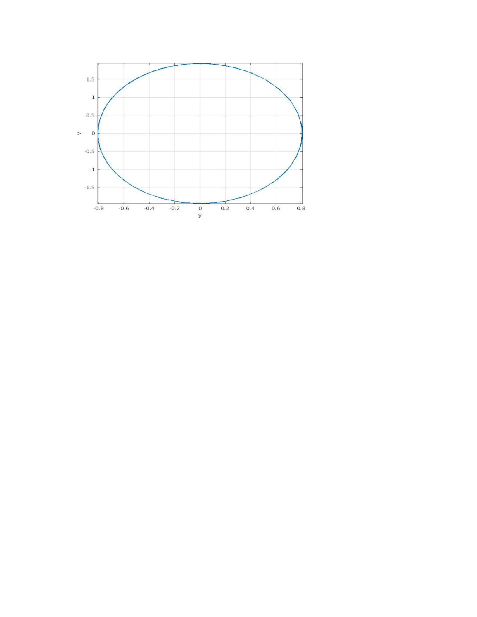
% Include modified M-file (or the added lines), plot and comment
type Lab5ex1c
Lab5ex1c
clear all; % clear all variables
m = 9; % mass [kg]
k = 52; % spring constant [N/m]
omega0 = sqrt(k/m);
y0 =0.8; v0 = 0.3; % initial conditions
[t,Y] = ode45(@f,[0,15],[y0,v0],[],omega0); % solve for 0<t<15
y = Y(:,1); v = Y(:,2); % retrieve y, v from Y
E = ((1/2.*m.*v.^2)+((1/2).*k.*y.^2));
figure(1); plot(t,y,'bo-',t,v,'r+-');% time series for y and v
figure(2);plot(t,E);
xlabel('t');
ylabel('E')
figure(3) ; plot(y,v);
xlabel('y');
ylabel('v');
grid on; axis tight;
%---------------------------------------------------
function dYdt = f(t,Y,omega0); % function defining the DE
y = Y(1); v = Y(2);
dYdt=[ v ; - omega0^2*y ];
end
%% EX 3
%% A)
% 4.596
% modify the system of equations in LAB05ex2
% write the t value. I you use the given matlab commands you will need to explain
them.
%% B)
% write t value and max |V| value;
% note: velocity magnitude is like absolute value!
% The maximum velocity attained is 0.8817 m/s at 0.8861s
%% C)
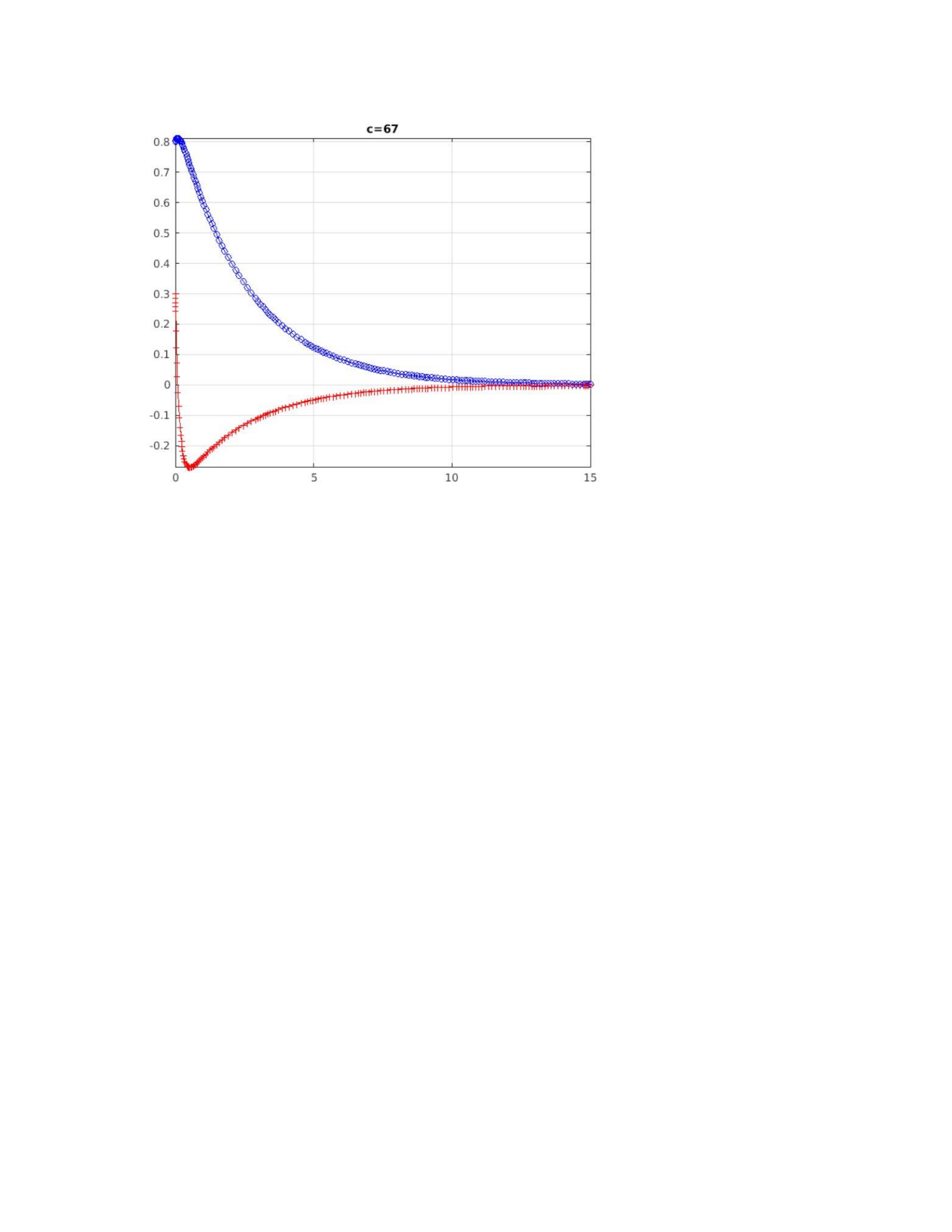
% include 3 figures here + comments.
% use title('text') to attach a title to the figure
% The resistance of the motion increases as the value of c increases
% beacuse with the higher value of c, the mass reaches the equilibrium
% position faster.

%% D)
% What needs to happen (in terms of the characteristic equation)
% in order for there to be no oscillations? Impose a condition on the
% characteristic equation to find the critical c value. Write out main steps
% The motion will be critically damped if the characteristic equation
% have repeated roots.
% Therefore, s^2 +2ps + w0^2 = 0
% Thus, 4p^2s^2-4s^2*w0^2 = 0
% p^2 = wo^2
% (c/2m)^2 = w0^2
% c = 2*m*w0
% c = 2*9*1.6667
% c = 30
%% EX4
%% A)
% include the completed M-file, 1 figure and comment
type Lab5ex2a
Lab5ex2a
clear all; % clear all variables
m = 9; % mass [kg]
k = 25; % spring constant [N/m]
c = 10; % friction coefficient [Ns/m]
omega0 = sqrt(k/m); p = c/(2*m);
y0 =0.8; v0 = 0.3; % initial conditions
[t,Y] = ode45(@f,[0,15],[y0,v0],[],omega0, p); % solve for 0<t<15
y = Y(:,1); v = Y(:,2); % retrieve y, v from Y
figure(1); plot(t,y,'bo-',t,v,'r+-');% time series for y and v
E = ((1/2.*m.*v.^2)+((1/2).*k.*y.^2));
figure(2);plot(t,E);
xlabel('t');
ylabel('E');
grid on; axis tight;
%---------------------------------------------------
function dYdt = f(t,Y,omega0,p); % function defining the DE
y = Y(1); v = Y(2);
dYdt=[ v ; -2.*p*v- omega0.^2*y ]; % fill-in dv/dt
end
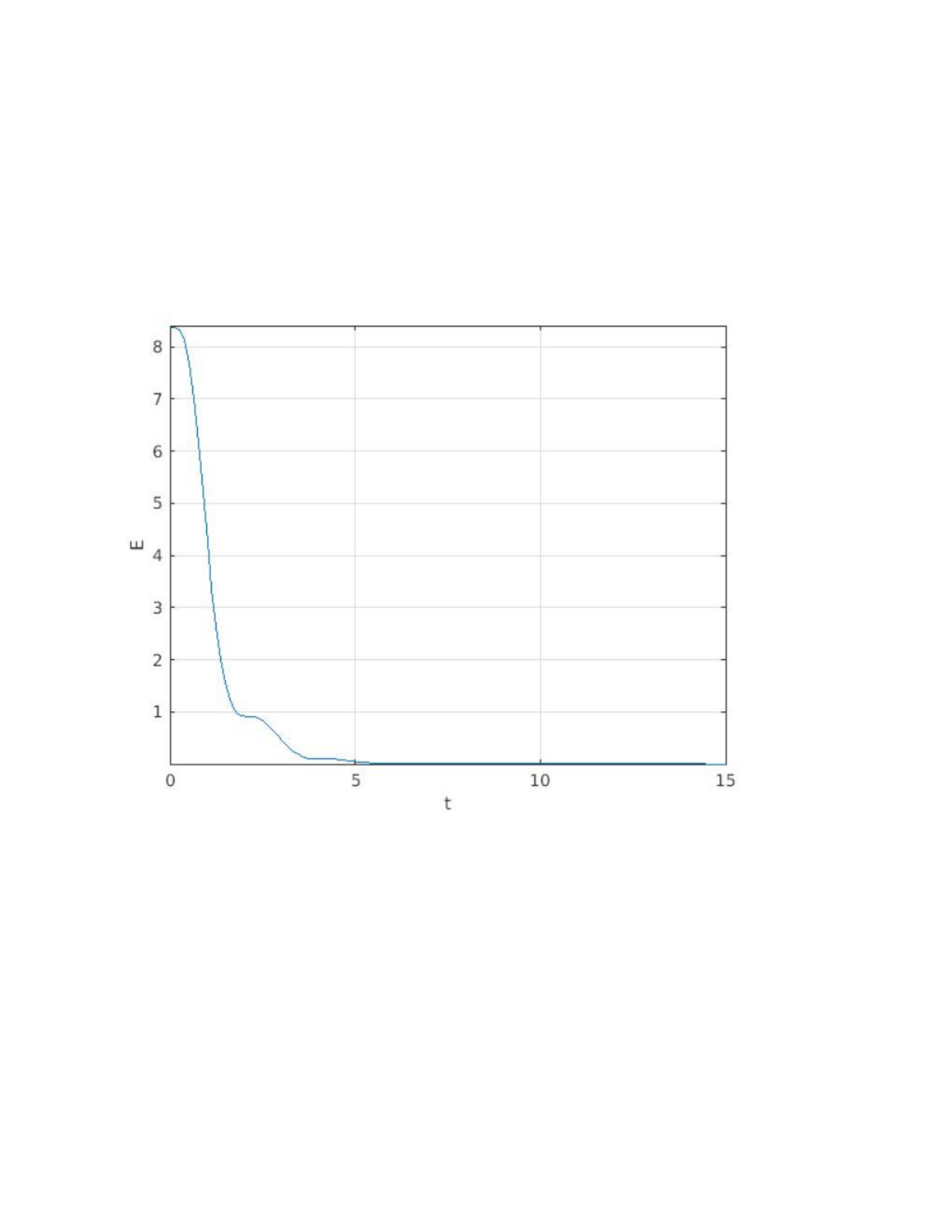
The energy is not conserved according to the plot as the energy gets to zero at t
=5 because it is damped.
%% B)
% again find dE/dt using the chain rule and make substitutions based on the
% differential equation. You should reach an expression for dE/dt which is
% in terms of y
% KE = 1/2*m*v^2
% PE = 1/2*k*y^2
% E = KE + PE
% dE/dt = m*v*dv/dt + k*y*dy/dt
% Since v = c/n and dy/dt = v
% dE/dt = (c/n) * (m*dv/dt + k*y),
% Since there is a pullinf force, (m*dv/dt + k*y) is negative
% And thus, dE/dt < 0 if c>0 & dE/dt > 0 if c<0
%
%% C)
% Include M-file (or the added lines), one figure and comment
type Lab5ex2c
Lab5ex2c
clear all; % clear all variables
m = 9; % mass [kg]
k = 25; % spring constant [N/m]
c = 10; % friction coefficient [Ns/m]
omega0 = sqrt(k/m); p = c/(2*m);
y0 =0.8; v0 = 0.3; % initial conditions
[t,Y] = ode45(@f,[0,15],[y0,v0],[],omega0, p); % solve for 0<t<15
y = Y(:,1); v = Y(:,2); % retrieve y, v from Y
figure(1); plot(t,y,'bo-',t,v,'r+-');% time series for y and v
E = ((1/2.*m.*v.^2)+((1/2).*k.*y.^2));
figure(2);plot(t,E);
xlabel('t');
ylabel('E')
figure(3) ; plot(y,v);
xlabel('y');
ylabel('v');
grid on; axis tight;
%---------------------------------------------------
function dYdt = f(t,Y,omega0,p); % function defining the DE
y = Y(1); v = Y(2);
dYdt=[ v ; -2.*p*v- omega0.^2*y ]; % fill-in dv/dt
end
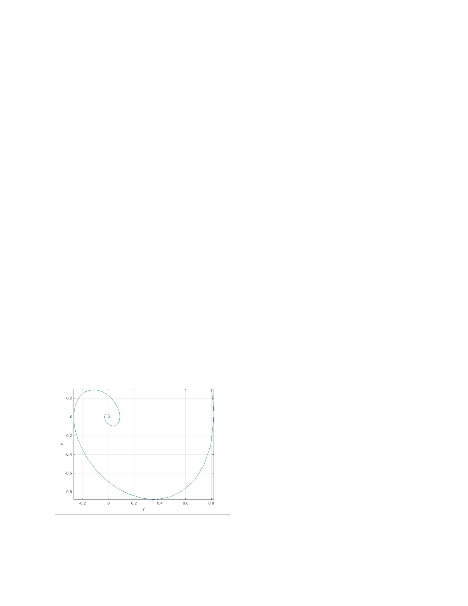
The curve gets closer to the origin as the phase plot ends at 0,0. Since the
system is damped, the total energy is not conserved. The curve seems to have
spiral behavior.


