


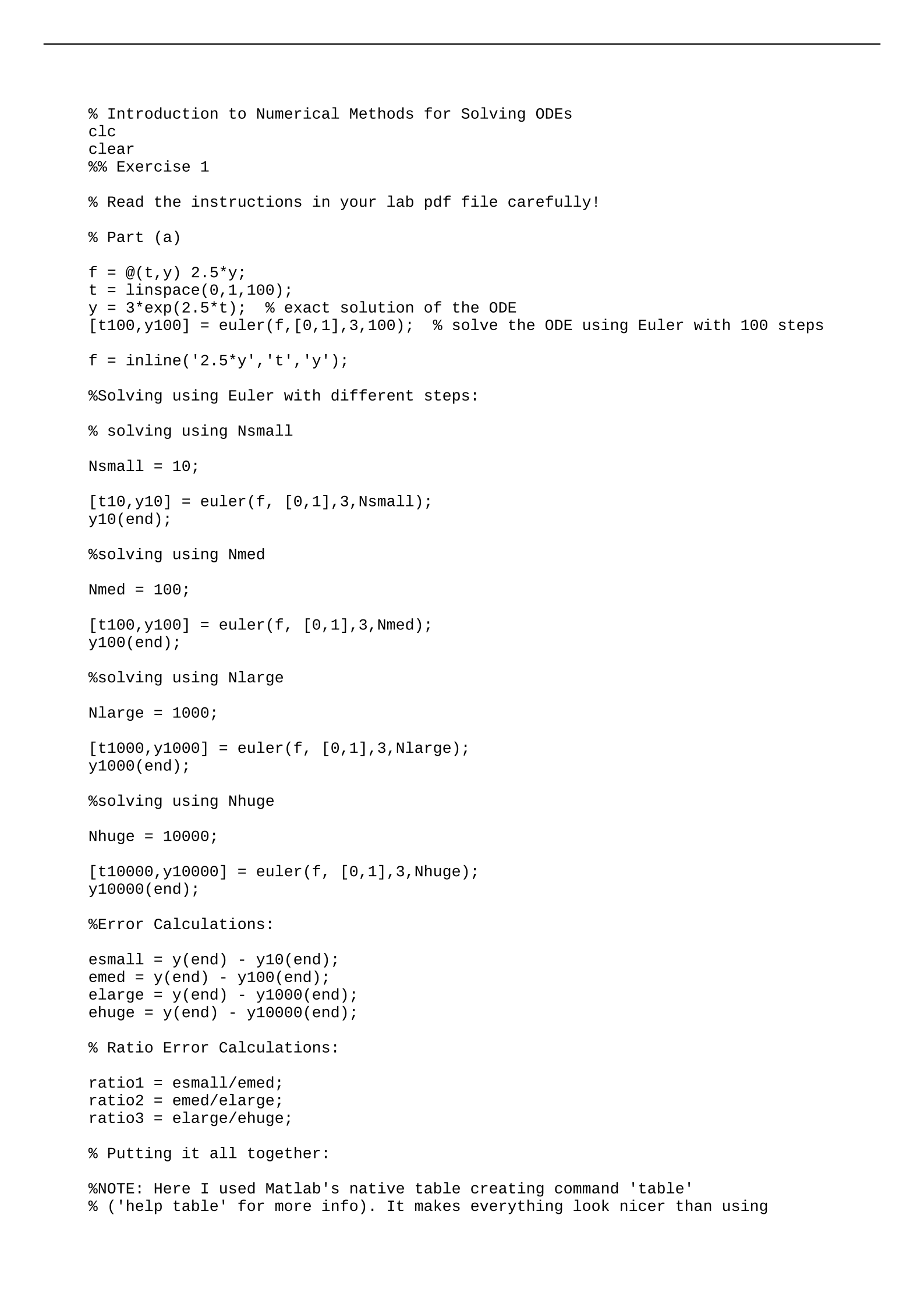
% Introduction to Numerical Methods for Solving ODEs
clc
clear
%% Exercise 1
% Read the instructions in your lab pdf file carefully!
% Part (a)
f = @(t,y) 2.5*y;
t = linspace(0,1,100);
y = 3*exp(2.5*t); % exact solution of the ODE
[t100,y100] = euler(f,[0,1],3,100); % solve the ODE using Euler with 100 steps
f = inline('2.5*y','t','y');
%Solving using Euler with different steps:
% solving using Nsmall
Nsmall = 10;
[t10,y10] = euler(f, [0,1],3,Nsmall);
y10(end);
%solving using Nmed
Nmed = 100;
[t100,y100] = euler(f, [0,1],3,Nmed);
y100(end);
%solving using Nlarge
Nlarge = 1000;
[t1000,y1000] = euler(f, [0,1],3,Nlarge);
y1000(end);
%solving using Nhuge
Nhuge = 10000;
[t10000,y10000] = euler(f, [0,1],3,Nhuge);
y10000(end);
%Error Calculations:
esmall = y(end) - y10(end);
emed = y(end) - y100(end);
elarge = y(end) - y1000(end);
ehuge = y(end) - y10000(end);
% Ratio Error Calculations:
ratio1 = esmall/emed;
ratio2 = emed/elarge;
ratio3 = elarge/ehuge;
% Putting it all together:
%NOTE: Here I used Matlab's native table creating command 'table'
% ('help table' for more info). It makes everything look nicer than using
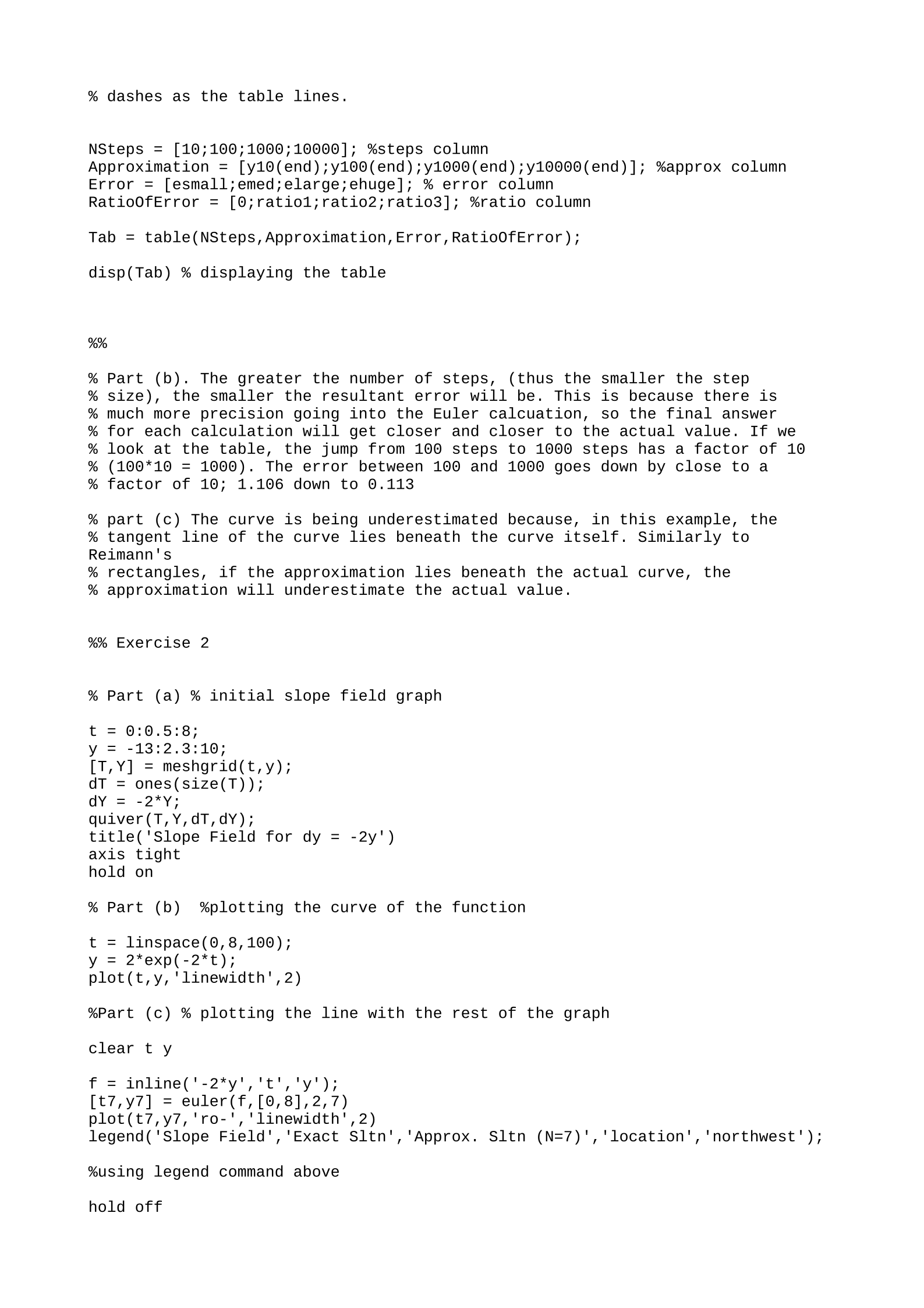
% dashes as the table lines.
NSteps = [10;100;1000;10000]; %steps column
Approximation = [y10(end);y100(end);y1000(end);y10000(end)]; %approx column
Error = [esmall;emed;elarge;ehuge]; % error column
RatioOfError = [0;ratio1;ratio2;ratio3]; %ratio column
Tab = table(NSteps,Approximation,Error,RatioOfError);
disp(Tab) % displaying the table
%%
% Part (b). The greater the number of steps, (thus the smaller the step
% size), the smaller the resultant error will be. This is because there is
% much more precision going into the Euler calcuation, so the final answer
% for each calculation will get closer and closer to the actual value. If we
% look at the table, the jump from 100 steps to 1000 steps has a factor of 10
% (100*10 = 1000). The error between 100 and 1000 goes down by close to a
% factor of 10; 1.106 down to 0.113
% part (c) The curve is being underestimated because, in this example, the
% tangent line of the curve lies beneath the curve itself. Similarly to
Reimann's
% rectangles, if the approximation lies beneath the actual curve, the
% approximation will underestimate the actual value.
%% Exercise 2
% Part (a) % initial slope field graph
t = 0:0.5:8;
y = -13:2.3:10;
[T,Y] = meshgrid(t,y);
dT = ones(size(T));
dY = -2*Y;
quiver(T,Y,dT,dY);
title('Slope Field for dy = -2y')
axis tight
hold on
% Part (b) %plotting the curve of the function
t = linspace(0,8,100);
y = 2*exp(-2*t);
plot(t,y,'linewidth',2)
%Part (c) % plotting the line with the rest of the graph
clear t y
f = inline('-2*y','t','y');
[t7,y7] = euler(f,[0,8],2,7)
plot(t7,y7,'ro-','linewidth',2)
legend('Slope Field','Exact Sltn','Approx. Sltn (N=7)','location','northwest');
%using legend command above
hold off
%%
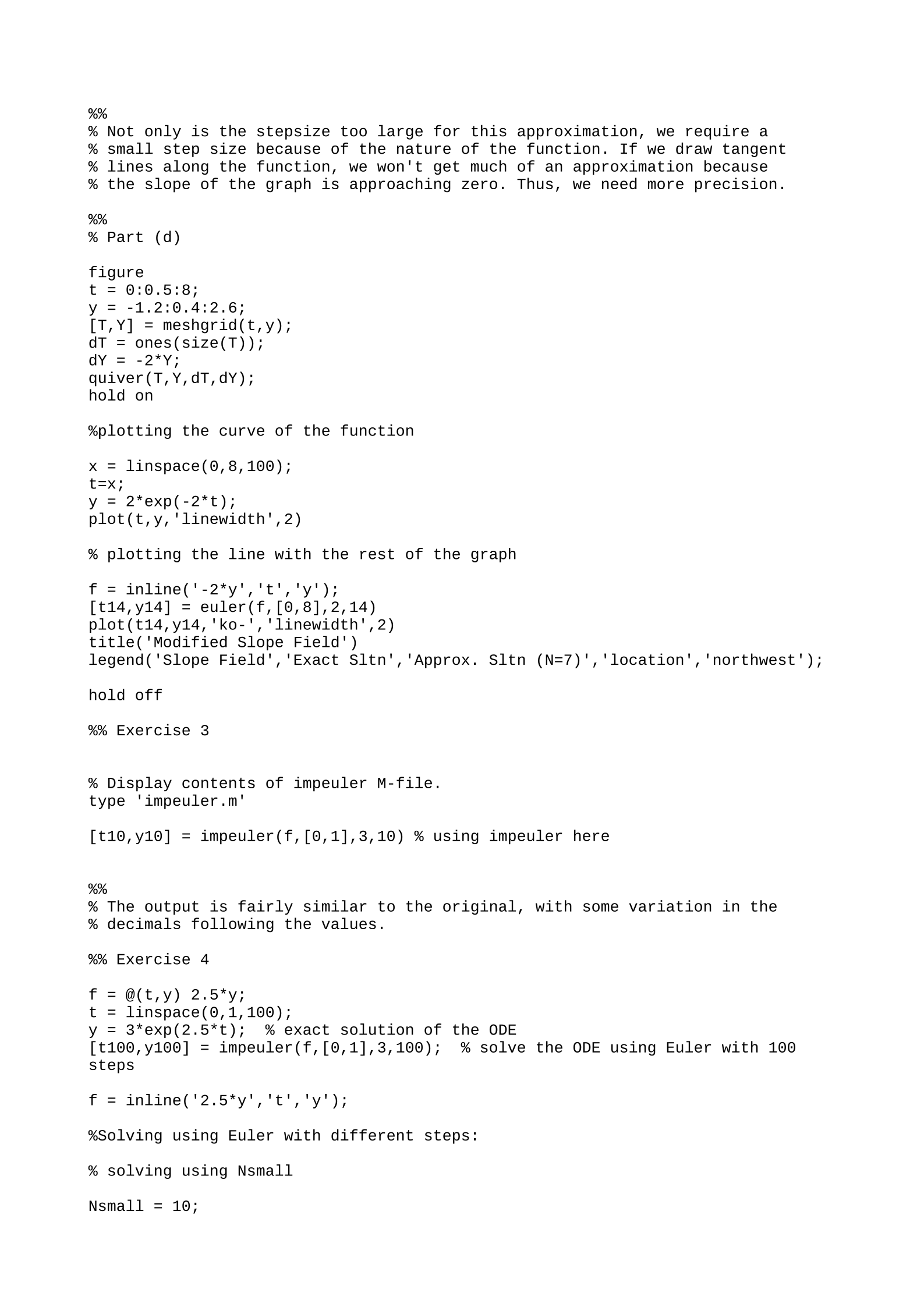
% Not only is the stepsize too large for this approximation, we require a
% small step size because of the nature of the function. If we draw tangent
% lines along the function, we won't get much of an approximation because
% the slope of the graph is approaching zero. Thus, we need more precision.
%%
% Part (d)
figure
t = 0:0.5:8;
y = -1.2:0.4:2.6;
[T,Y] = meshgrid(t,y);
dT = ones(size(T));
dY = -2*Y;
quiver(T,Y,dT,dY);
hold on
%plotting the curve of the function
x = linspace(0,8,100);
t=x;
y = 2*exp(-2*t);
plot(t,y,'linewidth',2)
% plotting the line with the rest of the graph
f = inline('-2*y','t','y');
[t14,y14] = euler(f,[0,8],2,14)
plot(t14,y14,'ko-','linewidth',2)
title('Modified Slope Field')
legend('Slope Field','Exact Sltn','Approx. Sltn (N=7)','location','northwest');
hold off
%% Exercise 3
% Display contents of impeuler M-file.
type 'impeuler.m'
[t10,y10] = impeuler(f,[0,1],3,10) % using impeuler here
%%
% The output is fairly similar to the original, with some variation in the
% decimals following the values.
%% Exercise 4
f = @(t,y) 2.5*y;
t = linspace(0,1,100);
y = 3*exp(2.5*t); % exact solution of the ODE
[t100,y100] = impeuler(f,[0,1],3,100); % solve the ODE using Euler with 100
steps
f = inline('2.5*y','t','y');
%Solving using Euler with different steps:
% solving using Nsmall
Nsmall = 10;
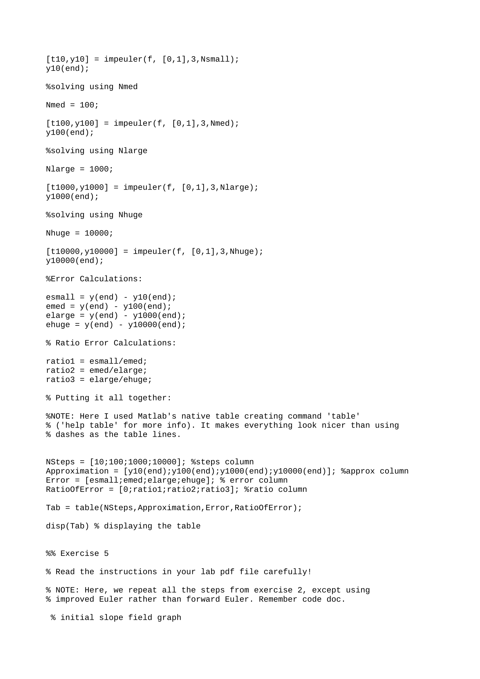
[t10,y10] = impeuler(f, [0,1],3,Nsmall);
y10(end);
%solving using Nmed
Nmed = 100;
[t100,y100] = impeuler(f, [0,1],3,Nmed);
y100(end);
%solving using Nlarge
Nlarge = 1000;
[t1000,y1000] = impeuler(f, [0,1],3,Nlarge);
y1000(end);
%solving using Nhuge
Nhuge = 10000;
[t10000,y10000] = impeuler(f, [0,1],3,Nhuge);
y10000(end);
%Error Calculations:
esmall = y(end) - y10(end);
emed = y(end) - y100(end);
elarge = y(end) - y1000(end);
ehuge = y(end) - y10000(end);
% Ratio Error Calculations:
ratio1 = esmall/emed;
ratio2 = emed/elarge;
ratio3 = elarge/ehuge;
% Putting it all together:
%NOTE: Here I used Matlab's native table creating command 'table'
% ('help table' for more info). It makes everything look nicer than using
% dashes as the table lines.
NSteps = [10;100;1000;10000]; %steps column
Approximation = [y10(end);y100(end);y1000(end);y10000(end)]; %approx column
Error = [esmall;emed;elarge;ehuge]; % error column
RatioOfError = [0;ratio1;ratio2;ratio3]; %ratio column
Tab = table(NSteps,Approximation,Error,RatioOfError);
disp(Tab) % displaying the table
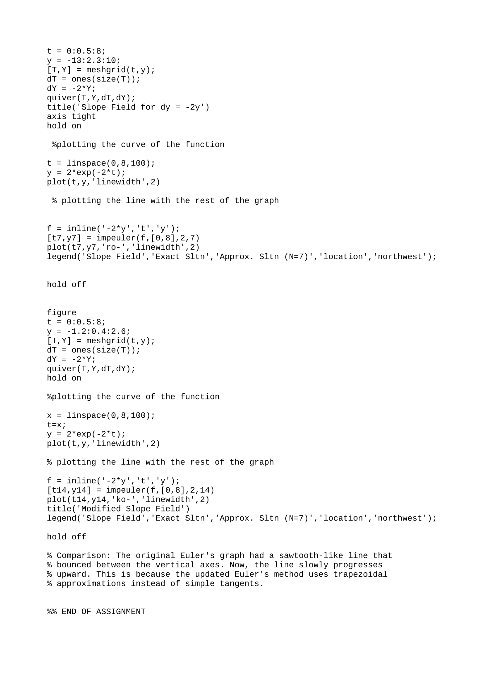
%% Exercise 5
% Read the instructions in your lab pdf file carefully!
% NOTE: Here, we repeat all the steps from exercise 2, except using
% improved Euler rather than forward Euler. Remember code doc.
% initial slope field graph
t = 0:0.5:8;
y = -13:2.3:10;
[T,Y] = meshgrid(t,y);
dT = ones(size(T));
dY = -2*Y;
quiver(T,Y,dT,dY);
title('Slope Field for dy = -2y')
axis tight
hold on
%plotting the curve of the function
t = linspace(0,8,100);
y = 2*exp(-2*t);
plot(t,y,'linewidth',2)
% plotting the line with the rest of the graph
f = inline('-2*y','t','y');
[t7,y7] = impeuler(f,[0,8],2,7)
plot(t7,y7,'ro-','linewidth',2)
legend('Slope Field','Exact Sltn','Approx. Sltn (N=7)','location','northwest');
hold off
figure
t = 0:0.5:8;
y = -1.2:0.4:2.6;
[T,Y] = meshgrid(t,y);
dT = ones(size(T));
dY = -2*Y;
quiver(T,Y,dT,dY);
hold on
%plotting the curve of the function
x = linspace(0,8,100);
t=x;
y = 2*exp(-2*t);
plot(t,y,'linewidth',2)
% plotting the line with the rest of the graph
f = inline('-2*y','t','y');
[t14,y14] = impeuler(f,[0,8],2,14)
plot(t14,y14,'ko-','linewidth',2)
title('Modified Slope Field')
legend('Slope Field','Exact Sltn','Approx. Sltn (N=7)','location','northwest');
hold off
% Comparison: The original Euler's graph had a sawtooth-like line that
% bounced between the vertical axes. Now, the line slowly progresses
% upward. This is because the updated Euler's method uses trapezoidal
% approximations instead of simple tangents.
%% END OF ASSIGNMENT
Powered by TCPDF (www.tcpdf.org)

