


Thomas Lashua MATLAB LAB 5
% MAT 275 MATLAB ASSIGNMENT #5
%Exercise #1
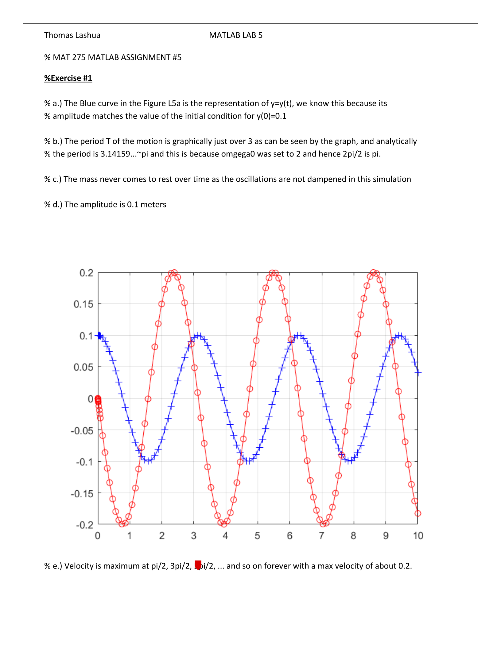
% a.) The Blue curve in the Figure L5a is the representation of y=y(t), we know this because its
% amplitude matches the value of the initial condition for y(0)=0.1
% b.) The period T of the motion is graphically just over 3 as can be seen by the graph, and analytically
% the period is 3.14159...~pi and this is because omgega0 was set to 2 and hence 2pi/2 is pi.
% c.) The mass never comes to rest over time as the oscillations are not dampened in this simulation
% d.) The amplitude is 0.1 meters
% e.) Velocity is maximum at pi/2, 3pi/2, 5pi/2, ... and so on forever with a max velocity of about 0.2.
Thomas Lashua MATLAB LAB 5 November 20, 2016
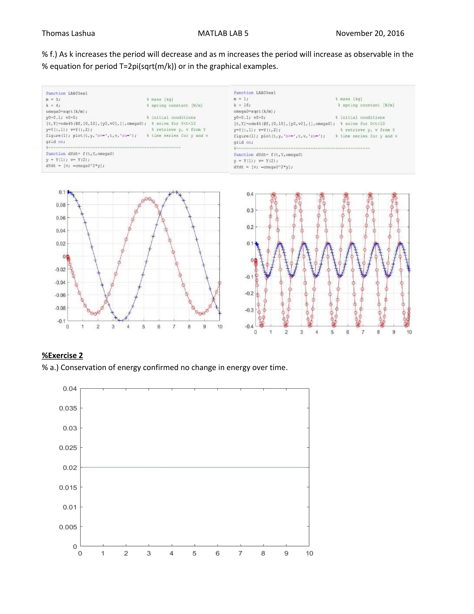
% f.) As k increases the period will decrease and as m increases the period will increase as observable in the
% equation for period T=2pi(sqrt(m/k)) or in the graphical examples.
%Exercise 2
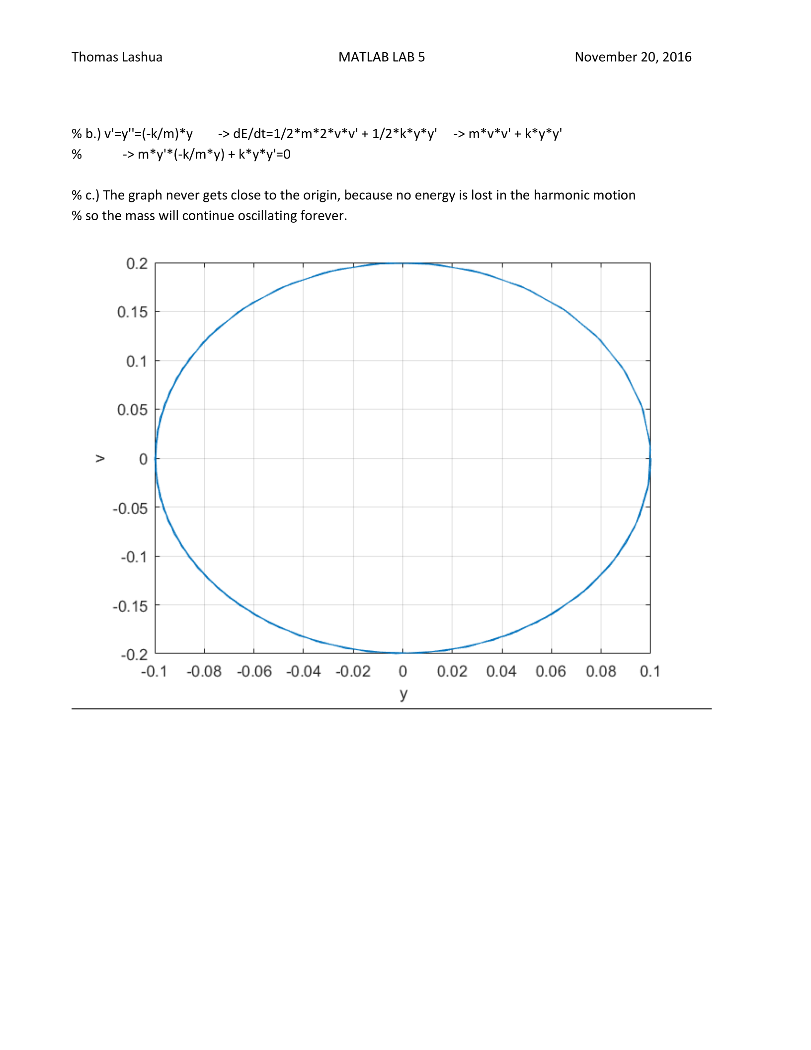
% a.) Conservation of energy confirmed no change in energy over time.
Thomas Lashua MATLAB LAB 5 November 20, 2016
% b.) v'=y''=(-k/m)*y -> dE/dt=1/2*m*2*v*v' + 1/2*k*y*y' -> m*v*v' + k*y*y'
% -> m*y'*(-k/m*y) + k*y*y'=0
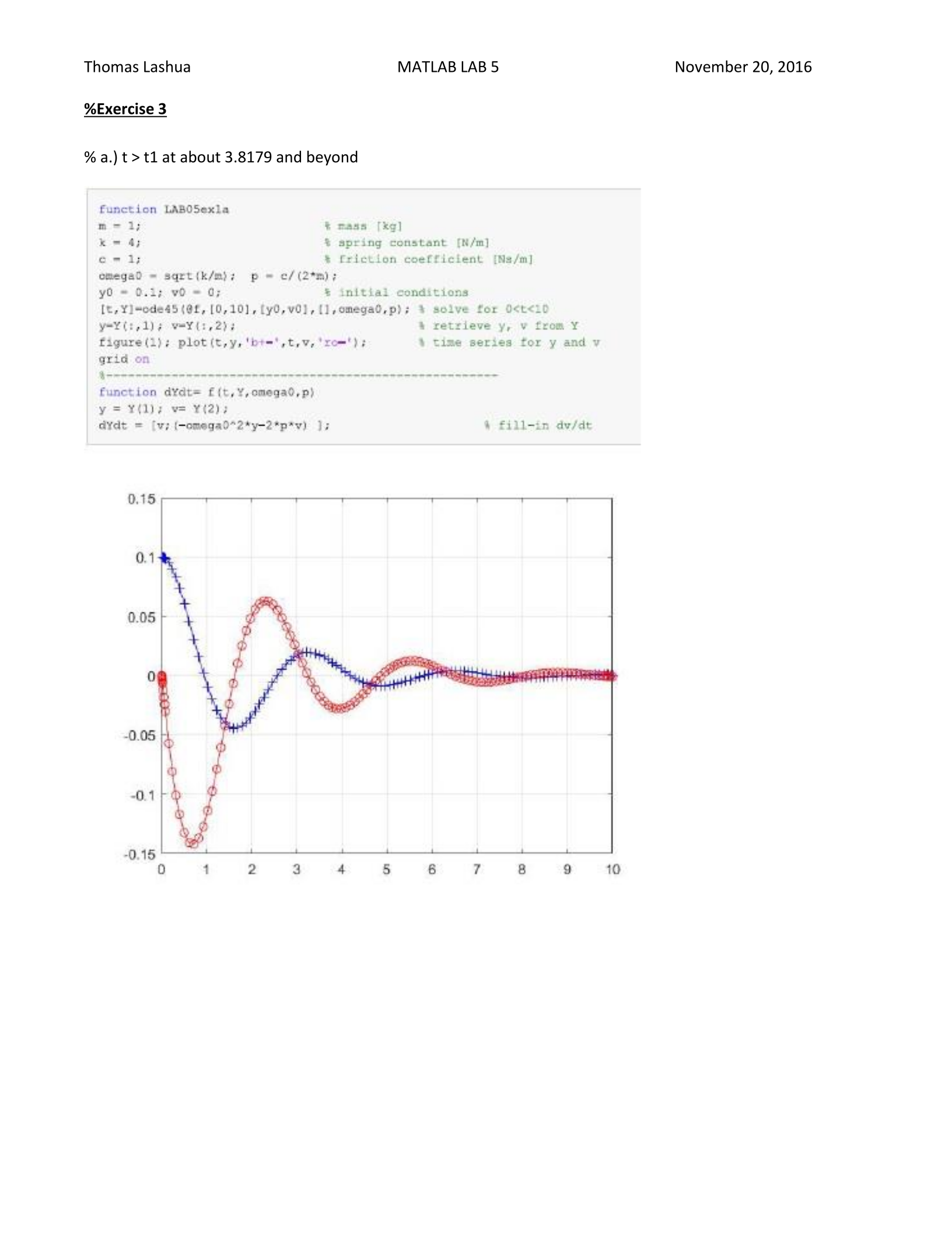
% c.) The graph never gets close to the origin, because no energy is lost in the harmonic motion
% so the mass will continue oscillating forever.
function
LABOSexla
m=
i;
&
mass
[Xq]
k=
4; %
spring
constant
[N/m]
cw
il;
&
friction
coefficient
[Ns/m]
omegad
=
sqrt(k/m);
p
=
c/(2*m);
yO
=
0.3;
vO =
0;
©
initial
conditions
[t,
¥]“ode45(@f,
[0,10],
(y0,v0},{],omegad,p);
%
solve
for
O<t<10
yey(r,l)¢
wey:,2)3
&
retrieve
y,
v
from
Y
figure(l);
plot(t,y,'bt=',t,v,
rom");
%
time
series
for
y
and
v
grid
on
4
function
d¥dt=
f(t,
¥,omega0,p)
y =
¥(1l);
w=
¥(2);2
adydt
=
[v;
(-omega0*2*y-2*p*v)
Jj;
&
fill-in
dv/dt
Thomas Lashua MATLAB LAB 5 November 20, 2016
%Exercise 3
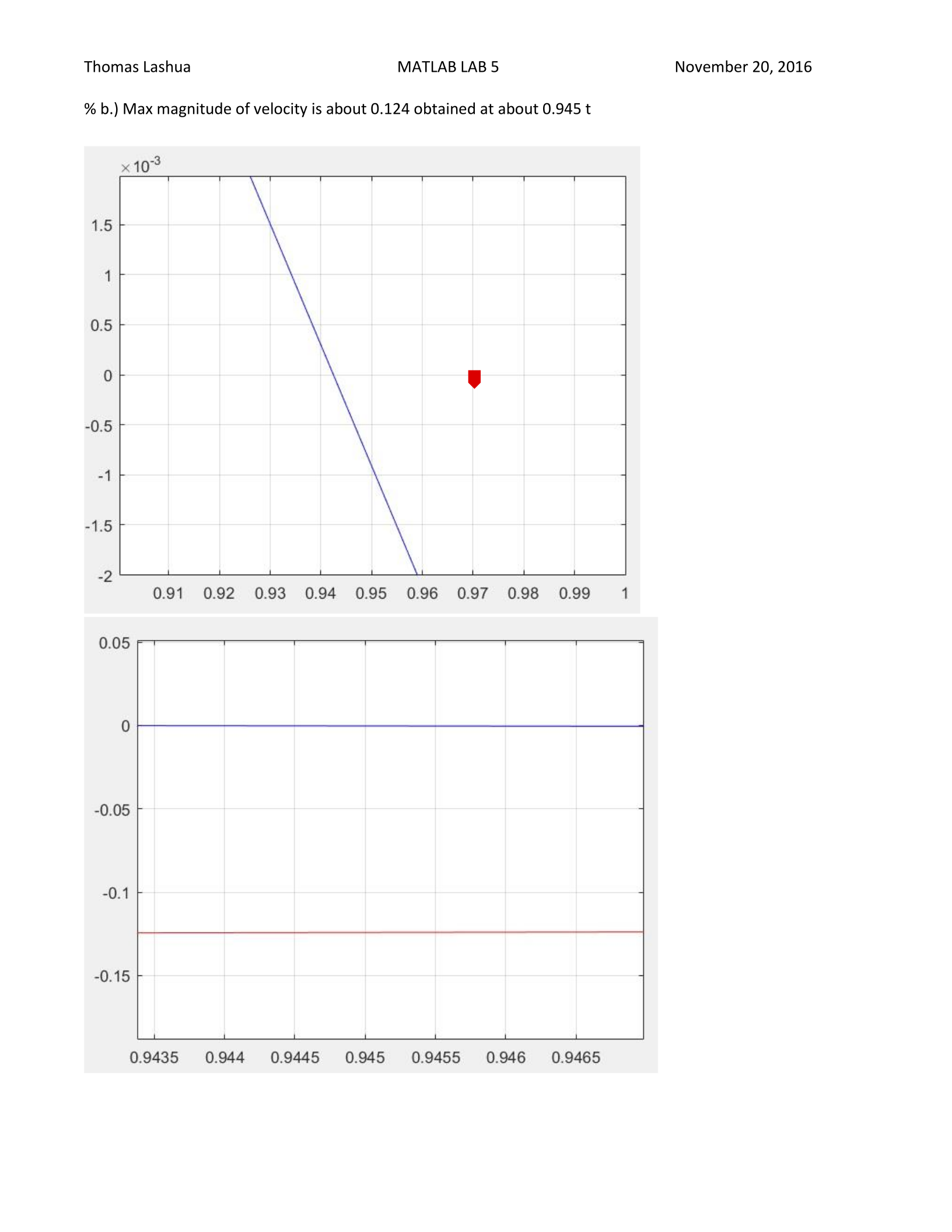
% a.) t > t1 at about 3.8179 and beyond
1.5
5
0.5
pe
i
1
i i 1
0.91
092 093 094 095 096
0.97 0.98 0.99
0.05
]
|
|
|
-0.05
fF
-0.15
iii
i i i
0.9435
0.944
0.9445
0.945
0.9455
0.946
0.9465
Thomas Lashua MATLAB LAB 5 November 20, 2016
% b.) Max magnitude of velocity is about 0.124 obtained at about 0.945 t

0.15
0.14%
0.05
10
0.08
0.06
0.04
0.02
10
Thomas Lashua MATLAB LAB 5 November 20, 2016
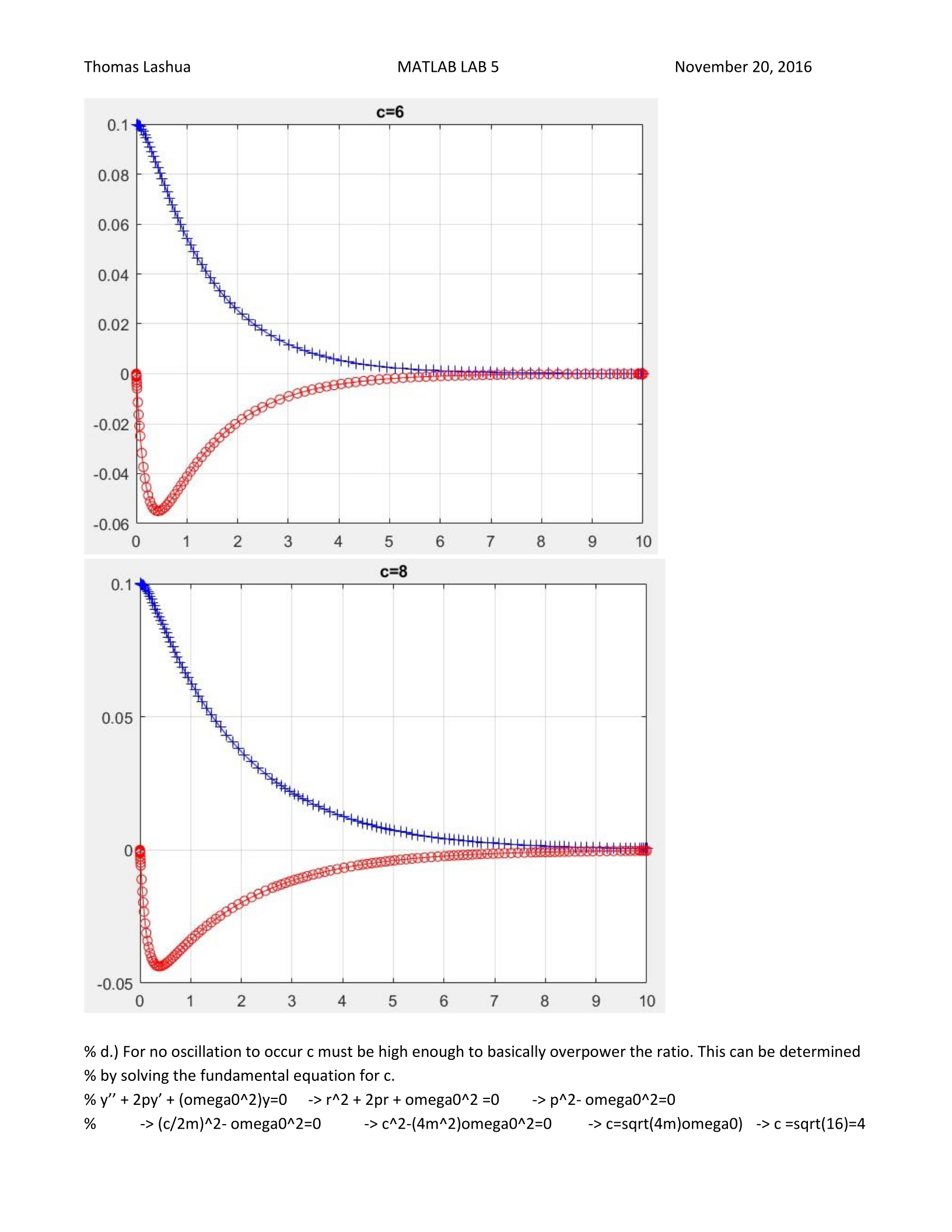
% c.) The c value will change how much the motion is damped as it goes higher the more dampened the motion
% becomes going from underdamped to overdamped in these examples with critical dampening at about c=4
Thomas Lashua MATLAB LAB 5 November 20, 2016
% d.) For no oscillation to occur c must be high enough to basically overpower the ratio. This can be determined
% by solving the fundamental equation for c.
% y’’ + 2py’ + (omega0^2)y=0 -> r^2 + 2pr + omega0^2 =0 -> p^2- omega0^2=0
% -> (c/2m)^2- omega0^2=0 -> c^2-(4m^2)omega0^2=0 -> c=sqrt(4m)omega0) -> c =sqrt(16)=4
Thomas Lashua MATLAB LAB 5 November 20, 2016
% Exercise 4
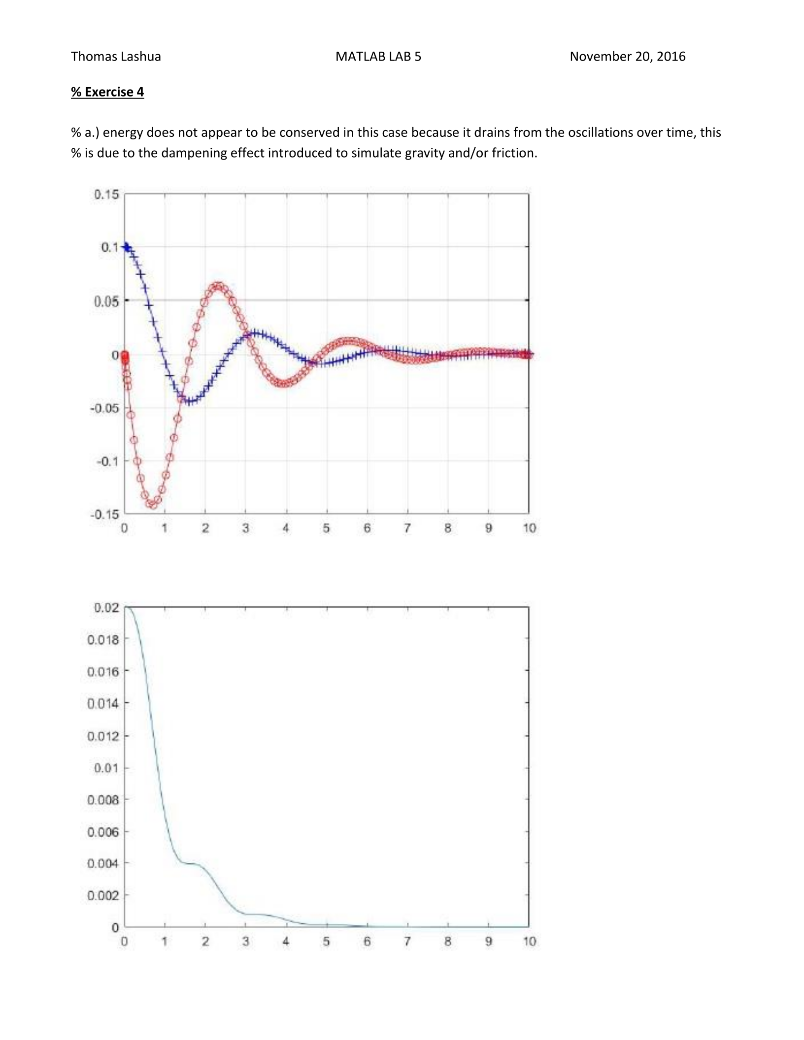
% a.) energy does not appear to be conserved in this case because it drains from the oscillations over time, this
% is due to the dampening effect introduced to simulate gravity and/or friction.
Thomas Lashua MATLAB LAB 5 November 20, 2016
% b.) v'=y''=(-k/m)*y -> dE/dt=1/2*m*2*v*v' + 1/2*k*y*y'-c -> m*v*v' + k*y*y'-c*t
% -> m*y'*(-k/m)*y + k*y*y'-c*t =0 -> ( -k *y* y' + k*y*y')/t =c
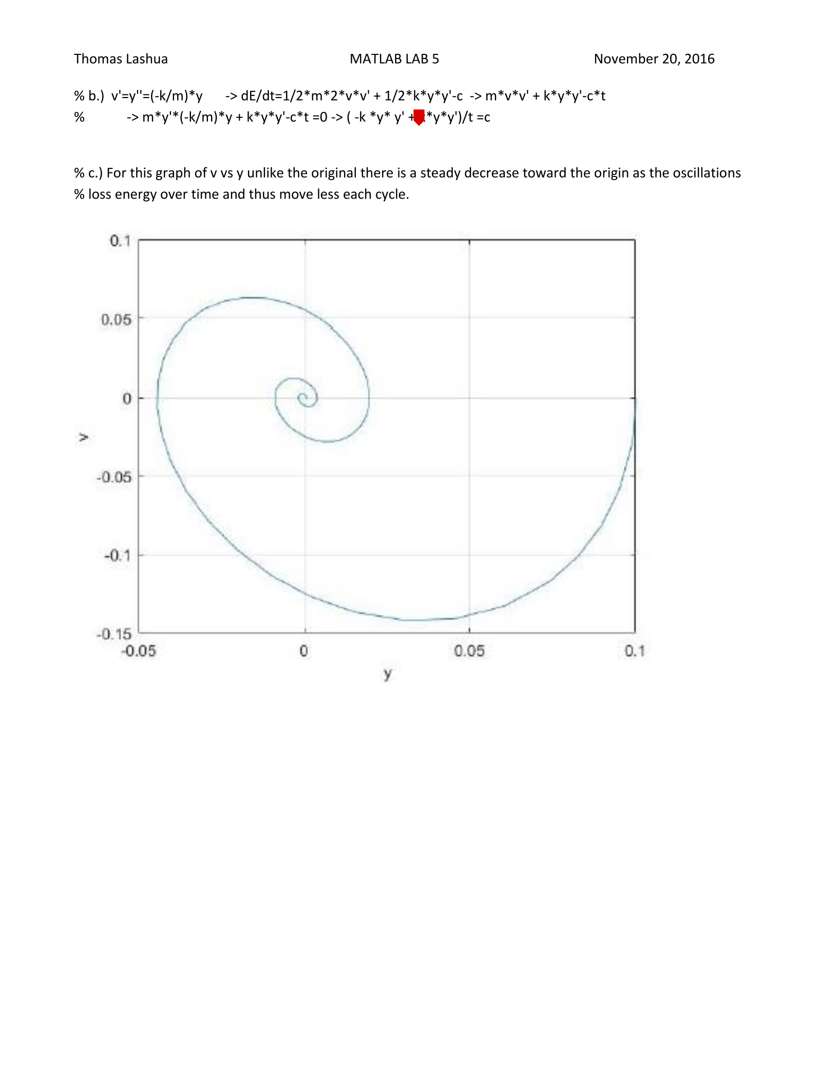
% c.) For this graph of v vs y unlike the original there is a steady decrease toward the origin as the oscillations
% loss energy over time and thus move less each cycle.
Powered by TCPDF (www.tcpdf.org)

