


1
Chapter 1: Introduction to the Study
Background of the BIED GPM Study
During the December 8, 2001 Nobel Prize lecture titled “Information and the
Change in the Paradigm in Economics,” Nobel Laureate Stiglitz (2001) stated, “When I
began the study of economics some forty one years ago, I was struck by the incongruity
between the models that I was taught and the world that I had seen growing up”(para. 4)
Nobel Laureate Ostrom (2009) announced on the same day 8 years later in her Nobel
Prize lecture titled “Beyond Markets and States: Polycentric Governance of Complex
Economic Systems” that “we need to develop a better theoretical understanding of human
behavior as well as of the impact of the diverse contexts that humans face”(para. 91).
Ostrom went on to say, “We should continue to use simple models where they capture
enough of the core underlying structure and incentives that they usefully predict
outcomes” (para. 91).
Stiglitz and Ostrom are reputed as two of the brightest minds in the world of
economics. They defined and prescribed two specific problems and call for new
solutions. The first problem is one of applicable and efficient economic models. There is
a need for as simple a model as possible that may help shape the understanding of events
seen today and be used as a tool to promote an understanding of tomorrow’s economic
events (Stiglitz, 2001). Ostrom, the first woman to receive the Nobel Prize in Economics,
identified the second problem, which is the need to include behavior in modern
development research (Ostrom, 2009).

2
The limit to economic models and the absence of human behavior indicators has
been identified. This gap is addressed in this study. This research focuses on the more
specific sub discipline of economic growth known as development economics.
Specifically, their research addressed the question of whether the same problem exists in
development economics. Kooros and Badeaux (2007) further address this gap in the
literature when they identify in their research the absence of extensive economic
development models in the broader academic spectrum. The repeated acknowledgement
that there is a gap in the literature both in economics and in the sub discipline of
development economics suggests that a new model may be needed to further contribute
to the understanding of such complex economic and development issues. Human
behavior should be included as a new indicator in this developing model to depict the
contribution of labor in economic growth. This new model with a behavioral indicator
adds to the growing body of research known as behavioral economics.
Problem Statement
A problem in economics has been identified: Stiglitz (2001) encouraged new
models in economics as a discipline, Ostrom (2009) encourages the addition of behavior
indicators in new models, and Kooros and Badeaux (2007) encourage new models
specifically in development economics. If economics can benefit from a tighter
relationship between development economics and behavior economics, then creation of a
new model, one that uses behavioral indicators, can help strengthen this relationship. In
this research, I built a new data analysis model and generated new theory to address this
problem.

3
In December 2010, the 8th Conference Agence Francaise de Developpement
(French Development Agency) and European Development Research Network (EUDN,
2010) was held on the topic of how the international community should measure
development. The notion of trying to build an aggregate indicator was discussed. The
conclusion was that economic growth is not necessarily development (EUDN, 2010, para.
2). The public’s attention and use of gross domestic product (GDP) as a sole statistic
indicator was also seen as a problem with modern economic models.
The dominant use of GDP in economic growth models is more of a measurement
concern. GDP is a “universal” indicator and is readily available by most active
governments. It is the easy accessibility of this indicator that makes it so dominant in
international studies. GDP alone has a limited capacity to provide meaningful insight
into the health of a nation. The problem is not the ability of a nation to increase its
revenue divided by population excluding expenses. The problem is one of perspective.
The 8th Conference explored, how should we look at the information we currently
collect? Perhaps the goal should not be to identify revenue or income growth at all, but
rather to look at the path taken and probability of this movement. Looking at information
in a unique way may help. By creating new classifications focused on the dominant
behavior a society (what the majority occupation by sector is in a country) and an
indicator that captures the success of financial growth (GDP by occupation sector), a new
perspective is possible. While GDP can be used in each classification to identify growth
of the new groups, it is the behavior of these new groups that promotes a stronger

4
understanding, from a public administration management point of view. These groupings
have behavior and it is the behavior of these groups that were studied here.
Because GDP is the outcome measurement of actual labor activity, behavior is the
primary driving factor. By creating new groups, an attempt to observe the behavior of
these groups in more detail to better understanding what contributes to GDP success or
failure is possible. In 1960, Rostow identified stages of growth, which were observations
of actual behavior. This model became known as the Rostovian take-off model (Rostow,
1960). While it had mixed reviews, it included grouping behavior into five categories to
enhance an understanding of the “nation level” activity. By using five distinct
classifications, Rostow created labels of actual behavior. Rostow proposed criteria that
were needed in order to mature, but most of these criteria were weak and highly
criticized. This model also only allows for growth in a positive and linear direction.
While Rostow made some assumptions that today seem unfounded, Rostow’s use of
behavior classifications is a concept that can be built up and further developed. It is the
labeling of behavior that is important, not the attempt to predict future events.
Individuals and nations can be classified into categories that may help provide
insight into economic development. Most economic growth models focus on trying to
predict growth rates with limited success, if any. Thus, it is worthwhile to identify stages
of growth and look at the path those nations take along the way. Furthermore, probability
statements can contribute to the understanding of such “stages of development” analysis.
As discussed in the 8th Conference (EUDN, 2010), the entire international development
community is currently looking for new ways to measure and analyze development

5
indicators. This problem helps emphasize the need for a new way of approaching
economic development and a new theory-generating study to contribute a better
understanding of behavior.
Development economics has been struggling with the availability of international
data and pertinent models for decades. At the international level, only specific data sets
exist in kind for “all or most” nation-states, which in turn limits the type of studies
possible at the international level. Also, the current paradigm of economic growth
models does not account for negative growth, as was seen when the Union of Soviet
Socialist Republics (U.S.S.R.) dissolved. The repeated use of GDP as a model indicator
is probably due to the availability of such data across most international countries. An
attempt to add behavior to an economic growth model that specifically focuses on path
rather than actual economic growth helps generate new theory and insight in both
development economics and behavior economics, bringing them closer to one another.
Purpose of the Study
The purpose of this study was to contribute to a better understanding of
development economics, behavioral economics, and to build a new data analysis model
or tool, in an effort to better understand behavior of occupation sectors, specifically the
agriculture sector, industry sector, and services sector. By using grounded theory, new
classifications were identified, labeled, and observed. The behavior of these new
classifications was observed and documented. Any probability statements that can be
generated from this study may help public administrators and decision makers better
manage public affairs.

6
Public administrators and decision makers can benefit from having a better
understanding of what might happen next. Predicting growth rates is one thing, but it is
more important to have insight as to what typically happens in a nation state when, for
example, a manufacturing dominated work force that brings most of its revenues through
farming changes to a manufacturing dominated revenue economy. By clearly identifying
classifications of behavior, the behavior can be studied in more depth.
Path refers to movement from one classification of behavior to another. This
study was designed to explore difficulties in existing economic growth and development
models in an effort to generate new theory by looking at these paths more closely. By
introducing a new data analysis model that incorporates behavior as well as growth in a
comparison of “paths taken” instead of trying to predict actual growth, the hope was to
gain insight on common economic nonlinear growth paths. The emphasis should not be
on economic growth, per se, which is an outcome measurement, but on the behavior of
the labor force occupation by sector activity, which is the input. This comprehensive
interdisciplinary approach blended sociology theory, economic theory, and development
theory in hopes of generating new theory: a behavioral approach.
Nature of the Study
Economic models typically predict the economic growth of individual nations
with limited, if any, success. Having an accurate economic growth rate may provide
budgeting insight for the following year; however, predicting growth should not be the
focus of development economics. At times little attention is given to the costs of the
system as a whole or the role of behavior on the nation-state level system. Outcome,

7
however, is not the desired goal of this study. A systematic look into the path of
economic growth with GDP by nation-state in sectors (i.e., agrarian, manufacturing, and
services), along with labor force occupation by sector (i.e., agrarian, manufacturing, and
services) helps provide a behavioral approach to economic growth and economic path
development. The nature of this study is theory generation through a behavioral
international economic development growth path model (BIED-GPM), benefiting the
public policy and public administration communities.
Most models divide up the collection of nation-states into three to five categories
where only general assumptions may be made (e.g., World Bank [WB], International
Monetary Fund [IMF], & United Nations [UN]). This study will divide up nation-states
into nine specific and distinct categories using the classic grounded theory constant
comparison research method. By classifying the available data in this way, one gets a
more specific view of common paths as well as outliers, if any.
Research Questions
What is the most common economic growth path at the nation state level in the
last ten years? In this research, I investigated common economic growth paths to find the
most common economic growth path in the last decade. By examining the current
economic paths taken, a better understanding of what is actually happening at the nation
state level is possible. I developed a growth path conditional matrix to help observe
these relations. Another question that will be addressed is what behavioral options are
available to nation states. By creating specific behavior based classification, we can see
what nations are in what stage and attempt to observe like behavior between those nations

8
in the same group. We are able to identify what classifications are moving and what new
classification happens next. As the EUDN (2010) has identified, most economic models
today address development through the sole indicator of GDP. By including behavior
inputs, creating new classifications, and looking at the economic path that is taken by
each of these new classifications per nation-state, new insight is gained by studying any
classification change, moving from one stage to another. In short, by being very specific
with a new classification system, this research focuses on national system behavior stage
changes. This attention on the path of nation-state development and the behavior of the
labor force that contributes to the development provides beneficial insight into modern
behavioral international economic development.
Conceptual Framework
Development economics is the study of advancing nations in economic growth,
human development, industry growth phases, and in both national system progress and
individual system progress. There is abundant research on economic growth, but only in
the last 2 decades have there been significant advances in human development
measurements, like the United Nations Human Development Index (United Nations
Development Programme [UNDP], 2012). The emphasis of this research adds a behavior
indicator, along with GDP in an effort to identify the contribution of the labor force to
economic development. Also, a new lens to view this information is presented to suggest
a nonlinear, “stages of growth” approach. Most models emphasize positive growth. This
model is one of the few that allows for negative growth and a means to capture its
relevance. This is not an economic growth prediction model attempting to predict growth

9
rates, but more of a BIED-GPM that captures the movement from one behavioral
classification to another, so that the path of this movement can be observed.
Definition of Terms
The following is a list of terms and corresponding definitions commonly used in
the field of development economics. In some cases where the international community is
not in agreement, several definitions were used to better comprehend how each major
entity views the topic. Terms associated with the grounded theory (GT) constant
comparison method (Strauss & Corbin, 1990) constant comparison method are also
included to familiarize the common terms used in GT.
Axial coding: “A set of procedures whereby data are put back together in new
ways after open coding, by making connections between categories. This is done by
utilizing a coding paradigm involving conditions, context, action/interactional strategies
and consequences.” (Strauss & Corbin, 1990, p. 96)
Conditional matrix: (Strauss & Corbin, 1990) “An analytic aid, a diagram, useful
for considering the wide range of conditions and consequences related to the
phenomenon under study. The matrix enables the analyst to both distinguish and link
levels of conditions and consequences. (Strauss & Corbin, p. 158)
Conditional path: “The tracking of an event, incident, or happening from
action/interaction through the various conditional and consequential levels, and vice
versa, in order to directly link them to a phenomenon.” (Strauss & Corbin, p. 158)
Concepts: Conceptual labels placed on discrete happenings, events, and other
instances of phenomena. (Strauss & Corbin, p. 61)

10
De-Industrialization: The name of the phase of development when labor moves to
the services sector typically from the industry sector.
Endogenous growth: The use of a closed system to help identify what causes
growth, or “an endogenous outcome of an economic system, not the result of forces that
impinge from inside” (Romer, 1994, p. 3).
Exogenous growth: The use of an open system to help identify what causes
growth, or an explanation of “the observed long–run growth in output per person . . .
through technological change that continually offsets the dampening effect of
diminishing returns” (Aghion & Howitt, 1997, p. 15)
Intervening conditions: “the structural conditions bearing on action/interactional
strategies that pertain to a phenomenon.’ (Strauss & Corbin, 1990, p.96)
Nation-states: nations and nation-states are considered the same thing for this
research and can be used interchangeably as needed or desired. This label is typically
seen as a political label that helps define the physical border of the political control.
Selective coding: “the process of selecting the core category, systematically
relating it to other categories, validating those relationships, and filling in categories that
need refinement and development.” (Strauss & Corbin, 1990, p. 116)
Theoretical sensitivity: “The attribute of having insight, the ability to give
meaning to data, the capacity to understand, and capability to separate the pertinent from
that which isn’t.” (Strauss & Corbin, 1990, p. 42)
A more complete list of BIED-GPM indicator definitions is found in Appendix A.

11
Assumptions
There are several assumptions that were made in relation to this research.
Economic growth can be both positive and negative. Therefore, any model on economic
growth should accommodate both directions of growth.
Firstly, GDP is an outcome of behavior inputs, meaning that GDP is only a
measurement (outcome) and it relies on the human behavior (input) to generate it. GDP
is one of the most common and available indicators in international economic
comparisons; it is, however, a byproduct of labor activity. One indicator is a system
output and the other an individual output. Labor occupation was used by sector (CIA,
2002, 2011) output in this study in comparison to GDP, which is a sub system. In this
case, the sub system does not make decisions collaboratively, but rather is a collection of
individual outputs.
Moreover, a secondary study promotes savings in time, specifically in data
collection, and cost for such a macro international inclusive study covering over 150
nations. New theory can is generated from reorganizing and reclassifying previously
collected data sets (Glaser & Strauss, 1967, 1990). Secondary studies are a useful tool to
increase observations from a common data base.
While the topic of behavioral international economic development can be broken
down into several primary groups—cross border systems (typically informal/non-
political), nation-states (political systems), labor occupation by sector (sub system, non-
organized), and individuals—I did not focus on cross border concerns here. It should be
noted that cross border issues certainly do exist and should be studied in depth in future

12
research, but to keep this behavioral international economic development research
focused, it is not considered in this study.
Limitations
International secondary data has limitations in accuracy and collection standards
and is currently a concern. Lee (2003) identifies some of these limitations when he wrote,
“Economists do not have measures of some of the key state variables in growth models,
such as technology level, the stock of human capital, the stock of physical capital, or the
quality of products” (p. 3). As standards improve, hopefully a more accurate assessment
will soon be possible. Like most secondary studies, this one is limited to the data that are
currently available. For this BIED-GPM study, the CIA World Factbook was selected as
the best data source for its vast coverage area, the number of nation-states included, and
the separation between agrarian, manufacturing, and service sectors in both the GDP and
Labor Force by Occupation indicators (Central Intelligence Agency [CIA], 2011) (CIA,
2002)
Many studies on economic growth are criticized for having a Western perspective.
This can be seen as a first world classification or those who industrialized first. A
limitation might be forgetting that the West did develop quickly when looking through a
modern economic lens in comparison. While it certainly is not the only example of
development, ignoring how modern economic growth actually happened can be a
limitation. There are numerous nation-states that have developed over history, but over
time have lost influence. The modern economic example of the last 150 years or so is the
only lens that will be considered for this research which covers modern industrialization

13
and the recent shift to the services sector. Historical analysis is important and should be
studied; however, the time frame for this study was the 10 year period from 2002 to 2012.
This time period was selected because the data that is collected on an international level
only includes a comparison of 10 to 13 years.
Significance of the Study
While numerous studies have been done on economic growth, development
economics, and economic sociology, the trend of a growing service sector is sweeping
the developing world. This study provides insight to the paths available and those most
commonly used. This insight helps public administrators make better decisions by
having a greater understanding of group behavior. By clarifying new behavior
classification groups I observed and studied traits and movement of these new groups in
greater detail. By using nine classifications when most studies use three, I got a more
specific look into what is happening.
This study in particular attempted to focus on economic growth, labor occupation,
and the path through these newly categorized non-linear development stages. Many
studies in the past have focused on growth itself and not the behavior that contributes to
growth. A new lens was developed to view the complex world of economic growth.
This lens provides insight on many different levels and to numerous academic
disciplines, like economics, sociology, and development.
The goal for this new model is that it is simple enough to be used by non-
mathematicians, but insightful enough to provide significant feedback to policy decision
makers. This does not and should not replace economic math-centric quantitative

14
models, but augments how we collectively perceive human development, the services
sector, and gender contributions in the first part of the 21st century.
Summary and Transition
Chapter 1 identified a gap in the development economics literature. There was a
need for a model that was geared for policy administrators, a model that was simple
enough to apply and easy to continually monitor by non-economist professionals. By
reclassifying internationally collected data, I attempted to fill this identified literature gap
with new research using grounded theory to generate new perspective, insight, and/or
theory.
Chapter 2 is an in-depth analysis of peer-reviewed journals and international
organization research on economic growth models, development economic models,
specifically the 10 most dominant models in the last 100 years. Particular attention was
placed on their weaknesses, criticisms, and strengths. The goal was to construct a model
that minimized some of the problems of previous growth models. Specific attention was
given to policy implications and how key decision makers can benefit from a new model
and lens from which to view development economics. This study forged links between
the related fields of economic sociology, development economics, and behavior
economics.
The literature review includes important contributions to economic models.
Specific emphasis was placed on contributions from Nobel Prize winners in economics,
especially those known for creating models. Less emphasis was given to those known for
theory development. While some theories were addressed to tie things together, the

15
models remained the focus. This review drew from several of the Nobel Prize recipients’
own words to capture their exact interpretations of how their contributions fit into the
discipline. Included in this literature review are the titles of the Nobel Lectures given by
the recipient to their peers. Because of the oratory nature of these presentations, they are
often overlooked in literature reviews. It can, however, be a significant contribution, as
Nobel Prizes are usually given decades after the recipient’s original publication. This
provides a unique perspective on how the author perceives his or her model after having
lived through its impact. These Nobel Laureates have important insight on the other
dominant models in their field and their work will be highlighted in this section.
Chapter 3 employs the grounded theory method to address a behavior model of
international growth paths. In order to determine the most common economic growth
path in the last ten years, I looked at nation-state GDP by sector as well as the labor force
occupation by sectors. By dividing up the normal classification of three categories and
putting them into nine distinct categories, a more thorough understanding of nation-state
economic growth paths was possible. I used the Constant Comparative Method, which is
a classic grounded theory method. Glaser and Strauss (1967) promoted using a structured
set of systematic procedures. The BIED-GPM is considered a data analysis model. This
will help create new classifications and set up the structured procedures encouraged by
Glaser and Strauss.
The first stage of coding in grounded theory is Open Coding. I looked at GDP-
per sector in the agriculture sector, industry sector, and services sector. I also added a
good behavior indicator in labor per sector in the agriculture sector, industry sector, and

16
services sector. This gave the BIED-GPM six indicators to put each nation state into one
of nine different classification categories. This first coding stage is seen as quantitative
as the data used will be secondary data from the CIA World Factbook. This Factbook
dataset was used because it has the six categories already isolated in the format needed
for this study. Unlike the UN, IMF, or World Bank, the CIA World Factbook has the
best meta-analysis data set for this study.
The second phase of grounded theory is axial coding. This is where I looked at
the trend from 2002 and 2012 from the nine new classifications. This was where the path
was considered and identified. The path is the behavior of these new classifications.
This stage of coding is qualitative in nature.
Finally, the last coding phase in grounded theory’s constant comparison method is
the selective coding phase. This phase was left undefined initially, but was developed
after the first two classical grounded theory phases were completed, so they could build
off of each other. All three of these coding stages are keys to this study.
Chapter 4 reports the results of the BIED-GPM secondary study. A look at
identified patterns, paths, probabilities, and potential was meticulously detailed and
further defined. With the goal of being objective, tight parameters were used to guide
this research.
Finally, Chapter 5 was used to analyze the uncovered data sets and patterns so as
to generate new insight and theory that promotes new insight for public administrators.

17
Chapter 2: Literature Review
Original Observations
In an attempt to investigate an observation of China’s recent economic growth
path, the need for a new economic model was identified. The observation originally
being considered was that China is using female labor earlier in its industrialization than
those nations that industrialized before China. Upon review, it became clear, however,
that many of the economic models used in the last century are simply inadequate to
address such a concern. This observation was not studied here, but the need to build a
model that could help public administrators better understand international economic
development was.
In this chapter, I review concepts including the basic building blocks of economic
models (key elements), academic disciplines, economic classifications, economic system
identifications, model measurement and model assumption problems, and the dominant
10 models in economic development and growth. This literature review identifies a need
for a new approach to looking at data, one that combines the fields of economic
development and behavior economics. Specifically, focusing on behavior economics will
allow for a better understanding of economic growth paths, which may be useful when
comparing national growth at an international level. The approach used to differentiate
the new model from traditional mathematic economic models was to use grounded
theory, which should illuminate a new perspective on economic growth models. This is a
significantly different approach from what is currently used in the economic growth

18
community. Understanding the behavior better might also help those who use growth
prediction models.
Arrow, who won the Nobel Prize in 1972, commented on the efficiency of the
economic system while giving his Nobel Memorial Lecture. In a speech titled “General
Economic Equilibrium: Purpose, Analytic Techniques, Collective Choice,” Arrow
identified, “The balancing of supply and demand is far from perfect” (p. 109). Arrow
continues:
One recurrent theme of economic analysis has been the remarkable degree of
coherence among the vast numbers of individual and seemingly separate decisions
about the buying and selling of commodities. In everyday, normal experience,
there is something of a balance between the amounts of goods and services that
some individuals want to supply and the amounts that other, different individuals
want to sell. Would-be buyers ordinarily count correctly on being able to carry
out their intentions, and would-be sellers do not ordinarily find themselves
producing great amounts of goods that they cannot sell. This experience of
balance is indeed so widespread that it raises no intellectual disquiet among
laymen; they take it so much for granted that they are not disposed to understand
the mechanism by which it occurs. The paradoxical result is that they have no
idea of the system’s strength and are unwilling to trust it in any considerable
departure from normal conditions. This reaction is most conspicuous in wartime
situations with radical shifts in demand. It is taken for granted that these can be
met only by price control, rationing, and direct allocation of resources. Yet, there
19
is no reason to believe that the same forces that work in peacetime would not
produce a working system in time of war or other considerable shifts in demand.
(There are undesirable consequences of a free market system, but sheer
unworkability is not one of them). (Arrow, 1972, p. 109)
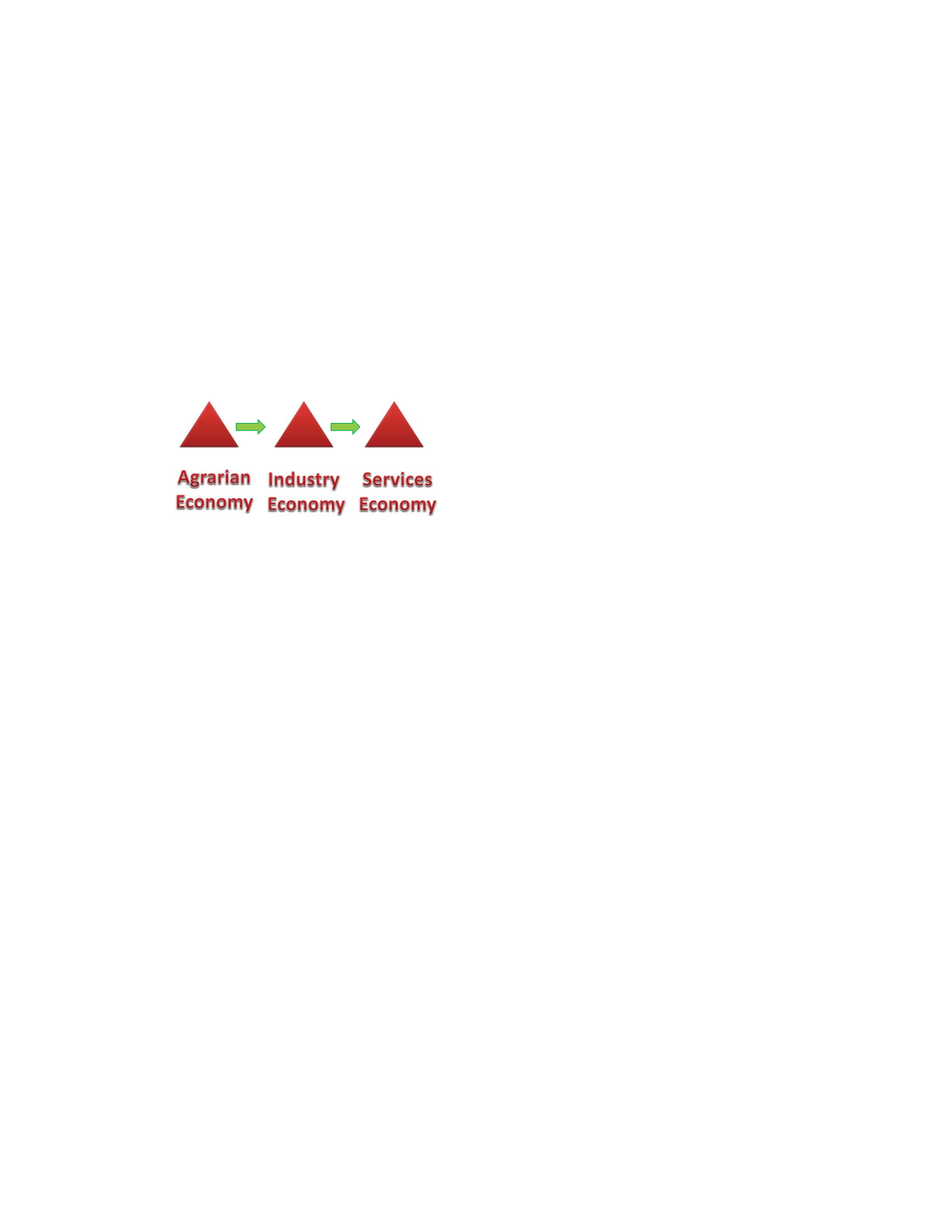
Figure 1. Traditional linear growth model.
The historical observations of economic development was linear, starting with an
agrarian-dominant economy, an industrial revolution would eventually change a farming
community to a manufacturing community and industrial labor force? Then, after a
while, the cost of living would increase and another change would take place, moving the
economy from a manufacturing or industry-dominated economy and labor force to a
service-dominated economy and labor force (see Figure 1).
20
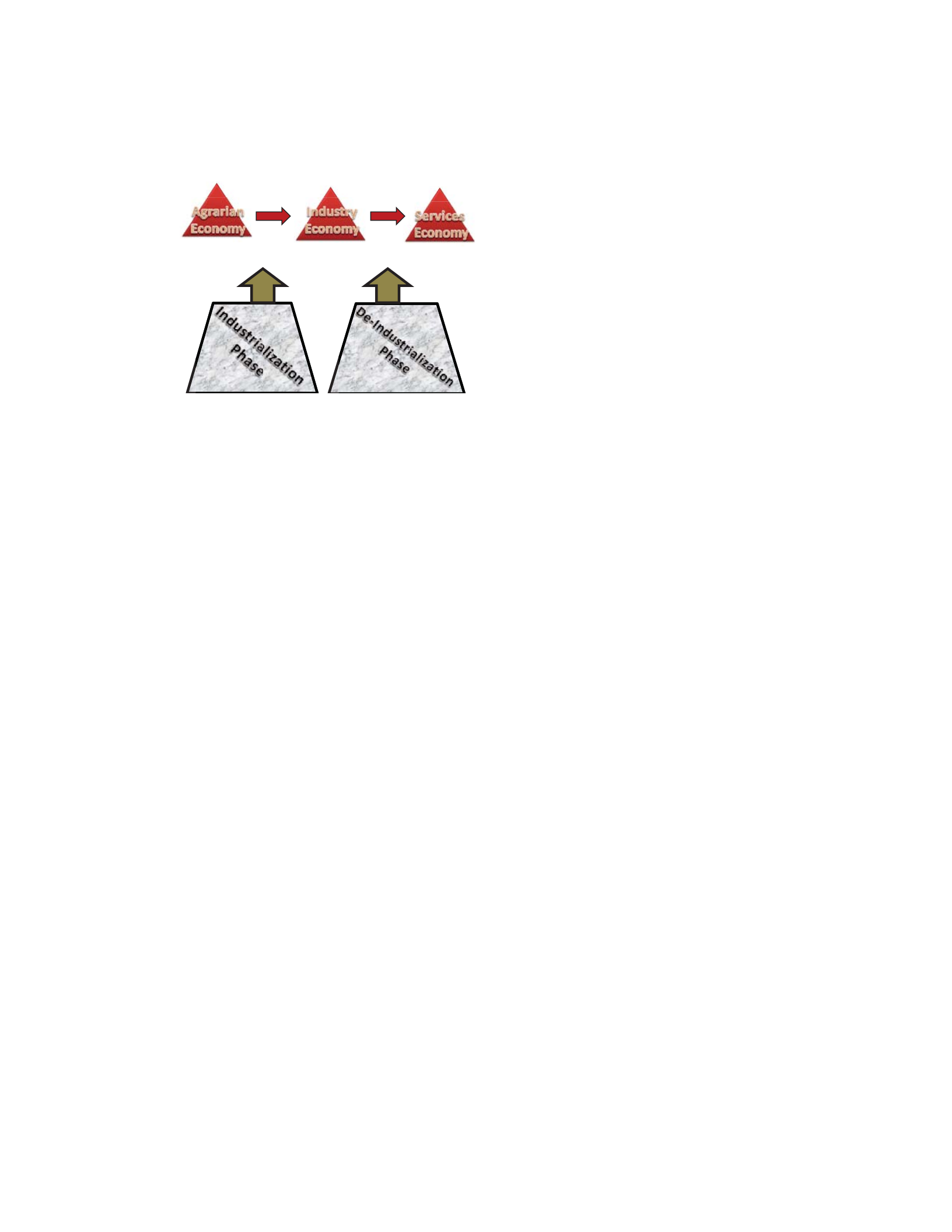
(First World)
(Second World)
(Third World)
Figure 2. Industrial Growth Phases.
In effect, the first nations to industrialize are sometimes referred to as the first
world. The first world has since deindustrialized and now the nations industrializing are
often referred to as the second world. The third-world is a label for the poorest nations,
those nations that have not industrialized and are agrarian-heavy. There is a great deal of
literature on both phases of industrial growth, known as industrialization (i.e., moving
from an agrarian to an industry economy) and deindustrialization (i.e., moving from an
industry to a services-dominated economy).
We now know that a linear growth model is an elementary tool of seeing the
world. It is, however, an easy way to explain grand observations. To economists,
however, this basic model simply leaves to many unanswered questions and need for
more developed models. As the understanding of economic development matures, so
must the models we use. The new BIED-GPM will build off of the three-stage linear
model observations.
Cleveland (2003) highlights the movement from an agrarian society to an industry
society and the change in research trends when stating, “Growth theorists are abandoning
a long-held hypothesis originally proposed by Kuznets. . . that growth necessarily

21
requires initially greater inequality, as surplus workers are drawn from an inefficient
agricultural sector into a modern industrial sector” (p. 2). Cleveland continues to
elaborate on land’s inclusion in economic development models as natural capita, which
is seen often in environmental economics (Cleveland, 2003, p. 2). Land is considered to
be a primary element in economic models.
China
GDP Model
China
Labor Force by Occupation Model
Agrarian Industry Services
vs.
Agrarian Industry Serv
ices
9.60% 46.80% 43.60%
38.10% 27.80% 34.10%
Figure 3. China Example
An example of how indicator values change a model can be seen between GDP
composition by sector and labor force by occupation (see Figure 3). The CIA World
Factbook (CIA, 2011, p. 139) breaks down statistical information using the linear model,
agrarian, industry, and services sectors. Using the indicator of GDP, China has 46.8% of
its GDP-composition by sector coming from the industry sector, while only 43.6% of its
GDP is coming from the services sector. Only 9.6% of China’s GDP comes from the
agriculture sector (CIA, 2011), since the largest percentage of China’s GDP is coming
from the industry sector, China may be seen as a second world nation. In contrast, when
a different indicator is used, for instance, including labor force by occupation, China has
38.1% of its labor in agriculture, 27.8% of its labor force in industry, while it has 34.1%
of its labor in the services sector (CIA, 2011). If we used the behavior of the labor force
to depict China’s measurement on the traditional linear example, The People’s Republic
of China would be seen as a third world economy. If we use GDP, China would be
labeled a second world nation. Which of these two indicators is a better measurement?

22
Looking at the two, one is a byproduct of behavior, that of GDP, which is an outcome.
Labor force by occupation is a description label of actual behavior, or an input. Behavior
input is a stronger indicator for group analysis. However, it might be helpful to use both
indicators in a supporting model, one that considers the behavior of the labor force by
occupation as well as the GDP composition by sector.
In an article titled “A Classical Model of Distribution, Productivity and Growth,”
Cleveland (2003) highlights Adam Smith’s use of the modern three-factor model and
contributes Smith with the notion of high concentration of land ownership and how it
negatively impacts productivity (p. 1). Cleveland (2003) discusses the importance of
balance and equilibrium, but also highlights the principles of three primary elements in
most economic models: land, labor, and financial capital in models as early as Smith.
Figure 4. Economy Triangle
It is possible to reclassify all of these categories into three main disciplines, to
better conceptualize the moving pieces (see Figure 4). Using Smith’s (1776) classical
theory, all economics may be boiled down to labor capital, financial capital, and natural
resource (land) capital. These three main elements are named different things over the
years, but nevertheless can be identified clearly as the fundamental building blocks of
23
economics. Therefore, three key academic subfields in economics should be better
understood: behavioral economics, financial economics, and environmental economics,
the study of each core model element. When put together in a triad, these primary pillars
of economics help conceptualize what can be called an economy triangle. The triangle
can grow or shrink, but can be represented in a visual format as done in Figure 4. The
academic discipline is represented in red (behavioral economics, financial economics, &
environmental economics) and the primary economic capital resources are represented in
green (labor capital, financial capital, & natural resource capital). Cleveland (2003)
endorses this type of model, stating “I believe that a three-factor model build on land,
labor and capital best captures the essence of the institutional view, including that of
Adam Smith, and yields the most productive insights on the relationship between
inequality, productivity and growth” (p. 2).
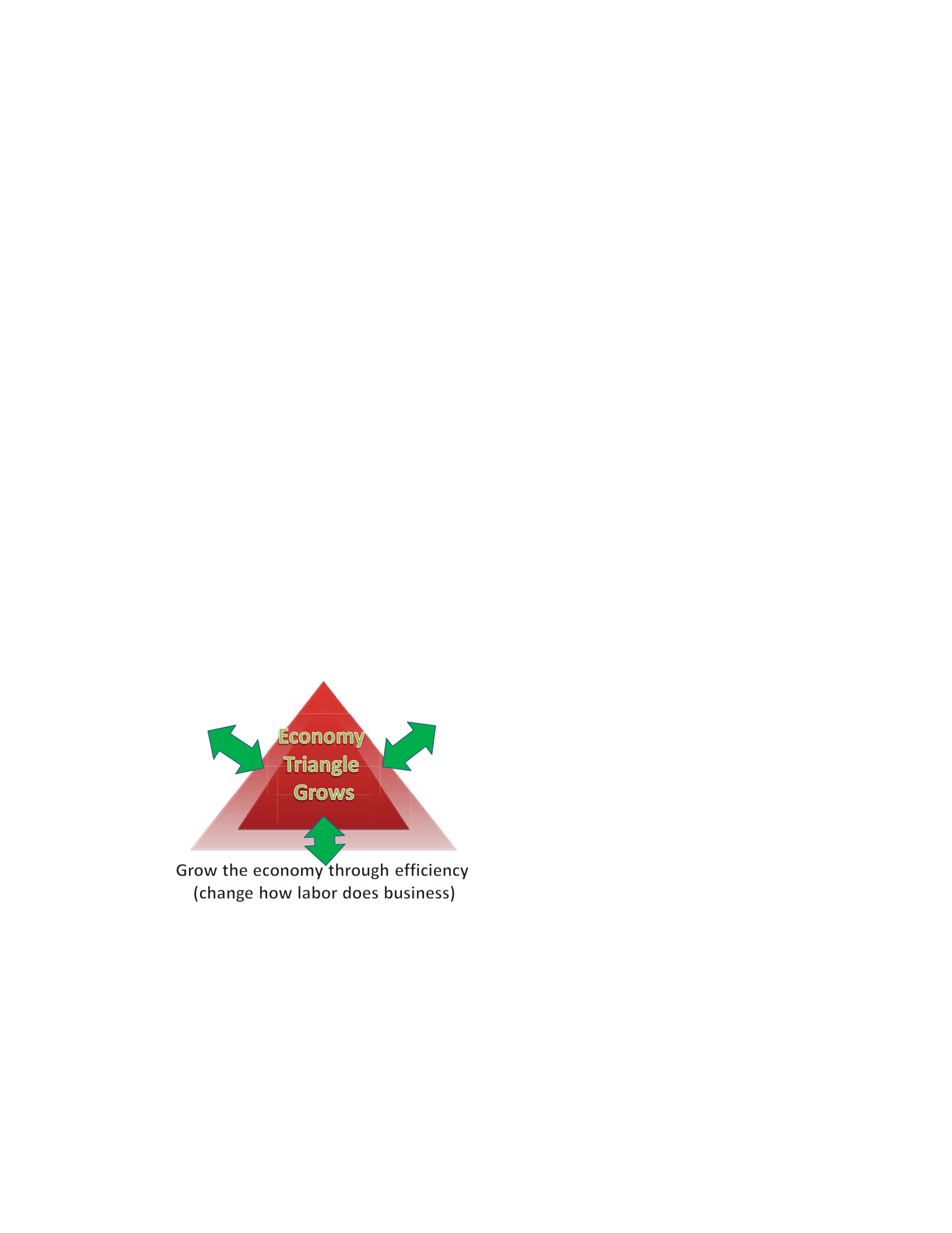
Figure 5. Economic Growth
Economic Growth Theory vs. Development Economic Theory
The study of economics is a dynamic discipline. Economic growth is the
subsector of economics that highlights attention towards growth or expanding the
economy (i.e., growing the triangle, see Figure 5). Development economics, however,

24
uses economic growth, but is really focused on moving an agrarian society to an industry
society or industry to services change (i.e., linear industry growth phase movement).
Recently this discipline has been focusing on what has been named sustainable growth,
which is another way of saying reasonable, steady, and predictable growth with
limited/no negative slides or cycles. Growth economics is focused on doing what one is
currently doing better, while development economics is focused on changing what one is
doing both economically and through labor trends (see Figure 6). The thought is that if a
nation is able to change what it is doing to move toward a more advanced type of
economy (i.e. agrarian to industry or industry to services), then it will by default increase
the economic growth potential of the economy. Both have the same end state as a goal, it
is the path and approach that is different.
Figure 6. Economic Development.
It is understandable why such attention is given to sustainable growth. A nation-
state that has steady positive growth can manage public administrative affairs easier than
a nation that changes from large growth patterns followed by negative growth years.
Even if the average of the positive and negative years turns out to be a reasonable growth

25
rate, the “management” of the society in the negative years becomes problematic.
Predictability becomes important when managing a society; therefore steady and
predictable economic growth is desirable to uneven or unpredictable growth.
Economic growth promotes the increase of one or more of the three primary
elements: labor capital, financial capital, and natural resource capital. Labor capital, or
those actually doing economically viable activities, is one of these primary elements.
When the labor force increases the potential for growth in that side of the economy
triangle increases. The labor force is where we will bring behavior into the model.
Natural resource capital is another key component in many models. This consists of the
raw materials found within the systems borders to include land. As science
advancements get better, the ability to get to some of these resources increases leading to
the growth of this side of the economy triangle. Financial capital is a versatile and
important component because it can be used to procure needed items that nations may
require but do not yet possess (e.g., labor or material) often called substituting. Financial
capital is sometimes measured in savings rates or, later, as “access to capital,” referring to
loans, foreign direct investment, aide, etc. Ultimately it is the access to money that grows
this side of the economy triangle. This is also where we start to see the cost of doing
business. If the cost of doing business is too high, financial capital won’t increase.
These are only quantitative measurements, however. When emphasis is given to the
education of the labor force or the quality of labor, a more dynamic understanding takes
place. When emphasis is not on how much oil a country has, but what type of oil and
where is it located. Is it easily accessible? Is it near a production facility or near a port?

26
Are financial capital resources new money or old money? Important research is devoted
to determining what type of capital (e.g., financial, labor, or natural resources) is more
valuable. The use of both quantitative and qualitative measurements can help capture a
stronger understanding of such a complex topic.
Together labor, financial, and natural resources make up a nation’s capital
markets. An economy is made up of numerous systems that are all actively participating
in the economy. Each system has organizational knowledge, political maturity, and
interacts with other systems differently over time. Marx (1867) contributed to the
premise of ownership benefits with what is called the “means of production” or the
ownership of a system output. The means of production becomes important when
studying different systems, as those who own the activity typically benefit the most.
Economic development is focused on growing the economy through changing the
business of labor. Unlike economic growth, which is focused on expanding the economy
through learning how to do the business better, those in economic development actually
attempt to change what business you are doing (e.g., agrarian to industry or industry to
service). Behavioral nuances are important. In reality both economic growth and
economic development strategies attempt to increase the size of the economy, but
through different means or paths.
Kooros and Badeaux (2007) contribute to the nuances between economic growth
and economic development stating, “Economic development, distinguished from
economic growth, results from an assessment of the economic development objectives
with the available resources, core competencies, and the infusion of greater productivity,

27
technology and innovation” (p. 120). They continue, “As well as improvement in human
capital, resources and access to large markets” (Kooros & Badeaux, 2007, p. 120). The
discussion identifies that nations that pursue economic development or economic growth
face the following concerns: “…foreign debt conversions into foreign direct investment,
foreign debt investment (FDI) privatization of economic activities; trade regionalization;
conversion of import-substitute investments into export-expansion investments;
technology transfer; co-production, and many other sound economic decisions” (Kooros
& Badeaux, 2007, p. 121).
The economic community is divided on how to classify theory. In the area of
development economics, the best way to classify theories or schools of thought is still not
agreed upon. Verspagen (1992) identified four classifications when he wrote
Endogenous Innovation in Neo-Classical Growth Models: A Survey. This work captures
the historical theoretical context primarily on technological change and economic growth.
At the time, Verspagen (1992) outlines four schools of economic growth: 1) the Neo
Keynesian School, 2) the post-Keynesian School, 3) the neo-classical school, and 4) the
new neo-classical school. In contrast, Ricardo Contreras (1999) writes in Transnational
Law and Contemporary Problems about four different schools: 1) structuralism, 2) the
linear stages growth model, 3) the neo Marxist-dependency theory, and 4) the neo-
classical revival. This is a strong example of the conflict in economics today. Five of
these eight categories counter another thought. One is solely based on a model, or a tool
used to identify whether a thought is strong or weak and should not be considered a
theory or a school of thought. My research categorizes the main themes in this discipline

28
by behavior and combines Verspagen and Contreras’s lists. I will attempt to identify
behavior as a driving factor in the classification of literature themes and avoid labeling
with words like “neo” or anti-schools.
Since this study explores existing models for strengths and weaknesses in order to
build a better model, let us start by examining the literature through a model lens.
Classical theory, as I see it, is about finding the simplest classification of basic building
blocks of an economy. Structuralism is focused on political decisions to substitute
missing capital (i.e., financial, labor, or natural resources) through import substitutions.
Using the economic triangle, if a nation does not possess the building blocks within its
political border, it needs to go out of the border to do business. Neo Keynesian and post-
Keynesian both refer to different ways of looking at economic problems from British
economist Keyes (1936). Verspagen (1992) refers to neo-classical models, mainly
Solow’s (1956) model, which was named the neo-classical growth model because “it
assumed that technological change is exogenous to the economic process” (as cited in
Verspagen, 1992, p. 631). This means that the model that spearheaded the neo-classical
movement was simply reaching beyond the system to explain the long run rate of growth.
Verspagen (1992) writes, “In the first neo-classical growth models, technological change
was reduced to an exogenous phenomenon, basically for analytical convenience” (p.
366). The limitations of a model should not limit the theory, though in development
economics, it often does. Finally, the evolution of theory after exogenous theory is
endogenous growth theory, which means to look within the economic system to explain
what is happening. The biggest flaw in the collection of classifications listed lies in

29
whether or not a nation-state grows endogenously and exogenously simultaneously. Of
course, growth from external and internal events can happen together, but the academic
discipline is not there yet. Some like to think that exogenous and endogenous theory
refers to implications within the model or outside the model factors. If this is true, then
why not build a bigger model? Therefore, instead of referring to the classifications as
schools of thought, let us consider that the following three categories are more era-
specific and tend to depict what the majority of research was focused on during that time
frame.
There are three eras of economic growth that will be considered. They are the
World War Era (1930s, 1940s, and 1950s), the Post-war Era (1960s, 1970s, and 1980s),
and finally, the International Organization Era (which includes the 1990s, 2000s, and
2010s). There are several theories that are explored during these eras including classical
growth theory, productivity growth theory (also known as neo-classical growth theory),
exogenous growth theory, endogenous growth theory, international organization
taxonomy growth theory, and behavioral growth theory. The models that are used in
each era add to the body of literature and the overall understanding of economic growth
and, ultimately, economic development.
Here is an example of the new way of looking at information. The dominant
model in the neo-classical growth school of thought is known as the neo-classical growth
model. The real behavior in the neo-classical growth school is productivity. The most
useful outcome of this school is total factor productivity. It is, however, referred to as

30
neo-classical growth often but will be referred to as productivity growth henceforth,
when labeled on behavior and not after the model name.
I have chosen three eras in which to highlight the dominant thoughts and models
of that time (the World War Era, the Post War Era, & the International Organization Era).
This has been done to simplify the complex body of work in both development and
economic growth research. Since I am interested in economic growth as it relates to
development economics, I will tie the two together, and look at examples of models in
both areas, in an attempt to bring the two disciplines closer together in a mutually
supportive and beneficial way.
Economic Behavior Theory
Behavior economics is usually focused on demand or consumer selection choices.
When looking at the choice to enter into a job that is in the agrarian sector or industry
sector, behavior economics is also present. The life cycle of spending requires the means
to make funds first to then spend. I look at behavior economics to be important to
occupation sector selection.
Camerer and Loewenstein (2002) state that “…the core of behavioral economics
is the conviction that increasing the realism of the psychological underpinnings of
economic analysis will improve economics on its own terms—generating theoretical
insights, making better predictions of field phenomenon, and suggesting better policy” (p.
1). Camerer and Loewenstein write in their article titled, “Behavioral Economics: Past,
Present, Future” when they contribute, “behavioral models will gradually replace
simplified models based on stricter rationality, as the behavioral models prove to be tract

31
able and useful in explaining anomalies and making surprising predictions” (p. 48).
Camerer and Loewenstein identify the origins of behavioral economics stating, “When
economics first became identified as a distinct field of study, psychology did not exist as
a discipline” (p. 3). As each discipline matures, it becomes clear that both development
economics and behavioral economics can benefit from the other.
Solow contributes to the behavior discussion noting, “The permanent substructure
of applicable economics cannot be too very large because social institutions and social
norms evolve, and the characteristics of economic behavior will surely evolve with them”
(Solow, 1987, par. 55). Solow identifies economic behavior will change and this study
helps study that change in greater detail.
Quantitative and Qualitative Methods
The three main pillars of the economy triangle are labor capital, financial capital,
and natural resource capital. All of these can be measured using a quantitative or a
qualitative method. Labor capital could be described as a population of a nation. To be
more specific, it could be refined to actual working age labor, but this operationalization
is quantitative in nature. What do these categories really mean on their own? Qualitative
measures may be used to help identify degrees and more specifics, like the average
education level of the working age labor. This concept implies that some labor is better
than other types of labor or that the quality of an indicator matters in addition to quantity.
Kuznets won the Nobel Prize in 1971 for his work on modern economic growth.
Kuznets (1971) added to the method dialogue that “the quantitative base and interest in
economic growth have widened greatly in the last three to four decades, and the

32
accumulated results of past study of economic history and of past economic analysis”
(par. 29). Kuznets continues, “Economic analysis could be combined with the richer
stock of quantitative data to advance the empirical study of the process” (Kuznets, 1971).
Kuznets (1971) identifies the separation in quantifiable economic models from that of
qualitative grounding. While the trend moved to quantifiable data 40 years ago, it now
needs to move back to qualitative foundations. This is starting to happen with work on
human development indicators and the beneficial work of the United Nations (UNDP,
2012).
Economic System Classifications
Systems have observable behavior. Understanding the main elements of systems
can contribute to the understanding of the interaction between labor capital, financial
capital, and natural resource capital, the economic triangle (the foundation to all
economic models or schemes). These systems are typically recognized by the political
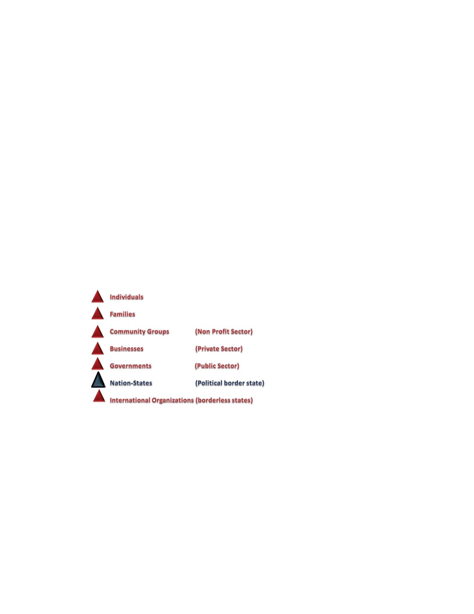
structure as main players in the game of economics (see Figure 7). From smallest to
largest, the main systems can be labeled as follows: (a) individuals, (b) families, (c)
community groups, (d) businesses, (e) governments, (f) nation-states, and (g)
international organizations. These different systems work together and against one
another. All systems include the smallest system: individuals. Most individuals belong
to families, so the family system contributes and is impacted by the other systems. The
concept of a business as an independent system is a key element to modern development.
There are countless systems. Only the primary systems are identified here, because it
will become important to distinguish between them later. When dealing with
33
international studies, nation-states are typically the main players. Finally, international
organizations are really a phenomenon that grew after World War II. International
organizations have significant impact and influence in modern models.
International organizations dominate some of the newest models, with growing
collections of data and international clout & visibility. With the invention of the internet,
many researchers look to international organizations to check or cross check individual
nation state data bases. Many nations do not have the capacity to collect international
information and rely on international organizations for key comparison and decision
making data.
Figure 7. Economic Systems Classifications.
Using economic systems is a way of classifying different behavior. Governments
act differently from businesses. It is important to study systems, because the better we
get at classifying groups and recognizing their behavior, the more accuracy we will have
in the analysis. This study is an international comparison study, so most of the attention
is on nation-state systems. I focused on the economic path each nation has taken and
identify the options that are available as well.

34
Measurement and Assumption Problems
Let us for a moment attempt to think about a common economic problem: How
can economic development happen? If economic development is made up of three
primary elements, and any of these increases with no negative growth in the other two
elements, then positive gains are made to the economy (i.e., the economy triangle gets
larger). This is called economic expansion. We know, however, that all three elements
are usually moving; in fact, we have a difficult time really measuring any of these three
elements. Solow (1987) writes about assumption, stating “I would like to remind my
colleagues and their readers that every piece of empirical economics rests on a
substructure of background assumptions that are probably not quite true” (par. 41).
The population of a nation-state is always fluctuating. It is difficult trying to
identify who is actually working, who is working two or more jobs, and so on. Who is
working full-time, part-time, and who is working under the table, promoting a black
market economy? There are difficulties identifying undocumented immigrants and
emigrants. Money is made through legal and illegal methods. It becomes difficult to
identify how often money moves between these numerous systems (although countless
labor hours are devoted to just that). Then, when one attempts to calculate money
exchanged through barter, foreign exchanges, lost money, and/or counterfeit currency—
especially in an electronic currency environment—limitless calculations exist. Finally,
any attempt to calculate actual natural resources becomes equally tricky as both legal and
illegal methods are used. Until all of the oil or copper is extracted from the ground, one
can only estimate how much one has. Then there are legitimate reasons to not want the

35
actual number of resources within a system publicly known. Ultimately, there is a
measurement problem in economics. Therefore, a degree of acceptance is required to
better understand and appreciate these measurement shortcomings. Measurements at the
international level are dependent upon many things.
While data collection is getting better, it is still susceptible to significant error.
This is important to note, not because analysis cannot be made, but to identify the
shortfalls in collection at such a macro level. Kuznets (1971), in his Nobel reception
speech, says, “It seems fairly clear that a number of analytical and measurement
problems remain in the theory and in the evaluation of economic growth in the developed
countries themselves” (par.32). Kuznets continues, “One may look forward to major
changes in some aspects of the analysis, in the national economic accounting, and in the
stock of empirical findings, which will occupy economists in the developed countries in
the years ahead” (Kuznets, 1971). Indeed we have seen just that.
Figure 8. Triangle Economy Model.
This literature review is about economic models. It is, therefore, important to
recognize that all models have assumptions. It is these assumptions that often get
overlooked. Let us consider an equation of three unknown variables (see Figure 8). How

36
can we identify the value of one variable? If one has an assumed value of two of the
variables, we can come up with a value for the third, but that is only true if one agrees
with the assumptions of the first two values. Models are tools and they can help provide
significant insight into complex economic problems. Like tools, however, if used
improperly, misleading insight is possible. Development economics has used models to
help clarify dominant social concerns. Take, for example, the Great Depression in the
1930s. The unemployment issue was at the top of government priority lists around the
world. Therefore, it should be expected that the models that were developed in that
decade were directed mainly on labor issues. It is also critical to identify some important
behavioral economic assumptions. Group systems act differently and it becomes almost
impossible to clearly differentiate behavior between the countless systems). This is
because an individual can be part of a family, extended family, businesses, a religious
group, nation-state, regional organizations, and possibly even international organizations.
Any individual can belong to many different systems at one time. Priorities may change
over time for the individual and for each system as well. Productivity theory (neo-
classical thought) has shed significant insight into this dilemma, but there is still a long
way to go. The lens through which a problem is viewed is important. Many existing
models fall into a different theory classification. Some may fall into more than one
theory as well. This becomes important as we attempt to boil down different systems to
get a clearer view of what may be happening. The assumptions we make to get one value
may not be accurate. If they are not, then the results will invariably be affected. The
type of model, the lens, and the assumptions made will impact the final analysis. As we

37
review some of the key models, perhaps we can view some old development problems
through a newer behavioral lens.
Kuznets (1971) contributes to this discussion in the following:
The lag has been in the analysis of these data by economists and other social
science scholars, because of the scarcity of such scholars who cannot be spared
for research within the less developed countries themselves and because of the
natural preoccupation of economists in the developed countries with problems of
their own countries. One may hope but with limited expectations, that the task of
refining analysis and measurement in the developed countries will not be pursued
to the exclusion or neglect of badly needed studies of the less developed
countries, studies that would deal with the quantitative bases and institutional
conditions of their performance in addition to those concentrating on what appear
to be their major bottlenecks and the seemingly optimal policy prescriptions. (par.
32)
The resources needed to conduct economic activity can be found in the
economy triangle which uses three sides represented as capital assets. These
capital assets are labor, financial, and natural resources. Learning how to grow
the economy or economy triangle requires the identification of each side. Once
the “sector” is identified, measurement of it is needed. This requires both the
quantity and quality of each indicator be defined.
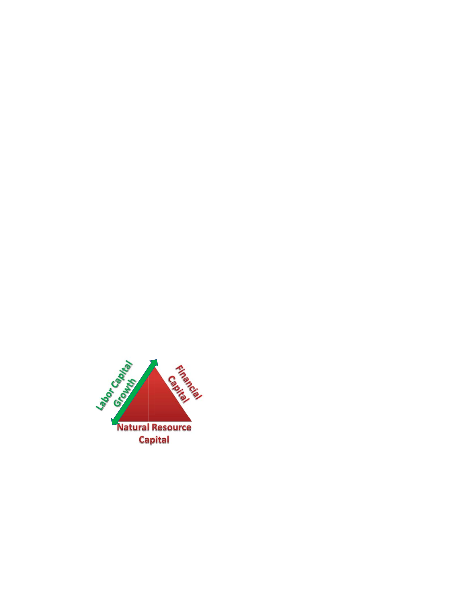
Labor Capital Growth
38
Labor capital is the first pillar to the economic triangle (see Figure 9). Labor
capital growth can be broken into two categories: One is demographic or quantitative in
nature, such as birth rates, life expectancy, and immigration; the other is qualitative in
nature, such as education level, literacy, and experience level. Labor can and does move
between systems. Growing the labor capital means both getting more workers, and
getting better workers. Unemployment becomes important to this resource, as balancing
how many workers with available jobs is important to any economy. Steady and
predictable growth is the goal. One thought is that in order to move from an agrarian
society to a manufacturing society, you have to have excess labor first. Furthermore,
some believe that advances in farming technology simply freed up labor to move to the
city to pursue industry. Which came first is still a topic of discussion, but identifying that
labor is a key element in economic models is critical as it is one of the three basic
building blocks in all the models we review.
Figure 9. Labor Capital Growth
Aghion and Howitt (1997) discuss this important economic building block in their
work titled endogenous growth theory. Garcia-Penalosa (1998) contributed in this work
39
with a section titled “Problems and Solutions,” by writing, “Although the absolute size of
population is irrelevant, its rate of increase is not.”(p. 14) Garcia-Penalosa continues:
Because faster population growth will tend to reduce the amount of capital per
person in much the same way as faster depreciation would, not by destroying
capital but by “diluting it”—by increasing the number of people that must share it
(Garcia-Penalosa, 1998, p. 14).
In recognizing the importance of labor capital in the broader economic spectrum,
2010 was a significant year. Pissarides, Mortensen, and Diamond gave three Nobel Prize
lectures on labor capital titled, “Equilibrium in the Labour Markets with Search
Frictions” (Pisssarides, 2010), “Markets with Search Friction and the DMP Model”
(Mortensen, 2010), and “Unemployment, Vacancies, Wages” (Diamond, 2010),
respectively. These three speeches reinvigorated interest in the labor discussion.
Financial Capital Growth
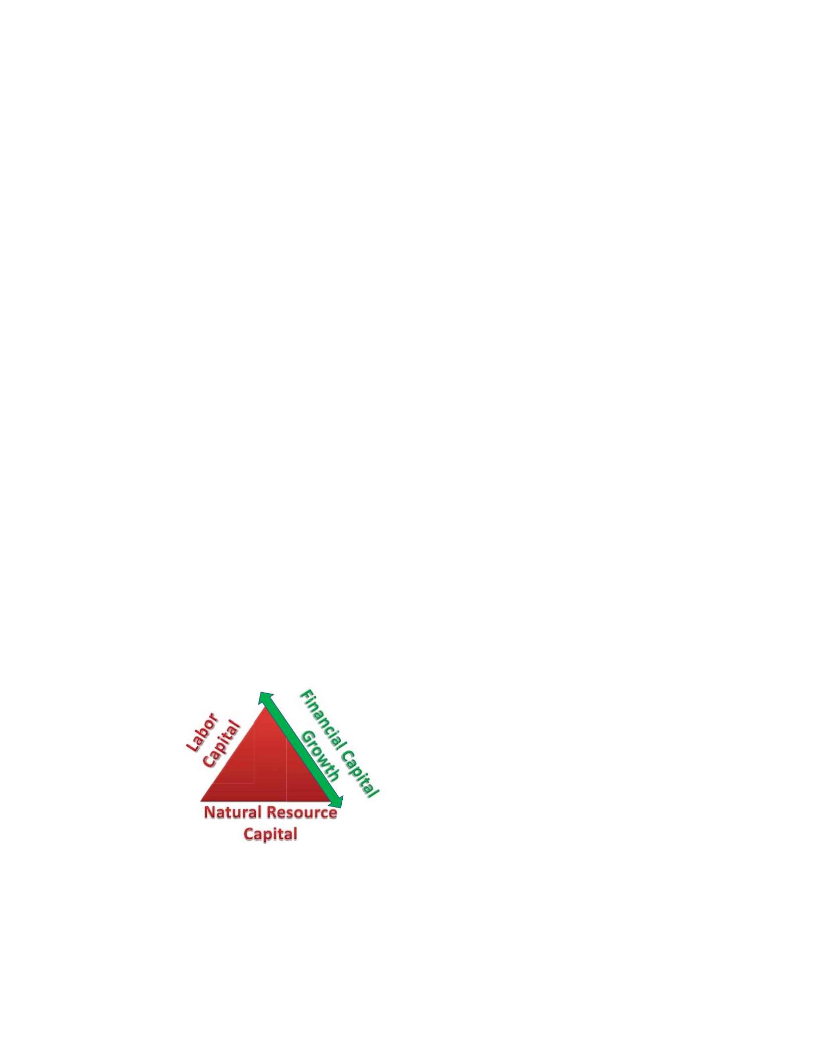
Financial capital growth is the second pillar to the economic triangle (see Figure
10). It is another key component in almost all economic models.
Figure 10. Financial Capital Growth.

40
It is broken into qualitative and quantitative categories as well. When society
moved from a barter-dominated economy to a currency economy, several advances
occurred. The saving of money would allow a buildup which could be used for
development investment. Marx (1867) highlighted the means of production as integral to
economics, as mentioned earlier. Who owns or benefits the most from economic activity
is important. Ultimately, Marx (1867) was concerned with qualitative issues. If an
economy is missing resources, financial capital can be used to obtain extra labor or
additional natural resources in order to pursue efficient production cycles and balanced
growth. Other factors come into play in this sector. Having money is important, but
having access to money is critical as well. Loans and the ability to borrow have been
found to be positive as well. Attracting foreign direct investment or aide is also seen as
beneficial to the receiving system. Some models will focus on what type of money is
more important given the circumstances. The knowledge that money is a key component
to economic modeling and that different types of money have different values will help as
we review historic development models and modern models.
Natural Resources Capital Growth
Natural resource capital is the third primary element in the economic triangle (see
Figure 11).

41
Figure 11. Natural Resources Capital Growth.
Just like the first two pillars in the economic triangle, it is also found in most
economic models. It refers to resources such as minerals, crops, water, oil, and trees.
Mining, drilling, fishing, and farming are all behaviors that develop and use natural
resources. It should be easy to see that the person who owns these resources will benefit
the most. When kings owned all the land, it was the king that benefitted the most from its
development. When property rights and rule of law came into favor, the average person
obtained access to benefit from land development. This is a key element to most
economic models. Quantity and quality will become important when studying this
resource. Different resources have different values. When looking through a lens of
efficiency under the king example, those working the land did so with minimum personal
benefit. Thus, if land ownership changes, than the benefit to those actually working the
land will increase, this makes the overall system more efficient and all economic
decisions should be about efficiency.
Historical Background

42
Before we look at the dominant economic growth models in the last 90 years, we
need to appreciate the historical background that brings the discipline to the point at
which economic models contribute as they currently do. Classical growth theory and
belletristic growth models can be attributed to the late 1700s and the work of Smith.
Smith is often thought of as the founding father of modern economics. Smith’s main
work, An Inquiry into the Nature and Causes of the Wealth of Nations, was published in
1776. It is important to note the global climate during 1776, as the United States gained
independence this year on new economic principles. The British colonialism was
beginning to wane and a new economic and political chapter was emerging. Smith is
known for his “invisible hand” analogy and the concept of the free market. He focused
on three primary indicators: capital, labor force, and land. Two main themes of his work
are the contributions of economies of scale and the division of labor (Smith, 1776).
Classical growth theory was pursued in the 1800s by Ricardo and Malthus.
Ricardo added technology to his modeling in addition to Smith’s previous model
indicators. Ricardo is best known for coining the term, comparative advantage. His
work published in 1817 titled, The Principles of Political Economy and Taxation, focuses
on getting a product or service to market first to leverage the return (Ricardo, 1817).
Significant attention is given to technology as a driving force in economic growth. It
should be noted that Ricardo wrote his main work shortly after the War of 1812. This is
of particular importance, in that the international community was watching the United
States and Britain to see how future international economic relations were going to be

43
impacted. With the United States’ victory, colonialism as it was known faded, and a new
chapter in economic behavior was secured.
What is so important about comparative advantage is the addition of time and
market into the discussion. Not only does it matter what is being sold, but also when and
where. Both the quantity and quality of sale items is important. The notion of time and
market are pivotal concepts in development economics. The market can be seen as the
location, or the distance it takes to get to the buyer. The size of the market is also
important, as some markets are bigger than others and the quality of buyers is pertinent as
well. The quality of modern markets is an area of research that could benefit the
economic growth and development models when advances are made in measuring
markets.
Malthus published six editions of An Essay on the Principles of Population in the
early 1800s. He focused on indicators such as national income, profit, wages, and
capitalist consumption. Malthus (1798) is known primarily for his work with the labor
force, however. Together, Smith, Ricardo, and Malthus pioneered the new discipline
known today as classical theory of growth. Significant global events during this era
include colonization (the focus on natural resource procurement), slavery (the distortion
of the labor force), and mercantilism (a new means of production and trade).
One of the great examples in economics is the United States during the Civil War.
The North, dominated with factories, and the South, dominated with farms, ultimately
disagreed on the issue of slavery. This can be seen, however, as a development issue
over labor. The distinction between the types of economies in the North and South

44
promoted different types of behaviors. This is outlined in what later becomes the global
North-South debate. In reality, it is a farming and industrialization debate. The insight,
however, comes from observing the different behaviors in the farming economy and the
industrial economy. Ultimately, we know that the North won the war. If one takes the
position that industrialization is the driving force for human rights (maybe because the
focus on business systems promotes less need to dominate labor for financial benefit),
then economic progress is good for equality. The means of production comes into play,
however.
Arrow (1972) addresses a war’s impact on supply and demand in the following
statement:
The history of the capitalist system has been marked by recurring periods
in which the supply of available labor and productive equipment available
for production of goods has been in excess of their utilization, sometime,
as in the 1930s, by very considerable magnitudes. Further, the relative
balance of overall supply and demand in the postwar period in the United
States and Europe is in good measure the result of deliberate governmental
policies, not an automatic tendency of the market to balance. (par. 3)
In the farming example, the plantation owner owned the labor. In the
manufacturing example, the business does not own the labor, but creates the opportunity
for individual gain by choosing to work at the factory. The incentive for the worker in
the North to work hard was positive, while the incentive for the slave to work hard in the
South was not. Ultimately, the factory system is more efficient because both the business

45
owner has incentive to work hard and the laborer has financial gain from working hard.
It is not hard to see why one was more successful than the other. Creating a more
efficient system should be the goal of all economics.
This example brings up another concern, one of group behavior. If the agrarian
sector is tied to weather and seasons (which are not reliable), and industry is not
constrained by these elements, it can be stated that industry is more reliable than the
agrarian sector. Generally, industry is more consistent, which is better for planning
purposes. Just like the budget example for a nation-state, steadiness and consistency is
preferred.
Era 1: World War Era (1930s, 1940s, and 1950s)
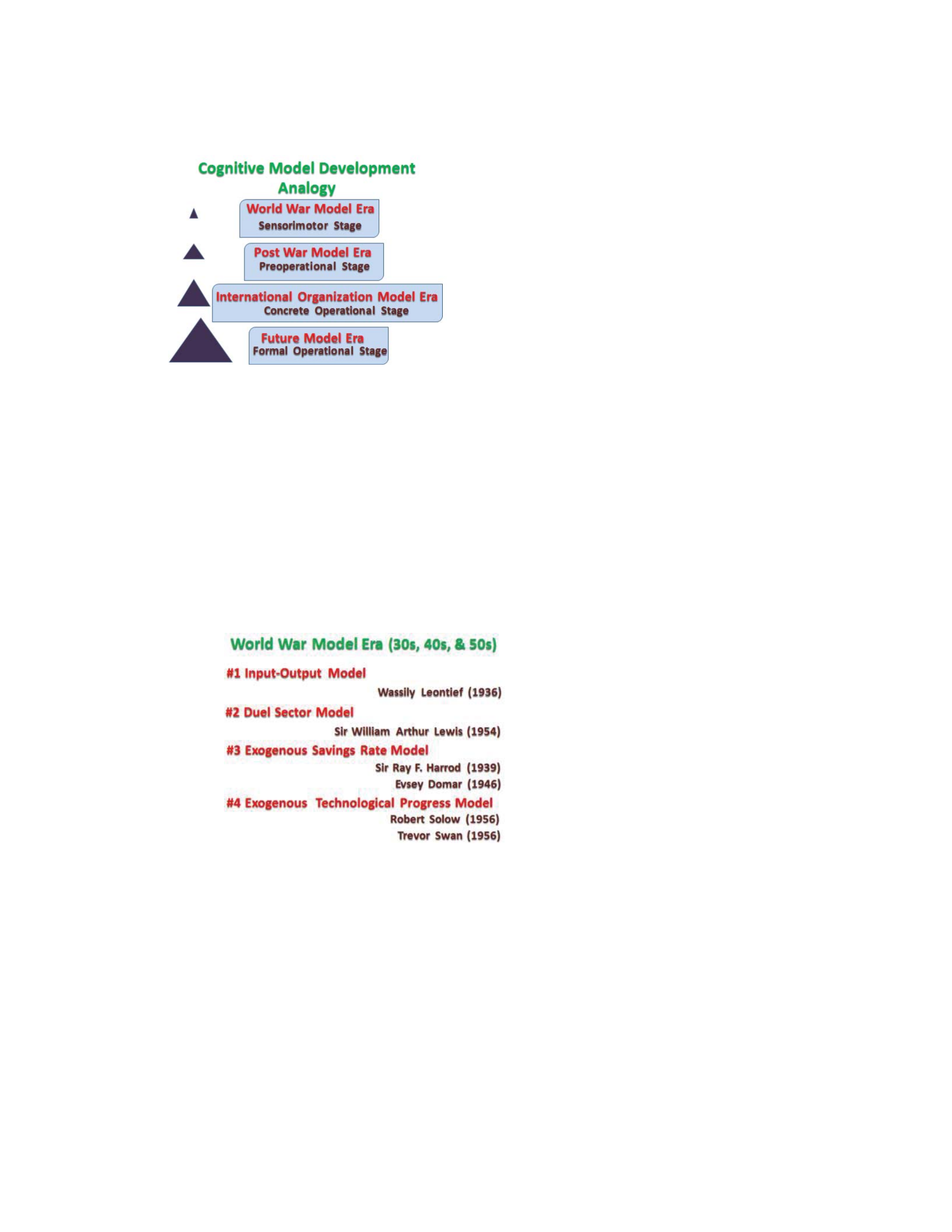
The schemas (Piaget, 1964), or way of organizing information, were set during
the historical period we just reviewed. Using Piaget’s (1964) theory of cognitive
development, we learn that of four distinct stages of development, the use of economic
models, at best, might best fall into the third stage, or concrete operations. The four
stages are (a) sensorimotor stage, (b) preoperational stage, (c) concrete operational stage,
and (d) formal operational stage (see Figure 12). One could argue that the World War
Era would embody the sensorimotor stage for economic models: Indeed, there is sensory-
motor causality in the four models we will review in this era. Piaget (1964) identifies
that the learning process in this stage sets the agenda for follow on stages, with “a series
of structures which are indispensable for the structures of later representational thought”
(p.19).
46
Figure 12. Cognitive Model Development Example.
The four models in this era that capture the most dominant influence on the
discipline of economic growth are: 1) the input-output model, 2) dual sector model, 3) the
exogenous savings rate model, and 4) the exogenous technological progress model (see
Figure 13). These four models represent the dominant models from the 1930s through
the 1950s.
Figure 13. World War Model Era.
Model 1: Input-Output Model
The input-output model was the work of Leontief (1947). The work titled
Quantitative Input and Output Relations in the Economics System of the United States
identifies the use of a matrix model that captures the life cycles of different industries in
the United States. The timing of this model was right in the middle of the Great

47
Depression, which was likely the motivation for the study. This study focused on one
country and broke down different industries in a methodical fashion.
Kooros and Badeaux (2007) write about the input-output model, praising “the
ingenuity of Leontief to provide an eloquent predictive system pertaining to the real-
world behavior through the formulation of this mathematical model” (p. 123). They add,
“Whereas to many it [the input/output model] was initially considered pure abstraction, it
is now a well-recognized model” (Kooros & Badeaux, 2007, p. 123).
Leontief eventually won the Nobel Prize in economics for his model contributions
and to furthering economic understanding through his matrixes. In 1973, during his Prize
Lecture, Leontief defines his model in his own words:
The world economy, like the economy of a single country, can be
visualized as a system of interdependent processes. Each process, from
the manufacture of steel to the education of youth or the running of a
household, generates certain outputs and absorbs a specific combination of
inputs. Direct interdependence between two processes arises whenever
the output of one becomes an input of the other: Coal, the output of the
coal mining industry, is an input of the electric power generating sector.
The chemical industry uses coal not only directly as a raw material but
also indirectly in the form of electrical power. A network of such links
constitutes a system of elements which depend upon each other directly,
indirectly or both. (Leontif, Structure of the world economy, 1973, p. 1)

48
Kooros and Badeaux (2007) write about Leontief and state the following about
the models that they reviewed: “Many countries aspire to formulate economic
development strategies to improve their quality of life” (p. 121). They continue stating,
“Development economics has lacked viable planning models” (Kooros & Badeaux, 2007,
p. 121). Leontief explains the model when accepting the Nobel Prize:
The state of a particular economic system can be conveniently described
in the form of a two-way input-output table showing the flows of goods
and services among its different sectors, and to and from processes or
entities (“value added” and “final demand”) viewed as falling outside the
conventional borders of and input-output system. As the scope of the
inquiry expands, new rows and columns are added to the table and some
of the external inflows and outflows become internalized. (Leontief, 1973,
p.2)
Leontief (1973) uses an example in his Nobel Prize Lecture of a world economy
broken down into two classifications, one of developed and one of less developed
nations. An example that is only divided into two groups may be seen as limiting in
scope and depth. His production matrixes, however significantly added to the
development economics discussion.
Model 2: Dual Sector Model
The dual sector model is a work of Lewis (1954). At the end of the Korean War,
Lewis wrote Economic Development with Unlimited Supplies of Labor. He later won a
Nobel Economic Prize for the efforts in defining the transition between an agrarian

49
economy and an industry economy (see Figure 2 and the Industrialization Phase). This
model is helpful in that it looks beyond political borders to capture a trend of labor
movement towards viable economic employment. When economic incentives are
advantageous, people will come. This refers to women and other members of society that
may not have engaged in economic activity until the incentives improve.
The concept of keeping labor constant in models is a common assumption, but
can be viewed as a model limitation. The concept of perfect competition is also very
common in models, but in the real world assumptions like these are unrealistic. In the
model world, however, it is a necessity to make assumptions in order to solve other
unknown variables to complete equations. Solow (1987) contributes to this discussion
during the Economic Nobel Prize reception lecture, stating “[Productivity] Growth theory
was invented to provide a systematic way to talk about and to compare equilibrium paths
for the economy” (par. 25) As a key author on productivity growth theory he states with
authority, “I am also inclined to believe that the segmentation of the labor market by
occupation, industry and region, with varying amounts of unemployment from one
segment to another, will also react back on the equilibrium path” (Solow, 1987, par. 26).
This thought becomes important when looking at the BIED-GPM in Chapter 3.
Kooros and Badeaux (2007) elaborate on this discussion when they reflect on a
dual system society:
Economic development transforms a traditional dual-system society into a
productive framework in which everyone contributes and from which
receive benefits accordingly. Economic development occurs when all

50
segments of the society benefit from the fruits of economic growth
through economic efficiency and equity. Economic efficiency will be
present with minimum negative externalities to society, including agency,
transaction, secondary, and opportunity costs. At the same time,
disintegration of national sovereign states into more fragmented nations
along the ethnic lines would not help these newly formed societies to
accede to a formidable economic development regardless of their form of
government. (p.120)
Model 3: Exogenous Savings Rate Model
Productivity growth theory probably encompasses the most models and includes
the third and fourth models in the World War Era category. The exogenous savings rate
model is from Sir Harrod (1939) and Domar (1946). Together, their research has become
known as the Harrod-Domar model, or when labeled based on behavior, it is known as
the exogenous savings rate model. This model focuses on exogenous growth and
primarily the individual and group behavior of saving. This activity can also be seen as
spending less than what is made. In practical terms, the benefit comes from positive
internal production cycles.
The main idea of productivity growth theory is the distinction between two
categories of systems: individuals, and groups or businesses. This separation identifies
individuals (and families) that will attempt to maximize utility, while businesses will
attempt to maximize profits. What is insightful about the theory is that it actually
identifies different systems and defines noticeable behaviors between them. Solow

51
(1987) had the following to say during his Sveriges Riksbank Economic Prize acceptance
speech on the exogenous savings rate model:
Harrod and Domar seemed to be answering a straightforward question:
when is an economy capable of steady growth at a constant rate? They
arrived by noticeably different routes, at a classically simple answer: the
national savings rate (the fraction of income saved) has to be equal to the
product of the capital-output ratio and the rate of growth of the (effective)
labor force. Then and only then could the economy keep its stock of plant
and equipment in balance with its supply of labor, so that steady growth
could go on without the appearance of labor shortage on one side of labor
surplus and growing unemployment on the other side. They were right
about that general conclusion. (par.3)
Model 4: Exogenous Technological Progress Model.
The fourth model in the World War Era is made up of two different authors, as is
the third model. Swan’s work on the rate of technical progress was combined with
Solow’s work and is now known as the Solow-Swan neoclassical growth theory, or the
exogenous technological progress model. Solow and Swan added to the Harrod and
Domar Models. With the growth of legal business entities and land rights, the economic
dynamics changed. Specific attention was drawn to the new industry sector and how its
behavior differed from agrarian practices. Shift work was a much different behavior than
farming or taking care of animals. It was less dependent on the weather and season
cycles as discussed earlier. The economic systems that operated in industry became

52
quickly dependent on skilled and reliable labor. The industrial sector became very
efficient using three shifts and keeping plants operational around the clock. This
efficiency made it profitable and increasingly more attractive to agrarian activities. The
labor force typically voted in opposition and moved to industry, which is tied to factories.
This phenomenon is seen in the moving from a rural area (i.e., where agrarian economies
exist) to city centers (i.e., where industry economies exist). It should be noted that
another difference between agrarian and industry sectors is where “the market” is located.
The two sectors are not equal regarding where people live and buy their goods. When
people live on farms and sell goods in the city, there are logistical costs involved. When
people live in the city and buy/sell goods in the same city, additional efficiencies are
realized. The agrarian sector is less efficient than the industry sector in this matter.
Another label for this transition is the “industrial revolution” or the Industrialization
Phase (see Figure 2).
Figure 14. External Production Cycle.
Exogenous growth theory is a collection of research that focuses on external
production cycle behavior. This is economic activity between other systems. In the
international realm, this is primarily nation-state activity with other nation-states.

53
Obviously, business level (private sector) activity happens, but it is collected at the
national level to compare against other national levels. The external production cycle is
made up from the cost of the cycle, plus the return of the cycle and equals either a
positive or negative growth. The goal of external production cycles or exogenous growth
models is to find the comparative advantage between systems using different political
structures and rules for economic gain.
The two driving forces behind dependency theory are Singer (1949) and Prebisch
(1945). The crux of their work is that trade after World War II was changing the known
rules of the international environment and the global competitive market. The countries
with money needed resources to grow and typically found cheaper resources in those
nations with little money. This seemed to put less developed nations at a disadvantage,
as the only good or service wanted by those with money would impact the terms of
procurement. This seemed to make the less developed nation “dependent” on the primary
income source (typically the industrialized world).
After World War II, the world was very internationally aware. Only the United
States had a modern economy without significant infrastructure damage due to the war.
This influenced how nations approached rebuilding modern economies, who lent, who
borrowed, and what the terms were. Also, the world was being divided by two
contradicting political thoughts: communism and capitalism. Though we now know how
this debate eventually ends, this was not clear in the 50s and 60s. Therefore, the
dominant observations were about development aid, monopolies, and natural resource
procurement. If labor moves to jobs, natural resources move to where labor is, and

54
money moves to where natural resources are, then the economic triangle would
demonstrate significant movement. This model places an emphasis on natural resources
and its movement toward industry production sites. Marx would be interested in this,
because it depicts a concern for who owns the means of production: The mining location
or market is a production site, but not the important end or more profitable production
site. Therefore, it is less beneficial than the industry market. The concept of a market is
the key here. Where is money actually being made? Indeed, profits can be made in
natural resources, but better profits typically exist in the industry phase. Thus, again a
distinction is made between the type of production and location. An example of this
would be auto manufacturing: The primary profit centers are in iron ore (a natural
resource), steel production (industry), auto manufacturing plant (industry), and auto show
room (service). The iron ore stays in the ground until there is adequate demand and
money to retrieve it. While money can be made in this transaction, additional money is
further in the value chain cycle. This becomes a good example of the qualitative method.
Observing that natural resources are flowing from third world countries to first world
countries only tells part of the story. What terms were the third world countries getting,
and who owned the more profitable cycles of production, are great concerns for
qualitative models?
Productivity growth theory is also a product of the international environment
during the World War Era. With such events as World War I, the Great Depression, and
World War II dramatically impacting the labor force, unemployment, immigration, and
trade, classic growth theory was replaced with a new way of looking at economics. It

55
should also be noted that until the 1900s, shipping and rail was the dominant logistics
technology. The means to travel internationally by airplane significantly impacted how
business was being done and managed.
Productivity growth theory made significant gains in economics, but took broad
assumptions in the process. The addition of some new concepts contributed to the theory
as well, including equilibrium, rate of technical progress, saving rates, inputs, and
outputs. As an academic discipline, there was initially little understanding of basic
definitions, concepts, and processes. It could be said that models had limited sensory
motor causality.
Era 2: Post War Era (1960s, 1970s, and 1980s).
Using Piagetian terms, the post war era models operated within the preoperational
stage of development. Piaget (1964) wrote that “In the absence of operational
reversibility, there is no conservation of quantity” (p.21). Focus on endogenous growth
theory begins in the post war era.
Endogenous growth theory is a collection of materials that assess the primary
system to clarify what is happening and address what options are available within the
system. These models seem to be closed models that emphasize specific relationships
that are internal. In other words, rather than focusing on that which cannot be controlled,
focus on the national system and work to fix what can be controlled, while attempting to
influence what cannot be controlled.

56
Figure 15. Post World War Model Era.
Jalles (2007) addresses the change to a new era of economic models, stating, “At
an early stage models assumed positive rate of technological chance, but nowadays they
have evolved to models that generate growth endogenously” (p.2). Ickes (1996) writes,
“Much of the recent literature distinguishes between exogenous and endogenous growth
models” (p. 1). Ickes writes, “The neo-classical [Exogenous Technological Progress]
model predicts that countries with low per-capita incomes grow faster than those with
high, so that over time per-capita incomes converge”. (Ickes, 1996, p. 1)
Using models that focus on the inner workings and efficiencies of a specific
system should have been expected in an era with such technological advances as
computers and robotics. What is the value of a faster computer chip? It should be noted
that when endogenous growth started to gain popularity, the shift to a service-dominated
economy was in force globally, also known as the de-industrialization phase. Global
competition was truly beginning again. After World War II, most industrialized nations
had devastated infrastructures as a result of aggressive attacks during the war. It took
most of these nations roughly two decades (1945 to 1965) before they started being
competitive at the global level. Because the United States did not fight significantly on

57
its soil, its infrastructure was extremely functional. The United States had a semi
monopoly on international trade for about 2 decades because of this infrastructure
difference. Therefore, the post war model era depicts these global competition policy
concerns. The three dominant models in this era are model #5: endogenous growth
model, model #6: the AK model and model #7: Rostow’s take-off model.
Model 5: Endogenous Growth Model.
Romer started writing about increasing returns and long run growth in the 1980s.
His article titled, “The Origins of Endogenous Growth” helped cement his model in the
economic community (Romer, 1994). Its popularity helped spur a collection of research
to view economic problems through an endogenous lens. The endogenous growth theory
is often referred to as the endogenous growth model and the two are used
interchangeably. It is important to make a distinction between a model and a tool to help
us compare information, and a theory, however. A model should never be the same as a
theory. Because development economics and economic growth economics are still young
disciplines, these distinctions have not been worked through, conceptualized and
universally accepted yet. Therefore, one influential paper or a charismatic personality
can dramatically impact the community and the type of research that is pursued as well as
how things should potentially be labeled.
In Romer’s (1994) own words, he contributes to the discussion when he writes
about the phenomenon of endogenous growth:
The phrase “endogenous growth” embraces a diverse body of theoretical
and empirical work that emerged in the 1980s. This work distinguishes

58
itself from neoclassical growth [productivity growth theory] by
emphasizing that economic growth is an endogenous outcome of an
economic system, not the result of forces that impinge from outside. For
this reason, the theoretical work does not invoke exogenous technological
change to explain why income per capita has increased by an order of
magnitude since the industrial revolution. The empirical work does not
settle for measuring a growth accounting residual that grows at different
rates in different countries. It tries instead to uncover the private and
public sector choices that cause the rate of growth of the residual to vary
across countries. As in neoclassical growth theory [Productivity Growth
Theory], the focus in endogenous growth is on the behavior of the
economy as a whole. As a result, this work is complementary to, but
different from, the study of research and development or productivity at
the level of the industry or firm. (p. 3)
Romer (1994) is, of course, referring to the accounting concerns that were popular
in model #4, the Solow-Swan exogenous technological progress model of diminishing
returns. Romer (1994) writes in a section labeled “An Evaluation of the Convergence
Controversy:”
Romer continues, “Everyone agrees that a conventional neoclassical model with
an exponent of about one-third on capital and about two-thirds on labor cannot fit
the cross-country or cross-state data” (Romer, 1994, p. 10).

59
Romer writes that endogenous “growth starts from the observation that we had
enough evidence to reject all the available growth models throughout the 1950s, 1960s,
and 1970s” (p. 11). Romer continues, “Endogenous growth is therefore concerned with
the painfully slow progress we have made in constructing formal economic models at the
aggregate level” (Romer, 1994, p. 11). Romer further identifies the limited progress in
models when writing further, “Progress in economics does not come merely from the
mechanical application of hypothesis tests to data sets. There is a creative act associated
with the construction of new models that is also crucial to the process” (Romer, 1994, p.
11). The last take away from Romer (1994) is this:
The evidence about growth that economists have long taken for granted and that
poses a challenge for growth theorists can be distilled in five basic facts. (1) There
are many firms in a market economy, (2) Discoveries differ from other inputs in
the sense that many people can use them at the same time, (3) It is possible to
replicate physical activities, (4) Technological advance comes from things that
people do, and (5) Many individuals and firms have market power and earn
monopoly rents on discoveries. (p. 12)
Romer was really making an argument for adding behavior, especially in points 3
and 4 to economic modeling. Endogenous growth model has its limitations, however.
Parente (2001) states, “Endogenous growth may prove useful for understanding growth in
world knowledge over time, but it is not useful for understanding why some countries are
so poor relative to the United States today” (p. 1).
Model 6: Endogenous AK Model

60
The second model in this era is called the AK model, known for the two main
letters in the equations: A for total factor productivity and K for capital. Aghion and
Howitt (1997) describe this type of model that many researchers use with slight
modifications in “the effects of diminishing returns, thus allowing output to grow in
proportion to capital” (p. 24). Garcia-Penalosa wrote in 1998, “These models are
generally referred to as AK models, because they result in a production function of the
form Y=AK, with A constant” (Garcia-Penalosa, 1998, p. 24)
As depicted in Economic Growth, Barro and Sala-i -Martin (2004) contribute to
the AK Models. The AK models hold a constant savings rate and a fixed technology rate.
There is no diminishing return to capital in this model, unlike the Solow model, which
eventually gets named the Solow Residual in his honor. While numerous authors and
researchers have used a variant of the AK model, Barro and Sala-i-Martin (2004) write
about the model for the better part of a decade and their position is absorbed by the
economic community as an authority on AK model contributions.
One of the themes that materializes in endogenous growth theory and is addressed
in model #5 and model #6 is that of intellectual property, ideas, and the concept of
research and development. Parente (2001), author of The Failure of Endogenous Growth
discusses the incentive to actually put money into research and development. Parente
writes, “These papers introduce imperfectly competitive elements to the models by
conferring monopoly power to the successful innovator” (p.3). Finally Parente finishes,
“Without the potential to earn monopoly profits, no self-interested agent would incur the
costs to engaging in R&D activities” (p. 3).

61
Figure 16. International Production Cycle.
Two major cycles found in economics will now be outlined: Internal production
cycles and external production cycles. Endogenous growth theory is really the focus on
internal production cycles (see Figure 16). This cycle is an economic activity that uses
the three primary elements in different models to better understand these complex
relations. The cost of the cycle plus the return of the cycle equals either a positive or
negative growth of the cycle. Assumptions are made to give values to as many elements
as possible and then attention is given to solve for the remaining unknown element,
usually technology.
Parente (2001) might have dismissed the reason to study internal production
cycles and endogenous growth models, but he was able to point out the flaws in the initial
model assumptions. The internal production cycle is important because it has several
unknown variables and focuses on the element known as technology (see Figure 16).
Technology is extremely difficult to measure, so it becomes the fallback in many models.
Assumptions are made to identify the size of the labor force; the money on hand or in the
system, and the materials needed for the economic activity and depicts the unknown

62
technology element as the answer. When all other methods fail, technology explains the
difference.
Hsiu-Yun Lee (2003) contributes to the endogenous discussion in the article
titled, “Does an Exogenous or an Endogenous Growth Model Fare Better: Evidence from
the GDP Growth Rates of 24 OECD Countries,” when Hsiu-Yun Lee wrote, “Identifying
the driving force behind economic growth is of great importance both in the design of
policy and for theoretical interest” (p.1). Lee continues, “It is well known today that,
given a process for output, we can always choose an exogenous technology process
which can match that output” (Lee, 2003, p.2). Finally, “From a theoretical point of
view, there is no way of telling exogenous and endogenous growth models apart based on
the output process adopted” (Lee, 2003, p.2).
Model 7: Rostovian Take-Off Model
Rostow wrote the Stages of Economic Growth: A Non-Communist Manifesto
(Rostow, 1960). As the title suggests, it includes a political current on the major debate
of that time, one of communism versus capitalism. Essentially, Rostow (1960) observed
five distinct behaviors of economic growth in what has been labeled the Rostovian take-
off economic growth model (see Figure 17).
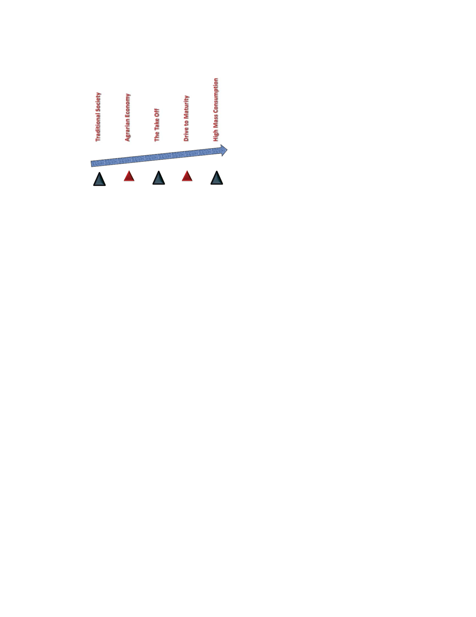
63
Figure 17. Rostovian Take-Off Model
These behaviors are 1) the traditional society, 2) the preconditions for takeoff, 3)
the takeoff, 4) the drive to maturity, and 5) the age of high mass consumption (Rostow,
1960). These observations are worthy and still stand true today 50 years later. In an
effort to plead the case for capitalism, however he went as far as saying one step needs to
happen before the next, eventually drawing a lot of criticism. Rostow focused on
financial capital, through mechanisms like foreign direct investment (FDI), to promote
the next level of development. Rostow included measurements that may not be universal,
like the Drive to Maturity stage comes about 60 years after the take-off (Rostow, 1960).
While this may very well be an observation he had at the time for some of the Nations he
was looking at, we know that time is relative and not all countries will follow this
measurement. This does not mean that the behavior classification is flawed, just some of
the measurements. While this has been shown to have significant flaws from a cause-
effect perspective, his classifications of behavior are still valid observations. Even by
today’s international organization model standards that only use three or four categories,
the five distinct behaviors used by Rostow can really divide up a large data pool for more
specific observation and may still be used today with modifications.

64
The other criticism with the take-off model is that, while it is the most popular
linear economic growth model, it does not account for negative growth. If a nation
achieves one level, can it only go back to the previous level, say, in the negative growth
years of Eastern Europe when the U.S.S.R. dissolved? With only two directions to go
(i.e., up or down), the model did not maintain popularity with researchers. If some of his
assumptions are removed, much can be added to this material, especially the distinct
behavior groups. I used his observations and overlaid them into the new model, one that
is not linear and one that accounts for both positive and negative growth. Rostow’s
(1960) model is a post war era model and it has a great foundation in behavior. It has
been selected for this reason and will be used in comparison to the non-linear behavior
international economic development growth path model.
Era 3: International organization era (1990s, 2000s, and 2010s)
Returning to the comparison to Piaget, the international organization era models
would likely fall under the concrete operational stage, the third stage of development. It
identifies what they call elementary logic of classes and relations (Piaget, 1964). The
economic models construct numbers, spatial temporal operations in the immediate
neighborhood with emphasis on agreed upon classifications. It does not seem that we
have gotten to the point where the economic growth models have evolved past this stage,
as we certainly do not agree upon classifications and are focused on local economics
instead of the economics of the whole global system. While advances are being made
and improvements are being achieved, it should be fair to say we are in the concrete
operational stage. The third stage will end with successive inclusions. The fourth stage,

65
the formal operational stage (Piaget, 1964), will come in the future when the economic
models involve hypothetic-deductive operations. Thus, as best we can determine,
economic growth and economic development models are only in stage three out of four,
indicating the nascence of the discipline.
Figure 18. International Organization Model Era.
Nielsen authored an IMF working paper titled “Classifications of Countries
Based on Their Level of Development: How it is Done and How it Could be Done” in
February of 2011. The paper outlines the dominant models used today by influential
international organizations, specifically model #8: the United Nations Development
Program (UNDP), model #9: the World Bank (WB), and model #10: the International
Monetary Fund (IMF), through their sheer size and dominant financial impact on
communities (see Figure 18). Essentially, Nielsen (2011) outlines the history and
development of the models most often used today to define international development of
nations. The political nature of each group, however, determines the outcome of these
models. This does not dampen the wide use and reliance on these models today. It
should be noted that the international development community is usually tied to the UN,
WB, and IMF. The relation of these international organizations and dominance in
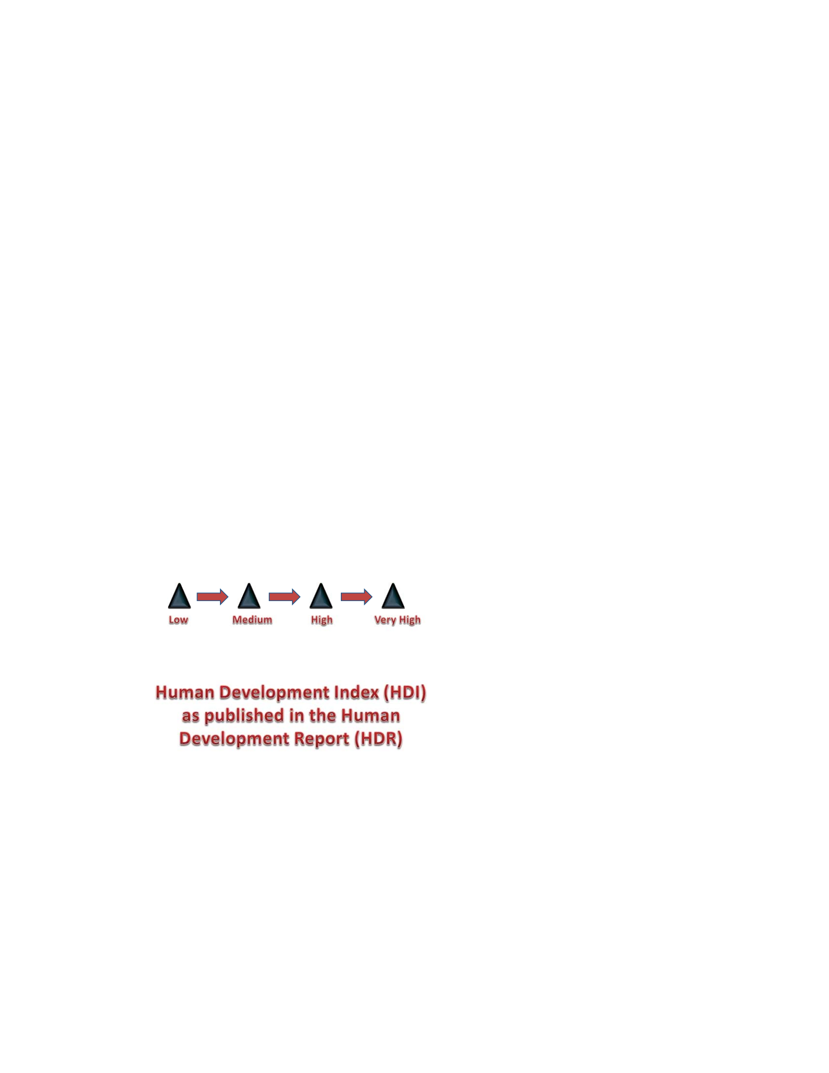
66
development literature significantly impacts the lens on the economic discipline, both
socially and academically.
Model 8: United Nations Model
“Where exactly to draw the line between developing and developed countries is
not obvious, and this may explain the absence of a generally agreed criterion,” Nielsen
(2011, p. 3) writes. Nielsen (2011) goes on, “This could suggest that a
developing/developed country dichotomy is too restrictive and that a classification
system with more than two categories could better capture the diversity in development
outcomes across countries” (p. 3). Nielsen identified shortcomings in the current
international organization models. The new behavioral international economic
development growth path study will use nine classifications in the model.
Figure 19. United Nations Model.
Historically, Nielsen (2011) identifies a landslide of literature that was content
with a two-classification model, “poor/rich, backward/advanced,
underdeveloped/developed, North/South, late-comers/pioneers, Third World/First World,
and developing/industrialized” (p. 4). While the third world/first world model really has

67
three classifications, the significance of the statement echoes with truth: It is not that a
two-classification system cannot shed light and insight on a topic. However, for models
to mature, sometimes they need to become more complex.
Sen and Mahbub ul Haq are credited for the UN model and for advancements in
what are now labeled human development factors. Sen, in a Nobel Prize Lecture, credits
Mahbub ul Haq as “the United Nations Development Programme (UNDP) has made
systematic use of a particular type of informational broadening to make comparisons
based on observed features of living conditions (Reported in UNDP, Human
Development Reports)” (Sen, 1998, p. 193).
“The rise of the South is radically reshaping the world of the 21st century, with
developing nations driving economic growth,” starts the 2013 Human Development
Report. It continues, “Lifting hundreds of millions of people from poverty, and
propelling billions more into a new global middle class, says the United Nations
Development Programme” (UNDP, 2013). This new trend is captured in an elaborate
research report model that was started in 1990 by the UNDP. The goal of this model was
to bring human capital development to the forefront. Mayer-Foulkes writes in 2010 in a
UNDP human development reports research paper, “Two decades of empirical
investigations left behind long-held views that economic growth consisted fundamentally
of a process of capital accumulation, finding that human capital, technology, institutions
and economic geography to be essential components of the process” (p. 2). Mayer-
Foulkes continues, “The main debate, nevertheless, is to what extent the growth process
generated by markets is sufficient to bring about economic development, and where not,

68
what the most effective complementary policies can be” (2010, p. 2). Mayer-Foulkes
also adds, “What these studies show is that economic and human developments are
complex processes with historical, political, economic, institutional and geographical
determinants that do not conform to some simple linear model” (Mayer-Foulkes, 2010, p.
3). Molina & Purser contribute add to the discussion when they contribute:
The main feature revealed by the descriptive analysis is that Human
Development, as well as its determinants, follow a series of superposed transitions
that first take off with increasing divergence and then converge to a higher
equilibrium. This very fundamental feature of development is almost completely
missing in most theoretical models on economic growth. It could be said that
vicious cycles keep transitions from beginning. Once they begin, they are
characterized by virtuous cycles that reach a higher equilibrium. The Human
Development Report is published once a year and outlines what is called the
Human Development Index, which is made up from a measurement of 22%
(weight) literacy rates, 11% gross education enrollment rates, 33% life expectancy
rates, and 33% GDP per capita. The scale is zero on the low side, and one on the
high, indicating better human development. (Molina & Purser, 2010, p. 4)
The UN can also be credited with the commonly used classification identified as
least developed countries (LDCs). As Nielson (2011) points out, the general assembly
never established what can be labeled as development taxonomy.
Model 9: World Bank Model
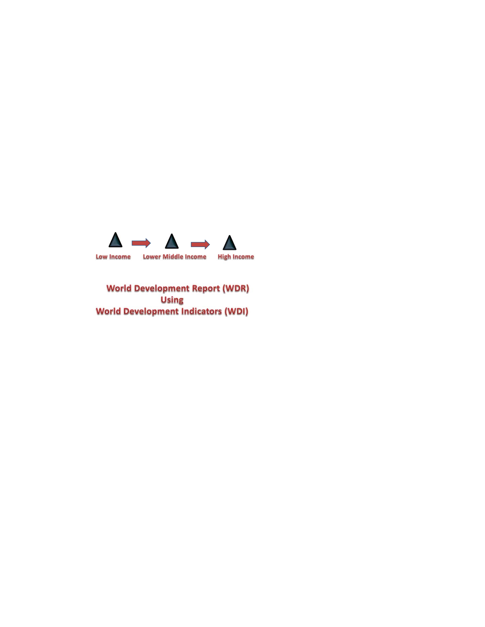
69
The WB model is based on absolute measures, meaning that a country either fits
into the category or doesn’t. The labels used, however, are relative: high, middle, and
low which allude to a division of statistics divided into thirds. This is not the case for the
WB, as the labels do not match the criteria evenly. It should be noted that the model has
changed over the last several decades. Currently, there are three indicator classifications:
low income, lower middle income, and high income.
Figure 20. World Bank Model.
The WB model is set up for a specific purpose: as a tool to help lend money. The
International Bank for Reconstruction and Development (IBRD) lends money to eligible
borrowers. This system is seen as a political model, which means it is based less on
scientific labeling but need/capacity or worthiness. While some nations may be
deserving of funding, if they are out of political favor, they may not qualify and put in a
different classification. It may seem peculiar to include non-scientific models in this
literature review; however, the WB has a significant research database and prominent
presence in research today. The World Development Indicators are a staple in modern
research. These are used and published in the World Development Report (WDR), which
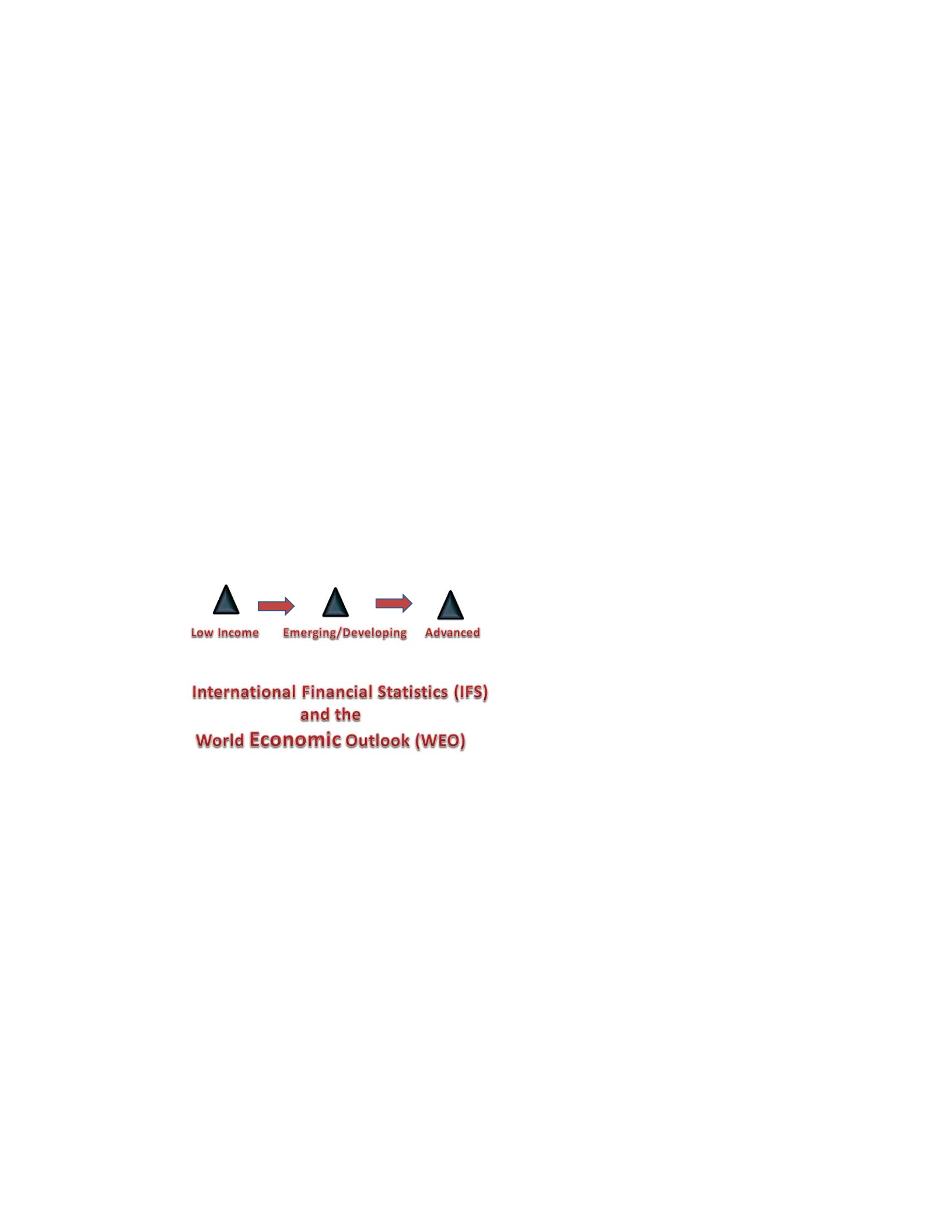
70
is another yearly publication. The visibility the WDR gets is impressive, but the
requirements to help lenders lend is paramount. Because of this important need, very
detailed information is collected. It is, therefore, an important source of information and
should be seen as a significant model in economic growth and economic development
research.
The WB has a financing arm called the International Development Association
or IDA. There are two primary tiers within the IDA, donors and borrowers, referred to as
Part 1 and Part 2. The lending threshold has changed over the years. This model should
be seen as a political tool, and deserves to be mentioned as a dominant model.
Figure 21. International Monetary Fund (IMP) Model.
Model 10: International Monetary Fund Model
The IMF model uses a simple three-classification approach. It is used as a
system to identify who may be eligible for loans. It is not based on a scientific method,
but a political and, more specifically, business method. The insight in this model is
similar to the other models in the international organization taxonomy theory collection.
Nielson (2011) breaks down the IMF country classification system, stating that

71
“operational policies related to financial assistance, surveillance, and technical assistance
did not discriminate among members based on their level of development for the first
three decades of the Fund’s existence” (p. 14).
Literature Review Conclusion
This literature review has identified 10 economic growth and development models
that have significantly impacted the academic discipline of international economics. I
have reviewed three eras of models and research. The first era highlighted models that
focused on productivity, industrialization, savings rates, and technology. The second era
of models focused on endogenous growth and looked within the national system for
answers. The third era is dominated by international organizations and their influence on
national systems in data collection and analysis. The underpinnings of global events
dominate each era. As we would expect in the economics field, most of the models used
are quantitative studies. In the first two eras, the World War Era and the Post War Era,
economic growth, math-centric, quantitative prediction models dominated research. In
the International Organization Era, development economics, human development
indicators, and qualitative models dominate research.
Economic Nobel Laureates Stiglitz (2001) and Ostrom (2009) identify a need for
new behavior models in economics to further the understanding of economic growth and,
specifically, development economics. The goal is to identify like development growth
paths or clusters. We may benefit from studying like groups and the behavior of these
new groups. The paradigm of looking at nation states as 1st world (post industrialized),

72
2nd world (industrializing), and 3rd world (agrarian and poor) is simply too vague and
broad to get specific insight and theoretical perspective in detail. A study that uses more
classification labels can help provide additional insight on this identified literature gap,
providing social benefit to public administrators with a new tool to help make better
management decisions.

73
Chapter 3: Research Method
Introduction to the BIED-GPM Design
I built upon the traditional linear growth (3 stages) model and the Rostovian (5
stage) Take Off model using the grounded theory Constant Comparison Method of
Strauss and Glaser (1967) and the structured coding procedures for data analysis from
Strauss and Corbin (1990). Glaser and Strauss wrote a ground-breaking book titled The
Discovery of Grounded Theory: Strategies for Qualitative Research in 1967. Glaser and
Strauss believe that grounded theory can promote relevant theory from quantitative data
and devote an entire chapter to it called, “Theoretical Elaborations of Quantitative Data.”
(p. 185). In this study I take quantitative data, as defined in the sub chapter titled
secondary analysis of quantitative data (p.185) through the 3 defined coding processes to
build a Conditional Matrix. Observe the behavior of the new stages of nonlinear growth
with qualitative methods until patterns arise. Grounded theory allows for both
quantitative and qualitative analysis, it, therefore, aligns well with this study. (Glaser &
Strauss, 1967, p. 1).
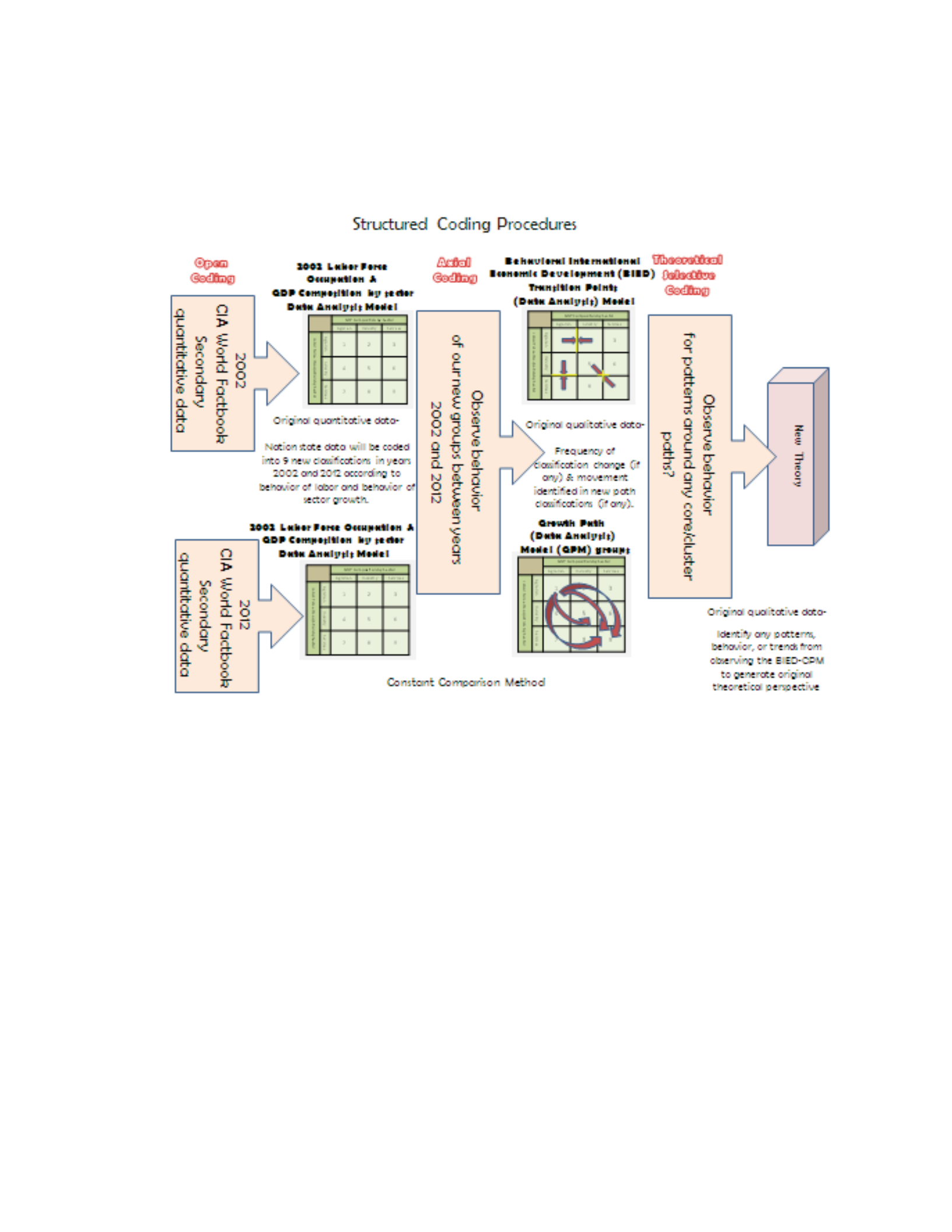
74
Figure 22. Grounded Theory Structured Coding Procedures.
The decision to use a sociology research method in an economic discussion is not
common. It is, however, an appropriate method for this research project. The current
paradigm with economic models leans heavily on quantitative methodology. Bitsch
(Bitsch, 2005) identifies that “qualitative research as understood in other social sciences
is virtually nonexistent in the American Journal of Agricultural Economics (AJAE).”
(p.75) Also, as nine classifications will be created (more than twice as many as most
models) in order to get a more specific picture as to what might be happening in the labor
sector. Strauss and Corbin’s (1990) work promotes grounded theory, “One does not
begin with a theory, then prove it” (p22). Grounded theory was chosen for its fluid and

75
open approach to theoretical conceptualization (Glaser & Strauss, 1967). Glaser and
Strauss (1967) go on to identify that grounded theory should provide perspective on
behavior.
Strauss and Corbin (1990) have put together a good set of procedures to help
guide a grounded theory study. They emphasize setting up structured coding procedures
to facilitate a research design. Unlike the Glaser approach that promotes an open slate
before the study to capture concepts inductively.
The role of the researcher is to design a secondary study from both the 2002 and
2012 CIA World Factbook. This provided a decade of data movement to review and new
classifications to observe. Since this is a path behavior study, the nonlinear movement
was built into the design to avoid some of the criticism found in the Rostovian Take off
model. This accommodates both positive and negative growth. Both a conditional
matrix was used as well as a conditional path.
GDP Composition by Sector
Agrarian Industry Services
Labor Force Occupation by Sector
Agrarian
123
Industry
456
Services
789
Figure 23. The Behavioral International Economic Development (BIED) Conditional Matrix Growth Path
Model.
Using the typical indicator of GDP by sector to help measure the growth of the
financial capital sector along with the new behavior indicator of labor force occupation

76
by sector to create a grid matrix, nine distinct classifications were created to help manage
the data set (see Figure 23). With GDP composition by sector on the top and labor force
occupation by sector on the side, both indicators help create a more specific look at the
CIA World Factbook data sets. All nations identified in the CIA World Factbook were
considered. If it could be determined what the majority GDP composition by sector is,
then it was used. If the majority labor force occupation by sector could be determined,
then it was used. Simple majority was used for this study: Whichever one of the three
has the largest percent was considered to dominant behavior of that society and therefore
was used in the model. The largest sectors, for the purpose of this study, will represent
the dominant classification in the new model.
Figure 3 showed two examples of how China could be labeled when GDP by
sector and Labor Force Occupation by sector were used independent from each other.
When we use both indicators together in figure 23, China’s GDP by Sector is (Agrarian-
9.60%, Industry-46.80%, & Services-43.60%) has Industry as the dominate sector.
China’s Labor Force by Occupation Model is (Agrarian- 38.10%, Industry-27.80%, &
Services-34.10%) or an Agrarian dominated labor force. Since the labor force is agrarian
and the GDP is industrial, these two indicators intersect in box 2 of the new BIED-GPM.
This example allows us to classify each nation state to see if it helps to get a more
detailed picture of what is happening. It also allows us a scientific way of measuring
paths and routes taken over time, which should be helpful in any analysis comparisons.
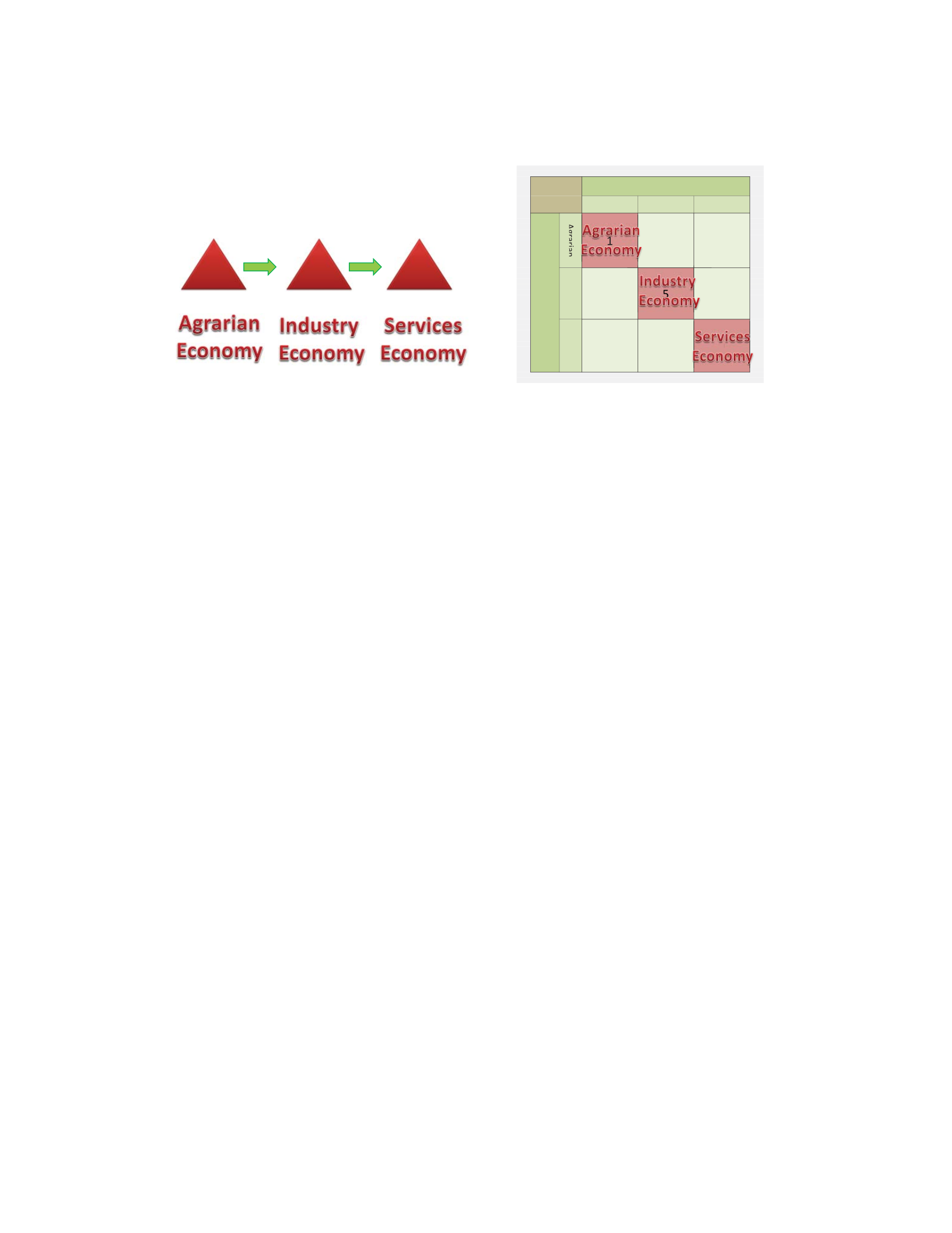
77
Vs.
GDP Composition by Sector
Agrarian Industry Services
Labor Force Occupation by Sector
Agrarian
123
Industry
456
Services
789
Agrarian
1
5
5
5
5
5
5
5
5
5
5
5
5
5
5
5
5
5
5
5
5
5
5
5
5
5
5
5
5
5
5
5
5
5
5
5
5
9
9
9
9
9
Figure 24. Traditional Linear Growth Model Embedded in the BIED-GPM.
Figure 24 demonstrates how Figure 1 (the traditional linear growth model) might
look when added into the new BIED-GPM. The traditional linear path would move from
classification box 1 (agrarian) to box 5 (Industry,) and then to box 9 (Services). Having
six additional classifications should help to define a society’s behavior in more depth.
This new model also allows for negative and nonlinear movement. It also allows
researchers the opportunity to systematically look at economic paths. How does one
system move between these different classifications? The outcome is that by studying
any changes of classification movement, that policy makers might be able to better
prepare for what is most likely the next dominant behavior of a particular society. This
behavior has its own set of concerns, priorities, and considerations. This study does not
get into depth on the concerns, priorities, and considerations within each stage, but will
attempt to assess whether the data and analysis of such a lens contributes significant
insight into the relations identified. If significant insight is possible, then further
clarification research might be ideal for future research. Grounded Theory allows the
inductive process to happen as many times as needed, until patterns surface.
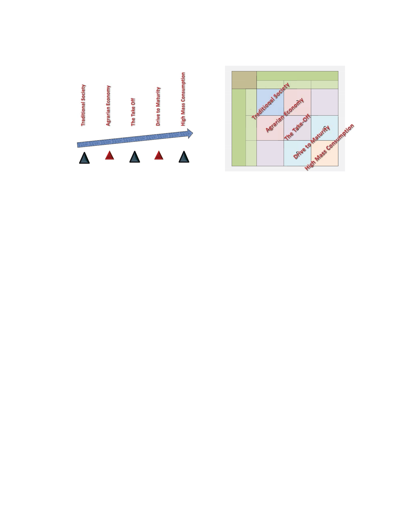
78
Vs
GDP Composition by Sector
Agrarian Industry Services
Labor Force Occupation by Sector
Agrarian
123
Industry
456
Services
789
GDP
Compo
sit
Ag
rar
i
a
n
I
n
d
u
Ag
rar
i
a
n
Ind
u
2
2
2
2
2
2
2
2
2
2
2
2
2
2
2
2
2
2
2
2
2
2
2
2
2
2
2
2
2
2
2
2
2
2
2
2
2
2
2
2
2
2
2
2
2
2
2
2
2
2
2
2
2
2
2
2
2
2
2
2
2
2
2
2
2
2
2
2
2
2
2
2
2
2
2
2
2
2
2
2
2
2
2
2
2
2
2
2
2
2
2
2
2
2
2
2
2
2
2
2
2
2
2
2
2
2
2
2
2
2
2
2
2
2
2
2
2
2
2
2
2
2
2
2
2
2
2
2
2
2
2
2
2
2
2
2
2
2
2
2
2
2
2
4
4
4
4
4
4
4
4
4
4
4
4
4
4
4
4
4
4
4
4
4
4
4
4
4
4
4
4
4
4
4
4
4
4
4
4
4
4
4
4
4
4
4
4
4
4
4
4
4
4
4
4
4
4
4
4
4
4
4
4
4
4
4
4
4
4
4
4
4
4
4
4
4
4
4
4
4
4
4
4
4
4
4
4
4
4
4
4
4
4
4
4
4
4
4
4
4
4
4
4
4
4
4
4
4
4
4
4
4
4
4
4
4
4
4
4
4
4
4
4
4
4
4
4
4
4
4
4
4
4
4
4
4
4
4
4
4
4
4
4
4
4
4
4
4
4
4
4
4
4
4
4
4
4
4
4
4
4
4
4
4
4
4
4
4
4
1
1
1
1
1
1
1
1
1
1
1
1
1
1
1
1
1
1
1
1
1
1
1
1
1
1
1
1
1
1
1
1
1
1
1
1
1
1
1
1
1
1
1
1
1
1
1
1
1
1
1
1
1
1
1
1
1
1
1
1
1
1
1
1
1
1
1
1
1
1
1
1
1
1
1
1
1
1
1
1
1
1
1
1
1
1
1
1
1
1
1
1
1
1
1
1
1
1
1
1
1
1
1
1
1
1
1
1
2
2
2
2
2
2
2
2
2
2
2
2
2
2
2
2
2
2
2
2
2
2
2
2
2
2
2
2
2
2
2
2
2
2
2
2
2
2
2
2
2
4
4
4
4
4
4
4
4
4
4
4
4
4
4
4
4
4
4
4
4
4
4
4
4
4
4
4
4
4
4
4
4
4
4
4
4
4
4
4
4
4
4
4
4
4
4
4
4
4
4
4
4
4
4
4
4
4
4
4
4
4
4
4
4
4
4
4
4
4
8
8
8
8
8
8
8
8
8
8
8
8
8
8
8
8
8
8
8
8
8
8
8
8
8
8
8
8
8
8
8
8
8
8
8
8
8
8
8
8
8
8
8
8
8
8
8
8
8
8
8
8
8
8
8
8
8
8
8
8
8
8
8
8
8
8
8
8
8
8
8
8
8
8
8
8
8
8
8
8
8
8
8
8
8
8
8
8
8
8
8
8
8
8
8
8
8
8
8
8
8
8
8
8
8
8
8
8
8
8
8
8
8
8
8
8
8
8
8
8
8
8
8
8
8
8
8
8
8
8
8
8
8
8
8
8
8
8
8
8
8
8
8
8
8
8
8
8
8
8
8
8
8
8
55
5
5
55
5
5
5
5
5
5
5
5
5
5
5
5
5
5
5
5
5
5
5
5
5
5
5
5
5
5
5
5
5
5
5
5
5
5
5
5
5
5
5
5
5
5
5
5
5
5
5
5
5
5
5
5
5
5
5
5
5
5
5
5
5
5
5
5
5
5
5
5
5
5
5
5
5
5
5
5
5
5
5
5
5
5
5
5
5
5
5
5
5
5
5
5
5
5
5
5
5
5
5
5
5
5
5
5
5
5
5
5
5
5
5
5
5
5
5
5
5
5
5
5
5
5
5
5
5
5
5
5
5
5
5
5
6
6
6
6
6
6
6
6
6
6
6
6
6
6
6
6
6
6
6
6
6
6
6
6
6
6
6
6
6
6
6
6
6
6
6
6
6
6
6
6
6
6
6
6
6
6
6
6
6
6
6
6
6
6
6
6
6
6
6
6
6
6
6
6
6
6
6
6
6
6
6
6
6
6
6
6
6
6
6
6
6
6
6
6
6
6
6
6
6
6
6
6
6
6
6
6
6
6
6
6
6
6
6
6
6
6
6
6
6
6
6
6
6
6
6
6
6
6
6
6
6
6
6
6
6
6
6
6
6
6
6
6
8
8
8
8
8
8
8
8
8
8
8
8
8
8
8
8
8
8
8
8
8
8
8
8
8
8
8
8
8
8
8
8
8
8
8
8
8
8
8
8
8
8
8
8
8
8
8
8
8
9
9
9
9
9
9
9
9
9
9
9
9
9
9
9
9
9
9
9
9
9
9
9
9
9
9
9
9
9
9
9
9
9
9
9
9
9
9
9
9
9
9
9
9
9
9
9
9
9
9
9
9
9
9
9
9
9
9
9
9
9
9
9
9
9
9
9
9
9
9
9
9
9
9
9
9
9
9
9
9
9
9
9
9
9
9
9
9
9
9
9
9
9
9
9
9
9
9
9
9
9
9
9
9
9
9
9
9
9
9
9
9
9
9
9
9
9
9
9
9
9
9
9
9
9
9
9
9
9
5
5
5
5
5
5
5
5
5
5
5
5
5
5
5
5
5
5
5
5
5
5
5
5
5
5
5
5
5
5
Figure 25. Rostovian Take-Off Model Inside The BIED-GPM.
Figure 25 displays the Rostovian take-off model when identified within the new
behavioral international (nonlinear) economic development growth path model.
Classification box 1 identifies Rostow’s traditional society. Boxes 2 and 4 identify the
agrarian economy. Boxes 3, 5, and 7 identify the take-off stage. Boxes 6 and 8 identify
the drive to maturity stage. Finally, box 9 identifies the high mass consumption stage.
In 1961, Ohlin wrote “Reflections on the Rostow Doctrine;” with further dissent
by Itagaki (1963) in “Criticism of Rostow’s Stage Approach: The concepts of Stage,
System, and Type,”noting that “It is only in the third stage (“take off”) and the fifth stage
(“high mass-consumption”) that Rostow’s leading sectors emerge” (Itagaki, 1963, p. 5).
What Ohlin and Itagaki identify is that the traditional society stage, the take-off stage,
and the high mass consumption stage (stages 1, 3, and 5) are primary stages, while the
agrarian economy stage and drive to maturity stage are more transitional in nature. While
neither had the benefit of the behavior international economic (nonlinear) development
growth path model conditional matrix (BIED-GPM), we can more clearly conceptualize
what each was describing (in Figure 25). The primary stages are agrarian GDP and

79
agrarian-dominated labor force occupation by sector (stage 1), industry GDP and
industry-dominated labor force by sector (stage 5), and services GDP and services-
dominated labor force occupation by sector (stage 9). This can be identified by the
earliest observations and classifications in the traditional linear growth model. While
Ohlin (1961) and Itagaki (1963) may have observed a weaker relationship in the second
and fourth stages, Rostow’s (1961) seminal contribution is identifying additional
classifications and ultimately behavior observations to grow the body of understanding in
the first place. Rostow’s attempt to define each stage at the time was actually an attempt
to classify the observed behavior. The attempt used stretching assumptions and flawed
measurements which led too much of the criticism of the model. The original behavior
observations, however, are strong.
When actual behavior is used and classified, a different picture is possible. Also
having four extra classifications helps add depth to the five observed categories in the
Rostow model. The thought is that behavior dominates a society. If the majority of
people in a society or “system” are making a living doing one type of occupation
compared to another, then it is the dominant behavior that is driving the economy. The
public policy in a system that is made up of farmers is focused on one set of issues, while
a system that is made up of factory workers has a different set of issues. It should be the
behavior that should define the classifications along with GDP (a measure of the success
of each behavior). Together, these two indicators, GDP composition by sector and labor
force occupation by sector, help to show the dominant behavior and relative return on
behavior, which should be useful in theory development. Itagaki (1963) calls for “a fresh
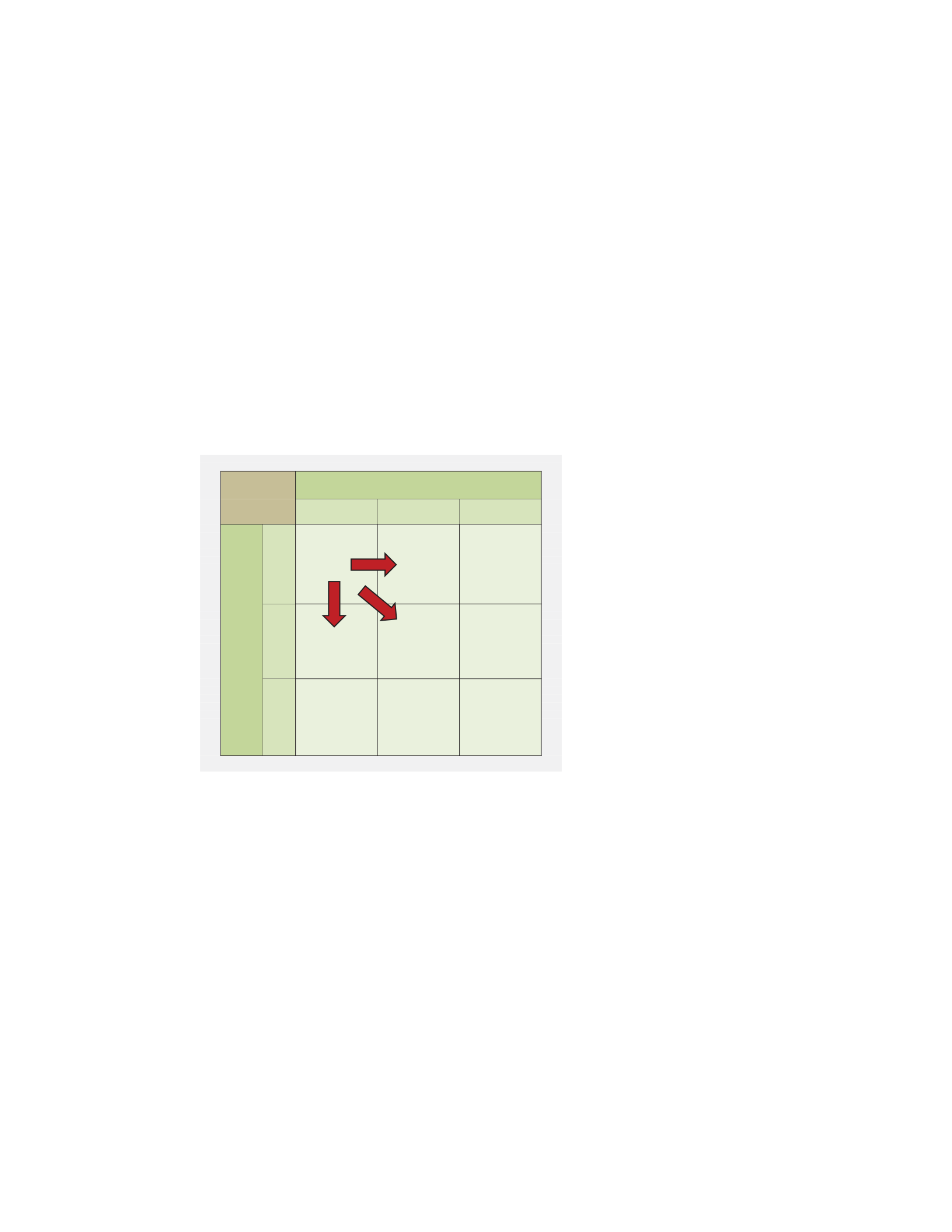
80
approach to the stage theory, in order to unify the knowledge of theory, history and
policy by distinguishing and relating at the same time the key concepts of ‘stage,’
‘phase,’ ‘system,’ ‘type,’ ‘policy,’ and ‘strategy’” (p. 17).
Using the previously discussed traditional linear growth model (see Figure 1), we
know that most nations start in classification 1, an agrarian economy. When they
industrialize they will move out of classification 1. There are only three options:
classifications 2, 4, or 5 (see Figure 26).
GDP Composition by Sector
Agrarian Industry Services
Labor Force Occupation by Sector
Agrarian
123
Industry
456
Services
789
Figure 26. Corners Only Have Three Path Options.
After industrialization, we know that a move to the service sector is likely if using
an upward growth trend. This move would depend on what category dominates during
the industrialization phase. What this model does is capture the growth, either positive or
negative, in the financial sector as dominated in GDP composition by sector. It also
includes the behavior of individuals to choose a job in a specific sector. Assuming
people vote in opposition and decide what job to participate in, and then a conscious
choice is made to be in an agrarian, industry, or services occupation. Using the belief
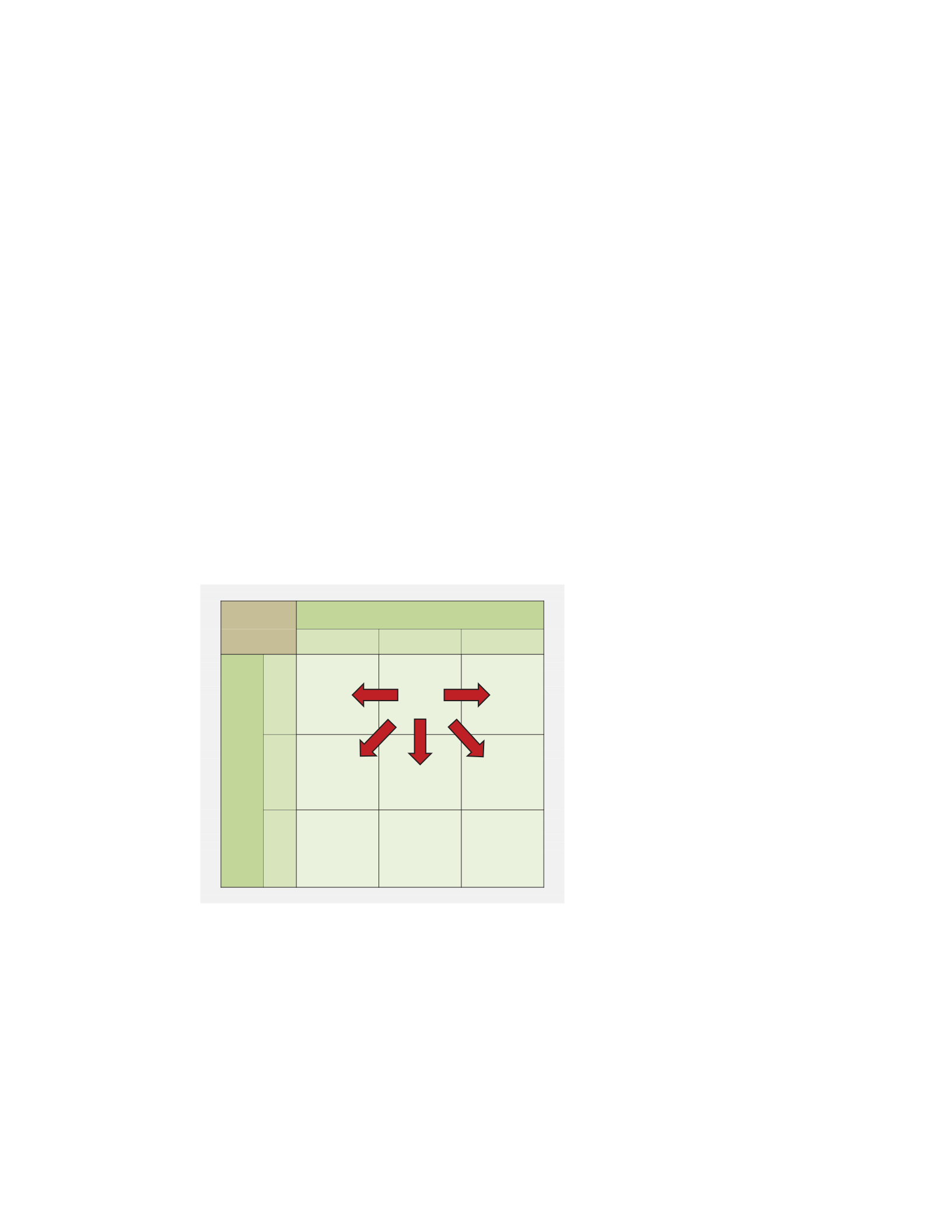
81
that behavior is a better matrix of what is important in policy and administrative
considerations, but still identifying that the actual increase in financial capital grows the
economy triangle, the combination of both indicators should provide considerable depth
when we get to the analysis stage in the research.
The outside middle classifications (2, 4, 6, and 8) have five options (see Figure
27). This is considerably more than the corners and will impact probability during path
analysis. Each classification allows for the reality of positive, as well as negative growth.
This is a distinction from several models that only accommodate positive growth.
Negative growth happens and the model should accommodate what is actually
happening.
GDP Composition by Sector
Agrarian Industry Services
Labor Force Occupation by Sector
Agrarian
123
Industry
456
Services
789
Figure 27. Outside Middle Classifications Have Five Options.
Finally, the center of the model, classification 5, has eight different directions;
giving it the most options of any of the classifications (see Figure 28). This gives a
society with the majority of its money coming in from the industry sector and when the
majority of their labor force is earning a living in industry, the most options.
82
GDP Composition by Sector
Agrarian Industry Services
Labor Force Occupation by Sector
Agrarian
123
Industry
456
Services
789
Figure 28. The Center Has The Most Options With Eight.
There are several paths that are possible, but the most common path is not known
at this time. We do know that the corners (1, 3, 7, and 9) have the fewest options (i.e.,
only three bordering classifications). Category 5 has the most options, being eight.
While there is some insight into this model based on probability, there should not be any
bias. The data will fall where it may. Once the data from 2002 and 2012 is collected, we
should be able to see what movement has happened in the last decade, if any. This will
give us an indication where the current trends may be for this ten year period. Please see
Figure 29 for path options (these are only examples of possible movement/insight from
the BIED-GPM).
83
GDP Composition by Sector
Agrarian Industry Services
Labor Force Occupation by Sector
Agrarian
123
Industry
456
Services
789
Figure 29. A Few Path Analysis Examples.
Figure 29 displays four examples of paths. One follows a path of 1, 2, 3, 6, and 9.
One follows a path of 1, 2, 5, 6, and 9. Another path is 1, 4, 5 and the last example path
is 1, 4, 7, 8, and 9. If enough data is collected, a nation could be tracked and could help
determine the most common behavioral economic growth path. This would give public
policy and public administrators some likely and probable paths to plan towards, or
perhaps even attempt to prevent or avoid. This model will accommodate both positive
growth as well as negative growth. It is not linear, but provides a new observable
dimension and should provide new insight into the economic growth literature,
development economics literature, and particularly to the behavior economics literature.
Follow-up research may examine to specific patterns. Specifically, what
behaviors are commonly found in one path compared to the behaviors of another path?
Using both behavior and path analysis can broaden the understanding of these economic
relationships.
Researcher’s Role

84
The researcher will use the CIA World Factbook data from 2002 and 2012. All
profiles in each publication were reviewed to determine if enough information can
determine which sector is the largest. The 2002 Factbook has 268 profiles, while the
2012 Factbook has 257. The sample size for this study uses all 525 nation state profiles
to get the broadest insight possible. Some of these profiles are not actual nation states but
collectives like “the world”. I used all entries to determine if they had enough data to
evaluate. The two indicators that I used can be found in the Central Intelligence Agency
(CIA) in the World Factbook, GDP composition by sector and labor force occupation by
sector. Each of these indicators is found in the economy section of the profile. With two
indicators and three measurements in each (that of agrarian, industry, & services) a total
of six statistics per nation state will be considered. Any profile that does not clearly
indicate all three categories for each indicator in agrarian, industry, and services will not
be able to move to the next round of evaluation in the grounded theory process. Only
profiles that had collected a clear advantage from all six categories will be used in this
study and added to the new conditional matrix model.
This study utilizes secondary data and thus, only the statistical information found
in the 2002 and 2012 CIA World Factbooks will be used (CIA, 2011). Ethical protection
has been considered and every effort was made to be transparent in the data collection,
assembly into the new model, and analysis as possible.
Emerging Concerns
There is a lot of material to cover in an international study this large. With 525
samples to review, qualify, build in the new model, validate, compare the last decade’s

85
movement, and interpret, many emerging concerns are possible. The priority for this
study was to cycle 10 years of data through this new model to see if the international
economic development growth path behavioral model can provide substantial insight for
comparative purposes. Follow-up research may add to the depth of this model by
including more years to provide a longer path perspective. Also, once enough data is
input, a better grasp of the common path routes can be considered through basic
probability reviews. Unlike the international organization taxonomy theory, which is
political in nature, this behavioral approach is based in scientific principles, allowing for
a more stable foundation.
Context
The concept of using a sociology method (i.e., grounded theory) to review and
study the math-centric and dominated discipline of economics is unique. When most
economic studies are quantitative, a need for qualitative research exists. Several
economists have identified a need for a new approach of looking at economic interaction.
The context of this study is an attempt to bridge gaps in previous models in order to
account for positive, as well as negative economic, growth. One of the unique principles
of this new model is its ability to account for lateral shifts, forward progress, and negative
cycles. Its foundation is pinned to behavior. Behavior, which is considered to be the best
indicator for policy and administration professionals, is what seems to be missing from
the economic discipline as a whole until now.
Participant Criteria

86
Because this is a secondary study, the participants that are used in the CIA World
Factbook will be nation state entries. As many profiles will be used as possible, as long
as there has been enough data collected to determine the largest percentage agrarian,
industry, or services sector for each of the two indicators. Whatever indicator that has the
highest percentage will be used and considered to be the dominate behavior for both
indicators. The original data collection was done on a massive scale. It can be more
clearly defined from the 2012 Factbook introduction:
The World Factbook is prepared by the Central Intelligence Agency for the use of
US Government officials, and the style, format, coverage, and content are
designed to meet their specific requirements. Information is provided by
Antarctic Information Program (National Science Foundation), Armed Forces
Medical Intelligence Center (Department of Defense), Bureau of the Census
(Department of Commerce), Bureau of Labor Statistics (Department of Labor),
Central Intelligence Agency, Council of Managers of National Antarctic
Programs, Defense Intelligence Agency (Department of Defense), Department of
Energy, Department of State, Fish and Wildlife Service (Department of the
Interior), Maritime Administration (Department of Transportation), National
Geospatial-Intelligence Agency (Department of Defense), Naval Facilities
Engineering Command (Department of Defense), Office of Insular Affairs
(Department of the Interior), Office of Naval Intelligence (Department of
Defense), US Board on Geographic Names (Department of the Interior), US

87
Transportation Command (Department of Defense), Oil & Gas Journal, and other
Public and private sources. (CIA, 2011, p. v)
Model Indicators
There will be two indicators in this study. The first is a common economic
measurement, known as GDP broken into three sectors, agrarian, industry, and services.
The CIA World Factbook (2012) defines how they collected GDP and the methodology
used in their calculations of GDP:
In the Economy category, GDP dollar estimates for countries are reported both on
an official exchange rate (OER) and purchasing power parity (PPP) basis. Both
measures contain information that is useful to the reader. The PPP method
involves the use of standardized international dollar price weights, which are
applied to the quantities of final goods and services produced in a given economy.
The data derived from the PPP method probably provide the best available
starting point for comparisons of economic strength and well-being between
countries. In contrast, the currency exchange rate method involves a variety of
international and domestic financial forces that may not capture the value of
domestic output. Whereas PPP estimates for OECD countries are quite reliable,
PPP estimates for developing countries are often rough approximations. In
developing countries with weak currencies, the exchange rate estimate of GDP in
dollars is typically one-fourth to one-half the PPP estimate. Most of the GDP
estimates for developing countries are based on extrapolation of PPP numbers
published by the UN International Comparison Program (UNICP) and by

88
Professors Robert Summers and Alan Heston of the University of Pennsylvania
and their colleagues. GDP derived using the OER method should be used for the
purpose of calculating the stare of items such as exports, imports, military
expenditures, external debt, or the current account balance, because the dollar
values presented in the Factbook for these items have been converted at official
exchange rates, not at PPP. One should use the OER GDP figure to calculate the
proportion of, say, Chinese defense expenditures in GDP, because that share will
be the same as one calculated in local currency units. Comparison of OER GDP
with PPP GDP may also indicate whether a currency is over or under valued. If
OER GDP is smaller than PPP GDP, the official exchange rate may be
undervalued, and vice versa. However, there is no strong historical evidence that
market exchange rates move in the direction implied by the PPP rate, at least not
in the short or medium-term. (CIA, 2011, p. xi)
The GDP composition by sector (i.e., agrarian, industry, and services) is
the first indicator that will be used. It will be the quantifiable indicator to identify
the actual success of the profile economy. It will also capture the sector that is
dominated in each country. The second indicator that will be used is labor force
occupation by sector. This will be the qualitative indicator. It is also the
contribution to behavior and human development as recommended by Ostrom
(2009). Together these two indicators will fill the nine classifications of the new
BIED-GPM.
Coding Procedures

89
Strauss and Corbin’s (1991) guidelines were used in this study to inform the
method. Open coding will be used first. Open coding as defined by Strauss and Corbin
(1991) is “The process of breaking down, examining, comparing, conceptualizing, and
categorizing data” (p. 96). Here the models were identified and open coded, axial coding
came next. According to Strauss and Corbin (1991), axial coding is an opportunity to put
information back together in new classifications (p. 96).
A conditional matrix was used and conditional paths followed the open and axial
coding process. Strauss and Corbin (1991) identify conditional matrix as “an analytic
aid, a diagram useful for considering the wide range of conditions and consequences
related to the phenomenon under study. The matrix enables the analyst to both
distinguish and link levels of conditions and consequences” (p. 158). Following the
conditional matrix, a conditional path was used. Strauss and Corbin (1991) define this
step as “the tracking of an event, incident, or happening from action/interaction through
the various conditional and consequential levels, and vice versa, in order to directly link
them to a phenomenon” (p. 158).
2002 2012 Difference
GDP Composition by Sector
Agrarian Industry Services
Labor Force Occupation by Sector
Agrarian
123
Industry
456
Services
789
GDP Composition by Sector
Agrarian Industry Services
Labor Force Occupation by Sector
Agrarian
123
Industry
456
Services
789
GDP Composition by Sector
Agrarian Industry Services
Labor Force Occupation by Sector
Agrarian
123
Industry
456
Services
789
Figure 30. 2002 and 2012 Compared For Any Path Movement For This Decade.
90
Two data points were collected in this study, one in 2002 and the second in 2012.
A difference matrix was then created to identify any changes during this ten year period
to look at any trends that were visible (see Figure 30). The majority or dominant sector
for each indicator was put into the model and intersect in one of the nine classifications.
Now that the countries have been input for both years, an appendix includes each country
name in each of the nine classification boxes. To depict actual path movement, the
transition points (see Figure 31) were used to see what nations and what percentage of
collected states had movement. The transition points are any line or corner located inside
the model. Crossing a transition point indicates significant movement in a nation’s sector
GDP or a labor shift. Either of these two events indicates a stage change. When the open
coding was completed, there are now two snapshots. The axial coding began to capture
any movement between transition points and was identified in the movement difference
matrixes. The most common path is the transition point with the highest value. The line
or point that has been crossed the most will identify the most common system movement
path during this decade.
GDP Composition by Sector
Agrarian Industry Services
Labor Force Occupation by Sector
Agrarian
123
Industry
456
Services
789
Figure 31. Transition Points (12 lines and 4 corners = 16 points).

91
The model has nine nonlinear stages as follows:
x Classification (1) Agrarian GDP with Agrarian Labor
x Classification (2) Industry GDP with Agrarian Labor
x Classification (3) Services GDP with Agrarian Labor
x Classification (4) Agrarian GDP with Industry Labor
x Classification (5) Industry GDP with Industry Labor
x Classification (6) Services GDP with Industry Labor
x Classification (7) Agrarian GDP with Services Labor
x Classification (8) Industry GDP with Services Labor
x Classification (9) Services GDP with Services Labor
The model has 16 transition points between Classification stages. They are:
1. Between classification 1 & 2
2. Between classification 2 & 3
3. Between classification 4 & 5
4. Between classification 5 & 6
5. Between classification 7 & 8
6. Between classification 8 & 9
7. Between classification 1 & 4
8. Between classification 2 & 5
9. Between classification 3 & 6
10. Between classification 4 & 7
11. Between classification 5 & 8

92
12. Between classification 6 & 9
13. Between classification 1 & 5
14. Between classification 3 & 5
15. Between classification 7 & 5
16. Between classification 9 & 5
Strauss and Corbin (1990) define 7 criterion found in the Judging a Grounded
Theory Study, subchapter. (p253) This criterion helped to facilitate a proven technique
tied to the Strauss & Corbin Grounded Theory constant comparison method. The
criterion is:
x Criterion #1: How was the original sample selected? What grounds?
x Criterion #2: What major categories emerged?
x Criterion #3: What were some of the events, incidents, actions, and so on (as
indicators) that pointed to some of these major categories?
x Criterion #4: On the basis of what categories did theoretical sampling proceed?
That is, how did theoretical formulations guide some of the data collection? After
the theoretical sampling was done, how representative did these categories prove
to be?
x Criterion #5: What were some of the hypotheses pertaining to conceptual relations
(that is, among categories), and on what grounds were they formulated and tested?
x Criterion #6: Were there instances when hypotheses did not hold up against what
was actually seen? How were these discrepancies accounted for? How did they
affect the hypotheses?

93
x Criterion #7: How and why was the core category selected? Was this collection
sudden or gradual, difficult or easy? On what grounds were the final analytic
decisions made?
These seven criterions were used to empirically ground this research according to
Strauss & Corbin (1990) defined procedures.
Grounded Theory Method: (BIED-GPM)
The conclusion of this study is to further develop classifications of behavior by
nation state systems using two indicators, Gross Domestic Product by sector and Labor
Force by Occupation Sector. With a better understanding of past behavior and a broader
conceptualization of future options, this study identifies nonlinear movement as nations
develop. This should assist public administrators make better policies and contribute to a
social benefit in better analysis. The movement through “development stages” is actually
the study of group behavior. By using attributes of development economics and behavior
economics, synergies were found to further both disciplines.

94
Chapter 4: Research
Introduction
Using the Strauss and Corbin (1990) coding procedures for grounded theory
constant comparative method, this study used open coding, axial coding, and theoretical
selective coding. The open coding stage identified the CIA World Factbook nations in
2002 and 2012 (see Appendix B for 2002 and Appendix C for 2012). All nations were
put into a BIED-GPM to identify if they had enough indicator information to determine if
a dominate sub category (Agrarian, Industry, or Services) could be found in both
indicators, Gross Domestic Product Composition by Sector and Labor Force Occupation
by Sector. If a dominate sector was found in each sub category in both indicators, the
nation was assigned an axial coding number and was examined further in the axial coding
stage. If there was not enough information found in either the 2002 or 2012 CIA World
Factbooks, the nation was not reviewed further as identified in Appendix D: open coding
results.
The axial coding stage assigned each nation that had enough information on GDP
and Labor Force a Growth Path number. This number was found by putting each nation
into one of nine new classifications in the BIED-GPM for each year examined, 2002 and
2012. Once a determination could be made as to what classification each nation was in
during each year, the path was examined. The path number is the 2002 BIED-GPM
number followed by the 2012 BIED-GPM number. This combination of numbers creates
a sequence known as the BIED-GPM path number.

95
Finally, once each nation was reclassified into growth path numbers, the
Theoretical Selective Coding Stage put the newly identified paths into yet another
classification based on identified behavior. With this grounded theory process a wealth
of information was identified, reviewed, observed, classified, and new insight is now
possible.
Setting and Demographics
The setting of this study is grounded in new labels and observing the newly
labeled groups. If the data clearly indicates the dominant behavior in each indicator
(GDP composition by sector & Labor Force by Occupation) sub categories, agrarian,
industry, or services, it falls into one of nine classifications based on which indicator
most influences the system. If there was concern with the data collection computation,
the inquiry can be addressed with CIA Statistics managers. This study promotes a new
way of looking at international development and growth.
The demographics of this study were international nation state labels. While
these are political classifications and change from time to time, because they include
several territorial claim disputes, etc. International accepted boundary norms were used
as defined in the Factbook parameters. These norms should provide validity to the
categories used and support the new classifications built in this study. Individual
economic systems and nation-state systems are initially studied in this study. Once new
economic labels are identified, these new groups are studied.
Data Collection

96
The data collection was rigorous, by putting each nation state entry from both the
2002 and 2012 CIA World Factbooks into the BIED-GPM to identify if a 1-9 stage could
be identified in each year. Of 279 original open coded nation-state entries, 115 had
enough information to move into the axial coding stage. Appendix B shows the 2002
CIA World Factbook nations in new BIED classification stages, one through nine.
Appendix C shows the 2012 CIA World Factbook nations with new BIED classifications
stages. These new BIED Classification Stages identify the behavior of individual
decisions to work in the agrarian, industry, or services sectors. There are many factors
that go into a decision to work in one of these three sub categories, like potential income,
educations, availability, community prestige, as well as both short and long term
interests. These decisions are represented by the labor force occupation indicators. The
gross domestic product composition by sector behavior indirectly shows policy decisions
made by nation-state government economic systems. The decision making criteria of
individual economic systems and nation-state economic systems are made with both short
term and long term interests calculated ultimately impacting behavior.
Appendix D shows the outcome of the Open Coding stage. Of the 268 identified
nation states in the 2002 Factbook and 257 nation states in the 2012 Factbook (totally 279
different nations), 115 nation entries had enough data to clearly determine where the
dominant behavior of sector GDP was coming and from what sector the majority of the
working labor force was coming. These two indicators, when used together, help identify
one of nine new BIED classifications. When both indicators had enough information to
clearly determine each sector, they were combined in the growth path model to get a

97
cross classification or a combined GDP/Labor Force by sectors label known here as a
BIED-GPM classification stage.
Data Analysis-Open Coding
Open Coding was conducted by putting the available data found in both the 2002
and 2012 CIA World Factbooks into the matrix in Figure 32. The nine boxes represent a
new labeling system that helps track economic stage movement during this study when
multiple points are reviewed. For this study two points were reviewed, one in 2002 and
another in 2012. BIED-GPM stage one is an agrarian dominated GDP economy and an
agrarian dominated labor force economy. BIED-GPM stage five is an industry
dominated GDP economy and an industry dominated labor force economy, stages one,
five, and nine are considered prime stages because both the GDP and labor is the same
(agrarian-agrarian, industry-industry, or services-services). BIED-GPM stage nine is a
service dominated GDP economy and a service dominated labor force economy. The
stages in between are a combination of agrarian, industry, or service dominated GDP
economies and agrarian, industry, or services labor force dominated economies. Each
nation will get a new label that will include both the source of sector income and sector
labor in one easy BIED-GPM stage 1-9.

98
Figure 32. BIED-GPM Grounded Theory Non Linear Conditional Matrix.
A trend was identified only from the nations that had enough information in both
2002 and 2012 to clearly identify a BIED-GPM stage twice, showing two points to
determine a trend. If both stages were identified and given new labels then they were
included in the trend analysis. In 2002, 67 nations fell into the advanced economic stage
of having a GDP services dominated economy and a Labor Force by Occupation services
dominated working force or stage 9. In 2012 this number increased by 34 nations states
to 101. Open Coding Analysis showed the following information (see Figure 33), two of
the stages reduced (stage 1 and stage 3). During the ten years covered in this study, both
stage 1 and stage 3 lost nations. Three stages stayed the same, stage 4 (Agriculture GDP
& Industry Labor), stage 6 (Services GDP & Industry Labor), and stage 7 (Agriculture
GDP & Services Labor) with zero nation states. Ten nation states have moved into
Labor Force by Occupation
Grounded Theory Non Linear Conditional Matrix-
Behavioral International Economic Development (BIED)
Growth Path Model (GPM)
2
5
8
3
6
9
Industry Services
Agriculture Industry Services
Agriculture
1
4
7
Gross Domestic Product Composition by Sector
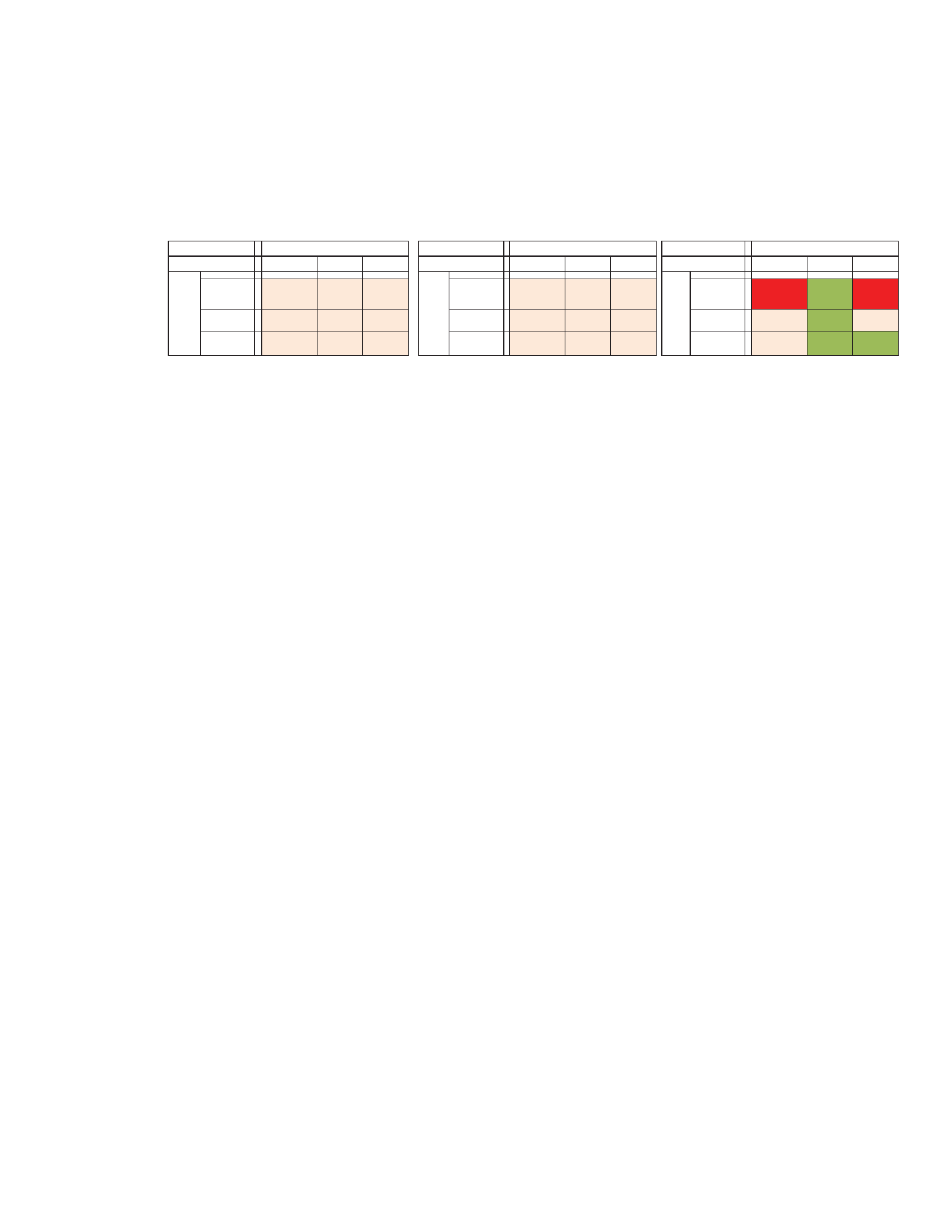
99
industry dominated GDP, stage 2 (Industry GDP & Agriculture Labor), stage 5 (Industry
GDP & Industry Labor), and stage 8 (Industry GDP & Services Labor).
Figure 33. Open Coding Data Analysis.
The trend identified in Figure 33 identifies the first finding and answers the first
research question as to what is the most popular trend classification change in the last ten
year (2002-2012), BIED-GPM classification 9 (GDP Service dominated economy with a
Labor Force by Occupation in the Services Sector) grew the most. This new
classification increased over this time frame of ten years by 34 nation states, the only two
digit increase. This study showed four of the nine new classification labels increased
over the ten years 2002-2012 (classifications 2, 5, 8, & 9), while two classifications
reduced in size (classification 1 & 3). The remaining three classifications remained the
same, having no nation-states.
The findings of the open coding stage is that this study indicates the services GDP
increased by 29 nation-states compared to an increase in the industry GDP by 10 nation-
states and finally the agriculture GDP decreased by 10 nation-states. The trend indicates
a movement to a service dominant work force and service dominance in GDP. The
second finding shows the largest growth path identified was classification 3 (Services-
GDP & Agrarian-Labor) to classification 9 (Services-GDP & Services-Labor), showing a
switch from agrarian labor force to a service dominated labor force. This study shows 8
Agriculture Industry Services Agriculture Industry Services Agriculture Industry Services
Agriculture 14 4 33 Agriculture 4 8 28 Agriculture -10 4 -5
Industry 0 0 0 Industry 0 2 0 Industry 0 2 0
Services 0 2 67 Services 0 6 101 Services 0 4 34
GDP composition by sector
2002
GDP composition by sector
2012
GDP composition by sector
Trend
Country Name
Country Name
Country Name
Labor Force
Occupation
Labor Force
Occupation
Labor Force
Occupation

100
nations moved from classification 3 to 9 and two were in transition at the start of the ten
years of research, for a total of ten nations following the same path.
The third finding in the open coding stage is that there is a noticeable absence of
industry dominant labor nation states. In 2002 the BIED-GPM shows 51 nations with an
agriculture dominant labor force and 69 nations with a services dominant labor force.
There are no nations with an industry dominant labor force, creating a noticeable void in
the middle of the model. While 2012 shows 40 nation-states having an agriculture labor
force compared to 107 with a services dominant labor force. Only two nations in 2012
show an industry dominant labor force. This is a significant finding and could help
indicate public administrations inability to manage economic efficiencies and efficient
labor movements.
The open coding results are found in Appendix D. This helps show what nations
were included in 2002 and in 2012. It also shows which nations had enough information
to move to the axial coding phase. If enough information was available to clearly
determine a dominant behavior in both 2002 and 2012, it was given an axial coding
number and reviewed further. The open coding results indicate the 115 nation-states that
were studied in the Axial coding phase.
Data Analysis-Axial Coding
The BIED-GPM Path Classifications chart shows the data from the open coding
stage as well as the newly identified growth paths (see Appendix E). This is one of the
most helpful displays of data in this study, as it identifies what was found in two of the
three coding stages (open and axial coding). This Path Classification Chart is unique, in

101
that it includes a stage for each nation in 2002 and in 2012 where possible. A third
column was added to include the growth path change over the ten years covered in this
study. The fourth column finally includes the BIED-GPM path classification.
The Axial Coding Results chart shows the original data set, only those nation-
states that have an identifiable BIED-GPM path are included (see Appendix F). The
inclusion of a new axial coding number is included to keep track of the 115 new growth
path classifications that were identified. This coding stage helps show the nation-states
that have enough collected labor and GDP data to clearly identify growth paths. Now
that we have labels identified and paths identified, growth paths can be explored and
compared. These findings allow the research to move into the third grounded theory
research stage known as the Theoretical Selective Coding stage.
The fourth finding in this research is found in the Axial Coding Appendix G.
This finding identifies 15 new BIED GPM growth paths. This BIED-GPM New Path
Classification Chart can be used to see what nations are behaving like other nation-states.
This information can be used for multiple follow on studies. A third indicator can be
included to see if different stages have different outcomes. Possible future studies will be
included in Chapter 5.
The fifteen new paths include a series of numbers. The first number is the 2002
BIED-GPM classification stage number. The second number is the 2012 BIED-GPM
classification stage number. The fifteen new growth path classifications are:
1. (1-3) - Agrarian GDP/agrarian labor to a services GDP/agrarian labor
society.

102
2. (1/2-2) - Agrarian GDP/agrarian labor split with industry GDP/agrarian
labor to a non-split industry GDP/agrarian labor society.
3. (1/3-3) - Agrarian GDP/agrarian labor split with a service GDP/agrarian
labor to a non-split service GDP/agrarian labor society.
4. (1-1) - Agrarian GDP/agrarian labor society-with no movement.
5. (2-2) - Industry GDP/agrarian labor society-with no movement.
6. (2-3) - Industry GDP/agrarian labor to a service GDP/agrarian labor
society.
7. (3-3) - Service GDP/agrarian labor-with no movement.
8. (3/9-3 neg.) - Service GDP/agrarian labor split with a service GDP/service
labor negative move to a service GDP/agrarian labor society.
9. (3-2 neg.) - Service GDP/agrarian labor negative move to an industry
GDP/agrarian labor society.
10. (3/9-9) – Services GDP/agrarian labor split with service GDP/service
labor to a service GDP/service labor society.
11. (3-9) – Services GDP/agrarian labor to a service GDP/service labor
society.
12. (8-8) – Industry GDP/industry labor – with no movement.
13. (8-9) – Industry GDP/service labor to a service GDP/service labor society.
14. (9-8 neg.) – Service GDP/service labor negative move to an industry
GDP/service labor society.
15. (9-9) – Service GDP/service labor – with no movement.

103
Data Analysis-Theoretical Selective Coding
Theoretical selective coding is the third and final stage in this grounded theory
study. The 15 identified paths show in the New Path Classification Chart Annex G new
behavior that can be examined. The fifth finding in this research, upon observing these
new paths is a pattern that reveals four distinct clusters. These new clusters are (1) Non
Transitional (Steady) States, (2) Positive Transitional States, (3) Split Transitional States,
and (4) Negative Transitional States. These four new classifications are labeled based on
the group’s behavior. The first clusters, non-transitional (steady) states, are those that did
not move BIED-GPM classification stages from 2002 to 2012. These nations simply
remained steady. The second cluster, positive transitional states, moved up in BIED-
GPM classification stages from 2002 to 2012. The third cluster, split transitional states,
seem to be in the middle of a transition in 2002. These nations were actually in two
stages at the beginning of the time studied, but finished the transition by 2012. The final
cluster, negative transitional states, contained nations that moved down on the BIED-
GPM classification stage during the ten years. A more detailed look at these clusters is
found in Appendix H: the BIED-GPM Path Cluster Chart. This coding stage clearly
shows new patterns that can help focus future studies as well.
BIED-GPM Path Cluster 1: Non Transitional (Steady) States
The first cluster from the BIED-GPM Path Cluster Chart identifies five of the
fifteen identified paths, specifically 1-1, 2-2, 3-3, 8-8, and 9-9. I have labeled this new
cluster (1) Non Transitional (Steady) States (see Figure 34). As far as actual path
analysis in this group, the path remained the same over the ten years of the study for these

104
nations. There is an absence of stages 4, 5, 6, & 7 in this cluster. One of the first
questions that arose after this cluster was revealed was do these nations seem to be
steady? While there were some nations that jumped out as being unstable, it became
clear that the instability that I associated with the nation was often due to political strife.
While political instability can affect the economy, it doesn’t mean it will affect it. It is
possible that political instability can be present and economic stability remains steady, at
least for the short term. Therefore emphasis on economic output and labor movement
labeling can help minimize bias that may arise from political perceptions. Using a
grounded labeling structure can help keep focus and minimize social perception concerns.
1-1 2-2 3-3 8-8
Burma China Bangledesh Libya Bahamas South Korea
Ethiopia Gabon Dominic Barbados Latvia
Liberia Morocco Balgium Lithuania
Togo India Brazil Malta
Haiti Bulgaria Mexico
Guatemala Columbia Federated States of Micronesia
Ghana Costa Rica Netherlands
Gambia Cuba Netherlands Antilles
Niger Cyprus New Caledonia
Pakistan Czech Republic New Zealand
Sudan Denmark Nicaragua
Tajikistan Dominican Republic Norway
Vantuatu Ecuador Panama
Zambia Egypt Poland
Zimbabwa El Salvador Portugal
Estonia Russia
France St. Lucia
French Polynesia St Vincent & Grenadines
Germany Seychelles
Greece South Africa
Grenada Spain
Honduras Sri Lanka
Hungary Sweden
Iran Switzerland
Iceland Taiwan
Italy Ukraine
Ireland United Arab Emirates
Jamaica United Kingdom
Japan Venezuala
Jordan West Bank
Kazikstan
9-9
I. Non Transistional (Steady) States

105
Figure 34. BIED-GPM Cluster (1) Non Transitional (Steady) States.
This cluster makes up 83 of the 115 nation states that could be evaluated. This is
the largest cluster of the four. This cluster identifies those nations that remained
consistent in the same category in 2002 and 2012 encouraging a label of “steady state”
due to the limited path movement.
The first item that stands out is the large size of the steady state cluster. With
only ten years of data, I expected a small group of transition nation states. The three
other clusters make up a larger group than I initially expected. There is more movement
in the BIED-GPM than I would have expected. While the steady state cluster is large,
there are already political changes that may impact countries like Egypt and Libya, as we
watch what happens in years to come. Future studies can build upon this model and are
recommended. There are nations in this cluster that may not be considered stable
politically, but this research shows that at least in the last ten years some economies have
been economically stable while maintaining a stable work force.
One of the research questions was answered here, what is the most common
BIED-GPM path over the ten years studied. The answer is BIED-GPM path 9-9 a steady
state path. This helps show that even with large political events in the 1990s, like the
fracturing of the Union of Soviet Socialist Republics previous political borders and other
events that 2002-2012 was relatively stable.
BIED-GPM Path Cluster 2: Positive Transition States

106
Figure 35. BIED-GPM Cluster (2) Positive Transition States.
The second cluster identified is (2) The Positive Transition States (see Figure 35).
This cluster moved from one of the BIED-GPM categories in 2002 to a higher numerical
category in 2012. The second cluster of positive transitional states has 18 nations. Path
1-3 has eight nations and path 3-9 has eight nations. This path cluster helps give visual
description to the second finding of this study, identified earlier. The determination of
the non-steady states that had the second most movement was the 3-9 path. This
conclusion was partially made from this cluster with eight nations identified. Two
additional 3-9 paths were identified in the third cluster to make this path include ten
nations. This is the largest actual path movement outside of the steady paths identified in
the first cluster.
Further study of this group may show something in common as to why these
specific nations have moved ahead in the BIED-GPM stages. These new found clusters
should be critically analyzed as more data is available to identify any new insight as to
what nations develop with positive paths and why.
BIED-GPM Path Cluster 3: Split Transitional States
1-3 2-3 3-9 8-9
Afghanistan Turkmenistan Australia Maldova
Albania Austria
Armenia Belize
Bhutan Cayman Islands
Camaroon Nambia
Mozanbique Romania
Nepal Tonga
Uganda Tunisia
II. Positive Transition States

107
The third cluster identified in this study is (3) The Split Transitional States. Only
four nations fall into this group, but it is clearly different behavior than the other three
clusters. This cluster is the smallest of the four clusters. There are only four nation’s
states in this category. These nations all have positive growth and could be put in the
positive growth nation’s cluster if desired, but I wanted to identify in this ten year study
that the transition started before 2002, making this a distinct different cluster for this
study. If a different set of years was used, this category could be included within the
positive or negative trend cluster as appropriate.
Figure 36. BIED-GPM Cluster (3) Split Transitional States.
Syria and Turkey are the two nations that were added to the 3-9 path identified in
the second cluster discussion. And the second finding is the eight nations in cluster (2)
positive transitional states along with the two already transitioning, equal the actual
largest group of non-steady state movement during this decade. The largest identified
path is however, 9-9 non-transitional (steady state) BIED-GPM path.
BIED-GPM Path Cluster 4: Negative Transitional States
The fourth cluster identified in this study is (4) The Negative Transitional States.
This group has ten nation states in it. While not specifically intended to be a negative
label in country output, this label was called negative because it moves down in the 9
new BIED-GPM numbered stages. One stage is not better than another, but simply a
1/2-2 1/3-3 3/9-9
Nigeria Kyrgastan Syria
Turkey
III. Split Transitional States

108
means to identify different behavior. Because there are 9 stages, each stage has a
number, but they are not intended to move sequentially or linearly. The negative
transitional states cluster indicates a lower numerical BIED-GPM number in year 2012
than in 2002. Nine of these nations show a switch from dominance in GDP from the
Service sector to dominance in the industry sector. This is a particularly interesting
behavior change and should be studied further. Why do nine nations slide in
international economic development and what behavior do they have in common? Future
attention to these ten nations may provide insight as to this behavior observation.
Figure 37. BIED-GPM Cluster (4) Negative Transitional States.
Evidence of Trustworthiness
Seven Criteria are suggested by Strauss and Corbin (91) to help ground research
in any Grounded Theory Study. These criteria (as identified in Chapter 3) and answers
are identified in the following:
x Criterion #1: How was the original sample selected? What grounds were used to
identify the data?
3/9-3 (neg) 3-2 (neg) 9-8 (neg)
Georgia Indonesia Algeria
Maritania Azerbajan
Thailand Chile
Uzbekistan Saudi Arabia
Vietnam
IV. Negative Transitional States

109
o Three different levels of coding were used to identify behavior, give
labels, and observe new behavior from these new classifications. The
BIED-GPM was used to put the CIA World Factbook nation state
information into 9 new BIED growth path classifications based on two
indicators, GDP by sector (Agrarian, Industry, & Service) and Labor
Force by Occupation Sector (Agrarian, Industry, & Service) in years 2002
and 2012. Many studies today rely on the classification systems and
labeling from international organizations, like the U.N., IMF, and World
Bank. This new labeling system is more scientific and promotes an
emphasis on behavior which can be seen as a positive thing for social
change. Removing credit worthy labels (for example) will help strengthen
the international discussion of economic development.
x Criterion #2: What major categories emerged?
o Beyond the nine new classifications identified in the Open Coding BIED-
GPM stage, 15 Growth Paths were identified in the Axial Coding stage,
and 4 new path clusters were identified in the theoretical coding stage.
x Criterion #3: What were some of the events, incidents, actions, and so on (as
indicators) that pointed to some of these major categories?
o Once the growth paths were identified they could be put into new
classifications in the Theoretical Selective Coding stage. These four new
classifications are (1) Non Transitional (Steady) States, (2) Positive

110
Transitional States, (3) Split Transitional States, & (4) Negative
Transitional States.
x Criterion #4: On the basis of what categories did theoretical sampling proceed?
That is, how did theoretical formulations guide some of the data collection? After
the theoretical sampling was done, how representative did these categories prove
to be?
o From the original 279 nation-states identified, 115 had enough clarifying
data to determine BIED-GPM classifications. Of these 115 growth paths,
15 different paths were identified in a BIED-GPM New Path
Classification Chart (Appendix E). From these 15 new paths, the
theoretical selective coding stage identified four clusters which seemed to
be very representative of the original data set examined.
x Criterion #5: What were some of the hypotheses pertaining to conceptual relations
(that is, among categories), and on what grounds were they formulated and tested?
o The Services Sector in both indicators seems to be attracting significant
movement over the past ten years, increasing from 67 nation-states to 101.
This BIED-GPM classification box 9 far exceeds any other movement.
The most common BIED-GPM growth Path is 9-9 or a Service dominated
GDP with a service dominant economy in labor. Since the 9-9 BIED-
GPM is a steady state path, it can be seen as not moving. Therefore, a
second path was identified, one that shows economic development
movement. The largest moving path is 3-9, a service dominant economy

111
with an agrarian labor force. It was tested through a classical grounded
theory study.
x Criterion #6: Were there instances when hypotheses did not hold up against what
was actually seen? How were these discrepancies accounted? How did they
affect the hypotheses?
o The most significant observation was that most of the world’s nations are
in the same functional box as the post industrialized nations. Many of
these nations can be seen as third world nations by most models, but yet
find themselves “acting” in a similar mode to those nations that
industrialized decades ago. Is this movement a byproduct of imitation or a
shift in abilities due perhaps to technology like the internet? The
international aid organizations seem to promote first world solutions to
third world problems, but it seems to be unclear if this is beneficial to
agrarian or manufacturing societies. A question that arises when
reviewing this data is, who is the driving force behind the decision making
process, the individual or the nation state? It might be possible that long
term benefits are not the same for each economic system group.
Individuals want larger incomes so they are attracted to service dominated
jobs that are typically associated with larger incomes. This can be seen as
an individual gain. If, however, the overall nation state suffers from too
many laborers joining the services sector too quickly, the nation-state may
not benefit in the long term.

112
x Criterion #7: How and why was the core category selected? Was this collection
sudden or gradual, difficult or easy? On what grounds were the final analytic
decisions made?
o All core categories were selected based on observations of the new
classifications. The ten year period was selected because it would give a
high rate of entries into the axial coding stage. While I would have liked
to go back 15 or 20 years, the data available in the CIA World Factbooks
would hinder a high “non- industrialized” data pool. Over time, the
constant comparison method should be able to provide insight into broader
economic issues for public administrators to review. This study should be
extended to include more years in a follow on study. The final analytics
were chosen due to the observed behavior of the new classifications and
the patterns that were seen more often. While many methods could be
used to observe new behavior, grounded theory was flexible enough to let
patterns form without preconceived notions as to what should be seen.
These seven criterions were used to empirically ground this research according to
Strauss & Corbin (1990) as valid procedures to consider when completing this grounded
theory study.
All three layers of this grounded theory provide new insight into the academic discipline
of development economics and behavior economics. The Open Coding phase gives
actual combined economic stages in new classifications (BIED-GPM stages 1-9). The
identification of these new nine stages help get more detailed comparison to the typical

113
(first world, second world, third world) comparison most often used in economics. The
Open Coding phase divided up nation-states into new categories that contribute to a new
understanding of labor forces influence in gross domestic output. It is labors input that
helps broaden the scope of economic activity analysis.
Axial Coding promoted yet another important distinction, one of growth paths.
While the Open Coding phase identified new BIED-GPM stages, the growth path
analysis is vital to identifying nation states that are behaving similarly. It is the study of
this new growth path behavior that helps contribute to the third stage of this grounded
theory constant comparison study.
The Theoretical Selective Coding phase ultimately identifies four new behavior
based BIED-GPM Growth Path Clusters. It is these four new growth path clusters that
can impact the macro level insight. By looking at these new groups and seeing what
nations are behaving similarly, it can help public administrators get more accurate
information to make stronger more evidenced based decisions.
Summary
Five key findings were identified in this research (see Figure 38). Finding one
shows the BIED-GPM Stage 9 (a Service GDP & Service Labor economy) grew the
most. It is also the largest of the nine stages. The second finding identified that the
BIED-GPM growth path 3-9 was the dominant growth path during 2002-2012. Finding
three identified that there is a noticeable absence of industry dominant labor (a void in the
middle) with polarized labor in the agrarian and service sectors. Finding four identified
the BIED-GPM had 15 new growth paths over the ten years covered. And finally, the

114
fifth finding revealed the BIED-GPM identified 4 new growth path clusters. Combined,
these five new findings help shed new insight into behavior economics and development
economics broadening the literature in both sub fields.
These new classifications should help further research on development and
behavior issues by giving another perspective or way of looking at complex information.
In a discipline that is dominated by quantitative methods and analysis, it is helpful to use
qualitative methods and analysis to broaden interpretation. This research should be
looked at as a process and not a snap shot into economic activity. It is the new BIED-
GPM (9 stage perspective) that helps give more detail to nation state growth and labor
force activity, especially when compared to traditional 3 and 4 classification models. It is
this foundation of 9 new economic development stage labels that give depth and insight
to new paths between these new labels. It is the systematic (more scientific)
identification, labeling, and further comparison of these growth stages that help shape the
new insight. Further, the identification of growth path clusters can ultimately focus
future research on like behavior (an input) and avoid studying like results (an output)
alone.
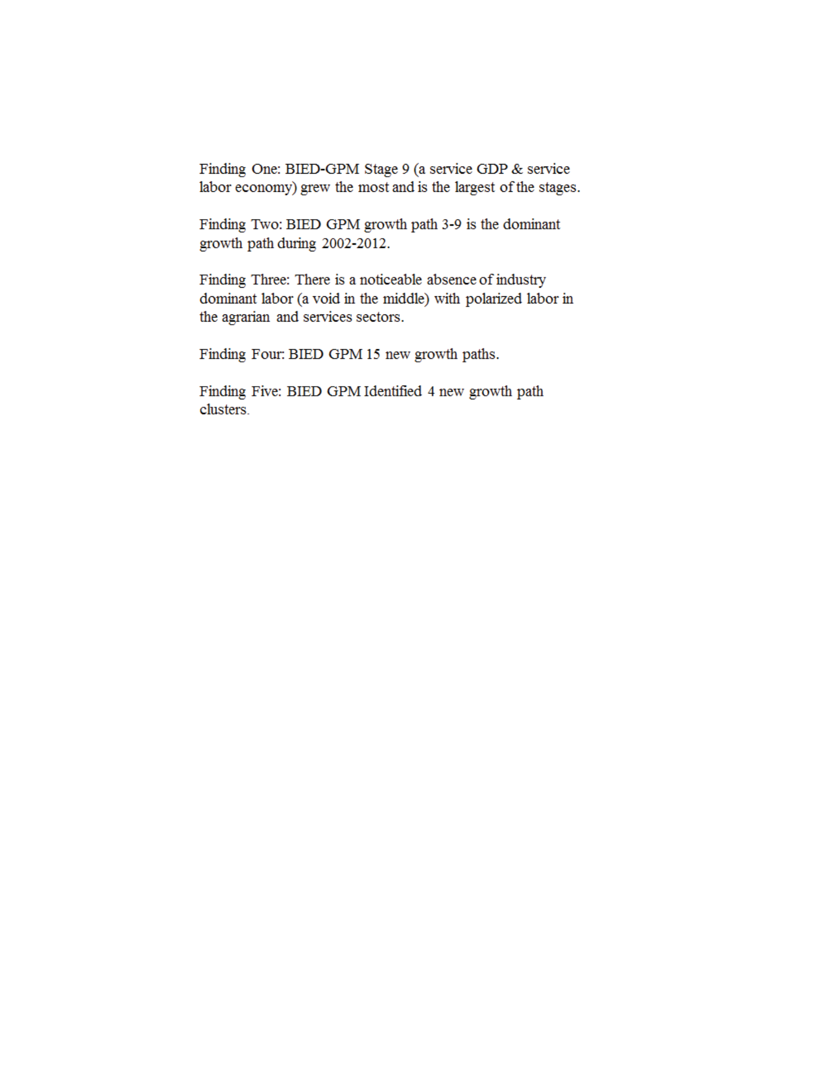
115
Figure 38: BIED-GPM Key Findings

116
Chapter 5: Research Data Analysis
Introduction
Using the Grounded Theory Constant Comparison Method was a way to get new
insight into economic development and behavior economics. Each of the three coding
phases in this study produced new insight to the academic body of behavior economics
and development economics. Three new data sets (products) were identified and can be
called BIED-GPM Stages, BIED-GPM Growth Paths, and BIED-GPM Growth Path
Clusters. Combined, however, the process of looking at economic quantitative data
through a grounded theory constant comparative method to observe new qualitative
behavior helps stimulate new perspectives and generate new theory. This new model
seems helpful at organizing information, forming new labels, and observing the behavior
of these new labeled groups.
Interpretation of the findings
The first data set product identified in this study, is the BIED-GPM stage
identification in both 2002 and 2012. The importance of this new data shows a
disproportional number of nations that are acting similarly to post industrialized nations.
Nations that can traditionally be seen as third world or even second world by other
labeling criteria are seen in this model as stage nine in the BIED-GPM (often considered
a post industrialized stage). This is peculiar, in that, the international organization
labeling systems don’t identify such significant behavior similarities.
The second data-set product that was created identifies 15 new growth paths.
Over time, we can use the constant comparative method to collect additional years of

117
information to help further define the economic behavior paths of nation-states. These
new behavior/GDP growth paths can contribute to statistical probabilities over time.
While probabilities were not calculated here, the notion that this new economic behavior
model can provide a new perspective seems clear, it can and does. While 15 paths were
identified in this study, over time, more may be identified. Studying these growth paths
and the behavior of these paths in comparison to other (nation states) could become a
more stable and consistent method of economic analysis as compared to some of the
international organization models used today. With steps in place to be more scientific in
the labeling than many of the international organization models, a solid foundation can be
created to build broader theories and be potentially more accurate or grounded.
Finally, the third data-set product that was created was the four distinct growth
path clusters, which was identified in the theoretical selective coding phase of this
grounded theory study. These four clusters identify new behavior that can and should be
further researched. These groups could provide significant insight on multiple disciplines
and on many topics. When economic data is reviewed in this manner, several questions
arise. What is the most efficient BIED-GPM stage? What happens in a society that races
to imitate developed post industrialized nations behavior, possibly skipping or racing
through the industrialization phase? If the industrialization phase brings significant
money into the system, if the stage is minimized or shortened, how does the amount of
financial resources in the system impact the service sector later? Put another way, if one
stage is more efficient and brings resources into the nation-state system better than other
stages, should public administrators encourage slowing individuals into a less efficient

118
stage in order to promote long term benefits to the nation stage system? These are
important questions that have been difficult to address until now. With a systematic way
of looking at economic data, future comparisons could be possible and beneficial.
Political labels and classifications seem to have limited use in this capacity. A more
scientific labeling system should contribute to better measurement of nation system
comparison and analysis leading to better public administration management at the nation
state level and possibly individual long term economic prosperity, seen as positive social
change.
Limitations of the Study
The limitations of this study lie with the short time frame of available data,
specifically in the Labor Force by Occupation indicators for developing nations. Using
the Constant Comparison Grounded Theory Method, this limitation in historical data will
get better with time as follow on studies add to the body of knowledge. Better analysis
and comparisons may be facilitated when the database gets bigger. New data sets,
besides the CIA World Factbook should be used to see if the results hold up. There is no
reason to believe that the data sets used or created in this research are misleading, but
additional studies using other data sets could strengthen the findings here.
Recommendations
While many questions arose from this research, the first is what economic growth
stage is the most efficient? While this study does not address this question, it seems to be
an interesting next step. The follow on research suggestions would be to identify what
BIED-GPM has the highest and lowest Gross National Savings rate, Budget Surplus or

119
Deficit, Public Debt, GDP Consumption by Household, GDP Consumption by
Government, GDP Investment in Fixed Capital, GDP Investment in Inventories, GDP
Exports of Goods and Services, and GDP imports of Goods and Services. Inputting these
ten new data sets into the BIED-GPM would strengthen the visibility into a 9
classification system and should give more specific details in the economic growth and
behavior at the nation state system level.
The final recommendation is to continue inputting information into the BIED-
GDP in each year, so exact transition time frames can be measured. While some
historical data is not going to be available, the new transitions can and should be studied
yearly, if not more often. This should help build a body of research and a database that
can identify both positive and negative changes as well as nonlinear economic growth
movements.
Implications
Identifying the most common economic growth path and stage helps show a
movement towards imitation. While individuals desire a high paying services job, does
the rapid movement towards a services dominated economy create alternative problems?
If the services sector is dominated by jobs that “move” money around and the industry
sector is dominated with bringing money into the “nation-state” system, then serious
attention needs to be on the impact of skipping or even moving too quickly through the
industry phases. What is good for the individual level may not be what is in the nation-
state levels best interest? Introduced in a different way, the short term benefit from
pursuing policies that focus on individual gain may be served better by focusing on

120
nation-state policies that promote steady long term growth leading to individual growth
as well as nation-state growth? Does the good of the overall system build a better
livelihood for the population and labor force if there is more money in the system before
it goes to a services dominated cycle? And I believe this to be the most neglected
question in economics, what is the cost of this option to that option? What is the most
expensive BIED-GPM stage, or what stage burns the most cash? These are some of the
proposed follow on research recommendations that can help further define behavior
economics and development economics.
Conclusion
The importance of a nine classification economic model does help develop details
that are not possible with only three or four classifications. While the dominance of
international organizations to collect data, put labels on groups, and impact modern
research is easily understandable, should it be accepted by scientific communities? The
bias of these political organizations or at least the possibility of political conflict should
be a concern. While this data was taken from the CIA World Factbook and the same can
be said for it. The conclusion that many databases should be used to triangulate the
concept this research suggests and to validate the international data and diverse collection
techniques. Not just the CIA World Fact Book data should be used in this BIED-GPM.
I encourage other databases to be used, to see if the results will be similar. The
noticeable absence of a labor dominated industry economy is a concern. Service
dominated economies seem to be in favor. Why are there only two nations (see
Appendix C) with an industry labor dominant economy (stage 4, 5, or 6)? It would seem

121
that stage 5 has the most options and be potentially the most efficient stage from a nation
state perspective. Stage 9 on the other hand seems to favor the individual.
This study identifies five findings, (1) BIED-GPM stage 9 grew the most and is
the largest of the growth path, (2) BIED-GPM 3-9 is the dominant growth path, (3) a
Noticeable absence of industry dominant labor, (4) BIED-GPM 15 identified Growth
Paths, and finally (5) the BIED-GPM identified four new growth path clusters. An
additional note is that qualitative sociology studies like the Classic Grounded Theory
(CGT), constant comparison method can provide insight into complex economic issues.
As a unique way to structure and observe quantitative data, the use of qualitative methods
can and should benefit academic discourse on complex economic activities. Finally, this
study did generate new theory. Economics cannot be properly studied without the
equally important question of cost. With this new labeling system, more precise analysis
and comparisons can be made at the nation-state level. I recommend follow on studies
that help identify the most costly economic stage and the most efficient. Individuals are
going to flock to what they see as the best economic decisions for them and their
families. The social change from this study is this; public administrators need to be the
ones looking out for the best nation state system. If that means slowing down the rate at
which individuals flow towards the service sector from the agriculture sector, than
policies should be used to promote nation state health.
The analogy I like to use when describing this phenomenon is that of a secretary
making $30,000 who buys a $750,000 house. On the surface it looks like the secretary is
successful, as evidenced by a beautiful home. However, after further analysis, we learn

122
that the secretary has committed all the funds available to the purchase and monthly
mortgage payments on the house, but now has no money to fix the roof, mow the yard,
etc. If racing to a service dominated economy with a service dominated labor force was
the answer, more nations would be prospering. Perhaps it is because too many nations
have bought the expensive house before they have an adequate income to properly afford
it. If a stage 9-9 (a service GDP/service labor force) is the most expensive government to
run, than it may help to stay in the industry sector for as long as possible to fill the nation
state system with financial resources. The extra financial capital can help offset other
problems as they arise, making the public administration of the system more stable,
flexible, and adaptable.
New Theory Creation
New theory is the goal from any grounded theory study. The theory created in
this study stems from a formulation of questions brought out by the new insights found in
this research. To start, economics is about efficiency, having efficient markets, efficient
labor forces, and efficient policies. Any economic model should advance the
understanding of markets, labor, or policies. The BIED-GPM does just this. The
Behavioral International Economic Development Growth Path model is nonlinear,
because movement is not always positive, and models should be created to accommodate
negative movement. Behavior economics seems to focus on consumer selection, but that
is only the behavior to part of that economic pie. In order to buy goods or services, first
decisions are made to make money, specifically what sector should be chosen to earn a
living. This study addresses such behavior. This new theory suggests that individual

123
desire for high incomes motivate their behavior to gravitate toward the service sector.
While this seems appropriate from the individual perspective it may not be beneficial
from the perspective of the nation-state. The lack of management and understanding of
this behavior may minimize the importance of this difference at the public policy
decision making level. What is best for the individual may not be the best for the nation-
state. If moving through important industrialization and manufacturing stages bring vital
resources “into” the nation-state system, it can easily be perceived that abbreviating such
an important phase would likely impact the system. What is the most efficient labor
force balance? While this research indicates that most nations are “imitating” the
behavior of post industrialized nations as found in the number of nations in BIED-GPM
stage 9 (Service GDP/Service Labor), more research is needed to address the proper
balance to what is the most efficient use of time in each BIED-GPM stage. Both short
and long term effects should also be studied on the phenomenon of nation-states racing to
BIED-GPM stage 9. This theory could be abbreviated: Nation-state and individual
economic interests diverge through the development process. Finding an efficient
balance between the interests of nation-states and individuals as they move through
BIED-GPM stages can build a stronger understanding of the efficiencies and impacts to
both. Using BIED-GPM Growth Paths and BIED-GPM Growth Path Clusters to help
compare and contrast economic behavior can help promote better policy and
understanding. The BIED theory is that new labels (BIED-GPM Stages) help establish a
sound scientific labeling of nation-states to anchor comparisons of BIED-GPM Growth
Paths in order to improve analysis and comparison in regard to efficiencies. BIED-GPM

124
Clusters add even more qualitative depth to the understanding of behavior in job
selection. The goal of the BIED theory is to find and explain the efficient path through
development at different levels, in this research, the individual economic systems and the
nation-state systems. The BIED-GPM, BIED-GPM Stages, BIED-GPM Growth Paths,
BIED-GPM Clusters are all tools to help compare and analysis data in order to find
efficiencies in the balance between different economic systems.
More research needs to be done to validate this theory, as this research only
suggests such possibilities. Further studies should include costs of government in
different stages, costs of business in different stages, and identification to which stage is
the most efficient, which stage is least efficient, and when enough data has been
collected, what time line is typical with the transition of different stages, and at different
levels of economic systems as well. This study was only ten years and a review of a
longer time frame should contribute to more understanding of these BIED-GPM stages,
growth paths, and clusters.
Social Change
The social change in this study comes with looking at economic information
differently and having a new tool that can help label nation states better, so more accurate
analysis may be possible. Better decision making comes with new perspective and new
tools like the BIED-GPM stages, paths, and clusters. New theory indicates that
individual decisions and nation state decisions do not benefit the nation state the same.
Political borders are important in regard to rules and laws, but political labels can distort
economic activity and labeling. Moving to more accurate labels can significantly

125
improve analysis as individuals and nation-states find balance. Measurements between
more accurate labels may also be possible, contributing to the betterment of social
structures and comprehension. The implications for positive social change from this
research include (1) a new BIED-GPM tool to aid in economic analysis of development
economics and growth economics, (2) new economic labels based more on scientific
principles and less on political or lending preferences, (3) further development of a young
behavior economic sub field, promoting qualitative perspective in a quantitative
dominated field, and finally (4) positive social change is found in augmenting the
perception that individuals and nation-states may not benefit the same from racing to a
service dominant GDP/service dominant labor economy. While individuals desire high
incomes and the lifestyle a BIED-GPM stage 9 (service dominant GDP/service dominant
labor economy) historically provides, nation-states that speed through the industrial stage
may not benefit from having enough financial capital within the system to afford the high
cost of such an economy. More research will help define the impact of this social
change, but this study should help focus attention to the new discipline of behavior
economics and the importance of thinking differently to better the human experience.
A fifth social change element was identified in this research, in the ability of a
sociology research methods contribution to economics. The implications of positive
social change stemming from using an established sociology research method in the field
of economics, specifically in behavior economics and growth economics can help balance
the lop sided quantitative heavy contributions over the last century adding important
qualitative depth improving analysis and understanding in a positive way. This was not

126
the intended purpose of this study, but the contributions of this research method seem to
clearly indicate that positive social change is found by the research method known as
classical grounded theory or grounded theory.

