ECN 360-Introduction causal effects among economic

Introduction causal effects among economic

Empirical and theoretical studies on the causal effects among economic growth, financial

development, and inequality have increased over the last few decades. This is not surprising, as

economic growth is accompanied by financial development. Although financial development has

a favorable function of promoting economic growth, it can bring a dysfunction of increasing

income inequality. In other words, development in the financial sector affects investment in

human capital and/or physical capital; thus, by influencing capital allocation, financial

development can change the aggregate output (which is analogous to economic growth) and the

unemployment rate, with potential implications on poverty and income distribution.

The literature indicates a positive relationship between financial development and

economic growth, but the relationship between financial development and inequality remains

unclear, both theoretically and empirically. For example, the theoretical framework suggested by

Greenwood and Jovanovic (1990) used a theoretical endogenous growth model and provided an

inverted U-shaped hypothesis between financial development and inequality while Galor and

Zeira (1993) provided a linear hypothesis.

The empirical evidence is also controversial. Liang (2006) found that financial

development tends to alleviate unequal income distribution of the urban-rural divide in China.

According to Xie and Zhou (2014), however, income inequality, measured by the Gini

coefficient, steadily increased from 0.30 to 0.55 from 1980 to 2012 despite improved financial

markets in China. In addition, the Gini coefficient for Shanghai, a major city in China and the 8th

largest city in the world, increased from 0.244 to 0.389. The Gini coefficient for Chongqing, a

major city in southwest China and one of five national central cities in China, increased from

0.40 to 0.48, which is much higher than 0.311, the average Gini coefficient for OECD countries.

Just as Chinese economic reform is in the spotlight due to its impact on economic growth,

China’s continuous reforms have affected the depth of its financial sector’s development and

innovation since the late 1970s. As a first step to reform, the Chinese government abolished a

central banking system and set up a two-tiered banking system. When the People’s Bank of

China was designated as the Chinese central bank in the mid-1980s, several types of financial

institutions formed, such as policy banks, equitized banks, city commercial banks, rural

commercial banks, joint-stock commercial banks, and foreign banks2. The Chinese financial

system depends on its banking system, even though stock markets in China have developed

quickly since the 1990s and total market capitalization in the Chinese stock exchange ranks

fourth in the world; and China has the second largest stock market in Asia. On the other hand, in

terms of the financial sector’s size, banks in China are larger than the stock market. Table 1.1

shows that, after economic reform, financial sectors in China have developed rapidly: the ratio of

the money supply (M2) to real gross domestic product (GDP) surged from 0.99 in 1995 to 1.91

in 2014, the ratio of total deposits to real GDP increased from 0.88 in 1995 to 1.77 in 2014, and

the ratio of total loans to real GDP increased from 0.82 in 1995 to 1.27 in 2014. Interestingly,

China, the world’s fastest growing economy, achieved phenomenal growth, became the engine of

global economic growth through stepwise economic reforms and financial development, and

reduced the number of people living below the poverty line. Recently, however, against all

expectations, the Gini coefficient of each province in China sharply increased, which is an

unpleasant scenario for economic growth, financial development, and income inequality.

Table 1.1: Recent Trend of Financial Development in China: 1995 - 2014

M2/ GDP Deposits / GDP Loans / GDP

1995 0.99 0.88 0.82

1996 1.05 0.96 0.85

1997 1.14 1.03 0.94

1998 1.22 1.12 1.02

1999 1.32 1.20 1.04

2000 1.34 1.23 0.99

2001 1.42 1.30 1.01

2002 1.51 1.40 1.08

2003 1.61 1.51 1.16

2004 1.57 1.49 1.10

2005 1.59 1.53 1.04

2006 1.57 1.53 1.03

2007 1.49 1.44 0.97

2008 1.49 1.46 0.95

2009 1.75 1.71 1.14

2010 1.76 1.74 1.16

2011 1.74 1.65 1.12

2012 1.80 1.70 1.17

2013 1.86 1.75 1.21

2014 1.91 1.77 1.27

Source: Chinese Statistical Yearbooks

Early literature focused on the association between economic growth and inequality (i.e.,

Chen, 1996; Kuznets, 1955; Lardy, 1978, 1980; Lyons, 1992; Oi, 1993; Oshima, 1992; Sloan,

1994; Williamson, 1965; Yang, 1996) and on the relationship between financial development and

economic growth. As world financial markets continue to grow rapidly, there is greater

importance on the impacts of financial development. Thus, topics extended to the relationship

between financial development and economic growth (Boyreau-Debray, 2003; Zhang et al.,

2012). In addition, issues on economic growth, financial development, and inequality continue to

focus on the relationship between financial development and inequality (i.e., Atkinson &

Brandolini, 2001; Banerjee & Newman, 1993; Beck, Demirgüç-Kunt, & Levine, 2004; Clarke,

Xu, & Zou, 2003; Galor & Zeira, 1993; Greenwood & Jovanovic, 1990; Liang, 2006; Li, Squire,

& Zou, 1998; Qi , Ran, Mingxing, & Chen, 2003; Tsui, 1993; Wei & Wang, 1997; Wei & Wu,

2001).

With increasing interest in income inequality, Atkinson and Brandolini (2001) questioned

potential problems from the use of a secondary dataset. A potential problem in using secondary

datasets is inconsistency in the definition. Another possible problem in using Gini coefficients

for cross-country analysis is the use of different source data. For example, when we calculate a

Gini coefficient, the primary source of data is from a national household survey. However, other

administrative data can be used as well, so the data source for calculating a Gini coefficient can

differ.

In this paper, I describe various literature on economic growth, financial development,

and inequality, including theoretical and empirical studies, using a cross-country analysis and a

Chinese sample. The paper is organized as follows. Section 2 reviews the relationship between

economic growth and income inequality in China, including a theoretical framework and

empirical evidence. Section 3 describes the relationship between financial development and

economic growth in China. Lastly, Section 4 reviews a theoretical framework and empirical

evidence on financial development and inequality in China.

1.2 Economic Growth and Inequality

The theoretical studies, empirical works, and political worries about the course of income

inequality as the product of economic growth have brought the causal link between economic

growth and income inequality to the forefront. In the following, I review literature on economic

growth and inequalities and then describe empirical evidence using a cross-country analysis and

a Chinese case.

1.2.1 Early Theoretical Framework on Economic Growth and Income

Inequality

Much theoretical and empirical research on economic growth and income inequality has

its roots in the classical contributions of Kuznets (1955). He created a theoretical framework to

hypothesize that economic growth is linked to inequality in an inverted U-shaped pattern, where

income inequality widens at the first stage of development and then is reduced at the later stage

of development. In the early stages of an industrial revolution, a country experiences

urbanization, where cities are the center of the country’s economy. As former workers in a rural

area migrate to the city for high paying jobs in an industrialized urban area, the income

disparities between urban and rural areas increase. When income per capita approaches a certain

point, income disparities between urban and rural areas are expected to be lower due to the

emergence of a new industrial system, such as free market economy, which facilitates additional

rapid economic growth. Therefore, Kuznets suggested that the level of income inequality can be

explained by an inverted U-shaped curve since the level of income inequality increases in the

early phases of economic growth, like low-income countries or developing countries, and after

achieving a certain point, the level of income inequality decreases again in later phases of

economic growth, like high-income countries or developed countries. In a simple model,

Vijverberg (1991) examined the contributing factors to inequality in a growing economy. Using

the model, the author attempted to analyze the phenomenon: why some countries experienced a

higher income inequality during the growth process while other countries mingled fast economic

growth with a good record of income distribution? Under a monotonic saving rule (i.e., a family

that owns more capital saves at least as much as a family that owns less capital), the conflict

between equity and growth (i.e., higher inequality and higher growth) is not due to “wealthy

families save more”. Rather, the conflict is caused by the condition that the inequality of saving

is strictly greater than the inequality of capital ownership. The conditions for an economy to be

in conflict and/or non-conflict regimes were analyzed in details. Under a non-monotonic saving

rule, Vijverberg (1996) incorporated social class mobility and macroeconomic conditions in the

conflict/non-conflict analysis of equity and growth.

Barrios and Strobl (2009) suggested a theoretical model to analyze the dynamics of

regional growth. Once a technological innovation takes place in a specific region, this region

would receive the benefits of a high rate of growth at the initial stage of economic growth. The

other regions will catch up to this leading region with a lag, and the length of this lag depends on

differing technological capabilities. Thus, regional inequalities increase at the first stage of

technological innovation and later decrease after achieving the peak of regional inequalities. This

is because lagging regions adopting technological innovation will develop at the same rate with

those of the leading region and then will have additional growth impact from the natural rate of

convergence. This model suggests an inverted U-shaped hypothesis in the short run, while

Kuznets’ hypothesis focuses on long-run structural changes. Turnovsky (2015) developed a

model to investigate the association between economic growth and income inequality focusing

on public investment as a key determinant of the association. He suggested a general equilibrium

growth model with heterogeneous agents, which is characterized by homogeneity of the utility

function and the same unrestricted access to perfect factor markets for all agents. In this model,

government investment promotes the productivity of private capital, encouraging its

accumulation. Thus, under the unequal distribution of private capital among agents, government

investment increases wealth inequality over time.

1.2.2 Empirical Evidence on Economic Growth and Income Inequality

First, I describe literature on the relationship between income inequality and economic

growth for developed or developing countries using a cross-country analysis. Next, I describe the

relationship between economic growth and income inequality in China.

Williamson (1965) depicted patterns of regional inequalities under the process of national

development using examples of the U.S., France, Italy, Spain, Germany, Canada, Brazil, Sweden,

Australia, Norway, and India by focusing on a new popular phenomenon of regional income

inequality known as the North and South Problem, which illustrates the absolute differential

between rich and poor areas. The cross-country analysis found that economic development and

regional inequality have the following pattern. As the national economy grows and expands, the

degree of regional inequality narrows. Among the countries in the sample, Spain, Italy,

Columbia, and Brazil, nations below the middle-income class, did not generate the expected

conclusion that lower income per capita is associated with greater income inequality. U.S. data,

however, generated what was expected − the lower income per capita, the greater income

inequality. In addition, data on Germany, Sweden, France, and Canada showed that regional

inequality widened substantially at an early stage of economic development, while regional

inequality was reduced as the national economy matured. In conclusion, the gap between the rich

and the poor is deeper in the agricultural sector than in the industrial sector.

In another influential study, Ahluwalia (1976) studied the relationship between economic

growth and income inequality using a cross sectional data set of 14 developed countries, 40

developing countries, and six socialist countries, creating a multivariate regression model to

examine the cross-country association between development process and income inequality. The

empirical results strongly support the hypothesis that income inequality widens at the beginning

of economic development and then decreases in the later stages of economic development.

Secondly, the average real income of the lower percentile group increased as the gross national

product (GNP) per capita increased, even though the speed of increasing real income for the

lower percentile groups was more gradual than for the upper income groups. Finally, the findings

do not support the view that higher income inequality is related to faster economic growth.

Oshima (1992) discussed Asian income distribution trends in relation to the inverted Ushaped

curve. The Asian income distribution trends corresponded to the inverted U curve; however, the

peak of the Asian income distribution trends differed from Western countries except for Japan,

whose income inequality trends are similar to the trends of Western countries. More specifically,

the peak of Asian income inequality trends was achieved earlier in the course of development

growth than those in Western countries. While the Gini coefficient of Western countries

decreased in the 1920s when income per capita exceeded $2,000, the peak Gini coefficient of

Asian countries was reached when income per capita exceeded $1,000. This is because Asian

countries are aligned to the agricultural sector, while Western countries are aligned to the

industrial sector.

Although there is no strong supportive evidence that economic growth influences income

inequality, Psacharopoulos et al. (1995) looked at how a period of recession during the 1980s

affected income inequality of 18 Latin American countries. Unlike Kuznets’ (1955) inverted

Ushaped curve for a long-run relationship, the authors investigated short-run cyclical behavior

between growth and inequality based on micro data obtained from household surveys. The

reduction in economic growth widened income inequality among the Latin American countries

and an increase in economic growth decreased income inequality measured by the Gini

coefficient and the share of wealth of the bottom 20th percentile. Since economic crisis exerts

downward pressure on wages and employment, employees were forced to agree to wage

deductions or become unemployed and, therefore, income inequality deteriorated.

In another cross-country analysis on economic growth and income distribution, Ravallion

and Chen (1997) researched the empirical link between economic growth and income inequality

using a data set of 67 developing countries from 1981 to 1994. To provide alternative measures

of distribution and poverty, the authors analyzed the relationship of poverty changes with

economic growth. They found that higher growth rates tended to reduce the rates of poverty over

the between 1981 and 1994. Overall, for the whole sample, the increase in average consumption

was connected to reduced income inequality. However, when data from Central Asia and Eastern

Europe were excluded, income inequality tended to widen. This empirical finding is not robust

since the negative coefficients of the economic growth measures were insignificant. In addition,

the authors found that income inequality was not associated with average consumption growth

when dropping the countries of Eastern Europe and Central Asia. They found that growth in

average living standards was strongly associated with the rates of absolute poverty reduction.

Scully (2002) researched the association between economic growth and inequality using a

cross-country dataset of developed and developing countries in Asia for 1975, 1980, 1985, and

1990. A main finding is that in a regression equation that explain the Gini coefficient (a measure

of income inequality), the slope of the degree of economic freedom is negatively significant,

suggesting that more economic freedom, a measure of the role of government policy in

stimulating economic development and in reducing income inequality, is associated with a

decrease in income inequality. Also, the estimate of the effect of economic growth on inequality

was negative and statistically significant, which means income distribution equalized as the

economy grew and expanded. In conclusion, a higher degree of economic freedom resulted in

more equal income distribution, and economic growth improved income disparity.

However, Atkinson and Brandolini (2001) and Clarke et al. (2003) exposed potential problems in

the comparative analysis using cross-country data, stating that secondary crosscountry data has

problematic issues related to data quality and data consistency. These potential problems will be

discussed later in detail. Instead of using a cross-sectional dataset, Krongkaew and Kakwani

(2003) analyzed how economic growth affects income inequality in Thailand, one of the fastest

developing countries in Asia, using a dataset between 1962 and 2000. They found that the

number of people under the poverty line decreased as GDP increased due to the increase on the

growth rate of GDP, but Thai people’s income distribution became less equal. According to these

findings, the association between economic growth and income inequality conforms to the

Kuznets curve, which indicates an increase in inequality as starting from a lower level of

development. In addition, the authors found that the impact of economic growth on poverty

reduction is offset by a high degree of unequal income distribution.

Recently, Fawaz et al. (2014) examined the effect of income disparities on economic

growth applying system GMM based on World Bank classifications (56 countries classified as

high-income developing countries and 55 countries classified as low-income developing

countries) from 1960 to 2010. Their findings revealed that income inequality is positively

associated with economic growth measured by per capita GNP in high-income developing

countries, while income inequality is negatively related to inequality in low-income developing

countries.

1.2.3 Economic Growth and Income Inequality in China

Next, I turn to research related specifically to economic growth and income inequality in

China. Lardy (1978) examined how the Chinese government regulated resource allocation, the

relationship between these government policies and the pattern of economic growth, and the

association between these policies and income distribution in China. The paper described the

adoption of the Soviet model of planning, which is about the extension of central control to

functional areas in the Chinese economy. This intensively centralized system was quite

successful in inducing investment and accelerating economic growth in China. However, these

radical policies for a vertical relationship between economic planning and management severed

developmental relations among local governments that had no economic cooperation in their

provinces. A centralized system on decisions resulted in inefficiency as well. In addition,

although a causal relationship between economic growth and the rise of income inequality was

not completely discovered, the paper found that planned economic control can mitigate the

negative distributive outcomes of economic growth.

1.2.3.A Economic Growth and Income Inequality at the Urban-Rural Level

The central government set in motion many transitional measures that positively

influenced the economic welfare of Chinese rural areas (Oi, 1993). While people in rural areas

improved their income, the income gap between urban and rural was extraordinarily high in

China compared to other developing countries in Asia between 1978 and 1990. According to the

paper, the main source of income inequality in China came from the gap between the urban and

rural income during this time. Examples of the central government’s policies are the following:

revising urban-biased pricing for grain under the procurement plan and relaxing of the rural

economy structure permitting people in rural areas to diversify to more profitable grain and to

involve the industrial sector rather than the agricultural sector. These reforms were not

considered persistent shifts to a rural bias reform, and economic development of rural areas in

China was not the fruit of urban or rural bias but the result of local governments’ efforts. Yang

and Wei (1996) summarized several key factors that led governors to rethink regional

inequalities and key policies, such as credit availability, tax incentives, and interregional

cooperation, to decrease income disparities. The income gap between rural and urban areas in

China doubled between 1965 and 1992. Since the State Council decided to stimulate rural

enterprise development in order to reduce rural-urban income gaps, several forms of government

policy remarkably preceded rural enterprises’ development. Many local governments and

enterprises accepted and instantly applied the central government’s policies, which favored rural

enterprises’ interests. However, the central government’s effort to decrease regional inequality

did not properly reduce the gap between the coast region and the inland area. Chinese leadership

recognized the economic gap between urban and rural areas. As a result of their recognition of

the urban and rural gap, a session of the National People’s Congress in 1995 emphasized

economic development policies of inland regions and ethnic areas, such as intergovernmental

fiscal transfers and foreign investment.

1.2.3.B Economic Growth and Income Inequality at the Province Level

Unlike previous research on economic growth and income inequality at the urban and

rural level, Lyons (1992) re-examined the Chinese model of development in terms of provincial

growth and income inequality at the province level. New provincial income data released by the

State Statistical Bureau in China from 1952 to 1987 and the coefficient of variation, a measure of

income inequality, were utilized for the analysis of economic growth and income inequality. The

author summarized the dispersions of each measure, net material product as an output measure

and the coefficient of variation as a measure of inequality, to look into within provincial level

disparities. First, the analysis on output data captured provincial disparities at the initial stage of

development. Based on the analysis of dispersion, overall growth rates and industrialization rates

are quite different among provinces, and the evidence related to consumption shows a solid trend

toward narrowing inequality across the Chinese provinces in terms of relative distribution.

Disparities in growth rates in consumption are similarly compressed by transfers among

provinces and by separating consumption from output in non-agriculture. In sum, the author

argued that interprovincial inequality has narrowed since 1983.

Chen and Fleisher (1996) examined the relationship between regional inequality and

Chinese economic growth by focusing on the impact of the growth process during the post-Mao

transformation period on provincial inequality. Based on panel data between 1978, which was the

beginning of the economic reform, and 1993, they saw that overall provincial inequality

measured by the coefficient of variation narrows but that the inequality between coastal and

noncoastal regions increases somewhat. This is mainly because government encouragement and

private investment incentives create a significant income gap among provinces in China.

1.3 Financial Development and Economic Growth

1.3.1 Characteristics of Financial Development in China

A developed financial system facilitates transactions, mobilizes savings, allocates these

funds to economic activities, and supervises the activities of the recipients of those funds. A well-

developed financial system accompanying these roles enhances economic growth (Levine,

1997). On the other hand, an underdeveloped financial system leads to as misallocated credit,

misplaced loans, and poorly managed borrowers, which may harm economic growth (Calomiris

& Hubbard, 1990). China’s economy has grown tremendously since its initial economic

transition in 1978. China has now become part of the Group of Two (G2) along with the United

States as the two most influential and powerful countries. According to Allen et al. (2005), there

is a high probability that China will be the world’s largest economy within 10 years based on

purchasing power parity (PPP). As is well known, China’s tremendous growth has been

accompanied by its financial development. That being so, Allen et al. (2005) argued that China is

a counterexample to the conventional relationship between finance and economic growth.

China’s banking system transition was initiated in the early 1980s. The four state owned

specialized banks, called as The Big Four, started to accept deposits and engaged in banking

activities in the 1980s. Even as the Big Four converted to publicly-listed banks and as more

domestic/foreign banks joined the system, the Chinese government still has a dominant impact

on banks’ activities. While China has experienced a huge transformation in the financial sector,

four major state-owned banks possess over 60% of the total financial assets in China. However,

the banking sector’s efficiency is poor since it is dominated by four large state-owned banks.

The state-owned banks were inefficient. In 1978, China separated the People’s Bank of

China from the Ministry of Finance. Then in 1979, the Chinese government re-founded the Bank

of China, the People’s Construction Bank of China, and the Agricultural Bank of China so they

might compete for lending services and savers. In 1983, the People’s Bank of China was

designated as the central bank. In addition, the Industrial and Commercial Bank was founded to

provide more financial services. It is now the largest bank in China with half of all bank lending.

Additionally, three smaller national banks (Everbright, Hua Xia, and Min Sheng) entered the

Chinese banking sector and a number of regional banks opened in 1987 and 1988. Different

types of non-bank financial service providers, such as trust and investment firms: urban credit

cooperatives: and financial service companies that provided securities, credit rating, and financial

leasing services, were established in the mid-1980s. The Chinese government generated a variety

of structural changes in the financial system, but policy loans are the prominent characteristic of

its financial structure. In fact, by the end of 1991, policy loans made up 67% of Bank of China’s

assets, 51.2% of Agricultural Bank’s assets, 58% of the Construction Bank’s asset, and 25% of

Industrial and Commercial Bank’s assets (Cull & Xu, 2000). Lastly, an important point of

Chinese financial structures is that 25% of state owned enterprises’ (SOE) loans depended on

direct government transfers in the early 1980s. This decreased to about 2% between 1990 and

1994. In contrast, the proportion of bank finance not dependent on government transfers

increased from 15% to 32% between 1980 and 1987.

Cull and Xu (2003) analyzed the link between bank finance and state-owned enterprises’

productivity in China from 1980 to 1994. Using a probit model where the dependent variable is

access to finance and a tobit model where the dependent variable is the share of total finance,

Cull and Xu (2003) found that bank finance is positively correlated with SOEs’ profitability. Its

positive association between bank finance and profitability was stronger in the 1980s. However,

in the 1990s, the positive association between bank finance and SOEs’ profitability weakened

since the responsibility for SOE bailout moved from the government to banks. Additionally, the

authors did not find any strong association between direct government transfers and SOEs’

profitability in the 1980s and 1990s.

A second stage of financial reforms in China occurred between 1994 and 2000. Initially,

three policy banks for policy lending were founded in 1994 and the central bank adopted indirect

monetary control. Later, in 1995 the central bank enacted the Commercial Bank of Law of China

to establish pivotal elements for the operation of commercial banks. In 1998, the Chinese

government ceased credit planning for state-owned commercial banks. Lastly, in the late 1990s

the Chinese government restructured state-owned commercial banks and founded four Asset

Management Companies using 270 billion Yuan of government money. Notably, in 1996 the first

private-owned bank, China Minsheng Bank Corporation, was founded and 13 national

jointequity commercial banks were established by the beginning of 2000.

Since China’s entrance into the World Trade Organization (WTO) on December, 2001,

China has taken more active policies such as liberalization of the interest rate, relaxation of

regulations on foreign banks, and mitigation of restrictions on ownership takeovers to encourage

non-state financial intermediaries along with more foreign banks entering into domestic credit

markets. After WTO entry, the Chinese government established the China Banking Regulatory

Commission (CBRC) in 2003 to improve asset quality, risk control, and capital adequacy.

Consequently, since the CBRC forced all newly founded shareholding commercial banks to have

one or more foreign strategic investors, restrictions on foreign investors and banks have relaxed

and the number of foreign banks has sharply increased. At the end of 2006, there were 223

foreign banks from 42 countries and 242 representative offices (Wang & Zhang, 2009).

1.3.2 Theoretical Framework on Financial Development and Economic

Growth

This section reviews theoretical works on the association between financial development

and economic growth. The cost of obtaining information or enforcing financial contracts brings

the need for financial intermediary development. According to Merton and Bodie (1995), the

efficiency of financial intermediaries affects the redistribution of financial resources. When

banking sectors’ efficiency improves, the cost related to obtaining information and transactions is

reduced and credit allocation is more efficient. Similarly, as stock and bond markets mature,

people gain more investment opportunities that, in turn, make this investment more liquid than

conventional savings. In brief, market frictions due to imperfect credit markets motivate financial

intermediary development and, again, these more advanced financial markets improve efficiency

that can affect economic growth. According to Levine (2005), a well-developed financial system

enables reduction in the cost to produce information, monitor investment activities, manage risk,

and to mobilize.

Boyd and Prescott (1986) argued that financial intermediary development reduces the

cost for producing information and allocating capital in ways that may improve the allocation of

financial resources since people are confronted with the high transaction cost connected with

examining firms’ and managers’ financial soundness. Therefore, the emergence of financial

intermediaries that extend loans and accept savings reduce the cost of producing information on

possible investment. Greenwood and Jovanovic (1990) suggested a model for the dynamic

relationship between finance and economic growth. Like Boyd and Prescott (1986), they agree

that financial intermediary development generates preferable information with the least

transaction cost, improves the allocation of financial resources, and, therefore, promotes

economic growth. However, unlike Boyd and Prescott (1986), Greenwood and Jovanovic (1990)

pointed out that when each investor utilizes financial intermediaries to reduce the cost related to

examining the soundness of firms and managers and to investigating economic situations, it is

still costly. In their argument, credit accessibility, which is mostly provided by financial

intermediaries, is necessary for the implementation of investment activities and business projects.

For this reason, as more investors are able to utilize financial services offered by financial

intermediaries, the ability of financial intermediaries to produce information on possible

investments and to allocate capital will be improved.

Lastly, Galor and Zeira (1993) discussed a linear relationship, which implies that a

welldeveloped financial system reduces income inequality. Imperfect financial markets harm

economic growth because misallocated credit prevents individuals from investing into human

capital. Since the accumulation of human capital is negatively affected by capital market

imperfection, the initial wealth distribution has an impact on who has a chance to utilize the

credit resources in order to accumulate human capital.

Stiglitz and Weiss (1983) argued that if monitoring investment does not work properly

due to an underdeveloped financial system, this imperfect system may impede the mobilization

of capital resources from possible investors and savers. Thus, monitoring investment activities

derived from a well-developed financial system affects firms’ performance accompanied by large

capital investment and, in turn, influences economic growth.

Efficient capital mobilization is necessary for economic growth. As discussed already,

one barrier to mobilize financial resource is the fixed cost of transaction and information

acquisition on possible investments, which can be alleviated by the efficiency of financial

intermediaries. Sirri and Tufano (1995) argued that these imperfect market frictions, which cause

high transaction and information acquisition costs, can be alleviated by financial intermediaries

who provide reliable financial products to investors and savers. Therefore, financial

development, which fosters mobilizing financial resources, can stimulate economic growth by

boosting capital investment. In another influential study by Acemoglu and Zilibotti (1997), one

of main advantages of mobilizing financial resources is to create a small denomination

investment, which allows individuals to diversify risks, and attract more investment and savings

from small investors or savers. As a result, financial development supports the reallocation of

existing financial resources and, therefore, gives positive spillover on economic growth. Aghion

et al. (2004) suggested a model to analyze how the ability of companies to access credit affects

technological innovation and growth in the long run during recessions. Assuming there exists

adjustment costs to research and development (R&D), the model incorporates whether

companies invest into low return investments or into R&D, which can enhance companies’

growth but might be more risky. Thus, a well-developed financial system enables firms to

decrease adjustment costs to R&D, which promotes the ability of firms to access credit for

technological innovation, while under-developed financial systems reduces firms’ accessibility to

credit due to relatively high adjustment costs to R&D.

Recently, Laeven et al. (2011) suggested a theoretical model reflecting the profit

maximization behaviors to explain how financial innovation has been a driving force of financial

development and economic growth. In their model, lenders try to screen potential borrowers,

companies, and to innovate better ways to screen borrowers. Financial innovation, which creates

more effective screening, improves the rate of technological innovation, which affects economic

growth. Again, this technological innovation positively affects financial innovation, which is

endogenous coevolution of financial and technological innovation.

1.3.3 Empirical Evidence on Financial Development and Economic Growth

The impact of financial intermediary development on economic growth is frequently

debated and convincing empirical evidence indicates that financial intermediary development

accelerates economic growth. In assessing the impact of financial development on economic

growth, some researchers used a pooled cross-country dataset, including developed and

developing countries. Joseph Schumpeter (1911) showed that financial services, such as

mobilizing savings, evaluating projects, facilitating transactions, monitoring managers, and

managing risk, are necessary for economic growth. King and Levine (1993b) investigate

Schumpeter’s view with a dataset of 80 countries between 1960 and 1989. To measure the degree

of financial development, they suggested a ratio of liquid liabilities to GDP, the importance of

deposit banks relative to the central bank, the ratio of credit issued to non-financial private firms

to total credit, and the ratio of credit issued to nonfinancial private firms to GDP. Their results

indicate that a higher degree of financial development is related to greater economic growth,

physical capital accumulation, and improvements in economic efficiency. Furthermore, a higher

degree of financial development is connected to efficiency improvements and accelerating

capital accumulation in the long run.

By means of a cross-country dataset of 63 countries from 1960 to 1995 and dynamic

panel techniques, Beck (2000) examined the empirical relationship between financial

development and real per capita GDP growth, total factor productivity growth, the accumulation

of physical capital, and the rates of private savings. But Beck (2000) found that a higher degree

of financial development brings about greater economic growth. While previous literature

focused on the relationship between financial development and economic growth, Beck also

focused on the relation between financial development and the sources of economic growth, such

as private savings rates, physical capital accumulation, and total factor productivity. Financial

development was positively associated with economic growth and total factor productivity

growth and these rigid links do not arise from unobserved country specific effects or

endogeneity. However, the relationship between financial development and both physical capital

growth and savings are not clear.

In another study, Rioja and Valev (2004) tested whether financial intermediary

development affects capital accumulation and productivity using a cross-country dataset of 74

countries and GMM dynamic panel techniques. Three financial development measures were

constructed: the ratio of the credit issued to the private sector to the GDP, the ratio of commercial

bank assets to commercial plus central bank assets, and the ratio of currency plus demand and

interest-bearing liabilities of banks and non-bank financial intermediaries to GDP. Findings

revealed that financial development was significantly and positively associated with economic

growth, productivity growth, and capital growth. Subsequently, a cross-country dataset of 74

countries was classified into low-, middle-, and high-income countries. For middle and high-

income countries, the estimated coefficients of each financial development measure were

positive and statistically significant at the 1% level. For low-income countries, however, the

estimated coefficients of each financial development measure were not statistically significant.

More interestingly, in terms of the coefficient’s magnitude, high-income countries’ estimated

coefficient was larger than that of middle-income countries’ estimated coefficient. This implies

that the impact of financial development on economic growth varies considerably depending on

capital accumulation.

Next, I review literature on whether financial intermediary development affects economic

growth in China. The majority of evidence concludes that financial development causes higher

economic growth. Boyreau-Debray (2003) explored the province level relationship between

financial intermediation and economic growth in China by applying the traditional growth

regression framework to a panel of provinces in China. First, arguing the fragmentation of

regional capital markets, the author justifies the existence of local credit channels. Next, with 26

Chinese provinces over the period of 1990 and 1999, the author analyzed the impact of financial

sector development on economic growth using the GMM system estimator. Credit extended by

the financial sector at the province level had a statistically insignificant negative effect on a

province’s economic growth. In other words, the financial deepening in China did not increase

provincial economic growth despite evidence that financial development in China contributed to

its national economic performance.

Zhang et al. (2012) assessed even greater fragmentation of financial markets at the city

level. Based on a dataset of 286 Chinese cities between 2001 and 2006, Zhang et al. (2012)

analyzed the impact of financial development on economic growth by applying traditional

firstdifferenced and system GMM estimators. The Chinese dataset does not allow calculation of

traditional indicators of financial development such as the ratio of credits extended by financial

intermediaries to private sector to GDP at the city level. Thus, the authors employed the

following indicators to measure financial development: 1) the ratio of total loans to GDP to

measure financial depth; 2) the ratio of total deposits to GDP to capture the size of financial

intermediaries; 3) the ratio of total household savings to GDP to measure the degree of

household saving mobilization; 4) the ratio of fixed asset investment by domestic loans to

investment by state government to capture the substitution of more market and profit oriented

financial transactions for state government to allocate capital more efficiently; and 5) the ratio of

deposits by firm to total deposits in financial system to measure how financial development

contributes to provide banking service to corporations. Their results suggested that financial

development has a positive impact on economic growth. In other words, financial deepening, as

measured by the size and depth of the financial sector, contributed to Chinese economic growth,

and financial development after WTO entry spurred economic growth in China. However, Law

and Singh (2014) found that financial development has a negative impact on economic growth

after a certain threshold level. In other words, the relationship between financial development

and growth is contingent on the level of financial development, where financial development

increases economic growth after a level of financial development surpasses a certain threshold

level. They suggested innovative dynamic panel threshold technique to investigate the

association between finance and economic growth based on 87 developed and developing

countries for the period 1980 to 2010. Their empirical findings indicated that the degree of

financial development has a positive impact on economic growth only up to a certain threshold.

After a certain threshold, further financial development has a negative impact on economic

growth.

1.4 Financial Development and Inequality

1.4.1 Theoretical Framework on Financial Development and Inequality

Greenwood and Jovanovic (1990) introduced a non-linear relationship between financial

development and inequality, which indicates an inverted U-shaped curve – at the early stage of

financial development, due to limited access of credits to poor people, income disparities

increase, and then after a certain stage, financial development decreases income disparities. The

authors set up a model where financial development can enable people to access the information

on risky investment by acquiring and analyzing information so that the development of financial

intermediations can contribute to diversify risk of the investment. Moreover, in their model, the

cost of joining a financial intermediary is fixed, whereas financial intermediaries take advantage

of economies of scale in screening projects. Resource allocation efficiency can be promoted by

joining the financial intermediary to stimulate economic growth. In a sense, economic growth

occurs when more people are able to access financial intermediaries, allowing them access to

higher expected return projects. Under this condition above, financial development affects the

relationship between growth and income distribution. The inverted U-shaped hypothesis tells us

the following. At low levels of economic development where financial development is less

mature in their early developmental stage, fewer people are able to join financial intermediaries

since the fixed costs to join are high. Thus, economic development is slow and income inequality

is quite small. If financial sectors are quite well developed (more developed than at the early

stage) in the middle of the developmental stage, economic growth is faster and income inequality

increases more than the early stage of financial development. Lastly, if financial development is

fully mature at the maturity level, income inequality will decrease again because more people

can enjoy the full range of benefits from a formal financial system and be quite stable at the end.

In summary, based on the inverted U-shaped hypothesis suggested by Greenwood and Jovanovic

(1990), at the early stage of economic development, financial development increases income

inequality. However, as the country reaches a stage where more low-income people have easier

access to credit, income inequality will decrease.

Liang’s (2006) empirical analysis provides strong evidence to the linear hypothesis

(Banerjee & Newman, 1993; Galor & Zeira, 1993). The theoretical model by Galor and Zeira

(1993) studied the relationship between income distribution and macroeconomics by investment

in human capital. Under the assumption that the credit market is imperfect, the wealth

distribution affects aggregate output and investment activities in human capital in the short run.

For this result to be effective in the long run as well, the authors added an element of

nonconvexity to their theoretical model, which refers to indivisibility in investment in human

capital. When credit markets are imperfect and a fixed cost connected with schooling is high,

only rich dynasties are able to invest in their human capital. Thus, an imperfect financial market

system hinders the poor from accumulating human capital.

In the face of a credit market’s imperfections and indivisibilities in investment in human

capital, the wealth distribution in conjunction with financial market imperfection influences

aggregate levels of human capital and aggregate output level. If wealth distribution is not quite

equal, fewer individuals accumulate human capital so that it will decrease aggregate efficiency

and, thus, economic growth. In the existence of financial market imperfections, economic growth

in the long run and the persistence of inequality depend on the initial wealth distribution. The

theoretical model by Galor and Zeira (1993) shows that credit accessibility will increase as a

financial market develops. As more low-income people are able to borrow money to invest in

their human capital, economic growth increases and inequality is reduced.

As a recent theoretical work on financial development and inequality, Bumann and

Lensink (2016) developed a tractable model that portrays the relationship between agents having

different investment abilities and banking sectors. As two possible interventions, which liberalize

the banking sector, this tractable model introduces an increase in the size of foreign investments

and a decrease in reserve requirements, which can be utilized to raise domestic loans. The

efficiency of banking sector and the adjustments of interest rates, which influence agents with

varying investment abilities, can be improved by financial liberalization or financial depth. Their

tractable model suggests that financial liberalization will decrease income disparities when

financial depth is high.

1.4.2 Empirical Evidence on Financial Development and Inequality

As discussed above, theoretical models for the linear and inverted U-shaped hypotheses

have distinct predictions for the link between financial development and income inequality.

Clarke et al. (2003) explored the relationship between financial development and income

inequality using a dataset of 91 countries over the period 1960 to 1995. They found strong

support for an inverse linear association between financial development and income inequality,

which is the linear hypothesis suggested by Banerjee and Newman (1993) and Galor and Zeira

(1993). They did not support the inverted-U shaped hypothesis since the coefficients of the

squared term for the financial development measures were not statistically significant.

Incidentally, their main findings provide some supportive evidence for an augmented Kuznets

hypothesis, where the industrial structure (industrial, agricultural, service sectors) is necessary to

explain the association between economic development and income inequality. The authors’

conclusion was that financial development may decrease income inequality since the coefficients

of financial development indicators were negative and statistically significant.

Wei and Wu (2001) studied the association between urban-rural income inequality and

the degree of openness in trade using 100 Chinese cities over the period from 1988 to 1993. The

authors constructed the urban-rural income ratio to measure income disparity between urban and

rural areas and used a ratio of total export to GDP to measure the degree of openness at the city

level rather than the aggregate of urban and rural due to data limitation. The empirical findings

suggested that Chinese cities having a higher ratio of trade to the GDP tended to reduce the

urban-rural income disparity.

Next, domestic income disparity in China, which differs from a cross-country analysis of

income disparity, is discussed. Tsui (1993) decomposed Chinese regional disparities into five

different categories: within-province level, inter-province level, within rural level, urban and

rural, and within-urban inequality. Based on 2306 counties and cities in 1982, the author used

gross value of industrial and agricultural outputs, infant mortality rate, and illiteracy rate to

capture various aspects of regional disparities. The findings indicate that the inequality of

withinprovince level is dominant sources of regional inequalities.

Liang (2006) tested the two theoretical hypotheses on the link between the financial

development and income inequality based on the system Generalized Method of Moment

(GMM) estimator. Empirical results support the linear hypothesis that the development of the

financial sector decreases urban income inequality. All measures of financial development were

significant with the expected signs. After adding the squared terms of the financial variables into

the model to test the inverted U-shaped hypothesis, the financial measures were not statistically

significant, which does not support the inverted U-shaped hypothesis by Greenwood and

Jovanovic. In conclusion, after the Chinese government launched radical urban reforms, the

development in the financial sector triggered a decrease in income inequality. According to

Liang (2006), financial development significantly reduced income inequality in China.

However, it is still controversial whether financial development helps to decrease income

disparity in China. First of all, many significant reforms and institutional innovations in the

financial sector occurred between 1995 and 2010. The Chinese financial system solidified after

the Chinese government announced the Central Bank Law and the

Commercial Bank Law in 1995. Large money injections occurred in 1998 to relieve the heavy

debt of four major state-owned banks and in 2003 to restructure state-owned banks to joint-stock

commercial banks with stock market public listings. When China joined the WTO, its banking

system was required to be fully open to foreign competitors by 2006. Therefore, we need to

investigate the recent Chinese data covering the late 1990s and early 2000s to the present, which

captures an important moment in Chinese banking sectors’ reform after WTO entry. Li,

Squire, and Zou (1998) found that cross-country variations of inequalities were significantly

larger than within-country variations of inequalities. They used a dataset on Gini coefficients of

2,480 observations covering 112 developed and developing countries from 1947 to 1994. They

also examined the determinants of income inequality, looking at policies that are beneficial to the

rich but may not be favorable to the poor, and imperfections in credit markets. The authors

adjusted the data to achieve a more balanced panel dataset and observed that wellequipped

financial markets reduce income disparity.

Similarly, Beck, Demirgüç-Kunt, and Levine (2004) examine that well-developed

financial sectors decrease poverty. They first tested whether a developed financial system

influences the income of each economy’s poorest 20%. Second, the authors investigate the

association between financial development and changes in income distribution. Lastly, they

introduced direct measures of poverty alleviation (the growth rate of the fraction of the

population living under $1 per day), testing whether the developed financial system affects

poverty alleviation positively or negatively. Using an 82 cross-country sample over the period

from 1960 to 1999, they discovered that a developed financial system decreases income

inequality after controlling for real GDP growth per capita. Second, a developed financial system

decreases the percentage of the population living on less than $1 a day, suggesting that a

developed financial system alleviates the poverty rate. Unlike the previous research above, the

main contribution of the paper by Beck, Demirgüç-Kunt, and Levine (2004) was the examination

of the aggregate relationship between financial development and both income disparity and the

decrease in poverty. However, its limitation was that private credit, a commonly used indicator

for financial development, was the only available measure of financial development since other

traditional indicators were not available across countries. In this light, Wei and Wu (2001) and

Atkinson and Brandolini (2001) argued that cross-country analyses on income disparity are less

credible due to the lack of data and processing methodology.

Whether financial development increases or decreases income inequality is still

ambiguous. The following literature unquestionably illustrates that Chinese economic transition

and financial development is urban-centered and urban-favored, consequently, deepening the

income gap between urban and rural areas. Chinese economic transition, especially in the

financial market condition, is very much associated with changes in urban income distribution.

For example, according to Wei and Wang (1997) and Zhang et al. (2003), since a well-equipped

financial system played a pivotal role in the process of reforming the Chinese economy and

restructuring state owned firms, urban-oriented developments in the banking sector are

inevitable. Wei and Wang (1997) examined the link between state-owned banks (SOBs) and

stateowned manufacturing enterprises (SOEs) using 370 Chinese cities for 1986, 1989, 1990, and

1991 provided by the Urban Statistical Yearbook of China. First, they used a simple regression

model to examine whether the effectiveness of fiscal and other economic reforms are negatively

correlated with the degree of SOBs’ lending bias toward SOEs. They found that loans from the

Chinese banking sector are biased in favor of SOEs. Chinese cities with a higher share of SOEs

in industrial output are more likely to have greater volume of loans after controlling for city size,

capital intensity, and the ratio of loan to output.

In another example of financial development associated with changes in urban-rural

income distribution, Qi et al. (2003) discussed the impact of financial development on urban and

rural income disparity using a panel dataset of Chinese 28 provinces over the period of 1978 to

1998. The authors used the ratio of urban to rural per capita net income as the dependent variable

and used the ratio of total loans to provincial GDP as an indicator of financial development.

Controlling for the infrastructure in each province, institutional reforms in rural areas, and the

degree of international integration, they discovered that as the ratio of total loans to provincial

GDP increased, the income gap between urban and rural areas in China widened significantly.

They argued that urban-favored regulations and interventions on the rural economy caused urban

bias of credit allocation in China’s financial development. This finding clearly indicates that

financial development in China increases income disparity. Recently, Furceri and Loungani

(2015) investigated the relationship between financial depth and income inequality based on

cross-country dataset for 149 countries between 1970 and 2010. The authors found that financial

depth measured by capital account liberalization increases income inequality in countries where

the level of financial development is low. Likewise, Li and Yu (2014) found that financial

deepening measured by the ratio of credit to GDP increases income inequality based on panel

data for 18 Asian countries from 1996 and 2005. In addition, Denk and Cournede (2015) argued

that the size of finance measured by intermediated credit and stock market capitalization has a

positively significant impact on income inequality in the sample data of 33 OECD countries. In

addition, recent literature (Jauch & Watzka, 2016) found positive impact of financial

development, which is measured by credit to GDP, on income inequality, which is measured by

the Gini coefficient. Their analysis was based on an unbalanced dataset of 138 developed and

developing countries between 1960 and 2008. After controlling for GDP per capita and country

fixed effects, their empirical findings reject theoretical models suggesting a negative impact of

financial development on income disparities, and their results are consistent with the alternative

specifications with different indicators of financial development. In contrast, Bumann and

Lensink (2016) discussed theoretical and empirical relationships between financial liberalization

and income inequality. The theoretical model set up by the authors suggests that financial

liberalization increases the efficiency of banking sectors and adjusts interest rates, which

influence investors and savers’ income and, therefore, leads to a reduction in income inequality.

Their empirical results indicate that financial liberalization measured only by capital account

liberalization decreases income inequality in countries where financial depth measured by the

ratio of private credit to GDP is more than 25%.

1.5 Conclusion

Theoretically, financial development enhances economic development since

welldeveloped financial intermediaries trigger investments and savings. This is because

welldeveloped financial systems decrease the cost of transaction and producing information,

improve monitoring investment activities, enable individuals to diversify possible risk from their

investments, and help to mobilize investment and savings, which is required for economic

growth. Existing empirical evidence supports these claims. Furthermore, most empirical research

in China also supports the hypothesis that financial development has a positive impact on

economic growth. However, it is still unclear whether financial intermediary development

reduces income inequality, although it is quite evident that financial development stimulates the

rate of economic growth. In general, theoretically and empirically, financial development

provides more economic opportunities, which reduces income disparities and the number of

people living below the poverty line. However, some cross-sectional analyses indicate that the

effects of financial development on economic growth or income inequality differ by income level

of the country.

Another important issue is policies. Little research exists on the trend of income

inequality with financial sector policies implemented after entrance into the WTO. More work on

the relationship between financial policies and the pattern of income inequality is needed for

economies at different stages of economic development. In particular, the Chinese government

has actively adopted several financial policies such as liberalization of the interest rate,

relaxation of regulation on foreign banks, and mitigation of restrictions on ownership takeovers,

after joining the WTO in 2001. China’s policy implementations are very unique, making it

difficult to generalize previous literature. Thus, in the Chinese case, more empirical work on the

association between financial policies and the trend of income inequality is needed, especially in

the time period after joining the WTO.

Lastly, an important reform policy was the designation of special economic zones in the

coastal area to draw foreign direct investments and international trade. As China’s economic

reforms progress, the coastal provinces are far ahead of the inland provinces with respect to the

accumulation of human capital and infrastructure facilities. Therefore, the developmental gap

between the coastal and inland provinces has widened. In 2011, the average annual income from

Eastern provinces was 82,128 (Yuan), while those from Central and Western provinces are

34,134 (Yuan) and 31,854 (Yuan), respectively. Future research should explore the spatial

association between financial development and income inequality. This will complement the

existing body of studies by considering the spatial autocorrelation of errors and spatial lag

dependences in the association between financial development and income inequality in China.

Research on the interactions between economic growth, financial development, and income

inequality assists policy makers in shaping future policy. Future studies need to consider their

dynamic interactions, especially for countries that are facing or undergoing financial system

reform, such as China.

2. Financial Development and Income Inequality: Evidence from a Chinese Dataset

between 1998 and 2014

2.1 Introduction

Over the past decade, the Gini coefficient in China exceeded the warning threshold of 0.4

while quickly developing its economy. Moreover, the overall Chinese Gini index steadily

increased from 0.46 to 0.49 from 2005 to 2015. In 2008, inequality of income distribution in

China peaked (0.491) due to the global financial crisis. According to The World Factbook issued

by the Central Intelligence Agency, China’s inequality level was ranked 27th among the world’s

worst countries in 2014.

While Chinese government reformation policies triggered enormous economic growth at

an average annual rate of 10% and liberated more than 600 million people from absolute poverty,

income inequality in China is at a near standstill during swiftly expanding economies. To reduce

income disparities, China’s State Council promised to enhance social security using the following

policies: “double personal income by 2020 and raise minimum wage,” “interest rate

liberalization,” “state-owned enterprise dividend payments,” “restrictions on government officials’

income,” “tax reforms,” “land rights,” “residence permit system,” and “social safety net”

(Salidjanova, 2013). However, the effect of these economic policies is also accompanied by

adverse impacts on inequality (Liang, 2009).

A surge in income inequality in China received much attention from academic researchers as well

as policy makers (Kanbur and Zhang, 2005; Wan and Zhou, 2005; Tsui, 2007;

Wan et al., 2007). In addition, Rey and Montouri (1999) and Le Gallo and Ertur (2003) argued

for the need for a regional analysis accompanied by spatial heterogeneity and regional income

inequalities. China’s economic reforms were successful in moving China from a planned

economy to a socialist market and spurred impressive rates of economic growth. In each stage of

economic development so far, some specific cities, provinces, and regions received more

opportunities for growth and development while creating inequalities. Thus, it is important to

define the types of income inequality that a country has and to find country specific determinants

of income inequality. Wei and Ye (2009) defined types of income inequality in China ─

interregional inequality (Eastern, Central, and Western regions divided by administrative units),

interprovincial inequality (provinces), and intra-provincial inequality (urban and rural, intercities,

or inter-counties). Issues on income inequality in China have been researched at the county, city,

province, and regional level. Using country-level data between 1997 and 2007 and applying a

decomposition technique, Cheong and Wu (2012) found that 63% of the rise in overall national

inequality resulted from an increase in income inequality within provinces across the country. In

addition, the findings from their decomposition technique indicated income disparities in the

Central and Western provinces are due to the aggravation of inter-county inequality, while

inequality in the Eastern provinces are from inter-city inequality. Therefore, I utilized a

provincial level dataset to investigate the determinants of income disparities in China.

Table 2.1: Financial Development in China: 1998 - 2014

Year M2/ GDP Deposits / GDP Loans / GDP

1998 1.23 1.12 1.02

1999 1.32 1.20 1.04

2000 1.34 1.23 0.99

2001 1.43 1.30 1.01

2002 1.52 1.40 1.08

2003 1.61 1.51 1.16

2004 1.57 1.49 1.10

2005 1.59 1.53 1.04

2006 1.57 1.53 1.03

2007 1.49 1.44 0.97

2008 1.49 1.46 0.95

2009 1.75 1.71 1.14

2010 1.76 1.74 1.16

2011 1.74 1.65 1.12

2012 1.80 1.70 1.17

2013 1.86 1.75 1.21

2014 1.91 1.77 1.27

Source: Chinese Statistical Yearbooks from 1998 to 2014.

China’s financial markets have grown quickly in the past 20 years. Table 2.1 illustrates

the general indicators of M2/GDP, Deposits/GDP, and Loans/GDP to gauge the level of financial

development. The ratio of M2 to GDP increased from 1.23 in 1998 to 1.91 in 2014. The ratio of

deposits to GDP climbed considerably to 1.77 in 2014, while the ratio of loan to GDP increased

to 1.27 in 2014. Most authors agree that financial intermediation positively affects economic

growth in the long run, since a well developed financial system increases savings, diversifies

risks, stimulates exchange, and monitors managers. However, the relationship between financial

development and inequality remains ambiguous. This relationship can be classified into three

different perspectives. First, a well-developed financial system may benefit the rich and worsen

income disparities because it is not easy for poor people, who do not have enough collateral or

accumulated wealth, to finance. As a result, financial intermediaries can be beneficial toward the

rich, who have enough wealth (Rajan and Zingales, 2003). Thus, financial development leads to

an increase in income inequality.

Another view argues that financial development stimulates economic growth and then

reduces income inequality. In this view, there are some different channels for the relationship

between financial development and income inequality. First, if the financial system is not well

developed and, thus, it is difficult for the poor to finance, they may have difficulties to

accumulate human capital (Jacoby and Skoufias, 1997; Baland and Robinson, 1998). From this

perspective, the well-developed financial system, which enables the poor to access credit, will

contribute to the deduction in income inequality. Second, if the financial system matures, it will

promote financial market competition and, therefore, the poor can access credit with less cost

(Black and Strahan, 2002; Kerr and Nanda, 2007, Levine, Levkov and Rubinstein, 2009). Lastly,

if the financial system is well developed, small and medium-sized enterprises, which hire more

people than large enterprises, gain more benefit so that higher demand for less skilled labor

results from the development of small and medium-sized enterprises. Thus, income inequality

will decrease since the demand for less skilled labor increases, resulting in an increase in their

wage (Beck et al, 2008).

Lastly, some theories indicate that a well-developed financial system reduces income

inequality (Geenwood and Jovanovic, 1990; Banerjee and Newman, 1993; Galor and Zeira,

1993). Many empirical studies support the negative association between financial development

and income inequality (Clarke et al., 2003; Li, Squire, and Zou, 1998; Beck et al., 2004). After

the global financial crisis of 2008, however, the relationship between financial development and

income inequality became controversial again, and many people questioned whether

welldeveloped financial markets benefit or harm a nation’s economy overall. Recently, some

empirical work showed that financial development widens income disparities (Jauch and Watzka,

2016; Wang, 2012). Interestingly, Beck et al. (2014) tested how credit expansion affects

economic growth based on cross-sectional data from 132 countries from 1980 to 2005. Their

findings suggest that financial development has a positive effect on economic growth at a certain

point and, after achieving a certain point, the positive impacts of financial development on

economic growth disappear. In addition, the authors found that non-linearity between financial

development and economic growth disappears after controlling for structural features such as

stock market capitalization, bank credit to deposits, and banking crisis dummy.

Although the literature provides evidence that financial development plays an important

role in income disparities, it has diverse points of views. Using a recent provincial level dataset, I

investigated recent income inequality and examined the relationship between financial

development and income inequality. I extended the existing literature on financial development

and inequality in China by using a larger and more recent dataset covering 1998 to 2014. The

research results below show that an increase in recent income inequality in China is positively

associated with financial development. I explored these issues in depth in the following sections.

Section 2 reviews theoretical and empirical literature from a broad perspective on finance and

inequality; Section 3 describes the data used for this work; Section 4 develops the empirical

model used; Section 5 presents and analyzes the estimation results; and Section 6 presents

conclusions and discussion on areas for further research.

2.2 Background and Various Measurements

2.2.1 Literature Overview

Extensive literature on the relationship between economic development and income

inequality has its roots in the inverted U-shaped hypothesis introduced by Kuznets (1955).

According to Kuznets, in the early stages of industrialization income inequality between urban

and rural areas rises but subsequently falls, which is captured by an inverted U-shape. When a

young generation delivered by a poor old generation is born in urbanized areas, the newborn

generation will benefit from urbanization; for example, there is a higher chance of employment

than in rural areas. When income per capita achieves a certain point because of a new industrial

system, such as the emergence of welfare and democratization, income inequality of urban and

rural areas is predicted to be lower. In this sense, Kuznets suggested that the level of income

inequality can be captured by an inverted U-shaped.

Another possible benefit from urbanization is financial development, which enables

people born into families with a lack of inherited wealth to invest into their human capital or to

initiate a new business. Financial development is initially positively associated with economic

growth, since well-developed financial markets improve the efficiency of capital allocation and

relieve borrowing constraints. Subsequently, since economic growth is positively related to the

creation of more jobs in labor markets, income per capita increases and income inequality

decreases. Therefore, financial development is negatively associated with income inequality. The

Kuznets inverted U-shaped hypothesis has influenced theoretical frameworks to investigate the

interactions between finance, growth, and inequality (Banerjee and Newman, 1993; Galor and

Zeira, 1993; Aghion and Bolton, 1997; Piketty, 1997; Lloyd-Ellis and Bernhardt, 2000).

There are three classic theoretical studies on the topic of financial development and

income inequality (Greenwood and Jovanovic, 1990; Banerjee and Newman, 1993; Galor and

Zeira, 1993). Greenwood and Jovanovic (1990) suggested an inverted U-shaped relationship

between financial development and income inequality. Namely, if financial markets are less

developed in the early developmental stage, income inequality increases. In the middle stage of

development, if financial markets are better developed than the early stage, economic growth

accelerates and income inequality is greater than the early stage of financial development.

However, if financial and economic development reaches a certain level, more developed

financial markets improve the accessibility for credit for low-income people, leading to more

income possibilities and a reduction in income inequality. Banerjee and Newman (1993) and

Galor and Zeira (1993) suggested a linear hypothesis where a more developed financial system

decreases income disparities. Banerjee and Newman (1993) assumed that an increase in credit

accessibility would affect people’s occupational choice while Galor and Zeira (1993) assumed

that an increase in credit accessibility would affect human capital investment. Recently,

Townsend and Ueda (2006) proposed another theoretical association among economic growth,

financial development, and income inequality using a different assumption regarding

technologies and preferences, arguing that their association is not monotonic but complex

enough to have a non-linear relationship. Subsequently, Jeong and Townsend (2007, 2008)

stressed the role of financial frictions, which influence people’s chances to be entrepreneurs or

choices in jobs, as a function of income inequality. When fixed costs related to being an

entrepreneur exist, investment returns to physical capital is family specific; therefore, if financial

market frictions are present, the initial wealth distribution affects the family that is able to

acquire funding for launching a new business. Lastly, Beck et al. (2009) investigated the effect of

bank branching regulations on income disparities. The main findings indicate that deregulation

on branching restrictions lead to a reduction in income disparities. According to their arguments,

if large banks are not properly regulated, banking fees or transaction costs would increase and,

thus, restrict economic opportunities for the poor. As a result, deregulation on branching

restrictions increase income disparities.

In general, the theories consistently state that financial development reduces income

inequality, even though these theories differ in assumptions concerning technologies,

preferences, financial market frictions, human capital, and investment opportunities. In testing

the linear and inverted U-shaped hypotheses discussed above, numerous researchers found that

income inequality is negatively associated with financial development (Beck et al., 2004; Clarke

et al.,

2003; Li, Squire, and Zou, 1998; Liang, 2006; Shahbaz and Islam, 2011). Using 112 developed

and developing countries between 1947 and 1994, Li, Squire, and Zou (1998) looked into the

causes of income disparities within countries and found that better equipped or developed

financial markets led to a reduction in income disparities. Clarke et al. (2003) examined whether

better-developed financial markets increase or decrease income disparities using 91 countries

between 1960 and 1995. Their empirical findings strongly support a negative association

between financial development and income inequality as suggested by Banerjee and Newman

(1993) and Galor and Zeira (1993), but did not support the inverted-U shaped hypothesis since

none of the coefficients on the squared terms of the financial development measures were

statistically significant. Applying GMM, Liang (2006) tested a linear and an inverted U-shaped

hypothesis to analyze the association between financial development and income disparities with

China’s dataset during post-economic transition in China. The empirical findings revealed that

financial development significantly decreased income inequality in China between 1986 and

2000. Surprisingly, empirical analysis by Liang strongly supports a linear hypothesis (Banerjee

and Newman, 1993; Galor and Zeira, 1993), but does not give any strong support to an inverted

U-shaped hypothesis (Greenwood and Jovanovic, 1990). In recent research, Wang (2012) found

that financial development reduces income inequality using a dataset covering 31 Chinese

provinces from 1981 to 2008. Using the ratio of the average income of urban residents to the

average income of rural residents as the dependent variable, Wang found that financial

development in China decreased urban and rural income disparities. Shahbaz and Islam (2011)

explored the link between financial deepening and income inequality using a Pakistani dataset

from 1971 to 2005. They applied an error correction model for short run effects and the Auto

Regressive Distributed Lag for long run effects and discovered that financial development in

Pakistan decreased income inequality.

However, some recent empirical studies indicate a positive association between financial

development and income disparities (Chen et al., 2010; Jauch and Watzka, 2016). Chen et al.

(2010) investigated the relationship between financial intermediation and income disparities of

urban and rural areas in China using a panel dataset between 1978 and 1998. Examining the

subperiods of 1978-1989 and 1990-1998, they found a negative relationship between financial

development and income disparities from 1978 to 1989, but the disparities between urban and

rural areas widened from 1990 to 1998. Jauch and Watzka (2016) analyzed a broader and more

comprehensive cross-country dataset covering 138 developed and developing countries between

1960 and 2008. After handling possible endogeneity problems, they observed that countries with

more developed financial markets increased income inequality.

As described above, empirical findings on financial development and income inequality

are controversial while theories agree in their conclusion using different assumptions. There is

still too little empirical examination on suggested theories due to a lack of data to measure

financial development. Next, I discuss the indicators of financial development from previous

empirical studies.

2.2.2 The Measurements of Financial Development

Compared to other developing countries, the financial system in China is mainly a

bankoriented financial system. Beck et al. (2000) introduced three traditional indicators of

banking sector development, defined as follows. First, since the degree of financial development

has a positive relationship with the volume of the financial intermediaries, the degree of financial

development may be measured by using the ratio of liquid liabilities to gross domestic product

(GDP). A second indicator of financial development is the ratio of commercial bank to total bank

assets. It measures how much commercial banks contribute to total bank assets. Commercial

banks, including private and foreign owned ones, work better than state-owned banks in terms of

allocating financial resources. The third indicator of financial intermediation is the ratio of total

private sector credit to GDP. Financial intermediaries with higher volumes of credit to the private

sector are more involved in financial development such as managing and diversifying risk, saving

mobilization, and facilitating transactions, allocating these funding to economic activities and

monitoring borrower’s activities.

However, for a within-country analysis on Chinese provincial financial development,

these three indicators are not available. Therefore, Boyreau-Debray (2003) created alternative

indicators of financial intermediation to investigate the relationship between financial

development and economic growth, as he used a provincial dataset over the period between 1990

and 1999. Chinese provincial data does not allow financial development indicators to be

calculated traditionally, such as the ratio of liquid liabilities to GDP, the ratio of commercial bank

assets to commercial bank and central banks assets, and the ratio of credit to the private sector to

GDP. Thus, I introduced two more indicators in order to measure financial intermediation ─ the

ratio of loans to deposits of state-owned banks as a proxy for central bank lending to the

provinces and the ratio of state-owned bank’s credit to GDP. Because of the limitation with data

collection, in my paper I adopted the indicator of the ratio of total deposits to provincial GDP

employed by Boyreau-Debray (2003) and Wang (2012) since the Chinese provincial statistical

yearbook promptly reports total deposits by financial institution and regional GDP. My second

indicator of financial development, the share of financial sector in provincial GDP, was taken

from Liang (2006). Another indicator of financial development I included was the ratio of total

loan to provincial GDP suggested by Chen et al. (2010).

2.2.3 Various Measures of Income Inequality

The Gini coefficient derived from the Lorenz curve measures income inequality in the

dispersion of market-based income. This is the most general and popular way to measure income

inequality, but it is easily influenced by high values. The Gini coefficient is calculated as

∑n ∑n xi −xj

G= i=1 j=n1 n

2∑∑xj

i=1 j=1 (1)

where xi is the wealth or income of person i, and n is the number of people.

There are a number of alternative indices, which allow researchers to have a nuanced

understanding of income disparity. One popular alternative index is the Coefficient of Variation

(CV). Its disadvantage is that it is sensitive to outliers.

CV = y

(2)

where yi is the real per capita GDP of province i; N is the number of provinces in China; and y

bar is the mean of yi. This index is often referred to as the un-weighted CV, which is different

from the weighted CV that weights the deviation of each province by its population. CV can be

viewed as an estimator of the disparity among individuals nationwide (Lyons, 1992; Fujita and

Hu, 2001). Since my paper focuses on regional inequality, the un-weighted CV is preferred.

Unlike CV and the Gini coefficient, the Theil index can be decomposed into additive terms that

describe income inequality among and within groups of elements in a country (Theil, 1967).

However, Galbraith and Hale (2005) and Shorrocks (2006) found that the Theil index is reflected

more by observations with low incomes. The Theil index is calculated as

I(y:x)=∑N yi log(yi / xi ) i=1

(3)

where xi is the proportion of the population of province i to the national population and yi is the

proportion of GDP of the province i to the national GDP. It is not clear which income inequality

measure is preferred. However, Dong (2006) and Kanbur and Zhang (2005) found that the Theil

index is more popular in the analysis of Chinese regional income inequality.

In this paper, I first use the Gini coefficient because China’s National Bureau of Statistics

(NBS) immediately reports the Gini coefficient. When the Theil index at the provincial level is

available, it can be utilized for comparative analysis. While the methodology to calculate the

(yi−y)2

∑/N

Gini coefficients is diverse, I used the Gini coefficients from the Urban Household Income and

Expenditure Survey (UHIES) undertaken by China’s National Bureau of Statistics (NBS).

2.3 Economic Traits of China6

2.3.1 Data Description

A panel dataset of 29 administrative units in China (21 provinces, 4 municipalities, and 4

autonomous regions) during the period from 1998 to 2014 was constructed to study the impact of

financial development on income disparities. The data were taken from the Chinese Statistical

Yearbook, each province’s statistical yearbook, and the Almanac of China’s Finance and Banking

published by the National Bureau of Statistics of China. In addition, the Gini coefficients (the

dependent variable of my empirical model) of each Chinese province were

taken from the Urban Household Income and Expenditure Survey (UHIES) undertaken by

6 The data are from the Chinese Statistical Yearbook, Almanac of China’s Finance and Banking, Statistical

Yearbook of Xinjiang production and Construction corps, and Statistical Yearbook of Heilongjiang, Jilin, Liaoning,

Beijing, Tianjin, Hebei, Shanxi, Inner Mongolia, Henan, Hubei, Hunan, Shandong, Jiangsu, Anhui, Shanghai,

Zhejiang, Jiangxi, Fujian, Guangdong, Guangxi, Hainan, Xinjiang, Gansu, Ningxia, Qinghai, Shaanxi, Chongqing,

Sichuan, Guizhou, and Yunnan. (1998-2014)

China’s National Bureau of Statistics (NBS). Gini coefficients of five provinces (Hunan, Jilin,

Shandong, Tianjin, and Yunnan) are missing, however, because these provinces do not provide

packet data of income of individuals. I investigated the relationship between financial

development and income inequality across China using a provincial dataset based on three

economic regions followed by the Seventh Five-Year Plan, which is commonly used for regional

inequality in China (Fan, 1995; Lee, 2000; Wei, 2000). As shown on Figure 2.1, the Western

region includes six provinces (Gansu, Guizhou, Qinghai, Shaanxi, Sichuan, Yunnan), one

municipality (Chongqing), and three autonomous regions (Ningxia, Tibet, and Xinjiang). The

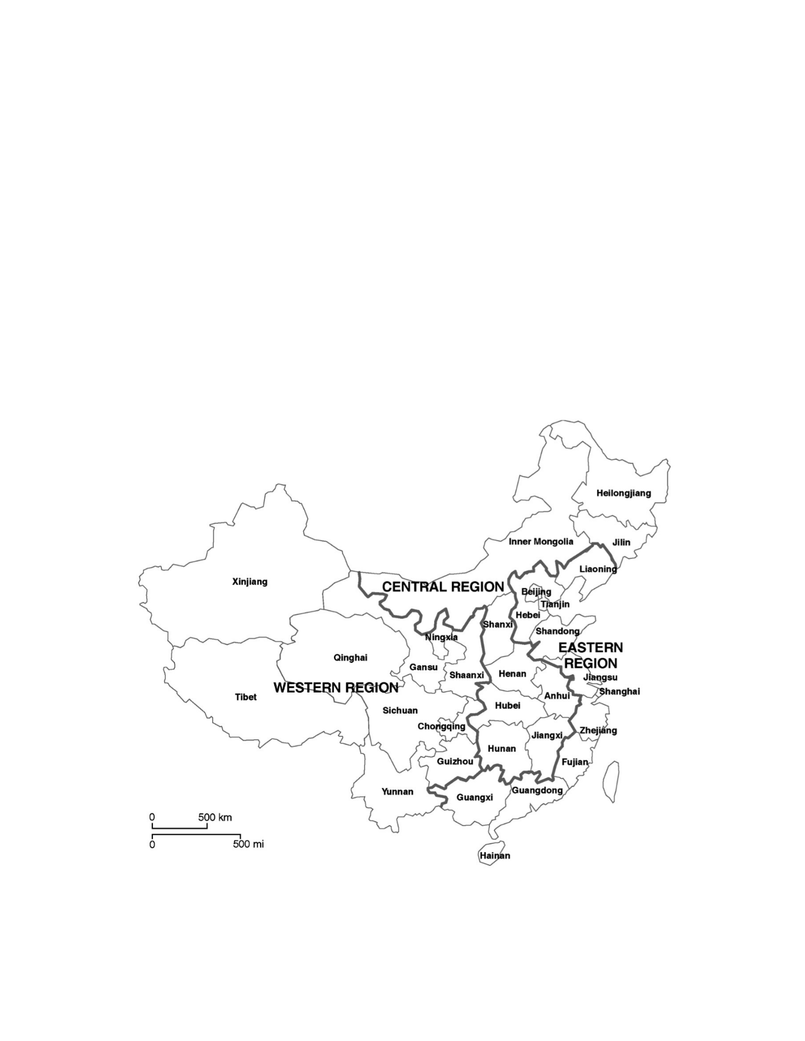
Central region includes eight provinces (Anhui, Henan, Heilongjiang, Hubei, Hunan, Jiangxi,

Jilin, and Shanxi) and one autonomous region (Inner Mongolia). The Eastern region includes

eight provinces (Fujian, Guangdong, Hainan, Hebei, Jiangsu, Liaoning, Shandong, and

Zhejiang), three municipalities (Beijing, Shanghai, and Tianjin), and one autonomous region

(Guangxi). Tibet is often omitted in income inequality studies according to Zhang and Zhang

(2003) and Chen (2006) because of serious missing values and the lack of consistent GDP data;

therefore, I also excluded Tibet from my analysis to avoid issues that may arise because of

missing values.

Figure 2.1: Provincial Units in China

Control variables included in the empirical model were provincial GDP per capita,

international trade openness, and educational attainment to control for other factors that might

affect income disparities at the provincial level (Table 2.2). First, provincial GDP per capita was

added into the empirical model to control for the “Kuznets effect” of economic growth on

income inequality. Li and Gibson (2012), however, investigated the recent problematic issue

related to using a wrongly calculated GDP per capita. They found that some Chinese provinces

recently changed to use GDP per resident, while some provinces are still using GDP per

registered population. Thus, some people were double-counted because they were in the

denominator of the statistics of GDP per capita for two or more places. In fact, Li and Gibson

(2012) found that 26 million were double counted in recent statistics. In addition, Tsui (2007) and

Li and Gibson (2012) argued that GDP per capita is overinflated due to a surge in migration to

richer provinces. Second, as shown in Liang’s (2006) empirical model, the variable of trade

openness was employed to capture the provincial degree of integration to the world economy.

Numerous papers have exploited the impact of trade globalization on income inequality but its

impact on inequality is inconclusive (Winters, et al., 2004). Some papers argue that the degree of

openness toward a world economy is related to a reduction in income inequality (Faustino and

Vali, 2011; Jaumotte, et al., 2013). On the other hand, others support that trade liberalization

leads to an increase in income inequality (Rudra and Haggard, 2001; Mah, 2013). Lastly, as

suggested in previous literature, educational attainment was employed as a proxy for human

capital, which is measured by the share of the provincial population with schooling of college

and higher (Checchi, et al., 1999; Sylwester, 2002; Hendel, et al., 2005; Yang and Qiu, 2016).

Table 2.2: Overview of Variables

Variable

Dependent Variable

Definition

Gini

Financial Variables

The Gini coefficient

Financial intermediation /

GDP

Gross value added of the financial sector as a share of provincial GDP

Financial intermediation: value-added of financial intermediation is the

final results that are calculated at market prices and produced in a region

during a given period by all resident units engaged in the financial sector.

Deposit / GDP

The ratio of total deposit to provincial GDP

Total deposit is a form of credit by which firms, institutions,

organizations, or households can put money into banks and other credit

institutions.

Loan / GDP

Control Variables

The ratio of total loan to provincial GDP

Total loan is a form of credit by which banks and other credit institutions

provide funds.

Gini (-1) The lagged variable of the Gini coefficient

Ln (GDP per capita) The logarithm of provincial GDP / number of residents in the

province

Openness The ratio of the sum of exports and imports to provincial GDP

Education attainment The number of people with more than secondary schooling as a share of

the total population

In order for quantitative analysis to be conducted, quantitative measures of financial

development need to be constructed. The depth, size, accessibility, and soundness of the financial

sectors should be captured by the indicators of financial development. The measurements for

financial development in this paper included: 1) the ratio of financial intermediation to provincial

GDP; 2) the ratio of total deposits of the financial institutions to provincial GDP; and 3) the ratio

of total loans of the financial institutions to provincial GDP. Since traditional indicators for

financial development are not available for an analysis within a country, Boyreau-Debray (2003)

developed local indicators of financial intermediation. For example, some applied the ratio of M2

(Money supply) to GDP to proxy for financial development, but M2 is not available at the

provincial level in China. Thus, I borrowed one of these indicators, calculated as the ratio of total

deposits of the financial institutions to GDP, to quantify the total size of the financial institutions.

Secondly, the ratio of private credit to GDP was constructed by Beck et al. (2007) as an indicator

of financial development. However, since data on private credit are not available, the ratio of

loan extended by financial intermediation to provincial GDP was taken to measure financial

intermediation development (Qi, et al., 2003). Lastly, based on the econometric model suggested

by Liang (2003), I introduced an indicator of financial intermediation as the share of the financial

industry in provincial GDP to measure how the financial markets are efficiently accessible. When

financial markets are large enough, accessibility to financial markets increases. In turn, increased

accessibility enables financial markets to provide reliable information that decreases transaction

costs and, thus, boosts resource allocation efficiently.

Table 2.3 displays the summary statistics for the dependent and control variables in this

paper. Among the 24 provinces or municipalities, the average Gini coefficient was 0.435 in 2014

(Table 2.4), relatively much higher than 0.318, the average Gini coefficient for OECD countries.

Its maximum value is 0.568 (Table 2.4), which is the Gini coefficient of the Guizhou province in

western China in 2014. Surprisingly, as seen in Table 2.4, the averages of the Gini coefficient

rose from 0.332 to 0.435 from 1998 to 2014, while the standard deviations of the Gini coefficient

increased from 0.047 to 0.071. In addition, the maximum values of Gini coefficients was only

0.410 in 1998 but increased to 0.568 in 2014, while the minimum values of the Gini coefficients

are quite stable, from 0.229 in 1998 to 0.285 in 2014. Clearly, this shows that the level of

income inequality in China has been on the rise, even though Table 2.1 indicates rapid financial

development in China. Similarly, the average provincial GDP per capita was 7403.8 Yuan per

person in 1998, but climbed to 50876.9 Yuan per capita in 2014, with an increase in standard

deviation from 5245.39 in 1998 to 21153.27 in 2014 (Table 2.5).

Table 2.3: Summary Statistics

Variables Mean STD Min 1st quartile Median 3rd quartile Max

Gini

0.397

0.060

0.229

0.359 0.396 0.440

0.568

Lgdp_ca 9.72 0.845 7.768 9.038 9.725 10.415 11.513

Open 0.332 0.461 0.031 0.078 0.130 0.388 4.657

Edu

0.116

0.096

0.008

0.045 0.093 0.155 0.509

F_gdp

0.048

0.034

0.006

0.030 0.038 0.054 0.431

D_gdp

1.476

0.756

0.709

1.102 1.334 1.604 10.356

L_gdp 1.085 0.506 0.378 0.829 1.019 1.236 8.706

Note: The number of observations is 408 for raw variables.

Table 2.4: Details of the Gini coefficient

Mean STD Min 1st quartile Median 3rd quartile

Max

1998 0.332 0.046 0.229 0.300 0.332 0.362 0.410

1999 0.346 0.044 0.248 0.317 0.351 0.369 0.421

2000 0.370 0.053 0.256 0.345 0.362 0.411 0.456

2001 0.381 0.054 0.270 0.348 0.374 0.423 0.466

2002 0.394 0.055 0.265 0.368 0.389 0.439 0.478

2003 0.404 0.054 0.267 0.362 0.412 0.437 0.483

2004 0.398 0.052 0.289 0.359 0.399 0.433 0.483

2005 0.403 0.048 0.280 0.380 0.404 0.432 0.478

2006 0.406 0.050 0.276 0.382 0.404 0.441 0.490

2007 0.406 0.052 0.280 0.381 0.401 0.445 0.491

2008 0.408 0.049 0.296 0.377 0.409 0.444 0.486

2009 0.408 0.049 0.290 0.381 0.410 0.436 0.484

2010 0.394 0.049 0.274 0.371 0.393 0.421 0.476

2011 0.421 0.066 0.275 0.361 0.438 0.471 0.513

2012 0.417 0.060 0.281 0.375 0.424 0.456 0.508

2013 0.429 0.068 0.294 0.376 0.446 0.479 0.536

2014 0.435 0.071 0.285 0.385 0.451 0.480 0.568

Note: The number of observations is 24 for each year.

Table 2.5: Details of Provincial GDP per capita

Mean STD Min 1st quartile Median 3rd quartile

Max

1998 7403.8 5245.39 2364 4320.0 5346.5 9509.0 25206

1999 7896.1 5739.82 2545 4517.5 5628.0 10204.5 27071

2000 8688.8 6376.14 2759 4962.0 6007.5 11185.5 29671

2001 9491.9 6991.90 3000 5441.0 6546.5 11953.5 32201

2002 10513.7 7831.49 3257 6017.5 7259.5 12969.0 35329

2003 12032.3 8766.78 3701 6826.0 8771.5 14301.5 39128

2004 14257.8 10317.41 4317 8342.0 10320.0 16152.0 46338

2005 16451.0 11431.23 5052 9669.5 11963.0 18814.5 51474

2006 18773.9 12590.27 5750 11216.0 13692.5 21477.0 57310

2007 22518.5 14082.14 7878 13914.5 16814.0 26289.0 62041

2008 26370.9 14900.59 9855 17160.5 20174.0 33304.0 66932

2009 28382.8 15449.92 10971 18396.5 22197.0 37292.5 69165

2010 33618.1 16745.58 13119 22684.0 27104.5 43545.5 76074

2011 39732.1 18003.11 16413 27405.5 33253.5 50783.5 82560

2012 43568.5 18711.82 19710 30553.5 36489.0 55372.0 87475

2013 47524.9 19947.08 23151 33414.0 39261.0 60414.5 94648

2014 50876.9 21153.27 26433 35099.0 41241.0 64336.5 99995

Note: The number of observations is 24 for each year.

Another interesting issue is found in a review of the financial development indicators.

The heterogeneity across space was observed. In Table 2.6, for example, the ratio of the financial

intermediation to provincial GDP in 1998 was 0.051, averaged over all of the provinces in the

sample. The ratio spreads from 0.041 for the financially least developed provinces to 0.157 for

the most developed province in 2014, compared to 0.007 to 0.129 in 1998 . In addition, the ratios

of all of the provinces in Central China were under 0.070 in 2014 with a standard deviation of

0.010, but the average ratio for provinces in Eastern China was 0.080 in 2014, greater than all

provinces in Central China. The ratios of all provinces in Eastern China increased to 0.157 over

the sample period. Table 2.7 tells us that the standard deviation of D_GDP in the Eastern region

was 1.005 in 2014, while it was 0.370 and 0.196 in the Central and Western regions, respectively.

Similarly, in Table 2.8, the ratio of loan to provincial GDP in 1998 had a mean of 0.994 with a

standard deviation of 0.250 while the average ratio of loan to provincial GDP in 2014 was 1.266

with a standard deviation of 0.349 across provinces. This geographical variation in level of

financial development indicates the necessity to conduct a meaningful statistical analysis.

Table 2.6: Details of F_GDP

Region Year Mean STD Min 1st

quartile

Median 3rd

quartile

Max Obs.

Eastern 1998 0.055 0.043 0.007 0.036 0.036 0.048 0.129 9

2014 0.080 0.041 0.046 0.056 0.066 0.073 0.157 9

Central 1998 0.040 0.018 0.024 0.026 0.036 0.058 0.070 7

2014 0.050 0.010 0.041 0.043 0.047 0.050 0.070 7

Western 1998 0.056 0.025 0.026 0.038 0.047 0.083 0.087 8

2014 0.066 0.014 0.053 0.054 0.061 0.080 0.086 8

Overall 1998 0.051 0.031 0.007 0.032 0.043 0.064 0.129 24

2014 0.067 0.029 0.041 0.051 0.057 0.071 0.157 24

Table 2.7: Details of D_GDP

Region Year Mean STD Min 1st

quartile

Median 3rd

quartile

Max Obs.

Eastern 1998 1.299 0.656 0.709 0.917 1.042 1.554 2.804 9

2014 1.979 1.005 1.278 1.469 1.489 1.920 4.375 9

Central 1998 0.897 0.194 0.714 0.737 0.866 0.978 1.279 7

2014 1.381 0.370 0.913 1.184 1.261 1.510 2.098 7

Western 1998 1.086 0.195 0.815 0.945 1.078 1.221 1.381 8

2014 1.741 0.196 1.529 1.578 1.683 1.917 2.042 8

Overall 1998 1.111 0.446 0.709 0.840 0.959 1.221 2.804 24

2014 1.723 0.678 0.913 1.369 1.531 1.894 4.375 24

Table 2.8: Details of L_GDP

Region Year Mean STD Min 1st

quartile

Median 3rd

quartile

Max Obs.

Eastern 1998 0.935 0.282 0.615 0.706 0.793 1.144 1.315 9

2014 1.358 0.398 0.951 1.114 1.181 1.707 2.131 9

Central 1998 0.894 0.179 0.560 0.767 0.932 1.029 1.071 7

2014 0.973 0.186 0.779 0.841 0.877 1.091 1.288 7

Western 1998 1.149 0.212 0.848 0.934 1.228 1.316 1.385 8

2014 1.418 0.258 1.065 1.223 1.369 1.642 1.811 8

Overall 1998 0.994 0.250 0.560 0.782 0.934 1.228 1.385 24

2014 1.266 0.349 0.779 1.045 1.184 1.512 2.131 24

Figure 2.A (Appendix) presents scatterplots of income inequality against financial

development indicators across the Chinese provinces. Specifically, Figure 2.A.1 displays

scatterplots with all observations across the country from 1998 to 2014, while Figure 2.A.2

shows scatterplots based on the Eastern, Central, and Western regions. In Figure 2.A.1, each

scatterplot illustrates changes in the Gini coefficients against each of the indicators for financial

development with all observations in the sample. Each scatterplot clearly illustrates that the Gini

coefficients are negatively associated with F_GDP, D_GDP, and L_GDP, while their slopes

slightly differ. In addition, the scatterplots based on regional level (Figure 2.A.2) display a

negative association between income disparity and the financial development measures, while

individual provincial scatterplots reveal that, aside from Hebei in Eastern China, income

inequalities of each province are positively associated with one or more indicators of financial

development (Figure 2.A.3). In Central China, all provinces except Jiangxi have a positive

association between income inequality and financial development with steeper slopes than those

in Eastern China (Figure 2.A.1). The regional scatterplot in Figure 2.A.2 shows a positive

association between the Gini coefficients and the ratio of financial intermediation to provincial

GDP across Central China. In every province in Western China, the Gini coefficients are

positively correlated with at least one indicator of financial development (Figure 2.A.1). In

addition, income disparities in Western China are positively related with financial development,

while the change in income inequalities against the change in the ratio of loan to provincial GDP

has the highest slope among the indicators of financial development (Figure 2.A.2).

2.3.2 Financial Development Over Time in China

While China’s economic reforms have been successful in moving to a socialist market

economy and spurring impressive growth rates, China’s financial system is less efficient as four

major state-owned banks have more than 60% of the total financial assets in the Chinese

economy. As an initial effort for financial reform, the People’s Bank of China separated from the

Ministry of Finance in 1978. In the following year, China re-established the Bank of China, the

People’s Construction Bank of China, and the Agricultural Bank of China to create free

competition and market forces in their lending services and savers. In 1983, the Chinese

government designated the People’s Bank of China as a central bank and set up the Commercial

Bank to allow for more convenient financial service. Three national banks (Everbright, Hua Xia,

and Min Sheng), many regional banks, and different non-bank financial service suppliers, which

increased the accessibility to financial assets, were established at the end of the 1980s. China has

significantly changed the lending policy for state own enterprises (SOE) so that the ratio of

SOE’s dependency on direct government transfers reduced to 2% in the early 1990s, while the

ratio of bank finance not provided by government transfers rose to 32% between 1980 and 1987.

The second major transition in the financial sector took place between 1994 and 2000. In

1994, China established three policy banks, initiated indirect monetary control, and enacted the

Commercial of Bank of China to operate commercial banks efficiently. In 1998, China

terminated credit planning, which was set up for commercial banks owned by the state.

Remarkably, China allowed the first private-owned bank (China Minsheng Bank) and 13

jointstock commercial banks to enter the Chinese banking sector by early 2000.

In the history of financial development in China, entry into the WTO in December 2001

brought the greatest changes to China’s financial system. Joining the WTO forced China to take

more aggressive policies in interest rate liberalization, deregulation on foreign banks and

investors, and the easing of property rights to attract more foreign banks. In 2003, the China

Banking Regulatory Commission (CBRC) was founded to regulate the banking sector and

further promote asset quality, risk control, and capital adequacy. Notably, according to Wang and

Zhang (2009), since the CBRC encouraged foreign banks to enter the Chinese domestic banking

sector and forced all new commercial banks to have at least one foreign investor, a total of 223

foreign banks from 42 countries entered the domestic banking sector by 2006.

2.4 Model

Before setting up the empirical model, a statistical hypothesis test is needed to determine

whether each of the financial development measures in the empirical model is useful in

forecasting the Gini coefficient or whether the Gini coefficient has an impact on financial

development rather than the other way around. For this reason, the Granger Causality Test was

applied, and its results are shown in Table 2.9. I reject the null that the ratio of financial

intermediation to provincial GDP does not granger cause the Gini coefficient while failing to

reject the null that the Gini coefficient does not granger cause the ratio of financial

intermediation to provincial GDP, suggesting unidirectional causality from the ratio of financial

intermediation to provincial GDP to the Gini coefficient. In addition, I reject the null that the

ratio of total deposit to provincial GDP does not granger cause the Gini coefficient, while failing

to reject the null that the Gini coefficient does not granger cause the ratio of total deposit to

provincial GDP, indicating unidirectional causality from the ratio of total deposit to provincial

GDP to the Gini coefficient. This means that financial development measured by these two ratios

causes the changes in income disparities measured by the Gini coefficient. Therefore, for these

two financial development measures, unidirectional causality from financial development

measures to the Gini coefficients is captured using the Granger Causality Test.

For the ratio of total loan to provincial GDP, however, I fail to reject both null hypotheses

that the ratio of total loan to provincial GDP does not granger cause the Gini coefficients. Wei

(2016) argued that banks in China intentionally hide more than $2 trillion in loans, reporting that

Chinese banks keep the loan spigot open to stimulate Chinese economy growth, which has begun

to slow down gradually since 2010. Loans are repackaged as “investment receivables” so that a

surge in the loans could be included as “investment receivables” in banks’ balance sheets.

According to this argument, I assume that the collected loan data could be possibly less credible

and, therefore, the ratio of total loan to provincial GDP does not granger cause the Gini

coefficients even though it is frequently used to measure financial development.

Table. 2.9: Granger Causality Test

Null Hypothesis F-statistic

f_gdp does not granger cause Gini 2.27*

Gini does not granger cause f_gdp 0.28

d_gdp does not granger cause Gini 4.22***

Gini does not granger cause d_gdp 1.93

l_gdp does not granger cause Gini 1.70

Gini does not granger cause l_gdp 0.79

Note: Data span for Granger Causality Test: 1995-2014

***, **, and * indicates significance at the 1%, 5%, and 10% level, respectively

Having established the direction of causality, I now turn to the main research question,

which is how income disparities are related to financial development after controlling for GDP

per capita, the degree of openness, and educational attainment. To solve this main empirical

question, the following estimation equation is needed.

giniit =β1Fit' +β2 Xi't +ui +eit (4)

Here, Giniit is the Gini coefficient in province i and year t. Gini is a general measure of statistical

dispersion showing income distribution and is the most frequently used measure of income

inequality. Fit , which is the focus of my analysis, is one of the following financial development

indicators: 1) the ratio of the value added in financial intermediation to provincial GDP or the

ratio of financial intermediation to provincial GDP (f_gdp), where the value-added of financial

intermediation is the final result that is calculated at market prices and produced in a province

during a given period by all residents engaged in finance; 2) the ratio of total deposit of the

financial institution to provincial GDP (d_gdp); and 3) the ratio of loans extended by financial

intermediation to provincial GDP (l_gdp). The vector Xit contains the set of control variables: 1)

the logarithm of provincial GDP per capita (lgdp_ca), which controls for a Kuznets effect of

economic development on income disparities; 2) the degree of provincial economic openness to

foreign countries (open) as measured by the ratio of the sum of exports and imports to provincial

GDP; and 3) educational attainment (edu), the share of the population with more than secondary

schooling as a proxy for education development. Additionally, this empirical model includes ui ,

which is a provincial random effect and eit, which is an error term. In equation (4), β1 and β2 are

parameters. The effect of financial development on income inequality is captured by the

parameter β1, whereas the overall level of income disparity is captured by all of the variables on

the right hand side of equation (4). When estimating the empirical model (4), it turns out that the

assumptions of standard fixed effects model are violated and that residuals are serially correlated

even if the variables in the model are first-differenced. To resolve this statistical issue, the lagged

dependent variable is included in the empirical model (4):

giniit =β0giniit−1 +β1Fit' +β2 Xi't +ui +eit (5)

The GMM is the most commonly used technique when there is endogeneity among the

lagged dependent variables in panel data models. The explanatory variables on the right-hand

side of the equations may be associated with the error term or with the province specific error

component. Furthermore, the model has the lagged dependent variables on the right-hand side of

the equations, inserting to autocorrelation. Lastly, a possible problem is the short time period (18

years) in the dataset. Therefore, the Ordinary Least Square (OLS) estimators will be biased and

inconsistent. Arellano and Bond (1991) mentioned that if the errors are serially correlated, an

estimator that uses lagged instruments under the assumption of white noise errors loses its

consistency. They applied these methods to estimate employment equations using an unbalanced

panel of 140 listed U.K. companies for the period from 1979 to 1984. The estimator also had

significant efficiency gains compared to simpler instrument variable (IV) estimator and produced

well determined estimates in dynamic panel data models. As suggested by Holtz et al. (1988) and

Arellano and Bond (1991), the first difference GMM estimator is frequently utilized to deal with

the endogeneity in panel data to eliminate individual fixed effects from the equation.

However, Bond et al. (2001) pointed out that the first-differenced GMM estimators tend to

behave poorly -- exhibiting seriously bias due to the weakness of the instruments for the

firstdifferences -- when the number of time series is moderately small and the time series are

persistent. This bias can decrease if the time span is large enough (Nickell, 1981), but the data in

this study is only18 years. Thus, I turn to the so called system GMM estimation approach. In

order to improve the properties of the standard first-differenced GMM estimator, the system

GMM estimator is developed when the lagged levels of the explanatory variables are poor

instruments for the first-differenced explanatory variables on the right hand side of the equation.

To improve efficiency, the system GMM estimator utilizes the level equation in addition to the

differenced equation, and the variables in levels in the second equation are instrumented with

lagged first-differences of the endogenous variables (Arellano and Bond, 1991; Arellano and

Bover, 1995; Blundell and Bond, 1998). Specifically, in the case where the number of time series

(N) is small and time period (T) is long, the first differenced GMM estimators are not

appropriate (Roodman, 2007). To deal with this issue, Blundell and Bond (1998) added an extra

restriction on the initial conditions process to improve the precision of the first-differenced

GMM estimator for dynamic panel data models. By means of Monte Carlo simulations, they

showed that the system GMM estimator yields greater precision relative to the standard

firstdifferenced GMM estimator when the autoregressive parameter is high and the number of

time series is small.

2.5 Empirical Results

Table 2.10 presents the empirical results based on equation (5) with Chinese provincial

data from 1998 to 2014 to investigate how income inequalities are associated with financial

development. Columns (1), (2), and (3) in Table 2.10 indicate the results from OLS without

controlling for the endogeneity of the financial development measures. In OLS estimations, none

of financial development measurements are significant. In system GMM estimations, however,

there are strong relations between financial development and income inequality, with increases in

two financial development indicators (f_gdp and l_gdp) being significantly associated with

increases in Gini coefficients. First, the coefficient on the ratio of financial intermediation to

provincial GDP is positive and statistically significant at the 5% level in column (4) of Table

2.10, suggesting that a 1 unit increase in the ratio of financial intermediation to provincial GDP

increases the Gini coefficient by 14.90. Column (5) shows that the coefficient on the deposit to

provincial GDP is positive but not significant. Lastly, the ratio of loan to GDP is positively

associated with income inequality at the 1% significance level, suggesting that an increase in

loan to provincial GDP by 1 unit is associated with an increase in the Gini coefficient by 1.18.

As for the control variables, income inequalities are thought to be causally tied to provincial

GDP per capita. The coefficients on the provincial GDP per capita are positively significant in

the GMM model, while those are insignificant in pooled OLS. The coefficients on the degree of

openness are negative and statistically significant at the 1% significance level, for the columns

(4) and (6) in the GMM estimation. The coefficients on education attainment are negatively

significant, which conforms to general expectation that higher education attainment leads to a

reduction in inequality.

Table 2.10: Financial Development and Income Inequality Based on Equation (5):

(Dependent variable: Gini Coefficient)

Variables Pooled OLS GMM

Financial

variables

(1)

(2)

(3)

(4)

(5)

(6)

F_gdp 5.61

(1.28)

14.90**

(2.55)

D_gdp 0.08

(0.37)

0.32

(1.01)

L_gdp 0.30

(1.16)

1.18***

(3.32)

Control

variables

Gini (-1) 0.91***

(43.55)

0.90***

(41.79)

0.90***

(41.81)

0.79***

(30.97)

0.78***

(31.11)

0.77***

(30.65)

Lgdp_ca 0.03

(0.13)

0.03

(0.15)

0.07

(0.34)

0.61**

(2.28)

0.93***

(3.58)

0.87***

(3.40)

Open -0.41

(-1.24)

-0.25

(-0.70)

-0.40

(-1.19)

-2.13*** (-

4.10)

-1.58** (-

2.49)

-2.61*** (-

4.38)

Edu -4.85*** (-

2.73)

-4.61** (-

2.25)

-4.74*** (-

2.68)

-7.04** (-

2.50)

-10.67*** (-

3.85)

-8.17*** (-

2.95)

Cons 4.57***

(2.69)

4.61**

(2.56)

4.26**

(2.42)

3.74*

(1.94)

1.53

(0.80)

1.85

(0.98)

Adj. R2 0.884 0.883 0.883

Arellano-

Bond test (2) 2.11 2.15 2.01

Sargan test

(P-value)

390.44

(0.29)

389.75

(0.30)

383.93

(0.38)

# of Obs. 384 384 384 384 384 384

Note: ***, **, and * indicates significance at the 1%, 5%, and 10% level, respectively. The numbers in parentheses

are t-statistics for pooled OLS and z-statistics for GMM. Arellano-Bond Test (for AR (2)) is for autocorrelation with a

null hypothesis of no autocorrelation. Sargan test’s null hypothesis is that over-identifying restrictions are valid.

Next, a dummy variable for WTO membership, equal to 1 only in a given year, is added

into equation (5) to investigate how entry into the WTO affected the income inequality in China.

In other words, it allows us to examine whether becoming a WTO member has a short-term

shock to the economic system. The GMM estimators in Table 2.11 indicate that the ratios of

financial intermediation to GDP and loan to GDP are positively significant at the 1%

significance level, suggesting that income inequality measured by Gini coefficients turns out to

have increased over the sample period with a more developed financial system. More

interestingly, the size of the estimated slopes on the indicators of financial development

increased slightly from 14.90 to 15.21 for f_gdp and from 1.18 to1.19 for l_gdp. The estimated

slopes on the WTO membership dummy, however, are not statistically significant. As for

the control variables, the impacts of the degree of openness toward a world economy do not

differ much from previous results in Table 2.10. Similarly, Table 2.11 shows that the size of the

coefficients on degree of openness increased slightly. The size of the estimated slopes on the

degree of openness increased from -2.13 to -2.16 in column (1) and from -2.61 to -2.63 in

column (3). In addition, GDP per capita is positively associated with income inequality for all

columns in Table 2.11. Lastly, educational attainment has a negative and significant effect on

income inequality in column (1), suggesting an increase in educational attainment by 1 unit is

related to a decrease in the Gini coefficient by 7.01.

Alternatively, another type of WTO membership dummy, which equals to 1 if the year is

greater than 2001, is created to analyze whether being a WTO member has a long-term shock to

Chinese economy. The size of the estimated slopes on financial indicators slightly increased from

15.21 (column 1) to 17.14 (column 4) and from 1.19 (column 1) to 1.20 (column 4). Overall, the

impacts of the control variables from being a WTO member do not differ much from becoming a

member. The estimated slopes on the WTO membership dummy, however, are still

not statistically significant.

Table 2.11: Financial Development and Income Inequality Based on Equation (5):

With WTO membership dummy (Dependent variable: Gini coefficient)

1 if year = 2001 1 if year > 2001

Financial var. (1)

(2)

(3)

(4)

(5)

(6)

F_gdp 15.21***

(2.59)

17.14***

(2.74)

D_gdp 0.33

(1.02)

0.32

(1.00)

L_gdp 1.19***

(3.35)

1.20***

(3.36)

Control var.

Gini (-1) 0.79***

(30.89)

0.78***

(31.00)

0.77***

(30.51)

0.78***

(25.56)

0.78***

(25.94)

0.76***

(25.09)

Lgdp_ca 0.58**

(2.17)

0.92***

(3.50)

0.85***

(3.30)

0.59**

(2.22)

0.93***

(3.56)

0.87***

(3.40)

Open -2.16*** (-

4.14)

-1.60** (-

2.50)

-2.63*** (-

4.41)

-2.28*** (-

4.23)

-1.58** (-

2.48)

-2.64*** (-

4.40)

Edu -7.01** (-

2.49)

-10.66*** (-

3.85)

-8.14*** (-

2.94)

-7.86*** (-

2.68)

-10.57*** (-

3.61)

-8.51*** (-

2.94)

WTO membership

Dummy

-0.18

(-0.54)

-0.10

(-0.30)

-0.17

(-0.50)

0.31

(0.95)

-0.02

(-0.07)

0.13

(0.44)

Cons 3.99**

(2.01)

1.66

(0.85)

2.07

(1.07)

4.34**

(2.15)

1.51

(0.77)

2.08

(1.07)

Arellano-

Bond test (2)

2.10 2.15 2.01 2.12 2.20 2.12

Sargan test (P-

value)

390.41

(0.28)

389.36

(0.29)

383.86

(0.36)

394.80

(0.24)

388.21

(0.32)

385.60

(0.36)

# of Obs. 384 384 384 384 384 384

Note: ***, **, and * indicates significance at 1%, 5%, and 10% level, respectively. The numbers in parentheses are z-

statistics.

To check the robustness of the empirical results, alternative specifications were

examined. First, a regional dummy was employed as an additional explanatory variable because

Eastern provinces received greater attention of Chinese economic development policies and of

foreign investors, while Western and Central provinces fell behind in their development. The

Eastern provinces grew quickly, while the Central and Western provinces lagged behind. Lee

(2000) discussed that the sources of Chinese inequality have changed from within provinces to

between provinces. Therefore, I re-estimated equation (5), adding a regional dummy for Eastern

provinces to assess this particular omitted variable bias, which may cause a spurious relationship

between financial variables and the Gini coefficient. Table 2.12 reports the empirical results

including a regional dummy for Eastern provinces (1= Eastern, 0 otherwise). Looking at the

impact of the region dummy, all columns indicate region dummies for Eastern provinces are

statistically significant at the 1% significance level, suggesting average Gini coefficients in

Eastern provinces are 2.42 point to 3.25 point less than Central and Western provinces. Financial

development (loan to provincial GDP) also affected income inequality over the sample period.

After adding a regional dummy for Eastern provinces, the coefficient of the ratio of loan to

provincial GDP is still positive and statistically significant at the 10% significance level. Overall

directions and sizes of coefficients on financial development measurement are not much different

from the initial estimation results in Table 2.10.

Table 2.12: Robustness check 1: Regional dummy (Dependent

variable: Gini coefficient)

Variables Region dummy: 1 = Eastern, 0 Otherwise

Financial variables (1) (2) (3)

F_gdp 6.33

(1.06)

D_gdp -0.16

(-0.50)

L_gdp 0.72*

(1.95)

Control variables

Gini (-1) 0.73***

(25.24)

0.72***

(25.09)

0.72***

(25.10)

Lgdp_ca 0.79*** (3.04) 0.98

(3.91)

0.98***

(3.90)

Open -0.73

(-1.21)

-0.02

(-0.03)

-1.36** (-

1.97)

Edu -7.01*** (-

2.58)

-8.51

(-3.14)

-8.23***

(-3.06)

Dummy region -2.88*** (-

4.20)

-3.25*** (-

4.20)

-2.42***

(-3.33)

Cons 5.43*** (2.85) 4.76**

(2.40)

3.79**

(1.97)

Arellano-Bond test for AR (2) 2.11 2.11 2.03

Sargan test 402.53

(0.16)

404.46

(0.14)

396.03

(0.22)

# of Obs. 384 384 384

Note: ***, **, and * indicates significance at the 1%, 5%, and 10% level, respectively. The numbers in parentheses

are z-statistics.

Second, I dropped the educational attainment variable from the vector of control

variables. Generally, educational attainment is known as a function of economic growth rate

(Sardadvar, 2012). In other words, the empirical models for financial development and economic

growth include educational attainment as an explanatory variable on the right-hand side of the

equation and the Gini coefficient as a dependent variable. Thus, the reduced form of equation (5)

excluding educational attainment allows us to take away colinearity. Table 2.13 shows the

empirical results from the reduced form of equation (5) and reveals that financial development

still has a significant positive effect on income inequality, suggesting an increase in the ratio of

financial intermediation to provincial GDP by 1 point is associated with an increase in inequality

by about 16.09 and a 1point increase in the loan to provincial GDP ratio leads to a 1.17 increase

in inequality.

Table 2.13: Robustness check 2: Excluding educational attainment (Dependent

variable: Gini coefficient)

Financial variables (1) (2) (3)

F_gdp 16.09***

(2.68)

D_gdp 0.12

(0.37)

L_gdp 1.17***

(3.28)

Control variables

Gini (-1) 0.77*** 0.78*** 0.74***

(28.69) (30.46) (28.14)

Lgdp_ca 0.22

(1.41)

0.28*

(1.87)

0.45***

(3.03)

Open -1.13***

(-4.09)

-1.36** (-

2.03)

-2.64***

(-4.42)

Cons 7.39***

(6.16)

7.00***

(5.82)

5.97***

(4.91)

Sargan test 387.06 385.81 379.19

(P-value) (0.17) (0.18) (0.23)

# of Obs. 384 384 384

Note: ***, **, and * indicates significance at the 1%, 5%, and 10% level, respectively. The numbers in parentheses

are z-statistics.

Lastly, to test the robustness of the estimation results, I exclude two municipalities of

Beijing and Shanghai since the banking sector in these cities is impacted by fewer policy loans

from the central bank and has a heavily diversified banking sector. In addition, the top 10 ranked

universities in China are heavily weighted in favor of Beijing (Tsing Hua University, Peking

University, and Renmin University) and Shanghai (Fudan University; Shanghai Jiao Tong

University), which may affect educational attainment. More importantly, the size of Beijing and

Shanghai is much smaller than other provinces in the dataset, which may cause less policy lag

than other provinces when implementing local policy to reduce income disparities. Dropping

Beijing and Shanghai, cities that are extremely biased toward financial and educational

development, enables us to check whether there exists a case of sample heterogeneity, which

may arise if Beijing and Shanghai behave differently. The estimation results after dropping

Beijing and Shanghai are presented in Table 2.14. These results are largely similar to results

when Beijing and Shanghai are included in the dataset (Table 2.10), indicating financial

development increases income inequality. The main differences are found in column (1) and (2):

First, the estimated slope of f_gdp is increased to 25.69; second, it turns out that the ratio of

deposit to provincial GDP has a significant positive effect on income inequality, suggesting an

increase in this ratio by 1 point is related to an increase in income inequality by about 0.95 point.

Next, I integrate Beijing and Shanghai into Hebei and Zhejiang respectively instead of simply

dropping those two municipalities. To incorporate to the provinces, the weighted average values

of each variable are calculated and replaced with the initial values of variables in the dataset

based on the equation (6) of Appendix. Overall, as shown on Table 2.14, the estimation results

from dropping Beijing and Shanghai are not much different from integrating those municipalities

into each province. Therefore, the estimating model excluding or including

Beijing and Shanghai does not seem to create considerable differences.

Table 2.14: Robustness check 3: Excluding the municipalities (Beijing

and Shanghai)

Dropping Beijing and Shanghai Integrating Beijing to Hebei and

Shanghai to Zhejiang

Financial var. (1)

(2)

(3)

(4)

(5)

(6)

F_gdp 25.69***

(4.03)

22.53***

(3.55)

D_gdp 0.95***

(2.68)

0.80**

(2.31)

L_gdp 1.47***

(3.93)

1.63***

(4.53)

Control var.

Gini (-1) 0.75***

(26.22)

0.74***

(26.21)

0.73***

(25.87)

0.76***

(26.60)

0.75***

(26.56)

0.73***

(25.55)

Lgdp_ca 0.20

(0.64)

0.44

(1.48)

0.56*

(1.93)

0.38

(1.18)

0.64**

(2.08)

0.79**

(2.61)

Open -2.58*** (-

4.39)

-2.36*** (-

3.27)

-2.86***

(-4.25)

-2.48*** (-

4.32)

-2.33*** (-

3.26)

-3.19*** (-

4.97)

Edu 0.07

(0.02)

-2.82

(-0.77)

-2.10

(-0.58)

-2.65

(0.70)

-5.70

(-1.55)

-5.04

(-1.36)

Cons 8.67***

(3.61)

6.40***

(2.71)

5.52**

(2.41)

6.84***

(2.82)

4.71**

(2.02)

3.71

(1.60)

Arellano-Bond

test for AR (2)

1.83 1.87 1.82 1.88 1.94 1.83

Sargan test (P-

value)

374.48

(0.22)

378.84

(0.17)

369.55

(0.27)

377.19

(0.19)

380.75

(0.16)

373.20

(0.23)

# of Obs. 352 352 352 352 352 352

Note: ***, **, and * indicates significance at the 1%, 5%, and 10% level, respectively. The numbers in parentheses

are z-statistics.

2.6 Conclusion

Previous theoretical studies provide remarkably dynamic models to investigate the link

between financial development and income inequity by offering theoretical consensus that the

poor or low-income labor receive benefits from financial deepening. There is a lack of empirical

studies that examine the theoretical financial development ─ inequality relationship, particularly

for income disparities in China due to a lack of accessible data at the province, city, and county

levels, even though a surge in overall national inequality is attributed to an increase in income

inequality within provinces, cities, or counties across the country. In this paper, based on a recent

dataset between 1998 and 2014, I explored the long-run relationships between financial

development and income inequality by looking at how income disparities are associated with

financial development. First, one of main findings is that the ratio of financial intermediation to

provincial GDP has a significant positive impact on income inequality, and it is robust across all

specifications. Second, the empirical model with the year dummy for 2001 to explore the effect

of entry into the WTO reports that the positive impacts of financial development on income

inequality increased, indicating entry into the WTO accelerated financial development in China.

Lastly, the specification with the region dummy for Eastern provinces reveals that these

provinces, which received greater attention of Chinese economic development policies and of

foreign investors, are more equal than other provinces. As for educational attainment, initially, its

effect on inequality is negatively significant as expected. After dropping Beijing and Shanghai,

however, educational attainment is no more significant. However, it differs from the general

thought that increasing educational attainment leads to a reduction in income inequality. This

disjunction can be explained by educational inflation or devaluation of educational attainment in

Chinese education, where the number of people who graduated from Chinese higher education

increased from 1 million per year in 2000 to 7 million per year in 2010, and total enrollment of

students in higher educational institutions increased to 15 million, with rapid growth that was

expected to peak in 2008 (Caron, 2012; Porter, 2005). According to Robbins (2016), the Chinese

government evaluated national universities in 1994, and through Project

985 and the Thousand Talents Program11, they reformed the higher education system with an

emphasis on elite universities. Consequentially, the Chinese government adopted an advanced

education system in some of the elite institutions, such as Peking University and Tsinghua

University, for selected students. As discussed, education reform was extremely radical to foster

some of the selected elite universities, which reveals why educational attainment is losing its

impact on reducing income inequality.

This study has the following policy implication. Financial development policy subsidized

by local or provincial government spending such as a low-interest loan, micro finance, or

subsidized education loans, will enhance the number of lending activities of low-income people

and therefore lead a reduction in income disparities. While financial development, which is

seriously biased toward Eastern provinces, promotes economic growth in China, Gini

coefficients in the provincial level have been increased even though overall Chinese Gini

coefficient has been decreased. Along with huge economic growth driven by economic reforms

since 1978, China has successfully decreased overall income inequality and poverty line.

However, its central government policy such as government expenditures is biased toward

urbanization and infrastructural construction not towards social safety net or unemployment care.

Easterlin et al. (2012) reported that the degree of life satisfaction among the Chinese decreased

from 1990 to 2010. Although China has achieved enormous economic growth with an average

annual growth rate of 10%, the achievement of hyper-growth has led to income inequality. An

increase in interprovincial inequality may lead to socioeconomic instability, which can be an

obstacle in China’s economic growth in the long run. For long-term economic growth viability, it

is necessary to organize a reliable interprovincial level dataset and, furthermore, a city or county

level dataset to reveal the determinants of interprovincial income

11 This is a talent recruitment program conducted by the Chinese government in 2008 to recruit talented professors

and researchers for universities and institutions in China.

inequality with polygonal angles. This will enable us to reveal fundamental causes of income

inequality in China, to explore the dynamics of income disparities, and to examine newly

contributing factors.

2.A Appendix

Table 2.A.1: Panel Data Model Estimations between1998 and 2014 (Dependent

Variable: Gini Coefficient)

Random Effect GLS without gini (-1) Random Effect GLS with gini (-1)

F_gdp -29.30*** (-

3.09)

5.61

(1.28)

D_gdp 0.72

(1.28)

0.08

(0.37)

L_gdp 0.99

(1.62)

0.30

(1.16)

Gini (-1) 0.91***

(43.55)

0.90***

(41.79)

0.90***

(41.81)

Lgdp_ca 3.29***

(7.64)

3.03***

(7.03)

3.09***

(7.23)

0.03

(0.13)

0.03

(0.15)

0.07

(0.34)

Open 1.78*

(1.95)

-1.64

(-1.40)

-1.78*

(-1.65)

-0.41

(-1.24)

-0.25

(-0.70)

-0.40

(-1.19)

Edu -3.72

(-0.68)

-0.35

(-0.35)

-0.94

(-0.17)

-4.85*** (-

2.73)

-4.61** (-

2.25)

-4.75*** (-

2.68)

Intercept 9.01**

(2.45)

9.92***

(2.69)

9.32**

(2.52)

5.61***

(2.69)

4.61***

(2.56)

4.26**

(2.42)

Obs. 408 408 408 384 384 384

Note: ***, **, and * indicate significance at the 1%, 5%, and 10% level, respectively. The numbers in parentheses

are z-statistics.

Table 2.A.2: Panel Data Model Estimations between 1998 and 2014

(Dependent Variable: Gini Coefficient)

Fixed Effect without gini (-1) Fixed Effect with gini (-1)

F_gdp -33.77*** (-

3.64)

4.09

(0.55)

D_gdp 0.15

(0.24)

-0.16

(-0.35)

L_gdp -0.15

(-0.23)

0.43

(0.93)

Gini (-1) 0.66***

(16.43)

0.65***

(16.61)

0.65***

(16.65)

Lgdp_ca 2.59***

(5.87)

2.10***

(4.60)

2.15***

(4.95)

0.46

(1.28)

0.56

(1.58)

0.49

(1.43)

Open 3.21***

(3.46)

0.33

(0.25)

0.86

(0.73)

-0.25

(-0.34)

0.40

(0.39)

-0.62

(-0.71)

Edu 8.62

(1.48)

2.53**

(2.53)

14.20**

(2.43)

2.40

(0.52)

1.42

(0.31)

2.63

(0.58)

Intercept 14.03***

(3.83)

17.23***

(4.64)

17.04***

(4.69)

9.34***

(3.24)

8.82***

(3.06)

8.99***

(3.18)

Obs. 408 408 408 384 384 384

Note: ***, **, and * indicate significance at the 1%, 5%, and 10% level, respectively. The numbers in parentheses

are t-statistics.

Table 2.A.3: Panel Data Model Estimations between 1998 and 2014

(Dependent Variable: Gini Coefficient)

Random MLE without gini (-1) Random MLE with gini (-1)

F_gdp -33.06*** (-

3.65)

5.61

(1.29)

D_gdp 0.26

(0.44)

0.08

(0.38)

L_gdp 0.12

(4.00)

0.30

(1.17)

Gini (-1) 0.91***

(43.90)

0.90***

(42.12)

0.90***

(42.14)

Lgdp_ca 2.77***

(6.43)

2.32***

(5.25)

2.36***

(5.55)

0.03

(0.14)

0.03

(0.15)

0.07

(0.34)

Open 2.93***

(3.24)

-0.07

(-0.06)

0.24

(0.21)

-0.41

(-1.25)

-0.25

(-0.70)

-0.40

(-1.20)

Edu 5.66

(1.00)

11.08*

(1.94)

10.82*

(1.90)

-4.85*** (-

2.75)

-4.61

(-2.27)

-4.75*** (-

2.70)

Intercept 12.77***

(3.35)

15.55***

(3.86)

15.27***

(4.00)

4.57***

(2.71)

4.61***

(2.58)

4.26**

(2.43)

Obs. 408 408 408 384 384 384

Note: ***, **, and * indicate significance at the 1%, 5%, and 10% level, respectively. The numbers in parentheses are

z-statistics.

∗! "#

Equation (6): Integrating Beijing to province Hebei and Shanghai to province Zhejiang

1. 𝐺𝑖𝑛𝑖!"#$#%&!!"#"$ = 𝐺𝑖𝑛𝑖!"#$#%& !"#$%&’(")!"#$#%&!!"#"$

𝐺𝑖𝑛𝑖!"#"$ ∗ !"#$%&’("!"#$%&’(")!"#$#%&)!"#"$!!"#"$

2. 𝐹_𝑔𝑑𝑝!"#$#%&!!"#!" =𝐹_𝑔𝑑𝑝!"#$#%& !"#!"#$#%&!!"#"$ +𝐹_𝑔𝑑𝑝!"#"$ ∗

!"#!!"#"#$#%&!"#"$!!"#"$

3. 𝐷_𝑔𝑑𝑝!"#$#%&!!"#"$ =𝐷_𝑔𝑑𝑝!"#$#%& !"#!"#$#%&!"#$#%&!!"!"# +𝐷_𝑔𝑑𝑝!"#"$ ∗!

"#!!"#"#$#%&!"#"$!!"#"$

4. 𝐿_𝑔𝑑𝑝!"#$#%&!!"#"$ =𝐿_𝑔𝑑𝑝!"#$#%& ∗! "#!!"#"#$#%&!"#$#%&!!"#"$

+𝐿_𝑔𝑑𝑝!"#"$ ∗!"#!!"#"#$#%&!"#"$!!"#"$

5. 𝐿𝑔𝑑𝑝_𝑐𝑎!"#$#%&!!"#"$

𝑃𝑜𝑝𝑢𝑙𝑎𝑡𝑖𝑜𝑛!"#$#%& 𝑃𝑜𝑝𝑢𝑙𝑎𝑡𝑖𝑜𝑛!"#"$

=𝐿𝑔𝑑𝑝_𝑐𝑎!"#$#%& ∗ 𝑃𝑜𝑝𝑢𝑙𝑎𝑡𝑖𝑜𝑛!"#$#%&!!"#"$ +𝐿𝑔𝑑𝑝_𝑐𝑎!"#"$ ∗

𝑃𝑜𝑝𝑢𝑙𝑎𝑡𝑖𝑜𝑛!"#$#%&!!"#"$

6. 𝑂𝑝𝑒𝑛!"#$#%&!!"#"$ =𝑂𝑝𝑒𝑛!"#$#%& ∗! "#!!"#"#$#%&!"#$#%&!!"#"$

+𝑂𝑝𝑒𝑛!"#"$ ∗! "#!!"#"#$#%&!"#"$!!"#"$

7. 𝐸𝑑𝑢!"#$#%&!!"#"$ =𝐸𝑑𝑢!"#$#%& ∗ !"#$%&’("!"#$%&’(")!"#$#%&)!"!"!

#$!!"#"$ +𝐸𝑑𝑢!"#"$ ∗ !"#$%&’("!"#$%&’(")!"#$#%&)!"#"$!!"#"$

Figure 2.A.1: The Scatterplots with all observations across a country (Y-axis:

Gini, X-axis: Each of the measures of financial development)

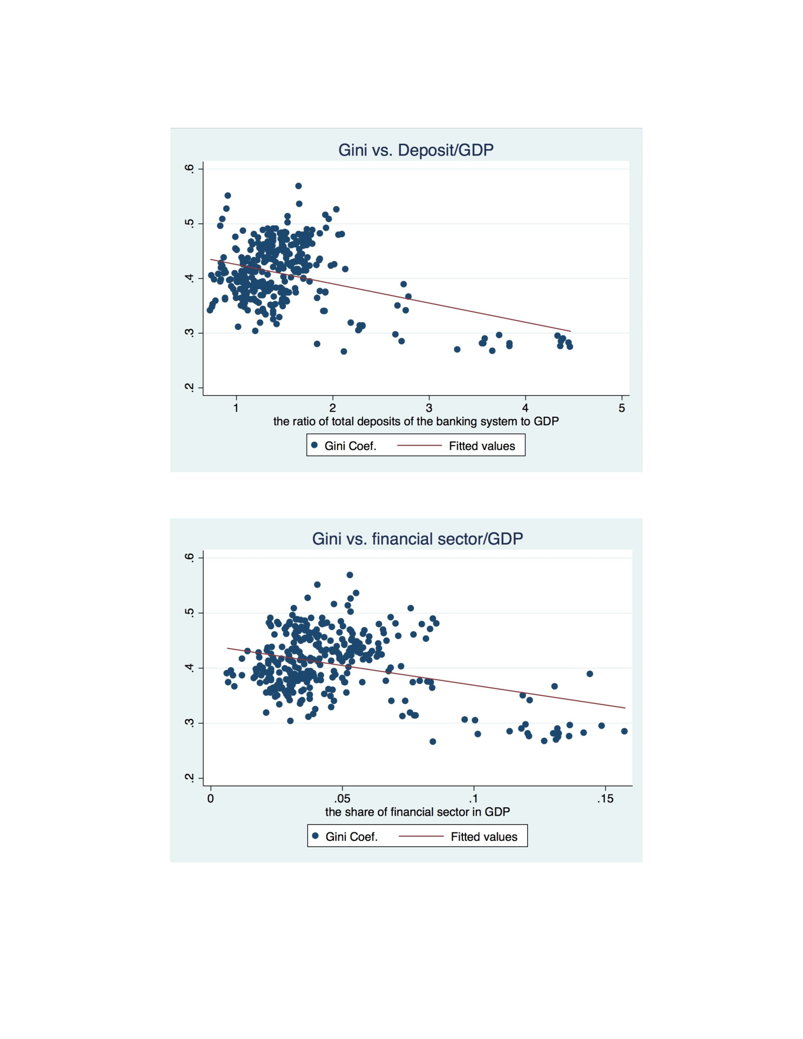
a. Gini vs. The ratio of deposit to provincial GDP

b. Gini vs. The share of financial sector in provincial GDP

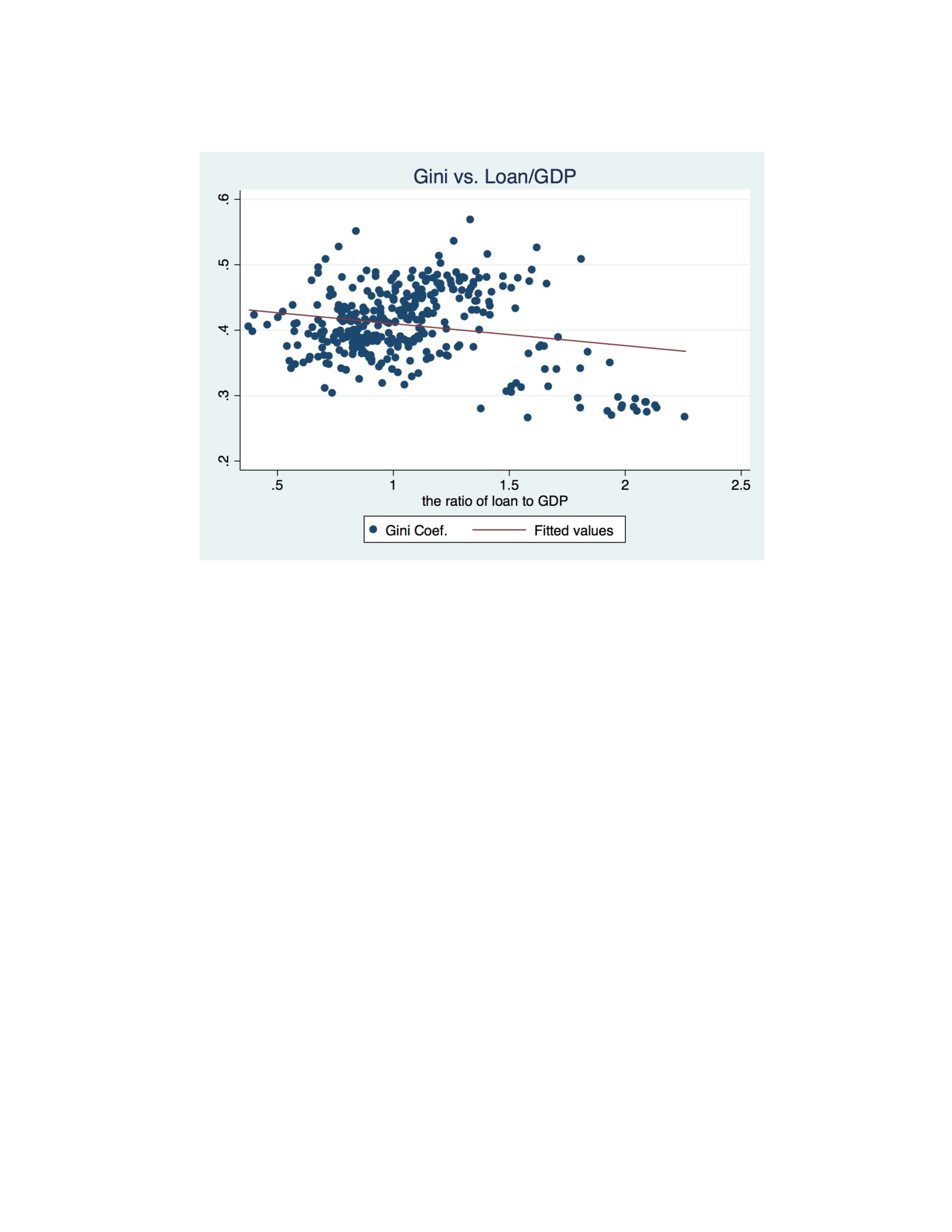
c. Gini vs. The ratio of loan to provincial GDP

Figure 2.A.2: The Scatterplot for Eastern, Central, and Western China

(Y-axis: Gini, X-axis: Each of the measures of financial development)

1. Eastern China

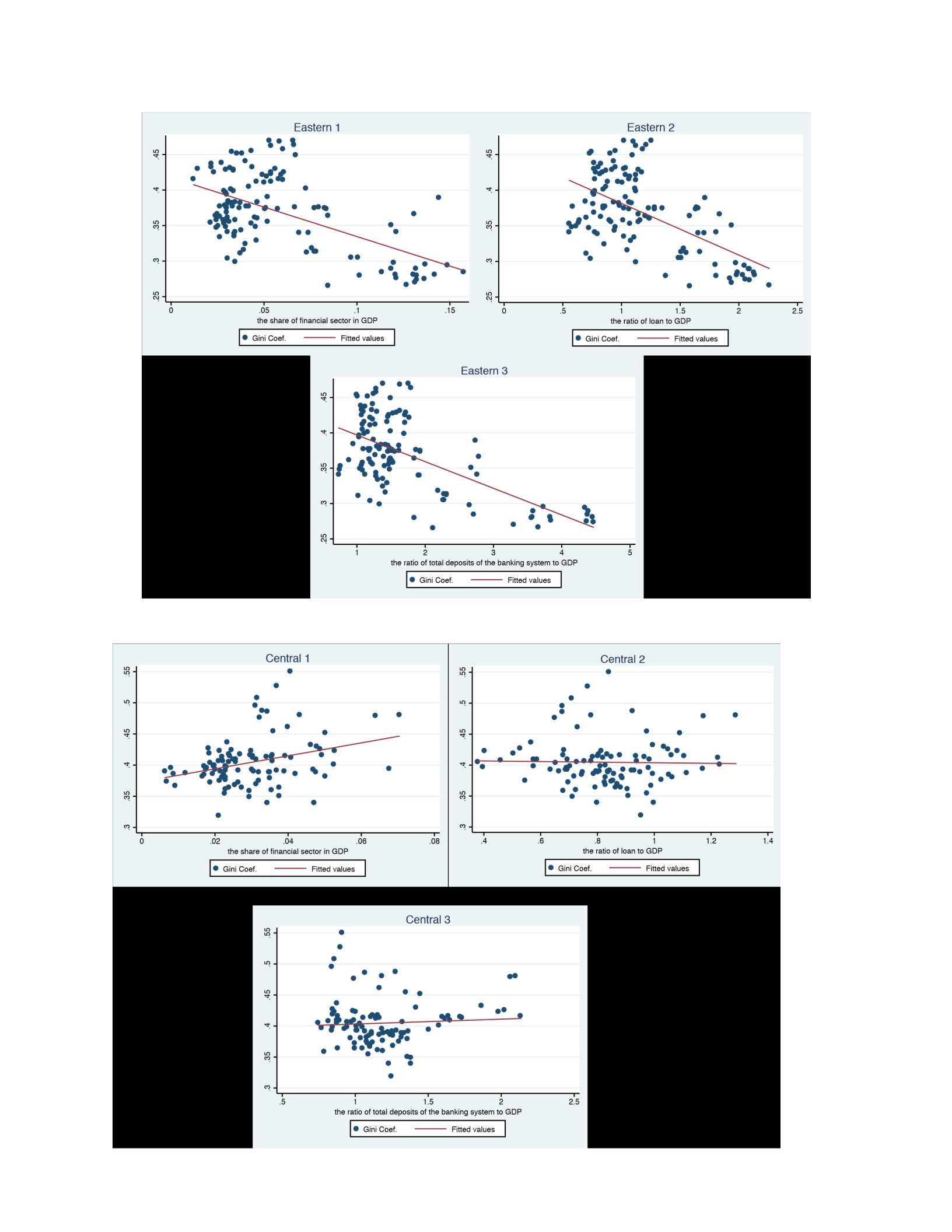
b. Central China

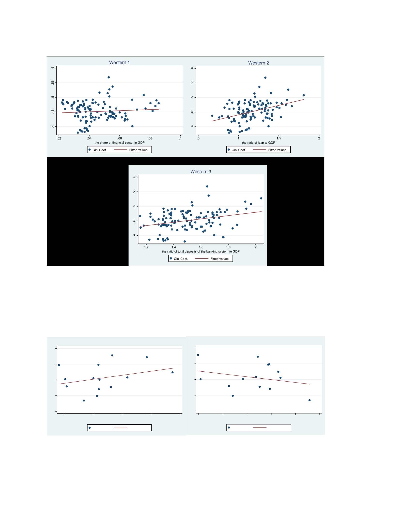
c. Western China

Figure 2.A.3: The Scatterplots for each different province and municipalities

(Y-axis: Gini, X-axis: Each of the measures of financial development) 1.

Eastern China

a. Beijing

.26 .27 .28 .29 .3

12. .13 .14 15. .16

the share of financial sector in GDP

Gini Coef. Fitted values

Beijing 1

.26 .27 .28 .29 .3

1.8 1.9 2 2.1 2.2 2.3

the ratio of loan to GDP

Gini Coef. Fitted values

Beijing 2

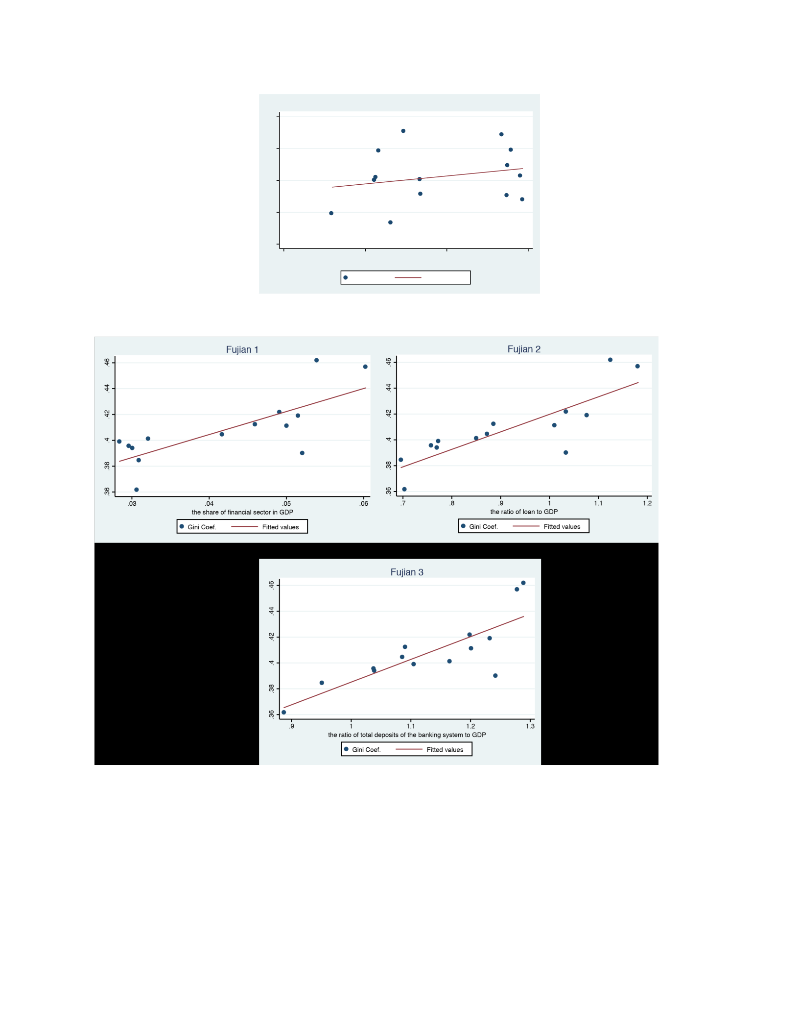
b. Fujian

c. Guangdong

.26 .27 .28 .29 .3

3 3.5 4 4.5

the ratio of total deposits of the banking system to GDP

Gini Coef. Fitted values

Beijing 3

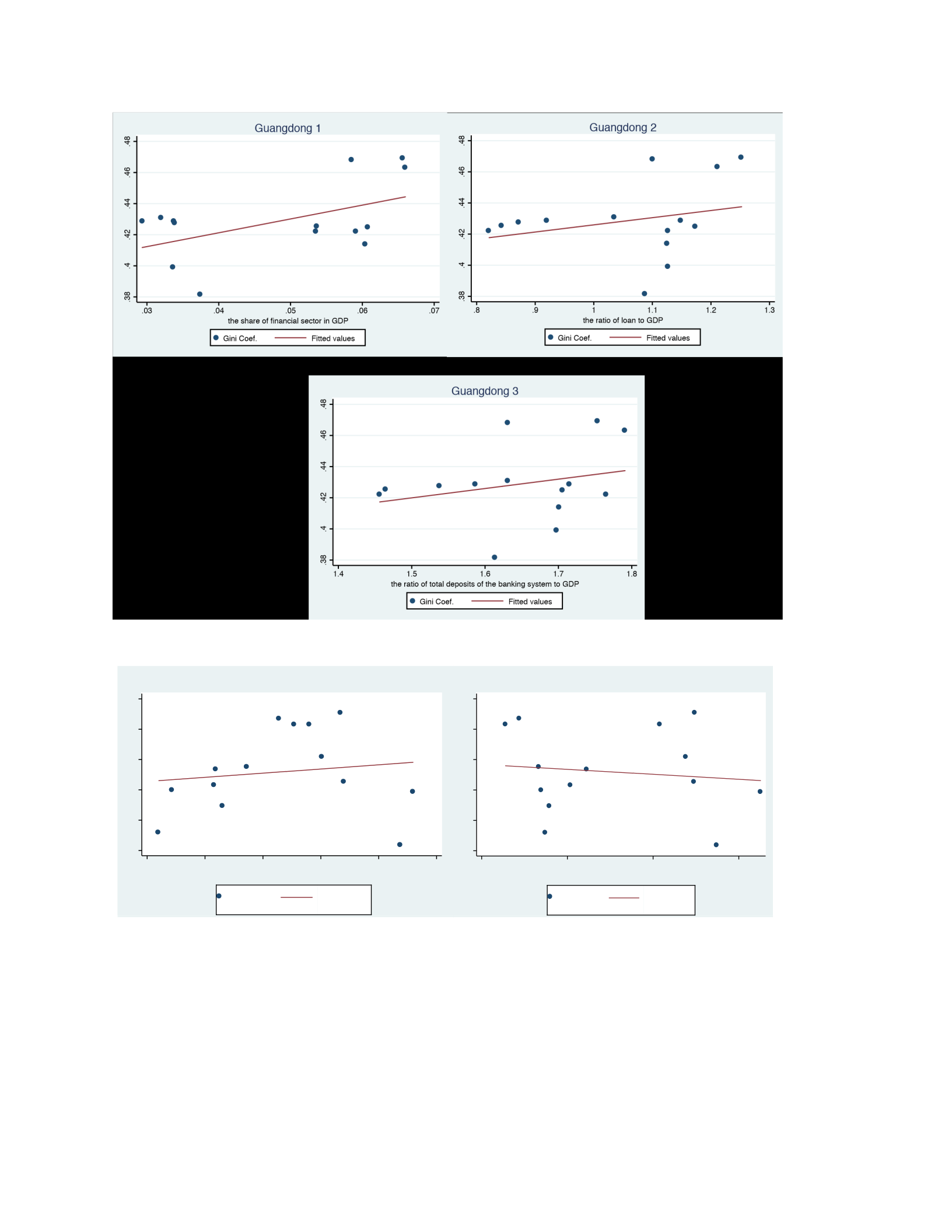
d. Guangxi

Guangxi 1

the share of financial sector in GDP

Gini Coef. Fitted values

Guangxi 2

the ratio of loan to GDP

Gini Coef. Fitted values

.41 .42 .43 .44 .45 .46

.01 .02 .03 .04 .05 .06

.41 .42 .43 .44 .45 .46

.7 .8 .9 1

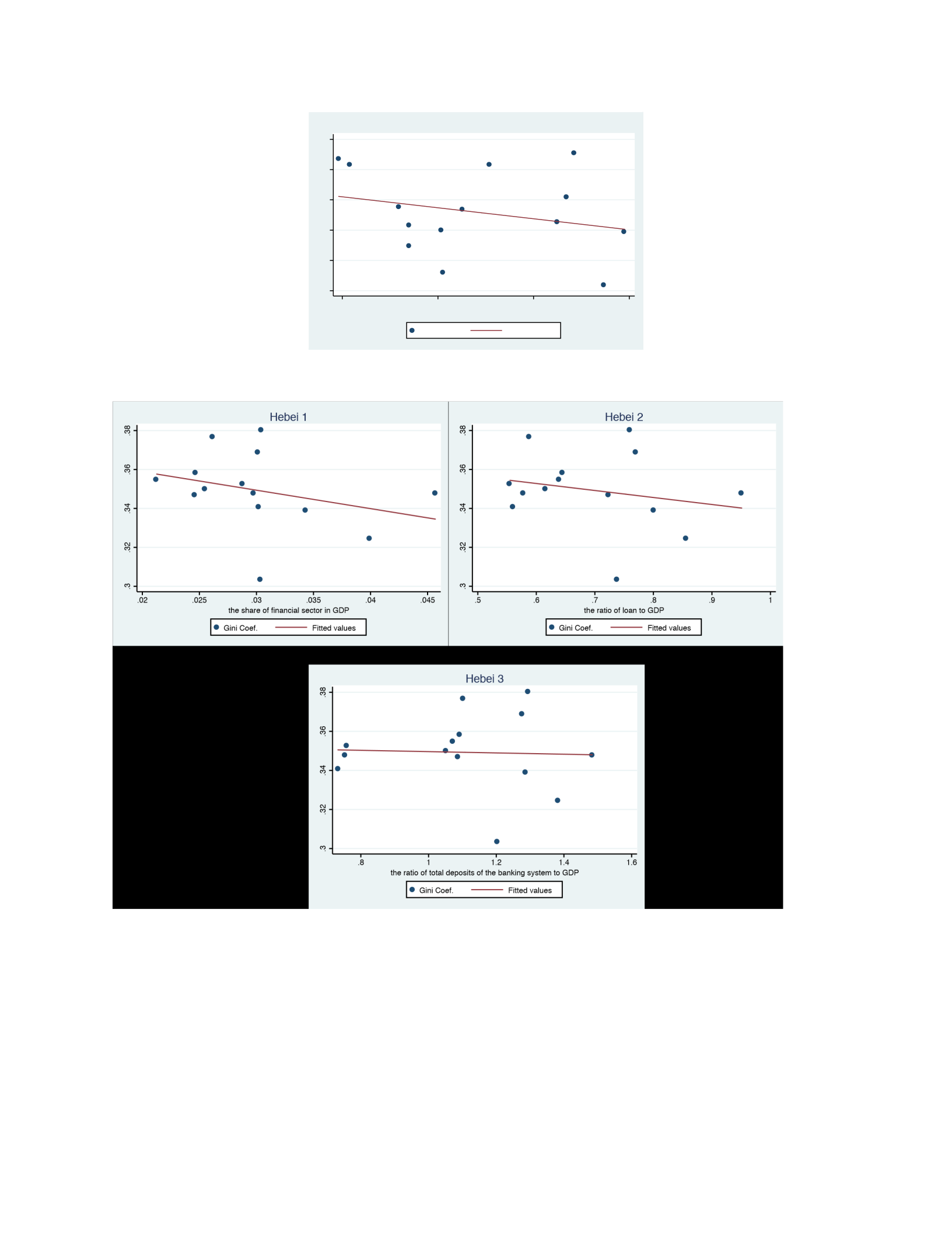
e. Hebei

f. Jiangsu

.41 .42 .43 .44 .45 .46

1 1.1 1.2 1.3

the ratio of total deposits of the banking system to GDP

Gini Coef. Fitted values

Guangxi 3

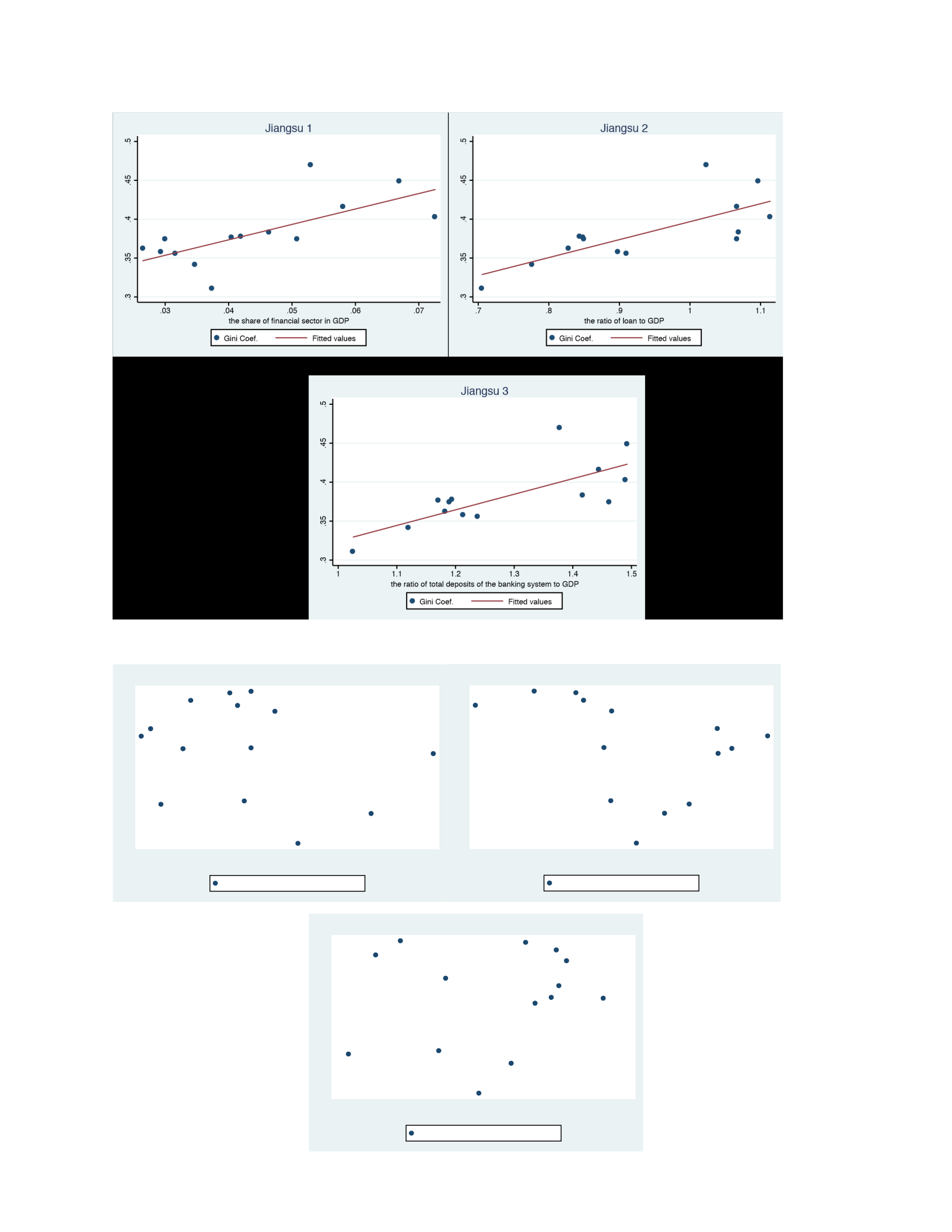
g. Liaoning

.32 .34 .36 .38

.025 .03 .035 .04 .045 .05

the share of financial sector in GDP

Gini Coef. Fitted values

Liaoning 1

.32 .34 .36 .38

.9 1 1.1 1.2

the ratio of loan to GDP

Gini Coef. Fitted values

Liaoning 2

.32 .34 .36 .38

1.3 1.35 1.4 1.45 1.5 1.55

the ratio of total deposits of the banking system to GDP

Gini Coef. Fitted values

Liaoning 3

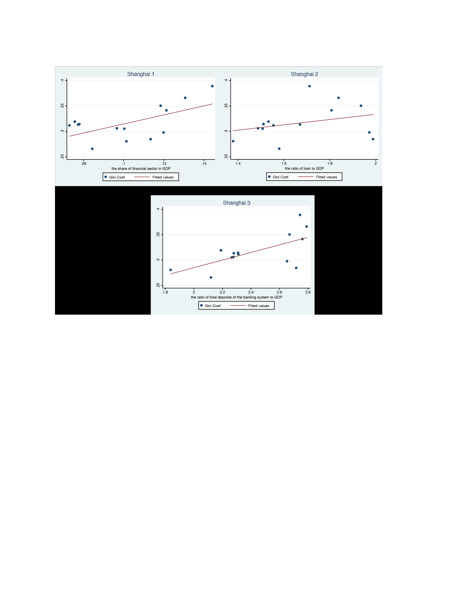
h. Shanghai

i. Zhejiang

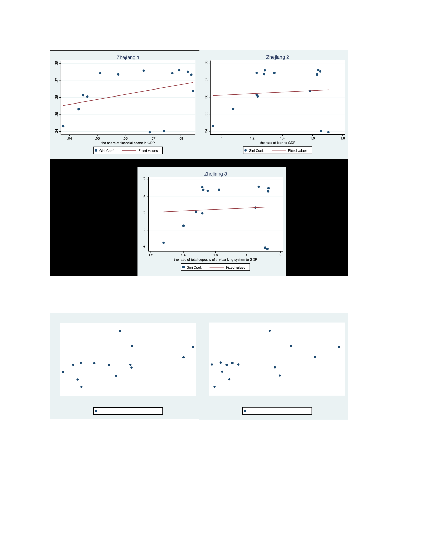
2. Central China

a. Anhui

.35 .4 .45 .5

02. .03 .04 05.

GDPthe share of financial sector in

Gini Coef. aluesFitted v

Anhui 1

.35 .4 .45 .5

.8 .9 1 1.1

the ratio of loan to GDP

Gini Coef. Fitted values

Anhui 2

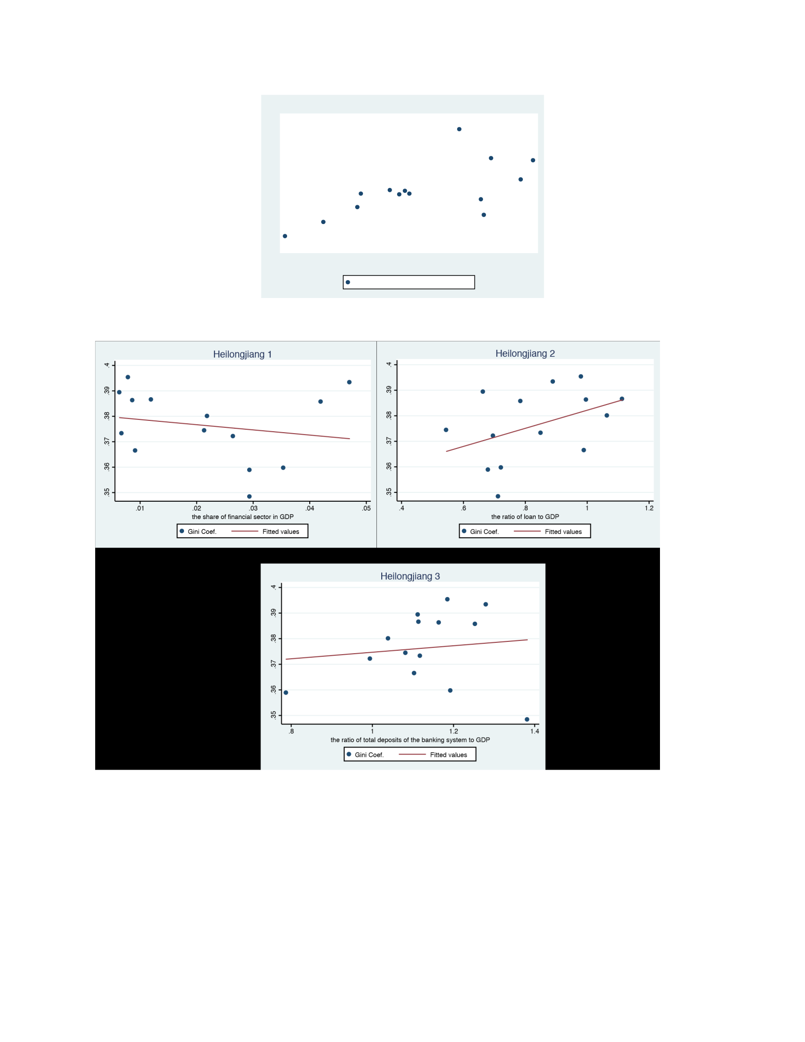
b. Heilongjiang

c. Henan

.35 .4 .45 .5

.9 1 1.1 1.2 1.3 1.4

the ratio of total deposits of the banking system to GDP

Gini Coef. Fitted values

Anhui 3

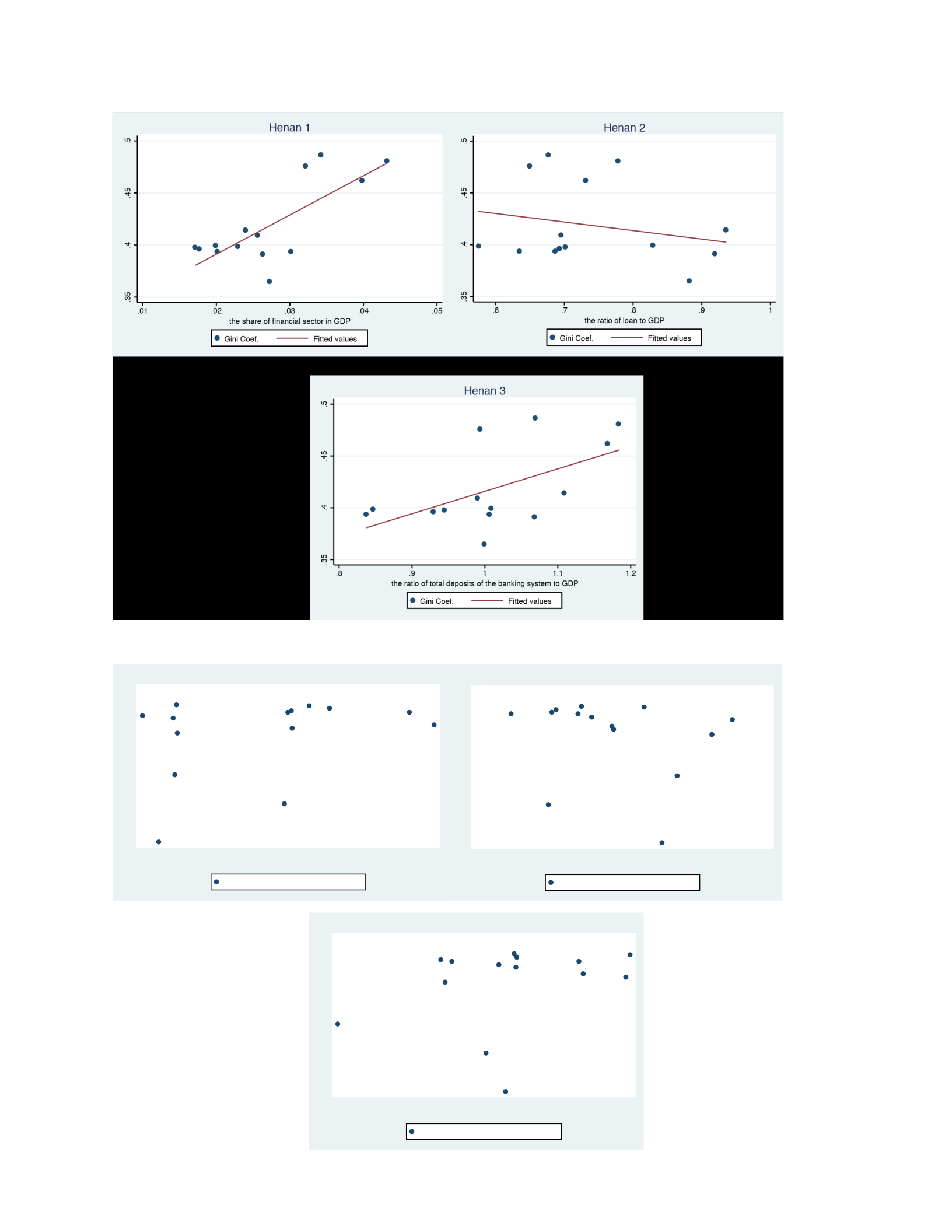
d. Hubei

.32 .34 .36 .38 .4

.02 .03 .04 05.

DPthe share of financial sector in G

Gini Coef. aluesFitted v

Hubei 1

.32 .34 .36 .38 .4

.7 .8 .9 1 1.1

the ratio of loan to GDP

Gini Coef. Fitted values

Hubei 2

.32 .34 .36 .38 .4

1.1 1.15 1.2 1.25 1.3 1.35

the ratio of total deposits of the banking system to GDP

Gini Coef. Fitted values

Hubei 3

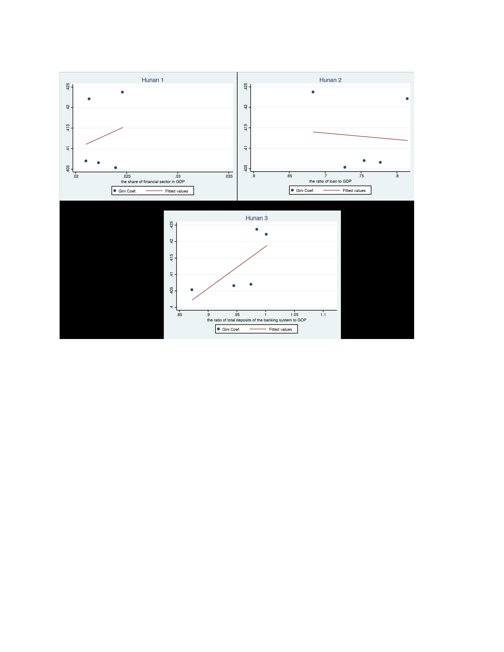
e. Hunan

f. Inner Mongolia

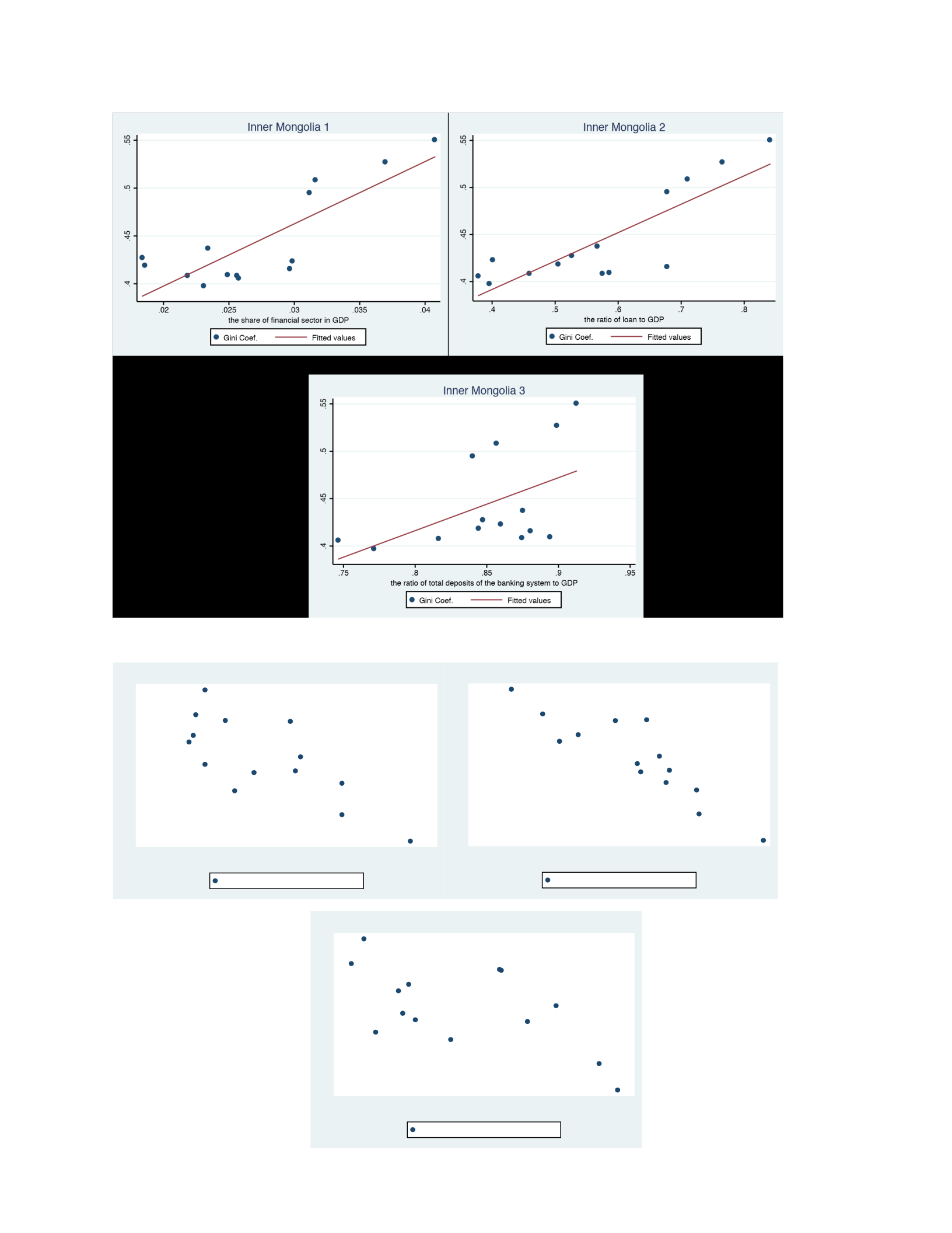
g. Jiangxi

.34 .36 .38 .4

.01 .02 .03 4.0 .05

the share of financial sector in GDP

Gini Coef. Fitted values

Jiangxi 1

.34 .36 .38 .4

.6 .7 .8 .9 1

the ratio of loan to GDP

Gini Coef. Fitted values

Jiangxi 2

.34 .36 .38 .4

1 1.1 1.2 1.3 1.4

the ratio of total deposits of the banking system to GDP

Gini Coef. Fitted values

Jiangxi 3

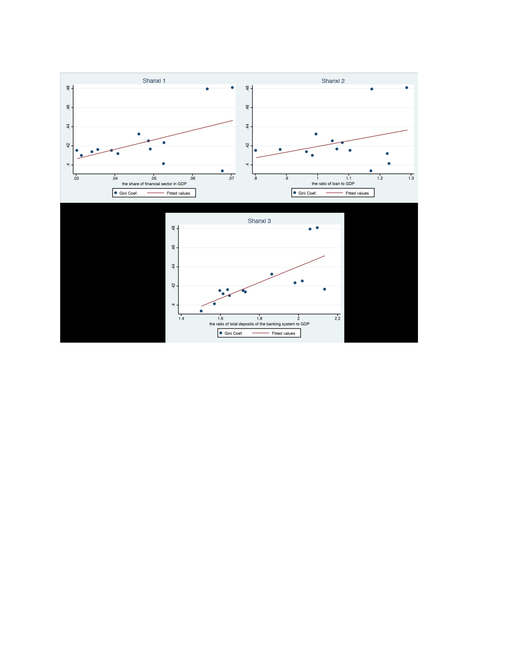
h. Shanxi

3. Western China

a. Chongqing

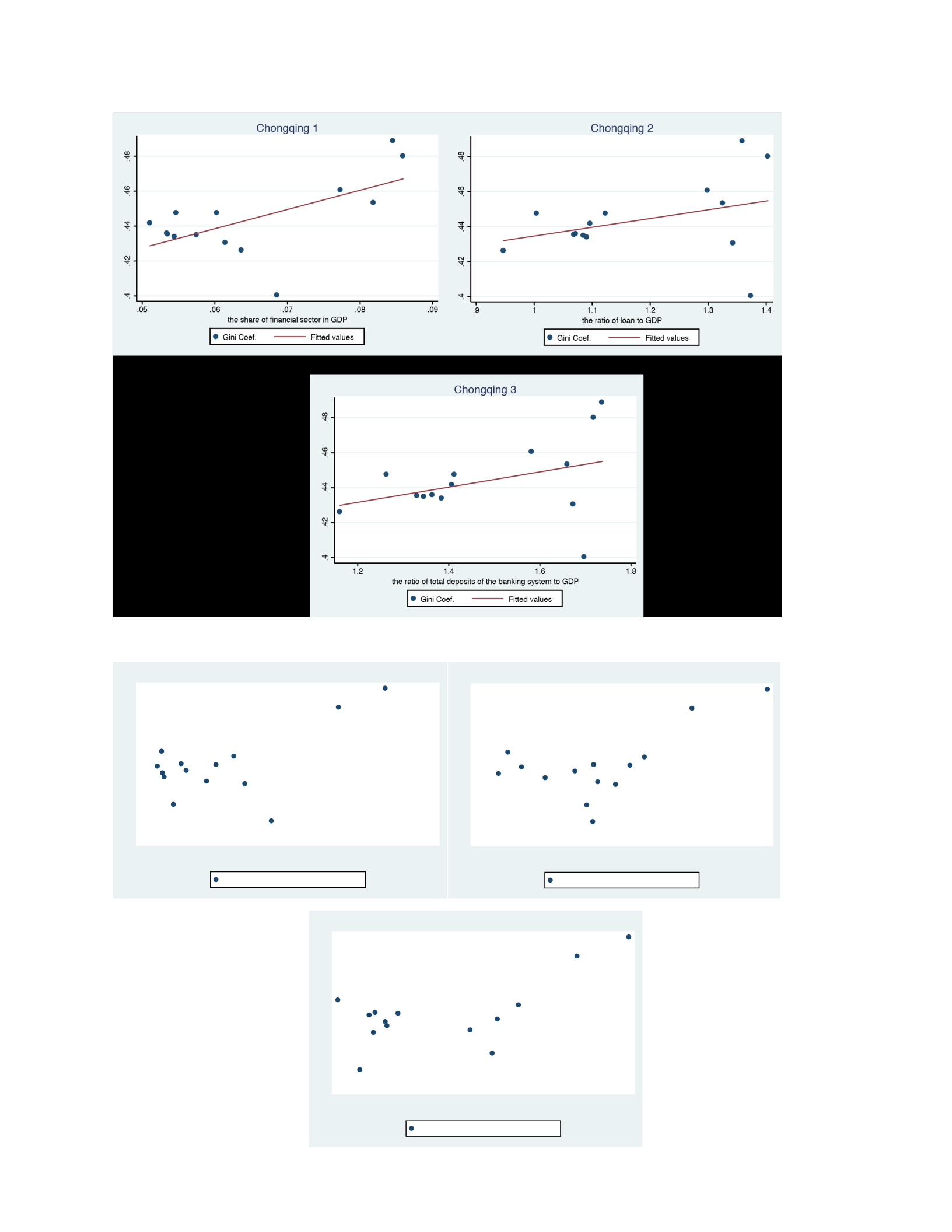
b. Gansu

.44 .46 .48 .5 .52

02. 03. .04 5.0 .06

the share of financial sector in GDP

Gini Coef. Fitted values

Gansu 1

.44 .46 .48 .5 .52

.8 1 1.2 1.4 1.6

the ratio of loan to GDP

Gini Coef. Fitted values

Gansu 2

.44 .46 .48 .5 .52

1.4 1.6 1.8 2

the ratio of total deposits of the banking system to GDP

Gini Coef. Fitted values

Gansu 3

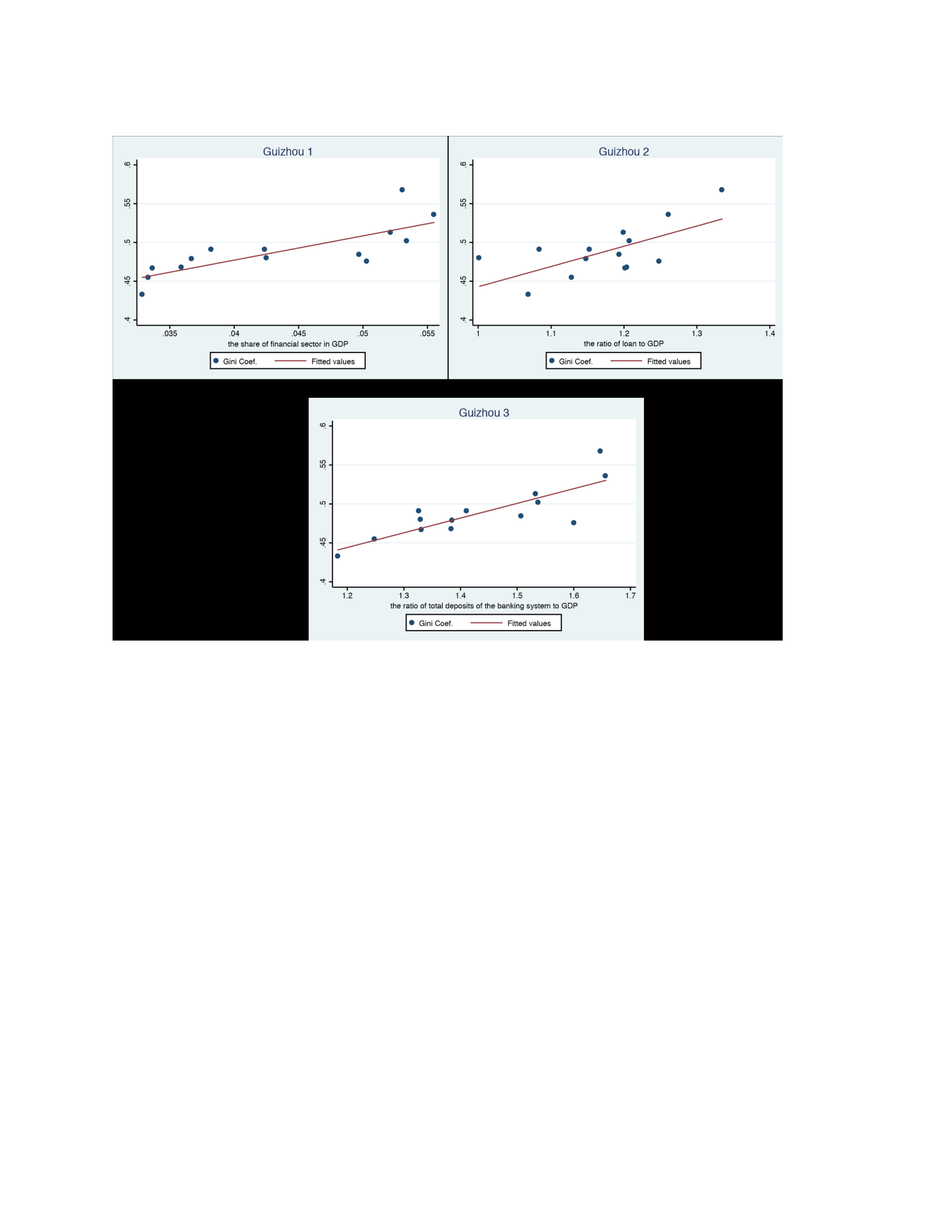
c. Guizhou

d. Ningxia

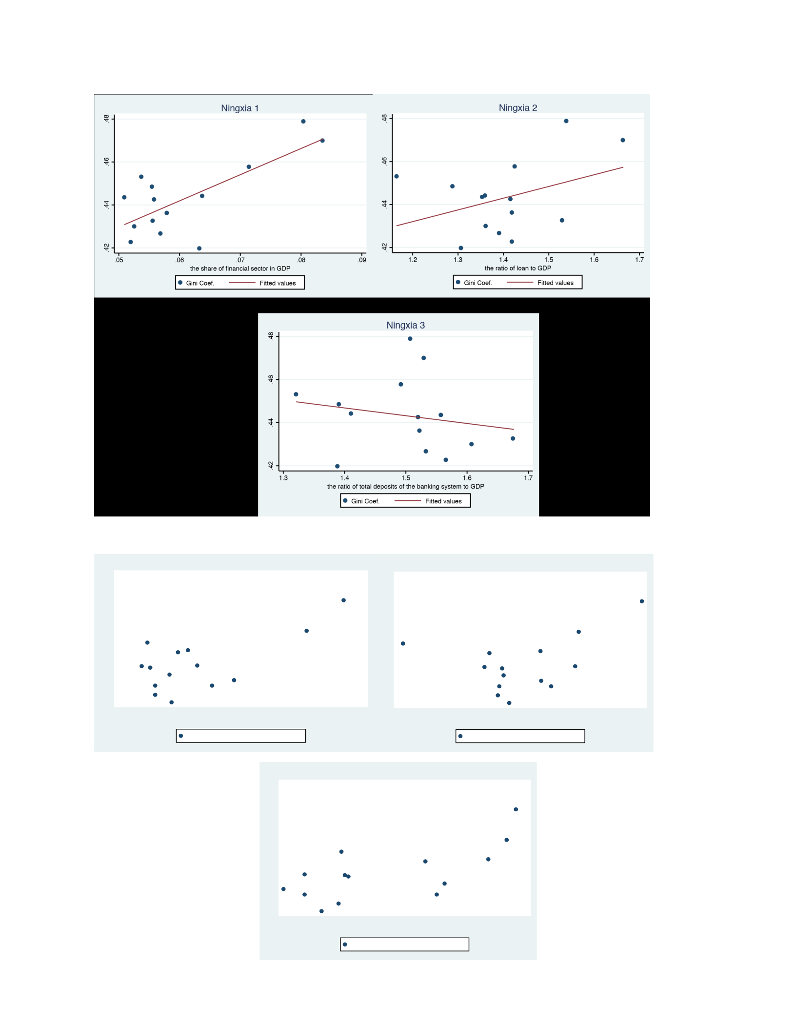
e. Qinghai

.46 .48 .5 .52

.03 .04 .05 .06 .07 .08

the share of financial sector in GDP

Gini Coef. Fitted values

Qinghai 1

.46 .48 .5 .52

1 1.2 1.4 1.6 1.8

the ratio of loan to GDP

Gini Coef. Fitted values

Qinghai 2

.46 .48 .5 .52

1.2 1.4 1.6 1.8 2

the ratio of total deposits of the banking system to GDP

Gini Coef. Fitted values

Qinghai 3

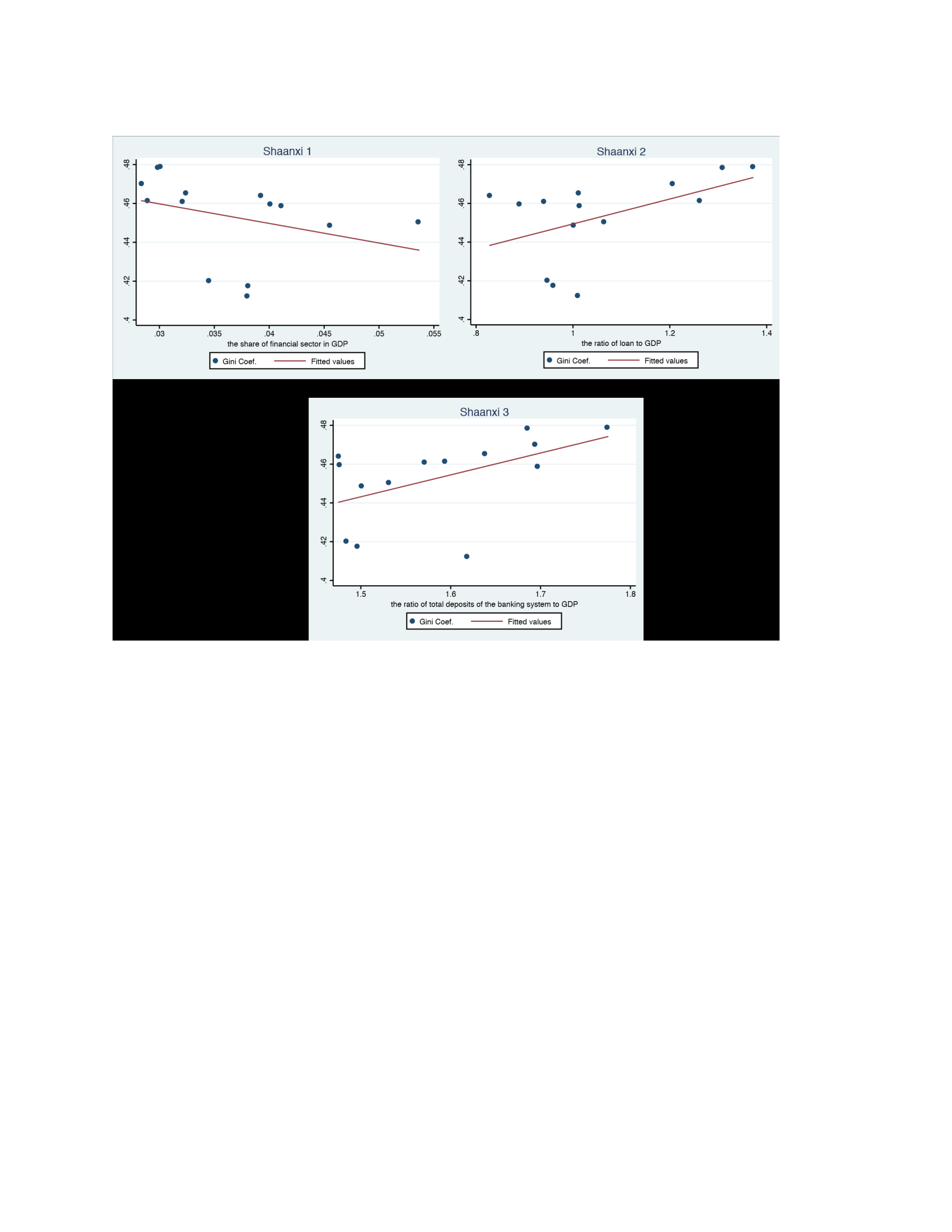
f. Shaanxi

g. Sichuan

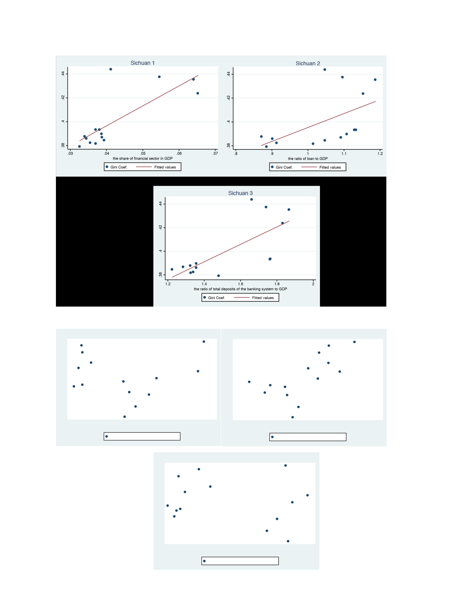
h. Xinjiang

.42 .43 .44 .45 .46

03. .04 05. .06

GDPthe share of financial sector in

Gini Coef. aluesFitted v

Xinjiang 1

.42 .43 .44 .45 .46

.6 .8 1 1.2 1.4

the ratio of loan to GDP

Gini Coef. Fitted values

Xinjiang 2

.42 .43 .44 .45 .46

1.3 1.4 1.5 1.6 1.7

the ratio of total deposits of the banking system to GDP

Gini Coef. Fitted values

Xinjiang 3

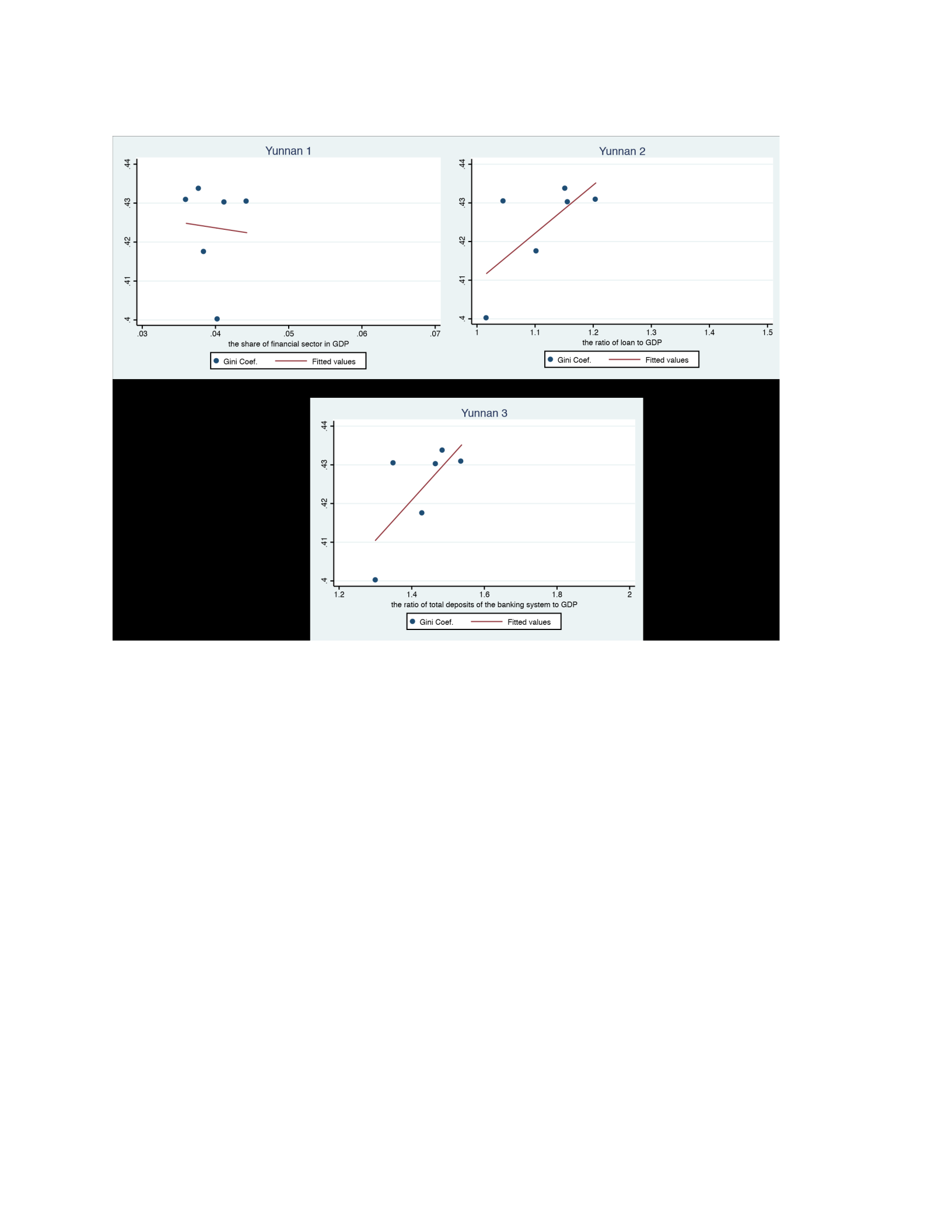
i. Yunnan

3. Financial Development and Income Inequality in China - A Spatial Data Analysis with

Dr. Chu-Ping C. Vijverberg

3.1 Introduction

China has one of the world’s highest levels of income inequality, followed only by South

Africa and Brazil at 0.63 and 0.53, respectively. In the last decade, China’s Gini coefficient

fluctuated between 0.45 and 5.0 (Figure 1), past the warning level to cause social instability or

unhealthy economic development. As is well known, Deng Xiaoping initiated a major policy and

piloted major economic reforms in the late 1970s. One of Deng’s most famous sayings is, “It

does not matter whether a cat is white or black, as long as it catches mice,” The underlying

implication was that both socialism and capitalism are acceptable as long as the people/ society

benefits from them. For these reasons of equality and bettering people’s lives, China opened up

and started expanding economically and socially. After a few decades of high economic growth,

China passed Japan in 2010 to become the second largest economy in the world. Accompanying

this accelerated growth, however, China paid a price in having its income inequality index

ranked as one of the highest in the world, even though economic growth reduced the number of

people under the absolute poverty line. Due to this uneasy rising income inequality and the

concern of its possible negative impact on economic growth, the top priority of China’s twelfth

Five-Year Plan (2011-2015) was to decrease inequality and balance economic development (Fan,

1997; Xinhuanet, 2006). In the increasing concerns on inequality, numerous recent papers

investigate the causes of income inequality. Related research focuses on the following channels

as determinants of inequality: 1) central and local governments’ favorable policies towards

Eastern provinces (Fu, 2004; Kennedy, 2014); 2) human capital accumulation (Cai, Wang and

Du, 2002); 3) foreign direct investment (Wei, Yao, and Liu, 2007); 4) trade openness (Rivas,

2007); 5) decentralization (West and Wong, 1995; Tselios et al., 2012); 6) the multi-mechanism

of socioeconomic, environmental, locational, policy and geographic information system (GIS)

data (Li and Fang, 2014).

Figure 3.1: Recent Trend in China’s Gini coefficient

China’s income inequality has various facets: urban versus rural, coastal versus inland,

within-urban versus within-rural, etc. Most researchers believe that these rising income

disparities have been caused by various institutional and policy factors before and during

economic reforms (Kanbur and Zhang, 2005; Cheng, 2007). In the early years, heavy

industryoriented development strategy, together with the urban-biased monetary and fiscal

policies, generated a sizable income gap between urban and rural areas. Later, due to openness to

international markets, regional development policy, e.g., coastal-biased policy such as providing

favorable tax breaks to coastal provinces to attract foreign direct investment (Kanbur and Zhang,

2005), widened income disparity between coastal and inland provinces. Next and most

importantly, the household registration system (i.e., hukou), where migrant workers have extreme

difficulties changing their officially registered rural residence to urban residence, fortified the

persistent wage gap between urban and rural workers. With the first two contributing factors

being dissolved and “hukou” in the process of being abolished or reformed, China is moving

toward the direction of inequality reduction. However, due to many dimensions of a huge

economy such as China’s, it is unrealistic to consider that the labor market issue is the only

culprit of income inequality in China. More research is needed to understand the dynamics of

0.42

0.43

0.44

0.45

0.46

0.47

0.48

0.49

0.5

2002 2003 2004 2005 2006 2007 2008 2009 2010 2011 2012 2013 2014

China'sGinicoef9icient

income equality, to examine new contributing factors, and to identify ways to reduce income

inequality.

One of dominant motives of income inequality is the effect of financial development (Li,

Squire, & Zou, 1998; Clarke et al., 2003; Beck et al., 2004; Liang, 2006; Wang, 2012; Jauch &

Watzka, 2016). In addition to numerous empirical works on the effect of financial development,

the theoretical connection between financial development and income inequality was mentioned

in Kuznets’s urban possibilities argument (Kuznets, 1955). As the economy develops and society

becomes more urbanized, formerly poor migrants get to choose their education level and

business activities as credits become more accessible in a well-developed financial system. This

decreases income inequality. Theoretical papers connecting income inequality and financial

development predict either a liner or a non-linear relationship. A liner relationship implies that a

well-developed financial system reduces income inequality (Banerjee and Newman, 1993; Galor

and Zeira, 1993) while a non-linear relationship indicates an inverted U-shaped curve – at the

early stage of financial development, due to limited access of credits to a few privileged groups,

income inequality rises, but after a certain stage, financial development reduces income

inequality (Greenwood and Jovanovic, 1990). Thus, while most believe that financial

development decreases income inequality for a mature and advanced economy, financial

development, depending on the stage of economic development, may increase or decrease

income inequality for developing countries. Empirical results of both cross-country and single

country analyses are mixed for both developed and developing countries (Li, Squire, and Zou,

1998; Clarke et al., 2003; Beck et al., 2004; Liang, 2006; Wang, 2012; Jauch and Watzka, 2016).

Since the early 1980s, China’s banking system has been reformed. The four state-owned

specialized banks, known as The Big Four, began to accept deposits and engaged in banking

activities in the 1980s. Even as the Big Four, which dominated more than 60% of the total

financial assets in the Chinese economy, converted to publicly-listed banks and more

domestic/foreign banks joined the system, the Chinese government still has a dominant impact

on banks’ activities in China. According to Bradsher (2013), “…banks in China have been

encouraged by regulators to lend overwhelmingly to state-owned enterprises that appear certain

to repay loans. That has left smaller business and private companies starved for credit.” As of

2012, small and medium-sized private enterprises received about 3% of bank lending even

though their economic activities accounted for at least half of the overall activities. Because

credit accessibility is essential for the implementation of business projects and investment

activities, income generated by these non-privileged groups is obviously affected. Furthermore,

student loans from banks are not common in China. According to Bradsher (2013), although

college entrance is based on the entrance examination, which evaluates students’ academic

ability, and the central government offers grants and need-based loans for students at 4-year

universities, it is still not straightforward for children from poor families to receive financial aid

for their education. In addition, children from poor and rural families tend to perform worse than

rich and urban children on college entrance examinations due to poor training in high school,

particularly in the subject of foreign language such as English. Thus, rich and urban children tend

to have an edge over children from poor and rural families to enter top universities. Bradsher

(2013) stated, “The result that higher education is rapidly losing its role as a social leveler in

China and as a safety valve for talented but poor youths to escape poverty.” The theoretical

concept of decreasing income inequality in a well-developed financial system is an empirical

subject worthy of investigation in China through the linkages of bank credit availability and

education level.

Next, there is a great deal of attention on geographical location to reveal a mechanism of

economic growth or income inequalities (Baker and Grosh, 1994; Hare and West, 1999;

Fingleton, 1999, 2001; Li and Fang, 2014). The majority of these studies investigated

interactions between economic growth and income inequality or between financial development

and income inequality. Since Chinese economic reforms can be summarized by privatization,

industrialization, and urbanization, income disparities among eastern, western, and central

provinces have been widening as shown by real GDP per capita of eastern provinces was 2.24

times higher in 1994. More prominently, real GDP per capita of Shanghai, a municipality in the

east, is 10 times more than the real GDP per capita of Guizhou province in the west. Although it

is theoretically very important to investigate the relationship between financial development,

economic growth, and income inequality, spatial analysis on income disparities is required

mainly because Chinese reform policy has been highly dependent on a friendly environment for

trade, external finance, and a special economic zone in the eastern region. Since each province

has different accessibilities from foreign countries and investments, spatial analysis plays a

pivotal role to reveal the dynamics of income disparities as well as economic growth. According

to Goodchild (2000), recent attention in spatial analysis utilizes insight on spatial issues of

income disparities and improves empirical validity. Recent discoveries facilitating spatial

analysis such as spatial effects, spatial distribution, and the pattern of spatial association shed

light on the association between spatial dependence, spatial heterogeneity, and regional income

inequalities (Rey and Montouri, 1999; Le Gallo and Ertur, 2003), while literature on income

disparities generally overlooks the use of spatial analysis.

Since Chinese economic reforms in the 1970s, provincial growth and development are

extremely uneven so that income inequalities within provinces and inter-provinces have surged

substantially (Zhang and Kanbur, 2005), and regional disparities between the coast and inland are

mainly to blame for income inequalities at the inter-provincial level (Li and Xu, 2008). This

uneven geographical development in China during economic development indicates that an

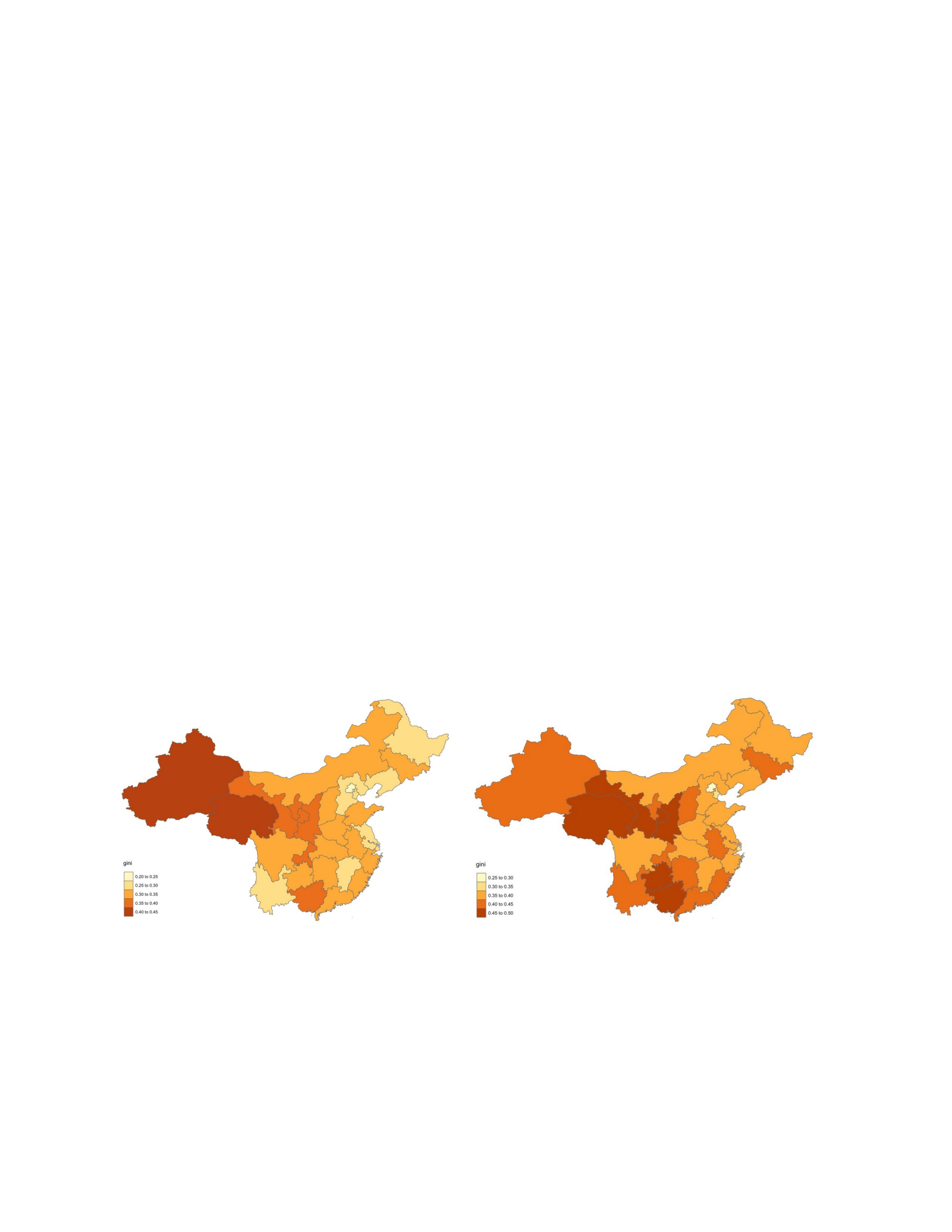
analysis on regional location or space may infer regionally unbalanced development or income

disparities. For this reason, recent empirical research sheds light on the role of spatial effects in

regional inequality in China (Ma, 2006; Hering and Poncet, 2007; De Sousa and Poncet, 2007;

Hering and Poncet, 2010).

Spatial analysis is acknowledged to be a powerful tool (Rey and Montouri, 1999), so

model specification without spatial dependence may cause serious misspecification (Abreu et al.,

2005). As an initial step to this research, Gini coefficient maps in Figure 2 show the spatial

dependence of provincial Gini coefficients, indicating that Chinese provinces are clustered in

1998 and 2014 with similar Gini coefficients. Therefore, to investigate the relationship between

financial development and income inequality in China, the incorporation of spatial dependence in

the model is crucial.

Figure 3.2: Gini Coefficient Maps

Gini map in 1998 Gini map in 2014

In this paper, we evaluate the impact of financial development on income inequality in

China through spatial dependence modeling techniques. In spatial econometrics (Lesage, 1999),

spatial dependence among sample observations is taken into account, where the values of

observations in one group/location may depend on the values in another group/location. This

spatial dependence is not limited to research related to geographical neighbors; it may appear in

the format of economic neighbors, social network structures, etc. Therefore, unlike traditional

time series models that only relate the values of observations over time, spatial dependence

modeling techniques incorporate a peculiar relationship among the observations at a point of

time in the modeling process. There are various ways spatial dependence may occur. In general,

there are different channels that spatial dependence may enter a model: (a) income inequality of a

specific province or municipality is influenced by the inequalities of its surrounding provinces or

municipalities; (b) income inequality of a province is affected by non-observable or

nonmeasurable variable and that effect is captured through spatial dependence in the disturbance

term; for example, central government’s monetary policy or a certain economic reform is

nonmeasureable, but it affects all provinces; (c) a mixture of (a) and (b). In the case of (a) and

(c), the direct and indirect measurement effects are reported.

Our contributions to the literature are the following. First, we use provincial data from

1998 to 2014 to investigate the relationship between provincial financial development and

provincial income inequality in China. As is well known, provincial data of Gini coefficients are

not available for a few provinces and for certain years. To deal with missing data, a GMM

regression is estimated by using available data to obtain predicted values for those missing.

Second, an exploratory spatial analysis is implemented for 29 administrative units in China for

the years of 1998, 2003, 2008, and 2013. The results verify spatial dependence of provincial

income inequalities in China. Third, we use these 29 administrative units in China to fit an

income inequality spatial model by first certifying the necessity of using a spatial model by

implementing Moran’s test on OLS residuals. Next, the LM test is conducted to find a suitable

spatial model. Fourth, due to limited observations in cross-sectional spatial models, we pooled

the data and estimate spatial panel models. The advantage of using spatial panel model is not

limited to just observing more data points. Due to sequential observations for 18 years, the panel

model may capture the interactions between financial development and provincial income

inequality and provide some dynamics in a relationship that the cross-sectional model could not

produce. Thus, our analysis provides a special angle to look into China’s income inequality

issue.

This paper is organized as follows. Section 2 reviews previous literature on spatial

analysis of interprovincial inequality. In Section 3, we briefly present methods of spatial data

analysis and the data. In the fourth section, applying a provincial level dataset of China over the

period from 1998 to 2014, we calculate global and local Moran’s I, which are spatial

autocorrelation statistics, draw the Moran scatterplot, and estimate spatial panel models. Lastly,

Section 5 reviews the main findings for spatial data analysis on interprovincial inequalities.

3.2 Literature Review

In an effort to introduce spatial impacts into inequality analysis, Rey (2001) calculated

the Theil index and Moran’s I statistics with U.S. state income data from 1929-2000. Although

he found a positive relationship between these two measures in various spatial partitionings –

Census regions, Census division, and BEA (Bureau of Economic Analysis) – and arrangements,

policy implications are difficult to derive from this discovery.

Le Gallo and Ertur (2001) believed that, due to spatial interactions between regions,

geographical location is relevant in examining regional economic performances. They evaluated

the relationship between the spatial dependence and the distribution of regional GDP per capita

in Europe using 138 regions for 11 European counties between 1980 and 1995. By observing

global and local spatial autocorrelations, they portrayed the way economic activities are located

in the EU. The authors conformed a strong association between spatial dependence and the

distribution of regional per capita GDP in Europe throughout the whole sample period between

1980 and 1995. Additionally, by identifying clusters of high and low per capita GDP during the

sample period, they illustrated a persistence in the geographical disparities between European

regions. Kanbur and Zhang (2005) analyzed regional inequality in China with a long-run time

series dataset. To capture the key economic policies during economic transition, three policy

indicators were created: (1) an indicator of the bias against agriculture and China’s comparative

advantage to investigate how a lack of government support in the agricultural industry and the

surge in heavy industry led to an increase in inequality between urban and rural; (2) an indicator

of the degree of openness to capture how policy of international economic integration, a driving

force of economic development in China, affects regional inequality; (3) an indicator of

decentralization to analyze how local government’s fiscal budget controlling power granted by

the central government during economic reform influences income disparities. The empirical

findings suggested that heavy-industry development strategy was the most dominant cause of

urban and rural inequality in China and that policy of international economic integration and

fiscal decentralization resulted in the surge of inequality between inland and coastal provinces

during the reform period of the 1980s and 1990s.

As for geographical studies on Chinese regional inequalities, Wei and Ye (2009)

investigated regional inequality in Zhejiang, a province at the forefront of Chinese economic

growth, using an extensive county-level dataset and adopting exploratory spatial data analysis

techniques of global and local Moran’s I, Space-Time Analysis of Regional System, and

geographically weighted regression. They found that regional inequality in Zhejiang province of

China exhibited strong spatial autocorrelation, while the level of regional inequality in Zhejiang

increased during the Chinese economic transition period and a partition between interior and

coastal Zhejiang formed. Similarly, Wei, Yu, and Chen (2011) investigated regional inequality in

Jiangsu province of China using a spatial Markov chain analysis, Moran’s I, and geographically

weighed regression analysis. They discovered a general increasing trend of regional inequality

and revealed a surge in regional inequality that resulted from rapid development in southern

Jiangsu. They also mentioned that northern Jiangsu was confronted with developmental

difficulties due to strong geographical barriers. Findings from the spatial Markov chain analysis

suggested that the level of development for geographically neighboring counties strongly affects

a county’s level of development. For example, if a county with a low level of development is

neighboring a county with a relatively high level of development, the low developmental county

has a relatively higher developmental level than other low developmental counties neighboring

relatively poor counties. The empirical findings from the geographically weighted regression

analysis revealed that a county’s developmental dynamics are strongly correlated with local

characteristics.

Recently, Li and Fang (2014) investigated the multi-mechanism of regional inequality

from 1992 to 2010 with spatial panel data models. They categorized the explanatory variables

into socioeconomic, environmental, locational, and policy factors and constructed indicators to

represent each of the categorized variables. The authors found that a non-stationary dynamic

structure is captured in Chinese regional inequality. In addition, the spatial panel data analysis

demonstrated that each socioeconomic, environmental, locational, and policy factor was

statistically significant while their impact on regional inequality gradually disappeared. More

significantly, they illustrated that spatial panel models are superior to OLS techniques and,

therefore, concluded that spatial data analysis is more suitable in revealing regional inequality

and development. Unlike Li and Fang (2014), our paper uses provincial data from 1998 to 2014

to analyze the association between financial development provincial income disparities in China

after missing Gini coefficients are estimated by using available provincial data. This advantage of

panel provincial data enables us to see some dynamics in a relationship.

3.3 Methodology and Data

Anselin (2005) argued that before the spatial regression model is estimated, exploratory

spatial data analysis should be applied as a preliminary step. In order to test spatial dependence,

the spatial autocorrelation is calculated using Moran’s I, which is a weighted correlation

coefficient, and can be visualized using the Moran scatterplot (Anselin, 1988). Moran’s I ranges

between -1 and +1, where a positive I indicates positive spatial autocorrelation, which occurs

when similar values for the random variable are clustered together in space. A zero value of

Moran’s I presents a random spatial pattern. For example, if a value of Moran’ I is close to 1,

there is strong and positive spatial autocorrelation. On the other hand, if a value of Moran’s I is

close to -1, there is a strong but negative spatial autocorrelation. Moran’s I is calculated as:

N ∑i ∑ j wij (yi −y) (yj −y)

I2 (1) i j ∑i (yi

−y)

where wij is an element of a binary spatial weights matrix W such that wij = 1 if states i and j

share a border and zero otherwise. yi is per capita income in province i and y is the average per

capita income for the 29 administrative units.

Next, the Moran scatterplot visualizes the spatial association for exploratory analysis

(Anselin, 1996) since it presents how similar an observed province is to its geographically

neighboring province. The horizontal X axis, which is called the response axis on the Moran

scatterplot, indicates the values of observations, while the vertical Y axis specifies the weighted

average of the neighboring observations on the response X axis. In the Moran scatterplot, there

are four quadrants of the scatterplot defined by the horizontal line y=0 and the vertical line x=0,

indicating different spatial associations, respectively. Quadrant 1 in the top right (or high-high)

presents values with positive spatial association higher than the sample mean, while Quadrant 3

in the bottom left (or low-low) presents values with positive spatial association lower than the

sample mean. In the same way, Quadrant 2 in the top left (or low-high) and Quadrant 4 in the

bottom right (or high-low) correspond to negative spatial association, meaning each observation

exhibits dissimilarity to its geographically neighboring observations.

However, the global Moran test discussed above does not enable us to identify the

regional structure of spatial autocorrelation because global spatial autocorrelation analysis

produces the test statistic with the homogeneity assumption that the same patterns occur over the

whole geographic area, while the local Moran test assumes that different patterns or processes

may occur in different locations of the overall area. Since the global Moran test statistic is

calculated from the local relationships between the observed values at a spatial entity and its

neighboring observations, Anselin (1995) suggested Local Indicators of Spatial Association

(LISA), which breaks the global measures into two different components and construct localized

tests to search for clusters and hotspots. The local Moran test statistic for a unit i is

Ii = zi ∑wijzj j (2)

zi = yi −y (3)

SDy

where zi is the original variable yi in standardized form, SDy is the standard deviation of y, wij is

the spatial weight, and the summation is referred to summing the neighboring values from each

row i of the spatial weights matrix. A positive LISA value indicates that a feature has

geographically neighboring features with similarly high or low attribute values (a cluster) while a

negative LISA value implies that a feature has neighboring features with dissimilar values (an

outlier). Also, the significance map shows those regions with different significant levels of LISA

(Anselin, 1995).

The goal of this paper is to investigate spatial interactions of financial development and

provincial income inequality in China between 1998 and 2014. A further step delves into the

spatial determination of income inequality, where spatial models such as a spatial lag model and

spatial error models are applied to allow for the spatial dependence of income inequality. First, as

reviewed by Anselin (1988) and Anselin and Bera (1998), in the spatial lag model, spatial

dependence is expressed by spatial autocorrelation, which explains how a province’s Gini

coefficient can be influenced by the Gini coefficients in surrounding provinces. The spatial lag

regression model can be expressed as:

y=ρW1y+Xβ+u (4)

where y is a n times 1 vector of observations, W is a n times n spatial weight matrix, X is a n by k

matrix of k explanatory variable, β is a k times 1 vector of coefficients, ρ is the spatial lag

dependence or spatial autoregressive coefficient that is supposed to be between -1 and +1,

measuring how neighboring observations affect the dependent variable, and u is a n times 1

vector of uncorrelated error terms. More exactly, its lower bond is sometimes stated to be -1 but

this is actually quite in doubt. The model is likely unstable if it is close to -1. Rather, it should be

greater than the smallest eigenvalue of W (i.e., the largest negative eigenvalue). The spatial

weight matrix (W) consists of Wij, which measures the relative location of all point i and j. In this

study, spatial neighbors are based on contiguity (or adjacency): 1) Wij is equal to 1 if provinces

share their border; 2) Wij is equal to 0 if provinces do not share their border.

Second, the spatial error model is estimated by maximum likelihood with a spatial error

term. In this case, a shock in surrounding provinces spills over through the error term. It begins

with equation (5) having spatial errors of equation (6).

y=Xβ+u (5) u=λWu+e (6)

where u is the vector of error terms, spatially correlated by means of the weights matrix (W), 𝜆 is

the spatial error coefficient, and e is a vector of uncorrelated error terms. By substituting

equation (6) into (5), the spatial error model is

y= Xβ+(I −λw)−1e (7)

Equation (7) illustrates the spatial correlation in its error term: whereas e is uncorrelated,

(I −λW)−1e is correlated whenever λ≠0.

Lastly, we consider the spatial lag and error model, which starts from

y=ρW1y+Xβ+u (8) u=λW2u+e (9)

By substituting equation (9) into (8), the spatial lag and error model is

y=ρW1y+ Xβ+(I −λW2)−1e (10)

where u is the vector of error terms, spatially weighed with the weight matrix (W2), ρ is the

spatial lag dependence, measuring the average influence on observations by their neighboring

observations, λ is the spatial error coefficient, and e is a vector of uncorrelated error terms.

In the spatial econometric literature, the three models are special cases of the SARAR (p,

q) model where p denotes the number of spatial lags of y and q denotes the number of spatial

lags in the error. Thus, the spatial lag model in equation (4) is a SARAR (1,0) model; equations

(5)-(6) are the SARAR (0,1) model, and equation (8)-(9) are the SARAR (1,1) model. To

investigate the impact of spatial dependence and spatial scale on interprovincial inequalities, as

shown in Table 3.1 and Figure 1, we use the definition of formal administrative units in China

provided by the Seventh Five-Year Plan. It is frequently used for analysis on regional inequality

in China (Fan, 1995a; Lee, 2000; Wei, 2000). The Western region includes nine provinces and

one municipality, the Central region includes nine provinces, and the Eastern region includes 10

provinces and two municipalities. Since Tibet is frequently omitted from research on regional

income disparities (Zhang, 2003; Chen, 2006), we also exclude Tibet from the spatial analysis in

this paper. After 2006, the Central Chinese government added a new region, the Northeastern

region (Heilongjiang, Jilin, and Liaoning provinces) and announced the Four Region Division

policy (Central, Eastern, Northeastern, and Western regions) in the Eleventh Five-Year Plan.

However, our analysis is based on the Eastern, Central, and Western divisions.

Table 3.1: Administrative Regions in China

Region Provinces and municipalities

Eastern Fujian, Guangdong, Guangxi, Hainan, Hebei, Jiangsu,

Liaoning, Shandong, Tianjin, and Zhejiang and two

municipalities Beijing and Shanghai

Central Anhui, Henan, Heilongjiang, Hubei, Hunan, inner Mongolia,

Jiangxi, Jilin, Shanxi

Western Gansu, Guizhou, Ningxia, Qinghai, Shaanxi, Sichuan, Tibet,

Xinjiang, Yunnan, Chongqing

Figure 3.3: Provincial Level Units in China

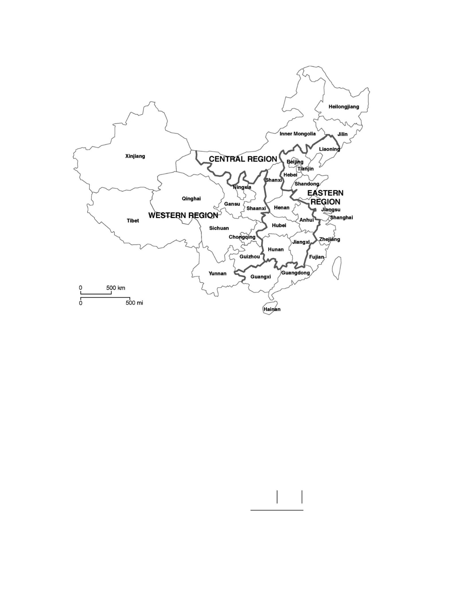
Source: Seventh Five-Year Plan for National Economic and Social Development of the People’s Republic of China

The provincial GDP and Gini coefficient for spatial analysis are from a cross-sectional dataset

of 29 Chinese provinces and municipalities over the period between 1998 and 2014 provided by

the Chinese Statistical Yearbook of each province and the Almanac of China’s

Finance and Banking published by the National Bureau of Statistics of China. For this paper,

Gini coefficients are used to account for provincial inequalities mainly because only Gini

coefficients are promptly reported by China’s National Bureau of Statistics (NBS). The Gini

coefficient is presented as:

∑n ∑n xi −xj

G= i=1 nj=1 n (11)

2∑∑xj

i=1j=1

where xi is the wealth or income of person i, and n is the number of people.

To deal with the missing Gini values, we use the following X matrix for prediction (y

variables are Gini coefficients in neighboring provinces).

X = (lgdp_ca, open, edu, f_gdp) (12)

The vector X contains the set of control variables: (1) the logarithm of provincial GDP per capita

(lgdp_ca); (2) the degree of provincial economic opening to foreign countries (open) as

measured by the ratio of the sum of exports and imports to provincial GDP; (3) educational

attainment (edu), the share of the population with more than secondary schooling as a proxy for

education development; (4) the ratio of the value-added of financial intermediation to provincial

GDP (f_gdp), where the value-added of financial intermediation is the final result of

marketpriced value-added of the products produced by all residents engaged in finance.

Previous papers utilized global Moran’s I, local Moran’s I, and Moran scatterplots to investigate

spatial dependence of income inequality or economic growth. Researchers have rarely used

spatial models to analyze China’s provincial income inequality. One of the primary reasons is

missing Gini in some provinces and municipalities, i.e., Hunan, Jilin, Shandong, Tianjin, and

Yunnan. For the spatial model analysis, the weight matrix is an essential element of the model.

However, if several provinces have missing values, the spatial model cannot provide an

adequate analysis through the weight matrix. Thus, to overcome missing data for a specific

province or municipality, we estimate a GMM regression model for its neighboring provinces

using observed Gini data to obtain the predicted Gini for the provinces (or municipalities) with

the missing Gini.18

giniit =β1giniit−1 +β2Fit' +β3Xi't +µi +λt +εit (13)

where Gini is each provincial Gini coefficient, µi is a provincial random effect, λt is a time fixed

effect, and εit is an error term.

One issue in using equation (13) to obtain the predicted Gini coefficients for missing

values is the missing provincial random effect. In the case of Hunan, for example, to construct a

better prediction, the average of the values of εit in neighboring provinces (i.e., Chongqing,

Guangdong, Guangxi, Guizhou, Hubei, and Jiangxi) is computed and then added to the estimated

Gini coefficients of Hunan. All other missing Gini coefficients are calculated in the same way.

3.4 Empirical results

We do an Exploratory Spatial Data Analysis and estimate a spatial econometrics model to

investigate the spatial relationship between financial development and income inequality. Since

we use the estimated Gini coefficients from the GMM model above, the data sample for this

spatial analysis includes 29 administrative units (i.e., 21 provinces, 4 municipalities, and 4

autonomous regions) in China over the period between 1998 and 2014. To illustrate the overall

spatial trend over this, we choose 1998, 2003, 2008, and 2013 ─ the beginning and the end of the

data sample and those five years apart ─ as representative cases.

3.4.1 Global Moran Statistics

Table 3.2 reports the Moran’s I statistics for Gini coefficient between 1998 and 2014 for

the 29 Chinese administrative units, indicating a global significant trend to spatial

autocorrelation. For all sample years, the null hypothesis of spatial randomization is rejected

because Moran’s I statistics is significant at the 1% significance level. This tells us that provinces

having relatively large Gini coefficient are close to other provinces having relatively large Gini

coefficients and provinces with low Gini coefficients are close to provinces with low Gini

coefficients. Another finding is that Moran’s I statistics increased from 0.456 to 0.629 between

1998 and 2001 and thereafter (after WTO entry) decreased to 0.315, indicating that, over the

years, spatial dependence increases and then decreases.

Table 3.2: Moran’ I Statistics for Gini coefficient

Year Moran’ I Standard Deviation

1998 0.456*** 0.136

1999 0.626*** 0.134

2000 0.618*** 0.134

2001 0.667*** 0.134

2002 0.629*** 0.134

2003 0.626*** 0.134

2004 0.517*** 0.138

2005 0.584*** 0.134

2006 0.584*** 0.134

2007 0.596*** 0.135

2008 0.526*** 0.135

2009 0.511*** 0.133

2010 0.474*** 0.133

2011 0.374*** 0.137

2012 0.342*** 0.136

2013 0.309*** 0.137

2014 0.315*** 0.136

Note: ***, **, and * indicates significance at the 1%, 5%, and 10% level, respectively.

3.4.2 Local Indicator of Spatial Autocorrelation (LISA)

LISA is used to identify patterns of significant spatial clustering of similar or dissimilar

values among the provinces. As presented in Table 3.3, in 1998, most Western provinces (Gansu,

Ningxia, Qinghai, Shaanxi, and Xinjiang) have a significant positive value of local Moran’s I,

which suggests there is a “cluster” of high values of Gini analyzed with reference to the average

of all provinces in that year. Second, some Eastern provinces or municipalities such as Beijing,

Jiangsu, Shanghai, and Tianjin, which were the most urbanized municipalities and provinces in

China in 1998, have a significant positive value of local Moran’s I, pointing to a tendency

towards clustering of high values, while Central provinces have no significant value of local

Moran’s I. In 2013, Central provinces do not show any significant value of local Moran’s I, but

Eastern provinces or municipalities (Beijing, Hebei, Tianjin, and Zhejiang) do, specifying a

highvalue cluster. In addition, Western provinces (Gansu, Ningxia, and Qinghai) show a

tendency towards a clustering of high values.

Table 3.3: Local Indicators of Spatial Association: Gini coefficient

Province or

Municipalities

Region 1998 2003 2008 2013

Anhui Central -0.004 -0.118 -0.078 -0.054

Zhejiang Eastern -0.031 0.541* 0.346 0.229*

Jiangxi Central -0.178 0.014 -0.001 0.094

Jiangsu Eastern 0.539* 0.658* 0.563* -0.325

Jilin Central 2.750 -0.006 0.006 0.039

Qinghai Western 2.540*** 1.782*** 1.982*** 0.960*

Fujian Eastern 0.000 0.051 -0.017 -0.365

Heilongjiang Central -0.063 -0.047 0.005 -0.392

Henan Central -0.027 0.007 0.008 -0.178

Hebei Eastern 0.223 0.607** 0.472** 0.572**

Hunan Central 0.088 0.112 0.279 -0.002

Hubei Central 0.005 -0.122 -0.151 -0.092

Xinjiang Western 2.640*** 1.385*** 1.150** 0.413

Gansu Western 1.400*** 1.641*** 1.499*** 1.255***

Guangxi Eastern 0.101 0.481 0.701** -0.114

Guizhou Western 0.066 0.706* 0.976** 0.068

Liaoning Eastern 0.011 0.037 0.135 0.089

Inner Mongolia Central 0.011 0.192 0.000 -0.049

Ningxia Western 0.657* 0.767* 0.983** 1.026**

Beijing Eastern 1.410*** 3.553*** 2.332*** 2.731***

Shanghai Eastern 0.900** 1.508** 1.417** 0.393

Shanxi Central 0.006 0.077 0.025 0.246

Shandong Eastern 0.132 0.174 0.296 0.109

Shaanxi Western 0.531* 0.761** 0.484* 0.332

Sichuan Western 0.747 -0.150 -0.350 0.019

Tianjin Eastern 1.302*** 3.135*** 1.996*** 2.100***

Yunnan Western -0.657 0.554 0.350 0.240

Guangdong Eastern 0.052 0.022 0.151 -0.110

Chongqing Western 0.383 -0.181 -0.291 -0.271

Note: ***, **, and * indicates significance at the 1%, 5%, and 10% level, respectively. The numbers in parentheses

are z-statistics.

In Figures 4 and 5, we use Moran scatterplots of 1998 and 2014 to illustrate the concepts

above. In Figure 4, 20 of the 29 administrative units in China are similarly clustered in 1998 in

terms of positive dependence, which means a high-high value of the Gini coefficient (11

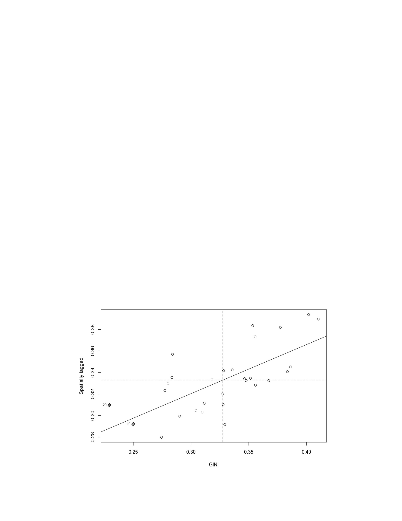
provinces or municipalities shown in quadrant 1) and of low-low value of the Gini coefficient (9

provinces or municipalities shown in quadrant 3). In 2014, 19 of the 29 administrative units in

China reveal a positive association ─ 10 provinces or municipalities with a high-high value of

the Gini coefficient and 9 provinces or municipalities with a low-low value of the Gini

coefficient (Figure 5). In brief, the Moran scatterplots indicate two types of spatial

autocorrelation, a spatial clustering of high-high values of the Gini coefficient and a spatial

clustering of low-low values of the Gini coefficient, indicating positive spatial autocorrelation.

Another finding from the Moran scatterplot in 1998 is, as expected, a regional polarization

between coast and inland provinces, indicating Western inland-provinces in the spatial clustering

of high-high values of the Gini coefficient and Eastern coast-provinces in the spatial clustering of

low-low values of the Gini coefficient. In 2014, however, the Moran scatterplot does not show

regional polarization between coast and inland provinces. Also, the slope of the Moran

scatterplot in 2014 is smaller (or flatter) than in 1998, indicating the degree of spatial dependence

decreases from 1998 to 2014. This is consistent with the decline in the Gini reported in Table 3.2.

Figure 3.4: Moran scatterplots for Gini coefficient in 1998

Figure 3.5: Moran scatterplots for Gini coefficient in 2014

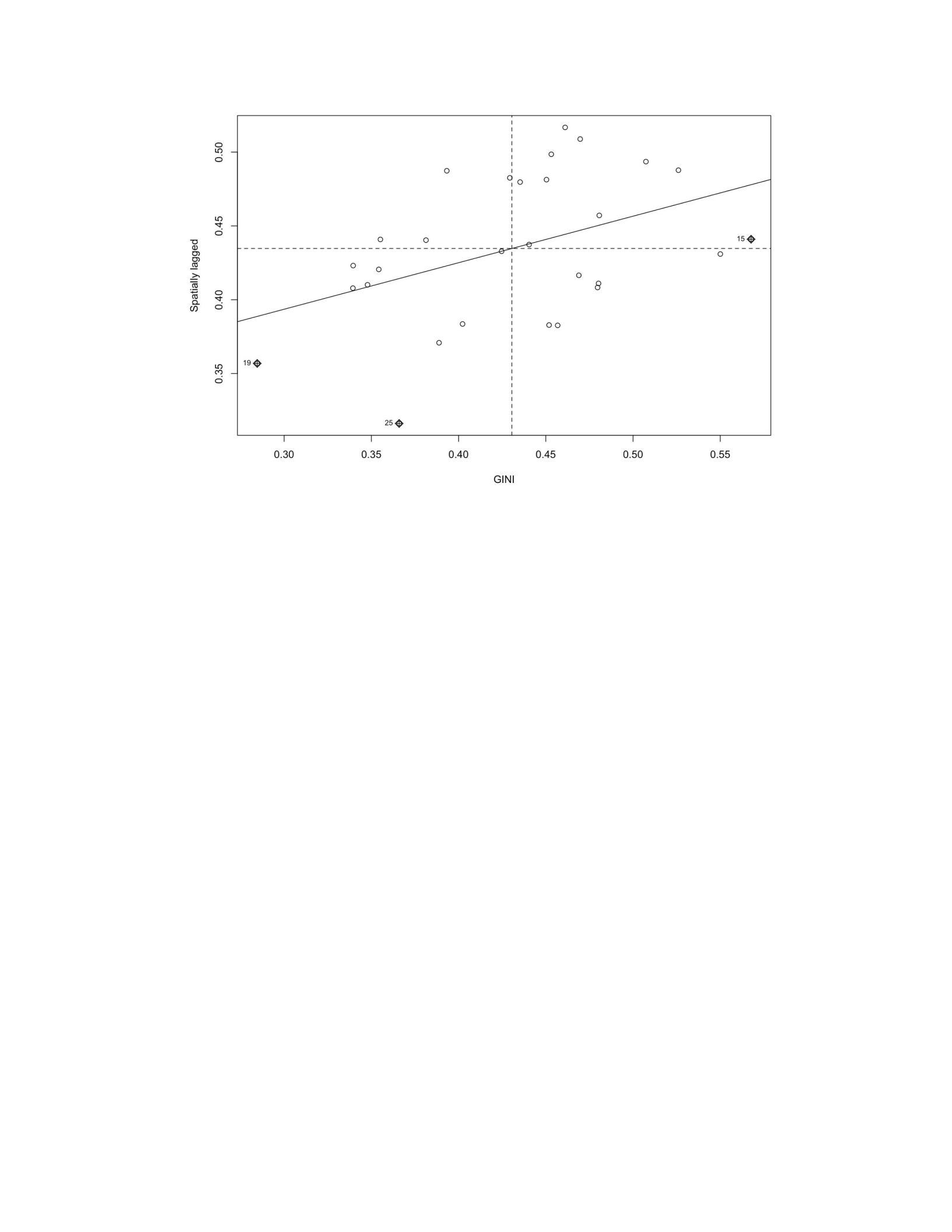
3.4.3 Cross-Sectional Spatial Model

In this section, we examine the cross-sectional spatial model for 1998, 2003, 2008 and

2013. First, a simple OLS (Ordinary Least Squares) regression was estimated and its residuals are

used to determine whether any specific spatial model is needed. If the Moran test of OLS residuals

shows spatial dependence, we must proceed to examine spatial models. Table 3.4 presents the

OLS estimation results with provincial data without controlling for spatial dependence. All

financial indicators are positive but not significant in 1998 is significant, while GDP per capita is

significant at the 5% significance level and has a negative impact on the Gini coefficient. The

direction of the effect of GDP per capita on the Gini coefficient is intuitive at first glance. For the

data sample in 2003, total deposit to provincial GDP and total loan to provincial GDP are

statistically significant and their signs are positive. In addition, the direction of the effect of

educational attainment on the Gini coefficient is initially intuitive since in general it is expected

that the effect of educational attainment on the Gini coefficient is negative. To check the necessity

of using a spatial model for China’s income inequality analysis, we conduct the Moran’s test on

the OLS residuals. The results are presented in Table 3.4. The p-values of the Moran’s I statistic

indicate the rejection of the null hypothesis for all three financial measures in 1998. Furthermore,

the null hypothesis is rejected for financial intermediation to provincial GDP and total deposit to

provincial GDP in 2003 and for all three financial measures in 2008, while the Moran test fails to

reject for all three financial measures in 2013. Thus, there are indications that spatial dependences

matter in the sample data from 1998, 2003, and 2008 and that spatial models should be estimated.

As mentioned, there are various ways that spatial dependence may enter the model. To

determine the type of dependence, we use the Lagrange Multiplier (LM) test to find the most

suitable spatial model. There are five different types of LM tests: (1) LMerr: the LM test for error

dependence; (2) LMlag: the LM test for missing spatially lagged dependent variable; (3)

RLMerr: the robust LM error that investigates for spatial error dependence in the possible of

presence of a missing lagged dependent variable; (4) RLMlag: the robust LM lag that

investigates for spatially lagged dependent variable; and (5) SARMA, which tests for both lag

and a moving average error. The robust LM tests enable us to understand what type of spatial

dependence captures the data best. Table 3.4 shows that LMlag and RLMlag are significant at the

5% significance level, while SARMA is significant at the 10% significance level for the dataset

from 1998, indicating the presence of spatial dependence, telling us that SARAR or the spatial

lag model should be applied to handle spatial dependence for the sample data from 1998.

Similarly, the spatial lag model is selected for the financial intermediation to provincial GDP for

2003 based on the LM test. However, although the global Moran test on the 2008 data rejects the

null hypothesis that there is no spatial dependence in the model, the LM test does not specify a

suitable spatial model.

Table 3.4: The OLS estimations, Moran’s I, and LM test (Dependent

Variable: Gini coefficient)

1998 2003

f_gdp 5.81 36.03

(0.19) (1.01)

d_gdp 3.52

(1.03)

3.22*

(1.93)

l_gdp 2.14

(0.72)

4.47**

(2.34)

lgdp_ca -5.55** (-

2.72)

-5.02** (-

2.48)

-5.22** (-

2.57)

-6.50*** (-

3.03)

-5.34** (-

2.50)

-5.58** (-

2.76)

open 3.75

(1.06)

1.61

(0.40)

3.34

(0.95)

2.75

(1.04)

1.09

(0.40)

1.89

(0.76)

edu -22.05

(-1.19)

-41.36

(-1.60)

-24.78

(-1.44)

-29.05** (-

2.55)

-40.14*** (-

3.15)

-36.45***

(-3.46)

Intercept 81.08***

(4.74)

73.96***

(4.13)

76.50***

(4.28)

100.69***

(5.37)

88.19***

(4.61)

89.33***

(4.95)

Moran’s I 0.22** 0.14** 0.14** 0.28*** 0.17** 0.08

LMerr 2.36 0.98 0.98 3.71* 1.43

LMlag 4.20** 2.79* 3.20* 7.12*** 4.37**

RLMerr 0.58 1.61 1.78 0.17 0.82

RLMlag 2.42** 3.42* 3.99** 3.58* 3.77*

SARMA 4.78* 4.40 4.98* 7.29** 5.20*

2008 2013

f_gdp 8.68

(0.26)

26.35

(0.44)

d_gdp 0.50 -0.63

(0.34) (-0.27)

l_gdp 1.07

(0.48)

1.32

(0.35)

lgdp_ca -4.14*

(-1.97)

-3.89*

(-1.71)

-3.99*

(-1.87)

-2.33

(-0.52)

-2.93

(-0.61)

-2.33

(-0.52)

open -0.48

(-0.21)

-0.59

(-0.26)

-0.61

(-0.29)

-2.14

(-0.46)

-0.16

(-0.03)

-1.62

(-0.38)

edu -22.84** (-

2.66)

-23.96** (-

2.47)

-23.31** (-

2.74)

-32.50* (-

2.05)

-29.40* (-

1.75)

-30.97* (-

1.99)

Intercept 85.49***

(4.244)

82.81***

(3.73)

83.45***

(4.03)

72.26

(1.57)

80.11

(1.59)

71.86

(1.55)

Moran’s I 0.13* 0.11* 0.13* -0.06 -0.03 -0.06

LMerr 0.76 0.56 0.82

LMlag 1.98 1.83 1.95

RLMerr 0.46 0.67 0.30

RLMlag 1.69 1.94 1.43

SARMA 2.45 2.50 2.25

Note: ***, **, and * indicates significance at the 1%, 5%, and 10% level, respectively. The numbers in parentheses

are t-statistics.

The estimation results of the spatial regression model on the effect of financial

development on income inequality are reported for 1998 and 2003 in Table 3.5. First, in the

sample data from 1998, the spatial lag and error model shows that the association between the

ratio of financial intermediation to provincial GDP and income inequality is positive but

insignificant. The spatial lag dependence, 𝜌, is positively significant at the 1% significance level,

while the spatial error dependence, 𝜆, is negatively significant. In addition, the Moran test results

after estimating the spatial model shows that there is no more spatial dependence in the residuals

of the spatial model with the sample data from 1998. The second finding is that the spatial lag

dependence is positively significant at the 1% significance level, while spatial error dependence

is negatively significant. However, the relationship between financial development and income

inequality in 2003 is insignificant.

As for the control variables, an initial finding is the effect of GDP per capita on income

inequality. In the sample data from 1998, the effect of GDP per capita is insignificant for all

estimation models. Additionally, the effect of GDP per capita is significantly negative at the 1%

and 5% significance levels, respectively, for the sample data from 2003. Another control

variable, educational attainment is significant at the 10% and 5% significance levels and its sign

is negative in 2003. The direction of the effect of educational attainment on the Gini coefficient

is quite reasonable because an increase in educational attainment leads a reduction in income

inequality.

Table 3.5: Spatial Model Estimations: SARAR (1,1) models

(Dependent Variable: Gini Coefficient)

1998 2003

F_gdp -3.25

(-0.14)

-4.06

(-0.21)

D_gdp 1.91

(0.86)

1.25

(1.16)

L_gdp 1.83

(0.95)

Lgdp_ca -3.11*

(-1.95)

-2.85** (-

2.02)

-2.90** (-

2.08)

-3.10*** (-

2.19)

-2.77** (-

2.04)

Open 2.64

(1.02)

1.63

(0.66)

2.64

(1.16)

1.40

(0.87)

0.57

(0.37)

Edu -12.48

(-0.95))

-23.33

(-1.35)

-16.64

(-1.41)

-10.68* (-

1.72)

-17.63** (-

2.34)

Intercept 36.67**

(2.07)

32.62

(2.07)

33.01

(2.12)

37.68**

(2.39)

35.04**

(2.30)

Rho 0.71***

(3.70)

0.71***

(4.13)

0.71***

(4.16)

0.78***

(7.05)

0.75***

(6.22)

Lambda -0.49

(-1.26)

-0.65*

(-1.93)

-0.67** (-

2.06)

-0.79*** (-

3.10)

-0.84*** (-

3.48)

Note: ***, **, and * indicates significance at the 1%, 5%, and 10% level, respectively. The numbers in parentheses

are z-statistics.

Table 3.6: Direct & Indirect effects (1998)

f_gdp d_gdp l_gdp

Direct Indirect Total Direct Indirect Total Direct Indirect Total

F_gdp -4.04 -6.98 -11.02

D_gdp 2.39 4.24 6.63

L_gdp 2.28 3.97 6.24

Lgdp_ca -3.87 -6.67 -10.54 -3.57 -6.32 -9.89 -3.62 -6.29 -9.91

Open 3.29 5.67 8.96 2.04 3.62 5.66 3.29 5.74 9.03

Edu -15.54 -26.82 -42.36 -29.22 -51.73 -80.95 -20.77 -36.15 -56.92

Table 3.7: Direct & Indirect effects: (2003)

f_gdp d_gdp

ECN 360-Introduction causal effects among economic

Students also viewed