


The Concept of Utility
Why do you buy the goods and services you do? It must be because they provide you with
satisfaction—you feel better off because you have purchased them. Economists call this
satisfaction utility.
The concept of utility is an elusive one. A person who consumes a good such as peaches gains
utility from eating the peaches. But we cannot measure this utility the same way we can
measure a peach’s weight or calorie content. There is no scale we can use to determine the
quantity of utility a peach generates.
Francis Edgeworth, one of the most important contributors to the theory of consumer behavior,
imagined a device he called a hedonimeter (after hedonism, the pursuit of pleasure):
“[L]et there be granted to the science of pleasure what is granted to the science of energy; to
imagine an ideally perfect instrument, a psychophysical machine, continually registering the
height of pleasure experienced by an individual…. From moment to moment the hedonimeter
varies; the delicate index now flickering with the flutter of passions, now steadied by
intellectual activity, now sunk whole hours in the neighborhood of zero, or momentarily
springing up towards infinity.”Francis Y. Edgeworth, Mathematical Psychics: An Essay on the
Application of Mathematics to the Moral Sciences (New York: Augustus M. Kelley, 1967), p.
101. First Published 1881.
Perhaps some day a hedonimeter will be invented. The utility it measures will not be a
characteristic of particular goods, but rather of each consumer’s reactions to those goods. The
utility of a peach exists not in the peach itself, but in the preferences of the individual
consuming the peach. One consumer may wax ecstatic about a peach; another may say it tastes
OK.

When we speak of maximizing utility, then, we are speaking of the maximization of something
we cannot measure. We assume, however, that each consumer acts as if he or she can measure
utility and arranges consumption so that the utility gained is as high as possible.
Total Utility
If we could measure utility, total utility would be the number of units of utility that a consumer
gains from consuming a given quantity of a good, service, or activity during a particular time
period. The higher a consumer’s total utility, the greater that consumer’s level of satisfaction.
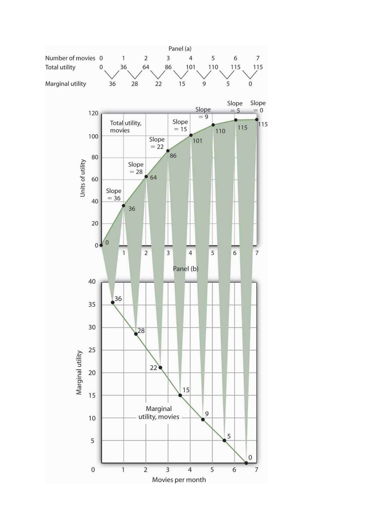
Panel (a) of Figure 7.1 "Total Utility and Marginal Utility Curves" shows the total utility Henry
Higgins obtains from attending movies. In drawing his total utility curve, we are imagining that
he can measure his total utility. The total utility curve shows that when Mr. Higgins attends no
movies during a month, his total utility from attending movies is zero. As he increases the
number of movies he sees, his total utility rises. When he consumes 1 movie, he obtains 36
units of utility. When he consumes 4 movies, his total utility is 101. He achieves the maximum
level of utility possible, 115, by seeing 6 movies per month. Seeing a seventh movie adds
nothing to his total utility.
Figure 7.1 Total Utility and Marginal Utility Curves
Number
of
movies
0
1
2 3
4
Total
utility
0
vs
yr
+f
Marginal
utility
36
28
22
15
9
Units
of
utility
Marginal
utility
120
2
o
S
g
b
3S
N
S
35
30
25
20
15
10
Panel
(a)
=
110
6
115
7
115
5
0
Marginal
utility,
movies
3
4
Movies
per
month

Panel (a) shows Henry Higgins’s total utility curve for attending movies. It rises as the number
of movies increases, reaching a maximum of 115 units of utility at 6 movies per month. Marginal
utility is shown in Panel (b); it is the slope of the total utility curve. Because the slope of the
total utility curve declines as the number of movies increases, the marginal utility curve is
downward sloping.
Mr. Higgins’s total utility rises at a decreasing rate. The rate of increase is given by the slope
of the total utility curve, which is reported in Panel (a) of Figure 7.1 "Total Utility and Marginal
Utility Curves" as well. The slope of the curve between 0 movies and 1 movie is 36 because
utility rises by this amount when Mr. Higgins sees his first movie in the month. It is 28 between
1 and 2 movies, 22 between 2 and 3, and so on. The slope between 6 and 7 movies is zero; the
total utility curve between these two quantities is horizontal.
Marginal Utility
The amount by which total utility rises with consumption of an additional unit of a good,
service, or activity, all other things unchanged, is marginal utility. The first movie Mr. Higgins
sees increases his total utility by 36 units. Hence, the marginal utility of the first movie is 36.
The second increases his total utility by 28 units; its marginal utility is 28. The seventh movie
does not increase his total utility; its marginal utility is zero. Notice that in the table marginal
utility is listed between the columns for total utility because, similar to other marginal concepts,
marginal utility is the change in utility as we go from one quantity to the next. Mr. Higgins’s
marginal utility curve is plotted in Panel (b) of Figure 7.1 "Total Utility and Marginal Utility
Curves" The values for marginal utility are plotted midway between the numbers of movies
attended. The marginal utility curve is downward sloping; it shows that Mr. Higgins’s marginal
utility for movies declines as he consumes more of them.

Mr. Higgins’s marginal utility from movies is typical of all goods and services. Suppose that
you are really thirsty and you decide to consume a soft drink. Consuming the drink increases
your utility, probably by a lot. Suppose now you have another. That second drink probably
increases your utility by less than the first. A third would increase your utility by still less. This
tendency of marginal utility to decline beyond some level of consumption during a period is
called the law of diminishing marginal utility. This law implies that all goods and services
eventually will have downward-sloping marginal utility curves. It is the law that lies behind
the negatively sloped marginal benefit curve for consumer choices that we examined in the
chapter on markets, maximizers, and efficiency.
One way to think about this effect is to remember the last time you ate at an “all you can eat”
cafeteria-style restaurant. Did you eat only one type of food? Did you consume food without
limit? No, because of the law of diminishing marginal utility. As you consumed more of one
kind of food, its marginal utility fell. You reached a point at which the marginal utility of
another dish was greater, and you switched to that. Eventually, there was no food whose
marginal utility was great enough to make it worth eating, and you stopped.
What if the law of diminishing marginal utility did not hold? That is, what would life be like
in a world of constant or increasing marginal utility? In your mind go back to the cafeteria and
imagine that you have rather unusual preferences: Your favorite food is creamed spinach. You
start with that because its marginal utility is highest of all the choices before you in the cafeteria.
As you eat more, however, its marginal utility does not fall; it remains higher than the marginal
utility of any other option. Unless eating more creamed spinach somehow increases your
marginal utility for some other food, you will eat only creamed spinach. And until you have
reached the limit of your body’s capacity (or the restaurant manager’s patience), you will not
stop. Failure of marginal utility to diminish would thus lead to extraordinary levels of
consumption of a single good to the exclusion of all others. Since we do not observe that

happening, it seems reasonable to assume that marginal utility falls beyond some level of
consumption.
Maximizing Utility
Economists assume that consumers behave in a manner consistent with the maximization of
utility. To see how consumers do that, we will put the marginal decision rule to work. First,
however, we must reckon with the fact that the ability of consumers to purchase goods and
services is limited by their budgets.
The Budget Constraint
The total utility curve in Figure 7.1 "Total Utility and Marginal Utility Curves" shows that Mr.
Higgins achieves the maximum total utility possible from movies when he sees six of them
each month. It is likely that his total utility curves for other goods and services will have much
the same shape, reaching a maximum at some level of consumption. We assume that the goal
of each consumer is to maximize total utility. Does that mean a person will consume each good
at a level that yields the maximum utility possible?
The answer, in general, is no. Our consumption choices are constrained by the income available
to us and by the prices we must pay. Suppose, for example, that Mr. Higgins can spend just $25
per month for entertainment and that the price of going to see a movie is $5. To achieve the
maximum total utility from movies, Mr. Higgins would have to exceed his entertainment
budget. Since we assume that he cannot do that, Mr. Higgins must arrange his consumption so
that his total expenditures do not exceed his budget constraint: a restriction that total spending
cannot exceed the budget available.
Suppose that in addition to movies, Mr. Higgins enjoys concerts, and the average price of a
concert ticket is $10. He must select the number of movies he sees and concerts he attends so
that his monthly spending on the two goods does not exceed his budget.

Individuals may, of course, choose to save or to borrow. When we allow this possibility, we
consider the budget constraint not just for a single period of time but for several periods. For
example, economists often examine budget constraints over a consumer’s lifetime. A consumer
may in some years save for future consumption and in other years borrow on future income for
present consumption. Whatever the time period, a consumer’s spending will be constrained by
his or her budget.
To simplify our analysis, we shall assume that a consumer’s spending in any one period is
based on the budget available in that period. In this analysis consumers neither save nor borrow.
We could extend the analysis to cover several periods and generate the same basic results that
we shall establish using a single period. We will also carry out our analysis by looking at the
consumer’s choices about buying only two goods. Again, the analysis could be extended to
cover more goods and the basic results would still hold.
Applying the Marginal Decision Rule
Because consumers can be expected to spend the budget they have, utility maximization is a
matter of arranging that spending to achieve the highest total utility possible. If a consumer
decides to spend more on one good, he or she must spend less on another in order to satisfy the
budget constraint.
The marginal decision rule states that an activity should be expanded if its marginal benefit
exceeds its marginal cost. The marginal benefit of this activity is the utility gained by spending
an additional $1 on the good. The marginal cost is the utility lost by spending $1 less on another
good.
How much utility is gained by spending another $1 on a good? It is the marginal utility of the
good divided by its price. The utility gained by spending an additional dollar on good X, for
example, is

MUXPX
This additional utility is the marginal benefit of spending another $1 on the good.
Suppose that the marginal utility of good X is 4 and that its price is $2. Then an extra $1 spent
on X buys 2 additional units of utility (MUX/PX=4/2=2 ). If the marginal utility of good X is
1 and its price is $2, then an extra $1 spent on X buys 0.5 additional units of utility
(MUX/PX=1/2=0.5 ).
The loss in utility from spending $1 less on another good or service is calculated the same way:
as the marginal utility divided by the price. The marginal cost to the consumer of spending $1
less on a good is the loss of the additional utility that could have been gained from spending
that $1 on the good.
Suppose a consumer derives more utility by spending an additional $1 on good X rather than
on good Y:
Equation 7.1
MUXPX>MUYPY
The marginal benefit of shifting $1 from good Y to the consumption of good X exceeds the
marginal cost. In terms of utility, the gain from spending an additional $1 on good X exceeds
the loss in utility from spending $1 less on good Y. The consumer can increase utility by shifting
spending from Y to X.
As the consumer buys more of good X and less of good Y, however, the marginal utilities of
the two goods will change. The law of diminishing marginal utility tells us that the marginal
utility of good X will fall as the consumer consumes more of it; the marginal utility of good Y
will rise as the consumer consumes less of it. The result is that the value of the left-hand side
of Equation 7.1 will fall and the value of the right-hand side will rise as the consumer shifts

spending from Y to X. When the two sides are equal, total utility will be maximized. In terms
of the marginal decision rule, the consumer will have achieved a solution at which the marginal
benefit of the activity (spending more on good X) is equal to the marginal cost:
Equation 7.2
MUXPX=MUYPY
We can extend this result to all goods and services a consumer uses. Utility maximization
requires that the ratio of marginal utility to price be equal for all of them, as suggested
in Equation 7.3:
Equation 7.3
MUAPA=MUBPB=MUCPC=...=MUnPn
Equation 7.3 states the utility-maximizing condition: Utility is maximized when total outlays
equal the budget available and when the ratios of marginal utilities to prices are equal for all
goods and services.
Consider, for example, the shopper introduced in the opening of this chapter. In shifting from
cookies to ice cream, the shopper must have felt that the marginal utility of spending an
additional dollar on ice cream exceeded the marginal utility of spending an additional dollar on
cookies. In terms of Equation 7.1, if good X is ice cream and good Y is cookies, the shopper
will have lowered the value of the left-hand side of the equation and moved toward the utility-
maximizing condition, as expressed by Equation 7.1.
The Problem of Divisibility
If we are to apply the marginal decision rule to utility maximization, goods must be divisible;
that is, it must be possible to buy them in any amount. Otherwise we cannot meaningfully speak

of spending $1 more or $1 less on them. Strictly speaking, however, few goods are completely
divisible.
Even a small purchase, such as an ice cream bar, fails the strict test of being divisible; grocers
generally frown on requests to purchase one-half of a $2 ice cream bar if the consumer wants
to spend an additional dollar on ice cream. Can a consumer buy a little more movie admission,
to say nothing of a little more car?
In the case of a car, we can think of the quantity as depending on characteristics of the car itself.
A car with a compact disc player could be regarded as containing “more car” than one that has
only a cassette player. Stretching the concept of quantity in this manner does not entirely solve
the problem. It is still difficult to imagine that one could purchase “more car” by spending $1
more.
Remember, though, that we are dealing with a model. In the real world, consumers may not be
able to satisfy Equation 7.3 precisely. The model predicts, however, that they will come as close
to doing so as possible.
Marginal Utility
The amount by which total utility rises with consumption of an additional unit of a good,
service, or activity, all other things unchanged, is marginal utility. The first movie Mr. Higgins
sees increases his total utility by 36 units. Hence, the marginal utility of the first movie is 36.
The second increases his total utility by 28 units; its marginal utility is 28. The seventh movie
does not increase his total utility; its marginal utility is zero. Notice that in the table marginal
utility is listed between the columns for total utility because, similar to other marginal concepts,
marginal utility is the change in utility as we go from one quantity to the next. Mr. Higgins’s
marginal utility curve is plotted in Panel (b) of Figure 7.1 "Total Utility and Marginal Utility
Curves" The values for marginal utility are plotted midway between the numbers of movies

attended. The marginal utility curve is downward sloping; it shows that Mr. Higgins’s marginal
utility for movies declines as he consumes more of them.
Mr. Higgins’s marginal utility from movies is typical of all goods and services. Suppose that
you are really thirsty and you decide to consume a soft drink. Consuming the drink increases
your utility, probably by a lot. Suppose now you have another. That second drink probably
increases your utility by less than the first. A third would increase your utility by still less. This
tendency of marginal utility to decline beyond some level of consumption during a period is
called the law of diminishing marginal utility. This law implies that all goods and services
eventually will have downward-sloping marginal utility curves. It is the law that lies behind
the negatively sloped marginal benefit curve for consumer choices that we examined in the
chapter on markets, maximizers, and efficiency.
One way to think about this effect is to remember the last time you ate at an “all you can eat”
cafeteria-style restaurant. Did you eat only one type of food? Did you consume food without
limit? No, because of the law of diminishing marginal utility. As you consumed more of one
kind of food, its marginal utility fell. You reached a point at which the marginal utility of
another dish was greater, and you switched to that. Eventually, there was no food whose
marginal utility was great enough to make it worth eating, and you stopped.
What if the law of diminishing marginal utility did not hold? That is, what would life be like
in a world of constant or increasing marginal utility? In your mind go back to the cafeteria and
imagine that you have rather unusual preferences: Your favorite food is creamed spinach. You
start with that because its marginal utility is highest of all the choices before you in the cafeteria.
As you eat more, however, its marginal utility does not fall; it remains higher than the marginal
utility of any other option. Unless eating more creamed spinach somehow increases your
marginal utility for some other food, you will eat only creamed spinach. And until you have

reached the limit of your body’s capacity (or the restaurant manager’s patience), you will not
stop. Failure of marginal utility to diminish would thus lead to extraordinary levels of
consumption of a single good to the exclusion of all others. Since we do not observe that
happening, it seems reasonable to assume that marginal utility falls beyond some level of
consumption.
Maximizing Utility
Economists assume that consumers behave in a manner consistent with the maximization of
utility. To see how consumers do that, we will put the marginal decision rule to work. First,
however, we must reckon with the fact that the ability of consumers to purchase goods and
services is limited by their budgets.
The Budget Constraint
The total utility curve in Figure 7.1 "Total Utility and Marginal Utility Curves" shows that Mr.
Higgins achieves the maximum total utility possible from movies when he sees six of them
each month. It is likely that his total utility curves for other goods and services will have much
the same shape, reaching a maximum at some level of consumption. We assume that the goal
of each consumer is to maximize total utility. Does that mean a person will consume each good
at a level that yields the maximum utility possible?
The answer, in general, is no. Our consumption choices are constrained by the income available
to us and by the prices we must pay. Suppose, for example, that Mr. Higgins can spend just $25
per month for entertainment and that the price of going to see a movie is $5. To achieve the
maximum total utility from movies, Mr. Higgins would have to exceed his entertainment
budget. Since we assume that he cannot do that, Mr. Higgins must arrange his consumption so
that his total expenditures do not exceed his budget constraint: a restriction that total spending
cannot exceed the budget available.

Suppose that in addition to movies, Mr. Higgins enjoys concerts, and the average price of a
concert ticket is $10. He must select the number of movies he sees and concerts he attends so
that his monthly spending on the two goods does not exceed his budget.
Individuals may, of course, choose to save or to borrow. When we allow this possibility, we
consider the budget constraint not just for a single period of time but for several periods. For
example, economists often examine budget constraints over a consumer’s lifetime. A consumer
may in some years save for future consumption and in other years borrow on future income for
present consumption. Whatever the time period, a consumer’s spending will be constrained by
his or her budget.
To simplify our analysis, we shall assume that a consumer’s spending in any one period is
based on the budget available in that period. In this analysis consumers neither save nor borrow.
We could extend the analysis to cover several periods and generate the same basic results that
we shall establish using a single period. We will also carry out our analysis by looking at the
consumer’s choices about buying only two goods. Again, the analysis could be extended to
cover more goods and the basic results would still hold.
Applying the Marginal Decision Rule
Because consumers can be expected to spend the budget they have, utility maximization is a
matter of arranging that spending to achieve the highest total utility possible. If a consumer
decides to spend more on one good, he or she must spend less on another in order to satisfy the
budget constraint.
The marginal decision rule states that an activity should be expanded if its marginal benefit
exceeds its marginal cost. The marginal benefit of this activity is the utility gained by spending
an additional $1 on the good. The marginal cost is the utility lost by spending $1 less on another
good.

How much utility is gained by spending another $1 on a good? It is the marginal utility of the
good divided by its price. The utility gained by spending an additional dollar on good X, for
example, is
MUXPX
This additional utility is the marginal benefit of spending another $1 on the good.
Suppose that the marginal utility of good X is 4 and that its price is $2. Then an extra $1 spent
on X buys 2 additional units of utility (MUX/PX=4/2=2 ). If the marginal utility of good X is
1 and its price is $2, then an extra $1 spent on X buys 0.5 additional units of utility
(MUX/PX=1/2=0.5 ).
The loss in utility from spending $1 less on another good or service is calculated the same way:
as the marginal utility divided by the price. The marginal cost to the consumer of spending $1
less on a good is the loss of the additional utility that could have been gained from spending
that $1 on the good.
Suppose a consumer derives more utility by spending an additional $1 on good X rather than
on good Y:
Equation 7.1
MUXPX>MUYPY
The marginal benefit of shifting $1 from good Y to the consumption of good X exceeds the
marginal cost. In terms of utility, the gain from spending an additional $1 on good X exceeds
the loss in utility from spending $1 less on good Y. The consumer can increase utility by shifting
spending from Y to X.
As the consumer buys more of good X and less of good Y, however, the marginal utilities of
the two goods will change. The law of diminishing marginal utility tells us that the marginal

utility of good X will fall as the consumer consumes more of it; the marginal utility of good Y
will rise as the consumer consumes less of it. The result is that the value of the left-hand side
of Equation 7.1 will fall and the value of the right-hand side will rise as the consumer shifts
spending from Y to X. When the two sides are equal, total utility will be maximized. In terms
of the marginal decision rule, the consumer will have achieved a solution at which the marginal
benefit of the activity (spending more on good X) is equal to the marginal cost:
Equation 7.2
MUXPX=MUYPY
We can extend this result to all goods and services a consumer uses. Utility maximization
requires that the ratio of marginal utility to price be equal for all of them, as suggested
in Equation 7.3:
Equation 7.3
MUAPA=MUBPB=MUCPC=...=MUnPn
Equation 7.3 states the utility-maximizing condition: Utility is maximized when total outlays
equal the budget available and when the ratios of marginal utilities to prices are equal for all
goods and services.
Consider, for example, the shopper introduced in the opening of this chapter. In shifting from
cookies to ice cream, the shopper must have felt that the marginal utility of spending an
additional dollar on ice cream exceeded the marginal utility of spending an additional dollar on
cookies. In terms of Equation 7.1, if good X is ice cream and good Y is cookies, the shopper
will have lowered the value of the left-hand side of the equation and moved toward the utility-
maximizing condition, as expressed by Equation 7.1.
The Problem of Divisibility

If we are to apply the marginal decision rule to utility maximization, goods must be divisible;
that is, it must be possible to buy them in any amount. Otherwise we cannot meaningfully speak
of spending $1 more or $1 less on them. Strictly speaking, however, few goods are completely
divisible.
Even a small purchase, such as an ice cream bar, fails the strict test of being divisible; grocers
generally frown on requests to purchase one-half of a $2 ice cream bar if the consumer wants
to spend an additional dollar on ice cream. Can a consumer buy a little more movie admission,
to say nothing of a little more car?
In the case of a car, we can think of the quantity as depending on characteristics of the car itself.
A car with a compact disc player could be regarded as containing “more car” than one that has
only a cassette player. Stretching the concept of quantity in this manner does not entirely solve
the problem. It is still difficult to imagine that one could purchase “more car” by spending $1
more.
Remember, though, that we are dealing with a model. In the real world, consumers may not be
able to satisfy Equation 7.3 precisely. The model predicts, however, that they will come as close
to doing so as possible.
Marginal Utility
The amount by which total utility rises with consumption of an additional unit of a good,
service, or activity, all other things unchanged, is marginal utility. The first movie Mr. Higgins
sees increases his total utility by 36 units. Hence, the marginal utility of the first movie is 36.
The second increases his total utility by 28 units; its marginal utility is 28. The seventh movie
does not increase his total utility; its marginal utility is zero. Notice that in the table marginal
utility is listed between the columns for total utility because, similar to other marginal concepts,
marginal utility is the change in utility as we go from one quantity to the next. Mr. Higgins’s

marginal utility curve is plotted in Panel (b) of Figure 7.1 "Total Utility and Marginal Utility
Curves" The values for marginal utility are plotted midway between the numbers of movies
attended. The marginal utility curve is downward sloping; it shows that Mr. Higgins’s marginal
utility for movies declines as he consumes more of them.
Mr. Higgins’s marginal utility from movies is typical of all goods and services. Suppose that
you are really thirsty and you decide to consume a soft drink. Consuming the drink increases
your utility, probably by a lot. Suppose now you have another. That second drink probably
increases your utility by less than the first. A third would increase your utility by still less. This
tendency of marginal utility to decline beyond some level of consumption during a period is
called the law of diminishing marginal utility. This law implies that all goods and services
eventually will have downward-sloping marginal utility curves. It is the law that lies behind
the negatively sloped marginal benefit curve for consumer choices that we examined in the
chapter on markets, maximizers, and efficiency.
One way to think about this effect is to remember the last time you ate at an “all you can eat”
cafeteria-style restaurant. Did you eat only one type of food? Did you consume food without
limit? No, because of the law of diminishing marginal utility. As you consumed more of one
kind of food, its marginal utility fell. You reached a point at which the marginal utility of
another dish was greater, and you switched to that. Eventually, there was no food whose
marginal utility was great enough to make it worth eating, and you stopped.
What if the law of diminishing marginal utility did not hold? That is, what would life be like
in a world of constant or increasing marginal utility? In your mind go back to the cafeteria and
imagine that you have rather unusual preferences: Your favorite food is creamed spinach. You
start with that because its marginal utility is highest of all the choices before you in the cafeteria.
As you eat more, however, its marginal utility does not fall; it remains higher than the marginal

utility of any other option. Unless eating more creamed spinach somehow increases your
marginal utility for some other food, you will eat only creamed spinach. And until you have
reached the limit of your body’s capacity (or the restaurant manager’s patience), you will not
stop. Failure of marginal utility to diminish would thus lead to extraordinary levels of
consumption of a single good to the exclusion of all others. Since we do not observe that
happening, it seems reasonable to assume that marginal utility falls beyond some level of
consumption.
Maximizing Utility
Economists assume that consumers behave in a manner consistent with the maximization of
utility. To see how consumers do that, we will put the marginal decision rule to work. First,
however, we must reckon with the fact that the ability of consumers to purchase goods and
services is limited by their budgets.
The Budget Constraint
The total utility curve in Figure 7.1 "Total Utility and Marginal Utility Curves" shows that Mr.
Higgins achieves the maximum total utility possible from movies when he sees six of them
each month. It is likely that his total utility curves for other goods and services will have much
the same shape, reaching a maximum at some level of consumption. We assume that the goal
of each consumer is to maximize total utility. Does that mean a person will consume each good
at a level that yields the maximum utility possible?
The answer, in general, is no. Our consumption choices are constrained by the income available
to us and by the prices we must pay. Suppose, for example, that Mr. Higgins can spend just $25
per month for entertainment and that the price of going to see a movie is $5. To achieve the
maximum total utility from movies, Mr. Higgins would have to exceed his entertainment
budget. Since we assume that he cannot do that, Mr. Higgins must arrange his consumption so

that his total expenditures do not exceed his budget constraint: a restriction that total spending
cannot exceed the budget available.
Suppose that in addition to movies, Mr. Higgins enjoys concerts, and the average price of a
concert ticket is $10. He must select the number of movies he sees and concerts he attends so
that his monthly spending on the two goods does not exceed his budget.
Individuals may, of course, choose to save or to borrow. When we allow this possibility, we
consider the budget constraint not just for a single period of time but for several periods. For
example, economists often examine budget constraints over a consumer’s lifetime. A consumer
may in some years save for future consumption and in other years borrow on future income for
present consumption. Whatever the time period, a consumer’s spending will be constrained by
his or her budget.
To simplify our analysis, we shall assume that a consumer’s spending in any one period is
based on the budget available in that period. In this analysis consumers neither save nor borrow.
We could extend the analysis to cover several periods and generate the same basic results that
we shall establish using a single period. We will also carry out our analysis by looking at the
consumer’s choices about buying only two goods. Again, the analysis could be extended to
cover more goods and the basic results would still hold.
Applying the Marginal Decision Rule
Because consumers can be expected to spend the budget they have, utility maximization is a
matter of arranging that spending to achieve the highest total utility possible. If a consumer
decides to spend more on one good, he or she must spend less on another in order to satisfy the
budget constraint.
The marginal decision rule states that an activity should be expanded if its marginal benefit
exceeds its marginal cost. The marginal benefit of this activity is the utility gained by spending

an additional $1 on the good. The marginal cost is the utility lost by spending $1 less on another
good.
How much utility is gained by spending another $1 on a good? It is the marginal utility of the
good divided by its price. The utility gained by spending an additional dollar on good X, for
example, is
MUXPX
This additional utility is the marginal benefit of spending another $1 on the good.
Suppose that the marginal utility of good X is 4 and that its price is $2. Then an extra $1 spent
on X buys 2 additional units of utility (MUX/PX=4/2=2 ). If the marginal utility of good X is
1 and its price is $2, then an extra $1 spent on X buys 0.5 additional units of utility
(MUX/PX=1/2=0.5 ).
The loss in utility from spending $1 less on another good or service is calculated the same way:
as the marginal utility divided by the price. The marginal cost to the consumer of spending $1
less on a good is the loss of the additional utility that could have been gained from spending
that $1 on the good.
Suppose a consumer derives more utility by spending an additional $1 on good X rather than
on good Y:
Equation 7.1
MUXPX>MUYPY
The marginal benefit of shifting $1 from good Y to the consumption of good X exceeds the
marginal cost. In terms of utility, the gain from spending an additional $1 on good X exceeds
the loss in utility from spending $1 less on good Y. The consumer can increase utility by shifting
spending from Y to X.

As the consumer buys more of good X and less of good Y, however, the marginal utilities of
the two goods will change. The law of diminishing marginal utility tells us that the marginal
utility of good X will fall as the consumer consumes more of it; the marginal utility of good Y
will rise as the consumer consumes less of it. The result is that the value of the left-hand side
of Equation 7.1 will fall and the value of the right-hand side will rise as the consumer shifts
spending from Y to X. When the two sides are equal, total utility will be maximized. In terms
of the marginal decision rule, the consumer will have achieved a solution at which the marginal
benefit of the activity (spending more on good X) is equal to the marginal cost:
Equation 7.2
MUXPX=MUYPY
We can extend this result to all goods and services a consumer uses. Utility maximization
requires that the ratio of marginal utility to price be equal for all of them, as suggested
in Equation 7.3:
Equation 7.3
MUAPA=MUBPB=MUCPC=...=MUnPn
Equation 7.3 states the utility-maximizing condition: Utility is maximized when total outlays
equal the budget available and when the ratios of marginal utilities to prices are equal for all
goods and services.
Consider, for example, the shopper introduced in the opening of this chapter. In shifting from
cookies to ice cream, the shopper must have felt that the marginal utility of spending an
additional dollar on ice cream exceeded the marginal utility of spending an additional dollar on
cookies. In terms of Equation 7.1, if good X is ice cream and good Y is cookies, the shopper

will have lowered the value of the left-hand side of the equation and moved toward the utility-
maximizing condition, as expressed by Equation 7.1.
The Problem of Divisibility
If we are to apply the marginal decision rule to utility maximization, goods must be divisible;
that is, it must be possible to buy them in any amount. Otherwise we cannot meaningfully speak
of spending $1 more or $1 less on them. Strictly speaking, however, few goods are completely
divisible.
Even a small purchase, such as an ice cream bar, fails the strict test of being divisible; grocers
generally frown on requests to purchase one-half of a $2 ice cream bar if the consumer wants
to spend an additional dollar on ice cream. Can a consumer buy a little more movie admission,
to say nothing of a little more car?
In the case of a car, we can think of the quantity as depending on characteristics of the car itself.
A car with a compact disc player could be regarded as containing “more car” than one that has
only a cassette player. Stretching the concept of quantity in this manner does not entirely solve
the problem. It is still difficult to imagine that one could purchase “more car” by spending $1
more.
Remember, though, that we are dealing with a model. In the real world, consumers may not be
able to satisfy Equation 7.3 precisely. The model predicts, however, that they will come as close
to doing so as possible.
Marginal Utility
The amount by which total utility rises with consumption of an additional unit of a good,
service, or activity, all other things unchanged, is marginal utility. The first movie Mr. Higgins
sees increases his total utility by 36 units. Hence, the marginal utility of the first movie is 36.

The second increases his total utility by 28 units; its marginal utility is 28. The seventh movie
does not increase his total utility; its marginal utility is zero. Notice that in the table marginal
utility is listed between the columns for total utility because, similar to other marginal concepts,
marginal utility is the change in utility as we go from one quantity to the next. Mr. Higgins’s
marginal utility curve is plotted in Panel (b) of Figure 7.1 "Total Utility and Marginal Utility
Curves" The values for marginal utility are plotted midway between the numbers of movies
attended. The marginal utility curve is downward sloping; it shows that Mr. Higgins’s marginal
utility for movies declines as he consumes more of them.
Mr. Higgins’s marginal utility from movies is typical of all goods and services. Suppose that
you are really thirsty and you decide to consume a soft drink. Consuming the drink increases
your utility, probably by a lot. Suppose now you have another. That second drink probably
increases your utility by less than the first. A third would increase your utility by still less. This
tendency of marginal utility to decline beyond some level of consumption during a period is
called the law of diminishing marginal utility. This law implies that all goods and services
eventually will have downward-sloping marginal utility curves. It is the law that lies behind
the negatively sloped marginal benefit curve for consumer choices that we examined in the
chapter on markets, maximizers, and efficiency.
One way to think about this effect is to remember the last time you ate at an “all you can eat”
cafeteria-style restaurant. Did you eat only one type of food? Did you consume food without
limit? No, because of the law of diminishing marginal utility. As you consumed more of one
kind of food, its marginal utility fell. You reached a point at which the marginal utility of
another dish was greater, and you switched to that. Eventually, there was no food whose
marginal utility was great enough to make it worth eating, and you stopped.

What if the law of diminishing marginal utility did not hold? That is, what would life be like
in a world of constant or increasing marginal utility? In your mind go back to the cafeteria and
imagine that you have rather unusual preferences: Your favorite food is creamed spinach. You
start with that because its marginal utility is highest of all the choices before you in the cafeteria.
As you eat more, however, its marginal utility does not fall; it remains higher than the marginal
utility of any other option. Unless eating more creamed spinach somehow increases your
marginal utility for some other food, you will eat only creamed spinach. And until you have
reached the limit of your body’s capacity (or the restaurant manager’s patience), you will not
stop. Failure of marginal utility to diminish would thus lead to extraordinary levels of
consumption of a single good to the exclusion of all others. Since we do not observe that
happening, it seems reasonable to assume that marginal utility falls beyond some level of
consumption.
Maximizing Utility
Economists assume that consumers behave in a manner consistent with the maximization of
utility. To see how consumers do that, we will put the marginal decision rule to work. First,
however, we must reckon with the fact that the ability of consumers to purchase goods and
services is limited by their budgets.
The Budget Constraint
The total utility curve in Figure 7.1 "Total Utility and Marginal Utility Curves" shows that Mr.
Higgins achieves the maximum total utility possible from movies when he sees six of them
each month. It is likely that his total utility curves for other goods and services will have much
the same shape, reaching a maximum at some level of consumption. We assume that the goal
of each consumer is to maximize total utility. Does that mean a person will consume each good
at a level that yields the maximum utility possible?

The answer, in general, is no. Our consumption choices are constrained by the income available
to us and by the prices we must pay. Suppose, for example, that Mr. Higgins can spend just $25
per month for entertainment and that the price of going to see a movie is $5. To achieve the
maximum total utility from movies, Mr. Higgins would have to exceed his entertainment
budget. Since we assume that he cannot do that, Mr. Higgins must arrange his consumption so
that his total expenditures do not exceed his budget constraint: a restriction that total spending
cannot exceed the budget available.
Suppose that in addition to movies, Mr. Higgins enjoys concerts, and the average price of a
concert ticket is $10. He must select the number of movies he sees and concerts he attends so
that his monthly spending on the two goods does not exceed his budget.
Individuals may, of course, choose to save or to borrow. When we allow this possibility, we
consider the budget constraint not just for a single period of time but for several periods. For
example, economists often examine budget constraints over a consumer’s lifetime. A consumer
may in some years save for future consumption and in other years borrow on future income for
present consumption. Whatever the time period, a consumer’s spending will be constrained by
his or her budget.
To simplify our analysis, we shall assume that a consumer’s spending in any one period is
based on the budget available in that period. In this analysis consumers neither save nor borrow.
We could extend the analysis to cover several periods and generate the same basic results that
we shall establish using a single period. We will also carry out our analysis by looking at the
consumer’s choices about buying only two goods. Again, the analysis could be extended to
cover more goods and the basic results would still hold.
Applying the Marginal Decision Rule

Because consumers can be expected to spend the budget they have, utility maximization is a
matter of arranging that spending to achieve the highest total utility possible. If a consumer
decides to spend more on one good, he or she must spend less on another in order to satisfy the
budget constraint.
The marginal decision rule states that an activity should be expanded if its marginal benefit
exceeds its marginal cost. The marginal benefit of this activity is the utility gained by spending
an additional $1 on the good. The marginal cost is the utility lost by spending $1 less on another
good.
How much utility is gained by spending another $1 on a good? It is the marginal utility of the
good divided by its price. The utility gained by spending an additional dollar on good X, for
example, is
MUXPX
This additional utility is the marginal benefit of spending another $1 on the good.
Suppose that the marginal utility of good X is 4 and that its price is $2. Then an extra $1 spent
on X buys 2 additional units of utility (MUX/PX=4/2=2 ). If the marginal utility of good X is
1 and its price is $2, then an extra $1 spent on X buys 0.5 additional units of utility
(MUX/PX=1/2=0.5 ).
The loss in utility from spending $1 less on another good or service is calculated the same way:
as the marginal utility divided by the price. The marginal cost to the consumer of spending $1
less on a good is the loss of the additional utility that could have been gained from spending
that $1 on the good.
Suppose a consumer derives more utility by spending an additional $1 on good X rather than
on good Y:

Equation 7.1
MUXPX>MUYPY
The marginal benefit of shifting $1 from good Y to the consumption of good X exceeds the
marginal cost. In terms of utility, the gain from spending an additional $1 on good X exceeds
the loss in utility from spending $1 less on good Y. The consumer can increase utility by shifting
spending from Y to X.
As the consumer buys more of good X and less of good Y, however, the marginal utilities of
the two goods will change. The law of diminishing marginal utility tells us that the marginal
utility of good X will fall as the consumer consumes more of it; the marginal utility of good Y
will rise as the consumer consumes less of it. The result is that the value of the left-hand side
of Equation 7.1 will fall and the value of the right-hand side will rise as the consumer shifts
spending from Y to X. When the two sides are equal, total utility will be maximized. In terms
of the marginal decision rule, the consumer will have achieved a solution at which the marginal
benefit of the activity (spending more on good X) is equal to the marginal cost:
Equation 7.2
MUXPX=MUYPY
We can extend this result to all goods and services a consumer uses. Utility maximization
requires that the ratio of marginal utility to price be equal for all of them, as suggested
in Equation 7.3:
Equation 7.3
MUAPA=MUBPB=MUCPC=...=MUnPn

Equation 7.3 states the utility-maximizing condition: Utility is maximized when total outlays
equal the budget available and when the ratios of marginal utilities to prices are equal for all
goods and services.
Consider, for example, the shopper introduced in the opening of this chapter. In shifting from
cookies to ice cream, the shopper must have felt that the marginal utility of spending an
additional dollar on ice cream exceeded the marginal utility of spending an additional dollar on
cookies. In terms of Equation 7.1, if good X is ice cream and good Y is cookies, the shopper
will have lowered the value of the left-hand side of the equation and moved toward the utility-
maximizing condition, as expressed by Equation 7.1.
The Problem of Divisibility
If we are to apply the marginal decision rule to utility maximization, goods must be divisible;
that is, it must be possible to buy them in any amount. Otherwise we cannot meaningfully speak
of spending $1 more or $1 less on them. Strictly speaking, however, few goods are completely
divisible.
Even a small purchase, such as an ice cream bar, fails the strict test of being divisible; grocers
generally frown on requests to purchase one-half of a $2 ice cream bar if the consumer wants
to spend an additional dollar on ice cream. Can a consumer buy a little more movie admission,
to say nothing of a little more car?
In the case of a car, we can think of the quantity as depending on characteristics of the car itself.
A car with a compact disc player could be regarded as containing “more car” than one that has
only a cassette player. Stretching the concept of quantity in this manner does not entirely solve
the problem. It is still difficult to imagine that one could purchase “more car” by spending $1
more.

Remember, though, that we are dealing with a model. In the real world, consumers may not be
able to satisfy Equation 7.3 precisely. The model predicts, however, that they will come as close
to doing so as possible.
Marginal Utility
The amount by which total utility rises with consumption of an additional unit of a good,
service, or activity, all other things unchanged, is marginal utility. The first movie Mr. Higgins
sees increases his total utility by 36 units. Hence, the marginal utility of the first movie is 36.
The second increases his total utility by 28 units; its marginal utility is 28. The seventh movie
does not increase his total utility; its marginal utility is zero. Notice that in the table marginal
utility is listed between the columns for total utility because, similar to other marginal concepts,
marginal utility is the change in utility as we go from one quantity to the next. Mr. Higgins’s
marginal utility curve is plotted in Panel (b) of Figure 7.1 "Total Utility and Marginal Utility
Curves" The values for marginal utility are plotted midway between the numbers of movies
attended. The marginal utility curve is downward sloping; it shows that Mr. Higgins’s marginal
utility for movies declines as he consumes more of them.
Mr. Higgins’s marginal utility from movies is typical of all goods and services. Suppose that
you are really thirsty and you decide to consume a soft drink. Consuming the drink increases
your utility, probably by a lot. Suppose now you have another. That second drink probably
increases your utility by less than the first. A third would increase your utility by still less. This
tendency of marginal utility to decline beyond some level of consumption during a period is
called the law of diminishing marginal utility. This law implies that all goods and services
eventually will have downward-sloping marginal utility curves. It is the law that lies behind
the negatively sloped marginal benefit curve for consumer choices that we examined in the
chapter on markets, maximizers, and efficiency.

One way to think about this effect is to remember the last time you ate at an “all you can eat”
cafeteria-style restaurant. Did you eat only one type of food? Did you consume food without
limit? No, because of the law of diminishing marginal utility. As you consumed more of one
kind of food, its marginal utility fell. You reached a point at which the marginal utility of
another dish was greater, and you switched to that. Eventually, there was no food whose
marginal utility was great enough to make it worth eating, and you stopped.
What if the law of diminishing marginal utility did not hold? That is, what would life be like
in a world of constant or increasing marginal utility? In your mind go back to the cafeteria and
imagine that you have rather unusual preferences: Your favorite food is creamed spinach. You
start with that because its marginal utility is highest of all the choices before you in the cafeteria.
As you eat more, however, its marginal utility does not fall; it remains higher than the marginal
utility of any other option. Unless eating more creamed spinach somehow increases your
marginal utility for some other food, you will eat only creamed spinach. And until you have
reached the limit of your body’s capacity (or the restaurant manager’s patience), you will not
stop. Failure of marginal utility to diminish would thus lead to extraordinary levels of
consumption of a single good to the exclusion of all others. Since we do not observe that
happening, it seems reasonable to assume that marginal utility falls beyond some level of
consumption.
Maximizing Utility
Economists assume that consumers behave in a manner consistent with the maximization of
utility. To see how consumers do that, we will put the marginal decision rule to work. First,
however, we must reckon with the fact that the ability of consumers to purchase goods and
services is limited by their budgets.
The Budget Constraint

The total utility curve in Figure 7.1 "Total Utility and Marginal Utility Curves" shows that Mr.
Higgins achieves the maximum total utility possible from movies when he sees six of them
each month. It is likely that his total utility curves for other goods and services will have much
the same shape, reaching a maximum at some level of consumption. We assume that the goal
of each consumer is to maximize total utility. Does that mean a person will consume each good
at a level that yields the maximum utility possible?
The answer, in general, is no. Our consumption choices are constrained by the income available
to us and by the prices we must pay. Suppose, for example, that Mr. Higgins can spend just $25
per month for entertainment and that the price of going to see a movie is $5. To achieve the
maximum total utility from movies, Mr. Higgins would have to exceed his entertainment
budget. Since we assume that he cannot do that, Mr. Higgins must arrange his consumption so
that his total expenditures do not exceed his budget constraint: a restriction that total spending
cannot exceed the budget available.
Suppose that in addition to movies, Mr. Higgins enjoys concerts, and the average price of a
concert ticket is $10. He must select the number of movies he sees and concerts he attends so
that his monthly spending on the two goods does not exceed his budget.
Individuals may, of course, choose to save or to borrow. When we allow this possibility, we
consider the budget constraint not just for a single period of time but for several periods. For
example, economists often examine budget constraints over a consumer’s lifetime. A consumer
may in some years save for future consumption and in other years borrow on future income for
present consumption. Whatever the time period, a consumer’s spending will be constrained by
his or her budget.
To simplify our analysis, we shall assume that a consumer’s spending in any one period is
based on the budget available in that period. In this analysis consumers neither save nor borrow.

We could extend the analysis to cover several periods and generate the same basic results that
we shall establish using a single period. We will also carry out our analysis by looking at the
consumer’s choices about buying only two goods. Again, the analysis could be extended to
cover more goods and the basic results would still hold.
Applying the Marginal Decision Rule
Because consumers can be expected to spend the budget they have, utility maximization is a
matter of arranging that spending to achieve the highest total utility possible. If a consumer
decides to spend more on one good, he or she must spend less on another in order to satisfy the
budget constraint.
The marginal decision rule states that an activity should be expanded if its marginal benefit
exceeds its marginal cost. The marginal benefit of this activity is the utility gained by spending
an additional $1 on the good. The marginal cost is the utility lost by spending $1 less on another
good.
How much utility is gained by spending another $1 on a good? It is the marginal utility of the
good divided by its price. The utility gained by spending an additional dollar on good X, for
example, is
MUXPX
This additional utility is the marginal benefit of spending another $1 on the good.
Suppose that the marginal utility of good X is 4 and that its price is $2. Then an extra $1 spent
on X buys 2 additional units of utility (MUX/PX=4/2=2 ). If the marginal utility of good X is
1 and its price is $2, then an extra $1 spent on X buys 0.5 additional units of utility
(MUX/PX=1/2=0.5 ).

The loss in utility from spending $1 less on another good or service is calculated the same way:
as the marginal utility divided by the price. The marginal cost to the consumer of spending $1
less on a good is the loss of the additional utility that could have been gained from spending
that $1 on the good.
Suppose a consumer derives more utility by spending an additional $1 on good X rather than
on good Y:
Equation 7.1
MUXPX>MUYPY
The marginal benefit of shifting $1 from good Y to the consumption of good X exceeds the
marginal cost. In terms of utility, the gain from spending an additional $1 on good X exceeds
the loss in utility from spending $1 less on good Y. The consumer can increase utility by shifting
spending from Y to X.
As the consumer buys more of good X and less of good Y, however, the marginal utilities of
the two goods will change. The law of diminishing marginal utility tells us that the marginal
utility of good X will fall as the consumer consumes more of it; the marginal utility of good Y
will rise as the consumer consumes less of it. The result is that the value of the left-hand side
of Equation 7.1 will fall and the value of the right-hand side will rise as the consumer shifts
spending from Y to X. When the two sides are equal, total utility will be maximized. In terms
of the marginal decision rule, the consumer will have achieved a solution at which the marginal
benefit of the activity (spending more on good X) is equal to the marginal cost:
Equation 7.2
MUXPX=MUYPY

We can extend this result to all goods and services a consumer uses. Utility maximization
requires that the ratio of marginal utility to price be equal for all of them, as suggested
in Equation 7.3:
Equation 7.3
MUAPA=MUBPB=MUCPC=...=MUnPn
Equation 7.3 states the utility-maximizing condition: Utility is maximized when total outlays
equal the budget available and when the ratios of marginal utilities to prices are equal for all
goods and services.
Consider, for example, the shopper introduced in the opening of this chapter. In shifting from
cookies to ice cream, the shopper must have felt that the marginal utility of spending an
additional dollar on ice cream exceeded the marginal utility of spending an additional dollar on
cookies. In terms of Equation 7.1, if good X is ice cream and good Y is cookies, the shopper
will have lowered the value of the left-hand side of the equation and moved toward the utility-
maximizing condition, as expressed by Equation 7.1.
The Problem of Divisibility
If we are to apply the marginal decision rule to utility maximization, goods must be divisible;
that is, it must be possible to buy them in any amount. Otherwise we cannot meaningfully speak
of spending $1 more or $1 less on them. Strictly speaking, however, few goods are completely
divisible.
Even a small purchase, such as an ice cream bar, fails the strict test of being divisible; grocers
generally frown on requests to purchase one-half of a $2 ice cream bar if the consumer wants
to spend an additional dollar on ice cream. Can a consumer buy a little more movie admission,
to say nothing of a little more car?

In the case of a car, we can think of the quantity as depending on characteristics of the car itself.
A car with a compact disc player could be regarded as containing “more car” than one that has
only a cassette player. Stretching the concept of quantity in this manner does not entirely solve
the problem. It is still difficult to imagine that one could purchase “more car” by spending $1
more.
Remember, though, that we are dealing with a model. In the real world, consumers may not be
able to satisfy Equation 7.3 precisely. The model predicts, however, that they will come as close
to doing so as possible.
Marginal Utility
The amount by which total utility rises with consumption of an additional unit of a good,
service, or activity, all other things unchanged, is marginal utility. The first movie Mr. Higgins
sees increases his total utility by 36 units. Hence, the marginal utility of the first movie is 36.
The second increases his total utility by 28 units; its marginal utility is 28. The seventh movie
does not increase his total utility; its marginal utility is zero. Notice that in the table marginal
utility is listed between the columns for total utility because, similar to other marginal concepts,
marginal utility is the change in utility as we go from one quantity to the next. Mr. Higgins’s
marginal utility curve is plotted in Panel (b) of Figure 7.1 "Total Utility and Marginal Utility
Curves" The values for marginal utility are plotted midway between the numbers of movies
attended. The marginal utility curve is downward sloping; it shows that Mr. Higgins’s marginal
utility for movies declines as he consumes more of them.
Mr. Higgins’s marginal utility from movies is typical of all goods and services. Suppose that
you are really thirsty and you decide to consume a soft drink. Consuming the drink increases
your utility, probably by a lot. Suppose now you have another. That second drink probably
increases your utility by less than the first. A third would increase your utility by still less. This

tendency of marginal utility to decline beyond some level of consumption during a period is
called the law of diminishing marginal utility. This law implies that all goods and services
eventually will have downward-sloping marginal utility curves. It is the law that lies behind
the negatively sloped marginal benefit curve for consumer choices that we examined in the
chapter on markets, maximizers, and efficiency.
One way to think about this effect is to remember the last time you ate at an “all you can eat”
cafeteria-style restaurant. Did you eat only one type of food? Did you consume food without
limit? No, because of the law of diminishing marginal utility. As you consumed more of one
kind of food, its marginal utility fell. You reached a point at which the marginal utility of
another dish was greater, and you switched to that. Eventually, there was no food whose
marginal utility was great enough to make it worth eating, and you stopped.
What if the law of diminishing marginal utility did not hold? That is, what would life be like
in a world of constant or increasing marginal utility? In your mind go back to the cafeteria and
imagine that you have rather unusual preferences: Your favorite food is creamed spinach. You
start with that because its marginal utility is highest of all the choices before you in the cafeteria.
As you eat more, however, its marginal utility does not fall; it remains higher than the marginal
utility of any other option. Unless eating more creamed spinach somehow increases your
marginal utility for some other food, you will eat only creamed spinach. And until you have
reached the limit of your body’s capacity (or the restaurant manager’s patience), you will not
stop. Failure of marginal utility to diminish would thus lead to extraordinary levels of
consumption of a single good to the exclusion of all others. Since we do not observe that
happening, it seems reasonable to assume that marginal utility falls beyond some level of
consumption.
Maximizing Utility

Economists assume that consumers behave in a manner consistent with the maximization of
utility. To see how consumers do that, we will put the marginal decision rule to work. First,
however, we must reckon with the fact that the ability of consumers to purchase goods and
services is limited by their budgets.
The Budget Constraint
The total utility curve in Figure 7.1 "Total Utility and Marginal Utility Curves" shows that Mr.
Higgins achieves the maximum total utility possible from movies when he sees six of them
each month. It is likely that his total utility curves for other goods and services will have much
the same shape, reaching a maximum at some level of consumption. We assume that the goal
of each consumer is to maximize total utility. Does that mean a person will consume each good
at a level that yields the maximum utility possible?
The answer, in general, is no. Our consumption choices are constrained by the income available
to us and by the prices we must pay. Suppose, for example, that Mr. Higgins can spend just $25
per month for entertainment and that the price of going to see a movie is $5. To achieve the
maximum total utility from movies, Mr. Higgins would have to exceed his entertainment
budget. Since we assume that he cannot do that, Mr. Higgins must arrange his consumption so
that his total expenditures do not exceed his budget constraint: a restriction that total spending
cannot exceed the budget available.
Suppose that in addition to movies, Mr. Higgins enjoys concerts, and the average price of a
concert ticket is $10. He must select the number of movies he sees and concerts he attends so
that his monthly spending on the two goods does not exceed his budget.
Individuals may, of course, choose to save or to borrow. When we allow this possibility, we
consider the budget constraint not just for a single period of time but for several periods. For
example, economists often examine budget constraints over a consumer’s lifetime. A consumer

may in some years save for future consumption and in other years borrow on future income for
present consumption. Whatever the time period, a consumer’s spending will be constrained by
his or her budget.
To simplify our analysis, we shall assume that a consumer’s spending in any one period is
based on the budget available in that period. In this analysis consumers neither save nor borrow.
We could extend the analysis to cover several periods and generate the same basic results that
we shall establish using a single period. We will also carry out our analysis by looking at the
consumer’s choices about buying only two goods. Again, the analysis could be extended to
cover more goods and the basic results would still hold.
Applying the Marginal Decision Rule
Because consumers can be expected to spend the budget they have, utility maximization is a
matter of arranging that spending to achieve the highest total utility possible. If a consumer
decides to spend more on one good, he or she must spend less on another in order to satisfy the
budget constraint.
The marginal decision rule states that an activity should be expanded if its marginal benefit
exceeds its marginal cost. The marginal benefit of this activity is the utility gained by spending
an additional $1 on the good. The marginal cost is the utility lost by spending $1 less on another
good.
How much utility is gained by spending another $1 on a good? It is the marginal utility of the
good divided by its price. The utility gained by spending an additional dollar on good X, for
example, is
MUXPX
This additional utility is the marginal benefit of spending another $1 on the good.

Suppose that the marginal utility of good X is 4 and that its price is $2. Then an extra $1 spent
on X buys 2 additional units of utility (MUX/PX=4/2=2 ). If the marginal utility of good X is
1 and its price is $2, then an extra $1 spent on X buys 0.5 additional units of utility
(MUX/PX=1/2=0.5 ).
The loss in utility from spending $1 less on another good or service is calculated the same way:
as the marginal utility divided by the price. The marginal cost to the consumer of spending $1
less on a good is the loss of the additional utility that could have been gained from spending
that $1 on the good.
Suppose a consumer derives more utility by spending an additional $1 on good X rather than
on good Y:
Equation 7.1
MUXPX>MUYPY
The marginal benefit of shifting $1 from good Y to the consumption of good X exceeds the
marginal cost. In terms of utility, the gain from spending an additional $1 on good X exceeds
the loss in utility from spending $1 less on good Y. The consumer can increase utility by shifting
spending from Y to X.
As the consumer buys more of good X and less of good Y, however, the marginal utilities of
the two goods will change. The law of diminishing marginal utility tells us that the marginal
utility of good X will fall as the consumer consumes more of it; the marginal utility of good Y
will rise as the consumer consumes less of it. The result is that the value of the left-hand side
of Equation 7.1 will fall and the value of the right-hand side will rise as the consumer shifts
spending from Y to X. When the two sides are equal, total utility will be maximized. In terms
of the marginal decision rule, the consumer will have achieved a solution at which the marginal
benefit of the activity (spending more on good X) is equal to the marginal cost:

Equation 7.2
MUXPX=MUYPY
We can extend this result to all goods and services a consumer uses. Utility maximization
requires that the ratio of marginal utility to price be equal for all of them, as suggested
in Equation 7.3:
Equation 7.3
MUAPA=MUBPB=MUCPC=...=MUnPn
Equation 7.3 states the utility-maximizing condition: Utility is maximized when total outlays
equal the budget available and when the ratios of marginal utilities to prices are equal for all
goods and services.
Consider, for example, the shopper introduced in the opening of this chapter. In shifting from
cookies to ice cream, the shopper must have felt that the marginal utility of spending an
additional dollar on ice cream exceeded the marginal utility of spending an additional dollar on
cookies. In terms of Equation 7.1, if good X is ice cream and good Y is cookies, the shopper
will have lowered the value of the left-hand side of the equation and moved toward the utility-
maximizing condition, as expressed by Equation 7.1.
The Problem of Divisibility
If we are to apply the marginal decision rule to utility maximization, goods must be divisible;
that is, it must be possible to buy them in any amount. Otherwise we cannot meaningfully speak
of spending $1 more or $1 less on them. Strictly speaking, however, few goods are completely
divisible.
Even a small purchase, such as an ice cream bar, fails the strict test of being divisible; grocers
generally frown on requests to purchase one-half of a $2 ice cream bar if the consumer wants

to spend an additional dollar on ice cream. Can a consumer buy a little more movie admission,
to say nothing of a little more car?
In the case of a car, we can think of the quantity as depending on characteristics of the car itself.
A car with a compact disc player could be regarded as containing “more car” than one that has
only a cassette player. Stretching the concept of quantity in this manner does not entirely solve
the problem. It is still difficult to imagine that one could purchase “more car” by spending $1
more.
Remember, though, that we are dealing with a model. In the real world, consumers may not be
able to satisfy Equation 7.3 precisely. The model predicts, however, that they will come as close
to doing so as possible.
Marginal Utility
The amount by which total utility rises with consumption of an additional unit of a good,
service, or activity, all other things unchanged, is marginal utility. The first movie Mr. Higgins
sees increases his total utility by 36 units. Hence, the marginal utility of the first movie is 36.
The second increases his total utility by 28 units; its marginal utility is 28. The seventh movie
does not increase his total utility; its marginal utility is zero. Notice that in the table marginal
utility is listed between the columns for total utility because, similar to other marginal concepts,
marginal utility is the change in utility as we go from one quantity to the next. Mr. Higgins’s
marginal utility curve is plotted in Panel (b) of Figure 7.1 "Total Utility and Marginal Utility
Curves" The values for marginal utility are plotted midway between the numbers of movies
attended. The marginal utility curve is downward sloping; it shows that Mr. Higgins’s marginal
utility for movies declines as he consumes more of them.
Mr. Higgins’s marginal utility from movies is typical of all goods and services. Suppose that
you are really thirsty and you decide to consume a soft drink. Consuming the drink increases

your utility, probably by a lot. Suppose now you have another. That second drink probably
increases your utility by less than the first. A third would increase your utility by still less. This
tendency of marginal utility to decline beyond some level of consumption during a period is
called the law of diminishing marginal utility. This law implies that all goods and services
eventually will have downward-sloping marginal utility curves. It is the law that lies behind
the negatively sloped marginal benefit curve for consumer choices that we examined in the
chapter on markets, maximizers, and efficiency.
One way to think about this effect is to remember the last time you ate at an “all you can eat”
cafeteria-style restaurant. Did you eat only one type of food? Did you consume food without
limit? No, because of the law of diminishing marginal utility. As you consumed more of one
kind of food, its marginal utility fell. You reached a point at which the marginal utility of
another dish was greater, and you switched to that. Eventually, there was no food whose
marginal utility was great enough to make it worth eating, and you stopped.
What if the law of diminishing marginal utility did not hold? That is, what would life be like
in a world of constant or increasing marginal utility? In your mind go back to the cafeteria and
imagine that you have rather unusual preferences: Your favorite food is creamed spinach. You
start with that because its marginal utility is highest of all the choices before you in the cafeteria.
As you eat more, however, its marginal utility does not fall; it remains higher than the marginal
utility of any other option. Unless eating more creamed spinach somehow increases your
marginal utility for some other food, you will eat only creamed spinach. And until you have
reached the limit of your body’s capacity (or the restaurant manager’s patience), you will not
stop. Failure of marginal utility to diminish would thus lead to extraordinary levels of
consumption of a single good to the exclusion of all others. Since we do not observe that
happening, it seems reasonable to assume that marginal utility falls beyond some level of
consumption.

Maximizing Utility
Economists assume that consumers behave in a manner consistent with the maximization of
utility. To see how consumers do that, we will put the marginal decision rule to work. First,
however, we must reckon with the fact that the ability of consumers to purchase goods and
services is limited by their budgets.
The Budget Constraint
The total utility curve in Figure 7.1 "Total Utility and Marginal Utility Curves" shows that Mr.
Higgins achieves the maximum total utility possible from movies when he sees six of them
each month. It is likely that his total utility curves for other goods and services will have much
the same shape, reaching a maximum at some level of consumption. We assume that the goal
of each consumer is to maximize total utility. Does that mean a person will consume each good
at a level that yields the maximum utility possible?
The answer, in general, is no. Our consumption choices are constrained by the income available
to us and by the prices we must pay. Suppose, for example, that Mr. Higgins can spend just $25
per month for entertainment and that the price of going to see a movie is $5. To achieve the
maximum total utility from movies, Mr. Higgins would have to exceed his entertainment
budget. Since we assume that he cannot do that, Mr. Higgins must arrange his consumption so
that his total expenditures do not exceed his budget constraint: a restriction that total spending
cannot exceed the budget available.
Suppose that in addition to movies, Mr. Higgins enjoys concerts, and the average price of a
concert ticket is $10. He must select the number of movies he sees and concerts he attends so
that his monthly spending on the two goods does not exceed his budget.
Individuals may, of course, choose to save or to borrow. When we allow this possibility, we
consider the budget constraint not just for a single period of time but for several periods. For

example, economists often examine budget constraints over a consumer’s lifetime. A consumer
may in some years save for future consumption and in other years borrow on future income for
present consumption. Whatever the time period, a consumer’s spending will be constrained by
his or her budget.
To simplify our analysis, we shall assume that a consumer’s spending in any one period is
based on the budget available in that period. In this analysis consumers neither save nor borrow.
We could extend the analysis to cover several periods and generate the same basic results that
we shall establish using a single period. We will also carry out our analysis by looking at the
consumer’s choices about buying only two goods. Again, the analysis could be extended to
cover more goods and the basic results would still hold.
Applying the Marginal Decision Rule
Because consumers can be expected to spend the budget they have, utility maximization is a
matter of arranging that spending to achieve the highest total utility possible. If a consumer
decides to spend more on one good, he or she must spend less on another in order to satisfy the
budget constraint.
The marginal decision rule states that an activity should be expanded if its marginal benefit
exceeds its marginal cost. The marginal benefit of this activity is the utility gained by spending
an additional $1 on the good. The marginal cost is the utility lost by spending $1 less on another
good.
How much utility is gained by spending another $1 on a good? It is the marginal utility of the
good divided by its price. The utility gained by spending an additional dollar on good X, for
example, is
MUXPX

This additional utility is the marginal benefit of spending another $1 on the good.
Suppose that the marginal utility of good X is 4 and that its price is $2. Then an extra $1 spent
on X buys 2 additional units of utility (MUX/PX=4/2=2 ). If the marginal utility of good X is
1 and its price is $2, then an extra $1 spent on X buys 0.5 additional units of utility
(MUX/PX=1/2=0.5 ).
The loss in utility from spending $1 less on another good or service is calculated the same way:
as the marginal utility divided by the price. The marginal cost to the consumer of spending $1
less on a good is the loss of the additional utility that could have been gained from spending
that $1 on the good.
Suppose a consumer derives more utility by spending an additional $1 on good X rather than
on good Y:
Equation 7.1
MUXPX>MUYPY
The marginal benefit of shifting $1 from good Y to the consumption of good X exceeds the
marginal cost. In terms of utility, the gain from spending an additional $1 on good X exceeds
the loss in utility from spending $1 less on good Y. The consumer can increase utility by shifting
spending from Y to X.
As the consumer buys more of good X and less of good Y, however, the marginal utilities of
the two goods will change. The law of diminishing marginal utility tells us that the marginal
utility of good X will fall as the consumer consumes more of it; the marginal utility of good Y
will rise as the consumer consumes less of it. The result is that the value of the left-hand side
of Equation 7.1 will fall and the value of the right-hand side will rise as the consumer shifts
spending from Y to X. When the two sides are equal, total utility will be maximized. In terms

of the marginal decision rule, the consumer will have achieved a solution at which the marginal
benefit of the activity (spending more on good X) is equal to the marginal cost:
Equation 7.2
MUXPX=MUYPY
We can extend this result to all goods and services a consumer uses. Utility maximization
requires that the ratio of marginal utility to price be equal for all of them, as suggested
in Equation 7.3:
Equation 7.3
MUAPA=MUBPB=MUCPC=...=MUnPn
Equation 7.3 states the utility-maximizing condition: Utility is maximized when total outlays
equal the budget available and when the ratios of marginal utilities to prices are equal for all
goods and services.
Consider, for example, the shopper introduced in the opening of this chapter. In shifting from
cookies to ice cream, the shopper must have felt that the marginal utility of spending an
additional dollar on ice cream exceeded the marginal utility of spending an additional dollar on
cookies. In terms of Equation 7.1, if good X is ice cream and good Y is cookies, the shopper
will have lowered the value of the left-hand side of the equation and moved toward the utility-
maximizing condition, as expressed by Equation 7.1.
The Problem of Divisibility
If we are to apply the marginal decision rule to utility maximization, goods must be divisible;
that is, it must be possible to buy them in any amount. Otherwise we cannot meaningfully speak
of spending $1 more or $1 less on them. Strictly speaking, however, few goods are completely
divisible.

Even a small purchase, such as an ice cream bar, fails the strict test of being divisible; grocers
generally frown on requests to purchase one-half of a $2 ice cream bar if the consumer wants
to spend an additional dollar on ice cream. Can a consumer buy a little more movie admission,
to say nothing of a little more car?
In the case of a car, we can think of the quantity as depending on characteristics of the car itself.
A car with a compact disc player could be regarded as containing “more car” than one that has
only a cassette player. Stretching the concept of quantity in this manner does not entirely solve
the problem. It is still difficult to imagine that one could purchase “more car” by spending $1
more.
Remember, though, that we are dealing with a model. In the real world, consumers may not be
able to satisfy Equation 7.3 precisely. The model predicts, however, that they will come as close
to doing so as possible. Marginal Utility
The amount by which total utility rises with consumption of an additional unit of a good,
service, or activity, all other things unchanged, is marginal utility. The first movie Mr. Higgins
sees increases his total utility by 36 units. Hence, the marginal utility of the first movie is 36.
The second increases his total utility by 28 units; its marginal utility is 28. The seventh movie
does not increase his total utility; its marginal utility is zero. Notice that in the table marginal
utility is listed between the columns for total utility because, similar to other marginal concepts,
marginal utility is the change in utility as we go from one quantity to the next. Mr. Higgins’s
marginal utility curve is plotted in Panel (b) of Figure 7.1 "Total Utility and Marginal Utility
Curves" The values for marginal utility are plotted midway between the numbers of movies
attended. The marginal utility curve is downward sloping; it shows that Mr. Higgins’s marginal
utility for movies declines as he consumes more of them.

Mr. Higgins’s marginal utility from movies is typical of all goods and services. Suppose that
you are really thirsty and you decide to consume a soft drink. Consuming the drink increases
your utility, probably by a lot. Suppose now you have another. That second drink probably
increases your utility by less than the first. A third would increase your utility by still less. This
tendency of marginal utility to decline beyond some level of consumption during a period is
called the law of diminishing marginal utility. This law implies that all goods and services
eventually will have downward-sloping marginal utility curves. It is the law that lies behind
the negatively sloped marginal benefit curve for consumer choices that we examined in the
chapter on markets, maximizers, and efficiency.
One way to think about this effect is to remember the last time you ate at an “all you can eat”
cafeteria-style restaurant. Did you eat only one type of food? Did you consume food without
limit? No, because of the law of diminishing marginal utility. As you consumed more of one
kind of food, its marginal utility fell. You reached a point at which the marginal utility of
another dish was greater, and you switched to that. Eventually, there was no food whose
marginal utility was great enough to make it worth eating, and you stopped.
What if the law of diminishing marginal utility did not hold? That is, what would life be like
in a world of constant or increasing marginal utility? In your mind go back to the cafeteria and
imagine that you have rather unusual preferences: Your favorite food is creamed spinach. You
start with that because its marginal utility is highest of all the choices before you in the cafeteria.
As you eat more, however, its marginal utility does not fall; it remains higher than the marginal
utility of any other option. Unless eating more creamed spinach somehow increases your
marginal utility for some other food, you will eat only creamed spinach. And until you have
reached the limit of your body’s capacity (or the restaurant manager’s patience), you will not
stop. Failure of marginal utility to diminish would thus lead to extraordinary levels of
consumption of a single good to the exclusion of all others. Since we do not observe that

happening, it seems reasonable to assume that marginal utility falls beyond some level of
consumption.
Maximizing Utility
Economists assume that consumers behave in a manner consistent with the maximization of
utility. To see how consumers do that, we will put the marginal decision rule to work. First,
however, we must reckon with the fact that the ability of consumers to purchase goods and
services is limited by their budgets.
The Budget Constraint
The total utility curve in Figure 7.1 "Total Utility and Marginal Utility Curves" shows that Mr.
Higgins achieves the maximum total utility possible from movies when he sees six of them
each month. It is likely that his total utility curves for other goods and services will have much
the same shape, reaching a maximum at some level of consumption. We assume that the goal
of each consumer is to maximize total utility. Does that mean a person will consume each good
at a level that yields the maximum utility possible?
The answer, in general, is no. Our consumption choices are constrained by the income available
to us and by the prices we must pay. Suppose, for example, that Mr. Higgins can spend just $25
per month for entertainment and that the price of going to see a movie is $5. To achieve the
maximum total utility from movies, Mr. Higgins would have to exceed his entertainment
budget. Since we assume that he cannot do that, Mr. Higgins must arrange his consumption so
that his total expenditures do not exceed his budget constraint: a restriction that total spending
cannot exceed the budget available.
Suppose that in addition to movies, Mr. Higgins enjoys concerts, and the average price of a
concert ticket is $10. He must select the number of movies he sees and concerts he attends so
that his monthly spending on the two goods does not exceed his budget.

Individuals may, of course, choose to save or to borrow. When we allow this possibility, we
consider the budget constraint not just for a single period of time but for several periods. For
example, economists often examine budget constraints over a consumer’s lifetime. A consumer
may in some years save for future consumption and in other years borrow on future income for
present consumption. Whatever the time period, a consumer’s spending will be constrained by
his or her budget.
To simplify our analysis, we shall assume that a consumer’s spending in any one period is
based on the budget available in that period. In this analysis consumers neither save nor borrow.
We could extend the analysis to cover several periods and generate the same basic results that
we shall establish using a single period. We will also carry out our analysis by looking at the
consumer’s choices about buying only two goods. Again, the analysis could be extended to
cover more goods and the basic results would still hold.
Applying the Marginal Decision Rule
Because consumers can be expected to spend the budget they have, utility maximization is a
matter of arranging that spending to achieve the highest total utility possible. If a consumer
decides to spend more on one good, he or she must spend less on another in order to satisfy the
budget constraint.
The marginal decision rule states that an activity should be expanded if its marginal benefit
exceeds its marginal cost. The marginal benefit of this activity is the utility gained by spending
an additional $1 on the good. The marginal cost is the utility lost by spending $1 less on another
good.
How much utility is gained by spending another $1 on a good? It is the marginal utility of the
good divided by its price. The utility gained by spending an additional dollar on good X, for
example, is

MUXPX
This additional utility is the marginal benefit of spending another $1 on the good.
Suppose that the marginal utility of good X is 4 and that its price is $2. Then an extra $1 spent
on X buys 2 additional units of utility (MUX/PX=4/2=2 ). If the marginal utility of good X is
1 and its price is $2, then an extra $1 spent on X buys 0.5 additional units of utility
(MUX/PX=1/2=0.5 ).
The loss in utility from spending $1 less on another good or service is calculated the same way:
as the marginal utility divided by the price. The marginal cost to the consumer of spending $1
less on a good is the loss of the additional utility that could have been gained from spending
that $1 on the good.
Suppose a consumer derives more utility by spending an additional $1 on good X rather than
on good Y:
Equation 7.1
MUXPX>MUYPY
The marginal benefit of shifting $1 from good Y to the consumption of good X exceeds the
marginal cost. In terms of utility, the gain from spending an additional $1 on good X exceeds
the loss in utility from spending $1 less on good Y. The consumer can increase utility by shifting
spending from Y to X.
As the consumer buys more of good X and less of good Y, however, the marginal utilities of
the two goods will change. The law of diminishing marginal utility tells us that the marginal
utility of good X will fall as the consumer consumes more of it; the marginal utility of good Y
will rise as the consumer consumes less of it. The result is that the value of the left-hand side
of Equation 7.1 will fall and the value of the right-hand side will rise as the consumer shifts

spending from Y to X. When the two sides are equal, total utility will be maximized. In terms
of the marginal decision rule, the consumer will have achieved a solution at which the marginal
benefit of the activity (spending more on good X) is equal to the marginal cost:
Equation 7.2
MUXPX=MUYPY
We can extend this result to all goods and services a consumer uses. Utility maximization
requires that the ratio of marginal utility to price be equal for all of them, as suggested
in Equation 7.3:
Equation 7.3
MUAPA=MUBPB=MUCPC=...=MUnPn
Equation 7.3 states the utility-maximizing condition: Utility is maximized when total outlays
equal the budget available and when the ratios of marginal utilities to prices are equal for all
goods and services.
Consider, for example, the shopper introduced in the opening of this chapter. In shifting from
cookies to ice cream, the shopper must have felt that the marginal utility of spending an
additional dollar on ice cream exceeded the marginal utility of spending an additional dollar on
cookies. In terms of Equation 7.1, if good X is ice cream and good Y is cookies, the shopper
will have lowered the value of the left-hand side of the equation and moved toward the utility-
maximizing condition, as expressed by Equation 7.1.
The Problem of Divisibility
If we are to apply the marginal decision rule to utility maximization, goods must be divisible;
that is, it must be possible to buy them in any amount. Otherwise we cannot meaningfully speak

of spending $1 more or $1 less on them. Strictly speaking, however, few goods are completely
divisible.
Even a small purchase, such as an ice cream bar, fails the strict test of being divisible; grocers
generally frown on requests to purchase one-half of a $2 ice cream bar if the consumer wants
to spend an additional dollar on ice cream. Can a consumer buy a little more movie admission,
to say nothing of a little more car?
In the case of a car, we can think of the quantity as depending on characteristics of the car itself.
A car with a compact disc player could be regarded as containing “more car” than one that has
only a cassette player. Stretching the concept of quantity in this manner does not entirely solve
the problem. It is still difficult to imagine that one could purchase “more car” by spending $1
more.
Remember, though, that we are dealing with a model. In the real world, consumers may not be
able to satisfy Equation 7.3 precisely. The model predicts, however, that they will come as close
to doing so as possible.
Marginal Utility
The amount by which total utility rises with consumption of an additional unit of a good,
service, or activity, all other things unchanged, is marginal utility. The first movie Mr. Higgins
sees increases his total utility by 36 units. Hence, the marginal utility of the first movie is 36.
The second increases his total utility by 28 units; its marginal utility is 28. The seventh movie
does not increase his total utility; its marginal utility is zero. Notice that in the table marginal
utility is listed between the columns for total utility because, similar to other marginal concepts,
marginal utility is the change in utility as we go from one quantity to the next. Mr. Higgins’s
marginal utility curve is plotted in Panel (b) of Figure 7.1 "Total Utility and Marginal Utility
Curves" The values for marginal utility are plotted midway between the numbers of movies

attended. The marginal utility curve is downward sloping; it shows that Mr. Higgins’s marginal
utility for movies declines as he consumes more of them.
Mr. Higgins’s marginal utility from movies is typical of all goods and services. Suppose that
you are really thirsty and you decide to consume a soft drink. Consuming the drink increases
your utility, probably by a lot. Suppose now you have another. That second drink probably
increases your utility by less than the first. A third would increase your utility by still less. This
tendency of marginal utility to decline beyond some level of consumption during a period is
called the law of diminishing marginal utility. This law implies that all goods and services
eventually will have downward-sloping marginal utility curves. It is the law that lies behind
the negatively sloped marginal benefit curve for consumer choices that we examined in the
chapter on markets, maximizers, and efficiency.
One way to think about this effect is to remember the last time you ate at an “all you can eat”
cafeteria-style restaurant. Did you eat only one type of food? Did you consume food without
limit? No, because of the law of diminishing marginal utility. As you consumed more of one
kind of food, its marginal utility fell. You reached a point at which the marginal utility of
another dish was greater, and you switched to that. Eventually, there was no food whose
marginal utility was great enough to make it worth eating, and you stopped.
What if the law of diminishing marginal utility did not hold? That is, what would life be like
in a world of constant or increasing marginal utility? In your mind go back to the cafeteria and
imagine that you have rather unusual preferences: Your favorite food is creamed spinach. You
start with that because its marginal utility is highest of all the choices before you in the cafeteria.
As you eat more, however, its marginal utility does not fall; it remains higher than the marginal
utility of any other option. Unless eating more creamed spinach somehow increases your
marginal utility for some other food, you will eat only creamed spinach. And until you have

reached the limit of your body’s capacity (or the restaurant manager’s patience), you will not
stop. Failure of marginal utility to diminish would thus lead to extraordinary levels of
consumption of a single good to the exclusion of all others. Since we do not observe that
happening, it seems reasonable to assume that marginal utility falls beyond some level of
consumption.
Maximizing Utility
Economists assume that consumers behave in a manner consistent with the maximization of
utility. To see how consumers do that, we will put the marginal decision rule to work. First,
however, we must reckon with the fact that the ability of consumers to purchase goods and
services is limited by their budgets.
The Budget Constraint
The total utility curve in Figure 7.1 "Total Utility and Marginal Utility Curves" shows that Mr.
Higgins achieves the maximum total utility possible from movies when he sees six of them
each month. It is likely that his total utility curves for other goods and services will have much
the same shape, reaching a maximum at some level of consumption. We assume that the goal
of each consumer is to maximize total utility. Does that mean a person will consume each good
at a level that yields the maximum utility possible?
The answer, in general, is no. Our consumption choices are constrained by the income available
to us and by the prices we must pay. Suppose, for example, that Mr. Higgins can spend just $25
per month for entertainment and that the price of going to see a movie is $5. To achieve the
maximum total utility from movies, Mr. Higgins would have to exceed his entertainment
budget. Since we assume that he cannot do that, Mr. Higgins must arrange his consumption so
that his total expenditures do not exceed his budget constraint: a restriction that total spending
cannot exceed the budget available.

Suppose that in addition to movies, Mr. Higgins enjoys concerts, and the average price of a
concert ticket is $10. He must select the number of movies he sees and concerts he attends so
that his monthly spending on the two goods does not exceed his budget.
Individuals may, of course, choose to save or to borrow. When we allow this possibility, we
consider the budget constraint not just for a single period of time but for several periods. For
example, economists often examine budget constraints over a consumer’s lifetime. A consumer
may in some years save for future consumption and in other years borrow on future income for
present consumption. Whatever the time period, a consumer’s spending will be constrained by
his or her budget.
To simplify our analysis, we shall assume that a consumer’s spending in any one period is
based on the budget available in that period. In this analysis consumers neither save nor borrow.
We could extend the analysis to cover several periods and generate the same basic results that
we shall establish using a single period. We will also carry out our analysis by looking at the
consumer’s choices about buying only two goods. Again, the analysis could be extended to
cover more goods and the basic results would still hold.
Applying the Marginal Decision Rule
Because consumers can be expected to spend the budget they have, utility maximization is a
matter of arranging that spending to achieve the highest total utility possible. If a consumer
decides to spend more on one good, he or she must spend less on another in order to satisfy the
budget constraint.
The marginal decision rule states that an activity should be expanded if its marginal benefit
exceeds its marginal cost. The marginal benefit of this activity is the utility gained by spending
an additional $1 on the good. The marginal cost is the utility lost by spending $1 less on another
good.

How much utility is gained by spending another $1 on a good? It is the marginal utility of the
good divided by its price. The utility gained by spending an additional dollar on good X, for
example, is
MUXPX
This additional utility is the marginal benefit of spending another $1 on the good.
Suppose that the marginal utility of good X is 4 and that its price is $2. Then an extra $1 spent
on X buys 2 additional units of utility (MUX/PX=4/2=2 ). If the marginal utility of good X is
1 and its price is $2, then an extra $1 spent on X buys 0.5 additional units of utility
(MUX/PX=1/2=0.5 ).
The loss in utility from spending $1 less on another good or service is calculated the same way:
as the marginal utility divided by the price. The marginal cost to the consumer of spending $1
less on a good is the loss of the additional utility that could have been gained from spending
that $1 on the good.
Suppose a consumer derives more utility by spending an additional $1 on good X rather than
on good Y:
Equation 7.1
MUXPX>MUYPY
The marginal benefit of shifting $1 from good Y to the consumption of good X exceeds the
marginal cost. In terms of utility, the gain from spending an additional $1 on good X exceeds
the loss in utility from spending $1 less on good Y. The consumer can increase utility by shifting
spending from Y to X.
As the consumer buys more of good X and less of good Y, however, the marginal utilities of
the two goods will change. The law of diminishing marginal utility tells us that the marginal

utility of good X will fall as the consumer consumes more of it; the marginal utility of good Y
will rise as the consumer consumes less of it. The result is that the value of the left-hand side
of Equation 7.1 will fall and the value of the right-hand side will rise as the consumer shifts
spending from Y to X. When the two sides are equal, total utility will be maximized. In terms
of the marginal decision rule, the consumer will have achieved a solution at which the marginal
benefit of the activity (spending more on good X) is equal to the marginal cost:
Equation 7.2
MUXPX=MUYPY
We can extend this result to all goods and services a consumer uses. Utility maximization
requires that the ratio of marginal utility to price be equal for all of them, as suggested
in Equation 7.3:
Equation 7.3
MUAPA=MUBPB=MUCPC=...=MUnPn
Equation 7.3 states the utility-maximizing condition: Utility is maximized when total outlays
equal the budget available and when the ratios of marginal utilities to prices are equal for all
goods and services.
Consider, for example, the shopper introduced in the opening of this chapter. In shifting from
cookies to ice cream, the shopper must have felt that the marginal utility of spending an
additional dollar on ice cream exceeded the marginal utility of spending an additional dollar on
cookies. In terms of Equation 7.1, if good X is ice cream and good Y is cookies, the shopper
will have lowered the value of the left-hand side of the equation and moved toward the utility-
maximizing condition, as expressed by Equation 7.1.
The Problem of Divisibility

If we are to apply the marginal decision rule to utility maximization, goods must be divisible;
that is, it must be possible to buy them in any amount. Otherwise we cannot meaningfully speak
of spending $1 more or $1 less on them. Strictly speaking, however, few goods are completely
divisible.
Even a small purchase, such as an ice cream bar, fails the strict test of being divisible; grocers
generally frown on requests to purchase one-half of a $2 ice cream bar if the consumer wants
to spend an additional dollar on ice cream. Can a consumer buy a little more movie admission,
to say nothing of a little more car?
In the case of a car, we can think of the quantity as depending on characteristics of the car itself.
A car with a compact disc player could be regarded as containing “more car” than one that has
only a cassette player. Stretching the concept of quantity in this manner does not entirely solve
the problem. It is still difficult to imagine that one could purchase “more car” by spending $1
more.
Remember, though, that we are dealing with a model. In the real world, consumers may not be
able to satisfy Equation 7.3 precisely. The model predicts, however, that they will come as close
to doing so as possible.
Marginal Utility
The amount by which total utility rises with consumption of an additional unit of a good,
service, or activity, all other things unchanged, is marginal utility. The first movie Mr. Higgins
sees increases his total utility by 36 units. Hence, the marginal utility of the first movie is 36.
The second increases his total utility by 28 units; its marginal utility is 28. The seventh movie
does not increase his total utility; its marginal utility is zero. Notice that in the table marginal
utility is listed between the columns for total utility because, similar to other marginal concepts,
marginal utility is the change in utility as we go from one quantity to the next. Mr. Higgins’s

marginal utility curve is plotted in Panel (b) of Figure 7.1 "Total Utility and Marginal Utility
Curves" The values for marginal utility are plotted midway between the numbers of movies
attended. The marginal utility curve is downward sloping; it shows that Mr. Higgins’s marginal
utility for movies declines as he consumes more of them.
Mr. Higgins’s marginal utility from movies is typical of all goods and services. Suppose that
you are really thirsty and you decide to consume a soft drink. Consuming the drink increases
your utility, probably by a lot. Suppose now you have another. That second drink probably
increases your utility by less than the first. A third would increase your utility by still less. This
tendency of marginal utility to decline beyond some level of consumption during a period is
called the law of diminishing marginal utility. This law implies that all goods and services
eventually will have downward-sloping marginal utility curves. It is the law that lies behind
the negatively sloped marginal benefit curve for consumer choices that we examined in the
chapter on markets, maximizers, and efficiency.
One way to think about this effect is to remember the last time you ate at an “all you can eat”
cafeteria-style restaurant. Did you eat only one type of food? Did you consume food without
limit? No, because of the law of diminishing marginal utility. As you consumed more of one
kind of food, its marginal utility fell. You reached a point at which the marginal utility of
another dish was greater, and you switched to that. Eventually, there was no food whose
marginal utility was great enough to make it worth eating, and you stopped.
What if the law of diminishing marginal utility did not hold? That is, what would life be like
in a world of constant or increasing marginal utility? In your mind go back to the cafeteria and
imagine that you have rather unusual preferences: Your favorite food is creamed spinach. You
start with that because its marginal utility is highest of all the choices before you in the cafeteria.
As you eat more, however, its marginal utility does not fall; it remains higher than the marginal

utility of any other option. Unless eating more creamed spinach somehow increases your
marginal utility for some other food, you will eat only creamed spinach. And until you have
reached the limit of your body’s capacity (or the restaurant manager’s patience), you will not
stop. Failure of marginal utility to diminish would thus lead to extraordinary levels of
consumption of a single good to the exclusion of all others. Since we do not observe that
happening, it seems reasonable to assume that marginal utility falls beyond some level of
consumption.
Maximizing Utility
Economists assume that consumers behave in a manner consistent with the maximization of
utility. To see how consumers do that, we will put the marginal decision rule to work. First,
however, we must reckon with the fact that the ability of consumers to purchase goods and
services is limited by their budgets.
The Budget Constraint
The total utility curve in Figure 7.1 "Total Utility and Marginal Utility Curves" shows that Mr.
Higgins achieves the maximum total utility possible from movies when he sees six of them
each month. It is likely that his total utility curves for other goods and services will have much
the same shape, reaching a maximum at some level of consumption. We assume that the goal
of each consumer is to maximize total utility. Does that mean a person will consume each good
at a level that yields the maximum utility possible?
The answer, in general, is no. Our consumption choices are constrained by the income available
to us and by the prices we must pay. Suppose, for example, that Mr. Higgins can spend just $25
per month for entertainment and that the price of going to see a movie is $5. To achieve the
maximum total utility from movies, Mr. Higgins would have to exceed his entertainment
budget. Since we assume that he cannot do that, Mr. Higgins must arrange his consumption so

that his total expenditures do not exceed his budget constraint: a restriction that total spending
cannot exceed the budget available.
Suppose that in addition to movies, Mr. Higgins enjoys concerts, and the average price of a
concert ticket is $10. He must select the number of movies he sees and concerts he attends so
that his monthly spending on the two goods does not exceed his budget.
Individuals may, of course, choose to save or to borrow. When we allow this possibility, we
consider the budget constraint not just for a single period of time but for several periods. For
example, economists often examine budget constraints over a consumer’s lifetime. A consumer
may in some years save for future consumption and in other years borrow on future income for
present consumption. Whatever the time period, a consumer’s spending will be constrained by
his or her budget.
To simplify our analysis, we shall assume that a consumer’s spending in any one period is
based on the budget available in that period. In this analysis consumers neither save nor borrow.
We could extend the analysis to cover several periods and generate the same basic results that
we shall establish using a single period. We will also carry out our analysis by looking at the
consumer’s choices about buying only two goods. Again, the analysis could be extended to
cover more goods and the basic results would still hold.
Applying the Marginal Decision Rule
Because consumers can be expected to spend the budget they have, utility maximization is a
matter of arranging that spending to achieve the highest total utility possible. If a consumer
decides to spend more on one good, he or she must spend less on another in order to satisfy the
budget constraint.
The marginal decision rule states that an activity should be expanded if its marginal benefit
exceeds its marginal cost. The marginal benefit of this activity is the utility gained by spending

an additional $1 on the good. The marginal cost is the utility lost by spending $1 less on another
good.
How much utility is gained by spending another $1 on a good? It is the marginal utility of the
good divided by its price. The utility gained by spending an additional dollar on good X, for
example, is
MUXPX
This additional utility is the marginal benefit of spending another $1 on the good.
Suppose that the marginal utility of good X is 4 and that its price is $2. Then an extra $1 spent
on X buys 2 additional units of utility (MUX/PX=4/2=2 ). If the marginal utility of good X is
1 and its price is $2, then an extra $1 spent on X buys 0.5 additional units of utility
(MUX/PX=1/2=0.5 ).
The loss in utility from spending $1 less on another good or service is calculated the same way:
as the marginal utility divided by the price. The marginal cost to the consumer of spending $1
less on a good is the loss of the additional utility that could have been gained from spending
that $1 on the good.
Suppose a consumer derives more utility by spending an additional $1 on good X rather than
on good Y:
Equation 7.1
MUXPX>MUYPY
The marginal benefit of shifting $1 from good Y to the consumption of good X exceeds the
marginal cost. In terms of utility, the gain from spending an additional $1 on good X exceeds
the loss in utility from spending $1 less on good Y. The consumer can increase utility by shifting
spending from Y to X.

As the consumer buys more of good X and less of good Y, however, the marginal utilities of
the two goods will change. The law of diminishing marginal utility tells us that the marginal
utility of good X will fall as the consumer consumes more of it; the marginal utility of good Y
will rise as the consumer consumes less of it. The result is that the value of the left-hand side
of Equation 7.1 will fall and the value of the right-hand side will rise as the consumer shifts
spending from Y to X. When the two sides are equal, total utility will be maximized. In terms
of the marginal decision rule, the consumer will have achieved a solution at which the marginal
benefit of the activity (spending more on good X) is equal to the marginal cost:
Equation 7.2
MUXPX=MUYPY
We can extend this result to all goods and services a consumer uses. Utility maximization
requires that the ratio of marginal utility to price be equal for all of them, as suggested
in Equation 7.3:
Equation 7.3
MUAPA=MUBPB=MUCPC=...=MUnPn
Equation 7.3 states the utility-maximizing condition: Utility is maximized when total outlays
equal the budget available and when the ratios of marginal utilities to prices are equal for all
goods and services.
Consider, for example, the shopper introduced in the opening of this chapter. In shifting from
cookies to ice cream, the shopper must have felt that the marginal utility of spending an
additional dollar on ice cream exceeded the marginal utility of spending an additional dollar on
cookies. In terms of Equation 7.1, if good X is ice cream and good Y is cookies, the shopper

will have lowered the value of the left-hand side of the equation and moved toward the utility-
maximizing condition, as expressed by Equation 7.1.
The Problem of Divisibility
If we are to apply the marginal decision rule to utility maximization, goods must be divisible;
that is, it must be possible to buy them in any amount. Otherwise we cannot meaningfully speak
of spending $1 more or $1 less on them. Strictly speaking, however, few goods are completely
divisible.
Even a small purchase, such as an ice cream bar, fails the strict test of being divisible; grocers
generally frown on requests to purchase one-half of a $2 ice cream bar if the consumer wants
to spend an additional dollar on ice cream. Can a consumer buy a little more movie admission,
to say nothing of a little more car?
In the case of a car, we can think of the quantity as depending on characteristics of the car itself.
A car with a compact disc player could be regarded as containing “more car” than one that has
only a cassette player. Stretching the concept of quantity in this manner does not entirely solve
the problem. It is still difficult to imagine that one could purchase “more car” by spending $1
more.
Remember, though, that we are dealing with a model. In the real world, consumers may not be
able to satisfy Equation 7.3 precisely. The model predicts, however, that they will come as close
to doing so as possible.
Marginal Utility
The amount by which total utility rises with consumption of an additional unit of a good,
service, or activity, all other things unchanged, is marginal utility. The first movie Mr. Higgins
sees increases his total utility by 36 units. Hence, the marginal utility of the first movie is 36.

The second increases his total utility by 28 units; its marginal utility is 28. The seventh movie
does not increase his total utility; its marginal utility is zero. Notice that in the table marginal
utility is listed between the columns for total utility because, similar to other marginal concepts,
marginal utility is the change in utility as we go from one quantity to the next. Mr. Higgins’s
marginal utility curve is plotted in Panel (b) of Figure 7.1 "Total Utility and Marginal Utility
Curves" The values for marginal utility are plotted midway between the numbers of movies
attended. The marginal utility curve is downward sloping; it shows that Mr. Higgins’s marginal
utility for movies declines as he consumes more of them.
Mr. Higgins’s marginal utility from movies is typical of all goods and services. Suppose that
you are really thirsty and you decide to consume a soft drink. Consuming the drink increases
your utility, probably by a lot. Suppose now you have another. That second drink probably
increases your utility by less than the first. A third would increase your utility by still less. This
tendency of marginal utility to decline beyond some level of consumption during a period is
called the law of diminishing marginal utility. This law implies that all goods and services
eventually will have downward-sloping marginal utility curves. It is the law that lies behind
the negatively sloped marginal benefit curve for consumer choices that we examined in the
chapter on markets, maximizers, and efficiency.
One way to think about this effect is to remember the last time you ate at an “all you can eat”
cafeteria-style restaurant. Did you eat only one type of food? Did you consume food without
limit? No, because of the law of diminishing marginal utility. As you consumed more of one
kind of food, its marginal utility fell. You reached a point at which the marginal utility of
another dish was greater, and you switched to that. Eventually, there was no food whose
marginal utility was great enough to make it worth eating, and you stopped.

What if the law of diminishing marginal utility did not hold? That is, what would life be like
in a world of constant or increasing marginal utility? In your mind go back to the cafeteria and
imagine that you have rather unusual preferences: Your favorite food is creamed spinach. You
start with that because its marginal utility is highest of all the choices before you in the cafeteria.
As you eat more, however, its marginal utility does not fall; it remains higher than the marginal
utility of any other option. Unless eating more creamed spinach somehow increases your
marginal utility for some other food, you will eat only creamed spinach. And until you have
reached the limit of your body’s capacity (or the restaurant manager’s patience), you will not
stop. Failure of marginal utility to diminish would thus lead to extraordinary levels of
consumption of a single good to the exclusion of all others. Since we do not observe that
happening, it seems reasonable to assume that marginal utility falls beyond some level of
consumption.
Maximizing Utility
Economists assume that consumers behave in a manner consistent with the maximization of
utility. To see how consumers do that, we will put the marginal decision rule to work. First,
however, we must reckon with the fact that the ability of consumers to purchase goods and
services is limited by their budgets.
The Budget Constraint
The total utility curve in Figure 7.1 "Total Utility and Marginal Utility Curves" shows that Mr.
Higgins achieves the maximum total utility possible from movies when he sees six of them
each month. It is likely that his total utility curves for other goods and services will have much
the same shape, reaching a maximum at some level of consumption. We assume that the goal
of each consumer is to maximize total utility. Does that mean a person will consume each good
at a level that yields the maximum utility possible?

The answer, in general, is no. Our consumption choices are constrained by the income available
to us and by the prices we must pay. Suppose, for example, that Mr. Higgins can spend just $25
per month for entertainment and that the price of going to see a movie is $5. To achieve the
maximum total utility from movies, Mr. Higgins would have to exceed his entertainment
budget. Since we assume that he cannot do that, Mr. Higgins must arrange his consumption so
that his total expenditures do not exceed his budget constraint: a restriction that total spending
cannot exceed the budget available.
Suppose that in addition to movies, Mr. Higgins enjoys concerts, and the average price of a
concert ticket is $10. He must select the number of movies he sees and concerts he attends so
that his monthly spending on the two goods does not exceed his budget.
Individuals may, of course, choose to save or to borrow. When we allow this possibility, we
consider the budget constraint not just for a single period of time but for several periods. For
example, economists often examine budget constraints over a consumer’s lifetime. A consumer
may in some years save for future consumption and in other years borrow on future income for
present consumption. Whatever the time period, a consumer’s spending will be constrained by
his or her budget.
To simplify our analysis, we shall assume that a consumer’s spending in any one period is
based on the budget available in that period. In this analysis consumers neither save nor borrow.
We could extend the analysis to cover several periods and generate the same basic results that
we shall establish using a single period. We will also carry out our analysis by looking at the
consumer’s choices about buying only two goods. Again, the analysis could be extended to
cover more goods and the basic results would still hold.
Applying the Marginal Decision Rule

Because consumers can be expected to spend the budget they have, utility maximization is a
matter of arranging that spending to achieve the highest total utility possible. If a consumer
decides to spend more on one good, he or she must spend less on another in order to satisfy the
budget constraint.
The marginal decision rule states that an activity should be expanded if its marginal benefit
exceeds its marginal cost. The marginal benefit of this activity is the utility gained by spending
an additional $1 on the good. The marginal cost is the utility lost by spending $1 less on another
good.
How much utility is gained by spending another $1 on a good? It is the marginal utility of the
good divided by its price. The utility gained by spending an additional dollar on good X, for
example, is
MUXPX
This additional utility is the marginal benefit of spending another $1 on the good.
Suppose that the marginal utility of good X is 4 and that its price is $2. Then an extra $1 spent
on X buys 2 additional units of utility (MUX/PX=4/2=2 ). If the marginal utility of good X is
1 and its price is $2, then an extra $1 spent on X buys 0.5 additional units of utility
(MUX/PX=1/2=0.5 ).
The loss in utility from spending $1 less on another good or service is calculated the same way:
as the marginal utility divided by the price. The marginal cost to the consumer of spending $1
less on a good is the loss of the additional utility that could have been gained from spending
that $1 on the good.
Suppose a consumer derives more utility by spending an additional $1 on good X rather than
on good Y:

Equation 7.1
MUXPX>MUYPY
The marginal benefit of shifting $1 from good Y to the consumption of good X exceeds the
marginal cost. In terms of utility, the gain from spending an additional $1 on good X exceeds
the loss in utility from spending $1 less on good Y. The consumer can increase utility by shifting
spending from Y to X.
As the consumer buys more of good X and less of good Y, however, the marginal utilities of
the two goods will change. The law of diminishing marginal utility tells us that the marginal
utility of good X will fall as the consumer consumes more of it; the marginal utility of good Y
will rise as the consumer consumes less of it. The result is that the value of the left-hand side
of Equation 7.1 will fall and the value of the right-hand side will rise as the consumer shifts
spending from Y to X. When the two sides are equal, total utility will be maximized. In terms
of the marginal decision rule, the consumer will have achieved a solution at which the marginal
benefit of the activity (spending more on good X) is equal to the marginal cost:
Equation 7.2
MUXPX=MUYPY
We can extend this result to all goods and services a consumer uses. Utility maximization
requires that the ratio of marginal utility to price be equal for all of them, as suggested
in Equation 7.3:
Equation 7.3
MUAPA=MUBPB=MUCPC=...=MUnPn

Equation 7.3 states the utility-maximizing condition: Utility is maximized when total outlays
equal the budget available and when the ratios of marginal utilities to prices are equal for all
goods and services.
Consider, for example, the shopper introduced in the opening of this chapter. In shifting from
cookies to ice cream, the shopper must have felt that the marginal utility of spending an
additional dollar on ice cream exceeded the marginal utility of spending an additional dollar on
cookies. In terms of Equation 7.1, if good X is ice cream and good Y is cookies, the shopper
will have lowered the value of the left-hand side of the equation and moved toward the utility-
maximizing condition, as expressed by Equation 7.1.
The Problem of Divisibility
If we are to apply the marginal decision rule to utility maximization, goods must be divisible;
that is, it must be possible to buy them in any amount. Otherwise we cannot meaningfully speak
of spending $1 more or $1 less on them. Strictly speaking, however, few goods are completely
divisible.
Even a small purchase, such as an ice cream bar, fails the strict test of being divisible; grocers
generally frown on requests to purchase one-half of a $2 ice cream bar if the consumer wants
to spend an additional dollar on ice cream. Can a consumer buy a little more movie admission,
to say nothing of a little more car?
In the case of a car, we can think of the quantity as depending on characteristics of the car itself.
A car with a compact disc player could be regarded as containing “more car” than one that has
only a cassette player. Stretching the concept of quantity in this manner does not entirely solve
the problem. It is still difficult to imagine that one could purchase “more car” by spending $1
more.

Remember, though, that we are dealing with a model. In the real world, consumers may not be
able to satisfy Equation 7.3 precisely. The model predicts, however, that they will come as close
to doing so as possible.
Marginal Utility
The amount by which total utility rises with consumption of an additional unit of a good,
service, or activity, all other things unchanged, is marginal utility. The first movie Mr. Higgins
sees increases his total utility by 36 units. Hence, the marginal utility of the first movie is 36.
The second increases his total utility by 28 units; its marginal utility is 28. The seventh movie
does not increase his total utility; its marginal utility is zero. Notice that in the table marginal
utility is listed between the columns for total utility because, similar to other marginal concepts,
marginal utility is the change in utility as we go from one quantity to the next. Mr. Higgins’s
marginal utility curve is plotted in Panel (b) of Figure 7.1 "Total Utility and Marginal Utility
Curves" The values for marginal utility are plotted midway between the numbers of movies
attended. The marginal utility curve is downward sloping; it shows that Mr. Higgins’s marginal
utility for movies declines as he consumes more of them.
Mr. Higgins’s marginal utility from movies is typical of all goods and services. Suppose that
you are really thirsty and you decide to consume a soft drink. Consuming the drink increases
your utility, probably by a lot. Suppose now you have another. That second drink probably
increases your utility by less than the first. A third would increase your utility by still less. This
tendency of marginal utility to decline beyond some level of consumption during a period is
called the law of diminishing marginal utility. This law implies that all goods and services
eventually will have downward-sloping marginal utility curves. It is the law that lies behind
the negatively sloped marginal benefit curve for consumer choices that we examined in the
chapter on markets, maximizers, and efficiency.

One way to think about this effect is to remember the last time you ate at an “all you can eat”
cafeteria-style restaurant. Did you eat only one type of food? Did you consume food without
limit? No, because of the law of diminishing marginal utility. As you consumed more of one
kind of food, its marginal utility fell. You reached a point at which the marginal utility of
another dish was greater, and you switched to that. Eventually, there was no food whose
marginal utility was great enough to make it worth eating, and you stopped.
What if the law of diminishing marginal utility did not hold? That is, what would life be like
in a world of constant or increasing marginal utility? In your mind go back to the cafeteria and
imagine that you have rather unusual preferences: Your favorite food is creamed spinach. You
start with that because its marginal utility is highest of all the choices before you in the cafeteria.
As you eat more, however, its marginal utility does not fall; it remains higher than the marginal
utility of any other option. Unless eating more creamed spinach somehow increases your
marginal utility for some other food, you will eat only creamed spinach. And until you have
reached the limit of your body’s capacity (or the restaurant manager’s patience), you will not
stop. Failure of marginal utility to diminish would thus lead to extraordinary levels of
consumption of a single good to the exclusion of all others. Since we do not observe that
happening, it seems reasonable to assume that marginal utility falls beyond some level of
consumption.
Maximizing Utility
Economists assume that consumers behave in a manner consistent with the maximization of
utility. To see how consumers do that, we will put the marginal decision rule to work. First,
however, we must reckon with the fact that the ability of consumers to purchase goods and
services is limited by their budgets.
The Budget Constraint

The total utility curve in Figure 7.1 "Total Utility and Marginal Utility Curves" shows that Mr.
Higgins achieves the maximum total utility possible from movies when he sees six of them
each month. It is likely that his total utility curves for other goods and services will have much
the same shape, reaching a maximum at some level of consumption. We assume that the goal
of each consumer is to maximize total utility. Does that mean a person will consume each good
at a level that yields the maximum utility possible?
The answer, in general, is no. Our consumption choices are constrained by the income available
to us and by the prices we must pay. Suppose, for example, that Mr. Higgins can spend just $25
per month for entertainment and that the price of going to see a movie is $5. To achieve the
maximum total utility from movies, Mr. Higgins would have to exceed his entertainment
budget. Since we assume that he cannot do that, Mr. Higgins must arrange his consumption so
that his total expenditures do not exceed his budget constraint: a restriction that total spending
cannot exceed the budget available.
Suppose that in addition to movies, Mr. Higgins enjoys concerts, and the average price of a
concert ticket is $10. He must select the number of movies he sees and concerts he attends so
that his monthly spending on the two goods does not exceed his budget.
Individuals may, of course, choose to save or to borrow. When we allow this possibility, we
consider the budget constraint not just for a single period of time but for several periods. For
example, economists often examine budget constraints over a consumer’s lifetime. A consumer
may in some years save for future consumption and in other years borrow on future income for
present consumption. Whatever the time period, a consumer’s spending will be constrained by
his or her budget.
To simplify our analysis, we shall assume that a consumer’s spending in any one period is
based on the budget available in that period. In this analysis consumers neither save nor borrow.

We could extend the analysis to cover several periods and generate the same basic results that
we shall establish using a single period. We will also carry out our analysis by looking at the
consumer’s choices about buying only two goods. Again, the analysis could be extended to
cover more goods and the basic results would still hold.
Applying the Marginal Decision Rule
Because consumers can be expected to spend the budget they have, utility maximization is a
matter of arranging that spending to achieve the highest total utility possible. If a consumer
decides to spend more on one good, he or she must spend less on another in order to satisfy the
budget constraint.
The marginal decision rule states that an activity should be expanded if its marginal benefit
exceeds its marginal cost. The marginal benefit of this activity is the utility gained by spending
an additional $1 on the good. The marginal cost is the utility lost by spending $1 less on another
good.
How much utility is gained by spending another $1 on a good? It is the marginal utility of the
good divided by its price. The utility gained by spending an additional dollar on good X, for
example, is
MUXPX
This additional utility is the marginal benefit of spending another $1 on the good.
Suppose that the marginal utility of good X is 4 and that its price is $2. Then an extra $1 spent
on X buys 2 additional units of utility (MUX/PX=4/2=2 ). If the marginal utility of good X is
1 and its price is $2, then an extra $1 spent on X buys 0.5 additional units of utility
(MUX/PX=1/2=0.5 ).

The loss in utility from spending $1 less on another good or service is calculated the same way:
as the marginal utility divided by the price. The marginal cost to the consumer of spending $1
less on a good is the loss of the additional utility that could have been gained from spending
that $1 on the good.
Suppose a consumer derives more utility by spending an additional $1 on good X rather than
on good Y:
Equation 7.1
MUXPX>MUYPY
The marginal benefit of shifting $1 from good Y to the consumption of good X exceeds the
marginal cost. In terms of utility, the gain from spending an additional $1 on good X exceeds
the loss in utility from spending $1 less on good Y. The consumer can increase utility by shifting
spending from Y to X.
As the consumer buys more of good X and less of good Y, however, the marginal utilities of
the two goods will change. The law of diminishing marginal utility tells us that the marginal
utility of good X will fall as the consumer consumes more of it; the marginal utility of good Y
will rise as the consumer consumes less of it. The result is that the value of the left-hand side
of Equation 7.1 will fall and the value of the right-hand side will rise as the consumer shifts
spending from Y to X. When the two sides are equal, total utility will be maximized. In terms
of the marginal decision rule, the consumer will have achieved a solution at which the marginal
benefit of the activity (spending more on good X) is equal to the marginal cost:
Equation 7.2
MUXPX=MUYPY

We can extend this result to all goods and services a consumer uses. Utility maximization
requires that the ratio of marginal utility to price be equal for all of them, as suggested
in Equation 7.3:
Equation 7.3
MUAPA=MUBPB=MUCPC=...=MUnPn
Equation 7.3 states the utility-maximizing condition: Utility is maximized when total outlays
equal the budget available and when the ratios of marginal utilities to prices are equal for all
goods and services.
Consider, for example, the shopper introduced in the opening of this chapter. In shifting from
cookies to ice cream, the shopper must have felt that the marginal utility of spending an
additional dollar on ice cream exceeded the marginal utility of spending an additional dollar on
cookies. In terms of Equation 7.1, if good X is ice cream and good Y is cookies, the shopper
will have lowered the value of the left-hand side of the equation and moved toward the utility-
maximizing condition, as expressed by Equation 7.1.
The Problem of Divisibility
If we are to apply the marginal decision rule to utility maximization, goods must be divisible;
that is, it must be possible to buy them in any amount. Otherwise we cannot meaningfully speak
of spending $1 more or $1 less on them. Strictly speaking, however, few goods are completely
divisible.
Even a small purchase, such as an ice cream bar, fails the strict test of being divisible; grocers
generally frown on requests to purchase one-half of a $2 ice cream bar if the consumer wants
to spend an additional dollar on ice cream. Can a consumer buy a little more movie admission,
to say nothing of a little more car?

In the case of a car, we can think of the quantity as depending on characteristics of the car itself.
A car with a compact disc player could be regarded as containing “more car” than one that has
only a cassette player. Stretching the concept of quantity in this manner does not entirely solve
the problem. It is still difficult to imagine that one could purchase “more car” by spending $1
more.
Remember, though, that we are dealing with a model. In the real world, consumers may not be
able to satisfy Equation 7.3 precisely. The model predicts, however, that they will come as close
to doing so as possible.
Marginal Utility
The amount by which total utility rises with consumption of an additional unit of a good,
service, or activity, all other things unchanged, is marginal utility. The first movie Mr. Higgins
sees increases his total utility by 36 units. Hence, the marginal utility of the first movie is 36.
The second increases his total utility by 28 units; its marginal utility is 28. The seventh movie
does not increase his total utility; its marginal utility is zero. Notice that in the table marginal
utility is listed between the columns for total utility because, similar to other marginal concepts,
marginal utility is the change in utility as we go from one quantity to the next. Mr. Higgins’s
marginal utility curve is plotted in Panel (b) of Figure 7.1 "Total Utility and Marginal Utility
Curves" The values for marginal utility are plotted midway between the numbers of movies
attended. The marginal utility curve is downward sloping; it shows that Mr. Higgins’s marginal
utility for movies declines as he consumes more of them.
Mr. Higgins’s marginal utility from movies is typical of all goods and services. Suppose that
you are really thirsty and you decide to consume a soft drink. Consuming the drink increases
your utility, probably by a lot. Suppose now you have another. That second drink probably
increases your utility by less than the first. A third would increase your utility by still less. This

tendency of marginal utility to decline beyond some level of consumption during a period is
called the law of diminishing marginal utility. This law implies that all goods and services
eventually will have downward-sloping marginal utility curves. It is the law that lies behind
the negatively sloped marginal benefit curve for consumer choices that we examined in the
chapter on markets, maximizers, and efficiency.
One way to think about this effect is to remember the last time you ate at an “all you can eat”
cafeteria-style restaurant. Did you eat only one type of food? Did you consume food without
limit? No, because of the law of diminishing marginal utility. As you consumed more of one
kind of food, its marginal utility fell. You reached a point at which the marginal utility of
another dish was greater, and you switched to that. Eventually, there was no food whose
marginal utility was great enough to make it worth eating, and you stopped.
What if the law of diminishing marginal utility did not hold? That is, what would life be like
in a world of constant or increasing marginal utility? In your mind go back to the cafeteria and
imagine that you have rather unusual preferences: Your favorite food is creamed spinach. You
start with that because its marginal utility is highest of all the choices before you in the cafeteria.
As you eat more, however, its marginal utility does not fall; it remains higher than the marginal
utility of any other option. Unless eating more creamed spinach somehow increases your
marginal utility for some other food, you will eat only creamed spinach. And until you have
reached the limit of your body’s capacity (or the restaurant manager’s patience), you will not
stop. Failure of marginal utility to diminish would thus lead to extraordinary levels of
consumption of a single good to the exclusion of all others. Since we do not observe that
happening, it seems reasonable to assume that marginal utility falls beyond some level of
consumption.
Maximizing Utility

Economists assume that consumers behave in a manner consistent with the maximization of
utility. To see how consumers do that, we will put the marginal decision rule to work. First,
however, we must reckon with the fact that the ability of consumers to purchase goods and
services is limited by their budgets.
The Budget Constraint
The total utility curve in Figure 7.1 "Total Utility and Marginal Utility Curves" shows that Mr.
Higgins achieves the maximum total utility possible from movies when he sees six of them
each month. It is likely that his total utility curves for other goods and services will have much
the same shape, reaching a maximum at some level of consumption. We assume that the goal
of each consumer is to maximize total utility. Does that mean a person will consume each good
at a level that yields the maximum utility possible?
The answer, in general, is no. Our consumption choices are constrained by the income available
to us and by the prices we must pay. Suppose, for example, that Mr. Higgins can spend just $25
per month for entertainment and that the price of going to see a movie is $5. To achieve the
maximum total utility from movies, Mr. Higgins would have to exceed his entertainment
budget. Since we assume that he cannot do that, Mr. Higgins must arrange his consumption so
that his total expenditures do not exceed his budget constraint: a restriction that total spending
cannot exceed the budget available.
Suppose that in addition to movies, Mr. Higgins enjoys concerts, and the average price of a
concert ticket is $10. He must select the number of movies he sees and concerts he attends so
that his monthly spending on the two goods does not exceed his budget.
Individuals may, of course, choose to save or to borrow. When we allow this possibility, we
consider the budget constraint not just for a single period of time but for several periods. For
example, economists often examine budget constraints over a consumer’s lifetime. A consumer

may in some years save for future consumption and in other years borrow on future income for
present consumption. Whatever the time period, a consumer’s spending will be constrained by
his or her budget.
To simplify our analysis, we shall assume that a consumer’s spending in any one period is
based on the budget available in that period. In this analysis consumers neither save nor borrow.
We could extend the analysis to cover several periods and generate the same basic results that
we shall establish using a single period. We will also carry out our analysis by looking at the
consumer’s choices about buying only two goods. Again, the analysis could be extended to
cover more goods and the basic results would still hold.
Applying the Marginal Decision Rule
Because consumers can be expected to spend the budget they have, utility maximization is a
matter of arranging that spending to achieve the highest total utility possible. If a consumer
decides to spend more on one good, he or she must spend less on another in order to satisfy the
budget constraint.
The marginal decision rule states that an activity should be expanded if its marginal benefit
exceeds its marginal cost. The marginal benefit of this activity is the utility gained by spending
an additional $1 on the good. The marginal cost is the utility lost by spending $1 less on another
good.
How much utility is gained by spending another $1 on a good? It is the marginal utility of the
good divided by its price. The utility gained by spending an additional dollar on good X, for
example, is
MUXPX
This additional utility is the marginal benefit of spending another $1 on the good.

Suppose that the marginal utility of good X is 4 and that its price is $2. Then an extra $1 spent
on X buys 2 additional units of utility (MUX/PX=4/2=2 ). If the marginal utility of good X is
1 and its price is $2, then an extra $1 spent on X buys 0.5 additional units of utility
(MUX/PX=1/2=0.5 ).
The loss in utility from spending $1 less on another good or service is calculated the same way:
as the marginal utility divided by the price. The marginal cost to the consumer of spending $1
less on a good is the loss of the additional utility that could have been gained from spending
that $1 on the good.
Suppose a consumer derives more utility by spending an additional $1 on good X rather than
on good Y:
Equation 7.1
MUXPX>MUYPY
The marginal benefit of shifting $1 from good Y to the consumption of good X exceeds the
marginal cost. In terms of utility, the gain from spending an additional $1 on good X exceeds
the loss in utility from spending $1 less on good Y. The consumer can increase utility by shifting
spending from Y to X.
As the consumer buys more of good X and less of good Y, however, the marginal utilities of
the two goods will change. The law of diminishing marginal utility tells us that the marginal
utility of good X will fall as the consumer consumes more of it; the marginal utility of good Y
will rise as the consumer consumes less of it. The result is that the value of the left-hand side
of Equation 7.1 will fall and the value of the right-hand side will rise as the consumer shifts
spending from Y to X. When the two sides are equal, total utility will be maximized. In terms
of the marginal decision rule, the consumer will have achieved a solution at which the marginal
benefit of the activity (spending more on good X) is equal to the marginal cost:

Equation 7.2
MUXPX=MUYPY
We can extend this result to all goods and services a consumer uses. Utility maximization
requires that the ratio of marginal utility to price be equal for all of them, as suggested
in Equation 7.3:
Equation 7.3
MUAPA=MUBPB=MUCPC=...=MUnPn
Equation 7.3 states the utility-maximizing condition: Utility is maximized when total outlays
equal the budget available and when the ratios of marginal utilities to prices are equal for all
goods and services.
Consider, for example, the shopper introduced in the opening of this chapter. In shifting from
cookies to ice cream, the shopper must have felt that the marginal utility of spending an
additional dollar on ice cream exceeded the marginal utility of spending an additional dollar on
cookies. In terms of Equation 7.1, if good X is ice cream and good Y is cookies, the shopper
will have lowered the value of the left-hand side of the equation and moved toward the utility-
maximizing condition, as expressed by Equation 7.1.
The Problem of Divisibility
If we are to apply the marginal decision rule to utility maximization, goods must be divisible;
that is, it must be possible to buy them in any amount. Otherwise we cannot meaningfully speak
of spending $1 more or $1 less on them. Strictly speaking, however, few goods are completely
divisible.
Even a small purchase, such as an ice cream bar, fails the strict test of being divisible; grocers
generally frown on requests to purchase one-half of a $2 ice cream bar if the consumer wants

to spend an additional dollar on ice cream. Can a consumer buy a little more movie admission,
to say nothing of a little more car?
In the case of a car, we can think of the quantity as depending on characteristics of the car itself.
A car with a compact disc player could be regarded as containing “more car” than one that has
only a cassette player. Stretching the concept of quantity in this manner does not entirely solve
the problem. It is still difficult to imagine that one could purchase “more car” by spending $1
more.
Remember, though, that we are dealing with a model. In the real world, consumers may not be
able to satisfy Equation 7.3 precisely. The model predicts, however, that they will come as close
to doing so as possible.
Marginal Utility
The amount by which total utility rises with consumption of an additional unit of a good,
service, or activity, all other things unchanged, is marginal utility. The first movie Mr. Higgins
sees increases his total utility by 36 units. Hence, the marginal utility of the first movie is 36.
The second increases his total utility by 28 units; its marginal utility is 28. The seventh movie
does not increase his total utility; its marginal utility is zero. Notice that in the table marginal
utility is listed between the columns for total utility because, similar to other marginal concepts,
marginal utility is the change in utility as we go from one quantity to the next. Mr. Higgins’s
marginal utility curve is plotted in Panel (b) of Figure 7.1 "Total Utility and Marginal Utility
Curves" The values for marginal utility are plotted midway between the numbers of movies
attended. The marginal utility curve is downward sloping; it shows that Mr. Higgins’s marginal
utility for movies declines as he consumes more of them.
Mr. Higgins’s marginal utility from movies is typical of all goods and services. Suppose that
you are really thirsty and you decide to consume a soft drink. Consuming the drink increases

your utility, probably by a lot. Suppose now you have another. That second drink probably
increases your utility by less than the first. A third would increase your utility by still less. This
tendency of marginal utility to decline beyond some level of consumption during a period is
called the law of diminishing marginal utility. This law implies that all goods and services
eventually will have downward-sloping marginal utility curves. It is the law that lies behind
the negatively sloped marginal benefit curve for consumer choices that we examined in the
chapter on markets, maximizers, and efficiency.
One way to think about this effect is to remember the last time you ate at an “all you can eat”
cafeteria-style restaurant. Did you eat only one type of food? Did you consume food without
limit? No, because of the law of diminishing marginal utility. As you consumed more of one
kind of food, its marginal utility fell. You reached a point at which the marginal utility of
another dish was greater, and you switched to that. Eventually, there was no food whose
marginal utility was great enough to make it worth eating, and you stopped.
What if the law of diminishing marginal utility did not hold? That is, what would life be like
in a world of constant or increasing marginal utility? In your mind go back to the cafeteria and
imagine that you have rather unusual preferences: Your favorite food is creamed spinach. You
start with that because its marginal utility is highest of all the choices before you in the cafeteria.
As you eat more, however, its marginal utility does not fall; it remains higher than the marginal
utility of any other option. Unless eating more creamed spinach somehow increases your
marginal utility for some other food, you will eat only creamed spinach. And until you have
reached the limit of your body’s capacity (or the restaurant manager’s patience), you will not
stop. Failure of marginal utility to diminish would thus lead to extraordinary levels of
consumption of a single good to the exclusion of all others. Since we do not observe that
happening, it seems reasonable to assume that marginal utility falls beyond some level of
consumption.

Maximizing Utility
Economists assume that consumers behave in a manner consistent with the maximization of
utility. To see how consumers do that, we will put the marginal decision rule to work. First,
however, we must reckon with the fact that the ability of consumers to purchase goods and
services is limited by their budgets.
The Budget Constraint
The total utility curve in Figure 7.1 "Total Utility and Marginal Utility Curves" shows that Mr.
Higgins achieves the maximum total utility possible from movies when he sees six of them
each month. It is likely that his total utility curves for other goods and services will have much
the same shape, reaching a maximum at some level of consumption. We assume that the goal
of each consumer is to maximize total utility. Does that mean a person will consume each good
at a level that yields the maximum utility possible?
The answer, in general, is no. Our consumption choices are constrained by the income available
to us and by the prices we must pay. Suppose, for example, that Mr. Higgins can spend just $25
per month for entertainment and that the price of going to see a movie is $5. To achieve the
maximum total utility from movies, Mr. Higgins would have to exceed his entertainment
budget. Since we assume that he cannot do that, Mr. Higgins must arrange his consumption so
that his total expenditures do not exceed his budget constraint: a restriction that total spending
cannot exceed the budget available.
Suppose that in addition to movies, Mr. Higgins enjoys concerts, and the average price of a
concert ticket is $10. He must select the number of movies he sees and concerts he attends so
that his monthly spending on the two goods does not exceed his budget.
Individuals may, of course, choose to save or to borrow. When we allow this possibility, we
consider the budget constraint not just for a single period of time but for several periods. For

example, economists often examine budget constraints over a consumer’s lifetime. A consumer
may in some years save for future consumption and in other years borrow on future income for
present consumption. Whatever the time period, a consumer’s spending will be constrained by
his or her budget.
To simplify our analysis, we shall assume that a consumer’s spending in any one period is
based on the budget available in that period. In this analysis consumers neither save nor borrow.
We could extend the analysis to cover several periods and generate the same basic results that
we shall establish using a single period. We will also carry out our analysis by looking at the
consumer’s choices about buying only two goods. Again, the analysis could be extended to
cover more goods and the basic results would still hold.
Applying the Marginal Decision Rule
Because consumers can be expected to spend the budget they have, utility maximization is a
matter of arranging that spending to achieve the highest total utility possible. If a consumer
decides to spend more on one good, he or she must spend less on another in order to satisfy the
budget constraint.
The marginal decision rule states that an activity should be expanded if its marginal benefit
exceeds its marginal cost. The marginal benefit of this activity is the utility gained by spending
an additional $1 on the good. The marginal cost is the utility lost by spending $1 less on another
good.
How much utility is gained by spending another $1 on a good? It is the marginal utility of the
good divided by its price. The utility gained by spending an additional dollar on good X, for
example, is
MUXPX

This additional utility is the marginal benefit of spending another $1 on the good.
Suppose that the marginal utility of good X is 4 and that its price is $2. Then an extra $1 spent
on X buys 2 additional units of utility (MUX/PX=4/2=2 ). If the marginal utility of good X is
1 and its price is $2, then an extra $1 spent on X buys 0.5 additional units of utility
(MUX/PX=1/2=0.5 ).
The loss in utility from spending $1 less on another good or service is calculated the same way:
as the marginal utility divided by the price. The marginal cost to the consumer of spending $1
less on a good is the loss of the additional utility that could have been gained from spending
that $1 on the good.
Suppose a consumer derives more utility by spending an additional $1 on good X rather than
on good Y:
Equation 7.1
MUXPX>MUYPY
The marginal benefit of shifting $1 from good Y to the consumption of good X exceeds the
marginal cost. In terms of utility, the gain from spending an additional $1 on good X exceeds
the loss in utility from spending $1 less on good Y. The consumer can increase utility by shifting
spending from Y to X.
As the consumer buys more of good X and less of good Y, however, the marginal utilities of
the two goods will change. The law of diminishing marginal utility tells us that the marginal
utility of good X will fall as the consumer consumes more of it; the marginal utility of good Y
will rise as the consumer consumes less of it. The result is that the value of the left-hand side
of Equation 7.1 will fall and the value of the right-hand side will rise as the consumer shifts
spending from Y to X. When the two sides are equal, total utility will be maximized. In terms

of the marginal decision rule, the consumer will have achieved a solution at which the marginal
benefit of the activity (spending more on good X) is equal to the marginal cost:
Equation 7.2
MUXPX=MUYPY
We can extend this result to all goods and services a consumer uses. Utility maximization
requires that the ratio of marginal utility to price be equal for all of them, as suggested
in Equation 7.3:
Equation 7.3
MUAPA=MUBPB=MUCPC=...=MUnPn
Equation 7.3 states the utility-maximizing condition: Utility is maximized when total outlays
equal the budget available and when the ratios of marginal utilities to prices are equal for all
goods and services.
Consider, for example, the shopper introduced in the opening of this chapter. In shifting from
cookies to ice cream, the shopper must have felt that the marginal utility of spending an
additional dollar on ice cream exceeded the marginal utility of spending an additional dollar on
cookies. In terms of Equation 7.1, if good X is ice cream and good Y is cookies, the shopper
will have lowered the value of the left-hand side of the equation and moved toward the utility-
maximizing condition, as expressed by Equation 7.1.
The Problem of Divisibility
If we are to apply the marginal decision rule to utility maximization, goods must be divisible;
that is, it must be possible to buy them in any amount. Otherwise we cannot meaningfully speak
of spending $1 more or $1 less on them. Strictly speaking, however, few goods are completely
divisible.

Even a small purchase, such as an ice cream bar, fails the strict test of being divisible; grocers
generally frown on requests to purchase one-half of a $2 ice cream bar if the consumer wants
to spend an additional dollar on ice cream. Can a consumer buy a little more movie admission,
to say nothing of a little more car?
In the case of a car, we can think of the quantity as depending on characteristics of the car itself.
A car with a compact disc player could be regarded as containing “more car” than one that has
only a cassette player. Stretching the concept of quantity in this manner does not entirely solve
the problem. It is still difficult to imagine that one could purchase “more car” by spending $1
more.
Remember, though, that we are dealing with a model. In the real world, consumers may not be
able to satisfy Equation 7.3 precisely. The model predicts, however, that they will come as close
to doing so as possible.
Marginal Utility
The amount by which total utility rises with consumption of an additional unit of a good,
service, or activity, all other things unchanged, is marginal utility. The first movie Mr. Higgins
sees increases his total utility by 36 units. Hence, the marginal utility of the first movie is 36.
The second increases his total utility by 28 units; its marginal utility is 28. The seventh movie
does not increase his total utility; its marginal utility is zero. Notice that in the table marginal
utility is listed between the columns for total utility because, similar to other marginal concepts,
marginal utility is the change in utility as we go from one quantity to the next. Mr. Higgins’s
marginal utility curve is plotted in Panel (b) of Figure 7.1 "Total Utility and Marginal Utility
Curves" The values for marginal utility are plotted midway between the numbers of movies
attended. The marginal utility curve is downward sloping; it shows that Mr. Higgins’s marginal
utility for movies declines as he consumes more of them.

Mr. Higgins’s marginal utility from movies is typical of all goods and services. Suppose that
you are really thirsty and you decide to consume a soft drink. Consuming the drink increases
your utility, probably by a lot. Suppose now you have another. That second drink probably
increases your utility by less than the first. A third would increase your utility by still less. This
tendency of marginal utility to decline beyond some level of consumption during a period is
called the law of diminishing marginal utility. This law implies that all goods and services
eventually will have downward-sloping marginal utility curves. It is the law that lies behind
the negatively sloped marginal benefit curve for consumer choices that we examined in the
chapter on markets, maximizers, and efficiency.
One way to think about this effect is to remember the last time you ate at an “all you can eat”
cafeteria-style restaurant. Did you eat only one type of food? Did you consume food without
limit? No, because of the law of diminishing marginal utility. As you consumed more of one
kind of food, its marginal utility fell. You reached a point at which the marginal utility of
another dish was greater, and you switched to that. Eventually, there was no food whose
marginal utility was great enough to make it worth eating, and you stopped.
What if the law of diminishing marginal utility did not hold? That is, what would life be like
in a world of constant or increasing marginal utility? In your mind go back to the cafeteria and
imagine that you have rather unusual preferences: Your favorite food is creamed spinach. You
start with that because its marginal utility is highest of all the choices before you in the cafeteria.
As you eat more, however, its marginal utility does not fall; it remains higher than the marginal
utility of any other option. Unless eating more creamed spinach somehow increases your
marginal utility for some other food, you will eat only creamed spinach. And until you have
reached the limit of your body’s capacity (or the restaurant manager’s patience), you will not
stop. Failure of marginal utility to diminish would thus lead to extraordinary levels of
consumption of a single good to the exclusion of all others. Since we do not observe that

happening, it seems reasonable to assume that marginal utility falls beyond some level of
consumption.
Maximizing Utility
Economists assume that consumers behave in a manner consistent with the maximization of
utility. To see how consumers do that, we will put the marginal decision rule to work. First,
however, we must reckon with the fact that the ability of consumers to purchase goods and
services is limited by their budgets.
The Budget Constraint
The total utility curve in Figure 7.1 "Total Utility and Marginal Utility Curves" shows that Mr.
Higgins achieves the maximum total utility possible from movies when he sees six of them
each month. It is likely that his total utility curves for other goods and services will have much
the same shape, reaching a maximum at some level of consumption. We assume that the goal
of each consumer is to maximize total utility. Does that mean a person will consume each good
at a level that yields the maximum utility possible?
The answer, in general, is no. Our consumption choices are constrained by the income available
to us and by the prices we must pay. Suppose, for example, that Mr. Higgins can spend just $25
per month for entertainment and that the price of going to see a movie is $5. To achieve the
maximum total utility from movies, Mr. Higgins would have to exceed his entertainment
budget. Since we assume that he cannot do that, Mr. Higgins must arrange his consumption so
that his total expenditures do not exceed his budget constraint: a restriction that total spending
cannot exceed the budget available.
Suppose that in addition to movies, Mr. Higgins enjoys concerts, and the average price of a
concert ticket is $10. He must select the number of movies he sees and concerts he attends so
that his monthly spending on the two goods does not exceed his budget.

Individuals may, of course, choose to save or to borrow. When we allow this possibility, we
consider the budget constraint not just for a single period of time but for several periods. For
example, economists often examine budget constraints over a consumer’s lifetime. A consumer
may in some years save for future consumption and in other years borrow on future income for
present consumption. Whatever the time period, a consumer’s spending will be constrained by
his or her budget.
To simplify our analysis, we shall assume that a consumer’s spending in any one period is
based on the budget available in that period. In this analysis consumers neither save nor borrow.
We could extend the analysis to cover several periods and generate the same basic results that
we shall establish using a single period. We will also carry out our analysis by looking at the
consumer’s choices about buying only two goods. Again, the analysis could be extended to
cover more goods and the basic results would still hold.
Applying the Marginal Decision Rule
Because consumers can be expected to spend the budget they have, utility maximization is a
matter of arranging that spending to achieve the highest total utility possible. If a consumer
decides to spend more on one good, he or she must spend less on another in order to satisfy the
budget constraint.
The marginal decision rule states that an activity should be expanded if its marginal benefit
exceeds its marginal cost. The marginal benefit of this activity is the utility gained by spending
an additional $1 on the good. The marginal cost is the utility lost by spending $1 less on another
good.
How much utility is gained by spending another $1 on a good? It is the marginal utility of the
good divided by its price. The utility gained by spending an additional dollar on good X, for
example, is

MUXPX
This additional utility is the marginal benefit of spending another $1 on the good.
Suppose that the marginal utility of good X is 4 and that its price is $2. Then an extra $1 spent
on X buys 2 additional units of utility (MUX/PX=4/2=2 ). If the marginal utility of good X is
1 and its price is $2, then an extra $1 spent on X buys 0.5 additional units of utility
(MUX/PX=1/2=0.5 ).
The loss in utility from spending $1 less on another good or service is calculated the same way:
as the marginal utility divided by the price. The marginal cost to the consumer of spending $1
less on a good is the loss of the additional utility that could have been gained from spending
that $1 on the good.
Suppose a consumer derives more utility by spending an additional $1 on good X rather than
on good Y:
Equation 7.1
MUXPX>MUYPY
The marginal benefit of shifting $1 from good Y to the consumption of good X exceeds the
marginal cost. In terms of utility, the gain from spending an additional $1 on good X exceeds
the loss in utility from spending $1 less on good Y. The consumer can increase utility by shifting
spending from Y to X.
As the consumer buys more of good X and less of good Y, however, the marginal utilities of
the two goods will change. The law of diminishing marginal utility tells us that the marginal
utility of good X will fall as the consumer consumes more of it; the marginal utility of good Y
will rise as the consumer consumes less of it. The result is that the value of the left-hand side
of Equation 7.1 will fall and the value of the right-hand side will rise as the consumer shifts

spending from Y to X. When the two sides are equal, total utility will be maximized. In terms
of the marginal decision rule, the consumer will have achieved a solution at which the marginal
benefit of the activity (spending more on good X) is equal to the marginal cost:
Equation 7.2
MUXPX=MUYPY
We can extend this result to all goods and services a consumer uses. Utility maximization
requires that the ratio of marginal utility to price be equal for all of them, as suggested
in Equation 7.3:
Equation 7.3
MUAPA=MUBPB=MUCPC=...=MUnPn
Equation 7.3 states the utility-maximizing condition: Utility is maximized when total outlays
equal the budget available and when the ratios of marginal utilities to prices are equal for all
goods and services.
Consider, for example, the shopper introduced in the opening of this chapter. In shifting from
cookies to ice cream, the shopper must have felt that the marginal utility of spending an
additional dollar on ice cream exceeded the marginal utility of spending an additional dollar on
cookies. In terms of Equation 7.1, if good X is ice cream and good Y is cookies, the shopper
will have lowered the value of the left-hand side of the equation and moved toward the utility-
maximizing condition, as expressed by Equation 7.1.
The Problem of Divisibility
If we are to apply the marginal decision rule to utility maximization, goods must be divisible;
that is, it must be possible to buy them in any amount. Otherwise we cannot meaningfully speak

of spending $1 more or $1 less on them. Strictly speaking, however, few goods are completely
divisible.
Even a small purchase, such as an ice cream bar, fails the strict test of being divisible; grocers
generally frown on requests to purchase one-half of a $2 ice cream bar if the consumer wants
to spend an additional dollar on ice cream. Can a consumer buy a little more movie admission,
to say nothing of a little more car?
In the case of a car, we can think of the quantity as depending on characteristics of the car itself.
A car with a compact disc player could be regarded as containing “more car” than one that has
only a cassette player. Stretching the concept of quantity in this manner does not entirely solve
the problem. It is still difficult to imagine that one could purchase “more car” by spending $1
more.
Remember, though, that we are dealing with a model. In the real world, consumers may not be
able to satisfy Equation 7.3 precisely. The model predicts, however, that they will come as close
to doing so as possible.
Marginal Utility
The amount by which total utility rises with consumption of an additional unit of a good,
service, or activity, all other things unchanged, is marginal utility. The first movie Mr. Higgins
sees increases his total utility by 36 units. Hence, the marginal utility of the first movie is 36.
The second increases his total utility by 28 units; its marginal utility is 28. The seventh movie
does not increase his total utility; its marginal utility is zero. Notice that in the table marginal
utility is listed between the columns for total utility because, similar to other marginal concepts,
marginal utility is the change in utility as we go from one quantity to the next. Mr. Higgins’s
marginal utility curve is plotted in Panel (b) of Figure 7.1 "Total Utility and Marginal Utility
Curves" The values for marginal utility are plotted midway between the numbers of movies

attended. The marginal utility curve is downward sloping; it shows that Mr. Higgins’s marginal
utility for movies declines as he consumes more of them.
Mr. Higgins’s marginal utility from movies is typical of all goods and services. Suppose that
you are really thirsty and you decide to consume a soft drink. Consuming the drink increases
your utility, probably by a lot. Suppose now you have another. That second drink probably
increases your utility by less than the first. A third would increase your utility by still less. This
tendency of marginal utility to decline beyond some level of consumption during a period is
called the law of diminishing marginal utility. This law implies that all goods and services
eventually will have downward-sloping marginal utility curves. It is the law that lies behind
the negatively sloped marginal benefit curve for consumer choices that we examined in the
chapter on markets, maximizers, and efficiency.
One way to think about this effect is to remember the last time you ate at an “all you can eat”
cafeteria-style restaurant. Did you eat only one type of food? Did you consume food without
limit? No, because of the law of diminishing marginal utility. As you consumed more of one
kind of food, its marginal utility fell. You reached a point at which the marginal utility of
another dish was greater, and you switched to that. Eventually, there was no food whose
marginal utility was great enough to make it worth eating, and you stopped.
What if the law of diminishing marginal utility did not hold? That is, what would life be like
in a world of constant or increasing marginal utility? In your mind go back to the cafeteria and
imagine that you have rather unusual preferences: Your favorite food is creamed spinach. You
start with that because its marginal utility is highest of all the choices before you in the cafeteria.
As you eat more, however, its marginal utility does not fall; it remains higher than the marginal
utility of any other option. Unless eating more creamed spinach somehow increases your
marginal utility for some other food, you will eat only creamed spinach. And until you have

reached the limit of your body’s capacity (or the restaurant manager’s patience), you will not
stop. Failure of marginal utility to diminish would thus lead to extraordinary levels of
consumption of a single good to the exclusion of all others. Since we do not observe that
happening, it seems reasonable to assume that marginal utility falls beyond some level of
consumption.
Maximizing Utility
Economists assume that consumers behave in a manner consistent with the maximization of
utility. To see how consumers do that, we will put the marginal decision rule to work. First,
however, we must reckon with the fact that the ability of consumers to purchase goods and
services is limited by their budgets.
The Budget Constraint
The total utility curve in Figure 7.1 "Total Utility and Marginal Utility Curves" shows that Mr.
Higgins achieves the maximum total utility possible from movies when he sees six of them
each month. It is likely that his total utility curves for other goods and services will have much
the same shape, reaching a maximum at some level of consumption. We assume that the goal
of each consumer is to maximize total utility. Does that mean a person will consume each good
at a level that yields the maximum utility possible?
The answer, in general, is no. Our consumption choices are constrained by the income available
to us and by the prices we must pay. Suppose, for example, that Mr. Higgins can spend just $25
per month for entertainment and that the price of going to see a movie is $5. To achieve the
maximum total utility from movies, Mr. Higgins would have to exceed his entertainment
budget. Since we assume that he cannot do that, Mr. Higgins must arrange his consumption so
that his total expenditures do not exceed his budget constraint: a restriction that total spending
cannot exceed the budget available.

Suppose that in addition to movies, Mr. Higgins enjoys concerts, and the average price of a
concert ticket is $10. He must select the number of movies he sees and concerts he attends so
that his monthly spending on the two goods does not exceed his budget.
Individuals may, of course, choose to save or to borrow. When we allow this possibility, we
consider the budget constraint not just for a single period of time but for several periods. For
example, economists often examine budget constraints over a consumer’s lifetime. A consumer
may in some years save for future consumption and in other years borrow on future income for
present consumption. Whatever the time period, a consumer’s spending will be constrained by
his or her budget.
To simplify our analysis, we shall assume that a consumer’s spending in any one period is
based on the budget available in that period. In this analysis consumers neither save nor borrow.
We could extend the analysis to cover several periods and generate the same basic results that
we shall establish using a single period. We will also carry out our analysis by looking at the
consumer’s choices about buying only two goods. Again, the analysis could be extended to
cover more goods and the basic results would still hold.
Applying the Marginal Decision Rule
Because consumers can be expected to spend the budget they have, utility maximization is a
matter of arranging that spending to achieve the highest total utility possible. If a consumer
decides to spend more on one good, he or she must spend less on another in order to satisfy the
budget constraint.
The marginal decision rule states that an activity should be expanded if its marginal benefit
exceeds its marginal cost. The marginal benefit of this activity is the utility gained by spending
an additional $1 on the good. The marginal cost is the utility lost by spending $1 less on another
good.

How much utility is gained by spending another $1 on a good? It is the marginal utility of the
good divided by its price. The utility gained by spending an additional dollar on good X, for
example, is
MUXPX
This additional utility is the marginal benefit of spending another $1 on the good.
Suppose that the marginal utility of good X is 4 and that its price is $2. Then an extra $1 spent
on X buys 2 additional units of utility (MUX/PX=4/2=2 ). If the marginal utility of good X is
1 and its price is $2, then an extra $1 spent on X buys 0.5 additional units of utility
(MUX/PX=1/2=0.5 ).
The loss in utility from spending $1 less on another good or service is calculated the same way:
as the marginal utility divided by the price. The marginal cost to the consumer of spending $1
less on a good is the loss of the additional utility that could have been gained from spending
that $1 on the good.
Suppose a consumer derives more utility by spending an additional $1 on good X rather than
on good Y:
Equation 7.1
MUXPX>MUYPY
The marginal benefit of shifting $1 from good Y to the consumption of good X exceeds the
marginal cost. In terms of utility, the gain from spending an additional $1 on good X exceeds
the loss in utility from spending $1 less on good Y. The consumer can increase utility by shifting
spending from Y to X.
As the consumer buys more of good X and less of good Y, however, the marginal utilities of
the two goods will change. The law of diminishing marginal utility tells us that the marginal

utility of good X will fall as the consumer consumes more of it; the marginal utility of good Y
will rise as the consumer consumes less of it. The result is that the value of the left-hand side
of Equation 7.1 will fall and the value of the right-hand side will rise as the consumer shifts
spending from Y to X. When the two sides are equal, total utility will be maximized. In terms
of the marginal decision rule, the consumer will have achieved a solution at which the marginal
benefit of the activity (spending more on good X) is equal to the marginal cost:
Equation 7.2
MUXPX=MUYPY
We can extend this result to all goods and services a consumer uses. Utility maximization
requires that the ratio of marginal utility to price be equal for all of them, as suggested
in Equation 7.3:
Equation 7.3
MUAPA=MUBPB=MUCPC=...=MUnPn
Equation 7.3 states the utility-maximizing condition: Utility is maximized when total outlays
equal the budget available and when the ratios of marginal utilities to prices are equal for all
goods and services.
Consider, for example, the shopper introduced in the opening of this chapter. In shifting from
cookies to ice cream, the shopper must have felt that the marginal utility of spending an
additional dollar on ice cream exceeded the marginal utility of spending an additional dollar on
cookies. In terms of Equation 7.1, if good X is ice cream and good Y is cookies, the shopper
will have lowered the value of the left-hand side of the equation and moved toward the utility-
maximizing condition, as expressed by Equation 7.1.
The Problem of Divisibility

If we are to apply the marginal decision rule to utility maximization, goods must be divisible;
that is, it must be possible to buy them in any amount. Otherwise we cannot meaningfully speak
of spending $1 more or $1 less on them. Strictly speaking, however, few goods are completely
divisible.
Even a small purchase, such as an ice cream bar, fails the strict test of being divisible; grocers
generally frown on requests to purchase one-half of a $2 ice cream bar if the consumer wants
to spend an additional dollar on ice cream. Can a consumer buy a little more movie admission,
to say nothing of a little more car?
In the case of a car, we can think of the quantity as depending on characteristics of the car itself.
A car with a compact disc player could be regarded as containing “more car” than one that has
only a cassette player. Stretching the concept of quantity in this manner does not entirely solve
the problem. It is still difficult to imagine that one could purchase “more car” by spending $1
more.
Remember, though, that we are dealing with a model. In the real world, consumers may not be
able to satisfy Equation 7.3 precisely. The model predicts, however, that they will come as close
to doing so as possible.
Marginal Utility
The amount by which total utility rises with consumption of an additional unit of a good,
service, or activity, all other things unchanged, is marginal utility. The first movie Mr. Higgins
sees increases his total utility by 36 units. Hence, the marginal utility of the first movie is 36.
The second increases his total utility by 28 units; its marginal utility is 28. The seventh movie
does not increase his total utility; its marginal utility is zero. Notice that in the table marginal
utility is listed between the columns for total utility because, similar to other marginal concepts,
marginal utility is the change in utility as we go from one quantity to the next. Mr. Higgins’s

marginal utility curve is plotted in Panel (b) of Figure 7.1 "Total Utility and Marginal Utility
Curves" The values for marginal utility are plotted midway between the numbers of movies
attended. The marginal utility curve is downward sloping; it shows that Mr. Higgins’s marginal
utility for movies declines as he consumes more of them.
Mr. Higgins’s marginal utility from movies is typical of all goods and services. Suppose that
you are really thirsty and you decide to consume a soft drink. Consuming the drink increases
your utility, probably by a lot. Suppose now you have another. That second drink probably
increases your utility by less than the first. A third would increase your utility by still less. This
tendency of marginal utility to decline beyond some level of consumption during a period is
called the law of diminishing marginal utility. This law implies that all goods and services
eventually will have downward-sloping marginal utility curves. It is the law that lies behind
the negatively sloped marginal benefit curve for consumer choices that we examined in the
chapter on markets, maximizers, and efficiency.
One way to think about this effect is to remember the last time you ate at an “all you can eat”
cafeteria-style restaurant. Did you eat only one type of food? Did you consume food without
limit? No, because of the law of diminishing marginal utility. As you consumed more of one
kind of food, its marginal utility fell. You reached a point at which the marginal utility of
another dish was greater, and you switched to that. Eventually, there was no food whose
marginal utility was great enough to make it worth eating, and you stopped.
What if the law of diminishing marginal utility did not hold? That is, what would life be like
in a world of constant or increasing marginal utility? In your mind go back to the cafeteria and
imagine that you have rather unusual preferences: Your favorite food is creamed spinach. You
start with that because its marginal utility is highest of all the choices before you in the cafeteria.
As you eat more, however, its marginal utility does not fall; it remains higher than the marginal

utility of any other option. Unless eating more creamed spinach somehow increases your
marginal utility for some other food, you will eat only creamed spinach. And until you have
reached the limit of your body’s capacity (or the restaurant manager’s patience), you will not
stop. Failure of marginal utility to diminish would thus lead to extraordinary levels of
consumption of a single good to the exclusion of all others. Since we do not observe that
happening, it seems reasonable to assume that marginal utility falls beyond some level of
consumption.
Maximizing Utility
Economists assume that consumers behave in a manner consistent with the maximization of
utility. To see how consumers do that, we will put the marginal decision rule to work. First,
however, we must reckon with the fact that the ability of consumers to purchase goods and
services is limited by their budgets.
The Budget Constraint
The total utility curve in Figure 7.1 "Total Utility and Marginal Utility Curves" shows that Mr.
Higgins achieves the maximum total utility possible from movies when he sees six of them
each month. It is likely that his total utility curves for other goods and services will have much
the same shape, reaching a maximum at some level of consumption. We assume that the goal
of each consumer is to maximize total utility. Does that mean a person will consume each good
at a level that yields the maximum utility possible?
The answer, in general, is no. Our consumption choices are constrained by the income available
to us and by the prices we must pay. Suppose, for example, that Mr. Higgins can spend just $25
per month for entertainment and that the price of going to see a movie is $5. To achieve the
maximum total utility from movies, Mr. Higgins would have to exceed his entertainment
budget. Since we assume that he cannot do that, Mr. Higgins must arrange his consumption so

that his total expenditures do not exceed his budget constraint: a restriction that total spending
cannot exceed the budget available.
Suppose that in addition to movies, Mr. Higgins enjoys concerts, and the average price of a
concert ticket is $10. He must select the number of movies he sees and concerts he attends so
that his monthly spending on the two goods does not exceed his budget.
Individuals may, of course, choose to save or to borrow. When we allow this possibility, we
consider the budget constraint not just for a single period of time but for several periods. For
example, economists often examine budget constraints over a consumer’s lifetime. A consumer
may in some years save for future consumption and in other years borrow on future income for
present consumption. Whatever the time period, a consumer’s spending will be constrained by
his or her budget.
To simplify our analysis, we shall assume that a consumer’s spending in any one period is
based on the budget available in that period. In this analysis consumers neither save nor borrow.
We could extend the analysis to cover several periods and generate the same basic results that
we shall establish using a single period. We will also carry out our analysis by looking at the
consumer’s choices about buying only two goods. Again, the analysis could be extended to
cover more goods and the basic results would still hold.
Applying the Marginal Decision Rule
Because consumers can be expected to spend the budget they have, utility maximization is a
matter of arranging that spending to achieve the highest total utility possible. If a consumer
decides to spend more on one good, he or she must spend less on another in order to satisfy the
budget constraint.
The marginal decision rule states that an activity should be expanded if its marginal benefit
exceeds its marginal cost. The marginal benefit of this activity is the utility gained by spending

an additional $1 on the good. The marginal cost is the utility lost by spending $1 less on another
good.
How much utility is gained by spending another $1 on a good? It is the marginal utility of the
good divided by its price. The utility gained by spending an additional dollar on good X, for
example, is
MUXPX
This additional utility is the marginal benefit of spending another $1 on the good.
Suppose that the marginal utility of good X is 4 and that its price is $2. Then an extra $1 spent
on X buys 2 additional units of utility (MUX/PX=4/2=2 ). If the marginal utility of good X is
1 and its price is $2, then an extra $1 spent on X buys 0.5 additional units of utility
(MUX/PX=1/2=0.5 ).
The loss in utility from spending $1 less on another good or service is calculated the same way:
as the marginal utility divided by the price. The marginal cost to the consumer of spending $1
less on a good is the loss of the additional utility that could have been gained from spending
that $1 on the good.
Suppose a consumer derives more utility by spending an additional $1 on good X rather than
on good Y:
Equation 7.1
MUXPX>MUYPY
The marginal benefit of shifting $1 from good Y to the consumption of good X exceeds the
marginal cost. In terms of utility, the gain from spending an additional $1 on good X exceeds
the loss in utility from spending $1 less on good Y. The consumer can increase utility by shifting
spending from Y to X.

As the consumer buys more of good X and less of good Y, however, the marginal utilities of
the two goods will change. The law of diminishing marginal utility tells us that the marginal
utility of good X will fall as the consumer consumes more of it; the marginal utility of good Y
will rise as the consumer consumes less of it. The result is that the value of the left-hand side
of Equation 7.1 will fall and the value of the right-hand side will rise as the consumer shifts
spending from Y to X. When the two sides are equal, total utility will be maximized. In terms
of the marginal decision rule, the consumer will have achieved a solution at which the marginal
benefit of the activity (spending more on good X) is equal to the marginal cost:
Equation 7.2
MUXPX=MUYPY
We can extend this result to all goods and services a consumer uses. Utility maximization
requires that the ratio of marginal utility to price be equal for all of them, as suggested
in Equation 7.3:
Equation 7.3
MUAPA=MUBPB=MUCPC=...=MUnPn
Equation 7.3 states the utility-maximizing condition: Utility is maximized when total outlays
equal the budget available and when the ratios of marginal utilities to prices are equal for all
goods and services.
Consider, for example, the shopper introduced in the opening of this chapter. In shifting from
cookies to ice cream, the shopper must have felt that the marginal utility of spending an
additional dollar on ice cream exceeded the marginal utility of spending an additional dollar on
cookies. In terms of Equation 7.1, if good X is ice cream and good Y is cookies, the shopper

will have lowered the value of the left-hand side of the equation and moved toward the utility-
maximizing condition, as expressed by Equation 7.1.
The Problem of Divisibility
If we are to apply the marginal decision rule to utility maximization, goods must be divisible;
that is, it must be possible to buy them in any amount. Otherwise we cannot meaningfully speak
of spending $1 more or $1 less on them. Strictly speaking, however, few goods are completely
divisible.
Even a small purchase, such as an ice cream bar, fails the strict test of being divisible; grocers
generally frown on requests to purchase one-half of a $2 ice cream bar if the consumer wants
to spend an additional dollar on ice cream. Can a consumer buy a little more movie admission,
to say nothing of a little more car?
In the case of a car, we can think of the quantity as depending on characteristics of the car itself.
A car with a compact disc player could be regarded as containing “more car” than one that has
only a cassette player. Stretching the concept of quantity in this manner does not entirely solve
the problem. It is still difficult to imagine that one could purchase “more car” by spending $1
more.
Remember, though, that we are dealing with a model. In the real world, consumers may not be
able to satisfy Equation 7.3 precisely. The model predicts, however, that they will come as close
to doing so as possible.
Marginal Utility
The amount by which total utility rises with consumption of an additional unit of a good,
service, or activity, all other things unchanged, is marginal utility. The first movie Mr. Higgins
sees increases his total utility by 36 units. Hence, the marginal utility of the first movie is 36.

The second increases his total utility by 28 units; its marginal utility is 28. The seventh movie
does not increase his total utility; its marginal utility is zero. Notice that in the table marginal
utility is listed between the columns for total utility because, similar to other marginal concepts,
marginal utility is the change in utility as we go from one quantity to the next. Mr. Higgins’s
marginal utility curve is plotted in Panel (b) of Figure 7.1 "Total Utility and Marginal Utility
Curves" The values for marginal utility are plotted midway between the numbers of movies
attended. The marginal utility curve is downward sloping; it shows that Mr. Higgins’s marginal
utility for movies declines as he consumes more of them.
Mr. Higgins’s marginal utility from movies is typical of all goods and services. Suppose that
you are really thirsty and you decide to consume a soft drink. Consuming the drink increases
your utility, probably by a lot. Suppose now you have another. That second drink probably
increases your utility by less than the first. A third would increase your utility by still less. This
tendency of marginal utility to decline beyond some level of consumption during a period is
called the law of diminishing marginal utility. This law implies that all goods and services
eventually will have downward-sloping marginal utility curves. It is the law that lies behind
the negatively sloped marginal benefit curve for consumer choices that we examined in the
chapter on markets, maximizers, and efficiency.
One way to think about this effect is to remember the last time you ate at an “all you can eat”
cafeteria-style restaurant. Did you eat only one type of food? Did you consume food without
limit? No, because of the law of diminishing marginal utility. As you consumed more of one
kind of food, its marginal utility fell. You reached a point at which the marginal utility of
another dish was greater, and you switched to that. Eventually, there was no food whose
marginal utility was great enough to make it worth eating, and you stopped.

What if the law of diminishing marginal utility did not hold? That is, what would life be like
in a world of constant or increasing marginal utility? In your mind go back to the cafeteria and
imagine that you have rather unusual preferences: Your favorite food is creamed spinach. You
start with that because its marginal utility is highest of all the choices before you in the cafeteria.
As you eat more, however, its marginal utility does not fall; it remains higher than the marginal
utility of any other option. Unless eating more creamed spinach somehow increases your
marginal utility for some other food, you will eat only creamed spinach. And until you have
reached the limit of your body’s capacity (or the restaurant manager’s patience), you will not
stop. Failure of marginal utility to diminish would thus lead to extraordinary levels of
consumption of a single good to the exclusion of all others. Since we do not observe that
happening, it seems reasonable to assume that marginal utility falls beyond some level of
consumption.
Maximizing Utility
Economists assume that consumers behave in a manner consistent with the maximization of
utility. To see how consumers do that, we will put the marginal decision rule to work. First,
however, we must reckon with the fact that the ability of consumers to purchase goods and
services is limited by their budgets.
The Budget Constraint
The total utility curve in Figure 7.1 "Total Utility and Marginal Utility Curves" shows that Mr.
Higgins achieves the maximum total utility possible from movies when he sees six of them
each month. It is likely that his total utility curves for other goods and services will have much
the same shape, reaching a maximum at some level of consumption. We assume that the goal
of each consumer is to maximize total utility. Does that mean a person will consume each good
at a level that yields the maximum utility possible?

The answer, in general, is no. Our consumption choices are constrained by the income available
to us and by the prices we must pay. Suppose, for example, that Mr. Higgins can spend just $25
per month for entertainment and that the price of going to see a movie is $5. To achieve the
maximum total utility from movies, Mr. Higgins would have to exceed his entertainment
budget. Since we assume that he cannot do that, Mr. Higgins must arrange his consumption so
that his total expenditures do not exceed his budget constraint: a restriction that total spending
cannot exceed the budget available.
Suppose that in addition to movies, Mr. Higgins enjoys concerts, and the average price of a
concert ticket is $10. He must select the number of movies he sees and concerts he attends so
that his monthly spending on the two goods does not exceed his budget.
Individuals may, of course, choose to save or to borrow. When we allow this possibility, we
consider the budget constraint not just for a single period of time but for several periods. For
example, economists often examine budget constraints over a consumer’s lifetime. A consumer
may in some years save for future consumption and in other years borrow on future income for
present consumption. Whatever the time period, a consumer’s spending will be constrained by
his or her budget.
To simplify our analysis, we shall assume that a consumer’s spending in any one period is
based on the budget available in that period. In this analysis consumers neither save nor borrow.
We could extend the analysis to cover several periods and generate the same basic results that
we shall establish using a single period. We will also carry out our analysis by looking at the
consumer’s choices about buying only two goods. Again, the analysis could be extended to
cover more goods and the basic results would still hold.
Applying the Marginal Decision Rule

Because consumers can be expected to spend the budget they have, utility maximization is a
matter of arranging that spending to achieve the highest total utility possible. If a consumer
decides to spend more on one good, he or she must spend less on another in order to satisfy the
budget constraint.
The marginal decision rule states that an activity should be expanded if its marginal benefit
exceeds its marginal cost. The marginal benefit of this activity is the utility gained by spending
an additional $1 on the good. The marginal cost is the utility lost by spending $1 less on another
good.
How much utility is gained by spending another $1 on a good? It is the marginal utility of the
good divided by its price. The utility gained by spending an additional dollar on good X, for
example, is
MUXPX
This additional utility is the marginal benefit of spending another $1 on the good.
Suppose that the marginal utility of good X is 4 and that its price is $2. Then an extra $1 spent
on X buys 2 additional units of utility (MUX/PX=4/2=2 ). If the marginal utility of good X is
1 and its price is $2, then an extra $1 spent on X buys 0.5 additional units of utility
(MUX/PX=1/2=0.5 ).
The loss in utility from spending $1 less on another good or service is calculated the same way:
as the marginal utility divided by the price. The marginal cost to the consumer of spending $1
less on a good is the loss of the additional utility that could have been gained from spending
that $1 on the good.
Suppose a consumer derives more utility by spending an additional $1 on good X rather than
on good Y:

Equation 7.1
MUXPX>MUYPY
The marginal benefit of shifting $1 from good Y to the consumption of good X exceeds the
marginal cost. In terms of utility, the gain from spending an additional $1 on good X exceeds
the loss in utility from spending $1 less on good Y. The consumer can increase utility by shifting
spending from Y to X.
As the consumer buys more of good X and less of good Y, however, the marginal utilities of
the two goods will change. The law of diminishing marginal utility tells us that the marginal
utility of good X will fall as the consumer consumes more of it; the marginal utility of good Y
will rise as the consumer consumes less of it. The result is that the value of the left-hand side
of Equation 7.1 will fall and the value of the right-hand side will rise as the consumer shifts
spending from Y to X. When the two sides are equal, total utility will be maximized. In terms
of the marginal decision rule, the consumer will have achieved a solution at which the marginal
benefit of the activity (spending more on good X) is equal to the marginal cost:
Equation 7.2
MUXPX=MUYPY
We can extend this result to all goods and services a consumer uses. Utility maximization
requires that the ratio of marginal utility to price be equal for all of them, as suggested
in Equation 7.3:
Equation 7.3
MUAPA=MUBPB=MUCPC=...=MUnPn

Equation 7.3 states the utility-maximizing condition: Utility is maximized when total outlays
equal the budget available and when the ratios of marginal utilities to prices are equal for all
goods and services.
Consider, for example, the shopper introduced in the opening of this chapter. In shifting from
cookies to ice cream, the shopper must have felt that the marginal utility of spending an
additional dollar on ice cream exceeded the marginal utility of spending an additional dollar on
cookies. In terms of Equation 7.1, if good X is ice cream and good Y is cookies, the shopper
will have lowered the value of the left-hand side of the equation and moved toward the utility-
maximizing condition, as expressed by Equation 7.1.
The Problem of Divisibility
If we are to apply the marginal decision rule to utility maximization, goods must be divisible;
that is, it must be possible to buy them in any amount. Otherwise we cannot meaningfully speak
of spending $1 more or $1 less on them. Strictly speaking, however, few goods are completely
divisible.
Even a small purchase, such as an ice cream bar, fails the strict test of being divisible; grocers
generally frown on requests to purchase one-half of a $2 ice cream bar if the consumer wants
to spend an additional dollar on ice cream. Can a consumer buy a little more movie admission,
to say nothing of a little more car?
In the case of a car, we can think of the quantity as depending on characteristics of the car itself.
A car with a compact disc player could be regarded as containing “more car” than one that has
only a cassette player. Stretching the concept of quantity in this manner does not entirely solve
the problem. It is still difficult to imagine that one could purchase “more car” by spending $1
more.

Remember, though, that we are dealing with a model. In the real world, consumers may not be
able to satisfy Equation 7.3 precisely. The model predicts, however, that they will come as close
to doing so as possible.
Marginal Utility
The amount by which total utility rises with consumption of an additional unit of a good,
service, or activity, all other things unchanged, is marginal utility. The first movie Mr. Higgins
sees increases his total utility by 36 units. Hence, the marginal utility of the first movie is 36.
The second increases his total utility by 28 units; its marginal utility is 28. The seventh movie
does not increase his total utility; its marginal utility is zero. Notice that in the table marginal
utility is listed between the columns for total utility because, similar to other marginal concepts,
marginal utility is the change in utility as we go from one quantity to the next. Mr. Higgins’s
marginal utility curve is plotted in Panel (b) of Figure 7.1 "Total Utility and Marginal Utility
Curves" The values for marginal utility are plotted midway between the numbers of movies
attended. The marginal utility curve is downward sloping; it shows that Mr. Higgins’s marginal
utility for movies declines as he consumes more of them.
Mr. Higgins’s marginal utility from movies is typical of all goods and services. Suppose that
you are really thirsty and you decide to consume a soft drink. Consuming the drink increases
your utility, probably by a lot. Suppose now you have another. That second drink probably
increases your utility by less than the first. A third would increase your utility by still less. This
tendency of marginal utility to decline beyond some level of consumption during a period is
called the law of diminishing marginal utility. This law implies that all goods and services
eventually will have downward-sloping marginal utility curves. It is the law that lies behind
the negatively sloped marginal benefit curve for consumer choices that we examined in the
chapter on markets, maximizers, and efficiency.

One way to think about this effect is to remember the last time you ate at an “all you can eat”
cafeteria-style restaurant. Did you eat only one type of food? Did you consume food without
limit? No, because of the law of diminishing marginal utility. As you consumed more of one
kind of food, its marginal utility fell. You reached a point at which the marginal utility of
another dish was greater, and you switched to that. Eventually, there was no food whose
marginal utility was great enough to make it worth eating, and you stopped.
What if the law of diminishing marginal utility did not hold? That is, what would life be like
in a world of constant or increasing marginal utility? In your mind go back to the cafeteria and
imagine that you have rather unusual preferences: Your favorite food is creamed spinach. You
start with that because its marginal utility is highest of all the choices before you in the cafeteria.
As you eat more, however, its marginal utility does not fall; it remains higher than the marginal
utility of any other option. Unless eating more creamed spinach somehow increases your
marginal utility for some other food, you will eat only creamed spinach. And until you have
reached the limit of your body’s capacity (or the restaurant manager’s patience), you will not
stop. Failure of marginal utility to diminish would thus lead to extraordinary levels of
consumption of a single good to the exclusion of all others. Since we do not observe that
happening, it seems reasonable to assume that marginal utility falls beyond some level of
consumption.
Maximizing Utility
Economists assume that consumers behave in a manner consistent with the maximization of
utility. To see how consumers do that, we will put the marginal decision rule to work. First,
however, we must reckon with the fact that the ability of consumers to purchase goods and
services is limited by their budgets.
The Budget Constraint

The total utility curve in Figure 7.1 "Total Utility and Marginal Utility Curves" shows that Mr.
Higgins achieves the maximum total utility possible from movies when he sees six of them
each month. It is likely that his total utility curves for other goods and services will have much
the same shape, reaching a maximum at some level of consumption. We assume that the goal
of each consumer is to maximize total utility. Does that mean a person will consume each good
at a level that yields the maximum utility possible?
The answer, in general, is no. Our consumption choices are constrained by the income available
to us and by the prices we must pay. Suppose, for example, that Mr. Higgins can spend just $25
per month for entertainment and that the price of going to see a movie is $5. To achieve the
maximum total utility from movies, Mr. Higgins would have to exceed his entertainment
budget. Since we assume that he cannot do that, Mr. Higgins must arrange his consumption so
that his total expenditures do not exceed his budget constraint: a restriction that total spending
cannot exceed the budget available.
Suppose that in addition to movies, Mr. Higgins enjoys concerts, and the average price of a
concert ticket is $10. He must select the number of movies he sees and concerts he attends so
that his monthly spending on the two goods does not exceed his budget.
Individuals may, of course, choose to save or to borrow. When we allow this possibility, we
consider the budget constraint not just for a single period of time but for several periods. For
example, economists often examine budget constraints over a consumer’s lifetime. A consumer
may in some years save for future consumption and in other years borrow on future income for
present consumption. Whatever the time period, a consumer’s spending will be constrained by
his or her budget.
To simplify our analysis, we shall assume that a consumer’s spending in any one period is
based on the budget available in that period. In this analysis consumers neither save nor borrow.

We could extend the analysis to cover several periods and generate the same basic results that
we shall establish using a single period. We will also carry out our analysis by looking at the
consumer’s choices about buying only two goods. Again, the analysis could be extended to
cover more goods and the basic results would still hold.
Applying the Marginal Decision Rule
Because consumers can be expected to spend the budget they have, utility maximization is a
matter of arranging that spending to achieve the highest total utility possible. If a consumer
decides to spend more on one good, he or she must spend less on another in order to satisfy the
budget constraint.
The marginal decision rule states that an activity should be expanded if its marginal benefit
exceeds its marginal cost. The marginal benefit of this activity is the utility gained by spending
an additional $1 on the good. The marginal cost is the utility lost by spending $1 less on another
good.
How much utility is gained by spending another $1 on a good? It is the marginal utility of the
good divided by its price. The utility gained by spending an additional dollar on good X, for
example, is
MUXPX
This additional utility is the marginal benefit of spending another $1 on the good.
Suppose that the marginal utility of good X is 4 and that its price is $2. Then an extra $1 spent
on X buys 2 additional units of utility (MUX/PX=4/2=2 ). If the marginal utility of good X is
1 and its price is $2, then an extra $1 spent on X buys 0.5 additional units of utility
(MUX/PX=1/2=0.5 ).

The loss in utility from spending $1 less on another good or service is calculated the same way:
as the marginal utility divided by the price. The marginal cost to the consumer of spending $1
less on a good is the loss of the additional utility that could have been gained from spending
that $1 on the good.
Suppose a consumer derives more utility by spending an additional $1 on good X rather than
on good Y:
Equation 7.1
MUXPX>MUYPY
The marginal benefit of shifting $1 from good Y to the consumption of good X exceeds the
marginal cost. In terms of utility, the gain from spending an additional $1 on good X exceeds
the loss in utility from spending $1 less on good Y. The consumer can increase utility by shifting
spending from Y to X.
As the consumer buys more of good X and less of good Y, however, the marginal utilities of
the two goods will change. The law of diminishing marginal utility tells us that the marginal
utility of good X will fall as the consumer consumes more of it; the marginal utility of good Y
will rise as the consumer consumes less of it. The result is that the value of the left-hand side
of Equation 7.1 will fall and the value of the right-hand side will rise as the consumer shifts
spending from Y to X. When the two sides are equal, total utility will be maximized. In terms
of the marginal decision rule, the consumer will have achieved a solution at which the marginal
benefit of the activity (spending more on good X) is equal to the marginal cost:
Equation 7.2
MUXPX=MUYPY

We can extend this result to all goods and services a consumer uses. Utility maximization
requires that the ratio of marginal utility to price be equal for all of them, as suggested
in Equation 7.3:
Equation 7.3
MUAPA=MUBPB=MUCPC=...=MUnPn
Equation 7.3 states the utility-maximizing condition: Utility is maximized when total outlays
equal the budget available and when the ratios of marginal utilities to prices are equal for all
goods and services.
Consider, for example, the shopper introduced in the opening of this chapter. In shifting from
cookies to ice cream, the shopper must have felt that the marginal utility of spending an
additional dollar on ice cream exceeded the marginal utility of spending an additional dollar on
cookies. In terms of Equation 7.1, if good X is ice cream and good Y is cookies, the shopper
will have lowered the value of the left-hand side of the equation and moved toward the utility-
maximizing condition, as expressed by Equation 7.1.
The Problem of Divisibility
If we are to apply the marginal decision rule to utility maximization, goods must be divisible;
that is, it must be possible to buy them in any amount. Otherwise we cannot meaningfully speak
of spending $1 more or $1 less on them. Strictly speaking, however, few goods are completely
divisible.
Even a small purchase, such as an ice cream bar, fails the strict test of being divisible; grocers
generally frown on requests to purchase one-half of a $2 ice cream bar if the consumer wants
to spend an additional dollar on ice cream. Can a consumer buy a little more movie admission,
to say nothing of a little more car?

In the case of a car, we can think of the quantity as depending on characteristics of the car itself.
A car with a compact disc player could be regarded as containing “more car” than one that has
only a cassette player. Stretching the concept of quantity in this manner does not entirely solve
the problem. It is still difficult to imagine that one could purchase “more car” by spending $1
more.
Remember, though, that we are dealing with a model. In the real world, consumers may not be
able to satisfy Equation 7.3 precisely. The model predicts, however, that they will come as close
to doing so as possible.
Marginal Utility
The amount by which total utility rises with consumption of an additional unit of a good,
service, or activity, all other things unchanged, is marginal utility. The first movie Mr. Higgins
sees increases his total utility by 36 units. Hence, the marginal utility of the first movie is 36.
The second increases his total utility by 28 units; its marginal utility is 28. The seventh movie
does not increase his total utility; its marginal utility is zero. Notice that in the table marginal
utility is listed between the columns for total utility because, similar to other marginal concepts,
marginal utility is the change in utility as we go from one quantity to the next. Mr. Higgins’s
marginal utility curve is plotted in Panel (b) of Figure 7.1 "Total Utility and Marginal Utility
Curves" The values for marginal utility are plotted midway between the numbers of movies
attended. The marginal utility curve is downward sloping; it shows that Mr. Higgins’s marginal
utility for movies declines as he consumes more of them.
Mr. Higgins’s marginal utility from movies is typical of all goods and services. Suppose that
you are really thirsty and you decide to consume a soft drink. Consuming the drink increases
your utility, probably by a lot. Suppose now you have another. That second drink probably
increases your utility by less than the first. A third would increase your utility by still less. This

tendency of marginal utility to decline beyond some level of consumption during a period is
called the law of diminishing marginal utility. This law implies that all goods and services
eventually will have downward-sloping marginal utility curves. It is the law that lies behind
the negatively sloped marginal benefit curve for consumer choices that we examined in the
chapter on markets, maximizers, and efficiency.
One way to think about this effect is to remember the last time you ate at an “all you can eat”
cafeteria-style restaurant. Did you eat only one type of food? Did you consume food without
limit? No, because of the law of diminishing marginal utility. As you consumed more of one
kind of food, its marginal utility fell. You reached a point at which the marginal utility of
another dish was greater, and you switched to that. Eventually, there was no food whose
marginal utility was great enough to make it worth eating, and you stopped.
What if the law of diminishing marginal utility did not hold? That is, what would life be like
in a world of constant or increasing marginal utility? In your mind go back to the cafeteria and
imagine that you have rather unusual preferences: Your favorite food is creamed spinach. You
start with that because its marginal utility is highest of all the choices before you in the cafeteria.
As you eat more, however, its marginal utility does not fall; it remains higher than the marginal
utility of any other option. Unless eating more creamed spinach somehow increases your
marginal utility for some other food, you will eat only creamed spinach. And until you have
reached the limit of your body’s capacity (or the restaurant manager’s patience), you will not
stop. Failure of marginal utility to diminish would thus lead to extraordinary levels of
consumption of a single good to the exclusion of all others. Since we do not observe that
happening, it seems reasonable to assume that marginal utility falls beyond some level of
consumption.
Maximizing Utility

Economists assume that consumers behave in a manner consistent with the maximization of
utility. To see how consumers do that, we will put the marginal decision rule to work. First,
however, we must reckon with the fact that the ability of consumers to purchase goods and
services is limited by their budgets.
The Budget Constraint
The total utility curve in Figure 7.1 "Total Utility and Marginal Utility Curves" shows that Mr.
Higgins achieves the maximum total utility possible from movies when he sees six of them
each month. It is likely that his total utility curves for other goods and services will have much
the same shape, reaching a maximum at some level of consumption. We assume that the goal
of each consumer is to maximize total utility. Does that mean a person will consume each good
at a level that yields the maximum utility possible?
The answer, in general, is no. Our consumption choices are constrained by the income available
to us and by the prices we must pay. Suppose, for example, that Mr. Higgins can spend just $25
per month for entertainment and that the price of going to see a movie is $5. To achieve the
maximum total utility from movies, Mr. Higgins would have to exceed his entertainment
budget. Since we assume that he cannot do that, Mr. Higgins must arrange his consumption so
that his total expenditures do not exceed his budget constraint: a restriction that total spending
cannot exceed the budget available.
Suppose that in addition to movies, Mr. Higgins enjoys concerts, and the average price of a
concert ticket is $10. He must select the number of movies he sees and concerts he attends so
that his monthly spending on the two goods does not exceed his budget.
Individuals may, of course, choose to save or to borrow. When we allow this possibility, we
consider the budget constraint not just for a single period of time but for several periods. For
example, economists often examine budget constraints over a consumer’s lifetime. A consumer

may in some years save for future consumption and in other years borrow on future income for
present consumption. Whatever the time period, a consumer’s spending will be constrained by
his or her budget.
To simplify our analysis, we shall assume that a consumer’s spending in any one period is
based on the budget available in that period. In this analysis consumers neither save nor borrow.
We could extend the analysis to cover several periods and generate the same basic results that
we shall establish using a single period. We will also carry out our analysis by looking at the
consumer’s choices about buying only two goods. Again, the analysis could be extended to
cover more goods and the basic results would still hold.
Applying the Marginal Decision Rule
Because consumers can be expected to spend the budget they have, utility maximization is a
matter of arranging that spending to achieve the highest total utility possible. If a consumer
decides to spend more on one good, he or she must spend less on another in order to satisfy the
budget constraint.
The marginal decision rule states that an activity should be expanded if its marginal benefit
exceeds its marginal cost. The marginal benefit of this activity is the utility gained by spending
an additional $1 on the good. The marginal cost is the utility lost by spending $1 less on another
good.
How much utility is gained by spending another $1 on a good? It is the marginal utility of the
good divided by its price. The utility gained by spending an additional dollar on good X, for
example, is
MUXPX
This additional utility is the marginal benefit of spending another $1 on the good.

Suppose that the marginal utility of good X is 4 and that its price is $2. Then an extra $1 spent
on X buys 2 additional units of utility (MUX/PX=4/2=2 ). If the marginal utility of good X is
1 and its price is $2, then an extra $1 spent on X buys 0.5 additional units of utility
(MUX/PX=1/2=0.5 ).
The loss in utility from spending $1 less on another good or service is calculated the same way:
as the marginal utility divided by the price. The marginal cost to the consumer of spending $1
less on a good is the loss of the additional utility that could have been gained from spending
that $1 on the good.
Suppose a consumer derives more utility by spending an additional $1 on good X rather than
on good Y:
Equation 7.1
MUXPX>MUYPY
The marginal benefit of shifting $1 from good Y to the consumption of good X exceeds the
marginal cost. In terms of utility, the gain from spending an additional $1 on good X exceeds
the loss in utility from spending $1 less on good Y. The consumer can increase utility by shifting
spending from Y to X.
As the consumer buys more of good X and less of good Y, however, the marginal utilities of
the two goods will change. The law of diminishing marginal utility tells us that the marginal
utility of good X will fall as the consumer consumes more of it; the marginal utility of good Y
will rise as the consumer consumes less of it. The result is that the value of the left-hand side
of Equation 7.1 will fall and the value of the right-hand side will rise as the consumer shifts
spending from Y to X. When the two sides are equal, total utility will be maximized. In terms
of the marginal decision rule, the consumer will have achieved a solution at which the marginal
benefit of the activity (spending more on good X) is equal to the marginal cost:

Equation 7.2
MUXPX=MUYPY
We can extend this result to all goods and services a consumer uses. Utility maximization
requires that the ratio of marginal utility to price be equal for all of them, as suggested
in Equation 7.3:
Equation 7.3
MUAPA=MUBPB=MUCPC=...=MUnPn
Equation 7.3 states the utility-maximizing condition: Utility is maximized when total outlays
equal the budget available and when the ratios of marginal utilities to prices are equal for all
goods and services.
Consider, for example, the shopper introduced in the opening of this chapter. In shifting from
cookies to ice cream, the shopper must have felt that the marginal utility of spending an
additional dollar on ice cream exceeded the marginal utility of spending an additional dollar on
cookies. In terms of Equation 7.1, if good X is ice cream and good Y is cookies, the shopper
will have lowered the value of the left-hand side of the equation and moved toward the utility-
maximizing condition, as expressed by Equation 7.1.
The Problem of Divisibility
If we are to apply the marginal decision rule to utility maximization, goods must be divisible;
that is, it must be possible to buy them in any amount. Otherwise we cannot meaningfully speak
of spending $1 more or $1 less on them. Strictly speaking, however, few goods are completely
divisible.
Even a small purchase, such as an ice cream bar, fails the strict test of being divisible; grocers
generally frown on requests to purchase one-half of a $2 ice cream bar if the consumer wants

to spend an additional dollar on ice cream. Can a consumer buy a little more movie admission,
to say nothing of a little more car?
In the case of a car, we can think of the quantity as depending on characteristics of the car itself.
A car with a compact disc player could be regarded as containing “more car” than one that has
only a cassette player. Stretching the concept of quantity in this manner does not entirely solve
the problem. It is still difficult to imagine that one could purchase “more car” by spending $1
more.
Remember, though, that we are dealing with a model. In the real world, consumers may not be
able to satisfy Equation 7.3 precisely. The model predicts, however, that they will come as close
to doing so as possible.
Marginal Utility
The amount by which total utility rises with consumption of an additional unit of a good,
service, or activity, all other things unchanged, is marginal utility. The first movie Mr. Higgins
sees increases his total utility by 36 units. Hence, the marginal utility of the first movie is 36.
The second increases his total utility by 28 units; its marginal utility is 28. The seventh movie
does not increase his total utility; its marginal utility is zero. Notice that in the table marginal
utility is listed between the columns for total utility because, similar to other marginal concepts,
marginal utility is the change in utility as we go from one quantity to the next. Mr. Higgins’s
marginal utility curve is plotted in Panel (b) of Figure 7.1 "Total Utility and Marginal Utility
Curves" The values for marginal utility are plotted midway between the numbers of movies
attended. The marginal utility curve is downward sloping; it shows that Mr. Higgins’s marginal
utility for movies declines as he consumes more of them.
Mr. Higgins’s marginal utility from movies is typical of all goods and services. Suppose that
you are really thirsty and you decide to consume a soft drink. Consuming the drink increases

your utility, probably by a lot. Suppose now you have another. That second drink probably
increases your utility by less than the first. A third would increase your utility by still less. This
tendency of marginal utility to decline beyond some level of consumption during a period is
called the law of diminishing marginal utility. This law implies that all goods and services
eventually will have downward-sloping marginal utility curves. It is the law that lies behind
the negatively sloped marginal benefit curve for consumer choices that we examined in the
chapter on markets, maximizers, and efficiency.
One way to think about this effect is to remember the last time you ate at an “all you can eat”
cafeteria-style restaurant. Did you eat only one type of food? Did you consume food without
limit? No, because of the law of diminishing marginal utility. As you consumed more of one
kind of food, its marginal utility fell. You reached a point at which the marginal utility of
another dish was greater, and you switched to that. Eventually, there was no food whose
marginal utility was great enough to make it worth eating, and you stopped.
What if the law of diminishing marginal utility did not hold? That is, what would life be like
in a world of constant or increasing marginal utility? In your mind go back to the cafeteria and
imagine that you have rather unusual preferences: Your favorite food is creamed spinach. You
start with that because its marginal utility is highest of all the choices before you in the cafeteria.
As you eat more, however, its marginal utility does not fall; it remains higher than the marginal
utility of any other option. Unless eating more creamed spinach somehow increases your
marginal utility for some other food, you will eat only creamed spinach. And until you have
reached the limit of your body’s capacity (or the restaurant manager’s patience), you will not
stop. Failure of marginal utility to diminish would thus lead to extraordinary levels of
consumption of a single good to the exclusion of all others. Since we do not observe that
happening, it seems reasonable to assume that marginal utility falls beyond some level of
consumption.

Maximizing Utility
Economists assume that consumers behave in a manner consistent with the maximization of
utility. To see how consumers do that, we will put the marginal decision rule to work. First,
however, we must reckon with the fact that the ability of consumers to purchase goods and
services is limited by their budgets.
The Budget Constraint
The total utility curve in Figure 7.1 "Total Utility and Marginal Utility Curves" shows that Mr.
Higgins achieves the maximum total utility possible from movies when he sees six of them
each month. It is likely that his total utility curves for other goods and services will have much
the same shape, reaching a maximum at some level of consumption. We assume that the goal
of each consumer is to maximize total utility. Does that mean a person will consume each good
at a level that yields the maximum utility possible?
The answer, in general, is no. Our consumption choices are constrained by the income available
to us and by the prices we must pay. Suppose, for example, that Mr. Higgins can spend just $25
per month for entertainment and that the price of going to see a movie is $5. To achieve the
maximum total utility from movies, Mr. Higgins would have to exceed his entertainment
budget. Since we assume that he cannot do that, Mr. Higgins must arrange his consumption so
that his total expenditures do not exceed his budget constraint: a restriction that total spending
cannot exceed the budget available.
Suppose that in addition to movies, Mr. Higgins enjoys concerts, and the average price of a
concert ticket is $10. He must select the number of movies he sees and concerts he attends so
that his monthly spending on the two goods does not exceed his budget.
Individuals may, of course, choose to save or to borrow. When we allow this possibility, we
consider the budget constraint not just for a single period of time but for several periods. For

example, economists often examine budget constraints over a consumer’s lifetime. A consumer
may in some years save for future consumption and in other years borrow on future income for
present consumption. Whatever the time period, a consumer’s spending will be constrained by
his or her budget.
To simplify our analysis, we shall assume that a consumer’s spending in any one period is
based on the budget available in that period. In this analysis consumers neither save nor borrow.
We could extend the analysis to cover several periods and generate the same basic results that
we shall establish using a single period. We will also carry out our analysis by looking at the
consumer’s choices about buying only two goods. Again, the analysis could be extended to
cover more goods and the basic results would still hold.
Applying the Marginal Decision Rule
Because consumers can be expected to spend the budget they have, utility maximization is a
matter of arranging that spending to achieve the highest total utility possible. If a consumer
decides to spend more on one good, he or she must spend less on another in order to satisfy the
budget constraint.
The marginal decision rule states that an activity should be expanded if its marginal benefit
exceeds its marginal cost. The marginal benefit of this activity is the utility gained by spending
an additional $1 on the good. The marginal cost is the utility lost by spending $1 less on another
good.
How much utility is gained by spending another $1 on a good? It is the marginal utility of the
good divided by its price. The utility gained by spending an additional dollar on good X, for
example, is
MUXPX

This additional utility is the marginal benefit of spending another $1 on the good.
Suppose that the marginal utility of good X is 4 and that its price is $2. Then an extra $1 spent
on X buys 2 additional units of utility (MUX/PX=4/2=2 ). If the marginal utility of good X is
1 and its price is $2, then an extra $1 spent on X buys 0.5 additional units of utility
(MUX/PX=1/2=0.5 ).
The loss in utility from spending $1 less on another good or service is calculated the same way:
as the marginal utility divided by the price. The marginal cost to the consumer of spending $1
less on a good is the loss of the additional utility that could have been gained from spending
that $1 on the good.
Suppose a consumer derives more utility by spending an additional $1 on good X rather than
on good Y:
Equation 7.1
MUXPX>MUYPY
The marginal benefit of shifting $1 from good Y to the consumption of good X exceeds the
marginal cost. In terms of utility, the gain from spending an additional $1 on good X exceeds
the loss in utility from spending $1 less on good Y. The consumer can increase utility by shifting
spending from Y to X.
As the consumer buys more of good X and less of good Y, however, the marginal utilities of
the two goods will change. The law of diminishing marginal utility tells us that the marginal
utility of good X will fall as the consumer consumes more of it; the marginal utility of good Y
will rise as the consumer consumes less of it. The result is that the value of the left-hand side
of Equation 7.1 will fall and the value of the right-hand side will rise as the consumer shifts
spending from Y to X. When the two sides are equal, total utility will be maximized. In terms

of the marginal decision rule, the consumer will have achieved a solution at which the marginal
benefit of the activity (spending more on good X) is equal to the marginal cost:
Equation 7.2
MUXPX=MUYPY
We can extend this result to all goods and services a consumer uses. Utility maximization
requires that the ratio of marginal utility to price be equal for all of them, as suggested
in Equation 7.3:
Equation 7.3
MUAPA=MUBPB=MUCPC=...=MUnPn
Equation 7.3 states the utility-maximizing condition: Utility is maximized when total outlays
equal the budget available and when the ratios of marginal utilities to prices are equal for all
goods and services.
Consider, for example, the shopper introduced in the opening of this chapter. In shifting from
cookies to ice cream, the shopper must have felt that the marginal utility of spending an
additional dollar on ice cream exceeded the marginal utility of spending an additional dollar on
cookies. In terms of Equation 7.1, if good X is ice cream and good Y is cookies, the shopper
will have lowered the value of the left-hand side of the equation and moved toward the utility-
maximizing condition, as expressed by Equation 7.1.
The Problem of Divisibility
If we are to apply the marginal decision rule to utility maximization, goods must be divisible;
that is, it must be possible to buy them in any amount. Otherwise we cannot meaningfully speak
of spending $1 more or $1 less on them. Strictly speaking, however, few goods are completely
divisible.

Even a small purchase, such as an ice cream bar, fails the strict test of being divisible; grocers
generally frown on requests to purchase one-half of a $2 ice cream bar if the consumer wants
to spend an additional dollar on ice cream. Can a consumer buy a little more movie admission,
to say nothing of a little more car?
In the case of a car, we can think of the quantity as depending on characteristics of the car itself.
A car with a compact disc player could be regarded as containing “more car” than one that has
only a cassette player. Stretching the concept of quantity in this manner does not entirely solve
the problem. It is still difficult to imagine that one could purchase “more car” by spending $1
more.
Remember, though, that we are dealing with a model. In the real world, consumers may not be
able to satisfy Equation 7.3 precisely. The model predicts, however, that they will come as close
to doing so as possible.
Marginal Utility
The amount by which total utility rises with consumption of an additional unit of a good,
service, or activity, all other things unchanged, is marginal utility. The first movie Mr. Higgins
sees increases his total utility by 36 units. Hence, the marginal utility of the first movie is 36.
The second increases his total utility by 28 units; its marginal utility is 28. The seventh movie
does not increase his total utility; its marginal utility is zero. Notice that in the table marginal
utility is listed between the columns for total utility because, similar to other marginal concepts,
marginal utility is the change in utility as we go from one quantity to the next. Mr. Higgins’s
marginal utility curve is plotted in Panel (b) of Figure 7.1 "Total Utility and Marginal Utility
Curves" The values for marginal utility are plotted midway between the numbers of movies
attended. The marginal utility curve is downward sloping; it shows that Mr. Higgins’s marginal
utility for movies declines as he consumes more of them.

Mr. Higgins’s marginal utility from movies is typical of all goods and services. Suppose that
you are really thirsty and you decide to consume a soft drink. Consuming the drink increases
your utility, probably by a lot. Suppose now you have another. That second drink probably
increases your utility by less than the first. A third would increase your utility by still less. This
tendency of marginal utility to decline beyond some level of consumption during a period is
called the law of diminishing marginal utility. This law implies that all goods and services
eventually will have downward-sloping marginal utility curves. It is the law that lies behind
the negatively sloped marginal benefit curve for consumer choices that we examined in the
chapter on markets, maximizers, and efficiency.
One way to think about this effect is to remember the last time you ate at an “all you can eat”
cafeteria-style restaurant. Did you eat only one type of food? Did you consume food without
limit? No, because of the law of diminishing marginal utility. As you consumed more of one
kind of food, its marginal utility fell. You reached a point at which the marginal utility of
another dish was greater, and you switched to that. Eventually, there was no food whose
marginal utility was great enough to make it worth eating, and you stopped.
What if the law of diminishing marginal utility did not hold? That is, what would life be like
in a world of constant or increasing marginal utility? In your mind go back to the cafeteria and
imagine that you have rather unusual preferences: Your favorite food is creamed spinach. You
start with that because its marginal utility is highest of all the choices before you in the cafeteria.
As you eat more, however, its marginal utility does not fall; it remains higher than the marginal
utility of any other option. Unless eating more creamed spinach somehow increases your
marginal utility for some other food, you will eat only creamed spinach. And until you have
reached the limit of your body’s capacity (or the restaurant manager’s patience), you will not
stop. Failure of marginal utility to diminish would thus lead to extraordinary levels of
consumption of a single good to the exclusion of all others. Since we do not observe that

happening, it seems reasonable to assume that marginal utility falls beyond some level of
consumption.
Maximizing Utility
Economists assume that consumers behave in a manner consistent with the maximization of
utility. To see how consumers do that, we will put the marginal decision rule to work. First,
however, we must reckon with the fact that the ability of consumers to purchase goods and
services is limited by their budgets.
The Budget Constraint
The total utility curve in Figure 7.1 "Total Utility and Marginal Utility Curves" shows that Mr.
Higgins achieves the maximum total utility possible from movies when he sees six of them
each month. It is likely that his total utility curves for other goods and services will have much
the same shape, reaching a maximum at some level of consumption. We assume that the goal
of each consumer is to maximize total utility. Does that mean a person will consume each good
at a level that yields the maximum utility possible?
The answer, in general, is no. Our consumption choices are constrained by the income available
to us and by the prices we must pay. Suppose, for example, that Mr. Higgins can spend just $25
per month for entertainment and that the price of going to see a movie is $5. To achieve the
maximum total utility from movies, Mr. Higgins would have to exceed his entertainment
budget. Since we assume that he cannot do that, Mr. Higgins must arrange his consumption so
that his total expenditures do not exceed his budget constraint: a restriction that total spending
cannot exceed the budget available.
Suppose that in addition to movies, Mr. Higgins enjoys concerts, and the average price of a
concert ticket is $10. He must select the number of movies he sees and concerts he attends so
that his monthly spending on the two goods does not exceed his budget.

Individuals may, of course, choose to save or to borrow. When we allow this possibility, we
consider the budget constraint not just for a single period of time but for several periods. For
example, economists often examine budget constraints over a consumer’s lifetime. A consumer
may in some years save for future consumption and in other years borrow on future income for
present consumption. Whatever the time period, a consumer’s spending will be constrained by
his or her budget.
To simplify our analysis, we shall assume that a consumer’s spending in any one period is
based on the budget available in that period. In this analysis consumers neither save nor borrow.
We could extend the analysis to cover several periods and generate the same basic results that
we shall establish using a single period. We will also carry out our analysis by looking at the
consumer’s choices about buying only two goods. Again, the analysis could be extended to
cover more goods and the basic results would still hold.
Applying the Marginal Decision Rule
Because consumers can be expected to spend the budget they have, utility maximization is a
matter of arranging that spending to achieve the highest total utility possible. If a consumer
decides to spend more on one good, he or she must spend less on another in order to satisfy the
budget constraint.
The marginal decision rule states that an activity should be expanded if its marginal benefit
exceeds its marginal cost. The marginal benefit of this activity is the utility gained by spending
an additional $1 on the good. The marginal cost is the utility lost by spending $1 less on another
good.
How much utility is gained by spending another $1 on a good? It is the marginal utility of the
good divided by its price. The utility gained by spending an additional dollar on good X, for
example, is

MUXPX
This additional utility is the marginal benefit of spending another $1 on the good.
Suppose that the marginal utility of good X is 4 and that its price is $2. Then an extra $1 spent
on X buys 2 additional units of utility (MUX/PX=4/2=2 ). If the marginal utility of good X is
1 and its price is $2, then an extra $1 spent on X buys 0.5 additional units of utility
(MUX/PX=1/2=0.5 ).
The loss in utility from spending $1 less on another good or service is calculated the same way:
as the marginal utility divided by the price. The marginal cost to the consumer of spending $1
less on a good is the loss of the additional utility that could have been gained from spending
that $1 on the good.
Suppose a consumer derives more utility by spending an additional $1 on good X rather than
on good Y:
Equation 7.1
MUXPX>MUYPY
The marginal benefit of shifting $1 from good Y to the consumption of good X exceeds the
marginal cost. In terms of utility, the gain from spending an additional $1 on good X exceeds
the loss in utility from spending $1 less on good Y. The consumer can increase utility by shifting
spending from Y to X.
As the consumer buys more of good X and less of good Y, however, the marginal utilities of
the two goods will change. The law of diminishing marginal utility tells us that the marginal
utility of good X will fall as the consumer consumes more of it; the marginal utility of good Y
will rise as the consumer consumes less of it. The result is that the value of the left-hand side
of Equation 7.1 will fall and the value of the right-hand side will rise as the consumer shifts

spending from Y to X. When the two sides are equal, total utility will be maximized. In terms
of the marginal decision rule, the consumer will have achieved a solution at which the marginal
benefit of the activity (spending more on good X) is equal to the marginal cost:
Equation 7.2
MUXPX=MUYPY
We can extend this result to all goods and services a consumer uses. Utility maximization
requires that the ratio of marginal utility to price be equal for all of them, as suggested
in Equation 7.3:
Equation 7.3
MUAPA=MUBPB=MUCPC=...=MUnPn
Equation 7.3 states the utility-maximizing condition: Utility is maximized when total outlays
equal the budget available and when the ratios of marginal utilities to prices are equal for all
goods and services.
Consider, for example, the shopper introduced in the opening of this chapter. In shifting from
cookies to ice cream, the shopper must have felt that the marginal utility of spending an
additional dollar on ice cream exceeded the marginal utility of spending an additional dollar on
cookies. In terms of Equation 7.1, if good X is ice cream and good Y is cookies, the shopper
will have lowered the value of the left-hand side of the equation and moved toward the utility-
maximizing condition, as expressed by Equation 7.1.
The Problem of Divisibility
If we are to apply the marginal decision rule to utility maximization, goods must be divisible;
that is, it must be possible to buy them in any amount. Otherwise we cannot meaningfully speak

of spending $1 more or $1 less on them. Strictly speaking, however, few goods are completely
divisible.
Even a small purchase, such as an ice cream bar, fails the strict test of being divisible; grocers
generally frown on requests to purchase one-half of a $2 ice cream bar if the consumer wants
to spend an additional dollar on ice cream. Can a consumer buy a little more movie admission,
to say nothing of a little more car?
In the case of a car, we can think of the quantity as depending on characteristics of the car itself.
A car with a compact disc player could be regarded as containing “more car” than one that has
only a cassette player. Stretching the concept of quantity in this manner does not entirely solve
the problem. It is still difficult to imagine that one could purchase “more car” by spending $1
more.
Remember, though, that we are dealing with a model. In the real world, consumers may not be
able to satisfy Equation 7.3 precisely. The model predicts, however, that they will come as close
to doing so as possible.
Marginal Utility
The amount by which total utility rises with consumption of an additional unit of a good,
service, or activity, all other things unchanged, is marginal utility. The first movie Mr. Higgins
sees increases his total utility by 36 units. Hence, the marginal utility of the first movie is 36.
The second increases his total utility by 28 units; its marginal utility is 28. The seventh movie
does not increase his total utility; its marginal utility is zero. Notice that in the table marginal
utility is listed between the columns for total utility because, similar to other marginal concepts,
marginal utility is the change in utility as we go from one quantity to the next. Mr. Higgins’s
marginal utility curve is plotted in Panel (b) of Figure 7.1 "Total Utility and Marginal Utility
Curves" The values for marginal utility are plotted midway between the numbers of movies

attended. The marginal utility curve is downward sloping; it shows that Mr. Higgins’s marginal
utility for movies declines as he consumes more of them.
Mr. Higgins’s marginal utility from movies is typical of all goods and services. Suppose that
you are really thirsty and you decide to consume a soft drink. Consuming the drink increases
your utility, probably by a lot. Suppose now you have another. That second drink probably
increases your utility by less than the first. A third would increase your utility by still less. This
tendency of marginal utility to decline beyond some level of consumption during a period is
called the law of diminishing marginal utility. This law implies that all goods and services
eventually will have downward-sloping marginal utility curves. It is the law that lies behind
the negatively sloped marginal benefit curve for consumer choices that we examined in the
chapter on markets, maximizers, and efficiency.
One way to think about this effect is to remember the last time you ate at an “all you can eat”
cafeteria-style restaurant. Did you eat only one type of food? Did you consume food without
limit? No, because of the law of diminishing marginal utility. As you consumed more of one
kind of food, its marginal utility fell. You reached a point at which the marginal utility of
another dish was greater, and you switched to that. Eventually, there was no food whose
marginal utility was great enough to make it worth eating, and you stopped.
What if the law of diminishing marginal utility did not hold? That is, what would life be like
in a world of constant or increasing marginal utility? In your mind go back to the cafeteria and
imagine that you have rather unusual preferences: Your favorite food is creamed spinach. You
start with that because its marginal utility is highest of all the choices before you in the cafeteria.
As you eat more, however, its marginal utility does not fall; it remains higher than the marginal
utility of any other option. Unless eating more creamed spinach somehow increases your
marginal utility for some other food, you will eat only creamed spinach. And until you have

reached the limit of your body’s capacity (or the restaurant manager’s patience), you will not
stop. Failure of marginal utility to diminish would thus lead to extraordinary levels of
consumption of a single good to the exclusion of all others. Since we do not observe that
happening, it seems reasonable to assume that marginal utility falls beyond some level of
consumption.
Maximizing Utility
Economists assume that consumers behave in a manner consistent with the maximization of
utility. To see how consumers do that, we will put the marginal decision rule to work. First,
however, we must reckon with the fact that the ability of consumers to purchase goods and
services is limited by their budgets.
The Budget Constraint
The total utility curve in Figure 7.1 "Total Utility and Marginal Utility Curves" shows that Mr.
Higgins achieves the maximum total utility possible from movies when he sees six of them
each month. It is likely that his total utility curves for other goods and services will have much
the same shape, reaching a maximum at some level of consumption. We assume that the goal
of each consumer is to maximize total utility. Does that mean a person will consume each good
at a level that yields the maximum utility possible?
The answer, in general, is no. Our consumption choices are constrained by the income available
to us and by the prices we must pay. Suppose, for example, that Mr. Higgins can spend just $25
per month for entertainment and that the price of going to see a movie is $5. To achieve the
maximum total utility from movies, Mr. Higgins would have to exceed his entertainment
budget. Since we assume that he cannot do that, Mr. Higgins must arrange his consumption so
that his total expenditures do not exceed his budget constraint: a restriction that total spending
cannot exceed the budget available.

Suppose that in addition to movies, Mr. Higgins enjoys concerts, and the average price of a
concert ticket is $10. He must select the number of movies he sees and concerts he attends so
that his monthly spending on the two goods does not exceed his budget.
Individuals may, of course, choose to save or to borrow. When we allow this possibility, we
consider the budget constraint not just for a single period of time but for several periods. For
example, economists often examine budget constraints over a consumer’s lifetime. A consumer
may in some years save for future consumption and in other years borrow on future income for
present consumption. Whatever the time period, a consumer’s spending will be constrained by
his or her budget.
To simplify our analysis, we shall assume that a consumer’s spending in any one period is
based on the budget available in that period. In this analysis consumers neither save nor borrow.
We could extend the analysis to cover several periods and generate the same basic results that
we shall establish using a single period. We will also carry out our analysis by looking at the
consumer’s choices about buying only two goods. Again, the analysis could be extended to
cover more goods and the basic results would still hold.
Applying the Marginal Decision Rule
Because consumers can be expected to spend the budget they have, utility maximization is a
matter of arranging that spending to achieve the highest total utility possible. If a consumer
decides to spend more on one good, he or she must spend less on another in order to satisfy the
budget constraint.
The marginal decision rule states that an activity should be expanded if its marginal benefit
exceeds its marginal cost. The marginal benefit of this activity is the utility gained by spending
an additional $1 on the good. The marginal cost is the utility lost by spending $1 less on another
good.

How much utility is gained by spending another $1 on a good? It is the marginal utility of the
good divided by its price. The utility gained by spending an additional dollar on good X, for
example, is
MUXPX
This additional utility is the marginal benefit of spending another $1 on the good.
Suppose that the marginal utility of good X is 4 and that its price is $2. Then an extra $1 spent
on X buys 2 additional units of utility (MUX/PX=4/2=2 ). If the marginal utility of good X is
1 and its price is $2, then an extra $1 spent on X buys 0.5 additional units of utility
(MUX/PX=1/2=0.5 ).
The loss in utility from spending $1 less on another good or service is calculated the same way:
as the marginal utility divided by the price. The marginal cost to the consumer of spending $1
less on a good is the loss of the additional utility that could have been gained from spending
that $1 on the good.
Suppose a consumer derives more utility by spending an additional $1 on good X rather than
on good Y:
Equation 7.1
MUXPX>MUYPY
The marginal benefit of shifting $1 from good Y to the consumption of good X exceeds the
marginal cost. In terms of utility, the gain from spending an additional $1 on good X exceeds
the loss in utility from spending $1 less on good Y. The consumer can increase utility by shifting
spending from Y to X.
As the consumer buys more of good X and less of good Y, however, the marginal utilities of
the two goods will change. The law of diminishing marginal utility tells us that the marginal

utility of good X will fall as the consumer consumes more of it; the marginal utility of good Y
will rise as the consumer consumes less of it. The result is that the value of the left-hand side
of Equation 7.1 will fall and the value of the right-hand side will rise as the consumer shifts
spending from Y to X. When the two sides are equal, total utility will be maximized. In terms
of the marginal decision rule, the consumer will have achieved a solution at which the marginal
benefit of the activity (spending more on good X) is equal to the marginal cost:
Equation 7.2
MUXPX=MUYPY
We can extend this result to all goods and services a consumer uses. Utility maximization
requires that the ratio of marginal utility to price be equal for all of them, as suggested
in Equation 7.3:
Equation 7.3
MUAPA=MUBPB=MUCPC=...=MUnPn
Equation 7.3 states the utility-maximizing condition: Utility is maximized when total outlays
equal the budget available and when the ratios of marginal utilities to prices are equal for all
goods and services.
Consider, for example, the shopper introduced in the opening of this chapter. In shifting from
cookies to ice cream, the shopper must have felt that the marginal utility of spending an
additional dollar on ice cream exceeded the marginal utility of spending an additional dollar on
cookies. In terms of Equation 7.1, if good X is ice cream and good Y is cookies, the shopper
will have lowered the value of the left-hand side of the equation and moved toward the utility-
maximizing condition, as expressed by Equation 7.1.
The Problem of Divisibility

If we are to apply the marginal decision rule to utility maximization, goods must be divisible;
that is, it must be possible to buy them in any amount. Otherwise we cannot meaningfully speak
of spending $1 more or $1 less on them. Strictly speaking, however, few goods are completely
divisible.
Even a small purchase, such as an ice cream bar, fails the strict test of being divisible; grocers
generally frown on requests to purchase one-half of a $2 ice cream bar if the consumer wants
to spend an additional dollar on ice cream. Can a consumer buy a little more movie admission,
to say nothing of a little more car?
In the case of a car, we can think of the quantity as depending on characteristics of the car itself.
A car with a compact disc player could be regarded as containing “more car” than one that has
only a cassette player. Stretching the concept of quantity in this manner does not entirely solve
the problem. It is still difficult to imagine that one could purchase “more car” by spending $1
more.
Remember, though, that we are dealing with a model. In the real world, consumers may not be
able to satisfy Equation 7.3 precisely. The model predicts, however, that they will come as close
to doing so as possible.
Marginal Utility
The amount by which total utility rises with consumption of an additional unit of a good,
service, or activity, all other things unchanged, is marginal utility. The first movie Mr. Higgins
sees increases his total utility by 36 units. Hence, the marginal utility of the first movie is 36.
The second increases his total utility by 28 units; its marginal utility is 28. The seventh movie
does not increase his total utility; its marginal utility is zero. Notice that in the table marginal
utility is listed between the columns for total utility because, similar to other marginal concepts,
marginal utility is the change in utility as we go from one quantity to the next. Mr. Higgins’s

marginal utility curve is plotted in Panel (b) of Figure 7.1 "Total Utility and Marginal Utility
Curves" The values for marginal utility are plotted midway between the numbers of movies
attended. The marginal utility curve is downward sloping; it shows that Mr. Higgins’s marginal
utility for movies declines as he consumes more of them.
Mr. Higgins’s marginal utility from movies is typical of all goods and services. Suppose that
you are really thirsty and you decide to consume a soft drink. Consuming the drink increases
your utility, probably by a lot. Suppose now you have another. That second drink probably
increases your utility by less than the first. A third would increase your utility by still less. This
tendency of marginal utility to decline beyond some level of consumption during a period is
called the law of diminishing marginal utility. This law implies that all goods and services
eventually will have downward-sloping marginal utility curves. It is the law that lies behind
the negatively sloped marginal benefit curve for consumer choices that we examined in the
chapter on markets, maximizers, and efficiency.
One way to think about this effect is to remember the last time you ate at an “all you can eat”
cafeteria-style restaurant. Did you eat only one type of food? Did you consume food without
limit? No, because of the law of diminishing marginal utility. As you consumed more of one
kind of food, its marginal utility fell. You reached a point at which the marginal utility of
another dish was greater, and you switched to that. Eventually, there was no food whose
marginal utility was great enough to make it worth eating, and you stopped.
What if the law of diminishing marginal utility did not hold? That is, what would life be like
in a world of constant or increasing marginal utility? In your mind go back to the cafeteria and
imagine that you have rather unusual preferences: Your favorite food is creamed spinach. You
start with that because its marginal utility is highest of all the choices before you in the cafeteria.
As you eat more, however, its marginal utility does not fall; it remains higher than the marginal

utility of any other option. Unless eating more creamed spinach somehow increases your
marginal utility for some other food, you will eat only creamed spinach. And until you have
reached the limit of your body’s capacity (or the restaurant manager’s patience), you will not
stop. Failure of marginal utility to diminish would thus lead to extraordinary levels of
consumption of a single good to the exclusion of all others. Since we do not observe that
happening, it seems reasonable to assume that marginal utility falls beyond some level of
consumption.
Maximizing Utility
Economists assume that consumers behave in a manner consistent with the maximization of
utility. To see how consumers do that, we will put the marginal decision rule to work. First,
however, we must reckon with the fact that the ability of consumers to purchase goods and
services is limited by their budgets.
The Budget Constraint
The total utility curve in Figure 7.1 "Total Utility and Marginal Utility Curves" shows that Mr.
Higgins achieves the maximum total utility possible from movies when he sees six of them
each month. It is likely that his total utility curves for other goods and services will have much
the same shape, reaching a maximum at some level of consumption. We assume that the goal
of each consumer is to maximize total utility. Does that mean a person will consume each good
at a level that yields the maximum utility possible?
The answer, in general, is no. Our consumption choices are constrained by the income available
to us and by the prices we must pay. Suppose, for example, that Mr. Higgins can spend just $25
per month for entertainment and that the price of going to see a movie is $5. To achieve the
maximum total utility from movies, Mr. Higgins would have to exceed his entertainment
budget. Since we assume that he cannot do that, Mr. Higgins must arrange his consumption so

that his total expenditures do not exceed his budget constraint: a restriction that total spending
cannot exceed the budget available.
Suppose that in addition to movies, Mr. Higgins enjoys concerts, and the average price of a
concert ticket is $10. He must select the number of movies he sees and concerts he attends so
that his monthly spending on the two goods does not exceed his budget.
Individuals may, of course, choose to save or to borrow. When we allow this possibility, we
consider the budget constraint not just for a single period of time but for several periods. For
example, economists often examine budget constraints over a consumer’s lifetime. A consumer
may in some years save for future consumption and in other years borrow on future income for
present consumption. Whatever the time period, a consumer’s spending will be constrained by
his or her budget.
To simplify our analysis, we shall assume that a consumer’s spending in any one period is
based on the budget available in that period. In this analysis consumers neither save nor borrow.
We could extend the analysis to cover several periods and generate the same basic results that
we shall establish using a single period. We will also carry out our analysis by looking at the
consumer’s choices about buying only two goods. Again, the analysis could be extended to
cover more goods and the basic results would still hold.
Applying the Marginal Decision Rule
Because consumers can be expected to spend the budget they have, utility maximization is a
matter of arranging that spending to achieve the highest total utility possible. If a consumer
decides to spend more on one good, he or she must spend less on another in order to satisfy the
budget constraint.
The marginal decision rule states that an activity should be expanded if its marginal benefit
exceeds its marginal cost. The marginal benefit of this activity is the utility gained by spending

an additional $1 on the good. The marginal cost is the utility lost by spending $1 less on another
good.
How much utility is gained by spending another $1 on a good? It is the marginal utility of the
good divided by its price. The utility gained by spending an additional dollar on good X, for
example, is
MUXPX
This additional utility is the marginal benefit of spending another $1 on the good.
Suppose that the marginal utility of good X is 4 and that its price is $2. Then an extra $1 spent
on X buys 2 additional units of utility (MUX/PX=4/2=2 ). If the marginal utility of good X is
1 and its price is $2, then an extra $1 spent on X buys 0.5 additional units of utility
(MUX/PX=1/2=0.5 ).
The loss in utility from spending $1 less on another good or service is calculated the same way:
as the marginal utility divided by the price. The marginal cost to the consumer of spending $1
less on a good is the loss of the additional utility that could have been gained from spending
that $1 on the good.
Suppose a consumer derives more utility by spending an additional $1 on good X rather than
on good Y:
Equation 7.1
MUXPX>MUYPY
The marginal benefit of shifting $1 from good Y to the consumption of good X exceeds the
marginal cost. In terms of utility, the gain from spending an additional $1 on good X exceeds
the loss in utility from spending $1 less on good Y. The consumer can increase utility by shifting
spending from Y to X.

As the consumer buys more of good X and less of good Y, however, the marginal utilities of
the two goods will change. The law of diminishing marginal utility tells us that the marginal
utility of good X will fall as the consumer consumes more of it; the marginal utility of good Y
will rise as the consumer consumes less of it. The result is that the value of the left-hand side
of Equation 7.1 will fall and the value of the right-hand side will rise as the consumer shifts
spending from Y to X. When the two sides are equal, total utility will be maximized. In terms
of the marginal decision rule, the consumer will have achieved a solution at which the marginal
benefit of the activity (spending more on good X) is equal to the marginal cost:
Equation 7.2
MUXPX=MUYPY
We can extend this result to all goods and services a consumer uses. Utility maximization
requires that the ratio of marginal utility to price be equal for all of them, as suggested
in Equation 7.3:
Equation 7.3
MUAPA=MUBPB=MUCPC=...=MUnPn
Equation 7.3 states the utility-maximizing condition: Utility is maximized when total outlays
equal the budget available and when the ratios of marginal utilities to prices are equal for all
goods and services.
Consider, for example, the shopper introduced in the opening of this chapter. In shifting from
cookies to ice cream, the shopper must have felt that the marginal utility of spending an
additional dollar on ice cream exceeded the marginal utility of spending an additional dollar on
cookies. In terms of Equation 7.1, if good X is ice cream and good Y is cookies, the shopper

will have lowered the value of the left-hand side of the equation and moved toward the utility-
maximizing condition, as expressed by Equation 7.1.
The Problem of Divisibility
If we are to apply the marginal decision rule to utility maximization, goods must be divisible;
that is, it must be possible to buy them in any amount. Otherwise we cannot meaningfully speak
of spending $1 more or $1 less on them. Strictly speaking, however, few goods are completely
divisible.
Even a small purchase, such as an ice cream bar, fails the strict test of being divisible; grocers
generally frown on requests to purchase one-half of a $2 ice cream bar if the consumer wants
to spend an additional dollar on ice cream. Can a consumer buy a little more movie admission,
to say nothing of a little more car?
In the case of a car, we can think of the quantity as depending on characteristics of the car itself.
A car with a compact disc player could be regarded as containing “more car” than one that has
only a cassette player. Stretching the concept of quantity in this manner does not entirely solve
the problem. It is still difficult to imagine that one could purchase “more car” by spending $1
more.
Remember, though, that we are dealing with a model. In the real world, consumers may not be
able to satisfy Equation 7.3 precisely. The model predicts, however, that they will come as close
to doing so as possible.
Marginal Utility
The amount by which total utility rises with consumption of an additional unit of a good,
service, or activity, all other things unchanged, is marginal utility. The first movie Mr. Higgins
sees increases his total utility by 36 units. Hence, the marginal utility of the first movie is 36.

The second increases his total utility by 28 units; its marginal utility is 28. The seventh movie
does not increase his total utility; its marginal utility is zero. Notice that in the table marginal
utility is listed between the columns for total utility because, similar to other marginal concepts,
marginal utility is the change in utility as we go from one quantity to the next. Mr. Higgins’s
marginal utility curve is plotted in Panel (b) of Figure 7.1 "Total Utility and Marginal Utility
Curves" The values for marginal utility are plotted midway between the numbers of movies
attended. The marginal utility curve is downward sloping; it shows that Mr. Higgins’s marginal
utility for movies declines as he consumes more of them.
Mr. Higgins’s marginal utility from movies is typical of all goods and services. Suppose that
you are really thirsty and you decide to consume a soft drink. Consuming the drink increases
your utility, probably by a lot. Suppose now you have another. That second drink probably
increases your utility by less than the first. A third would increase your utility by still less. This
tendency of marginal utility to decline beyond some level of consumption during a period is
called the law of diminishing marginal utility. This law implies that all goods and services
eventually will have downward-sloping marginal utility curves. It is the law that lies behind
the negatively sloped marginal benefit curve for consumer choices that we examined in the
chapter on markets, maximizers, and efficiency.
One way to think about this effect is to remember the last time you ate at an “all you can eat”
cafeteria-style restaurant. Did you eat only one type of food? Did you consume food without
limit? No, because of the law of diminishing marginal utility. As you consumed more of one
kind of food, its marginal utility fell. You reached a point at which the marginal utility of
another dish was greater, and you switched to that. Eventually, there was no food whose
marginal utility was great enough to make it worth eating, and you stopped.

What if the law of diminishing marginal utility did not hold? That is, what would life be like
in a world of constant or increasing marginal utility? In your mind go back to the cafeteria and
imagine that you have rather unusual preferences: Your favorite food is creamed spinach. You
start with that because its marginal utility is highest of all the choices before you in the cafeteria.
As you eat more, however, its marginal utility does not fall; it remains higher than the marginal
utility of any other option. Unless eating more creamed spinach somehow increases your
marginal utility for some other food, you will eat only creamed spinach. And until you have
reached the limit of your body’s capacity (or the restaurant manager’s patience), you will not
stop. Failure of marginal utility to diminish would thus lead to extraordinary levels of
consumption of a single good to the exclusion of all others. Since we do not observe that
happening, it seems reasonable to assume that marginal utility falls beyond some level of
consumption.
Maximizing Utility
Economists assume that consumers behave in a manner consistent with the maximization of
utility. To see how consumers do that, we will put the marginal decision rule to work. First,
however, we must reckon with the fact that the ability of consumers to purchase goods and
services is limited by their budgets.
The Budget Constraint
The total utility curve in Figure 7.1 "Total Utility and Marginal Utility Curves" shows that Mr.
Higgins achieves the maximum total utility possible from movies when he sees six of them
each month. It is likely that his total utility curves for other goods and services will have much
the same shape, reaching a maximum at some level of consumption. We assume that the goal
of each consumer is to maximize total utility. Does that mean a person will consume each good
at a level that yields the maximum utility possible?

The answer, in general, is no. Our consumption choices are constrained by the income available
to us and by the prices we must pay. Suppose, for example, that Mr. Higgins can spend just $25
per month for entertainment and that the price of going to see a movie is $5. To achieve the
maximum total utility from movies, Mr. Higgins would have to exceed his entertainment
budget. Since we assume that he cannot do that, Mr. Higgins must arrange his consumption so
that his total expenditures do not exceed his budget constraint: a restriction that total spending
cannot exceed the budget available.
Suppose that in addition to movies, Mr. Higgins enjoys concerts, and the average price of a
concert ticket is $10. He must select the number of movies he sees and concerts he attends so
that his monthly spending on the two goods does not exceed his budget.
Individuals may, of course, choose to save or to borrow. When we allow this possibility, we
consider the budget constraint not just for a single period of time but for several periods. For
example, economists often examine budget constraints over a consumer’s lifetime. A consumer
may in some years save for future consumption and in other years borrow on future income for
present consumption. Whatever the time period, a consumer’s spending will be constrained by
his or her budget.
To simplify our analysis, we shall assume that a consumer’s spending in any one period is
based on the budget available in that period. In this analysis consumers neither save nor borrow.
We could extend the analysis to cover several periods and generate the same basic results that
we shall establish using a single period. We will also carry out our analysis by looking at the
consumer’s choices about buying only two goods. Again, the analysis could be extended to
cover more goods and the basic results would still hold.
Applying the Marginal Decision Rule

Because consumers can be expected to spend the budget they have, utility maximization is a
matter of arranging that spending to achieve the highest total utility possible. If a consumer
decides to spend more on one good, he or she must spend less on another in order to satisfy the
budget constraint.
The marginal decision rule states that an activity should be expanded if its marginal benefit
exceeds its marginal cost. The marginal benefit of this activity is the utility gained by spending
an additional $1 on the good. The marginal cost is the utility lost by spending $1 less on another
good.
How much utility is gained by spending another $1 on a good? It is the marginal utility of the
good divided by its price. The utility gained by spending an additional dollar on good X, for
example, is
MUXPX
This additional utility is the marginal benefit of spending another $1 on the good.
Suppose that the marginal utility of good X is 4 and that its price is $2. Then an extra $1 spent
on X buys 2 additional units of utility (MUX/PX=4/2=2 ). If the marginal utility of good X is
1 and its price is $2, then an extra $1 spent on X buys 0.5 additional units of utility
(MUX/PX=1/2=0.5 ).
The loss in utility from spending $1 less on another good or service is calculated the same way:
as the marginal utility divided by the price. The marginal cost to the consumer of spending $1
less on a good is the loss of the additional utility that could have been gained from spending
that $1 on the good.
Suppose a consumer derives more utility by spending an additional $1 on good X rather than
on good Y:

Equation 7.1
MUXPX>MUYPY
The marginal benefit of shifting $1 from good Y to the consumption of good X exceeds the
marginal cost. In terms of utility, the gain from spending an additional $1 on good X exceeds
the loss in utility from spending $1 less on good Y. The consumer can increase utility by shifting
spending from Y to X.
As the consumer buys more of good X and less of good Y, however, the marginal utilities of
the two goods will change. The law of diminishing marginal utility tells us that the marginal
utility of good X will fall as the consumer consumes more of it; the marginal utility of good Y
will rise as the consumer consumes less of it. The result is that the value of the left-hand side
of Equation 7.1 will fall and the value of the right-hand side will rise as the consumer shifts
spending from Y to X. When the two sides are equal, total utility will be maximized. In terms
of the marginal decision rule, the consumer will have achieved a solution at which the marginal
benefit of the activity (spending more on good X) is equal to the marginal cost:
Equation 7.2
MUXPX=MUYPY
We can extend this result to all goods and services a consumer uses. Utility maximization
requires that the ratio of marginal utility to price be equal for all of them, as suggested
in Equation 7.3:
Equation 7.3
MUAPA=MUBPB=MUCPC=...=MUnPn

Equation 7.3 states the utility-maximizing condition: Utility is maximized when total outlays
equal the budget available and when the ratios of marginal utilities to prices are equal for all
goods and services.
Consider, for example, the shopper introduced in the opening of this chapter. In shifting from
cookies to ice cream, the shopper must have felt that the marginal utility of spending an
additional dollar on ice cream exceeded the marginal utility of spending an additional dollar on
cookies. In terms of Equation 7.1, if good X is ice cream and good Y is cookies, the shopper
will have lowered the value of the left-hand side of the equation and moved toward the utility-
maximizing condition, as expressed by Equation 7.1.
The Problem of Divisibility
If we are to apply the marginal decision rule to utility maximization, goods must be divisible;
that is, it must be possible to buy them in any amount. Otherwise we cannot meaningfully speak
of spending $1 more or $1 less on them. Strictly speaking, however, few goods are completely
divisible.
Even a small purchase, such as an ice cream bar, fails the strict test of being divisible; grocers
generally frown on requests to purchase one-half of a $2 ice cream bar if the consumer wants
to spend an additional dollar on ice cream. Can a consumer buy a little more movie admission,
to say nothing of a little more car?
In the case of a car, we can think of the quantity as depending on characteristics of the car itself.
A car with a compact disc player could be regarded as containing “more car” than one that has
only a cassette player. Stretching the concept of quantity in this manner does not entirely solve
the problem. It is still difficult to imagine that one could purchase “more car” by spending $1
more.

Remember, though, that we are dealing with a model. In the real world, consumers may not be
able to satisfy Equation 7.3 precisely. The model predicts, however, that they will come as close
to doing so as possible.
Marginal Utility
The amount by which total utility rises with consumption of an additional unit of a good,
service, or activity, all other things unchanged, is marginal utility. The first movie Mr. Higgins
sees increases his total utility by 36 units. Hence, the marginal utility of the first movie is 36.
The second increases his total utility by 28 units; its marginal utility is 28. The seventh movie
does not increase his total utility; its marginal utility is zero. Notice that in the table marginal
utility is listed between the columns for total utility because, similar to other marginal concepts,
marginal utility is the change in utility as we go from one quantity to the next. Mr. Higgins’s
marginal utility curve is plotted in Panel (b) of Figure 7.1 "Total Utility and Marginal Utility
Curves" The values for marginal utility are plotted midway between the numbers of movies
attended. The marginal utility curve is downward sloping; it shows that Mr. Higgins’s marginal
utility for movies declines as he consumes more of them.
Mr. Higgins’s marginal utility from movies is typical of all goods and services. Suppose that
you are really thirsty and you decide to consume a soft drink. Consuming the drink increases
your utility, probably by a lot. Suppose now you have another. That second drink probably
increases your utility by less than the first. A third would increase your utility by still less. This
tendency of marginal utility to decline beyond some level of consumption during a period is
called the law of diminishing marginal utility. This law implies that all goods and services
eventually will have downward-sloping marginal utility curves. It is the law that lies behind
the negatively sloped marginal benefit curve for consumer choices that we examined in the
chapter on markets, maximizers, and efficiency.

One way to think about this effect is to remember the last time you ate at an “all you can eat”
cafeteria-style restaurant. Did you eat only one type of food? Did you consume food without
limit? No, because of the law of diminishing marginal utility. As you consumed more of one
kind of food, its marginal utility fell. You reached a point at which the marginal utility of
another dish was greater, and you switched to that. Eventually, there was no food whose
marginal utility was great enough to make it worth eating, and you stopped.
What if the law of diminishing marginal utility did not hold? That is, what would life be like
in a world of constant or increasing marginal utility? In your mind go back to the cafeteria and
imagine that you have rather unusual preferences: Your favorite food is creamed spinach. You
start with that because its marginal utility is highest of all the choices before you in the cafeteria.
As you eat more, however, its marginal utility does not fall; it remains higher than the marginal
utility of any other option. Unless eating more creamed spinach somehow increases your
marginal utility for some other food, you will eat only creamed spinach. And until you have
reached the limit of your body’s capacity (or the restaurant manager’s patience), you will not
stop. Failure of marginal utility to diminish would thus lead to extraordinary levels of
consumption of a single good to the exclusion of all others. Since we do not observe that
happening, it seems reasonable to assume that marginal utility falls beyond some level of
consumption.
Maximizing Utility
Economists assume that consumers behave in a manner consistent with the maximization of
utility. To see how consumers do that, we will put the marginal decision rule to work. First,
however, we must reckon with the fact that the ability of consumers to purchase goods and
services is limited by their budgets.
The Budget Constraint

The total utility curve in Figure 7.1 "Total Utility and Marginal Utility Curves" shows that Mr.
Higgins achieves the maximum total utility possible from movies when he sees six of them
each month. It is likely that his total utility curves for other goods and services will have much
the same shape, reaching a maximum at some level of consumption. We assume that the goal
of each consumer is to maximize total utility. Does that mean a person will consume each good
at a level that yields the maximum utility possible?
The answer, in general, is no. Our consumption choices are constrained by the income available
to us and by the prices we must pay. Suppose, for example, that Mr. Higgins can spend just $25
per month for entertainment and that the price of going to see a movie is $5. To achieve the
maximum total utility from movies, Mr. Higgins would have to exceed his entertainment
budget. Since we assume that he cannot do that, Mr. Higgins must arrange his consumption so
that his total expenditures do not exceed his budget constraint: a restriction that total spending
cannot exceed the budget available.
Suppose that in addition to movies, Mr. Higgins enjoys concerts, and the average price of a
concert ticket is $10. He must select the number of movies he sees and concerts he attends so
that his monthly spending on the two goods does not exceed his budget.
Individuals may, of course, choose to save or to borrow. When we allow this possibility, we
consider the budget constraint not just for a single period of time but for several periods. For
example, economists often examine budget constraints over a consumer’s lifetime. A consumer
may in some years save for future consumption and in other years borrow on future income for
present consumption. Whatever the time period, a consumer’s spending will be constrained by
his or her budget.
To simplify our analysis, we shall assume that a consumer’s spending in any one period is
based on the budget available in that period. In this analysis consumers neither save nor borrow.

We could extend the analysis to cover several periods and generate the same basic results that
we shall establish using a single period. We will also carry out our analysis by looking at the
consumer’s choices about buying only two goods. Again, the analysis could be extended to
cover more goods and the basic results would still hold.
Applying the Marginal Decision Rule
Because consumers can be expected to spend the budget they have, utility maximization is a
matter of arranging that spending to achieve the highest total utility possible. If a consumer
decides to spend more on one good, he or she must spend less on another in order to satisfy the
budget constraint.
The marginal decision rule states that an activity should be expanded if its marginal benefit
exceeds its marginal cost. The marginal benefit of this activity is the utility gained by spending
an additional $1 on the good. The marginal cost is the utility lost by spending $1 less on another
good.
How much utility is gained by spending another $1 on a good? It is the marginal utility of the
good divided by its price. The utility gained by spending an additional dollar on good X, for
example, is
MUXPX
This additional utility is the marginal benefit of spending another $1 on the good.
Suppose that the marginal utility of good X is 4 and that its price is $2. Then an extra $1 spent
on X buys 2 additional units of utility (MUX/PX=4/2=2 ). If the marginal utility of good X is
1 and its price is $2, then an extra $1 spent on X buys 0.5 additional units of utility
(MUX/PX=1/2=0.5 ).

The loss in utility from spending $1 less on another good or service is calculated the same way:
as the marginal utility divided by the price. The marginal cost to the consumer of spending $1
less on a good is the loss of the additional utility that could have been gained from spending
that $1 on the good.
Suppose a consumer derives more utility by spending an additional $1 on good X rather than
on good Y:
Equation 7.1
MUXPX>MUYPY
The marginal benefit of shifting $1 from good Y to the consumption of good X exceeds the
marginal cost. In terms of utility, the gain from spending an additional $1 on good X exceeds
the loss in utility from spending $1 less on good Y. The consumer can increase utility by shifting
spending from Y to X.
As the consumer buys more of good X and less of good Y, however, the marginal utilities of
the two goods will change. The law of diminishing marginal utility tells us that the marginal
utility of good X will fall as the consumer consumes more of it; the marginal utility of good Y
will rise as the consumer consumes less of it. The result is that the value of the left-hand side
of Equation 7.1 will fall and the value of the right-hand side will rise as the consumer shifts
spending from Y to X. When the two sides are equal, total utility will be maximized. In terms
of the marginal decision rule, the consumer will have achieved a solution at which the marginal
benefit of the activity (spending more on good X) is equal to the marginal cost:
Equation 7.2
MUXPX=MUYPY

We can extend this result to all goods and services a consumer uses. Utility maximization
requires that the ratio of marginal utility to price be equal for all of them, as suggested
in Equation 7.3:
Equation 7.3
MUAPA=MUBPB=MUCPC=...=MUnPn
Equation 7.3 states the utility-maximizing condition: Utility is maximized when total outlays
equal the budget available and when the ratios of marginal utilities to prices are equal for all
goods and services.
Consider, for example, the shopper introduced in the opening of this chapter. In shifting from
cookies to ice cream, the shopper must have felt that the marginal utility of spending an
additional dollar on ice cream exceeded the marginal utility of spending an additional dollar on
cookies. In terms of Equation 7.1, if good X is ice cream and good Y is cookies, the shopper
will have lowered the value of the left-hand side of the equation and moved toward the utility-
maximizing condition, as expressed by Equation 7.1.
The Problem of Divisibility
If we are to apply the marginal decision rule to utility maximization, goods must be divisible;
that is, it must be possible to buy them in any amount. Otherwise we cannot meaningfully speak
of spending $1 more or $1 less on them. Strictly speaking, however, few goods are completely
divisible.
Even a small purchase, such as an ice cream bar, fails the strict test of being divisible; grocers
generally frown on requests to purchase one-half of a $2 ice cream bar if the consumer wants
to spend an additional dollar on ice cream. Can a consumer buy a little more movie admission,
to say nothing of a little more car?

In the case of a car, we can think of the quantity as depending on characteristics of the car itself.
A car with a compact disc player could be regarded as containing “more car” than one that has
only a cassette player. Stretching the concept of quantity in this manner does not entirely solve
the problem. It is still difficult to imagine that one could purchase “more car” by spending $1
more.
Remember, though, that we are dealing with a model. In the real world, consumers may not be
able to satisfy Equation 7.3 precisely. The model predicts, however, that they will come as close
to doing so as possible.
Marginal Utility
The amount by which total utility rises with consumption of an additional unit of a good,
service, or activity, all other things unchanged, is marginal utility. The first movie Mr. Higgins
sees increases his total utility by 36 units. Hence, the marginal utility of the first movie is 36.
The second increases his total utility by 28 units; its marginal utility is 28. The seventh movie
does not increase his total utility; its marginal utility is zero. Notice that in the table marginal
utility is listed between the columns for total utility because, similar to other marginal concepts,
marginal utility is the change in utility as we go from one quantity to the next. Mr. Higgins’s
marginal utility curve is plotted in Panel (b) of Figure 7.1 "Total Utility and Marginal Utility
Curves" The values for marginal utility are plotted midway between the numbers of movies
attended. The marginal utility curve is downward sloping; it shows that Mr. Higgins’s marginal
utility for movies declines as he consumes more of them.
Mr. Higgins’s marginal utility from movies is typical of all goods and services. Suppose that
you are really thirsty and you decide to consume a soft drink. Consuming the drink increases
your utility, probably by a lot. Suppose now you have another. That second drink probably
increases your utility by less than the first. A third would increase your utility by still less. This

tendency of marginal utility to decline beyond some level of consumption during a period is
called the law of diminishing marginal utility. This law implies that all goods and services
eventually will have downward-sloping marginal utility curves. It is the law that lies behind
the negatively sloped marginal benefit curve for consumer choices that we examined in the
chapter on markets, maximizers, and efficiency.
One way to think about this effect is to remember the last time you ate at an “all you can eat”
cafeteria-style restaurant. Did you eat only one type of food? Did you consume food without
limit? No, because of the law of diminishing marginal utility. As you consumed more of one
kind of food, its marginal utility fell. You reached a point at which the marginal utility of
another dish was greater, and you switched to that. Eventually, there was no food whose
marginal utility was great enough to make it worth eating, and you stopped.
What if the law of diminishing marginal utility did not hold? That is, what would life be like
in a world of constant or increasing marginal utility? In your mind go back to the cafeteria and
imagine that you have rather unusual preferences: Your favorite food is creamed spinach. You
start with that because its marginal utility is highest of all the choices before you in the cafeteria.
As you eat more, however, its marginal utility does not fall; it remains higher than the marginal
utility of any other option. Unless eating more creamed spinach somehow increases your
marginal utility for some other food, you will eat only creamed spinach. And until you have
reached the limit of your body’s capacity (or the restaurant manager’s patience), you will not
stop. Failure of marginal utility to diminish would thus lead to extraordinary levels of
consumption of a single good to the exclusion of all others. Since we do not observe that
happening, it seems reasonable to assume that marginal utility falls beyond some level of
consumption.
Maximizing Utility

Economists assume that consumers behave in a manner consistent with the maximization of
utility. To see how consumers do that, we will put the marginal decision rule to work. First,
however, we must reckon with the fact that the ability of consumers to purchase goods and
services is limited by their budgets.
The Budget Constraint
The total utility curve in Figure 7.1 "Total Utility and Marginal Utility Curves" shows that Mr.
Higgins achieves the maximum total utility possible from movies when he sees six of them
each month. It is likely that his total utility curves for other goods and services will have much
the same shape, reaching a maximum at some level of consumption. We assume that the goal
of each consumer is to maximize total utility. Does that mean a person will consume each good
at a level that yields the maximum utility possible?
The answer, in general, is no. Our consumption choices are constrained by the income available
to us and by the prices we must pay. Suppose, for example, that Mr. Higgins can spend just $25
per month for entertainment and that the price of going to see a movie is $5. To achieve the
maximum total utility from movies, Mr. Higgins would have to exceed his entertainment
budget. Since we assume that he cannot do that, Mr. Higgins must arrange his consumption so
that his total expenditures do not exceed his budget constraint: a restriction that total spending
cannot exceed the budget available.
Suppose that in addition to movies, Mr. Higgins enjoys concerts, and the average price of a
concert ticket is $10. He must select the number of movies he sees and concerts he attends so
that his monthly spending on the two goods does not exceed his budget.
Individuals may, of course, choose to save or to borrow. When we allow this possibility, we
consider the budget constraint not just for a single period of time but for several periods. For
example, economists often examine budget constraints over a consumer’s lifetime. A consumer

may in some years save for future consumption and in other years borrow on future income for
present consumption. Whatever the time period, a consumer’s spending will be constrained by
his or her budget.
To simplify our analysis, we shall assume that a consumer’s spending in any one period is
based on the budget available in that period. In this analysis consumers neither save nor borrow.
We could extend the analysis to cover several periods and generate the same basic results that
we shall establish using a single period. We will also carry out our analysis by looking at the
consumer’s choices about buying only two goods. Again, the analysis could be extended to
cover more goods and the basic results would still hold.
Applying the Marginal Decision Rule
Because consumers can be expected to spend the budget they have, utility maximization is a
matter of arranging that spending to achieve the highest total utility possible. If a consumer
decides to spend more on one good, he or she must spend less on another in order to satisfy the
budget constraint.
The marginal decision rule states that an activity should be expanded if its marginal benefit
exceeds its marginal cost. The marginal benefit of this activity is the utility gained by spending
an additional $1 on the good. The marginal cost is the utility lost by spending $1 less on another
good.
How much utility is gained by spending another $1 on a good? It is the marginal utility of the
good divided by its price. The utility gained by spending an additional dollar on good X, for
example, is
MUXPX
This additional utility is the marginal benefit of spending another $1 on the good.

Suppose that the marginal utility of good X is 4 and that its price is $2. Then an extra $1 spent
on X buys 2 additional units of utility (MUX/PX=4/2=2 ). If the marginal utility of good X is
1 and its price is $2, then an extra $1 spent on X buys 0.5 additional units of utility
(MUX/PX=1/2=0.5 ).
The loss in utility from spending $1 less on another good or service is calculated the same way:
as the marginal utility divided by the price. The marginal cost to the consumer of spending $1
less on a good is the loss of the additional utility that could have been gained from spending
that $1 on the good.
Suppose a consumer derives more utility by spending an additional $1 on good X rather than
on good Y:
Equation 7.1
MUXPX>MUYPY
The marginal benefit of shifting $1 from good Y to the consumption of good X exceeds the
marginal cost. In terms of utility, the gain from spending an additional $1 on good X exceeds
the loss in utility from spending $1 less on good Y. The consumer can increase utility by shifting
spending from Y to X.
As the consumer buys more of good X and less of good Y, however, the marginal utilities of
the two goods will change. The law of diminishing marginal utility tells us that the marginal
utility of good X will fall as the consumer consumes more of it; the marginal utility of good Y
will rise as the consumer consumes less of it. The result is that the value of the left-hand side
of Equation 7.1 will fall and the value of the right-hand side will rise as the consumer shifts
spending from Y to X. When the two sides are equal, total utility will be maximized. In terms
of the marginal decision rule, the consumer will have achieved a solution at which the marginal
benefit of the activity (spending more on good X) is equal to the marginal cost:

Equation 7.2
MUXPX=MUYPY
We can extend this result to all goods and services a consumer uses. Utility maximization
requires that the ratio of marginal utility to price be equal for all of them, as suggested
in Equation 7.3:
Equation 7.3
MUAPA=MUBPB=MUCPC=...=MUnPn
Equation 7.3 states the utility-maximizing condition: Utility is maximized when total outlays
equal the budget available and when the ratios of marginal utilities to prices are equal for all
goods and services.
Consider, for example, the shopper introduced in the opening of this chapter. In shifting from
cookies to ice cream, the shopper must have felt that the marginal utility of spending an
additional dollar on ice cream exceeded the marginal utility of spending an additional dollar on
cookies. In terms of Equation 7.1, if good X is ice cream and good Y is cookies, the shopper
will have lowered the value of the left-hand side of the equation and moved toward the utility-
maximizing condition, as expressed by Equation 7.1.
The Problem of Divisibility
If we are to apply the marginal decision rule to utility maximization, goods must be divisible;
that is, it must be possible to buy them in any amount. Otherwise we cannot meaningfully speak
of spending $1 more or $1 less on them. Strictly speaking, however, few goods are completely
divisible.
Even a small purchase, such as an ice cream bar, fails the strict test of being divisible; grocers
generally frown on requests to purchase one-half of a $2 ice cream bar if the consumer wants

to spend an additional dollar on ice cream. Can a consumer buy a little more movie admission,
to say nothing of a little more car?
In the case of a car, we can think of the quantity as depending on characteristics of the car itself.
A car with a compact disc player could be regarded as containing “more car” than one that has
only a cassette player. Stretching the concept of quantity in this manner does not entirely solve
the problem. It is still difficult to imagine that one could purchase “more car” by spending $1
more.
Remember, though, that we are dealing with a model. In the real world, consumers may not be
able to satisfy Equation 7.3 precisely. The model predicts, however, that they will come as close
to doing so as possible.
Marginal Utility
The amount by which total utility rises with consumption of an additional unit of a good,
service, or activity, all other things unchanged, is marginal utility. The first movie Mr. Higgins
sees increases his total utility by 36 units. Hence, the marginal utility of the first movie is 36.
The second increases his total utility by 28 units; its marginal utility is 28. The seventh movie
does not increase his total utility; its marginal utility is zero. Notice that in the table marginal
utility is listed between the columns for total utility because, similar to other marginal concepts,
marginal utility is the change in utility as we go from one quantity to the next. Mr. Higgins’s
marginal utility curve is plotted in Panel (b) of Figure 7.1 "Total Utility and Marginal Utility
Curves" The values for marginal utility are plotted midway between the numbers of movies
attended. The marginal utility curve is downward sloping; it shows that Mr. Higgins’s marginal
utility for movies declines as he consumes more of them.
Mr. Higgins’s marginal utility from movies is typical of all goods and services. Suppose that
you are really thirsty and you decide to consume a soft drink. Consuming the drink increases

your utility, probably by a lot. Suppose now you have another. That second drink probably
increases your utility by less than the first. A third would increase your utility by still less. This
tendency of marginal utility to decline beyond some level of consumption during a period is
called the law of diminishing marginal utility. This law implies that all goods and services
eventually will have downward-sloping marginal utility curves. It is the law that lies behind
the negatively sloped marginal benefit curve for consumer choices that we examined in the
chapter on markets, maximizers, and efficiency.
One way to think about this effect is to remember the last time you ate at an “all you can eat”
cafeteria-style restaurant. Did you eat only one type of food? Did you consume food without
limit? No, because of the law of diminishing marginal utility. As you consumed more of one
kind of food, its marginal utility fell. You reached a point at which the marginal utility of
another dish was greater, and you switched to that. Eventually, there was no food whose
marginal utility was great enough to make it worth eating, and you stopped.
What if the law of diminishing marginal utility did not hold? That is, what would life be like
in a world of constant or increasing marginal utility? In your mind go back to the cafeteria and
imagine that you have rather unusual preferences: Your favorite food is creamed spinach. You
start with that because its marginal utility is highest of all the choices before you in the cafeteria.
As you eat more, however, its marginal utility does not fall; it remains higher than the marginal
utility of any other option. Unless eating more creamed spinach somehow increases your
marginal utility for some other food, you will eat only creamed spinach. And until you have
reached the limit of your body’s capacity (or the restaurant manager’s patience), you will not
stop. Failure of marginal utility to diminish would thus lead to extraordinary levels of
consumption of a single good to the exclusion of all others. Since we do not observe that
happening, it seems reasonable to assume that marginal utility falls beyond some level of
consumption.

Maximizing Utility
Economists assume that consumers behave in a manner consistent with the maximization of
utility. To see how consumers do that, we will put the marginal decision rule to work. First,
however, we must reckon with the fact that the ability of consumers to purchase goods and
services is limited by their budgets.
The Budget Constraint
The total utility curve in Figure 7.1 "Total Utility and Marginal Utility Curves" shows that Mr.
Higgins achieves the maximum total utility possible from movies when he sees six of them
each month. It is likely that his total utility curves for other goods and services will have much
the same shape, reaching a maximum at some level of consumption. We assume that the goal
of each consumer is to maximize total utility. Does that mean a person will consume each good
at a level that yields the maximum utility possible?
The answer, in general, is no. Our consumption choices are constrained by the income available
to us and by the prices we must pay. Suppose, for example, that Mr. Higgins can spend just $25
per month for entertainment and that the price of going to see a movie is $5. To achieve the
maximum total utility from movies, Mr. Higgins would have to exceed his entertainment
budget. Since we assume that he cannot do that, Mr. Higgins must arrange his consumption so
that his total expenditures do not exceed his budget constraint: a restriction that total spending
cannot exceed the budget available.
Suppose that in addition to movies, Mr. Higgins enjoys concerts, and the average price of a
concert ticket is $10. He must select the number of movies he sees and concerts he attends so
that his monthly spending on the two goods does not exceed his budget.
Individuals may, of course, choose to save or to borrow. When we allow this possibility, we
consider the budget constraint not just for a single period of time but for several periods. For

example, economists often examine budget constraints over a consumer’s lifetime. A consumer
may in some years save for future consumption and in other years borrow on future income for
present consumption. Whatever the time period, a consumer’s spending will be constrained by
his or her budget.
To simplify our analysis, we shall assume that a consumer’s spending in any one period is
based on the budget available in that period. In this analysis consumers neither save nor borrow.
We could extend the analysis to cover several periods and generate the same basic results that
we shall establish using a single period. We will also carry out our analysis by looking at the
consumer’s choices about buying only two goods. Again, the analysis could be extended to
cover more goods and the basic results would still hold.
Applying the Marginal Decision Rule
Because consumers can be expected to spend the budget they have, utility maximization is a
matter of arranging that spending to achieve the highest total utility possible. If a consumer
decides to spend more on one good, he or she must spend less on another in order to satisfy the
budget constraint.
The marginal decision rule states that an activity should be expanded if its marginal benefit
exceeds its marginal cost. The marginal benefit of this activity is the utility gained by spending
an additional $1 on the good. The marginal cost is the utility lost by spending $1 less on another
good.
How much utility is gained by spending another $1 on a good? It is the marginal utility of the
good divided by its price. The utility gained by spending an additional dollar on good X, for
example, is
MUXPX

This additional utility is the marginal benefit of spending another $1 on the good.
Suppose that the marginal utility of good X is 4 and that its price is $2. Then an extra $1 spent
on X buys 2 additional units of utility (MUX/PX=4/2=2 ). If the marginal utility of good X is
1 and its price is $2, then an extra $1 spent on X buys 0.5 additional units of utility
(MUX/PX=1/2=0.5 ).
The loss in utility from spending $1 less on another good or service is calculated the same way:
as the marginal utility divided by the price. The marginal cost to the consumer of spending $1
less on a good is the loss of the additional utility that could have been gained from spending
that $1 on the good.
Suppose a consumer derives more utility by spending an additional $1 on good X rather than
on good Y:
Equation 7.1
MUXPX>MUYPY
The marginal benefit of shifting $1 from good Y to the consumption of good X exceeds the
marginal cost. In terms of utility, the gain from spending an additional $1 on good X exceeds
the loss in utility from spending $1 less on good Y. The consumer can increase utility by shifting
spending from Y to X.
As the consumer buys more of good X and less of good Y, however, the marginal utilities of
the two goods will change. The law of diminishing marginal utility tells us that the marginal
utility of good X will fall as the consumer consumes more of it; the marginal utility of good Y
will rise as the consumer consumes less of it. The result is that the value of the left-hand side
of Equation 7.1 will fall and the value of the right-hand side will rise as the consumer shifts
spending from Y to X. When the two sides are equal, total utility will be maximized. In terms

of the marginal decision rule, the consumer will have achieved a solution at which the marginal
benefit of the activity (spending more on good X) is equal to the marginal cost:
Equation 7.2
MUXPX=MUYPY
We can extend this result to all goods and services a consumer uses. Utility maximization
requires that the ratio of marginal utility to price be equal for all of them, as suggested
in Equation 7.3:
Equation 7.3
MUAPA=MUBPB=MUCPC=...=MUnPn
Equation 7.3 states the utility-maximizing condition: Utility is maximized when total outlays
equal the budget available and when the ratios of marginal utilities to prices are equal for all
goods and services.
Consider, for example, the shopper introduced in the opening of this chapter. In shifting from
cookies to ice cream, the shopper must have felt that the marginal utility of spending an
additional dollar on ice cream exceeded the marginal utility of spending an additional dollar on
cookies. In terms of Equation 7.1, if good X is ice cream and good Y is cookies, the shopper
will have lowered the value of the left-hand side of the equation and moved toward the utility-
maximizing condition, as expressed by Equation 7.1.
The Problem of Divisibility
If we are to apply the marginal decision rule to utility maximization, goods must be divisible;
that is, it must be possible to buy them in any amount. Otherwise we cannot meaningfully speak
of spending $1 more or $1 less on them. Strictly speaking, however, few goods are completely
divisible.

Even a small purchase, such as an ice cream bar, fails the strict test of being divisible; grocers
generally frown on requests to purchase one-half of a $2 ice cream bar if the consumer wants
to spend an additional dollar on ice cream. Can a consumer buy a little more movie admission,
to say nothing of a little more car?
In the case of a car, we can think of the quantity as depending on characteristics of the car itself.
A car with a compact disc player could be regarded as containing “more car” than one that has
only a cassette player. Stretching the concept of quantity in this manner does not entirely solve
the problem. It is still difficult to imagine that one could purchase “more car” by spending $1
more.
Remember, though, that we are dealing with a model. In the real world, consumers may not be
able to satisfy Equation 7.3 precisely. The model predicts, however, that they will come as close
to doing so as possible.
Marginal Utility
The amount by which total utility rises with consumption of an additional unit of a good,
service, or activity, all other things unchanged, is marginal utility. The first movie Mr. Higgins
sees increases his total utility by 36 units. Hence, the marginal utility of the first movie is 36.
The second increases his total utility by 28 units; its marginal utility is 28. The seventh movie
does not increase his total utility; its marginal utility is zero. Notice that in the table marginal
utility is listed between the columns for total utility because, similar to other marginal concepts,
marginal utility is the change in utility as we go from one quantity to the next. Mr. Higgins’s
marginal utility curve is plotted in Panel (b) of Figure 7.1 "Total Utility and Marginal Utility
Curves" The values for marginal utility are plotted midway between the numbers of movies
attended. The marginal utility curve is downward sloping; it shows that Mr. Higgins’s marginal
utility for movies declines as he consumes more of them.

Mr. Higgins’s marginal utility from movies is typical of all goods and services. Suppose that
you are really thirsty and you decide to consume a soft drink. Consuming the drink increases
your utility, probably by a lot. Suppose now you have another. That second drink probably
increases your utility by less than the first. A third would increase your utility by still less. This
tendency of marginal utility to decline beyond some level of consumption during a period is
called the law of diminishing marginal utility. This law implies that all goods and services
eventually will have downward-sloping marginal utility curves. It is the law that lies behind
the negatively sloped marginal benefit curve for consumer choices that we examined in the
chapter on markets, maximizers, and efficiency.
One way to think about this effect is to remember the last time you ate at an “all you can eat”
cafeteria-style restaurant. Did you eat only one type of food? Did you consume food without
limit? No, because of the law of diminishing marginal utility. As you consumed more of one
kind of food, its marginal utility fell. You reached a point at which the marginal utility of
another dish was greater, and you switched to that. Eventually, there was no food whose
marginal utility was great enough to make it worth eating, and you stopped.
What if the law of diminishing marginal utility did not hold? That is, what would life be like
in a world of constant or increasing marginal utility? In your mind go back to the cafeteria and
imagine that you have rather unusual preferences: Your favorite food is creamed spinach. You
start with that because its marginal utility is highest of all the choices before you in the cafeteria.
As you eat more, however, its marginal utility does not fall; it remains higher than the marginal
utility of any other option. Unless eating more creamed spinach somehow increases your
marginal utility for some other food, you will eat only creamed spinach. And until you have
reached the limit of your body’s capacity (or the restaurant manager’s patience), you will not
stop. Failure of marginal utility to diminish would thus lead to extraordinary levels of
consumption of a single good to the exclusion of all others. Since we do not observe that

happening, it seems reasonable to assume that marginal utility falls beyond some level of
consumption.
Maximizing Utility
Economists assume that consumers behave in a manner consistent with the maximization of
utility. To see how consumers do that, we will put the marginal decision rule to work. First,
however, we must reckon with the fact that the ability of consumers to purchase goods and
services is limited by their budgets.
The Budget Constraint
The total utility curve in Figure 7.1 "Total Utility and Marginal Utility Curves" shows that Mr.
Higgins achieves the maximum total utility possible from movies when he sees six of them
each month. It is likely that his total utility curves for other goods and services will have much
the same shape, reaching a maximum at some level of consumption. We assume that the goal
of each consumer is to maximize total utility. Does that mean a person will consume each good
at a level that yields the maximum utility possible?
The answer, in general, is no. Our consumption choices are constrained by the income available
to us and by the prices we must pay. Suppose, for example, that Mr. Higgins can spend just $25
per month for entertainment and that the price of going to see a movie is $5. To achieve the
maximum total utility from movies, Mr. Higgins would have to exceed his entertainment
budget. Since we assume that he cannot do that, Mr. Higgins must arrange his consumption so
that his total expenditures do not exceed his budget constraint: a restriction that total spending
cannot exceed the budget available.
Suppose that in addition to movies, Mr. Higgins enjoys concerts, and the average price of a
concert ticket is $10. He must select the number of movies he sees and concerts he attends so
that his monthly spending on the two goods does not exceed his budget.

Individuals may, of course, choose to save or to borrow. When we allow this possibility, we
consider the budget constraint not just for a single period of time but for several periods. For
example, economists often examine budget constraints over a consumer’s lifetime. A consumer
may in some years save for future consumption and in other years borrow on future income for
present consumption. Whatever the time period, a consumer’s spending will be constrained by
his or her budget.
To simplify our analysis, we shall assume that a consumer’s spending in any one period is
based on the budget available in that period. In this analysis consumers neither save nor borrow.
We could extend the analysis to cover several periods and generate the same basic results that
we shall establish using a single period. We will also carry out our analysis by looking at the
consumer’s choices about buying only two goods. Again, the analysis could be extended to
cover more goods and the basic results would still hold.
Applying the Marginal Decision Rule
Because consumers can be expected to spend the budget they have, utility maximization is a
matter of arranging that spending to achieve the highest total utility possible. If a consumer
decides to spend more on one good, he or she must spend less on another in order to satisfy the
budget constraint.
The marginal decision rule states that an activity should be expanded if its marginal benefit
exceeds its marginal cost. The marginal benefit of this activity is the utility gained by spending
an additional $1 on the good. The marginal cost is the utility lost by spending $1 less on another
good.
How much utility is gained by spending another $1 on a good? It is the marginal utility of the
good divided by its price. The utility gained by spending an additional dollar on good X, for
example, is

MUXPX
This additional utility is the marginal benefit of spending another $1 on the good.
Suppose that the marginal utility of good X is 4 and that its price is $2. Then an extra $1 spent
on X buys 2 additional units of utility (MUX/PX=4/2=2 ). If the marginal utility of good X is
1 and its price is $2, then an extra $1 spent on X buys 0.5 additional units of utility
(MUX/PX=1/2=0.5 ).
The loss in utility from spending $1 less on another good or service is calculated the same way:
as the marginal utility divided by the price. The marginal cost to the consumer of spending $1
less on a good is the loss of the additional utility that could have been gained from spending
that $1 on the good.
Suppose a consumer derives more utility by spending an additional $1 on good X rather than
on good Y:
Equation 7.1
MUXPX>MUYPY
The marginal benefit of shifting $1 from good Y to the consumption of good X exceeds the
marginal cost. In terms of utility, the gain from spending an additional $1 on good X exceeds
the loss in utility from spending $1 less on good Y. The consumer can increase utility by shifting
spending from Y to X.
As the consumer buys more of good X and less of good Y, however, the marginal utilities of
the two goods will change. The law of diminishing marginal utility tells us that the marginal
utility of good X will fall as the consumer consumes more of it; the marginal utility of good Y
will rise as the consumer consumes less of it. The result is that the value of the left-hand side
of Equation 7.1 will fall and the value of the right-hand side will rise as the consumer shifts

spending from Y to X. When the two sides are equal, total utility will be maximized. In terms
of the marginal decision rule, the consumer will have achieved a solution at which the marginal
benefit of the activity (spending more on good X) is equal to the marginal cost:
Equation 7.2
MUXPX=MUYPY
We can extend this result to all goods and services a consumer uses. Utility maximization
requires that the ratio of marginal utility to price be equal for all of them, as suggested
in Equation 7.3:
Equation 7.3
MUAPA=MUBPB=MUCPC=...=MUnPn
Equation 7.3 states the utility-maximizing condition: Utility is maximized when total outlays
equal the budget available and when the ratios of marginal utilities to prices are equal for all
goods and services.
Consider, for example, the shopper introduced in the opening of this chapter. In shifting from
cookies to ice cream, the shopper must have felt that the marginal utility of spending an
additional dollar on ice cream exceeded the marginal utility of spending an additional dollar on
cookies. In terms of Equation 7.1, if good X is ice cream and good Y is cookies, the shopper
will have lowered the value of the left-hand side of the equation and moved toward the utility-
maximizing condition, as expressed by Equation 7.1.
The Problem of Divisibility
If we are to apply the marginal decision rule to utility maximization, goods must be divisible;
that is, it must be possible to buy them in any amount. Otherwise we cannot meaningfully speak

of spending $1 more or $1 less on them. Strictly speaking, however, few goods are completely
divisible.
Even a small purchase, such as an ice cream bar, fails the strict test of being divisible; grocers
generally frown on requests to purchase one-half of a $2 ice cream bar if the consumer wants
to spend an additional dollar on ice cream. Can a consumer buy a little more movie admission,
to say nothing of a little more car?
In the case of a car, we can think of the quantity as depending on characteristics of the car itself.
A car with a compact disc player could be regarded as containing “more car” than one that has
only a cassette player. Stretching the concept of quantity in this manner does not entirely solve
the problem. It is still difficult to imagine that one could purchase “more car” by spending $1
more.
Remember, though, that we are dealing with a model. In the real world, consumers may not be
able to satisfy Equation 7.3 precisely. The model predicts, however, that they will come as close
to doing so as possible.
Marginal Utility
The amount by which total utility rises with consumption of an additional unit of a good,
service, or activity, all other things unchanged, is marginal utility. The first movie Mr. Higgins
sees increases his total utility by 36 units. Hence, the marginal utility of the first movie is 36.
The second increases his total utility by 28 units; its marginal utility is 28. The seventh movie
does not increase his total utility; its marginal utility is zero. Notice that in the table marginal
utility is listed between the columns for total utility because, similar to other marginal concepts,
marginal utility is the change in utility as we go from one quantity to the next. Mr. Higgins’s
marginal utility curve is plotted in Panel (b) of Figure 7.1 "Total Utility and Marginal Utility
Curves" The values for marginal utility are plotted midway between the numbers of movies

attended. The marginal utility curve is downward sloping; it shows that Mr. Higgins’s marginal
utility for movies declines as he consumes more of them.
Mr. Higgins’s marginal utility from movies is typical of all goods and services. Suppose that
you are really thirsty and you decide to consume a soft drink. Consuming the drink increases
your utility, probably by a lot. Suppose now you have another. That second drink probably
increases your utility by less than the first. A third would increase your utility by still less. This
tendency of marginal utility to decline beyond some level of consumption during a period is
called the law of diminishing marginal utility. This law implies that all goods and services
eventually will have downward-sloping marginal utility curves. It is the law that lies behind
the negatively sloped marginal benefit curve for consumer choices that we examined in the
chapter on markets, maximizers, and efficiency.
One way to think about this effect is to remember the last time you ate at an “all you can eat”
cafeteria-style restaurant. Did you eat only one type of food? Did you consume food without
limit? No, because of the law of diminishing marginal utility. As you consumed more of one
kind of food, its marginal utility fell. You reached a point at which the marginal utility of
another dish was greater, and you switched to that. Eventually, there was no food whose
marginal utility was great enough to make it worth eating, and you stopped.
What if the law of diminishing marginal utility did not hold? That is, what would life be like
in a world of constant or increasing marginal utility? In your mind go back to the cafeteria and
imagine that you have rather unusual preferences: Your favorite food is creamed spinach. You
start with that because its marginal utility is highest of all the choices before you in the cafeteria.
As you eat more, however, its marginal utility does not fall; it remains higher than the marginal
utility of any other option. Unless eating more creamed spinach somehow increases your
marginal utility for some other food, you will eat only creamed spinach. And until you have

reached the limit of your body’s capacity (or the restaurant manager’s patience), you will not
stop. Failure of marginal utility to diminish would thus lead to extraordinary levels of
consumption of a single good to the exclusion of all others. Since we do not observe that
happening, it seems reasonable to assume that marginal utility falls beyond some level of
consumption.
Maximizing Utility
Economists assume that consumers behave in a manner consistent with the maximization of
utility. To see how consumers do that, we will put the marginal decision rule to work. First,
however, we must reckon with the fact that the ability of consumers to purchase goods and
services is limited by their budgets.
The Budget Constraint
The total utility curve in Figure 7.1 "Total Utility and Marginal Utility Curves" shows that Mr.
Higgins achieves the maximum total utility possible from movies when he sees six of them
each month. It is likely that his total utility curves for other goods and services will have much
the same shape, reaching a maximum at some level of consumption. We assume that the goal
of each consumer is to maximize total utility. Does that mean a person will consume each good
at a level that yields the maximum utility possible?
The answer, in general, is no. Our consumption choices are constrained by the income available
to us and by the prices we must pay. Suppose, for example, that Mr. Higgins can spend just $25
per month for entertainment and that the price of going to see a movie is $5. To achieve the
maximum total utility from movies, Mr. Higgins would have to exceed his entertainment
budget. Since we assume that he cannot do that, Mr. Higgins must arrange his consumption so
that his total expenditures do not exceed his budget constraint: a restriction that total spending
cannot exceed the budget available.

Suppose that in addition to movies, Mr. Higgins enjoys concerts, and the average price of a
concert ticket is $10. He must select the number of movies he sees and concerts he attends so
that his monthly spending on the two goods does not exceed his budget.
Individuals may, of course, choose to save or to borrow. When we allow this possibility, we
consider the budget constraint not just for a single period of time but for several periods. For
example, economists often examine budget constraints over a consumer’s lifetime. A consumer
may in some years save for future consumption and in other years borrow on future income for
present consumption. Whatever the time period, a consumer’s spending will be constrained by
his or her budget.
To simplify our analysis, we shall assume that a consumer’s spending in any one period is
based on the budget available in that period. In this analysis consumers neither save nor borrow.
We could extend the analysis to cover several periods and generate the same basic results that
we shall establish using a single period. We will also carry out our analysis by looking at the
consumer’s choices about buying only two goods. Again, the analysis could be extended to
cover more goods and the basic results would still hold.
Applying the Marginal Decision Rule
Because consumers can be expected to spend the budget they have, utility maximization is a
matter of arranging that spending to achieve the highest total utility possible. If a consumer
decides to spend more on one good, he or she must spend less on another in order to satisfy the
budget constraint.
The marginal decision rule states that an activity should be expanded if its marginal benefit
exceeds its marginal cost. The marginal benefit of this activity is the utility gained by spending
an additional $1 on the good. The marginal cost is the utility lost by spending $1 less on another
good.

How much utility is gained by spending another $1 on a good? It is the marginal utility of the
good divided by its price. The utility gained by spending an additional dollar on good X, for
example, is
MUXPX
This additional utility is the marginal benefit of spending another $1 on the good.
Suppose that the marginal utility of good X is 4 and that its price is $2. Then an extra $1 spent
on X buys 2 additional units of utility (MUX/PX=4/2=2 ). If the marginal utility of good X is
1 and its price is $2, then an extra $1 spent on X buys 0.5 additional units of utility
(MUX/PX=1/2=0.5 ).
The loss in utility from spending $1 less on another good or service is calculated the same way:
as the marginal utility divided by the price. The marginal cost to the consumer of spending $1
less on a good is the loss of the additional utility that could have been gained from spending
that $1 on the good.
Suppose a consumer derives more utility by spending an additional $1 on good X rather than
on good Y:
Equation 7.1
MUXPX>MUYPY
The marginal benefit of shifting $1 from good Y to the consumption of good X exceeds the
marginal cost. In terms of utility, the gain from spending an additional $1 on good X exceeds
the loss in utility from spending $1 less on good Y. The consumer can increase utility by shifting
spending from Y to X.
As the consumer buys more of good X and less of good Y, however, the marginal utilities of
the two goods will change. The law of diminishing marginal utility tells us that the marginal

utility of good X will fall as the consumer consumes more of it; the marginal utility of good Y
will rise as the consumer consumes less of it. The result is that the value of the left-hand side
of Equation 7.1 will fall and the value of the right-hand side will rise as the consumer shifts
spending from Y to X. When the two sides are equal, total utility will be maximized. In terms
of the marginal decision rule, the consumer will have achieved a solution at which the marginal
benefit of the activity (spending more on good X) is equal to the marginal cost:
Equation 7.2
MUXPX=MUYPY
We can extend this result to all goods and services a consumer uses. Utility maximization
requires that the ratio of marginal utility to price be equal for all of them, as suggested
in Equation 7.3:
Equation 7.3
MUAPA=MUBPB=MUCPC=...=MUnPn
Equation 7.3 states the utility-maximizing condition: Utility is maximized when total outlays
equal the budget available and when the ratios of marginal utilities to prices are equal for all
goods and services.
Consider, for example, the shopper introduced in the opening of this chapter. In shifting from
cookies to ice cream, the shopper must have felt that the marginal utility of spending an
additional dollar on ice cream exceeded the marginal utility of spending an additional dollar on
cookies. In terms of Equation 7.1, if good X is ice cream and good Y is cookies, the shopper
will have lowered the value of the left-hand side of the equation and moved toward the utility-
maximizing condition, as expressed by Equation 7.1.
The Problem of Divisibility

If we are to apply the marginal decision rule to utility maximization, goods must be divisible;
that is, it must be possible to buy them in any amount. Otherwise we cannot meaningfully speak
of spending $1 more or $1 less on them. Strictly speaking, however, few goods are completely
divisible.
Even a small purchase, such as an ice cream bar, fails the strict test of being divisible; grocers
generally frown on requests to purchase one-half of a $2 ice cream bar if the consumer wants
to spend an additional dollar on ice cream. Can a consumer buy a little more movie admission,
to say nothing of a little more car?
In the case of a car, we can think of the quantity as depending on characteristics of the car itself.
A car with a compact disc player could be regarded as containing “more car” than one that has
only a cassette player. Stretching the concept of quantity in this manner does not entirely solve
the problem. It is still difficult to imagine that one could purchase “more car” by spending $1
more.
Remember, though, that we are dealing with a model. In the real world, consumers may not be
able to satisfy Equation 7.3 precisely. The model predicts, however, that they will come as close
to doing so as possible.
Marginal Utility
The amount by which total utility rises with consumption of an additional unit of a good,
service, or activity, all other things unchanged, is marginal utility. The first movie Mr. Higgins
sees increases his total utility by 36 units. Hence, the marginal utility of the first movie is 36.
The second increases his total utility by 28 units; its marginal utility is 28. The seventh movie
does not increase his total utility; its marginal utility is zero. Notice that in the table marginal
utility is listed between the columns for total utility because, similar to other marginal concepts,
marginal utility is the change in utility as we go from one quantity to the next. Mr. Higgins’s

marginal utility curve is plotted in Panel (b) of Figure 7.1 "Total Utility and Marginal Utility
Curves" The values for marginal utility are plotted midway between the numbers of movies
attended. The marginal utility curve is downward sloping; it shows that Mr. Higgins’s marginal
utility for movies declines as he consumes more of them.
Mr. Higgins’s marginal utility from movies is typical of all goods and services. Suppose that
you are really thirsty and you decide to consume a soft drink. Consuming the drink increases
your utility, probably by a lot. Suppose now you have another. That second drink probably
increases your utility by less than the first. A third would increase your utility by still less. This
tendency of marginal utility to decline beyond some level of consumption during a period is
called the law of diminishing marginal utility. This law implies that all goods and services
eventually will have downward-sloping marginal utility curves. It is the law that lies behind
the negatively sloped marginal benefit curve for consumer choices that we examined in the
chapter on markets, maximizers, and efficiency.
One way to think about this effect is to remember the last time you ate at an “all you can eat”
cafeteria-style restaurant. Did you eat only one type of food? Did you consume food without
limit? No, because of the law of diminishing marginal utility. As you consumed more of one
kind of food, its marginal utility fell. You reached a point at which the marginal utility of
another dish was greater, and you switched to that. Eventually, there was no food whose
marginal utility was great enough to make it worth eating, and you stopped.
What if the law of diminishing marginal utility did not hold? That is, what would life be like
in a world of constant or increasing marginal utility? In your mind go back to the cafeteria and
imagine that you have rather unusual preferences: Your favorite food is creamed spinach. You
start with that because its marginal utility is highest of all the choices before you in the cafeteria.
As you eat more, however, its marginal utility does not fall; it remains higher than the marginal

utility of any other option. Unless eating more creamed spinach somehow increases your
marginal utility for some other food, you will eat only creamed spinach. And until you have
reached the limit of your body’s capacity (or the restaurant manager’s patience), you will not
stop. Failure of marginal utility to diminish would thus lead to extraordinary levels of
consumption of a single good to the exclusion of all others. Since we do not observe that
happening, it seems reasonable to assume that marginal utility falls beyond some level of
consumption.
Maximizing Utility
Economists assume that consumers behave in a manner consistent with the maximization of
utility. To see how consumers do that, we will put the marginal decision rule to work. First,
however, we must reckon with the fact that the ability of consumers to purchase goods and
services is limited by their budgets.
The Budget Constraint
The total utility curve in Figure 7.1 "Total Utility and Marginal Utility Curves" shows that Mr.
Higgins achieves the maximum total utility possible from movies when he sees six of them
each month. It is likely that his total utility curves for other goods and services will have much
the same shape, reaching a maximum at some level of consumption. We assume that the goal
of each consumer is to maximize total utility. Does that mean a person will consume each good
at a level that yields the maximum utility possible?
The answer, in general, is no. Our consumption choices are constrained by the income available
to us and by the prices we must pay. Suppose, for example, that Mr. Higgins can spend just $25
per month for entertainment and that the price of going to see a movie is $5. To achieve the
maximum total utility from movies, Mr. Higgins would have to exceed his entertainment
budget. Since we assume that he cannot do that, Mr. Higgins must arrange his consumption so

that his total expenditures do not exceed his budget constraint: a restriction that total spending
cannot exceed the budget available.
Suppose that in addition to movies, Mr. Higgins enjoys concerts, and the average price of a
concert ticket is $10. He must select the number of movies he sees and concerts he attends so
that his monthly spending on the two goods does not exceed his budget.
Individuals may, of course, choose to save or to borrow. When we allow this possibility, we
consider the budget constraint not just for a single period of time but for several periods. For
example, economists often examine budget constraints over a consumer’s lifetime. A consumer
may in some years save for future consumption and in other years borrow on future income for
present consumption. Whatever the time period, a consumer’s spending will be constrained by
his or her budget.
To simplify our analysis, we shall assume that a consumer’s spending in any one period is
based on the budget available in that period. In this analysis consumers neither save nor borrow.
We could extend the analysis to cover several periods and generate the same basic results that
we shall establish using a single period. We will also carry out our analysis by looking at the
consumer’s choices about buying only two goods. Again, the analysis could be extended to
cover more goods and the basic results would still hold.
Applying the Marginal Decision Rule
Because consumers can be expected to spend the budget they have, utility maximization is a
matter of arranging that spending to achieve the highest total utility possible. If a consumer
decides to spend more on one good, he or she must spend less on another in order to satisfy the
budget constraint.
The marginal decision rule states that an activity should be expanded if its marginal benefit
exceeds its marginal cost. The marginal benefit of this activity is the utility gained by spending

an additional $1 on the good. The marginal cost is the utility lost by spending $1 less on another
good.
How much utility is gained by spending another $1 on a good? It is the marginal utility of the
good divided by its price. The utility gained by spending an additional dollar on good X, for
example, is
MUXPX
This additional utility is the marginal benefit of spending another $1 on the good.
Suppose that the marginal utility of good X is 4 and that its price is $2. Then an extra $1 spent
on X buys 2 additional units of utility (MUX/PX=4/2=2 ). If the marginal utility of good X is
1 and its price is $2, then an extra $1 spent on X buys 0.5 additional units of utility
(MUX/PX=1/2=0.5 ).
The loss in utility from spending $1 less on another good or service is calculated the same way:
as the marginal utility divided by the price. The marginal cost to the consumer of spending $1
less on a good is the loss of the additional utility that could have been gained from spending
that $1 on the good.
Suppose a consumer derives more utility by spending an additional $1 on good X rather than
on good Y:
Equation 7.1
MUXPX>MUYPY
The marginal benefit of shifting $1 from good Y to the consumption of good X exceeds the
marginal cost. In terms of utility, the gain from spending an additional $1 on good X exceeds
the loss in utility from spending $1 less on good Y. The consumer can increase utility by shifting
spending from Y to X.

As the consumer buys more of good X and less of good Y, however, the marginal utilities of
the two goods will change. The law of diminishing marginal utility tells us that the marginal
utility of good X will fall as the consumer consumes more of it; the marginal utility of good Y
will rise as the consumer consumes less of it. The result is that the value of the left-hand side
of Equation 7.1 will fall and the value of the right-hand side will rise as the consumer shifts
spending from Y to X. When the two sides are equal, total utility will be maximized. In terms
of the marginal decision rule, the consumer will have achieved a solution at which the marginal
benefit of the activity (spending more on good X) is equal to the marginal cost:
Equation 7.2
MUXPX=MUYPY
We can extend this result to all goods and services a consumer uses. Utility maximization
requires that the ratio of marginal utility to price be equal for all of them, as suggested
in Equation 7.3:
Equation 7.3
MUAPA=MUBPB=MUCPC=...=MUnPn
Equation 7.3 states the utility-maximizing condition: Utility is maximized when total outlays
equal the budget available and when the ratios of marginal utilities to prices are equal for all
goods and services.
Consider, for example, the shopper introduced in the opening of this chapter. In shifting from
cookies to ice cream, the shopper must have felt that the marginal utility of spending an
additional dollar on ice cream exceeded the marginal utility of spending an additional dollar on
cookies. In terms of Equation 7.1, if good X is ice cream and good Y is cookies, the shopper

will have lowered the value of the left-hand side of the equation and moved toward the utility-
maximizing condition, as expressed by Equation 7.1.
The Problem of Divisibility
If we are to apply the marginal decision rule to utility maximization, goods must be divisible;
that is, it must be possible to buy them in any amount. Otherwise we cannot meaningfully speak
of spending $1 more or $1 less on them. Strictly speaking, however, few goods are completely
divisible.
Even a small purchase, such as an ice cream bar, fails the strict test of being divisible; grocers
generally frown on requests to purchase one-half of a $2 ice cream bar if the consumer wants
to spend an additional dollar on ice cream. Can a consumer buy a little more movie admission,
to say nothing of a little more car?
In the case of a car, we can think of the quantity as depending on characteristics of the car itself.
A car with a compact disc player could be regarded as containing “more car” than one that has
only a cassette player. Stretching the concept of quantity in this manner does not entirely solve
the problem. It is still difficult to imagine that one could purchase “more car” by spending $1
more.
Remember, though, that we are dealing with a model. In the real world, consumers may not be
able to satisfy Equation 7.3 precisely. The model predicts, however, that they will come as close
to doing so as possible.
Marginal Utility
The amount by which total utility rises with consumption of an additional unit of a good,
service, or activity, all other things unchanged, is marginal utility. The first movie Mr. Higgins
sees increases his total utility by 36 units. Hence, the marginal utility of the first movie is 36.

The second increases his total utility by 28 units; its marginal utility is 28. The seventh movie
does not increase his total utility; its marginal utility is zero. Notice that in the table marginal
utility is listed between the columns for total utility because, similar to other marginal concepts,
marginal utility is the change in utility as we go from one quantity to the next. Mr. Higgins’s
marginal utility curve is plotted in Panel (b) of Figure 7.1 "Total Utility and Marginal Utility
Curves" The values for marginal utility are plotted midway between the numbers of movies
attended. The marginal utility curve is downward sloping; it shows that Mr. Higgins’s marginal
utility for movies declines as he consumes more of them.
Mr. Higgins’s marginal utility from movies is typical of all goods and services. Suppose that
you are really thirsty and you decide to consume a soft drink. Consuming the drink increases
your utility, probably by a lot. Suppose now you have another. That second drink probably
increases your utility by less than the first. A third would increase your utility by still less. This
tendency of marginal utility to decline beyond some level of consumption during a period is
called the law of diminishing marginal utility. This law implies that all goods and services
eventually will have downward-sloping marginal utility curves. It is the law that lies behind
the negatively sloped marginal benefit curve for consumer choices that we examined in the
chapter on markets, maximizers, and efficiency.
One way to think about this effect is to remember the last time you ate at an “all you can eat”
cafeteria-style restaurant. Did you eat only one type of food? Did you consume food without
limit? No, because of the law of diminishing marginal utility. As you consumed more of one
kind of food, its marginal utility fell. You reached a point at which the marginal utility of
another dish was greater, and you switched to that. Eventually, there was no food whose
marginal utility was great enough to make it worth eating, and you stopped.

What if the law of diminishing marginal utility did not hold? That is, what would life be like
in a world of constant or increasing marginal utility? In your mind go back to the cafeteria and
imagine that you have rather unusual preferences: Your favorite food is creamed spinach. You
start with that because its marginal utility is highest of all the choices before you in the cafeteria.
As you eat more, however, its marginal utility does not fall; it remains higher than the marginal
utility of any other option. Unless eating more creamed spinach somehow increases your
marginal utility for some other food, you will eat only creamed spinach. And until you have
reached the limit of your body’s capacity (or the restaurant manager’s patience), you will not
stop. Failure of marginal utility to diminish would thus lead to extraordinary levels of
consumption of a single good to the exclusion of all others. Since we do not observe that
happening, it seems reasonable to assume that marginal utility falls beyond some level of
consumption.
Maximizing Utility
Economists assume that consumers behave in a manner consistent with the maximization of
utility. To see how consumers do that, we will put the marginal decision rule to work. First,
however, we must reckon with the fact that the ability of consumers to purchase goods and
services is limited by their budgets.
The Budget Constraint
The total utility curve in Figure 7.1 "Total Utility and Marginal Utility Curves" shows that Mr.
Higgins achieves the maximum total utility possible from movies when he sees six of them
each month. It is likely that his total utility curves for other goods and services will have much
the same shape, reaching a maximum at some level of consumption. We assume that the goal
of each consumer is to maximize total utility. Does that mean a person will consume each good
at a level that yields the maximum utility possible?

The answer, in general, is no. Our consumption choices are constrained by the income available
to us and by the prices we must pay. Suppose, for example, that Mr. Higgins can spend just $25
per month for entertainment and that the price of going to see a movie is $5. To achieve the
maximum total utility from movies, Mr. Higgins would have to exceed his entertainment
budget. Since we assume that he cannot do that, Mr. Higgins must arrange his consumption so
that his total expenditures do not exceed his budget constraint: a restriction that total spending
cannot exceed the budget available.
Suppose that in addition to movies, Mr. Higgins enjoys concerts, and the average price of a
concert ticket is $10. He must select the number of movies he sees and concerts he attends so
that his monthly spending on the two goods does not exceed his budget.
Individuals may, of course, choose to save or to borrow. When we allow this possibility, we
consider the budget constraint not just for a single period of time but for several periods. For
example, economists often examine budget constraints over a consumer’s lifetime. A consumer
may in some years save for future consumption and in other years borrow on future income for
present consumption. Whatever the time period, a consumer’s spending will be constrained by
his or her budget.
To simplify our analysis, we shall assume that a consumer’s spending in any one period is
based on the budget available in that period. In this analysis consumers neither save nor borrow.
We could extend the analysis to cover several periods and generate the same basic results that
we shall establish using a single period. We will also carry out our analysis by looking at the
consumer’s choices about buying only two goods. Again, the analysis could be extended to
cover more goods and the basic results would still hold.
Applying the Marginal Decision Rule

Because consumers can be expected to spend the budget they have, utility maximization is a
matter of arranging that spending to achieve the highest total utility possible. If a consumer
decides to spend more on one good, he or she must spend less on another in order to satisfy the
budget constraint.
The marginal decision rule states that an activity should be expanded if its marginal benefit
exceeds its marginal cost. The marginal benefit of this activity is the utility gained by spending
an additional $1 on the good. The marginal cost is the utility lost by spending $1 less on another
good.
How much utility is gained by spending another $1 on a good? It is the marginal utility of the
good divided by its price. The utility gained by spending an additional dollar on good X, for
example, is
MUXPX
This additional utility is the marginal benefit of spending another $1 on the good.
Suppose that the marginal utility of good X is 4 and that its price is $2. Then an extra $1 spent
on X buys 2 additional units of utility (MUX/PX=4/2=2 ). If the marginal utility of good X is
1 and its price is $2, then an extra $1 spent on X buys 0.5 additional units of utility
(MUX/PX=1/2=0.5 ).
The loss in utility from spending $1 less on another good or service is calculated the same way:
as the marginal utility divided by the price. The marginal cost to the consumer of spending $1
less on a good is the loss of the additional utility that could have been gained from spending
that $1 on the good.
Suppose a consumer derives more utility by spending an additional $1 on good X rather than
on good Y:

Equation 7.1
MUXPX>MUYPY
The marginal benefit of shifting $1 from good Y to the consumption of good X exceeds the
marginal cost. In terms of utility, the gain from spending an additional $1 on good X exceeds
the loss in utility from spending $1 less on good Y. The consumer can increase utility by shifting
spending from Y to X.
As the consumer buys more of good X and less of good Y, however, the marginal utilities of
the two goods will change. The law of diminishing marginal utility tells us that the marginal
utility of good X will fall as the consumer consumes more of it; the marginal utility of good Y
will rise as the consumer consumes less of it. The result is that the value of the left-hand side
of Equation 7.1 will fall and the value of the right-hand side will rise as the consumer shifts
spending from Y to X. When the two sides are equal, total utility will be maximized. In terms
of the marginal decision rule, the consumer will have achieved a solution at which the marginal
benefit of the activity (spending more on good X) is equal to the marginal cost:
Equation 7.2
MUXPX=MUYPY
We can extend this result to all goods and services a consumer uses. Utility maximization
requires that the ratio of marginal utility to price be equal for all of them, as suggested
in Equation 7.3:
Equation 7.3
MUAPA=MUBPB=MUCPC=...=MUnPn

Equation 7.3 states the utility-maximizing condition: Utility is maximized when total outlays
equal the budget available and when the ratios of marginal utilities to prices are equal for all
goods and services.
Consider, for example, the shopper introduced in the opening of this chapter. In shifting from
cookies to ice cream, the shopper must have felt that the marginal utility of spending an
additional dollar on ice cream exceeded the marginal utility of spending an additional dollar on
cookies. In terms of Equation 7.1, if good X is ice cream and good Y is cookies, the shopper
will have lowered the value of the left-hand side of the equation and moved toward the utility-
maximizing condition, as expressed by Equation 7.1.
The Problem of Divisibility
If we are to apply the marginal decision rule to utility maximization, goods must be divisible;
that is, it must be possible to buy them in any amount. Otherwise we cannot meaningfully speak
of spending $1 more or $1 less on them. Strictly speaking, however, few goods are completely
divisible.
Even a small purchase, such as an ice cream bar, fails the strict test of being divisible; grocers
generally frown on requests to purchase one-half of a $2 ice cream bar if the consumer wants
to spend an additional dollar on ice cream. Can a consumer buy a little more movie admission,
to say nothing of a little more car?
In the case of a car, we can think of the quantity as depending on characteristics of the car itself.
A car with a compact disc player could be regarded as containing “more car” than one that has
only a cassette player. Stretching the concept of quantity in this manner does not entirely solve
the problem. It is still difficult to imagine that one could purchase “more car” by spending $1
more.

Remember, though, that we are dealing with a model. In the real world, consumers may not be
able to satisfy Equation 7.3 precisely. The model predicts, however, that they will come as close
to doing so as possible.
Marginal Utility
The amount by which total utility rises with consumption of an additional unit of a good,
service, or activity, all other things unchanged, is marginal utility. The first movie Mr. Higgins
sees increases his total utility by 36 units. Hence, the marginal utility of the first movie is 36.
The second increases his total utility by 28 units; its marginal utility is 28. The seventh movie
does not increase his total utility; its marginal utility is zero. Notice that in the table marginal
utility is listed between the columns for total utility because, similar to other marginal concepts,
marginal utility is the change in utility as we go from one quantity to the next. Mr. Higgins’s
marginal utility curve is plotted in Panel (b) of Figure 7.1 "Total Utility and Marginal Utility
Curves" The values for marginal utility are plotted midway between the numbers of movies
attended. The marginal utility curve is downward sloping; it shows that Mr. Higgins’s marginal
utility for movies declines as he consumes more of them.
Mr. Higgins’s marginal utility from movies is typical of all goods and services. Suppose that
you are really thirsty and you decide to consume a soft drink. Consuming the drink increases
your utility, probably by a lot. Suppose now you have another. That second drink probably
increases your utility by less than the first. A third would increase your utility by still less. This
tendency of marginal utility to decline beyond some level of consumption during a period is
called the law of diminishing marginal utility. This law implies that all goods and services
eventually will have downward-sloping marginal utility curves. It is the law that lies behind
the negatively sloped marginal benefit curve for consumer choices that we examined in the
chapter on markets, maximizers, and efficiency.

One way to think about this effect is to remember the last time you ate at an “all you can eat”
cafeteria-style restaurant. Did you eat only one type of food? Did you consume food without
limit? No, because of the law of diminishing marginal utility. As you consumed more of one
kind of food, its marginal utility fell. You reached a point at which the marginal utility of
another dish was greater, and you switched to that. Eventually, there was no food whose
marginal utility was great enough to make it worth eating, and you stopped.
What if the law of diminishing marginal utility did not hold? That is, what would life be like
in a world of constant or increasing marginal utility? In your mind go back to the cafeteria and
imagine that you have rather unusual preferences: Your favorite food is creamed spinach. You
start with that because its marginal utility is highest of all the choices before you in the cafeteria.
As you eat more, however, its marginal utility does not fall; it remains higher than the marginal
utility of any other option. Unless eating more creamed spinach somehow increases your
marginal utility for some other food, you will eat only creamed spinach. And until you have
reached the limit of your body’s capacity (or the restaurant manager’s patience), you will not
stop. Failure of marginal utility to diminish would thus lead to extraordinary levels of
consumption of a single good to the exclusion of all others. Since we do not observe that
happening, it seems reasonable to assume that marginal utility falls beyond some level of
consumption.
Maximizing Utility
Economists assume that consumers behave in a manner consistent with the maximization of
utility. To see how consumers do that, we will put the marginal decision rule to work. First,
however, we must reckon with the fact that the ability of consumers to purchase goods and
services is limited by their budgets.
The Budget Constraint

The total utility curve in Figure 7.1 "Total Utility and Marginal Utility Curves" shows that Mr.
Higgins achieves the maximum total utility possible from movies when he sees six of them
each month. It is likely that his total utility curves for other goods and services will have much
the same shape, reaching a maximum at some level of consumption. We assume that the goal
of each consumer is to maximize total utility. Does that mean a person will consume each good
at a level that yields the maximum utility possible?
The answer, in general, is no. Our consumption choices are constrained by the income available
to us and by the prices we must pay. Suppose, for example, that Mr. Higgins can spend just $25
per month for entertainment and that the price of going to see a movie is $5. To achieve the
maximum total utility from movies, Mr. Higgins would have to exceed his entertainment
budget. Since we assume that he cannot do that, Mr. Higgins must arrange his consumption so
that his total expenditures do not exceed his budget constraint: a restriction that total spending
cannot exceed the budget available.
Suppose that in addition to movies, Mr. Higgins enjoys concerts, and the average price of a
concert ticket is $10. He must select the number of movies he sees and concerts he attends so
that his monthly spending on the two goods does not exceed his budget.
Individuals may, of course, choose to save or to borrow. When we allow this possibility, we
consider the budget constraint not just for a single period of time but for several periods. For
example, economists often examine budget constraints over a consumer’s lifetime. A consumer
may in some years save for future consumption and in other years borrow on future income for
present consumption. Whatever the time period, a consumer’s spending will be constrained by
his or her budget.
To simplify our analysis, we shall assume that a consumer’s spending in any one period is
based on the budget available in that period. In this analysis consumers neither save nor borrow.

We could extend the analysis to cover several periods and generate the same basic results that
we shall establish using a single period. We will also carry out our analysis by looking at the
consumer’s choices about buying only two goods. Again, the analysis could be extended to
cover more goods and the basic results would still hold.
Applying the Marginal Decision Rule
Because consumers can be expected to spend the budget they have, utility maximization is a
matter of arranging that spending to achieve the highest total utility possible. If a consumer
decides to spend more on one good, he or she must spend less on another in order to satisfy the
budget constraint.
The marginal decision rule states that an activity should be expanded if its marginal benefit
exceeds its marginal cost. The marginal benefit of this activity is the utility gained by spending
an additional $1 on the good. The marginal cost is the utility lost by spending $1 less on another
good.
How much utility is gained by spending another $1 on a good? It is the marginal utility of the
good divided by its price. The utility gained by spending an additional dollar on good X, for
example, is
MUXPX
This additional utility is the marginal benefit of spending another $1 on the good.
Suppose that the marginal utility of good X is 4 and that its price is $2. Then an extra $1 spent
on X buys 2 additional units of utility (MUX/PX=4/2=2 ). If the marginal utility of good X is
1 and its price is $2, then an extra $1 spent on X buys 0.5 additional units of utility
(MUX/PX=1/2=0.5 ).

The loss in utility from spending $1 less on another good or service is calculated the same way:
as the marginal utility divided by the price. The marginal cost to the consumer of spending $1
less on a good is the loss of the additional utility that could have been gained from spending
that $1 on the good.
Suppose a consumer derives more utility by spending an additional $1 on good X rather than
on good Y:
Equation 7.1
MUXPX>MUYPY
The marginal benefit of shifting $1 from good Y to the consumption of good X exceeds the
marginal cost. In terms of utility, the gain from spending an additional $1 on good X exceeds
the loss in utility from spending $1 less on good Y. The consumer can increase utility by shifting
spending from Y to X.
As the consumer buys more of good X and less of good Y, however, the marginal utilities of
the two goods will change. The law of diminishing marginal utility tells us that the marginal
utility of good X will fall as the consumer consumes more of it; the marginal utility of good Y
will rise as the consumer consumes less of it. The result is that the value of the left-hand side
of Equation 7.1 will fall and the value of the right-hand side will rise as the consumer shifts
spending from Y to X. When the two sides are equal, total utility will be maximized. In terms
of the marginal decision rule, the consumer will have achieved a solution at which the marginal
benefit of the activity (spending more on good X) is equal to the marginal cost:
Equation 7.2
MUXPX=MUYPY

We can extend this result to all goods and services a consumer uses. Utility maximization
requires that the ratio of marginal utility to price be equal for all of them, as suggested
in Equation 7.3:
Equation 7.3
MUAPA=MUBPB=MUCPC=...=MUnPn
Equation 7.3 states the utility-maximizing condition: Utility is maximized when total outlays
equal the budget available and when the ratios of marginal utilities to prices are equal for all
goods and services.
Consider, for example, the shopper introduced in the opening of this chapter. In shifting from
cookies to ice cream, the shopper must have felt that the marginal utility of spending an
additional dollar on ice cream exceeded the marginal utility of spending an additional dollar on
cookies. In terms of Equation 7.1, if good X is ice cream and good Y is cookies, the shopper
will have lowered the value of the left-hand side of the equation and moved toward the utility-
maximizing condition, as expressed by Equation 7.1.
The Problem of Divisibility
If we are to apply the marginal decision rule to utility maximization, goods must be divisible;
that is, it must be possible to buy them in any amount. Otherwise we cannot meaningfully speak
of spending $1 more or $1 less on them. Strictly speaking, however, few goods are completely
divisible.
Even a small purchase, such as an ice cream bar, fails the strict test of being divisible; grocers
generally frown on requests to purchase one-half of a $2 ice cream bar if the consumer wants
to spend an additional dollar on ice cream. Can a consumer buy a little more movie admission,
to say nothing of a little more car?

In the case of a car, we can think of the quantity as depending on characteristics of the car itself.
A car with a compact disc player could be regarded as containing “more car” than one that has
only a cassette player. Stretching the concept of quantity in this manner does not entirely solve
the problem. It is still difficult to imagine that one could purchase “more car” by spending $1
more.
Remember, though, that we are dealing with a model. In the real world, consumers may not be
able to satisfy Equation 7.3 precisely. The model predicts, however, that they will come as close
to doing so as possible.
Marginal Utility
The amount by which total utility rises with consumption of an additional unit of a good,
service, or activity, all other things unchanged, is marginal utility. The first movie Mr. Higgins
sees increases his total utility by 36 units. Hence, the marginal utility of the first movie is 36.
The second increases his total utility by 28 units; its marginal utility is 28. The seventh movie
does not increase his total utility; its marginal utility is zero. Notice that in the table marginal
utility is listed between the columns for total utility because, similar to other marginal concepts,
marginal utility is the change in utility as we go from one quantity to the next. Mr. Higgins’s
marginal utility curve is plotted in Panel (b) of Figure 7.1 "Total Utility and Marginal Utility
Curves" The values for marginal utility are plotted midway between the numbers of movies
attended. The marginal utility curve is downward sloping; it shows that Mr. Higgins’s marginal
utility for movies declines as he consumes more of them.
Mr. Higgins’s marginal utility from movies is typical of all goods and services. Suppose that
you are really thirsty and you decide to consume a soft drink. Consuming the drink increases
your utility, probably by a lot. Suppose now you have another. That second drink probably
increases your utility by less than the first. A third would increase your utility by still less. This

tendency of marginal utility to decline beyond some level of consumption during a period is
called the law of diminishing marginal utility. This law implies that all goods and services
eventually will have downward-sloping marginal utility curves. It is the law that lies behind
the negatively sloped marginal benefit curve for consumer choices that we examined in the
chapter on markets, maximizers, and efficiency.
One way to think about this effect is to remember the last time you ate at an “all you can eat”
cafeteria-style restaurant. Did you eat only one type of food? Did you consume food without
limit? No, because of the law of diminishing marginal utility. As you consumed more of one
kind of food, its marginal utility fell. You reached a point at which the marginal utility of
another dish was greater, and you switched to that. Eventually, there was no food whose
marginal utility was great enough to make it worth eating, and you stopped.
What if the law of diminishing marginal utility did not hold? That is, what would life be like
in a world of constant or increasing marginal utility? In your mind go back to the cafeteria and
imagine that you have rather unusual preferences: Your favorite food is creamed spinach. You
start with that because its marginal utility is highest of all the choices before you in the cafeteria.
As you eat more, however, its marginal utility does not fall; it remains higher than the marginal
utility of any other option. Unless eating more creamed spinach somehow increases your
marginal utility for some other food, you will eat only creamed spinach. And until you have
reached the limit of your body’s capacity (or the restaurant manager’s patience), you will not
stop. Failure of marginal utility to diminish would thus lead to extraordinary levels of
consumption of a single good to the exclusion of all others. Since we do not observe that
happening, it seems reasonable to assume that marginal utility falls beyond some level of
consumption.
Maximizing Utility

Economists assume that consumers behave in a manner consistent with the maximization of
utility. To see how consumers do that, we will put the marginal decision rule to work. First,
however, we must reckon with the fact that the ability of consumers to purchase goods and
services is limited by their budgets.
The Budget Constraint
The total utility curve in Figure 7.1 "Total Utility and Marginal Utility Curves" shows that Mr.
Higgins achieves the maximum total utility possible from movies when he sees six of them
each month. It is likely that his total utility curves for other goods and services will have much
the same shape, reaching a maximum at some level of consumption. We assume that the goal
of each consumer is to maximize total utility. Does that mean a person will consume each good
at a level that yields the maximum utility possible?
The answer, in general, is no. Our consumption choices are constrained by the income available
to us and by the prices we must pay. Suppose, for example, that Mr. Higgins can spend just $25
per month for entertainment and that the price of going to see a movie is $5. To achieve the
maximum total utility from movies, Mr. Higgins would have to exceed his entertainment
budget. Since we assume that he cannot do that, Mr. Higgins must arrange his consumption so
that his total expenditures do not exceed his budget constraint: a restriction that total spending
cannot exceed the budget available.
Suppose that in addition to movies, Mr. Higgins enjoys concerts, and the average price of a
concert ticket is $10. He must select the number of movies he sees and concerts he attends so
that his monthly spending on the two goods does not exceed his budget.
Individuals may, of course, choose to save or to borrow. When we allow this possibility, we
consider the budget constraint not just for a single period of time but for several periods. For
example, economists often examine budget constraints over a consumer’s lifetime. A consumer

may in some years save for future consumption and in other years borrow on future income for
present consumption. Whatever the time period, a consumer’s spending will be constrained by
his or her budget.
To simplify our analysis, we shall assume that a consumer’s spending in any one period is
based on the budget available in that period. In this analysis consumers neither save nor borrow.
We could extend the analysis to cover several periods and generate the same basic results that
we shall establish using a single period. We will also carry out our analysis by looking at the
consumer’s choices about buying only two goods. Again, the analysis could be extended to
cover more goods and the basic results would still hold.
Applying the Marginal Decision Rule
Because consumers can be expected to spend the budget they have, utility maximization is a
matter of arranging that spending to achieve the highest total utility possible. If a consumer
decides to spend more on one good, he or she must spend less on another in order to satisfy the
budget constraint.
The marginal decision rule states that an activity should be expanded if its marginal benefit
exceeds its marginal cost. The marginal benefit of this activity is the utility gained by spending
an additional $1 on the good. The marginal cost is the utility lost by spending $1 less on another
good.
How much utility is gained by spending another $1 on a good? It is the marginal utility of the
good divided by its price. The utility gained by spending an additional dollar on good X, for
example, is
MUXPX
This additional utility is the marginal benefit of spending another $1 on the good.

Suppose that the marginal utility of good X is 4 and that its price is $2. Then an extra $1 spent
on X buys 2 additional units of utility (MUX/PX=4/2=2 ). If the marginal utility of good X is
1 and its price is $2, then an extra $1 spent on X buys 0.5 additional units of utility
(MUX/PX=1/2=0.5 ).
The loss in utility from spending $1 less on another good or service is calculated the same way:
as the marginal utility divided by the price. The marginal cost to the consumer of spending $1
less on a good is the loss of the additional utility that could have been gained from spending
that $1 on the good.
Suppose a consumer derives more utility by spending an additional $1 on good X rather than
on good Y:
Equation 7.1
MUXPX>MUYPY
The marginal benefit of shifting $1 from good Y to the consumption of good X exceeds the
marginal cost. In terms of utility, the gain from spending an additional $1 on good X exceeds
the loss in utility from spending $1 less on good Y. The consumer can increase utility by shifting
spending from Y to X.
As the consumer buys more of good X and less of good Y, however, the marginal utilities of
the two goods will change. The law of diminishing marginal utility tells us that the marginal
utility of good X will fall as the consumer consumes more of it; the marginal utility of good Y
will rise as the consumer consumes less of it. The result is that the value of the left-hand side
of Equation 7.1 will fall and the value of the right-hand side will rise as the consumer shifts
spending from Y to X. When the two sides are equal, total utility will be maximized. In terms
of the marginal decision rule, the consumer will have achieved a solution at which the marginal
benefit of the activity (spending more on good X) is equal to the marginal cost:

Equation 7.2
MUXPX=MUYPY
We can extend this result to all goods and services a consumer uses. Utility maximization
requires that the ratio of marginal utility to price be equal for all of them, as suggested
in Equation 7.3:
Equation 7.3
MUAPA=MUBPB=MUCPC=...=MUnPn
Equation 7.3 states the utility-maximizing condition: Utility is maximized when total outlays
equal the budget available and when the ratios of marginal utilities to prices are equal for all
goods and services.
Consider, for example, the shopper introduced in the opening of this chapter. In shifting from
cookies to ice cream, the shopper must have felt that the marginal utility of spending an
additional dollar on ice cream exceeded the marginal utility of spending an additional dollar on
cookies. In terms of Equation 7.1, if good X is ice cream and good Y is cookies, the shopper
will have lowered the value of the left-hand side of the equation and moved toward the utility-
maximizing condition, as expressed by Equation 7.1.
The Problem of Divisibility
If we are to apply the marginal decision rule to utility maximization, goods must be divisible;
that is, it must be possible to buy them in any amount. Otherwise we cannot meaningfully speak
of spending $1 more or $1 less on them. Strictly speaking, however, few goods are completely
divisible.
Even a small purchase, such as an ice cream bar, fails the strict test of being divisible; grocers
generally frown on requests to purchase one-half of a $2 ice cream bar if the consumer wants

to spend an additional dollar on ice cream. Can a consumer buy a little more movie admission,
to say nothing of a little more car?
In the case of a car, we can think of the quantity as depending on characteristics of the car itself.
A car with a compact disc player could be regarded as containing “more car” than one that has
only a cassette player. Stretching the concept of quantity in this manner does not entirely solve
the problem. It is still difficult to imagine that one could purchase “more car” by spending $1
more.
Remember, though, that we are dealing with a model. In the real world, consumers may not be
able to satisfy Equation 7.3 precisely. The model predicts, however, that they will come as close
to doing so as possible.
Marginal Utility
The amount by which total utility rises with consumption of an additional unit of a good,
service, or activity, all other things unchanged, is marginal utility. The first movie Mr. Higgins
sees increases his total utility by 36 units. Hence, the marginal utility of the first movie is 36.
The second increases his total utility by 28 units; its marginal utility is 28. The seventh movie
does not increase his total utility; its marginal utility is zero. Notice that in the table marginal
utility is listed between the columns for total utility because, similar to other marginal concepts,
marginal utility is the change in utility as we go from one quantity to the next. Mr. Higgins’s
marginal utility curve is plotted in Panel (b) of Figure 7.1 "Total Utility and Marginal Utility
Curves" The values for marginal utility are plotted midway between the numbers of movies
attended. The marginal utility curve is downward sloping; it shows that Mr. Higgins’s marginal
utility for movies declines as he consumes more of them.
Mr. Higgins’s marginal utility from movies is typical of all goods and services. Suppose that
you are really thirsty and you decide to consume a soft drink. Consuming the drink increases

your utility, probably by a lot. Suppose now you have another. That second drink probably
increases your utility by less than the first. A third would increase your utility by still less. This
tendency of marginal utility to decline beyond some level of consumption during a period is
called the law of diminishing marginal utility. This law implies that all goods and services
eventually will have downward-sloping marginal utility curves. It is the law that lies behind
the negatively sloped marginal benefit curve for consumer choices that we examined in the
chapter on markets, maximizers, and efficiency.
One way to think about this effect is to remember the last time you ate at an “all you can eat”
cafeteria-style restaurant. Did you eat only one type of food? Did you consume food without
limit? No, because of the law of diminishing marginal utility. As you consumed more of one
kind of food, its marginal utility fell. You reached a point at which the marginal utility of
another dish was greater, and you switched to that. Eventually, there was no food whose
marginal utility was great enough to make it worth eating, and you stopped.
What if the law of diminishing marginal utility did not hold? That is, what would life be like
in a world of constant or increasing marginal utility? In your mind go back to the cafeteria and
imagine that you have rather unusual preferences: Your favorite food is creamed spinach. You
start with that because its marginal utility is highest of all the choices before you in the cafeteria.
As you eat more, however, its marginal utility does not fall; it remains higher than the marginal
utility of any other option. Unless eating more creamed spinach somehow increases your
marginal utility for some other food, you will eat only creamed spinach. And until you have
reached the limit of your body’s capacity (or the restaurant manager’s patience), you will not
stop. Failure of marginal utility to diminish would thus lead to extraordinary levels of
consumption of a single good to the exclusion of all others. Since we do not observe that
happening, it seems reasonable to assume that marginal utility falls beyond some level of
consumption.

Maximizing Utility
Economists assume that consumers behave in a manner consistent with the maximization of
utility. To see how consumers do that, we will put the marginal decision rule to work. First,
however, we must reckon with the fact that the ability of consumers to purchase goods and
services is limited by their budgets.
The Budget Constraint
The total utility curve in Figure 7.1 "Total Utility and Marginal Utility Curves" shows that Mr.
Higgins achieves the maximum total utility possible from movies when he sees six of them
each month. It is likely that his total utility curves for other goods and services will have much
the same shape, reaching a maximum at some level of consumption. We assume that the goal
of each consumer is to maximize total utility. Does that mean a person will consume each good
at a level that yields the maximum utility possible?
The answer, in general, is no. Our consumption choices are constrained by the income available
to us and by the prices we must pay. Suppose, for example, that Mr. Higgins can spend just $25
per month for entertainment and that the price of going to see a movie is $5. To achieve the
maximum total utility from movies, Mr. Higgins would have to exceed his entertainment
budget. Since we assume that he cannot do that, Mr. Higgins must arrange his consumption so
that his total expenditures do not exceed his budget constraint: a restriction that total spending
cannot exceed the budget available.
Suppose that in addition to movies, Mr. Higgins enjoys concerts, and the average price of a
concert ticket is $10. He must select the number of movies he sees and concerts he attends so
that his monthly spending on the two goods does not exceed his budget.
Individuals may, of course, choose to save or to borrow. When we allow this possibility, we
consider the budget constraint not just for a single period of time but for several periods. For

example, economists often examine budget constraints over a consumer’s lifetime. A consumer
may in some years save for future consumption and in other years borrow on future income for
present consumption. Whatever the time period, a consumer’s spending will be constrained by
his or her budget.
To simplify our analysis, we shall assume that a consumer’s spending in any one period is
based on the budget available in that period. In this analysis consumers neither save nor borrow.
We could extend the analysis to cover several periods and generate the same basic results that
we shall establish using a single period. We will also carry out our analysis by looking at the
consumer’s choices about buying only two goods. Again, the analysis could be extended to
cover more goods and the basic results would still hold.
Applying the Marginal Decision Rule
Because consumers can be expected to spend the budget they have, utility maximization is a
matter of arranging that spending to achieve the highest total utility possible. If a consumer
decides to spend more on one good, he or she must spend less on another in order to satisfy the
budget constraint.
The marginal decision rule states that an activity should be expanded if its marginal benefit
exceeds its marginal cost. The marginal benefit of this activity is the utility gained by spending
an additional $1 on the good. The marginal cost is the utility lost by spending $1 less on another
good.
How much utility is gained by spending another $1 on a good? It is the marginal utility of the
good divided by its price. The utility gained by spending an additional dollar on good X, for
example, is
MUXPX

This additional utility is the marginal benefit of spending another $1 on the good.
Suppose that the marginal utility of good X is 4 and that its price is $2. Then an extra $1 spent
on X buys 2 additional units of utility (MUX/PX=4/2=2 ). If the marginal utility of good X is
1 and its price is $2, then an extra $1 spent on X buys 0.5 additional units of utility
(MUX/PX=1/2=0.5 ).
The loss in utility from spending $1 less on another good or service is calculated the same way:
as the marginal utility divided by the price. The marginal cost to the consumer of spending $1
less on a good is the loss of the additional utility that could have been gained from spending
that $1 on the good.
Suppose a consumer derives more utility by spending an additional $1 on good X rather than
on good Y:
Equation 7.1
MUXPX>MUYPY
The marginal benefit of shifting $1 from good Y to the consumption of good X exceeds the
marginal cost. In terms of utility, the gain from spending an additional $1 on good X exceeds
the loss in utility from spending $1 less on good Y. The consumer can increase utility by shifting
spending from Y to X.
As the consumer buys more of good X and less of good Y, however, the marginal utilities of
the two goods will change. The law of diminishing marginal utility tells us that the marginal
utility of good X will fall as the consumer consumes more of it; the marginal utility of good Y
will rise as the consumer consumes less of it. The result is that the value of the left-hand side
of Equation 7.1 will fall and the value of the right-hand side will rise as the consumer shifts
spending from Y to X. When the two sides are equal, total utility will be maximized. In terms

of the marginal decision rule, the consumer will have achieved a solution at which the marginal
benefit of the activity (spending more on good X) is equal to the marginal cost:
Equation 7.2
MUXPX=MUYPY
We can extend this result to all goods and services a consumer uses. Utility maximization
requires that the ratio of marginal utility to price be equal for all of them, as suggested
in Equation 7.3:
Equation 7.3
MUAPA=MUBPB=MUCPC=...=MUnPn
Equation 7.3 states the utility-maximizing condition: Utility is maximized when total outlays
equal the budget available and when the ratios of marginal utilities to prices are equal for all
goods and services.
Consider, for example, the shopper introduced in the opening of this chapter. In shifting from
cookies to ice cream, the shopper must have felt that the marginal utility of spending an
additional dollar on ice cream exceeded the marginal utility of spending an additional dollar on
cookies. In terms of Equation 7.1, if good X is ice cream and good Y is cookies, the shopper
will have lowered the value of the left-hand side of the equation and moved toward the utility-
maximizing condition, as expressed by Equation 7.1.
The Problem of Divisibility
If we are to apply the marginal decision rule to utility maximization, goods must be divisible;
that is, it must be possible to buy them in any amount. Otherwise we cannot meaningfully speak
of spending $1 more or $1 less on them. Strictly speaking, however, few goods are completely
divisible.

Even a small purchase, such as an ice cream bar, fails the strict test of being divisible; grocers
generally frown on requests to purchase one-half of a $2 ice cream bar if the consumer wants
to spend an additional dollar on ice cream. Can a consumer buy a little more movie admission,
to say nothing of a little more car?
In the case of a car, we can think of the quantity as depending on characteristics of the car itself.
A car with a compact disc player could be regarded as containing “more car” than one that has
only a cassette player. Stretching the concept of quantity in this manner does not entirely solve
the problem. It is still difficult to imagine that one could purchase “more car” by spending $1
more.
Remember, though, that we are dealing with a model. In the real world, consumers may not be
able to satisfy Equation 7.3 precisely. The model predicts, however, that they will come as close
to doing so as possible.
Marginal Utility
The amount by which total utility rises with consumption of an additional unit of a good,
service, or activity, all other things unchanged, is marginal utility. The first movie Mr. Higgins
sees increases his total utility by 36 units. Hence, the marginal utility of the first movie is 36.
The second increases his total utility by 28 units; its marginal utility is 28. The seventh movie
does not increase his total utility; its marginal utility is zero. Notice that in the table marginal
utility is listed between the columns for total utility because, similar to other marginal concepts,
marginal utility is the change in utility as we go from one quantity to the next. Mr. Higgins’s
marginal utility curve is plotted in Panel (b) of Figure 7.1 "Total Utility and Marginal Utility
Curves" The values for marginal utility are plotted midway between the numbers of movies
attended. The marginal utility curve is downward sloping; it shows that Mr. Higgins’s marginal
utility for movies declines as he consumes more of them.

Mr. Higgins’s marginal utility from movies is typical of all goods and services. Suppose that
you are really thirsty and you decide to consume a soft drink. Consuming the drink increases
your utility, probably by a lot. Suppose now you have another. That second drink probably
increases your utility by less than the first. A third would increase your utility by still less. This
tendency of marginal utility to decline beyond some level of consumption during a period is
called the law of diminishing marginal utility. This law implies that all goods and services
eventually will have downward-sloping marginal utility curves. It is the law that lies behind
the negatively sloped marginal benefit curve for consumer choices that we examined in the
chapter on markets, maximizers, and efficiency.
One way to think about this effect is to remember the last time you ate at an “all you can eat”
cafeteria-style restaurant. Did you eat only one type of food? Did you consume food without
limit? No, because of the law of diminishing marginal utility. As you consumed more of one
kind of food, its marginal utility fell. You reached a point at which the marginal utility of
another dish was greater, and you switched to that. Eventually, there was no food whose
marginal utility was great enough to make it worth eating, and you stopped.
What if the law of diminishing marginal utility did not hold? That is, what would life be like
in a world of constant or increasing marginal utility? In your mind go back to the cafeteria and
imagine that you have rather unusual preferences: Your favorite food is creamed spinach. You
start with that because its marginal utility is highest of all the choices before you in the cafeteria.
As you eat more, however, its marginal utility does not fall; it remains higher than the marginal
utility of any other option. Unless eating more creamed spinach somehow increases your
marginal utility for some other food, you will eat only creamed spinach. And until you have
reached the limit of your body’s capacity (or the restaurant manager’s patience), you will not
stop. Failure of marginal utility to diminish would thus lead to extraordinary levels of
consumption of a single good to the exclusion of all others. Since we do not observe that

happening, it seems reasonable to assume that marginal utility falls beyond some level of
consumption.
Maximizing Utility
Economists assume that consumers behave in a manner consistent with the maximization of
utility. To see how consumers do that, we will put the marginal decision rule to work. First,
however, we must reckon with the fact that the ability of consumers to purchase goods and
services is limited by their budgets.
The Budget Constraint
The total utility curve in Figure 7.1 "Total Utility and Marginal Utility Curves" shows that Mr.
Higgins achieves the maximum total utility possible from movies when he sees six of them
each month. It is likely that his total utility curves for other goods and services will have much
the same shape, reaching a maximum at some level of consumption. We assume that the goal
of each consumer is to maximize total utility. Does that mean a person will consume each good
at a level that yields the maximum utility possible?
The answer, in general, is no. Our consumption choices are constrained by the income available
to us and by the prices we must pay. Suppose, for example, that Mr. Higgins can spend just $25
per month for entertainment and that the price of going to see a movie is $5. To achieve the
maximum total utility from movies, Mr. Higgins would have to exceed his entertainment
budget. Since we assume that he cannot do that, Mr. Higgins must arrange his consumption so
that his total expenditures do not exceed his budget constraint: a restriction that total spending
cannot exceed the budget available.
Suppose that in addition to movies, Mr. Higgins enjoys concerts, and the average price of a
concert ticket is $10. He must select the number of movies he sees and concerts he attends so
that his monthly spending on the two goods does not exceed his budget.

Individuals may, of course, choose to save or to borrow. When we allow this possibility, we
consider the budget constraint not just for a single period of time but for several periods. For
example, economists often examine budget constraints over a consumer’s lifetime. A consumer
may in some years save for future consumption and in other years borrow on future income for
present consumption. Whatever the time period, a consumer’s spending will be constrained by
his or her budget.
To simplify our analysis, we shall assume that a consumer’s spending in any one period is
based on the budget available in that period. In this analysis consumers neither save nor borrow.
We could extend the analysis to cover several periods and generate the same basic results that
we shall establish using a single period. We will also carry out our analysis by looking at the
consumer’s choices about buying only two goods. Again, the analysis could be extended to
cover more goods and the basic results would still hold.
Applying the Marginal Decision Rule
Because consumers can be expected to spend the budget they have, utility maximization is a
matter of arranging that spending to achieve the highest total utility possible. If a consumer
decides to spend more on one good, he or she must spend less on another in order to satisfy the
budget constraint.
The marginal decision rule states that an activity should be expanded if its marginal benefit
exceeds its marginal cost. The marginal benefit of this activity is the utility gained by spending
an additional $1 on the good. The marginal cost is the utility lost by spending $1 less on another
good.
How much utility is gained by spending another $1 on a good? It is the marginal utility of the
good divided by its price. The utility gained by spending an additional dollar on good X, for
example, is

MUXPX
This additional utility is the marginal benefit of spending another $1 on the good.
Suppose that the marginal utility of good X is 4 and that its price is $2. Then an extra $1 spent
on X buys 2 additional units of utility (MUX/PX=4/2=2 ). If the marginal utility of good X is
1 and its price is $2, then an extra $1 spent on X buys 0.5 additional units of utility
(MUX/PX=1/2=0.5 ).
The loss in utility from spending $1 less on another good or service is calculated the same way:
as the marginal utility divided by the price. The marginal cost to the consumer of spending $1
less on a good is the loss of the additional utility that could have been gained from spending
that $1 on the good.
Suppose a consumer derives more utility by spending an additional $1 on good X rather than
on good Y:
Equation 7.1
MUXPX>MUYPY
The marginal benefit of shifting $1 from good Y to the consumption of good X exceeds the
marginal cost. In terms of utility, the gain from spending an additional $1 on good X exceeds
the loss in utility from spending $1 less on good Y. The consumer can increase utility by shifting
spending from Y to X.
As the consumer buys more of good X and less of good Y, however, the marginal utilities of
the two goods will change. The law of diminishing marginal utility tells us that the marginal
utility of good X will fall as the consumer consumes more of it; the marginal utility of good Y
will rise as the consumer consumes less of it. The result is that the value of the left-hand side
of Equation 7.1 will fall and the value of the right-hand side will rise as the consumer shifts

spending from Y to X. When the two sides are equal, total utility will be maximized. In terms
of the marginal decision rule, the consumer will have achieved a solution at which the marginal
benefit of the activity (spending more on good X) is equal to the marginal cost:
Equation 7.2
MUXPX=MUYPY
We can extend this result to all goods and services a consumer uses. Utility maximization
requires that the ratio of marginal utility to price be equal for all of them, as suggested
in Equation 7.3:
Equation 7.3
MUAPA=MUBPB=MUCPC=...=MUnPn
Equation 7.3 states the utility-maximizing condition: Utility is maximized when total outlays
equal the budget available and when the ratios of marginal utilities to prices are equal for all
goods and services.
Consider, for example, the shopper introduced in the opening of this chapter. In shifting from
cookies to ice cream, the shopper must have felt that the marginal utility of spending an
additional dollar on ice cream exceeded the marginal utility of spending an additional dollar on
cookies. In terms of Equation 7.1, if good X is ice cream and good Y is cookies, the shopper
will have lowered the value of the left-hand side of the equation and moved toward the utility-
maximizing condition, as expressed by Equation 7.1.
The Problem of Divisibility
If we are to apply the marginal decision rule to utility maximization, goods must be divisible;
that is, it must be possible to buy them in any amount. Otherwise we cannot meaningfully speak

of spending $1 more or $1 less on them. Strictly speaking, however, few goods are completely
divisible.
Even a small purchase, such as an ice cream bar, fails the strict test of being divisible; grocers
generally frown on requests to purchase one-half of a $2 ice cream bar if the consumer wants
to spend an additional dollar on ice cream. Can a consumer buy a little more movie admission,
to say nothing of a little more car?
In the case of a car, we can think of the quantity as depending on characteristics of the car itself.
A car with a compact disc player could be regarded as containing “more car” than one that has
only a cassette player. Stretching the concept of quantity in this manner does not entirely solve
the problem. It is still difficult to imagine that one could purchase “more car” by spending $1
more.
Remember, though, that we are dealing with a model. In the real world, consumers may not be
able to satisfy Equation 7.3 precisely. The model predicts, however, that they will come as close
to doing so as possible.
Marginal Utility
The amount by which total utility rises with consumption of an additional unit of a good,
service, or activity, all other things unchanged, is marginal utility. The first movie Mr. Higgins
sees increases his total utility by 36 units. Hence, the marginal utility of the first movie is 36.
The second increases his total utility by 28 units; its marginal utility is 28. The seventh movie
does not increase his total utility; its marginal utility is zero. Notice that in the table marginal
utility is listed between the columns for total utility because, similar to other marginal concepts,
marginal utility is the change in utility as we go from one quantity to the next. Mr. Higgins’s
marginal utility curve is plotted in Panel (b) of Figure 7.1 "Total Utility and Marginal Utility
Curves" The values for marginal utility are plotted midway between the numbers of movies

attended. The marginal utility curve is downward sloping; it shows that Mr. Higgins’s marginal
utility for movies declines as he consumes more of them.
Mr. Higgins’s marginal utility from movies is typical of all goods and services. Suppose that
you are really thirsty and you decide to consume a soft drink. Consuming the drink increases
your utility, probably by a lot. Suppose now you have another. That second drink probably
increases your utility by less than the first. A third would increase your utility by still less. This
tendency of marginal utility to decline beyond some level of consumption during a period is
called the law of diminishing marginal utility. This law implies that all goods and services
eventually will have downward-sloping marginal utility curves. It is the law that lies behind
the negatively sloped marginal benefit curve for consumer choices that we examined in the
chapter on markets, maximizers, and efficiency.
One way to think about this effect is to remember the last time you ate at an “all you can eat”
cafeteria-style restaurant. Did you eat only one type of food? Did you consume food without
limit? No, because of the law of diminishing marginal utility. As you consumed more of one
kind of food, its marginal utility fell. You reached a point at which the marginal utility of
another dish was greater, and you switched to that. Eventually, there was no food whose
marginal utility was great enough to make it worth eating, and you stopped.
What if the law of diminishing marginal utility did not hold? That is, what would life be like
in a world of constant or increasing marginal utility? In your mind go back to the cafeteria and
imagine that you have rather unusual preferences: Your favorite food is creamed spinach. You
start with that because its marginal utility is highest of all the choices before you in the cafeteria.
As you eat more, however, its marginal utility does not fall; it remains higher than the marginal
utility of any other option. Unless eating more creamed spinach somehow increases your
marginal utility for some other food, you will eat only creamed spinach. And until you have

reached the limit of your body’s capacity (or the restaurant manager’s patience), you will not
stop. Failure of marginal utility to diminish would thus lead to extraordinary levels of
consumption of a single good to the exclusion of all others. Since we do not observe that
happening, it seems reasonable to assume that marginal utility falls beyond some level of
consumption.
Maximizing Utility
Economists assume that consumers behave in a manner consistent with the maximization of
utility. To see how consumers do that, we will put the marginal decision rule to work. First,
however, we must reckon with the fact that the ability of consumers to purchase goods and
services is limited by their budgets.
The Budget Constraint
The total utility curve in Figure 7.1 "Total Utility and Marginal Utility Curves" shows that Mr.
Higgins achieves the maximum total utility possible from movies when he sees six of them
each month. It is likely that his total utility curves for other goods and services will have much
the same shape, reaching a maximum at some level of consumption. We assume that the goal
of each consumer is to maximize total utility. Does that mean a person will consume each good
at a level that yields the maximum utility possible?
The answer, in general, is no. Our consumption choices are constrained by the income available
to us and by the prices we must pay. Suppose, for example, that Mr. Higgins can spend just $25
per month for entertainment and that the price of going to see a movie is $5. To achieve the
maximum total utility from movies, Mr. Higgins would have to exceed his entertainment
budget. Since we assume that he cannot do that, Mr. Higgins must arrange his consumption so
that his total expenditures do not exceed his budget constraint: a restriction that total spending
cannot exceed the budget available.

Suppose that in addition to movies, Mr. Higgins enjoys concerts, and the average price of a
concert ticket is $10. He must select the number of movies he sees and concerts he attends so
that his monthly spending on the two goods does not exceed his budget.
Individuals may, of course, choose to save or to borrow. When we allow this possibility, we
consider the budget constraint not just for a single period of time but for several periods. For
example, economists often examine budget constraints over a consumer’s lifetime. A consumer
may in some years save for future consumption and in other years borrow on future income for
present consumption. Whatever the time period, a consumer’s spending will be constrained by
his or her budget.
To simplify our analysis, we shall assume that a consumer’s spending in any one period is
based on the budget available in that period. In this analysis consumers neither save nor borrow.
We could extend the analysis to cover several periods and generate the same basic results that
we shall establish using a single period. We will also carry out our analysis by looking at the
consumer’s choices about buying only two goods. Again, the analysis could be extended to
cover more goods and the basic results would still hold.
Applying the Marginal Decision Rule
Because consumers can be expected to spend the budget they have, utility maximization is a
matter of arranging that spending to achieve the highest total utility possible. If a consumer
decides to spend more on one good, he or she must spend less on another in order to satisfy the
budget constraint.
The marginal decision rule states that an activity should be expanded if its marginal benefit
exceeds its marginal cost. The marginal benefit of this activity is the utility gained by spending
an additional $1 on the good. The marginal cost is the utility lost by spending $1 less on another
good.

How much utility is gained by spending another $1 on a good? It is the marginal utility of the
good divided by its price. The utility gained by spending an additional dollar on good X, for
example, is
MUXPX
This additional utility is the marginal benefit of spending another $1 on the good.
Suppose that the marginal utility of good X is 4 and that its price is $2. Then an extra $1 spent
on X buys 2 additional units of utility (MUX/PX=4/2=2 ). If the marginal utility of good X is
1 and its price is $2, then an extra $1 spent on X buys 0.5 additional units of utility
(MUX/PX=1/2=0.5 ).
The loss in utility from spending $1 less on another good or service is calculated the same way:
as the marginal utility divided by the price. The marginal cost to the consumer of spending $1
less on a good is the loss of the additional utility that could have been gained from spending
that $1 on the good.
Suppose a consumer derives more utility by spending an additional $1 on good X rather than
on good Y:
Equation 7.1
MUXPX>MUYPY
The marginal benefit of shifting $1 from good Y to the consumption of good X exceeds the
marginal cost. In terms of utility, the gain from spending an additional $1 on good X exceeds
the loss in utility from spending $1 less on good Y. The consumer can increase utility by shifting
spending from Y to X.
As the consumer buys more of good X and less of good Y, however, the marginal utilities of
the two goods will change. The law of diminishing marginal utility tells us that the marginal

utility of good X will fall as the consumer consumes more of it; the marginal utility of good Y
will rise as the consumer consumes less of it. The result is that the value of the left-hand side
of Equation 7.1 will fall and the value of the right-hand side will rise as the consumer shifts
spending from Y to X. When the two sides are equal, total utility will be maximized. In terms
of the marginal decision rule, the consumer will have achieved a solution at which the marginal
benefit of the activity (spending more on good X) is equal to the marginal cost:
Equation 7.2
MUXPX=MUYPY
We can extend this result to all goods and services a consumer uses. Utility maximization
requires that the ratio of marginal utility to price be equal for all of them, as suggested
in Equation 7.3:
Equation 7.3
MUAPA=MUBPB=MUCPC=...=MUnPn
Equation 7.3 states the utility-maximizing condition: Utility is maximized when total outlays
equal the budget available and when the ratios of marginal utilities to prices are equal for all
goods and services.
Consider, for example, the shopper introduced in the opening of this chapter. In shifting from
cookies to ice cream, the shopper must have felt that the marginal utility of spending an
additional dollar on ice cream exceeded the marginal utility of spending an additional dollar on
cookies. In terms of Equation 7.1, if good X is ice cream and good Y is cookies, the shopper
will have lowered the value of the left-hand side of the equation and moved toward the utility-
maximizing condition, as expressed by Equation 7.1.
The Problem of Divisibility

If we are to apply the marginal decision rule to utility maximization, goods must be divisible;
that is, it must be possible to buy them in any amount. Otherwise we cannot meaningfully speak
of spending $1 more or $1 less on them. Strictly speaking, however, few goods are completely
divisible.
Even a small purchase, such as an ice cream bar, fails the strict test of being divisible; grocers
generally frown on requests to purchase one-half of a $2 ice cream bar if the consumer wants
to spend an additional dollar on ice cream. Can a consumer buy a little more movie admission,
to say nothing of a little more car?
In the case of a car, we can think of the quantity as depending on characteristics of the car itself.
A car with a compact disc player could be regarded as containing “more car” than one that has
only a cassette player. Stretching the concept of quantity in this manner does not entirely solve
the problem. It is still difficult to imagine that one could purchase “more car” by spending $1
more.
Remember, though, that we are dealing with a model. In the real world, consumers may not be
able to satisfy Equation 7.3 precisely. The model predicts, however, that they will come as close
to doing so as possible.
Marginal Utility
The amount by which total utility rises with consumption of an additional unit of a good,
service, or activity, all other things unchanged, is marginal utility. The first movie Mr. Higgins
sees increases his total utility by 36 units. Hence, the marginal utility of the first movie is 36.
The second increases his total utility by 28 units; its marginal utility is 28. The seventh movie
does not increase his total utility; its marginal utility is zero. Notice that in the table marginal
utility is listed between the columns for total utility because, similar to other marginal concepts,
marginal utility is the change in utility as we go from one quantity to the next. Mr. Higgins’s

marginal utility curve is plotted in Panel (b) of Figure 7.1 "Total Utility and Marginal Utility
Curves" The values for marginal utility are plotted midway between the numbers of movies
attended. The marginal utility curve is downward sloping; it shows that Mr. Higgins’s marginal
utility for movies declines as he consumes more of them.
Mr. Higgins’s marginal utility from movies is typical of all goods and services. Suppose that
you are really thirsty and you decide to consume a soft drink. Consuming the drink increases
your utility, probably by a lot. Suppose now you have another. That second drink probably
increases your utility by less than the first. A third would increase your utility by still less. This
tendency of marginal utility to decline beyond some level of consumption during a period is
called the law of diminishing marginal utility. This law implies that all goods and services
eventually will have downward-sloping marginal utility curves. It is the law that lies behind
the negatively sloped marginal benefit curve for consumer choices that we examined in the
chapter on markets, maximizers, and efficiency.
One way to think about this effect is to remember the last time you ate at an “all you can eat”
cafeteria-style restaurant. Did you eat only one type of food? Did you consume food without
limit? No, because of the law of diminishing marginal utility. As you consumed more of one
kind of food, its marginal utility fell. You reached a point at which the marginal utility of
another dish was greater, and you switched to that. Eventually, there was no food whose
marginal utility was great enough to make it worth eating, and you stopped.
What if the law of diminishing marginal utility did not hold? That is, what would life be like
in a world of constant or increasing marginal utility? In your mind go back to the cafeteria and
imagine that you have rather unusual preferences: Your favorite food is creamed spinach. You
start with that because its marginal utility is highest of all the choices before you in the cafeteria.
As you eat more, however, its marginal utility does not fall; it remains higher than the marginal

utility of any other option. Unless eating more creamed spinach somehow increases your
marginal utility for some other food, you will eat only creamed spinach. And until you have
reached the limit of your body’s capacity (or the restaurant manager’s patience), you will not
stop. Failure of marginal utility to diminish would thus lead to extraordinary levels of
consumption of a single good to the exclusion of all others. Since we do not observe that
happening, it seems reasonable to assume that marginal utility falls beyond some level of
consumption.
Maximizing Utility
Economists assume that consumers behave in a manner consistent with the maximization of
utility. To see how consumers do that, we will put the marginal decision rule to work. First,
however, we must reckon with the fact that the ability of consumers to purchase goods and
services is limited by their budgets.
The Budget Constraint
The total utility curve in Figure 7.1 "Total Utility and Marginal Utility Curves" shows that Mr.
Higgins achieves the maximum total utility possible from movies when he sees six of them
each month. It is likely that his total utility curves for other goods and services will have much
the same shape, reaching a maximum at some level of consumption. We assume that the goal
of each consumer is to maximize total utility. Does that mean a person will consume each good
at a level that yields the maximum utility possible?
The answer, in general, is no. Our consumption choices are constrained by the income available
to us and by the prices we must pay. Suppose, for example, that Mr. Higgins can spend just $25
per month for entertainment and that the price of going to see a movie is $5. To achieve the
maximum total utility from movies, Mr. Higgins would have to exceed his entertainment
budget. Since we assume that he cannot do that, Mr. Higgins must arrange his consumption so

that his total expenditures do not exceed his budget constraint: a restriction that total spending
cannot exceed the budget available.
Suppose that in addition to movies, Mr. Higgins enjoys concerts, and the average price of a
concert ticket is $10. He must select the number of movies he sees and concerts he attends so
that his monthly spending on the two goods does not exceed his budget.
Individuals may, of course, choose to save or to borrow. When we allow this possibility, we
consider the budget constraint not just for a single period of time but for several periods. For
example, economists often examine budget constraints over a consumer’s lifetime. A consumer
may in some years save for future consumption and in other years borrow on future income for
present consumption. Whatever the time period, a consumer’s spending will be constrained by
his or her budget.
To simplify our analysis, we shall assume that a consumer’s spending in any one period is
based on the budget available in that period. In this analysis consumers neither save nor borrow.
We could extend the analysis to cover several periods and generate the same basic results that
we shall establish using a single period. We will also carry out our analysis by looking at the
consumer’s choices about buying only two goods. Again, the analysis could be extended to
cover more goods and the basic results would still hold.
Applying the Marginal Decision Rule
Because consumers can be expected to spend the budget they have, utility maximization is a
matter of arranging that spending to achieve the highest total utility possible. If a consumer
decides to spend more on one good, he or she must spend less on another in order to satisfy the
budget constraint.
The marginal decision rule states that an activity should be expanded if its marginal benefit
exceeds its marginal cost. The marginal benefit of this activity is the utility gained by spending

an additional $1 on the good. The marginal cost is the utility lost by spending $1 less on another
good.
How much utility is gained by spending another $1 on a good? It is the marginal utility of the
good divided by its price. The utility gained by spending an additional dollar on good X, for
example, is
MUXPX
This additional utility is the marginal benefit of spending another $1 on the good.
Suppose that the marginal utility of good X is 4 and that its price is $2. Then an extra $1 spent
on X buys 2 additional units of utility (MUX/PX=4/2=2 ). If the marginal utility of good X is
1 and its price is $2, then an extra $1 spent on X buys 0.5 additional units of utility
(MUX/PX=1/2=0.5 ).
The loss in utility from spending $1 less on another good or service is calculated the same way:
as the marginal utility divided by the price. The marginal cost to the consumer of spending $1
less on a good is the loss of the additional utility that could have been gained from spending
that $1 on the good.
Suppose a consumer derives more utility by spending an additional $1 on good X rather than
on good Y:
Equation 7.1
MUXPX>MUYPY
The marginal benefit of shifting $1 from good Y to the consumption of good X exceeds the
marginal cost. In terms of utility, the gain from spending an additional $1 on good X exceeds
the loss in utility from spending $1 less on good Y. The consumer can increase utility by shifting
spending from Y to X.

As the consumer buys more of good X and less of good Y, however, the marginal utilities of
the two goods will change. The law of diminishing marginal utility tells us that the marginal
utility of good X will fall as the consumer consumes more of it; the marginal utility of good Y
will rise as the consumer consumes less of it. The result is that the value of the left-hand side
of Equation 7.1 will fall and the value of the right-hand side will rise as the consumer shifts
spending from Y to X. When the two sides are equal, total utility will be maximized. In terms
of the marginal decision rule, the consumer will have achieved a solution at which the marginal
benefit of the activity (spending more on good X) is equal to the marginal cost:
Equation 7.2
MUXPX=MUYPY
We can extend this result to all goods and services a consumer uses. Utility maximization
requires that the ratio of marginal utility to price be equal for all of them, as suggested
in Equation 7.3:
Equation 7.3
MUAPA=MUBPB=MUCPC=...=MUnPn
Equation 7.3 states the utility-maximizing condition: Utility is maximized when total outlays
equal the budget available and when the ratios of marginal utilities to prices are equal for all
goods and services.
Consider, for example, the shopper introduced in the opening of this chapter. In shifting from
cookies to ice cream, the shopper must have felt that the marginal utility of spending an
additional dollar on ice cream exceeded the marginal utility of spending an additional dollar on
cookies. In terms of Equation 7.1, if good X is ice cream and good Y is cookies, the shopper

will have lowered the value of the left-hand side of the equation and moved toward the utility-
maximizing condition, as expressed by Equation 7.1.
The Problem of Divisibility
If we are to apply the marginal decision rule to utility maximization, goods must be divisible;
that is, it must be possible to buy them in any amount. Otherwise we cannot meaningfully speak
of spending $1 more or $1 less on them. Strictly speaking, however, few goods are completely
divisible.
Even a small purchase, such as an ice cream bar, fails the strict test of being divisible; grocers
generally frown on requests to purchase one-half of a $2 ice cream bar if the consumer wants
to spend an additional dollar on ice cream. Can a consumer buy a little more movie admission,
to say nothing of a little more car?
In the case of a car, we can think of the quantity as depending on characteristics of the car itself.
A car with a compact disc player could be regarded as containing “more car” than one that has
only a cassette player. Stretching the concept of quantity in this manner does not entirely solve
the problem. It is still difficult to imagine that one could purchase “more car” by spending $1
more.
Remember, though, that we are dealing with a model. In the real world, consumers may not be
able to satisfy Equation 7.3 precisely. The model predicts, however, that they will come as close
to doing so as possible.
Marginal Utility
The amount by which total utility rises with consumption of an additional unit of a good,
service, or activity, all other things unchanged, is marginal utility. The first movie Mr. Higgins
sees increases his total utility by 36 units. Hence, the marginal utility of the first movie is 36.

The second increases his total utility by 28 units; its marginal utility is 28. The seventh movie
does not increase his total utility; its marginal utility is zero. Notice that in the table marginal
utility is listed between the columns for total utility because, similar to other marginal concepts,
marginal utility is the change in utility as we go from one quantity to the next. Mr. Higgins’s
marginal utility curve is plotted in Panel (b) of Figure 7.1 "Total Utility and Marginal Utility
Curves" The values for marginal utility are plotted midway between the numbers of movies
attended. The marginal utility curve is downward sloping; it shows that Mr. Higgins’s marginal
utility for movies declines as he consumes more of them.
Mr. Higgins’s marginal utility from movies is typical of all goods and services. Suppose that
you are really thirsty and you decide to consume a soft drink. Consuming the drink increases
your utility, probably by a lot. Suppose now you have another. That second drink probably
increases your utility by less than the first. A third would increase your utility by still less. This
tendency of marginal utility to decline beyond some level of consumption during a period is
called the law of diminishing marginal utility. This law implies that all goods and services
eventually will have downward-sloping marginal utility curves. It is the law that lies behind
the negatively sloped marginal benefit curve for consumer choices that we examined in the
chapter on markets, maximizers, and efficiency.
One way to think about this effect is to remember the last time you ate at an “all you can eat”
cafeteria-style restaurant. Did you eat only one type of food? Did you consume food without
limit? No, because of the law of diminishing marginal utility. As you consumed more of one
kind of food, its marginal utility fell. You reached a point at which the marginal utility of
another dish was greater, and you switched to that. Eventually, there was no food whose
marginal utility was great enough to make it worth eating, and you stopped.

What if the law of diminishing marginal utility did not hold? That is, what would life be like
in a world of constant or increasing marginal utility? In your mind go back to the cafeteria and
imagine that you have rather unusual preferences: Your favorite food is creamed spinach. You
start with that because its marginal utility is highest of all the choices before you in the cafeteria.
As you eat more, however, its marginal utility does not fall; it remains higher than the marginal
utility of any other option. Unless eating more creamed spinach somehow increases your
marginal utility for some other food, you will eat only creamed spinach. And until you have
reached the limit of your body’s capacity (or the restaurant manager’s patience), you will not
stop. Failure of marginal utility to diminish would thus lead to extraordinary levels of
consumption of a single good to the exclusion of all others. Since we do not observe that
happening, it seems reasonable to assume that marginal utility falls beyond some level of
consumption.
Maximizing Utility
Economists assume that consumers behave in a manner consistent with the maximization of
utility. To see how consumers do that, we will put the marginal decision rule to work. First,
however, we must reckon with the fact that the ability of consumers to purchase goods and
services is limited by their budgets.
The Budget Constraint
The total utility curve in Figure 7.1 "Total Utility and Marginal Utility Curves" shows that Mr.
Higgins achieves the maximum total utility possible from movies when he sees six of them
each month. It is likely that his total utility curves for other goods and services will have much
the same shape, reaching a maximum at some level of consumption. We assume that the goal
of each consumer is to maximize total utility. Does that mean a person will consume each good
at a level that yields the maximum utility possible?

The answer, in general, is no. Our consumption choices are constrained by the income available
to us and by the prices we must pay. Suppose, for example, that Mr. Higgins can spend just $25
per month for entertainment and that the price of going to see a movie is $5. To achieve the
maximum total utility from movies, Mr. Higgins would have to exceed his entertainment
budget. Since we assume that he cannot do that, Mr. Higgins must arrange his consumption so
that his total expenditures do not exceed his budget constraint: a restriction that total spending
cannot exceed the budget available.
Suppose that in addition to movies, Mr. Higgins enjoys concerts, and the average price of a
concert ticket is $10. He must select the number of movies he sees and concerts he attends so
that his monthly spending on the two goods does not exceed his budget.
Individuals may, of course, choose to save or to borrow. When we allow this possibility, we
consider the budget constraint not just for a single period of time but for several periods. For
example, economists often examine budget constraints over a consumer’s lifetime. A consumer
may in some years save for future consumption and in other years borrow on future income for
present consumption. Whatever the time period, a consumer’s spending will be constrained by
his or her budget.
To simplify our analysis, we shall assume that a consumer’s spending in any one period is
based on the budget available in that period. In this analysis consumers neither save nor borrow.
We could extend the analysis to cover several periods and generate the same basic results that
we shall establish using a single period. We will also carry out our analysis by looking at the
consumer’s choices about buying only two goods. Again, the analysis could be extended to
cover more goods and the basic results would still hold.
Applying the Marginal Decision Rule

Because consumers can be expected to spend the budget they have, utility maximization is a
matter of arranging that spending to achieve the highest total utility possible. If a consumer
decides to spend more on one good, he or she must spend less on another in order to satisfy the
budget constraint.
The marginal decision rule states that an activity should be expanded if its marginal benefit
exceeds its marginal cost. The marginal benefit of this activity is the utility gained by spending
an additional $1 on the good. The marginal cost is the utility lost by spending $1 less on another
good.
How much utility is gained by spending another $1 on a good? It is the marginal utility of the
good divided by its price. The utility gained by spending an additional dollar on good X, for
example, is
MUXPX
This additional utility is the marginal benefit of spending another $1 on the good.
Suppose that the marginal utility of good X is 4 and that its price is $2. Then an extra $1 spent
on X buys 2 additional units of utility (MUX/PX=4/2=2 ). If the marginal utility of good X is
1 and its price is $2, then an extra $1 spent on X buys 0.5 additional units of utility
(MUX/PX=1/2=0.5 ).
The loss in utility from spending $1 less on another good or service is calculated the same way:
as the marginal utility divided by the price. The marginal cost to the consumer of spending $1
less on a good is the loss of the additional utility that could have been gained from spending
that $1 on the good.
Suppose a consumer derives more utility by spending an additional $1 on good X rather than
on good Y:

Equation 7.1
MUXPX>MUYPY
The marginal benefit of shifting $1 from good Y to the consumption of good X exceeds the
marginal cost. In terms of utility, the gain from spending an additional $1 on good X exceeds
the loss in utility from spending $1 less on good Y. The consumer can increase utility by shifting
spending from Y to X.
As the consumer buys more of good X and less of good Y, however, the marginal utilities of
the two goods will change. The law of diminishing marginal utility tells us that the marginal
utility of good X will fall as the consumer consumes more of it; the marginal utility of good Y
will rise as the consumer consumes less of it. The result is that the value of the left-hand side
of Equation 7.1 will fall and the value of the right-hand side will rise as the consumer shifts
spending from Y to X. When the two sides are equal, total utility will be maximized. In terms
of the marginal decision rule, the consumer will have achieved a solution at which the marginal
benefit of the activity (spending more on good X) is equal to the marginal cost:
Equation 7.2
MUXPX=MUYPY
We can extend this result to all goods and services a consumer uses. Utility maximization
requires that the ratio of marginal utility to price be equal for all of them, as suggested
in Equation 7.3:
Equation 7.3
MUAPA=MUBPB=MUCPC=...=MUnPn

Equation 7.3 states the utility-maximizing condition: Utility is maximized when total outlays
equal the budget available and when the ratios of marginal utilities to prices are equal for all
goods and services.
Consider, for example, the shopper introduced in the opening of this chapter. In shifting from
cookies to ice cream, the shopper must have felt that the marginal utility of spending an
additional dollar on ice cream exceeded the marginal utility of spending an additional dollar on
cookies. In terms of Equation 7.1, if good X is ice cream and good Y is cookies, the shopper
will have lowered the value of the left-hand side of the equation and moved toward the utility-
maximizing condition, as expressed by Equation 7.1.
The Problem of Divisibility
If we are to apply the marginal decision rule to utility maximization, goods must be divisible;
that is, it must be possible to buy them in any amount. Otherwise we cannot meaningfully speak
of spending $1 more or $1 less on them. Strictly speaking, however, few goods are completely
divisible.
Even a small purchase, such as an ice cream bar, fails the strict test of being divisible; grocers
generally frown on requests to purchase one-half of a $2 ice cream bar if the consumer wants
to spend an additional dollar on ice cream. Can a consumer buy a little more movie admission,
to say nothing of a little more car?
In the case of a car, we can think of the quantity as depending on characteristics of the car itself.
A car with a compact disc player could be regarded as containing “more car” than one that has
only a cassette player. Stretching the concept of quantity in this manner does not entirely solve
the problem. It is still difficult to imagine that one could purchase “more car” by spending $1
more.

Remember, though, that we are dealing with a model. In the real world, consumers may not be
able to satisfy Equation 7.3 precisely. The model predicts, however, that they will come as close
to doing so as possible.
Marginal Utility
The amount by which total utility rises with consumption of an additional unit of a good,
service, or activity, all other things unchanged, is marginal utility. The first movie Mr. Higgins
sees increases his total utility by 36 units. Hence, the marginal utility of the first movie is 36.
The second increases his total utility by 28 units; its marginal utility is 28. The seventh movie
does not increase his total utility; its marginal utility is zero. Notice that in the table marginal
utility is listed between the columns for total utility because, similar to other marginal concepts,
marginal utility is the change in utility as we go from one quantity to the next. Mr. Higgins’s
marginal utility curve is plotted in Panel (b) of Figure 7.1 "Total Utility and Marginal Utility
Curves" The values for marginal utility are plotted midway between the numbers of movies
attended. The marginal utility curve is downward sloping; it shows that Mr. Higgins’s marginal
utility for movies declines as he consumes more of them.
Mr. Higgins’s marginal utility from movies is typical of all goods and services. Suppose that
you are really thirsty and you decide to consume a soft drink. Consuming the drink increases
your utility, probably by a lot. Suppose now you have another. That second drink probably
increases your utility by less than the first. A third would increase your utility by still less. This
tendency of marginal utility to decline beyond some level of consumption during a period is
called the law of diminishing marginal utility. This law implies that all goods and services
eventually will have downward-sloping marginal utility curves. It is the law that lies behind
the negatively sloped marginal benefit curve for consumer choices that we examined in the
chapter on markets, maximizers, and efficiency.

One way to think about this effect is to remember the last time you ate at an “all you can eat”
cafeteria-style restaurant. Did you eat only one type of food? Did you consume food without
limit? No, because of the law of diminishing marginal utility. As you consumed more of one
kind of food, its marginal utility fell. You reached a point at which the marginal utility of
another dish was greater, and you switched to that. Eventually, there was no food whose
marginal utility was great enough to make it worth eating, and you stopped.
What if the law of diminishing marginal utility did not hold? That is, what would life be like
in a world of constant or increasing marginal utility? In your mind go back to the cafeteria and
imagine that you have rather unusual preferences: Your favorite food is creamed spinach. You
start with that because its marginal utility is highest of all the choices before you in the cafeteria.
As you eat more, however, its marginal utility does not fall; it remains higher than the marginal
utility of any other option. Unless eating more creamed spinach somehow increases your
marginal utility for some other food, you will eat only creamed spinach. And until you have
reached the limit of your body’s capacity (or the restaurant manager’s patience), you will not
stop. Failure of marginal utility to diminish would thus lead to extraordinary levels of
consumption of a single good to the exclusion of all others. Since we do not observe that
happening, it seems reasonable to assume that marginal utility falls beyond some level of
consumption.
Maximizing Utility
Economists assume that consumers behave in a manner consistent with the maximization of
utility. To see how consumers do that, we will put the marginal decision rule to work. First,
however, we must reckon with the fact that the ability of consumers to purchase goods and
services is limited by their budgets.
The Budget Constraint

The total utility curve in Figure 7.1 "Total Utility and Marginal Utility Curves" shows that Mr.
Higgins achieves the maximum total utility possible from movies when he sees six of them
each month. It is likely that his total utility curves for other goods and services will have much
the same shape, reaching a maximum at some level of consumption. We assume that the goal
of each consumer is to maximize total utility. Does that mean a person will consume each good
at a level that yields the maximum utility possible?
The answer, in general, is no. Our consumption choices are constrained by the income available
to us and by the prices we must pay. Suppose, for example, that Mr. Higgins can spend just $25
per month for entertainment and that the price of going to see a movie is $5. To achieve the
maximum total utility from movies, Mr. Higgins would have to exceed his entertainment
budget. Since we assume that he cannot do that, Mr. Higgins must arrange his consumption so
that his total expenditures do not exceed his budget constraint: a restriction that total spending
cannot exceed the budget available.
Suppose that in addition to movies, Mr. Higgins enjoys concerts, and the average price of a
concert ticket is $10. He must select the number of movies he sees and concerts he attends so
that his monthly spending on the two goods does not exceed his budget.
Individuals may, of course, choose to save or to borrow. When we allow this possibility, we
consider the budget constraint not just for a single period of time but for several periods. For
example, economists often examine budget constraints over a consumer’s lifetime. A consumer
may in some years save for future consumption and in other years borrow on future income for
present consumption. Whatever the time period, a consumer’s spending will be constrained by
his or her budget.
To simplify our analysis, we shall assume that a consumer’s spending in any one period is
based on the budget available in that period. In this analysis consumers neither save nor borrow.

We could extend the analysis to cover several periods and generate the same basic results that
we shall establish using a single period. We will also carry out our analysis by looking at the
consumer’s choices about buying only two goods. Again, the analysis could be extended to
cover more goods and the basic results would still hold.
Applying the Marginal Decision Rule
Because consumers can be expected to spend the budget they have, utility maximization is a
matter of arranging that spending to achieve the highest total utility possible. If a consumer
decides to spend more on one good, he or she must spend less on another in order to satisfy the
budget constraint.
The marginal decision rule states that an activity should be expanded if its marginal benefit
exceeds its marginal cost. The marginal benefit of this activity is the utility gained by spending
an additional $1 on the good. The marginal cost is the utility lost by spending $1 less on another
good.
How much utility is gained by spending another $1 on a good? It is the marginal utility of the
good divided by its price. The utility gained by spending an additional dollar on good X, for
example, is
MUXPX
This additional utility is the marginal benefit of spending another $1 on the good.
Suppose that the marginal utility of good X is 4 and that its price is $2. Then an extra $1 spent
on X buys 2 additional units of utility (MUX/PX=4/2=2 ). If the marginal utility of good X is
1 and its price is $2, then an extra $1 spent on X buys 0.5 additional units of utility
(MUX/PX=1/2=0.5 ).

The loss in utility from spending $1 less on another good or service is calculated the same way:
as the marginal utility divided by the price. The marginal cost to the consumer of spending $1
less on a good is the loss of the additional utility that could have been gained from spending
that $1 on the good.
Suppose a consumer derives more utility by spending an additional $1 on good X rather than
on good Y:
Equation 7.1
MUXPX>MUYPY
The marginal benefit of shifting $1 from good Y to the consumption of good X exceeds the
marginal cost. In terms of utility, the gain from spending an additional $1 on good X exceeds
the loss in utility from spending $1 less on good Y. The consumer can increase utility by shifting
spending from Y to X.
As the consumer buys more of good X and less of good Y, however, the marginal utilities of
the two goods will change. The law of diminishing marginal utility tells us that the marginal
utility of good X will fall as the consumer consumes more of it; the marginal utility of good Y
will rise as the consumer consumes less of it. The result is that the value of the left-hand side
of Equation 7.1 will fall and the value of the right-hand side will rise as the consumer shifts
spending from Y to X. When the two sides are equal, total utility will be maximized. In terms
of the marginal decision rule, the consumer will have achieved a solution at which the marginal
benefit of the activity (spending more on good X) is equal to the marginal cost:
Equation 7.2
MUXPX=MUYPY

We can extend this result to all goods and services a consumer uses. Utility maximization
requires that the ratio of marginal utility to price be equal for all of them, as suggested
in Equation 7.3:
Equation 7.3
MUAPA=MUBPB=MUCPC=...=MUnPn
Equation 7.3 states the utility-maximizing condition: Utility is maximized when total outlays
equal the budget available and when the ratios of marginal utilities to prices are equal for all
goods and services.
Consider, for example, the shopper introduced in the opening of this chapter. In shifting from
cookies to ice cream, the shopper must have felt that the marginal utility of spending an
additional dollar on ice cream exceeded the marginal utility of spending an additional dollar on
cookies. In terms of Equation 7.1, if good X is ice cream and good Y is cookies, the shopper
will have lowered the value of the left-hand side of the equation and moved toward the utility-
maximizing condition, as expressed by Equation 7.1.
The Problem of Divisibility
If we are to apply the marginal decision rule to utility maximization, goods must be divisible;
that is, it must be possible to buy them in any amount. Otherwise we cannot meaningfully speak
of spending $1 more or $1 less on them. Strictly speaking, however, few goods are completely
divisible.
Even a small purchase, such as an ice cream bar, fails the strict test of being divisible; grocers
generally frown on requests to purchase one-half of a $2 ice cream bar if the consumer wants
to spend an additional dollar on ice cream. Can a consumer buy a little more movie admission,
to say nothing of a little more car?

In the case of a car, we can think of the quantity as depending on characteristics of the car itself.
A car with a compact disc player could be regarded as containing “more car” than one that has
only a cassette player. Stretching the concept of quantity in this manner does not entirely solve
the problem. It is still difficult to imagine that one could purchase “more car” by spending $1
more.
Remember, though, that we are dealing with a model. In the real world, consumers may not be
able to satisfy Equation 7.3 precisely. The model predicts, however, that they will come as close
to doing so as possible.
Marginal Utility
The amount by which total utility rises with consumption of an additional unit of a good,
service, or activity, all other things unchanged, is marginal utility. The first movie Mr. Higgins
sees increases his total utility by 36 units. Hence, the marginal utility of the first movie is 36.
The second increases his total utility by 28 units; its marginal utility is 28. The seventh movie
does not increase his total utility; its marginal utility is zero. Notice that in the table marginal
utility is listed between the columns for total utility because, similar to other marginal concepts,
marginal utility is the change in utility as we go from one quantity to the next. Mr. Higgins’s
marginal utility curve is plotted in Panel (b) of Figure 7.1 "Total Utility and Marginal Utility
Curves" The values for marginal utility are plotted midway between the numbers of movies
attended. The marginal utility curve is downward sloping; it shows that Mr. Higgins’s marginal
utility for movies declines as he consumes more of them.
Mr. Higgins’s marginal utility from movies is typical of all goods and services. Suppose that
you are really thirsty and you decide to consume a soft drink. Consuming the drink increases
your utility, probably by a lot. Suppose now you have another. That second drink probably
increases your utility by less than the first. A third would increase your utility by still less. This

tendency of marginal utility to decline beyond some level of consumption during a period is
called the law of diminishing marginal utility. This law implies that all goods and services
eventually will have downward-sloping marginal utility curves. It is the law that lies behind
the negatively sloped marginal benefit curve for consumer choices that we examined in the
chapter on markets, maximizers, and efficiency.
One way to think about this effect is to remember the last time you ate at an “all you can eat”
cafeteria-style restaurant. Did you eat only one type of food? Did you consume food without
limit? No, because of the law of diminishing marginal utility. As you consumed more of one
kind of food, its marginal utility fell. You reached a point at which the marginal utility of
another dish was greater, and you switched to that. Eventually, there was no food whose
marginal utility was great enough to make it worth eating, and you stopped.
What if the law of diminishing marginal utility did not hold? That is, what would life be like
in a world of constant or increasing marginal utility? In your mind go back to the cafeteria and
imagine that you have rather unusual preferences: Your favorite food is creamed spinach. You
start with that because its marginal utility is highest of all the choices before you in the cafeteria.
As you eat more, however, its marginal utility does not fall; it remains higher than the marginal
utility of any other option. Unless eating more creamed spinach somehow increases your
marginal utility for some other food, you will eat only creamed spinach. And until you have
reached the limit of your body’s capacity (or the restaurant manager’s patience), you will not
stop. Failure of marginal utility to diminish would thus lead to extraordinary levels of
consumption of a single good to the exclusion of all others. Since we do not observe that
happening, it seems reasonable to assume that marginal utility falls beyond some level of
consumption.
Maximizing Utility

Economists assume that consumers behave in a manner consistent with the maximization of
utility. To see how consumers do that, we will put the marginal decision rule to work. First,
however, we must reckon with the fact that the ability of consumers to purchase goods and
services is limited by their budgets.
The Budget Constraint
The total utility curve in Figure 7.1 "Total Utility and Marginal Utility Curves" shows that Mr.
Higgins achieves the maximum total utility possible from movies when he sees six of them
each month. It is likely that his total utility curves for other goods and services will have much
the same shape, reaching a maximum at some level of consumption. We assume that the goal
of each consumer is to maximize total utility. Does that mean a person will consume each good
at a level that yields the maximum utility possible?
The answer, in general, is no. Our consumption choices are constrained by the income available
to us and by the prices we must pay. Suppose, for example, that Mr. Higgins can spend just $25
per month for entertainment and that the price of going to see a movie is $5. To achieve the
maximum total utility from movies, Mr. Higgins would have to exceed his entertainment
budget. Since we assume that he cannot do that, Mr. Higgins must arrange his consumption so
that his total expenditures do not exceed his budget constraint: a restriction that total spending
cannot exceed the budget available.
Suppose that in addition to movies, Mr. Higgins enjoys concerts, and the average price of a
concert ticket is $10. He must select the number of movies he sees and concerts he attends so
that his monthly spending on the two goods does not exceed his budget.
Individuals may, of course, choose to save or to borrow. When we allow this possibility, we
consider the budget constraint not just for a single period of time but for several periods. For
example, economists often examine budget constraints over a consumer’s lifetime. A consumer

may in some years save for future consumption and in other years borrow on future income for
present consumption. Whatever the time period, a consumer’s spending will be constrained by
his or her budget.
To simplify our analysis, we shall assume that a consumer’s spending in any one period is
based on the budget available in that period. In this analysis consumers neither save nor borrow.
We could extend the analysis to cover several periods and generate the same basic results that
we shall establish using a single period. We will also carry out our analysis by looking at the
consumer’s choices about buying only two goods. Again, the analysis could be extended to
cover more goods and the basic results would still hold.
Applying the Marginal Decision Rule
Because consumers can be expected to spend the budget they have, utility maximization is a
matter of arranging that spending to achieve the highest total utility possible. If a consumer
decides to spend more on one good, he or she must spend less on another in order to satisfy the
budget constraint.
The marginal decision rule states that an activity should be expanded if its marginal benefit
exceeds its marginal cost. The marginal benefit of this activity is the utility gained by spending
an additional $1 on the good. The marginal cost is the utility lost by spending $1 less on another
good.
How much utility is gained by spending another $1 on a good? It is the marginal utility of the
good divided by its price. The utility gained by spending an additional dollar on good X, for
example, is
MUXPX
This additional utility is the marginal benefit of spending another $1 on the good.

Suppose that the marginal utility of good X is 4 and that its price is $2. Then an extra $1 spent
on X buys 2 additional units of utility (MUX/PX=4/2=2 ). If the marginal utility of good X is
1 and its price is $2, then an extra $1 spent on X buys 0.5 additional units of utility
(MUX/PX=1/2=0.5 ).
The loss in utility from spending $1 less on another good or service is calculated the same way:
as the marginal utility divided by the price. The marginal cost to the consumer of spending $1
less on a good is the loss of the additional utility that could have been gained from spending
that $1 on the good.
Suppose a consumer derives more utility by spending an additional $1 on good X rather than
on good Y:
Equation 7.1
MUXPX>MUYPY
The marginal benefit of shifting $1 from good Y to the consumption of good X exceeds the
marginal cost. In terms of utility, the gain from spending an additional $1 on good X exceeds
the loss in utility from spending $1 less on good Y. The consumer can increase utility by shifting
spending from Y to X.
As the consumer buys more of good X and less of good Y, however, the marginal utilities of
the two goods will change. The law of diminishing marginal utility tells us that the marginal
utility of good X will fall as the consumer consumes more of it; the marginal utility of good Y
will rise as the consumer consumes less of it. The result is that the value of the left-hand side
of Equation 7.1 will fall and the value of the right-hand side will rise as the consumer shifts
spending from Y to X. When the two sides are equal, total utility will be maximized. In terms
of the marginal decision rule, the consumer will have achieved a solution at which the marginal
benefit of the activity (spending more on good X) is equal to the marginal cost:

Equation 7.2
MUXPX=MUYPY
We can extend this result to all goods and services a consumer uses. Utility maximization
requires that the ratio of marginal utility to price be equal for all of them, as suggested
in Equation 7.3:
Equation 7.3
MUAPA=MUBPB=MUCPC=...=MUnPn
Equation 7.3 states the utility-maximizing condition: Utility is maximized when total outlays
equal the budget available and when the ratios of marginal utilities to prices are equal for all
goods and services.
Consider, for example, the shopper introduced in the opening of this chapter. In shifting from
cookies to ice cream, the shopper must have felt that the marginal utility of spending an
additional dollar on ice cream exceeded the marginal utility of spending an additional dollar on
cookies. In terms of Equation 7.1, if good X is ice cream and good Y is cookies, the shopper
will have lowered the value of the left-hand side of the equation and moved toward the utility-
maximizing condition, as expressed by Equation 7.1.
The Problem of Divisibility
If we are to apply the marginal decision rule to utility maximization, goods must be divisible;
that is, it must be possible to buy them in any amount. Otherwise we cannot meaningfully speak
of spending $1 more or $1 less on them. Strictly speaking, however, few goods are completely
divisible.
Even a small purchase, such as an ice cream bar, fails the strict test of being divisible; grocers
generally frown on requests to purchase one-half of a $2 ice cream bar if the consumer wants

to spend an additional dollar on ice cream. Can a consumer buy a little more movie admission,
to say nothing of a little more car?
In the case of a car, we can think of the quantity as depending on characteristics of the car itself.
A car with a compact disc player could be regarded as containing “more car” than one that has
only a cassette player. Stretching the concept of quantity in this manner does not entirely solve
the problem. It is still difficult to imagine that one could purchase “more car” by spending $1
more.
Remember, though, that we are dealing with a model. In the real world, consumers may not be
able to satisfy Equation 7.3 precisely. The model predicts, however, that they will come as close
to doing so as possible.
Marginal Utility
The amount by which total utility rises with consumption of an additional unit of a good,
service, or activity, all other things unchanged, is marginal utility. The first movie Mr. Higgins
sees increases his total utility by 36 units. Hence, the marginal utility of the first movie is 36.
The second increases his total utility by 28 units; its marginal utility is 28. The seventh movie
does not increase his total utility; its marginal utility is zero. Notice that in the table marginal
utility is listed between the columns for total utility because, similar to other marginal concepts,
marginal utility is the change in utility as we go from one quantity to the next. Mr. Higgins’s
marginal utility curve is plotted in Panel (b) of Figure 7.1 "Total Utility and Marginal Utility
Curves" The values for marginal utility are plotted midway between the numbers of movies
attended. The marginal utility curve is downward sloping; it shows that Mr. Higgins’s marginal
utility for movies declines as he consumes more of them.
Mr. Higgins’s marginal utility from movies is typical of all goods and services. Suppose that
you are really thirsty and you decide to consume a soft drink. Consuming the drink increases

your utility, probably by a lot. Suppose now you have another. That second drink probably
increases your utility by less than the first. A third would increase your utility by still less. This
tendency of marginal utility to decline beyond some level of consumption during a period is
called the law of diminishing marginal utility. This law implies that all goods and services
eventually will have downward-sloping marginal utility curves. It is the law that lies behind
the negatively sloped marginal benefit curve for consumer choices that we examined in the
chapter on markets, maximizers, and efficiency.
One way to think about this effect is to remember the last time you ate at an “all you can eat”
cafeteria-style restaurant. Did you eat only one type of food? Did you consume food without
limit? No, because of the law of diminishing marginal utility. As you consumed more of one
kind of food, its marginal utility fell. You reached a point at which the marginal utility of
another dish was greater, and you switched to that. Eventually, there was no food whose
marginal utility was great enough to make it worth eating, and you stopped.
What if the law of diminishing marginal utility did not hold? That is, what would life be like
in a world of constant or increasing marginal utility? In your mind go back to the cafeteria and
imagine that you have rather unusual preferences: Your favorite food is creamed spinach. You
start with that because its marginal utility is highest of all the choices before you in the cafeteria.
As you eat more, however, its marginal utility does not fall; it remains higher than the marginal
utility of any other option. Unless eating more creamed spinach somehow increases your
marginal utility for some other food, you will eat only creamed spinach. And until you have
reached the limit of your body’s capacity (or the restaurant manager’s patience), you will not
stop. Failure of marginal utility to diminish would thus lead to extraordinary levels of
consumption of a single good to the exclusion of all others. Since we do not observe that
happening, it seems reasonable to assume that marginal utility falls beyond some level of
consumption.

Maximizing Utility
Economists assume that consumers behave in a manner consistent with the maximization of
utility. To see how consumers do that, we will put the marginal decision rule to work. First,
however, we must reckon with the fact that the ability of consumers to purchase goods and
services is limited by their budgets.
The Budget Constraint
The total utility curve in Figure 7.1 "Total Utility and Marginal Utility Curves" shows that Mr.
Higgins achieves the maximum total utility possible from movies when he sees six of them
each month. It is likely that his total utility curves for other goods and services will have much
the same shape, reaching a maximum at some level of consumption. We assume that the goal
of each consumer is to maximize total utility. Does that mean a person will consume each good
at a level that yields the maximum utility possible?
The answer, in general, is no. Our consumption choices are constrained by the income available
to us and by the prices we must pay. Suppose, for example, that Mr. Higgins can spend just $25
per month for entertainment and that the price of going to see a movie is $5. To achieve the
maximum total utility from movies, Mr. Higgins would have to exceed his entertainment
budget. Since we assume that he cannot do that, Mr. Higgins must arrange his consumption so
that his total expenditures do not exceed his budget constraint: a restriction that total spending
cannot exceed the budget available.
Suppose that in addition to movies, Mr. Higgins enjoys concerts, and the average price of a
concert ticket is $10. He must select the number of movies he sees and concerts he attends so
that his monthly spending on the two goods does not exceed his budget.
Individuals may, of course, choose to save or to borrow. When we allow this possibility, we
consider the budget constraint not just for a single period of time but for several periods. For

example, economists often examine budget constraints over a consumer’s lifetime. A consumer
may in some years save for future consumption and in other years borrow on future income for
present consumption. Whatever the time period, a consumer’s spending will be constrained by
his or her budget.
To simplify our analysis, we shall assume that a consumer’s spending in any one period is
based on the budget available in that period. In this analysis consumers neither save nor borrow.
We could extend the analysis to cover several periods and generate the same basic results that
we shall establish using a single period. We will also carry out our analysis by looking at the
consumer’s choices about buying only two goods. Again, the analysis could be extended to
cover more goods and the basic results would still hold.
Applying the Marginal Decision Rule
Because consumers can be expected to spend the budget they have, utility maximization is a
matter of arranging that spending to achieve the highest total utility possible. If a consumer
decides to spend more on one good, he or she must spend less on another in order to satisfy the
budget constraint.
The marginal decision rule states that an activity should be expanded if its marginal benefit
exceeds its marginal cost. The marginal benefit of this activity is the utility gained by spending
an additional $1 on the good. The marginal cost is the utility lost by spending $1 less on another
good.
How much utility is gained by spending another $1 on a good? It is the marginal utility of the
good divided by its price. The utility gained by spending an additional dollar on good X, for
example, is
MUXPX

This additional utility is the marginal benefit of spending another $1 on the good.
Suppose that the marginal utility of good X is 4 and that its price is $2. Then an extra $1 spent
on X buys 2 additional units of utility (MUX/PX=4/2=2 ). If the marginal utility of good X is
1 and its price is $2, then an extra $1 spent on X buys 0.5 additional units of utility
(MUX/PX=1/2=0.5 ).
The loss in utility from spending $1 less on another good or service is calculated the same way:
as the marginal utility divided by the price. The marginal cost to the consumer of spending $1
less on a good is the loss of the additional utility that could have been gained from spending
that $1 on the good.
Suppose a consumer derives more utility by spending an additional $1 on good X rather than
on good Y:
Equation 7.1
MUXPX>MUYPY
The marginal benefit of shifting $1 from good Y to the consumption of good X exceeds the
marginal cost. In terms of utility, the gain from spending an additional $1 on good X exceeds
the loss in utility from spending $1 less on good Y. The consumer can increase utility by shifting
spending from Y to X.
As the consumer buys more of good X and less of good Y, however, the marginal utilities of
the two goods will change. The law of diminishing marginal utility tells us that the marginal
utility of good X will fall as the consumer consumes more of it; the marginal utility of good Y
will rise as the consumer consumes less of it. The result is that the value of the left-hand side
of Equation 7.1 will fall and the value of the right-hand side will rise as the consumer shifts
spending from Y to X. When the two sides are equal, total utility will be maximized. In terms

of the marginal decision rule, the consumer will have achieved a solution at which the marginal
benefit of the activity (spending more on good X) is equal to the marginal cost:
Equation 7.2
MUXPX=MUYPY
We can extend this result to all goods and services a consumer uses. Utility maximization
requires that the ratio of marginal utility to price be equal for all of them, as suggested
in Equation 7.3:
Equation 7.3
MUAPA=MUBPB=MUCPC=...=MUnPn
Equation 7.3 states the utility-maximizing condition: Utility is maximized when total outlays
equal the budget available and when the ratios of marginal utilities to prices are equal for all
goods and services.
Consider, for example, the shopper introduced in the opening of this chapter. In shifting from
cookies to ice cream, the shopper must have felt that the marginal utility of spending an
additional dollar on ice cream exceeded the marginal utility of spending an additional dollar on
cookies. In terms of Equation 7.1, if good X is ice cream and good Y is cookies, the shopper
will have lowered the value of the left-hand side of the equation and moved toward the utility-
maximizing condition, as expressed by Equation 7.1.
The Problem of Divisibility
If we are to apply the marginal decision rule to utility maximization, goods must be divisible;
that is, it must be possible to buy them in any amount. Otherwise we cannot meaningfully speak
of spending $1 more or $1 less on them. Strictly speaking, however, few goods are completely
divisible.

Even a small purchase, such as an ice cream bar, fails the strict test of being divisible; grocers
generally frown on requests to purchase one-half of a $2 ice cream bar if the consumer wants
to spend an additional dollar on ice cream. Can a consumer buy a little more movie admission,
to say nothing of a little more car?
In the case of a car, we can think of the quantity as depending on characteristics of the car itself.
A car with a compact disc player could be regarded as containing “more car” than one that has
only a cassette player. Stretching the concept of quantity in this manner does not entirely solve
the problem. It is still difficult to imagine that one could purchase “more car” by spending $1
more.
Remember, though, that we are dealing with a model. In the real world, consumers may not be
able to satisfy Equation 7.3 precisely. The model predicts, however, that they will come as close
to doing so as possible.
Marginal Utility
The amount by which total utility rises with consumption of an additional unit of a good,
service, or activity, all other things unchanged, is marginal utility. The first movie Mr. Higgins
sees increases his total utility by 36 units. Hence, the marginal utility of the first movie is 36.
The second increases his total utility by 28 units; its marginal utility is 28. The seventh movie
does not increase his total utility; its marginal utility is zero. Notice that in the table marginal
utility is listed between the columns for total utility because, similar to other marginal concepts,
marginal utility is the change in utility as we go from one quantity to the next. Mr. Higgins’s
marginal utility curve is plotted in Panel (b) of Figure 7.1 "Total Utility and Marginal Utility
Curves" The values for marginal utility are plotted midway between the numbers of movies
attended. The marginal utility curve is downward sloping; it shows that Mr. Higgins’s marginal
utility for movies declines as he consumes more of them.

Mr. Higgins’s marginal utility from movies is typical of all goods and services. Suppose that
you are really thirsty and you decide to consume a soft drink. Consuming the drink increases
your utility, probably by a lot. Suppose now you have another. That second drink probably
increases your utility by less than the first. A third would increase your utility by still less. This
tendency of marginal utility to decline beyond some level of consumption during a period is
called the law of diminishing marginal utility. This law implies that all goods and services
eventually will have downward-sloping marginal utility curves. It is the law that lies behind
the negatively sloped marginal benefit curve for consumer choices that we examined in the
chapter on markets, maximizers, and efficiency.
One way to think about this effect is to remember the last time you ate at an “all you can eat”
cafeteria-style restaurant. Did you eat only one type of food? Did you consume food without
limit? No, because of the law of diminishing marginal utility. As you consumed more of one
kind of food, its marginal utility fell. You reached a point at which the marginal utility of
another dish was greater, and you switched to that. Eventually, there was no food whose
marginal utility was great enough to make it worth eating, and you stopped.
What if the law of diminishing marginal utility did not hold? That is, what would life be like
in a world of constant or increasing marginal utility? In your mind go back to the cafeteria and
imagine that you have rather unusual preferences: Your favorite food is creamed spinach. You
start with that because its marginal utility is highest of all the choices before you in the cafeteria.
As you eat more, however, its marginal utility does not fall; it remains higher than the marginal
utility of any other option. Unless eating more creamed spinach somehow increases your
marginal utility for some other food, you will eat only creamed spinach. And until you have
reached the limit of your body’s capacity (or the restaurant manager’s patience), you will not
stop. Failure of marginal utility to diminish would thus lead to extraordinary levels of
consumption of a single good to the exclusion of all others. Since we do not observe that

happening, it seems reasonable to assume that marginal utility falls beyond some level of
consumption.
Maximizing Utility
Economists assume that consumers behave in a manner consistent with the maximization of
utility. To see how consumers do that, we will put the marginal decision rule to work. First,
however, we must reckon with the fact that the ability of consumers to purchase goods and
services is limited by their budgets.
The Budget Constraint
The total utility curve in Figure 7.1 "Total Utility and Marginal Utility Curves" shows that Mr.
Higgins achieves the maximum total utility possible from movies when he sees six of them
each month. It is likely that his total utility curves for other goods and services will have much
the same shape, reaching a maximum at some level of consumption. We assume that the goal
of each consumer is to maximize total utility. Does that mean a person will consume each good
at a level that yields the maximum utility possible?
The answer, in general, is no. Our consumption choices are constrained by the income available
to us and by the prices we must pay. Suppose, for example, that Mr. Higgins can spend just $25
per month for entertainment and that the price of going to see a movie is $5. To achieve the
maximum total utility from movies, Mr. Higgins would have to exceed his entertainment
budget. Since we assume that he cannot do that, Mr. Higgins must arrange his consumption so
that his total expenditures do not exceed his budget constraint: a restriction that total spending
cannot exceed the budget available.
Suppose that in addition to movies, Mr. Higgins enjoys concerts, and the average price of a
concert ticket is $10. He must select the number of movies he sees and concerts he attends so
that his monthly spending on the two goods does not exceed his budget.

Individuals may, of course, choose to save or to borrow. When we allow this possibility, we
consider the budget constraint not just for a single period of time but for several periods. For
example, economists often examine budget constraints over a consumer’s lifetime. A consumer
may in some years save for future consumption and in other years borrow on future income for
present consumption. Whatever the time period, a consumer’s spending will be constrained by
his or her budget.
To simplify our analysis, we shall assume that a consumer’s spending in any one period is
based on the budget available in that period. In this analysis consumers neither save nor borrow.
We could extend the analysis to cover several periods and generate the same basic results that
we shall establish using a single period. We will also carry out our analysis by looking at the
consumer’s choices about buying only two goods. Again, the analysis could be extended to
cover more goods and the basic results would still hold.
Applying the Marginal Decision Rule
Because consumers can be expected to spend the budget they have, utility maximization is a
matter of arranging that spending to achieve the highest total utility possible. If a consumer
decides to spend more on one good, he or she must spend less on another in order to satisfy the
budget constraint.
The marginal decision rule states that an activity should be expanded if its marginal benefit
exceeds its marginal cost. The marginal benefit of this activity is the utility gained by spending
an additional $1 on the good. The marginal cost is the utility lost by spending $1 less on another
good.
How much utility is gained by spending another $1 on a good? It is the marginal utility of the
good divided by its price. The utility gained by spending an additional dollar on good X, for
example, is

MUXPX
This additional utility is the marginal benefit of spending another $1 on the good.
Suppose that the marginal utility of good X is 4 and that its price is $2. Then an extra $1 spent
on X buys 2 additional units of utility (MUX/PX=4/2=2 ). If the marginal utility of good X is
1 and its price is $2, then an extra $1 spent on X buys 0.5 additional units of utility
(MUX/PX=1/2=0.5 ).
The loss in utility from spending $1 less on another good or service is calculated the same way:
as the marginal utility divided by the price. The marginal cost to the consumer of spending $1
less on a good is the loss of the additional utility that could have been gained from spending
that $1 on the good.
Suppose a consumer derives more utility by spending an additional $1 on good X rather than
on good Y:
Equation 7.1
MUXPX>MUYPY
The marginal benefit of shifting $1 from good Y to the consumption of good X exceeds the
marginal cost. In terms of utility, the gain from spending an additional $1 on good X exceeds
the loss in utility from spending $1 less on good Y. The consumer can increase utility by shifting
spending from Y to X.
As the consumer buys more of good X and less of good Y, however, the marginal utilities of
the two goods will change. The law of diminishing marginal utility tells us that the marginal
utility of good X will fall as the consumer consumes more of it; the marginal utility of good Y
will rise as the consumer consumes less of it. The result is that the value of the left-hand side
of Equation 7.1 will fall and the value of the right-hand side will rise as the consumer shifts

spending from Y to X. When the two sides are equal, total utility will be maximized. In terms
of the marginal decision rule, the consumer will have achieved a solution at which the marginal
benefit of the activity (spending more on good X) is equal to the marginal cost:
Equation 7.2
MUXPX=MUYPY
We can extend this result to all goods and services a consumer uses. Utility maximization
requires that the ratio of marginal utility to price be equal for all of them, as suggested
in Equation 7.3:
Equation 7.3
MUAPA=MUBPB=MUCPC=...=MUnPn
Equation 7.3 states the utility-maximizing condition: Utility is maximized when total outlays
equal the budget available and when the ratios of marginal utilities to prices are equal for all
goods and services.
Consider, for example, the shopper introduced in the opening of this chapter. In shifting from
cookies to ice cream, the shopper must have felt that the marginal utility of spending an
additional dollar on ice cream exceeded the marginal utility of spending an additional dollar on
cookies. In terms of Equation 7.1, if good X is ice cream and good Y is cookies, the shopper
will have lowered the value of the left-hand side of the equation and moved toward the utility-
maximizing condition, as expressed by Equation 7.1.
The Problem of Divisibility
If we are to apply the marginal decision rule to utility maximization, goods must be divisible;
that is, it must be possible to buy them in any amount. Otherwise we cannot meaningfully speak

of spending $1 more or $1 less on them. Strictly speaking, however, few goods are completely
divisible.
Even a small purchase, such as an ice cream bar, fails the strict test of being divisible; grocers
generally frown on requests to purchase one-half of a $2 ice cream bar if the consumer wants
to spend an additional dollar on ice cream. Can a consumer buy a little more movie admission,
to say nothing of a little more car?
In the case of a car, we can think of the quantity as depending on characteristics of the car itself.
A car with a compact disc player could be regarded as containing “more car” than one that has
only a cassette player. Stretching the concept of quantity in this manner does not entirely solve
the problem. It is still difficult to imagine that one could purchase “more car” by spending $1
more.
Remember, though, that we are dealing with a model. In the real world, consumers may not be
able to satisfy Equation 7.3 precisely. The model predicts, however, that they will come as close
to doing so as possible.
Marginal Utility
The amount by which total utility rises with consumption of an additional unit of a good,
service, or activity, all other things unchanged, is marginal utility. The first movie Mr. Higgins
sees increases his total utility by 36 units. Hence, the marginal utility of the first movie is 36.
The second increases his total utility by 28 units; its marginal utility is 28. The seventh movie
does not increase his total utility; its marginal utility is zero. Notice that in the table marginal
utility is listed between the columns for total utility because, similar to other marginal concepts,
marginal utility is the change in utility as we go from one quantity to the next. Mr. Higgins’s
marginal utility curve is plotted in Panel (b) of Figure 7.1 "Total Utility and Marginal Utility
Curves" The values for marginal utility are plotted midway between the numbers of movies

attended. The marginal utility curve is downward sloping; it shows that Mr. Higgins’s marginal
utility for movies declines as he consumes more of them.
Mr. Higgins’s marginal utility from movies is typical of all goods and services. Suppose that
you are really thirsty and you decide to consume a soft drink. Consuming the drink increases
your utility, probably by a lot. Suppose now you have another. That second drink probably
increases your utility by less than the first. A third would increase your utility by still less. This
tendency of marginal utility to decline beyond some level of consumption during a period is
called the law of diminishing marginal utility. This law implies that all goods and services
eventually will have downward-sloping marginal utility curves. It is the law that lies behind
the negatively sloped marginal benefit curve for consumer choices that we examined in the
chapter on markets, maximizers, and efficiency.
One way to think about this effect is to remember the last time you ate at an “all you can eat”
cafeteria-style restaurant. Did you eat only one type of food? Did you consume food without
limit? No, because of the law of diminishing marginal utility. As you consumed more of one
kind of food, its marginal utility fell. You reached a point at which the marginal utility of
another dish was greater, and you switched to that. Eventually, there was no food whose
marginal utility was great enough to make it worth eating, and you stopped.
What if the law of diminishing marginal utility did not hold? That is, what would life be like
in a world of constant or increasing marginal utility? In your mind go back to the cafeteria and
imagine that you have rather unusual preferences: Your favorite food is creamed spinach. You
start with that because its marginal utility is highest of all the choices before you in the cafeteria.
As you eat more, however, its marginal utility does not fall; it remains higher than the marginal
utility of any other option. Unless eating more creamed spinach somehow increases your
marginal utility for some other food, you will eat only creamed spinach. And until you have

reached the limit of your body’s capacity (or the restaurant manager’s patience), you will not
stop. Failure of marginal utility to diminish would thus lead to extraordinary levels of
consumption of a single good to the exclusion of all others. Since we do not observe that
happening, it seems reasonable to assume that marginal utility falls beyond some level of
consumption.
Maximizing Utility
Economists assume that consumers behave in a manner consistent with the maximization of
utility. To see how consumers do that, we will put the marginal decision rule to work. First,
however, we must reckon with the fact that the ability of consumers to purchase goods and
services is limited by their budgets.
The Budget Constraint
The total utility curve in Figure 7.1 "Total Utility and Marginal Utility Curves" shows that Mr.
Higgins achieves the maximum total utility possible from movies when he sees six of them
each month. It is likely that his total utility curves for other goods and services will have much
the same shape, reaching a maximum at some level of consumption. We assume that the goal
of each consumer is to maximize total utility. Does that mean a person will consume each good
at a level that yields the maximum utility possible?
The answer, in general, is no. Our consumption choices are constrained by the income available
to us and by the prices we must pay. Suppose, for example, that Mr. Higgins can spend just $25
per month for entertainment and that the price of going to see a movie is $5. To achieve the
maximum total utility from movies, Mr. Higgins would have to exceed his entertainment
budget. Since we assume that he cannot do that, Mr. Higgins must arrange his consumption so
that his total expenditures do not exceed his budget constraint: a restriction that total spending
cannot exceed the budget available.

Suppose that in addition to movies, Mr. Higgins enjoys concerts, and the average price of a
concert ticket is $10. He must select the number of movies he sees and concerts he attends so
that his monthly spending on the two goods does not exceed his budget.
Individuals may, of course, choose to save or to borrow. When we allow this possibility, we
consider the budget constraint not just for a single period of time but for several periods. For
example, economists often examine budget constraints over a consumer’s lifetime. A consumer
may in some years save for future consumption and in other years borrow on future income for
present consumption. Whatever the time period, a consumer’s spending will be constrained by
his or her budget.
To simplify our analysis, we shall assume that a consumer’s spending in any one period is
based on the budget available in that period. In this analysis consumers neither save nor borrow.
We could extend the analysis to cover several periods and generate the same basic results that
we shall establish using a single period. We will also carry out our analysis by looking at the
consumer’s choices about buying only two goods. Again, the analysis could be extended to
cover more goods and the basic results would still hold.
Applying the Marginal Decision Rule
Because consumers can be expected to spend the budget they have, utility maximization is a
matter of arranging that spending to achieve the highest total utility possible. If a consumer
decides to spend more on one good, he or she must spend less on another in order to satisfy the
budget constraint.
The marginal decision rule states that an activity should be expanded if its marginal benefit
exceeds its marginal cost. The marginal benefit of this activity is the utility gained by spending
an additional $1 on the good. The marginal cost is the utility lost by spending $1 less on another
good.

How much utility is gained by spending another $1 on a good? It is the marginal utility of the
good divided by its price. The utility gained by spending an additional dollar on good X, for
example, is
MUXPX
This additional utility is the marginal benefit of spending another $1 on the good.
Suppose that the marginal utility of good X is 4 and that its price is $2. Then an extra $1 spent
on X buys 2 additional units of utility (MUX/PX=4/2=2 ). If the marginal utility of good X is
1 and its price is $2, then an extra $1 spent on X buys 0.5 additional units of utility
(MUX/PX=1/2=0.5 ).
The loss in utility from spending $1 less on another good or service is calculated the same way:
as the marginal utility divided by the price. The marginal cost to the consumer of spending $1
less on a good is the loss of the additional utility that could have been gained from spending
that $1 on the good.
Suppose a consumer derives more utility by spending an additional $1 on good X rather than
on good Y:
Equation 7.1
MUXPX>MUYPY
The marginal benefit of shifting $1 from good Y to the consumption of good X exceeds the
marginal cost. In terms of utility, the gain from spending an additional $1 on good X exceeds
the loss in utility from spending $1 less on good Y. The consumer can increase utility by shifting
spending from Y to X.
As the consumer buys more of good X and less of good Y, however, the marginal utilities of
the two goods will change. The law of diminishing marginal utility tells us that the marginal

utility of good X will fall as the consumer consumes more of it; the marginal utility of good Y
will rise as the consumer consumes less of it. The result is that the value of the left-hand side
of Equation 7.1 will fall and the value of the right-hand side will rise as the consumer shifts
spending from Y to X. When the two sides are equal, total utility will be maximized. In terms
of the marginal decision rule, the consumer will have achieved a solution at which the marginal
benefit of the activity (spending more on good X) is equal to the marginal cost:
Equation 7.2
MUXPX=MUYPY
We can extend this result to all goods and services a consumer uses. Utility maximization
requires that the ratio of marginal utility to price be equal for all of them, as suggested
in Equation 7.3:
Equation 7.3
MUAPA=MUBPB=MUCPC=...=MUnPn
Equation 7.3 states the utility-maximizing condition: Utility is maximized when total outlays
equal the budget available and when the ratios of marginal utilities to prices are equal for all
goods and services.
Consider, for example, the shopper introduced in the opening of this chapter. In shifting from
cookies to ice cream, the shopper must have felt that the marginal utility of spending an
additional dollar on ice cream exceeded the marginal utility of spending an additional dollar on
cookies. In terms of Equation 7.1, if good X is ice cream and good Y is cookies, the shopper
will have lowered the value of the left-hand side of the equation and moved toward the utility-
maximizing condition, as expressed by Equation 7.1.
The Problem of Divisibility

If we are to apply the marginal decision rule to utility maximization, goods must be divisible;
that is, it must be possible to buy them in any amount. Otherwise we cannot meaningfully speak
of spending $1 more or $1 less on them. Strictly speaking, however, few goods are completely
divisible.
Even a small purchase, such as an ice cream bar, fails the strict test of being divisible; grocers
generally frown on requests to purchase one-half of a $2 ice cream bar if the consumer wants
to spend an additional dollar on ice cream. Can a consumer buy a little more movie admission,
to say nothing of a little more car?
In the case of a car, we can think of the quantity as depending on characteristics of the car itself.
A car with a compact disc player could be regarded as containing “more car” than one that has
only a cassette player. Stretching the concept of quantity in this manner does not entirely solve
the problem. It is still difficult to imagine that one could purchase “more car” by spending $1
more.
Remember, though, that we are dealing with a model. In the real world, consumers may not be
able to satisfy Equation 7.3 precisely. The model predicts, however, that they will come as close
to doing so as possible.
Marginal Utility
The amount by which total utility rises with consumption of an additional unit of a good,
service, or activity, all other things unchanged, is marginal utility. The first movie Mr. Higgins
sees increases his total utility by 36 units. Hence, the marginal utility of the first movie is 36.
The second increases his total utility by 28 units; its marginal utility is 28. The seventh movie
does not increase his total utility; its marginal utility is zero. Notice that in the table marginal
utility is listed between the columns for total utility because, similar to other marginal concepts,
marginal utility is the change in utility as we go from one quantity to the next. Mr. Higgins’s

marginal utility curve is plotted in Panel (b) of Figure 7.1 "Total Utility and Marginal Utility
Curves" The values for marginal utility are plotted midway between the numbers of movies
attended. The marginal utility curve is downward sloping; it shows that Mr. Higgins’s marginal
utility for movies declines as he consumes more of them.
Mr. Higgins’s marginal utility from movies is typical of all goods and services. Suppose that
you are really thirsty and you decide to consume a soft drink. Consuming the drink increases
your utility, probably by a lot. Suppose now you have another. That second drink probably
increases your utility by less than the first. A third would increase your utility by still less. This
tendency of marginal utility to decline beyond some level of consumption during a period is
called the law of diminishing marginal utility. This law implies that all goods and services
eventually will have downward-sloping marginal utility curves. It is the law that lies behind
the negatively sloped marginal benefit curve for consumer choices that we examined in the
chapter on markets, maximizers, and efficiency.
One way to think about this effect is to remember the last time you ate at an “all you can eat”
cafeteria-style restaurant. Did you eat only one type of food? Did you consume food without
limit? No, because of the law of diminishing marginal utility. As you consumed more of one
kind of food, its marginal utility fell. You reached a point at which the marginal utility of
another dish was greater, and you switched to that. Eventually, there was no food whose
marginal utility was great enough to make it worth eating, and you stopped.
What if the law of diminishing marginal utility did not hold? That is, what would life be like
in a world of constant or increasing marginal utility? In your mind go back to the cafeteria and
imagine that you have rather unusual preferences: Your favorite food is creamed spinach. You
start with that because its marginal utility is highest of all the choices before you in the cafeteria.
As you eat more, however, its marginal utility does not fall; it remains higher than the marginal

utility of any other option. Unless eating more creamed spinach somehow increases your
marginal utility for some other food, you will eat only creamed spinach. And until you have
reached the limit of your body’s capacity (or the restaurant manager’s patience), you will not
stop. Failure of marginal utility to diminish would thus lead to extraordinary levels of
consumption of a single good to the exclusion of all others. Since we do not observe that
happening, it seems reasonable to assume that marginal utility falls beyond some level of
consumption.
Maximizing Utility
Economists assume that consumers behave in a manner consistent with the maximization of
utility. To see how consumers do that, we will put the marginal decision rule to work. First,
however, we must reckon with the fact that the ability of consumers to purchase goods and
services is limited by their budgets.
The Budget Constraint
The total utility curve in Figure 7.1 "Total Utility and Marginal Utility Curves" shows that Mr.
Higgins achieves the maximum total utility possible from movies when he sees six of them
each month. It is likely that his total utility curves for other goods and services will have much
the same shape, reaching a maximum at some level of consumption. We assume that the goal
of each consumer is to maximize total utility. Does that mean a person will consume each good
at a level that yields the maximum utility possible?
The answer, in general, is no. Our consumption choices are constrained by the income available
to us and by the prices we must pay. Suppose, for example, that Mr. Higgins can spend just $25
per month for entertainment and that the price of going to see a movie is $5. To achieve the
maximum total utility from movies, Mr. Higgins would have to exceed his entertainment
budget. Since we assume that he cannot do that, Mr. Higgins must arrange his consumption so

that his total expenditures do not exceed his budget constraint: a restriction that total spending
cannot exceed the budget available.
Suppose that in addition to movies, Mr. Higgins enjoys concerts, and the average price of a
concert ticket is $10. He must select the number of movies he sees and concerts he attends so
that his monthly spending on the two goods does not exceed his budget.
Individuals may, of course, choose to save or to borrow. When we allow this possibility, we
consider the budget constraint not just for a single period of time but for several periods. For
example, economists often examine budget constraints over a consumer’s lifetime. A consumer
may in some years save for future consumption and in other years borrow on future income for
present consumption. Whatever the time period, a consumer’s spending will be constrained by
his or her budget.
To simplify our analysis, we shall assume that a consumer’s spending in any one period is
based on the budget available in that period. In this analysis consumers neither save nor borrow.
We could extend the analysis to cover several periods and generate the same basic results that
we shall establish using a single period. We will also carry out our analysis by looking at the
consumer’s choices about buying only two goods. Again, the analysis could be extended to
cover more goods and the basic results would still hold.
Applying the Marginal Decision Rule
Because consumers can be expected to spend the budget they have, utility maximization is a
matter of arranging that spending to achieve the highest total utility possible. If a consumer
decides to spend more on one good, he or she must spend less on another in order to satisfy the
budget constraint.
The marginal decision rule states that an activity should be expanded if its marginal benefit
exceeds its marginal cost. The marginal benefit of this activity is the utility gained by spending

an additional $1 on the good. The marginal cost is the utility lost by spending $1 less on another
good.
How much utility is gained by spending another $1 on a good? It is the marginal utility of the
good divided by its price. The utility gained by spending an additional dollar on good X, for
example, is
MUXPX
This additional utility is the marginal benefit of spending another $1 on the good.
Suppose that the marginal utility of good X is 4 and that its price is $2. Then an extra $1 spent
on X buys 2 additional units of utility (MUX/PX=4/2=2 ). If the marginal utility of good X is
1 and its price is $2, then an extra $1 spent on X buys 0.5 additional units of utility
(MUX/PX=1/2=0.5 ).
The loss in utility from spending $1 less on another good or service is calculated the same way:
as the marginal utility divided by the price. The marginal cost to the consumer of spending $1
less on a good is the loss of the additional utility that could have been gained from spending
that $1 on the good.
Suppose a consumer derives more utility by spending an additional $1 on good X rather than
on good Y:
Equation 7.1
MUXPX>MUYPY
The marginal benefit of shifting $1 from good Y to the consumption of good X exceeds the
marginal cost. In terms of utility, the gain from spending an additional $1 on good X exceeds
the loss in utility from spending $1 less on good Y. The consumer can increase utility by shifting
spending from Y to X.

As the consumer buys more of good X and less of good Y, however, the marginal utilities of
the two goods will change. The law of diminishing marginal utility tells us that the marginal
utility of good X will fall as the consumer consumes more of it; the marginal utility of good Y
will rise as the consumer consumes less of it. The result is that the value of the left-hand side
of Equation 7.1 will fall and the value of the right-hand side will rise as the consumer shifts
spending from Y to X. When the two sides are equal, total utility will be maximized. In terms
of the marginal decision rule, the consumer will have achieved a solution at which the marginal
benefit of the activity (spending more on good X) is equal to the marginal cost:
Equation 7.2
MUXPX=MUYPY
We can extend this result to all goods and services a consumer uses. Utility maximization
requires that the ratio of marginal utility to price be equal for all of them, as suggested
in Equation 7.3:
Equation 7.3
MUAPA=MUBPB=MUCPC=...=MUnPn
Equation 7.3 states the utility-maximizing condition: Utility is maximized when total outlays
equal the budget available and when the ratios of marginal utilities to prices are equal for all
goods and services.
Consider, for example, the shopper introduced in the opening of this chapter. In shifting from
cookies to ice cream, the shopper must have felt that the marginal utility of spending an
additional dollar on ice cream exceeded the marginal utility of spending an additional dollar on
cookies. In terms of Equation 7.1, if good X is ice cream and good Y is cookies, the shopper

will have lowered the value of the left-hand side of the equation and moved toward the utility-
maximizing condition, as expressed by Equation 7.1.
The Problem of Divisibility
If we are to apply the marginal decision rule to utility maximization, goods must be divisible;
that is, it must be possible to buy them in any amount. Otherwise we cannot meaningfully speak
of spending $1 more or $1 less on them. Strictly speaking, however, few goods are completely
divisible.
Even a small purchase, such as an ice cream bar, fails the strict test of being divisible; grocers
generally frown on requests to purchase one-half of a $2 ice cream bar if the consumer wants
to spend an additional dollar on ice cream. Can a consumer buy a little more movie admission,
to say nothing of a little more car?
In the case of a car, we can think of the quantity as depending on characteristics of the car itself.
A car with a compact disc player could be regarded as containing “more car” than one that has
only a cassette player. Stretching the concept of quantity in this manner does not entirely solve
the problem. It is still difficult to imagine that one could purchase “more car” by spending $1
more.
Remember, though, that we are dealing with a model. In the real world, consumers may not be
able to satisfy Equation 7.3 precisely. The model predicts, however, that they will come as close
to doing so as possible.
Marginal Utility
The amount by which total utility rises with consumption of an additional unit of a good,
service, or activity, all other things unchanged, is marginal utility. The first movie Mr. Higgins
sees increases his total utility by 36 units. Hence, the marginal utility of the first movie is 36.

The second increases his total utility by 28 units; its marginal utility is 28. The seventh movie
does not increase his total utility; its marginal utility is zero. Notice that in the table marginal
utility is listed between the columns for total utility because, similar to other marginal concepts,
marginal utility is the change in utility as we go from one quantity to the next. Mr. Higgins’s
marginal utility curve is plotted in Panel (b) of Figure 7.1 "Total Utility and Marginal Utility
Curves" The values for marginal utility are plotted midway between the numbers of movies
attended. The marginal utility curve is downward sloping; it shows that Mr. Higgins’s marginal
utility for movies declines as he consumes more of them.
Mr. Higgins’s marginal utility from movies is typical of all goods and services. Suppose that
you are really thirsty and you decide to consume a soft drink. Consuming the drink increases
your utility, probably by a lot. Suppose now you have another. That second drink probably
increases your utility by less than the first. A third would increase your utility by still less. This
tendency of marginal utility to decline beyond some level of consumption during a period is
called the law of diminishing marginal utility. This law implies that all goods and services
eventually will have downward-sloping marginal utility curves. It is the law that lies behind
the negatively sloped marginal benefit curve for consumer choices that we examined in the
chapter on markets, maximizers, and efficiency.
One way to think about this effect is to remember the last time you ate at an “all you can eat”
cafeteria-style restaurant. Did you eat only one type of food? Did you consume food without
limit? No, because of the law of diminishing marginal utility. As you consumed more of one
kind of food, its marginal utility fell. You reached a point at which the marginal utility of
another dish was greater, and you switched to that. Eventually, there was no food whose
marginal utility was great enough to make it worth eating, and you stopped.

What if the law of diminishing marginal utility did not hold? That is, what would life be like
in a world of constant or increasing marginal utility? In your mind go back to the cafeteria and
imagine that you have rather unusual preferences: Your favorite food is creamed spinach. You
start with that because its marginal utility is highest of all the choices before you in the cafeteria.
As you eat more, however, its marginal utility does not fall; it remains higher than the marginal
utility of any other option. Unless eating more creamed spinach somehow increases your
marginal utility for some other food, you will eat only creamed spinach. And until you have
reached the limit of your body’s capacity (or the restaurant manager’s patience), you will not
stop. Failure of marginal utility to diminish would thus lead to extraordinary levels of
consumption of a single good to the exclusion of all others. Since we do not observe that
happening, it seems reasonable to assume that marginal utility falls beyond some level of
consumption.
Maximizing Utility
Economists assume that consumers behave in a manner consistent with the maximization of
utility. To see how consumers do that, we will put the marginal decision rule to work. First,
however, we must reckon with the fact that the ability of consumers to purchase goods and
services is limited by their budgets.
The Budget Constraint
The total utility curve in Figure 7.1 "Total Utility and Marginal Utility Curves" shows that Mr.
Higgins achieves the maximum total utility possible from movies when he sees six of them
each month. It is likely that his total utility curves for other goods and services will have much
the same shape, reaching a maximum at some level of consumption. We assume that the goal
of each consumer is to maximize total utility. Does that mean a person will consume each good
at a level that yields the maximum utility possible?

The answer, in general, is no. Our consumption choices are constrained by the income available
to us and by the prices we must pay. Suppose, for example, that Mr. Higgins can spend just $25
per month for entertainment and that the price of going to see a movie is $5. To achieve the
maximum total utility from movies, Mr. Higgins would have to exceed his entertainment
budget. Since we assume that he cannot do that, Mr. Higgins must arrange his consumption so
that his total expenditures do not exceed his budget constraint: a restriction that total spending
cannot exceed the budget available.
Suppose that in addition to movies, Mr. Higgins enjoys concerts, and the average price of a
concert ticket is $10. He must select the number of movies he sees and concerts he attends so
that his monthly spending on the two goods does not exceed his budget.
Individuals may, of course, choose to save or to borrow. When we allow this possibility, we
consider the budget constraint not just for a single period of time but for several periods. For
example, economists often examine budget constraints over a consumer’s lifetime. A consumer
may in some years save for future consumption and in other years borrow on future income for
present consumption. Whatever the time period, a consumer’s spending will be constrained by
his or her budget.
To simplify our analysis, we shall assume that a consumer’s spending in any one period is
based on the budget available in that period. In this analysis consumers neither save nor borrow.
We could extend the analysis to cover several periods and generate the same basic results that
we shall establish using a single period. We will also carry out our analysis by looking at the
consumer’s choices about buying only two goods. Again, the analysis could be extended to
cover more goods and the basic results would still hold.
Applying the Marginal Decision Rule

Because consumers can be expected to spend the budget they have, utility maximization is a
matter of arranging that spending to achieve the highest total utility possible. If a consumer
decides to spend more on one good, he or she must spend less on another in order to satisfy the
budget constraint.
The marginal decision rule states that an activity should be expanded if its marginal benefit
exceeds its marginal cost. The marginal benefit of this activity is the utility gained by spending
an additional $1 on the good. The marginal cost is the utility lost by spending $1 less on another
good.
How much utility is gained by spending another $1 on a good? It is the marginal utility of the
good divided by its price. The utility gained by spending an additional dollar on good X, for
example, is
MUXPX
This additional utility is the marginal benefit of spending another $1 on the good.
Suppose that the marginal utility of good X is 4 and that its price is $2. Then an extra $1 spent
on X buys 2 additional units of utility (MUX/PX=4/2=2 ). If the marginal utility of good X is
1 and its price is $2, then an extra $1 spent on X buys 0.5 additional units of utility
(MUX/PX=1/2=0.5 ).
The loss in utility from spending $1 less on another good or service is calculated the same way:
as the marginal utility divided by the price. The marginal cost to the consumer of spending $1
less on a good is the loss of the additional utility that could have been gained from spending
that $1 on the good.
Suppose a consumer derives more utility by spending an additional $1 on good X rather than
on good Y:

Equation 7.1
MUXPX>MUYPY
The marginal benefit of shifting $1 from good Y to the consumption of good X exceeds the
marginal cost. In terms of utility, the gain from spending an additional $1 on good X exceeds
the loss in utility from spending $1 less on good Y. The consumer can increase utility by shifting
spending from Y to X.
As the consumer buys more of good X and less of good Y, however, the marginal utilities of
the two goods will change. The law of diminishing marginal utility tells us that the marginal
utility of good X will fall as the consumer consumes more of it; the marginal utility of good Y
will rise as the consumer consumes less of it. The result is that the value of the left-hand side
of Equation 7.1 will fall and the value of the right-hand side will rise as the consumer shifts
spending from Y to X. When the two sides are equal, total utility will be maximized. In terms
of the marginal decision rule, the consumer will have achieved a solution at which the marginal
benefit of the activity (spending more on good X) is equal to the marginal cost:
Equation 7.2
MUXPX=MUYPY
We can extend this result to all goods and services a consumer uses. Utility maximization
requires that the ratio of marginal utility to price be equal for all of them, as suggested
in Equation 7.3:
Equation 7.3
MUAPA=MUBPB=MUCPC=...=MUnPn

Equation 7.3 states the utility-maximizing condition: Utility is maximized when total outlays
equal the budget available and when the ratios of marginal utilities to prices are equal for all
goods and services.
Consider, for example, the shopper introduced in the opening of this chapter. In shifting from
cookies to ice cream, the shopper must have felt that the marginal utility of spending an
additional dollar on ice cream exceeded the marginal utility of spending an additional dollar on
cookies. In terms of Equation 7.1, if good X is ice cream and good Y is cookies, the shopper
will have lowered the value of the left-hand side of the equation and moved toward the utility-
maximizing condition, as expressed by Equation 7.1.
The Problem of Divisibility
If we are to apply the marginal decision rule to utility maximization, goods must be divisible;
that is, it must be possible to buy them in any amount. Otherwise we cannot meaningfully speak
of spending $1 more or $1 less on them. Strictly speaking, however, few goods are completely
divisible.
Even a small purchase, such as an ice cream bar, fails the strict test of being divisible; grocers
generally frown on requests to purchase one-half of a $2 ice cream bar if the consumer wants
to spend an additional dollar on ice cream. Can a consumer buy a little more movie admission,
to say nothing of a little more car?
In the case of a car, we can think of the quantity as depending on characteristics of the car itself.
A car with a compact disc player could be regarded as containing “more car” than one that has
only a cassette player. Stretching the concept of quantity in this manner does not entirely solve
the problem. It is still difficult to imagine that one could purchase “more car” by spending $1
more.

Remember, though, that we are dealing with a model. In the real world, consumers may not be
able to satisfy Equation 7.3 precisely. The model predicts, however, that they will come as close
to doing so as possible.
Marginal Utility
The amount by which total utility rises with consumption of an additional unit of a good,
service, or activity, all other things unchanged, is marginal utility. The first movie Mr. Higgins
sees increases his total utility by 36 units. Hence, the marginal utility of the first movie is 36.
The second increases his total utility by 28 units; its marginal utility is 28. The seventh movie
does not increase his total utility; its marginal utility is zero. Notice that in the table marginal
utility is listed between the columns for total utility because, similar to other marginal concepts,
marginal utility is the change in utility as we go from one quantity to the next. Mr. Higgins’s
marginal utility curve is plotted in Panel (b) of Figure 7.1 "Total Utility and Marginal Utility
Curves" The values for marginal utility are plotted midway between the numbers of movies
attended. The marginal utility curve is downward sloping; it shows that Mr. Higgins’s marginal
utility for movies declines as he consumes more of them.
Mr. Higgins’s marginal utility from movies is typical of all goods and services. Suppose that
you are really thirsty and you decide to consume a soft drink. Consuming the drink increases
your utility, probably by a lot. Suppose now you have another. That second drink probably
increases your utility by less than the first. A third would increase your utility by still less. This
tendency of marginal utility to decline beyond some level of consumption during a period is
called the law of diminishing marginal utility. This law implies that all goods and services
eventually will have downward-sloping marginal utility curves. It is the law that lies behind
the negatively sloped marginal benefit curve for consumer choices that we examined in the
chapter on markets, maximizers, and efficiency.

One way to think about this effect is to remember the last time you ate at an “all you can eat”
cafeteria-style restaurant. Did you eat only one type of food? Did you consume food without
limit? No, because of the law of diminishing marginal utility. As you consumed more of one
kind of food, its marginal utility fell. You reached a point at which the marginal utility of
another dish was greater, and you switched to that. Eventually, there was no food whose
marginal utility was great enough to make it worth eating, and you stopped.
What if the law of diminishing marginal utility did not hold? That is, what would life be like
in a world of constant or increasing marginal utility? In your mind go back to the cafeteria and
imagine that you have rather unusual preferences: Your favorite food is creamed spinach. You
start with that because its marginal utility is highest of all the choices before you in the cafeteria.
As you eat more, however, its marginal utility does not fall; it remains higher than the marginal
utility of any other option. Unless eating more creamed spinach somehow increases your
marginal utility for some other food, you will eat only creamed spinach. And until you have
reached the limit of your body’s capacity (or the restaurant manager’s patience), you will not
stop. Failure of marginal utility to diminish would thus lead to extraordinary levels of
consumption of a single good to the exclusion of all others. Since we do not observe that
happening, it seems reasonable to assume that marginal utility falls beyond some level of
consumption.
Maximizing Utility
Economists assume that consumers behave in a manner consistent with the maximization of
utility. To see how consumers do that, we will put the marginal decision rule to work. First,
however, we must reckon with the fact that the ability of consumers to purchase goods and
services is limited by their budgets.
The Budget Constraint

The total utility curve in Figure 7.1 "Total Utility and Marginal Utility Curves" shows that Mr.
Higgins achieves the maximum total utility possible from movies when he sees six of them
each month. It is likely that his total utility curves for other goods and services will have much
the same shape, reaching a maximum at some level of consumption. We assume that the goal
of each consumer is to maximize total utility. Does that mean a person will consume each good
at a level that yields the maximum utility possible?
The answer, in general, is no. Our consumption choices are constrained by the income available
to us and by the prices we must pay. Suppose, for example, that Mr. Higgins can spend just $25
per month for entertainment and that the price of going to see a movie is $5. To achieve the
maximum total utility from movies, Mr. Higgins would have to exceed his entertainment
budget. Since we assume that he cannot do that, Mr. Higgins must arrange his consumption so
that his total expenditures do not exceed his budget constraint: a restriction that total spending
cannot exceed the budget available.
Suppose that in addition to movies, Mr. Higgins enjoys concerts, and the average price of a
concert ticket is $10. He must select the number of movies he sees and concerts he attends so
that his monthly spending on the two goods does not exceed his budget.
Individuals may, of course, choose to save or to borrow. When we allow this possibility, we
consider the budget constraint not just for a single period of time but for several periods. For
example, economists often examine budget constraints over a consumer’s lifetime. A consumer
may in some years save for future consumption and in other years borrow on future income for
present consumption. Whatever the time period, a consumer’s spending will be constrained by
his or her budget.
To simplify our analysis, we shall assume that a consumer’s spending in any one period is
based on the budget available in that period. In this analysis consumers neither save nor borrow.

We could extend the analysis to cover several periods and generate the same basic results that
we shall establish using a single period. We will also carry out our analysis by looking at the
consumer’s choices about buying only two goods. Again, the analysis could be extended to
cover more goods and the basic results would still hold.
Applying the Marginal Decision Rule
Because consumers can be expected to spend the budget they have, utility maximization is a
matter of arranging that spending to achieve the highest total utility possible. If a consumer
decides to spend more on one good, he or she must spend less on another in order to satisfy the
budget constraint.
The marginal decision rule states that an activity should be expanded if its marginal benefit
exceeds its marginal cost. The marginal benefit of this activity is the utility gained by spending
an additional $1 on the good. The marginal cost is the utility lost by spending $1 less on another
good.
How much utility is gained by spending another $1 on a good? It is the marginal utility of the
good divided by its price. The utility gained by spending an additional dollar on good X, for
example, is
MUXPX
This additional utility is the marginal benefit of spending another $1 on the good.
Suppose that the marginal utility of good X is 4 and that its price is $2. Then an extra $1 spent
on X buys 2 additional units of utility (MUX/PX=4/2=2 ). If the marginal utility of good X is
1 and its price is $2, then an extra $1 spent on X buys 0.5 additional units of utility
(MUX/PX=1/2=0.5 ).

The loss in utility from spending $1 less on another good or service is calculated the same way:
as the marginal utility divided by the price. The marginal cost to the consumer of spending $1
less on a good is the loss of the additional utility that could have been gained from spending
that $1 on the good.
Suppose a consumer derives more utility by spending an additional $1 on good X rather than
on good Y:
Equation 7.1
MUXPX>MUYPY
The marginal benefit of shifting $1 from good Y to the consumption of good X exceeds the
marginal cost. In terms of utility, the gain from spending an additional $1 on good X exceeds
the loss in utility from spending $1 less on good Y. The consumer can increase utility by shifting
spending from Y to X.
As the consumer buys more of good X and less of good Y, however, the marginal utilities of
the two goods will change. The law of diminishing marginal utility tells us that the marginal
utility of good X will fall as the consumer consumes more of it; the marginal utility of good Y
will rise as the consumer consumes less of it. The result is that the value of the left-hand side
of Equation 7.1 will fall and the value of the right-hand side will rise as the consumer shifts
spending from Y to X. When the two sides are equal, total utility will be maximized. In terms
of the marginal decision rule, the consumer will have achieved a solution at which the marginal
benefit of the activity (spending more on good X) is equal to the marginal cost:
Equation 7.2
MUXPX=MUYPY

We can extend this result to all goods and services a consumer uses. Utility maximization
requires that the ratio of marginal utility to price be equal for all of them, as suggested
in Equation 7.3:
Equation 7.3
MUAPA=MUBPB=MUCPC=...=MUnPn
Equation 7.3 states the utility-maximizing condition: Utility is maximized when total outlays
equal the budget available and when the ratios of marginal utilities to prices are equal for all
goods and services.
Consider, for example, the shopper introduced in the opening of this chapter. In shifting from
cookies to ice cream, the shopper must have felt that the marginal utility of spending an
additional dollar on ice cream exceeded the marginal utility of spending an additional dollar on
cookies. In terms of Equation 7.1, if good X is ice cream and good Y is cookies, the shopper
will have lowered the value of the left-hand side of the equation and moved toward the utility-
maximizing condition, as expressed by Equation 7.1.
The Problem of Divisibility
If we are to apply the marginal decision rule to utility maximization, goods must be divisible;
that is, it must be possible to buy them in any amount. Otherwise we cannot meaningfully speak
of spending $1 more or $1 less on them. Strictly speaking, however, few goods are completely
divisible.
Even a small purchase, such as an ice cream bar, fails the strict test of being divisible; grocers
generally frown on requests to purchase one-half of a $2 ice cream bar if the consumer wants
to spend an additional dollar on ice cream. Can a consumer buy a little more movie admission,
to say nothing of a little more car?

In the case of a car, we can think of the quantity as depending on characteristics of the car itself.
A car with a compact disc player could be regarded as containing “more car” than one that has
only a cassette player. Stretching the concept of quantity in this manner does not entirely solve
the problem. It is still difficult to imagine that one could purchase “more car” by spending $1
more.
Remember, though, that we are dealing with a model. In the real world, consumers may not be
able to satisfy Equation 7.3 precisely. The model predicts, however, that they will come as close
to doing so as possible.
Marginal Utility
The amount by which total utility rises with consumption of an additional unit of a good,
service, or activity, all other things unchanged, is marginal utility. The first movie Mr. Higgins
sees increases his total utility by 36 units. Hence, the marginal utility of the first movie is 36.
The second increases his total utility by 28 units; its marginal utility is 28. The seventh movie
does not increase his total utility; its marginal utility is zero. Notice that in the table marginal
utility is listed between the columns for total utility because, similar to other marginal concepts,
marginal utility is the change in utility as we go from one quantity to the next. Mr. Higgins’s
marginal utility curve is plotted in Panel (b) of Figure 7.1 "Total Utility and Marginal Utility
Curves" The values for marginal utility are plotted midway between the numbers of movies
attended. The marginal utility curve is downward sloping; it shows that Mr. Higgins’s marginal
utility for movies declines as he consumes more of them.
Mr. Higgins’s marginal utility from movies is typical of all goods and services. Suppose that
you are really thirsty and you decide to consume a soft drink. Consuming the drink increases
your utility, probably by a lot. Suppose now you have another. That second drink probably
increases your utility by less than the first. A third would increase your utility by still less. This

tendency of marginal utility to decline beyond some level of consumption during a period is
called the law of diminishing marginal utility. This law implies that all goods and services
eventually will have downward-sloping marginal utility curves. It is the law that lies behind
the negatively sloped marginal benefit curve for consumer choices that we examined in the
chapter on markets, maximizers, and efficiency.
One way to think about this effect is to remember the last time you ate at an “all you can eat”
cafeteria-style restaurant. Did you eat only one type of food? Did you consume food without
limit? No, because of the law of diminishing marginal utility. As you consumed more of one
kind of food, its marginal utility fell. You reached a point at which the marginal utility of
another dish was greater, and you switched to that. Eventually, there was no food whose
marginal utility was great enough to make it worth eating, and you stopped.
What if the law of diminishing marginal utility did not hold? That is, what would life be like
in a world of constant or increasing marginal utility? In your mind go back to the cafeteria and
imagine that you have rather unusual preferences: Your favorite food is creamed spinach. You
start with that because its marginal utility is highest of all the choices before you in the cafeteria.
As you eat more, however, its marginal utility does not fall; it remains higher than the marginal
utility of any other option. Unless eating more creamed spinach somehow increases your
marginal utility for some other food, you will eat only creamed spinach. And until you have
reached the limit of your body’s capacity (or the restaurant manager’s patience), you will not
stop. Failure of marginal utility to diminish would thus lead to extraordinary levels of
consumption of a single good to the exclusion of all others. Since we do not observe that
happening, it seems reasonable to assume that marginal utility falls beyond some level of
consumption.
Maximizing Utility

Economists assume that consumers behave in a manner consistent with the maximization of
utility. To see how consumers do that, we will put the marginal decision rule to work. First,
however, we must reckon with the fact that the ability of consumers to purchase goods and
services is limited by their budgets.
The Budget Constraint
The total utility curve in Figure 7.1 "Total Utility and Marginal Utility Curves" shows that Mr.
Higgins achieves the maximum total utility possible from movies when he sees six of them
each month. It is likely that his total utility curves for other goods and services will have much
the same shape, reaching a maximum at some level of consumption. We assume that the goal
of each consumer is to maximize total utility. Does that mean a person will consume each good
at a level that yields the maximum utility possible?
The answer, in general, is no. Our consumption choices are constrained by the income available
to us and by the prices we must pay. Suppose, for example, that Mr. Higgins can spend just $25
per month for entertainment and that the price of going to see a movie is $5. To achieve the
maximum total utility from movies, Mr. Higgins would have to exceed his entertainment
budget. Since we assume that he cannot do that, Mr. Higgins must arrange his consumption so
that his total expenditures do not exceed his budget constraint: a restriction that total spending
cannot exceed the budget available.
Suppose that in addition to movies, Mr. Higgins enjoys concerts, and the average price of a
concert ticket is $10. He must select the number of movies he sees and concerts he attends so
that his monthly spending on the two goods does not exceed his budget.
Individuals may, of course, choose to save or to borrow. When we allow this possibility, we
consider the budget constraint not just for a single period of time but for several periods. For
example, economists often examine budget constraints over a consumer’s lifetime. A consumer

may in some years save for future consumption and in other years borrow on future income for
present consumption. Whatever the time period, a consumer’s spending will be constrained by
his or her budget.
To simplify our analysis, we shall assume that a consumer’s spending in any one period is
based on the budget available in that period. In this analysis consumers neither save nor borrow.
We could extend the analysis to cover several periods and generate the same basic results that
we shall establish using a single period. We will also carry out our analysis by looking at the
consumer’s choices about buying only two goods. Again, the analysis could be extended to
cover more goods and the basic results would still hold.
Applying the Marginal Decision Rule
Because consumers can be expected to spend the budget they have, utility maximization is a
matter of arranging that spending to achieve the highest total utility possible. If a consumer
decides to spend more on one good, he or she must spend less on another in order to satisfy the
budget constraint.
The marginal decision rule states that an activity should be expanded if its marginal benefit
exceeds its marginal cost. The marginal benefit of this activity is the utility gained by spending
an additional $1 on the good. The marginal cost is the utility lost by spending $1 less on another
good.
How much utility is gained by spending another $1 on a good? It is the marginal utility of the
good divided by its price. The utility gained by spending an additional dollar on good X, for
example, is
MUXPX
This additional utility is the marginal benefit of spending another $1 on the good.

Suppose that the marginal utility of good X is 4 and that its price is $2. Then an extra $1 spent
on X buys 2 additional units of utility (MUX/PX=4/2=2 ). If the marginal utility of good X is
1 and its price is $2, then an extra $1 spent on X buys 0.5 additional units of utility
(MUX/PX=1/2=0.5 ).
The loss in utility from spending $1 less on another good or service is calculated the same way:
as the marginal utility divided by the price. The marginal cost to the consumer of spending $1
less on a good is the loss of the additional utility that could have been gained from spending
that $1 on the good.
Suppose a consumer derives more utility by spending an additional $1 on good X rather than
on good Y:
Equation 7.1
MUXPX>MUYPY
The marginal benefit of shifting $1 from good Y to the consumption of good X exceeds the
marginal cost. In terms of utility, the gain from spending an additional $1 on good X exceeds
the loss in utility from spending $1 less on good Y. The consumer can increase utility by shifting
spending from Y to X.
As the consumer buys more of good X and less of good Y, however, the marginal utilities of
the two goods will change. The law of diminishing marginal utility tells us that the marginal
utility of good X will fall as the consumer consumes more of it; the marginal utility of good Y
will rise as the consumer consumes less of it. The result is that the value of the left-hand side
of Equation 7.1 will fall and the value of the right-hand side will rise as the consumer shifts
spending from Y to X. When the two sides are equal, total utility will be maximized. In terms
of the marginal decision rule, the consumer will have achieved a solution at which the marginal
benefit of the activity (spending more on good X) is equal to the marginal cost:

Equation 7.2
MUXPX=MUYPY
We can extend this result to all goods and services a consumer uses. Utility maximization
requires that the ratio of marginal utility to price be equal for all of them, as suggested
in Equation 7.3:
Equation 7.3
MUAPA=MUBPB=MUCPC=...=MUnPn
Equation 7.3 states the utility-maximizing condition: Utility is maximized when total outlays
equal the budget available and when the ratios of marginal utilities to prices are equal for all
goods and services.
Consider, for example, the shopper introduced in the opening of this chapter. In shifting from
cookies to ice cream, the shopper must have felt that the marginal utility of spending an
additional dollar on ice cream exceeded the marginal utility of spending an additional dollar on
cookies. In terms of Equation 7.1, if good X is ice cream and good Y is cookies, the shopper
will have lowered the value of the left-hand side of the equation and moved toward the utility-
maximizing condition, as expressed by Equation 7.1.
The Problem of Divisibility
If we are to apply the marginal decision rule to utility maximization, goods must be divisible;
that is, it must be possible to buy them in any amount. Otherwise we cannot meaningfully speak
of spending $1 more or $1 less on them. Strictly speaking, however, few goods are completely
divisible.
Even a small purchase, such as an ice cream bar, fails the strict test of being divisible; grocers
generally frown on requests to purchase one-half of a $2 ice cream bar if the consumer wants

to spend an additional dollar on ice cream. Can a consumer buy a little more movie admission,
to say nothing of a little more car?
In the case of a car, we can think of the quantity as depending on characteristics of the car itself.
A car with a compact disc player could be regarded as containing “more car” than one that has
only a cassette player. Stretching the concept of quantity in this manner does not entirely solve
the problem. It is still difficult to imagine that one could purchase “more car” by spending $1
more.
Remember, though, that we are dealing with a model. In the real world, consumers may not be
able to satisfy Equation 7.3 precisely. The model predicts, however, that they will come as close
to doing so as possible.
Marginal Utility
The amount by which total utility rises with consumption of an additional unit of a good,
service, or activity, all other things unchanged, is marginal utility. The first movie Mr. Higgins
sees increases his total utility by 36 units. Hence, the marginal utility of the first movie is 36.
The second increases his total utility by 28 units; its marginal utility is 28. The seventh movie
does not increase his total utility; its marginal utility is zero. Notice that in the table marginal
utility is listed between the columns for total utility because, similar to other marginal concepts,
marginal utility is the change in utility as we go from one quantity to the next. Mr. Higgins’s
marginal utility curve is plotted in Panel (b) of Figure 7.1 "Total Utility and Marginal Utility
Curves" The values for marginal utility are plotted midway between the numbers of movies
attended. The marginal utility curve is downward sloping; it shows that Mr. Higgins’s marginal
utility for movies declines as he consumes more of them.
Mr. Higgins’s marginal utility from movies is typical of all goods and services. Suppose that
you are really thirsty and you decide to consume a soft drink. Consuming the drink increases

your utility, probably by a lot. Suppose now you have another. That second drink probably
increases your utility by less than the first. A third would increase your utility by still less. This
tendency of marginal utility to decline beyond some level of consumption during a period is
called the law of diminishing marginal utility. This law implies that all goods and services
eventually will have downward-sloping marginal utility curves. It is the law that lies behind
the negatively sloped marginal benefit curve for consumer choices that we examined in the
chapter on markets, maximizers, and efficiency.
One way to think about this effect is to remember the last time you ate at an “all you can eat”
cafeteria-style restaurant. Did you eat only one type of food? Did you consume food without
limit? No, because of the law of diminishing marginal utility. As you consumed more of one
kind of food, its marginal utility fell. You reached a point at which the marginal utility of
another dish was greater, and you switched to that. Eventually, there was no food whose
marginal utility was great enough to make it worth eating, and you stopped.
What if the law of diminishing marginal utility did not hold? That is, what would life be like
in a world of constant or increasing marginal utility? In your mind go back to the cafeteria and
imagine that you have rather unusual preferences: Your favorite food is creamed spinach. You
start with that because its marginal utility is highest of all the choices before you in the cafeteria.
As you eat more, however, its marginal utility does not fall; it remains higher than the marginal
utility of any other option. Unless eating more creamed spinach somehow increases your
marginal utility for some other food, you will eat only creamed spinach. And until you have
reached the limit of your body’s capacity (or the restaurant manager’s patience), you will not
stop. Failure of marginal utility to diminish would thus lead to extraordinary levels of
consumption of a single good to the exclusion of all others. Since we do not observe that
happening, it seems reasonable to assume that marginal utility falls beyond some level of
consumption.

Maximizing Utility
Economists assume that consumers behave in a manner consistent with the maximization of
utility. To see how consumers do that, we will put the marginal decision rule to work. First,
however, we must reckon with the fact that the ability of consumers to purchase goods and
services is limited by their budgets.
The Budget Constraint
The total utility curve in Figure 7.1 "Total Utility and Marginal Utility Curves" shows that Mr.
Higgins achieves the maximum total utility possible from movies when he sees six of them
each month. It is likely that his total utility curves for other goods and services will have much
the same shape, reaching a maximum at some level of consumption. We assume that the goal
of each consumer is to maximize total utility. Does that mean a person will consume each good
at a level that yields the maximum utility possible?
The answer, in general, is no. Our consumption choices are constrained by the income available
to us and by the prices we must pay. Suppose, for example, that Mr. Higgins can spend just $25
per month for entertainment and that the price of going to see a movie is $5. To achieve the
maximum total utility from movies, Mr. Higgins would have to exceed his entertainment
budget. Since we assume that he cannot do that, Mr. Higgins must arrange his consumption so
that his total expenditures do not exceed his budget constraint: a restriction that total spending
cannot exceed the budget available.
Suppose that in addition to movies, Mr. Higgins enjoys concerts, and the average price of a
concert ticket is $10. He must select the number of movies he sees and concerts he attends so
that his monthly spending on the two goods does not exceed his budget.
Individuals may, of course, choose to save or to borrow. When we allow this possibility, we
consider the budget constraint not just for a single period of time but for several periods. For

example, economists often examine budget constraints over a consumer’s lifetime. A consumer
may in some years save for future consumption and in other years borrow on future income for
present consumption. Whatever the time period, a consumer’s spending will be constrained by
his or her budget.
To simplify our analysis, we shall assume that a consumer’s spending in any one period is
based on the budget available in that period. In this analysis consumers neither save nor borrow.
We could extend the analysis to cover several periods and generate the same basic results that
we shall establish using a single period. We will also carry out our analysis by looking at the
consumer’s choices about buying only two goods. Again, the analysis could be extended to
cover more goods and the basic results would still hold.
Applying the Marginal Decision Rule
Because consumers can be expected to spend the budget they have, utility maximization is a
matter of arranging that spending to achieve the highest total utility possible. If a consumer
decides to spend more on one good, he or she must spend less on another in order to satisfy the
budget constraint.
The marginal decision rule states that an activity should be expanded if its marginal benefit
exceeds its marginal cost. The marginal benefit of this activity is the utility gained by spending
an additional $1 on the good. The marginal cost is the utility lost by spending $1 less on another
good.
How much utility is gained by spending another $1 on a good? It is the marginal utility of the
good divided by its price. The utility gained by spending an additional dollar on good X, for
example, is
MUXPX

This additional utility is the marginal benefit of spending another $1 on the good.
Suppose that the marginal utility of good X is 4 and that its price is $2. Then an extra $1 spent
on X buys 2 additional units of utility (MUX/PX=4/2=2 ). If the marginal utility of good X is
1 and its price is $2, then an extra $1 spent on X buys 0.5 additional units of utility
(MUX/PX=1/2=0.5 ).
The loss in utility from spending $1 less on another good or service is calculated the same way:
as the marginal utility divided by the price. The marginal cost to the consumer of spending $1
less on a good is the loss of the additional utility that could have been gained from spending
that $1 on the good.
Suppose a consumer derives more utility by spending an additional $1 on good X rather than
on good Y:
Equation 7.1
MUXPX>MUYPY
The marginal benefit of shifting $1 from good Y to the consumption of good X exceeds the
marginal cost. In terms of utility, the gain from spending an additional $1 on good X exceeds
the loss in utility from spending $1 less on good Y. The consumer can increase utility by shifting
spending from Y to X.
As the consumer buys more of good X and less of good Y, however, the marginal utilities of
the two goods will change. The law of diminishing marginal utility tells us that the marginal
utility of good X will fall as the consumer consumes more of it; the marginal utility of good Y
will rise as the consumer consumes less of it. The result is that the value of the left-hand side
of Equation 7.1 will fall and the value of the right-hand side will rise as the consumer shifts
spending from Y to X. When the two sides are equal, total utility will be maximized. In terms

of the marginal decision rule, the consumer will have achieved a solution at which the marginal
benefit of the activity (spending more on good X) is equal to the marginal cost:
Equation 7.2
MUXPX=MUYPY
We can extend this result to all goods and services a consumer uses. Utility maximization
requires that the ratio of marginal utility to price be equal for all of them, as suggested
in Equation 7.3:
Equation 7.3
MUAPA=MUBPB=MUCPC=...=MUnPn
Equation 7.3 states the utility-maximizing condition: Utility is maximized when total outlays
equal the budget available and when the ratios of marginal utilities to prices are equal for all
goods and services.
Consider, for example, the shopper introduced in the opening of this chapter. In shifting from
cookies to ice cream, the shopper must have felt that the marginal utility of spending an
additional dollar on ice cream exceeded the marginal utility of spending an additional dollar on
cookies. In terms of Equation 7.1, if good X is ice cream and good Y is cookies, the shopper
will have lowered the value of the left-hand side of the equation and moved toward the utility-
maximizing condition, as expressed by Equation 7.1.
The Problem of Divisibility
If we are to apply the marginal decision rule to utility maximization, goods must be divisible;
that is, it must be possible to buy them in any amount. Otherwise we cannot meaningfully speak
of spending $1 more or $1 less on them. Strictly speaking, however, few goods are completely
divisible.

Even a small purchase, such as an ice cream bar, fails the strict test of being divisible; grocers
generally frown on requests to purchase one-half of a $2 ice cream bar if the consumer wants
to spend an additional dollar on ice cream. Can a consumer buy a little more movie admission,
to say nothing of a little more car?
In the case of a car, we can think of the quantity as depending on characteristics of the car itself.
A car with a compact disc player could be regarded as containing “more car” than one that has
only a cassette player. Stretching the concept of quantity in this manner does not entirely solve
the problem. It is still difficult to imagine that one could purchase “more car” by spending $1
more.
Remember, though, that we are dealing with a model. In the real world, consumers may not be
able to satisfy Equation 7.3 precisely. The model predicts, however, that they will come as close
to doing so as possible.

