ECN 212-INTRODUCTION The relationship of inventory

INTRODUCTION The relationship of inventory

The relationship of inventory cost (IC) and transportation cost (TC) has been observed for a long

time, and it is difficult to pinpoint when this relationship was first observed. Their relationship

and resultant costs have probably been compared for hundreds of years. The first recorded case

is from the nineteenth century (Langley, 1986), in which shippers compared the different

inventory considerations involved between horse carriage and river barge transportation modes.

Harris developed the EOQ formula and (Q,r) model(Harris, 1913); and later these were enhanced

by Camp (Camp, 1922). These studies provided the first framework for research of IC and TC.

The importance of the relationship between IC and TC continued to grow until it reached a

critical mass in the 1950s and 1960s at which time it evolved into the total cost movement and

contributed to the birth of modern business logistics education. The first course in logistics

management was offered in 1958 (Bowersox, 2007), and the first textbook was written by

Smykay et al. (Smykay, Bowersox, & Mossman, 1961). The foundation of business logistics

was built upon several concepts (Waller & Fawcett, 2012), including the notion of total cost

management (Lewis, Culliton, & Steele, 1956). Total cost management stipulated that firms

must consider all of the costs of logistics together, including such expenditures as warehousing,

inventory service cost, inventory obsolescence, transportation spending, purchasing, etc.

Furthermore, the corporation needed to approach its logistics costs systematically because these

types of expenditures within a firm are interrelated. For example, purchasing in bulk to achieve

reduced price has an associated increase in inventory carrying cost. Indiscriminant cost changes

in one area of the company can produce disastrous effects on the bottom line (Magee, 1960).

Pioneer educators and practitioners raised the importance of this total logistics concept, and a

host of studies sought to understand this new approach. Peter Drucker did much to expand the

concept of what was then called physical distribution when he drew the analogy of the

contemporary understanding of logistics to the understanding that Napoleon’s contemporaries

had of the interior of Africa; it was there and it was big (Drucker, 1962).

Since the founding of logistics management on such principles as the balancing of IC and TC, the

field has grown significantly. Researchers expanded upon the initial framework of Harris

(Harris, 1913) and Camp (Camp, 1922), including the addition of transportation variables

(Baumol & Vinod, 1970; Buffa & Reynolds, 1979; Langley, 1980), stock-out cost, (Constable &

Whybark, 1978), safety stock (Stenger, Coyle, & Price, 1977), weight breaks (Coyle & Bardi,

1976) and the expansion of inventory holding and ordering cost (Ballou, 1973). However,

research of the total cost concept has mostly subsided. Almost all subsequent research has

focused on either IC or TC in isolation. There have been a few studies that seek to consider these

costs simultaneously (Langley, 1980; Sheffi, Eskandari, & Koutsopoulos, 1988; Tyworth, 1992).

However, this effort has been limited. Despite this paucity of research on total cost management,

it is still an important topic for logistics researchers, academicians, and managers (Waller &

Fawcett, 2012).

Much has happened in the last 30 years to set the stage for improved, theoretically-grounded

research on IC and TC. First, even though the tradeoff between IC and TC has not been studied

much, other tradeoff relationships have been studied prolifically within the logistics discipline.

Consequently, the education, research, and practice of logistics management is still well

grounded in tradeoffs including such related topics as total cost ownership (Ellram & Siferd,

1998), total-profit approach (Poist, 1974), and synergies of collaboration and information sharing

(Cavinato, 1992; Lee & Billington, 1992). In addition, we have learned that information can be a

substitute for inventory (Milgrom & Roberts, 1990). Second, there are new economic

methodologies for time series analysis; consequently, the methods that researchers have available

today are more robust. Applying unit root, cointegration, vector auto regression (VAR), and

vector error correction model (VECM) time series methods will extend our understanding of the

relationship of IC and TC. Third, researchers have been collecting macro-level information on

IC and TC in the United States since 1960, but the information has yet to be rigorously analyzed.

From this data some observers have made generalizations about the relationship of IC and TC.

Viewing a graph of IC and TC over a specific time period, one can see that they roughly move

together. The most notable observation is that total logistics costs have dropped as a percentage

of gross national product (GNP). This is believed to show that logistics has become more

efficient (Langley, 1986). However, these discoveries are only based on anecdotal evidence and

cannot be determined unambiguously. The relationship between IC and TC has not been studied

empirically at the macroeconomic level.

There are numerous academic studies on either inventory or transportation alone. There have

been fewer studies on TC than there have been on IC, probably because publicly traded firms are

not required to disclose TC on their financial statements. Hence, researchers have a difficult time

finding the data they need for robust study. Furthermore, many firms do not capture TC in the

manner needed to study these costs appropriately. If a firm uses purchased transportation

services, it can be relatively easy to capture transportation expense. However, for firms that use

a private fleet, the calculation of TC becomes more difficult. For example, it may not be clear

what percentage of a firm’s labor is attributable to transportation, how much of their fuel

spending is for transportation of merchandise, or what the cost is of damaged freight or

equipment depreciation. This lack of transportation research further supports the rationale of this

dissertation, which promises to provide more information on TC and its interaction with IC.

The study of inventory is very important to our understanding of the nation’s economy and this

dissertation will examine both macroeconomic and microeconomic aspects. There is tension and

disagreement between microeconomic studies and macroeconomic studies of inventory (Blinder

& Maccini, 1991). From a microeconomic perspective, most firms use inventory to smooth their

level of production. Firms hold inventory to protect from upswings in demand, yet from a

macroeconomic perspective inventory cycles are more volatile than sales output (Feldstein,

Auerbach, Hall, & Lovell, 1976). Seventy-six (Feldstein et al., 1976) to eighty-seven percent

(Blinder & Maccini, 1991) of the downturn in the recent recessions can be attributable to the

reduction of inventory.

This sets the stage for this dissertation, which evaluates the behavior of IC and TC. By studying

the aggregate and firm-level perspectives, this dissertation promises to provide robust results for

interpreting the relationship of IC and TC. By viewing this dissertation through the multiple

theoretical lenses of inventory theory, efficient market, and information processing, theoretical

understanding is advanced. By investigating whether IC and TC are in equilibrium at the

macroeconomic level, theory and practical expectations can be confirmed or rejected. The three

essays in this dissertation promise to make a significant contribution to both theory and practice

of the relationship between IC and TC.

Essay 1

Essay 1 provides a longitudinal analysis of IC and TC in the United States and answers the

question of equilibrium between the two. Aggregate data was collected on transportation and

inventory cost from 1960-2009. This is the ideal time period because this period parallels that of

the birth and growth of modern business logistics and supply chain management education,

theory, and practice, including regulated and de-regulated periods. This data will be observed

with time series methodologies that have yet to be applied to the study of IC and TC. These

methods include evaluating unit roots and cointegration, modeling with VAR and VECM, and

testing for Granger causality.

The VECM will allow us to test the underlying dynamics between IC and TC. Each variable will

be modeled using lags of itself and lags of the other variable. Optimum lags can be selected by

adjusting the model and monitoring Akaike and Schwarz Bayesian Information Criterion (AIC

and BIC, respectively). One of the relevant features of a VECM is that it can be used to analyze

impulse response functions. Thus, we can study the effects of shocks and determine the length of

the effects. Macroeconomic theory suggests a long adjustment period of inventory to its

equilibrium levels (Feldstein et al., 1976), which can be tested with the impulse response

function. Furthermore, we can study the effects of a shock on IC and TC separately and monitor

the differences in the effects of each on the other.

Essay 1 Research Question: Do aggregate IC and TC show signs of an equilibrium relationship

over the last fifty years?

Essay 1 finds that IC and TC are in equilibrium during the period following transportation

deregulation in the United States. Prior to deregulation, this study finds that IC and TC do not

behave as predicted by theory. It is concluded that policy restrictions inhibited the market from

behaving efficiently.

Essay 2

Following the macroeconomic study of aggregate IC and TC in Essay 1, Essay 2 tests the same

relationship at the firm level. To undergo this task, it was important to collect TC data from

firms. As mentioned previously, IC is relatively easy to obtain from public companies; however,

TC is not available. Hypotheses are developed from inventory theory.

Essay 2 Research Question: Do individual firms tradeoff IC and TC?

Essay 2 finds that TC is a statistically significant variable for the determination of firm inventory,

even beyond the predictive power of other variables suggested by inventory theory. Inventory

theory suggests that the relationship between IC and TC is positive. The relationship direction of

IC and TC was found to be negative. This situation is reviewed.

Essay 3

Essay 3 examines the use of transportation benchmarking information and how it affects firm

performance. Based on information processing theory, the impact of transportation

benchmarking information on a firm’s ability to reduce transportation costs is examined.

Consider a continuum where, at one end of the continuum a firm has no transportation costs to

the other end of the continuum where a firm represents all of the transportation costs in the

benchmarking panel. At both ends of the continuum there are no benefits to the firm from

benchmarking; but in between the two ends of the continuum, there are benefits. To describe this

relationship, a variable is created that is the ratio of a firm’s transportation expenditure to the

total transportation expenditure in the benchmarking panel. This ratio represents the relative

amount of transportation expenditure of a given firm in comparison to the size of the

benchmarking panel. Panel data is used to test the impact of the ratio on a firm’s ability to

reduce transportation costs. Empirical analysis shows that transportation costs are convex in the

ratio.

Essay 3 Research Question: Do profitable firms use transportation benchmarking information to

lower TC?

Essay 3 finds that firms with higher inventory levels spend more on transportation and more

profitable firms spend less on transportation, other things being equal. The results support the

efficacy of transportation expenditure benchmarking.

Objectives of the Dissertation

The first objective of this dissertation is to contribute to inventory theory by testing for an

equilibrium relationship between IC and TC. This is accomplished with research at the aggregate

and firm-level across a fifty year time span. A model for forecasting IC is developed using IC

and lagged TC.

The second objective is to introduce new theories to enhance testing and understanding of total

logistics cost. In addition to inventory theory, this dissertation pulls theories from other

disciplines into the logistics literature by drawing upon information processing theory from

management, and efficient market theory from finance.

The third objective is to build upon existing knowledge of the interaction of IC and TC. This is

accomplished with contributions from each of the three essays. Multiple datasets and methods

are used to develop and test hypotheses from multiple theoretical lenses. The relationship

between these costs will be examined with econometrics methods which have been commonly

applied in econometrics study, but which have not yet been applied to the study of logistics costs.

Fourth, this dissertation seeks knowledge that will allow managers to operate their firms more

successfully to achieve enhanced performance. It is anticipated that new understanding of IC

and TC might result in new guidelines, toolsets, models, or theory which can be used by

executives as an aid in decision making in logistic and supply chain management. Although

some management guidelines will be gleaned from Essay 1, Essays 2 and 3 are more focused on

providing insight for firm management.

The fifth objective of this dissertation is to spark a renaissance of research on the relationship

between IC and TC and on the total logistics cost concept. Much can be learned from a

contemporary look at the relationship between IC and TC, and other types of total logistics cost

tradeoffs.

Organization of the Dissertation

This dissertation is organized by devoting the next three chapters to each of the three essays.

Each chapter is comprised of one essay that will be submitted to a journal. The headings used in

each of the papers are slightly different because they are tailored to different publications.

However, they include most of the following segments: an introduction, literature review,

theoretical bases, development of hypotheses, data, methodology, results, conclusions, and

references. Chapter 5 summarizes the collective results of this dissertation and provides

conclusions.

References

Ballou, R. H. (1973). Business logistics management. New Jersey: Prentice-Hall.

Baumol, W. J., & Vinod, H. (1970). An inventory theoretic model of freight transport demand.

Management Science, 16(7), 413.

Blinder, A. S., & Maccini, L. J. (1991). Taking stock: A critical assessment of recent research on

inventories. The Journal of Economic Perspectives, 5(1), pp. 73-96.

Bowersox, D. J. (2007). SCM: The past is prologue. Supply Chain Quarterly, (Quarter 2), 1.

Buffa, F. P., & Reynolds, J. I. (1979). A graphical total cost model for inventory-transport

decisions. Journal of Business Logistics, 1(2), 143.

Camp, W. E. (1922). Determining the production order quantity. Management Engineering, Vol.

Cavinato, J. L. (1992). A total cost/value model for supply chain competitiveness. Journal of

Business Logistics, 13(2), 285-301.

Constable, G. K., & Whybark, D. C. (1978). The interaction of transportation and inventory

decisions. Decision Sciences, 9(4), 688-699.

Coyle, J. J., & Bardi, E. J. (1976). The management of business logistics. St. Paul, MN: West

Publishing Company.

Drucker, P. F. (1962). The economy’s dark continent. Fortune, April, 4, 103.

Ellram, L., & Siferd, S. P. (1998). Total cost of ownership: A key concept in strategic cost

management decisions. Journal of Business Logistics, Vol. 19, pp. 55-84.

Feldstein, M., Auerbach, A., Hall, R. E., & Lovell, M. C. (1976). Inventory behavior in

durablegoods manufacturing: The target-adjustment model. Brookings Papers on Economic

Activity, 1976(2), 351-408.

Harris, F. W. (1913). How much stock to keep on hand. The Magazine of Management, Vol. 10,

p. 240.

Langley, C. J. (1980). The inclusion of transportation cost in inventory models: Some

considerations. Journal of Business Logistics, 2(1), pp. 106.

Langley, C. J. (1986). The evolution of the logistics concept. Journal of Business Logistics, 7(2),

pp. 1-13.

Lee, H. L., & Billington, C. (1992). Managing supply chain inventory: Pitfalls and opportunities.

Sloan Management Review, 33(3), 65-73.

Lewis, H., Culliton, J., & Steele, J. (1956). The role of airfreight in physical distribution. Boston,

MA: The Alpine Press.

Magee, J. F. (1960). The logistics of distribution. Harvard Business Review, 38(4), p. 89.

Milgrom, P., & Roberts, J. (1990). The economics of modern manufacturing: Technology,

strategy, and organization. The American Economic Review, , 511-528.

Poist, R. F. (1974). The total cost vs. total profit approach to logistics systems design.

Transportation Journal, 14(1), p. 13.

Sheffi, Y., Eskandari, B., & Koutsopoulos, H. N. (1988). Transportation mode choice based on

total logistics costs. Journal of Business Logistics, 9(2), 137-154.

Smykay, E. W., Bowersox, D. J., & Mossman, F. H. (1961). Physical distribution management:

Logistics problems of the firm Macmillan.

Stenger, A. J., Coyle, J. J., & Price, M. S. (1977). Incorporating transportation costs and services

into the inventory replenishment decision. Columbus, OH: The Ohio State University.

Tyworth, J. E. (1992). Modeling transportation-inventory trade-offs in a stochastic setting.

Journal of Business Logistics, (2), 97.

Waller, M. A., & Fawcett, S. E. (2012). The total cost concept of logistics: One of many

fundamental logistics concepts begging for answers. Journal of Business Logistics, 33(1), 1.

CHAPTER 2 (ESSAY 1): The Relationship between Inventory and Transportation: A

Macroeconomic Analysis of Equilibrium and Causality

Abstract

Theory suggests that firms must trade off inventory cost and transportation cost in order to

minimize cost. In order to empirically investigate inventory and transportation costs at the

macroeconomic level, this paper examines aggregate level cost data in the United States

economy from 1960 to 2009 and employs cointegration tests and error-correction modeling.

This study finds an equilibrium relationship in the long run between inventory and transportation

costs in the post deregulation time period, and finds unidirectional Granger causality.

Introduction

There is a large body of academic literature supporting the relationship between inventory

carrying cost (IC) and transportation cost (TC). Prior to this research, IC and TC have been

compared in practice for hundreds of years. The first documented occurrence was in the

mid1800s (Langley, 1986) when managers compared the speed and inventory storage

characteristics that are associated with horse carriage and river barge transportation. The

equilibrium relationship between the IC and TC has been theoretically grounded and is a

significant topic covered by most textbooks on business logistics, operations management, and

inventory management (Ballou, 1973; Lambert, Stock, & Ellram, 1998; Nahmias, 1989).

Theoretical models suggest that firms should trade these costs against one another in order to

minimize total logistics cost (TLC). The primary research question in this essay asks whether

there is empirical evidence that firms are trading off TC and IC at the macroeconomic level.

Most of the research on IC and TC has been analytical (Burns, Hall, Blumenfeld, & Daganzo,

1985; Langley, 1986; Sheffi et al., 1988; Tyworth, 1992). The author found neither empirical

studies regarding IC and TC tradeoffs by firms nor longitudinal studies on causal relationship

between IC and TC.

To investigate if there is evidence that firms are trading off IC and TC at the macroeconomic

level, this essay employs cointegration tests, Granger causality, and error-correction modeling

using data from 1960 to 2009. The paper makes two salient contributions to the existing

literature. First, this paper is the first to examine secondary data and determine whether or not IC

and TC show signs of equilibrium behavior. Second, this is the first paper to study the temporal

causal relationships of IC and TC with time series methods.

Theory suggests that firms balance their cost of carrying inventory with their cost of

transportation. For instance, if TC rises, firms may choose to increase cycle stock, ship less

frequently, and thus hold a higher level of inventory. Similarly, if the cost of fuel and thus motor

transportation rates rise, firms may choose to consolidate inventory and ship in bulk or use a less

expensive transportation mode, such as railroad. However, the pursuit of low cost is not done in

a vacuum. Firms routinely balance cost with customer service strategy. For instance, if a firm

pursues a high-service strategy, they might not make changes to their cycle stock when TC rises

and thus keep smaller, frequent deliveries to maintain high service. This study will examine the

theories and equilibrium relationship between IC and TC to better understand the relationship

between these important logistics costs.

The accumulation of research that relies on an assumption of an equilibrium relationship between

IC and TC is large. Empirical support is provided by Defee et al. who found that among the

theoretical studies in supply chain management (SCM) from 2004-2009, most use competitive

theory, microeconomic theory, marketing theory, and systems theory (Defee,

Williams, Randall, & Thomas, 2010). Three of these four theories are equilibrium-based.

This study begins in 1960 which shortly follows the first publication of the total logistics concept

(Lewis et al., 1956) and of the influential Harvard Business Review article by Magee on the

same subject (Magee, 1960). It examines secondary data over the next 50 years to determine if

firms in the United States have behaved as theoretically anticipated.

Data

Sample

Data for this study spans the age of modern business logistics management from 1960 – 2009.

Aggregate IC and TC for this study are taken from the “State of Logistics Report” that is

published each year by the Council of Supply Chain Management Professionals (Wilson &

Delaney, 2001). Inventory carrying cost is calculated from multiplying total inventories and the

commercial paper rate (for the cost of carrying inventory). TC is determined from the main

modes of transportation including motor, rail, air, marine, and pipeline. For this study IC and TC

are converted to real 1982 dollars by dividing by the producer price index (Federal Reserve Bank

of St. Louis, 2012). These variables are also transformed with the natural logarithm to allow for a

multiplicative relationship between IC and TC.

Annual trends can be seen by observing observations of nominal and real IC and TC. Real value

adjusts nominal value to remove effects of price changes over time. Nominal IC ranges from a

low of $31 billion in 1960 to a peak of $488 billion in 2007. Real IC ranges from about $1

billion in 1960 to a maximum of $2.8 billion in 2007. Nominal TC ranges from $44 billion in

1960 to $688 billion in 2009. Real TC ranges from $1.4 billion in 1960 to a peak of almost $5

billion in 2007. Figures provide graphical representation of nominal (Figure 1) and real (Figure

2) IC and TC.

The growth rates of IC and TC routinely change lead, see Figure 3. The growth rate hints of the

equilibrium relationship between the two, because the two costs never stray too far from one

another. When they are separate for a couple years, they draw close together again, often

overcompensating and switching lead. This two- or three-year lag that is observed is intuitive

because firms do not adjust TC and IC immediately. Sometimes it takes several years for these

adjustments to take place (Feldstein et al., 1976). Feldstein suggests that slow inventory

adjustment reflects a variety of factors in the multiyear plans of firms. Inventory targets depend

on firm warehousing facilities and personnel, which adjust slowly. Learning can be slow, and

more importantly, firms must weigh the risk of running short and missing sales with the potential

gain from IC savings. It is therefore not surprising that firms are slow to change their target

inventories as they learn from experience about the cost and benefits of inventory policy in a

changing economic market.

Structural Break

Legal changes made transportation deregulation in the United States the official policy in the

latter half of the 1970s and 1980 with four significant legislations: the Railroad Revitalization

and Regulatory Reform Act of 1976, Airline Deregulation Act of 1978, the Staggers Rail Act of

1980, and the Motor Carrier Act of 1980. During this period, market freedom significantly

opened, giving the transportation market opportunities to act unencumbered by capacity, labor,

pricing, and other constraints that were previously regulated by the Interstate Commerce

Commission.

Figure 2 graphically shows real IC and TC from 1960 to 2009. A likely structural break is visible

which begins around 1980 and concludes around 1984. During this transition time, IC briefly

surpassed TC for the first and only time since 1960. Carriers were suddenly allowed to drop

rates without boundaries and the time period was marked with unusual volatility. Notice also

that IC and TC trended tightly together prior to deregulation. Following deregulation, the

expanding spread between the two costs is pronounced.

Methodology

This research utilizes time series econometric analysis of secondary data. Cointegration is a

useful method to study time series and longitudinal data (Narayan & Smyth, 2004; Venturini,

2009) because it allows researchers to determine if two variables have a long-term relationship.

It has not been applied to the study of the macroeconomic behavior of IC and TC.

Determining the equilibrium and direction of causality between IC and TC followed a threestage

procedure. The first stage was to determine the order of integration by using unit root tests. The

second stage determined cointegration via the Engle-Granger and Johansen tests. The third stage

involved bi-directional Granger causality testing. There is a structural break in 1980, so unit

root, cointegration, and Granger causality tests were each done separately on the two periods

prior to and following transportation deregulation.

The order of integration of the variables is denoted I(x), where x is the number of differences

required to obtain a stationary series. When variables are integrated of the same order they can

likely be cointegrated. Tests showed that the variables are I(1) so cointegration tests were

performed to examine the existence of long-term equilibrium relationships between IC and TC.

Two separate cointegration tests were run including the Engle-Granger and Johansen tests.

Granger causality was also tested. An integrated relationship between IC and TC in the post

deregulation period was found. Then, the variables were modeled with a system of equations

allowing for a common stochastic drift by using a vector error correction model (VECM).

Unit Root Tests

IC and TC are non-stationary and have increased over the last 50 years. This growth could be

based on a trend that can be explained by exogenous variables such as population growth or

interest rates. Otherwise, the variables could be characterized by a random walk process in

which the current period observation is equal to the last period observation plus a random

component. To make this determination, ADF tests were run with three separate structures: with

an intercept (α), with intercept and time trend (α + at), and with neither an intercept nor time

trend. Also the ADF tests were run on level data and then again on the first differenced data.

This allows a test of the order of integration of the variables. Table 1 reports the results of the

unit root tests. For some of the tests, it was necessary to test second differenced data which

concluded that some series are I(2).

IC and TC are I(1) over the entire period from 1960-2009. This conclusion is the same whether

testing the unit root with drift (α), with drift and time trend (α + at), or with neither drift nor time

trend. For additional information, and because of the likelihood of structural break, unit root

tests were performed on the regulated time period (1960-1979) and the de-regulated period

(1985-2009). Even though most transportation deregulation policy was in place by 1980, the

market wasn’t fully adjusted to deregulation for several years following. From data observation,

1984 was selected as the year when transformation was completed, so the analysis was resumed

in 1985. During the regulated environment period, IC and TC are either I(1) or I(2) when tested

under varying conditions of drift, time trend, and neither. For the post de-regulation period IC

and TC are I(1) only when the unit root test is done without drift and time trend.

The ADF tests reveal different results for IC and TC over the course of the three different time

periods and the three different structural forms (with intercept, with intercept and drift, and

without intercept). The ADF tests are based on the standard normal distribution which loses

some power from lack of proper fit. Because of these inconsistencies, a more rigorous unit root

test was performed. For this supplemental testing, results were compared using the empirical

cumulative distribution of τ, which is the recommended distribution for unit root testing (Enders,

2010).

The tau test of unit root to test the order of integration of IC and TC follows a three-stage process

(Enders, 2010). The first stage involves testing τ (H0: λ = 0; H1: no unit root). The second stage

involves testing τμ (H0: λ = a = δ = 0; H2: time trend is necessary). The third stage involves

testing τt (H0: λ = a = δ = 0; H3: stationary with time trend and drift).

(1)

(2)

Results are displayed in Table 2. Critical values for the empirical cumulative distribution of τ

that are used to compare with the results from the three-stage test are provided in Table 3.

Testing proceeded with Equation 1 for IC and Equation 2 for TC. H1 is not rejected suggesting

there is a unit root. Therefore the following two stages are not required.

Cointegration Tests

Because IC and TC are integrated of the same order, cointegration testing is appropriate. An

Engle Granger test for cointegration was performed by regressing IC on TC and then by testing

the residuals (see Equation 3).

(3)

If the residuals are found to be stationary, then the variables are cointegrated and the existence of

a long run equilibrium relationship between IC and TC cannot be rejected. Because of the

possibility of structural break, the Engle-Granger test was done on the regulated time period, the

post de-regulated period, and on the combined years from 1960-2009. For the entire time period,

IC and TC are not cointegrated and therefore do not share a common stochastic drift. This

argues against an equilibrium relationship between IC and TC. However, interesting results are

found when testing integration on the pre- and post-deregulation periods. IC and TC are not

cointegrated during regulation. This makes intuitive sense because transportation carriers were

not entirely free to adjust prices and limit cost such as abandoning unprofitable routes. Policy

restrictions therefore limited the market’s self-determination. However, after deregulation, there

is evidence that IC and TC are cointegrated. Therefore, the hypothesis that IC and TC are in long

run equilibrium in the era of deregulation cannot be rejected. Test results on the Engle-

Granger test is presented in Table 4.

The Johansen test for cointegrated variables was conducted on IC and TC to provide additional

rigor to the cointegration analysis. The results of the Johansen test support that cointegration

does exist in the post-deregulation time period and there is at most one cointegration relationship

between IC and TC. This result duplicates and supports that of the Engle-Granger test. Table 5

provides additional information on the Johansen test.

Granger Causality

Whenever a pair of I(1) time series variables are cointegrated, there must be causation in at least

one direction (Granger, 1988). Granger causality testing can provide useful information on

whether past movements improve short-term forecasts. Granger causality can be bi-directional

or unidirectional and the presence of causality allows better predictability of the dependent

variables.

It is important to include the error correction vector in the equation for testing Granger causality

in the post-deregulation time period because the variables are cointegrated. Economic theory

does not offer much guidance on the number of lags to include in the model (Malley, 1990), so

the best fitting model was selected by monitoring the lowest Akaike Information Criterion (AIC)

and Schwartz-Bayesian Criterion (BIC). Also, casual observation of Figure 3, which shows that

the variables tend to react to one another in approximately a 2 to 3 year timeframe.

When examining the entire period from 1960 through 2009, there is no evidence of Granger

causality in either direction between IC and TC. However, when looking at the pre- and

postderegulation time periods separately, unidirectional Granger causality is found, but in

different directions. Following deregulation, there is evidence that TC Granger causes IC

(0.043). There is no supporting statistical evidence that IC Granger cause TC. This is the

opposite conclusion drawn from the regulated time period. Granger causality results are

summarized in Table 5.

Vector Error Correction Model (VECM)

The next phase of dynamic causality testing involves modeling the post-deregulation period data

with a vector error correction model (VECM). The VECM will concentrate on the

postderegulation period because the regulated period is not cointegrated. During this recent

period, even though IC and TC vary widely, there is a linear combination that is stationary. Any

deviation of IC or TC from this equilibrium is only temporary. This supports theoretical

concepts that inventory and transportation are in equilibrium because equilibrium theories of

non-stationary variables, including that of IC and TC, require that some combination of the

variables to be stationary (Enders, 2010).

When variables are cointegrated, it is appropriate to include an error correction term (EC) in the

vector auto-regressive model (VAR) resulting in a vector error correction model (VECM). The

VECM allows an additional level of specification and often a more successful model for

estimating non-stationary data by including the residuals of the cointegrating equation (Greene,

2003). This is because the dynamic specification of a VECM is more flexible and allows better

estimation of an economy that is more frequently out of equilibrium because it is going through a

transition stage (Kennedy 2008). When an equation is specified with an EC variable, it allows

the researcher to make a distinction between short-term dynamics and long-term equilibrium

(Malley, 1990). The EC term represents the long-term equilibrium relationship between IC and

TC. EC is calculated by capturing the residual vector from Equation 3.

VECMs were run with 1, 2, and 3 lags. AIC shows the 2-lag VECM to be the best of the three

options when the difference of IC and the difference of TC are the dependent variables. Results

are summarized in Table 7. Schwartz information criterion (BIC) suggested 1 lag and 2 lags for

the respective equations. Most of the lagged terms became insignificant in the 3-lag model. The

final VECM equations are shown below in Equations 4 and 5.

∆

∆∆

∆

(4)

∆ ∆

∆

∆ ∆

∆

∆(5)

The results of the VECM estimation are summarized in Table 8. From these results, the

coefficient for β17 is -1.12 and the coefficient for β27 is -0.15. These variables can be described as

the speed of response that IC and TC return to equilibrium. Equation 6 shows that TC is

increasing an average of 0.2% per year in relation to IC. Most importantly, this represents the

long-term relationship between the IC and TC. The cointegrating equation is:

0.213 0.58

(6)

By including the EC in the vector auto regression model, the model controls for the long-term

relationship and make determinations about the short-term dynamics of inventory and TC.

Regarding short-term dynamics, most of the coefficients for the lagged terms in the two

equations are significant. The model also has a high R2 result of 0.61.

Impulse Response Function

Impulse-response functions trace the time paths of various shocks on IC and TC, allowing further

interpretation of the relationship between the two. With this tool, it is possible to trace out the

time paths of the effects of pure εIC or εTC shocks. The impulse response functions provide some

interesting information. First, notice in Figure 4 that in all the graphs the direction of response

from shocks to IC and TC are always positive. This supports the theory of equilibrium. It can

also be seen that the effects of a shock usually means that TC and IC have a very gradual return

to equilibrium, over ten years. Therefore, it takes the markets a long period of time to react and

return to a stable level. See Figure 4, panels 1-4 for generalized impulse response functions.

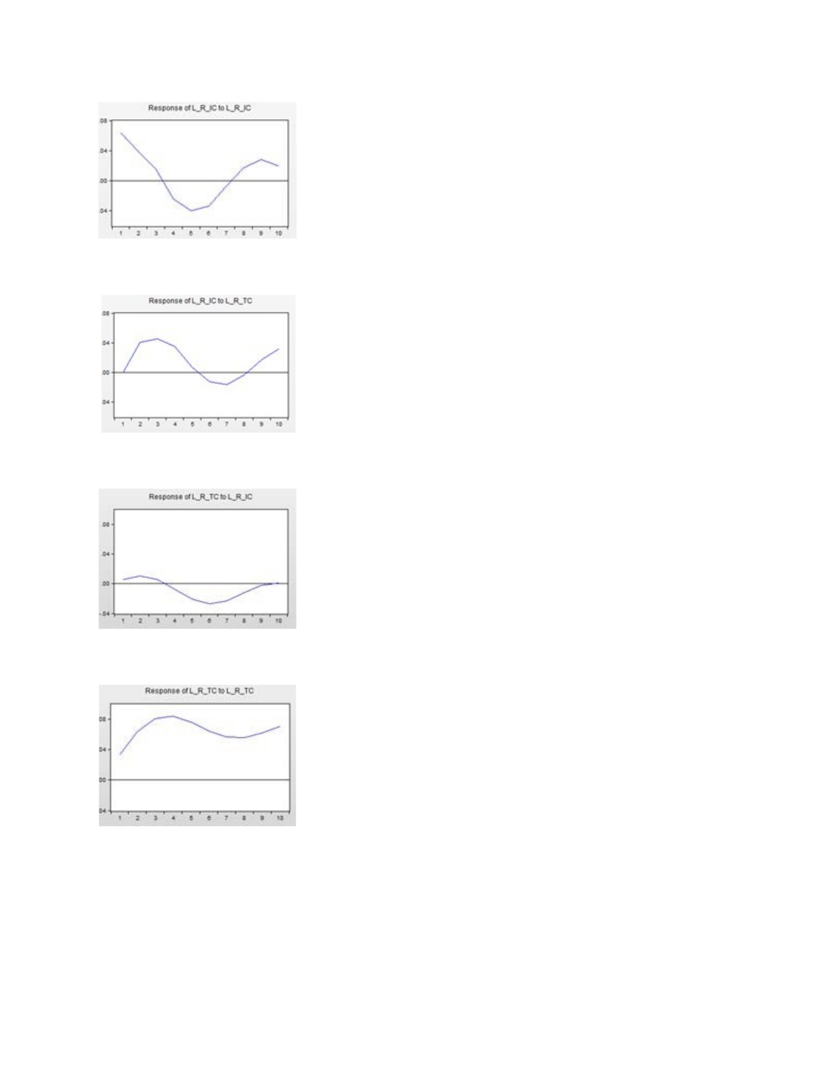
VAR systems are under-identified, so for interpretation a restriction is often implied. For this

reason, the impulse-response function was run with the Choleski decomposition which provides

a minimal set of assumptions that can be used to identify the structural model (Enders, 2010).

Panels 5-8 in Figure 4 summarize the results of the IRFs run with the Choleski decomposition.

However, notice that the patterns of the impulse response functions with the Choleski

decomposition are identical to those run with the generalized impulse response functions.

The IRFs do exhibit some limited indications of long-term equilibrium between IC and TC.

Notice in panels 1 and 2 that the response of IC to a shock of IC and TC is approaching a return

to zero. Although this return to zero is over a period longer than ten years. It takes a long time

for inventory to adjust to target levels (Feldstein et al., 1976). Likewise, TC responds to shocks

of IC with a return to equilibrium. This return to equilibrium is the only one that appears to be

completed in a ten year period, see panel 3. Shocks to TC have a permanent effect on TC, as

exhibited in panel 4. This means that there are fewer market and managerial events that can react

to offset a rise in TC. Firms can change modes or service level; however the TC must be paid in

most instances. There are some rare exceptions that allow TC to be reduced significantly or

eliminated entirely when TCs rise. For example, products that have high water content can be

shipped in concentrated form, and products that can be digitized can travel electronically. The

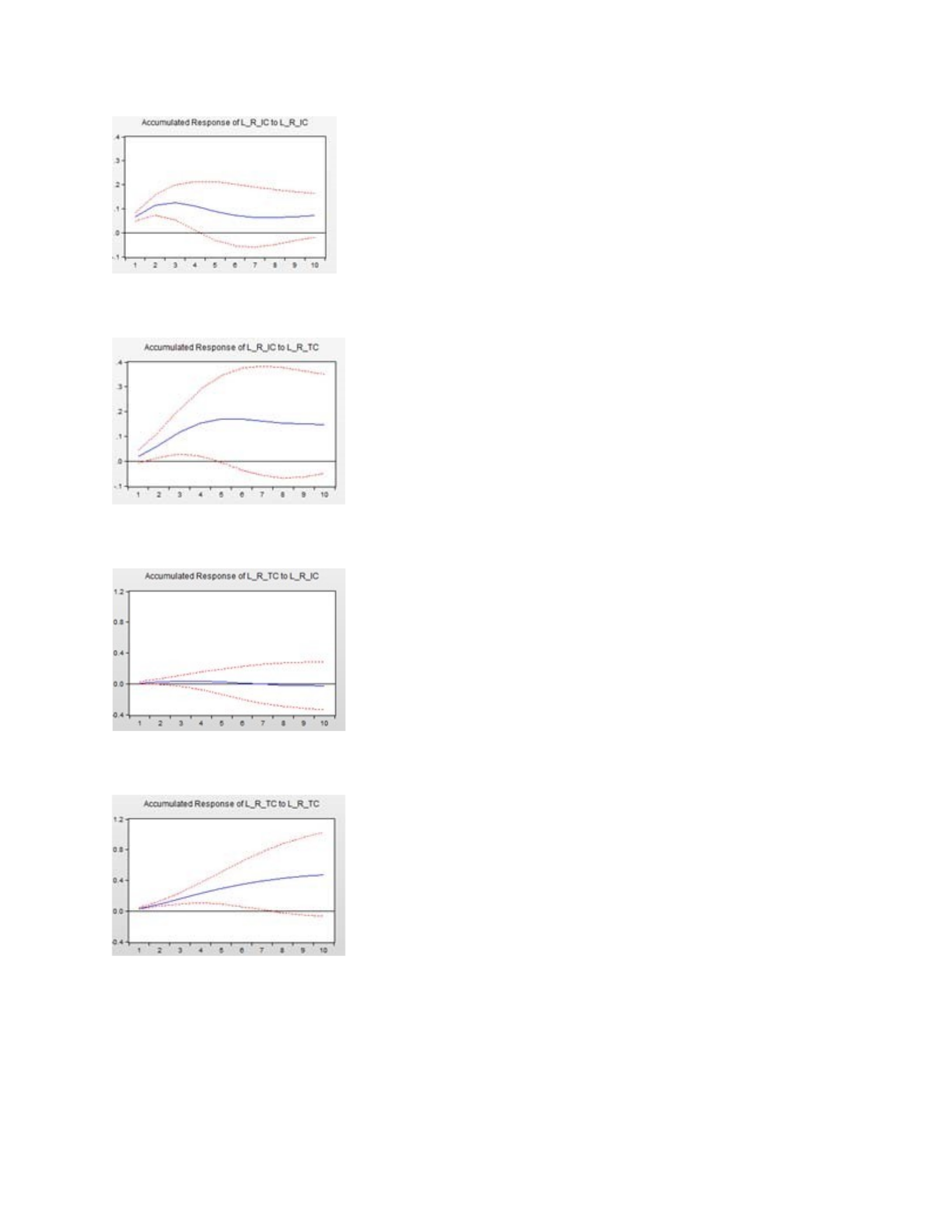
accumulated impulse response functions, as depicted in panels 9-12, provide useful information

over the course of the ten years. By examining the accumulated IRFs, observe the only shock

that returns to zero is TC in response to IC shocks, see panel 11. The response of IC seems to

find a new level near the level of the shock when responding to shocks of IC and TC as viewed

in panels 9 and 10. Panel 12 indicates that TC shocks have a permanently increasing effect. This

makes sense, when one considers that a rise in fuel cost has an ongoing and cumulative effect on

total TC.

Conclusion

IC and TC were tested for long-term and short-term equilibrium. IC and TC have been

cointegrated since transportation deregulation. This indicates that the two share a common

stochastic drift and they do share an equilibrium relationship. Over time, the model of this

equilibrium relationship shows that TCs are increasing slightly in relation to ICs.

The contribution of this analysis is extended by Granger causality tests that provide evidence of

short-term causal relationships between IC and TC. IC and TC do not share immediate,

bidirectional equilibrium. However some unidirectional, lagged variables are significant.

Changes in TC do influence firm inventory policies. The reverse relationship is not supported.

Shortterm responses to an exogenous shock may take multiple years to reciprocate. This was

expected because firms cannot change inventory policies quickly. Inelastic IC and policy can be

caused

by long-term warehousing contracts, owned real-estate, or the need to eliminate obsolete or

lowdemand inventory.

I believe that bi-directional Granger causality was not supported for several reasons. First, firms

do not always pursue lowest cost. Firms balance cost and customer service to find the best

competitive strategy that promises to give the firm a competitive advantage and increase firm

performance. Second, firms do not always calculate their costs in terms that are necessary for

this tradeoff analysis, such as stock-out cost or inventory carrying cost. Third, firms will by

nature balance lowest cost with customer service, but this usually is done by “gut feel.”

Managers learn about their business from experience and this experience and the related

decisions are not always the optimum. Furthermore, firms lack the knowledge of what the

optimum decision would have been.

Management and Policy Implications

Managers can expect IC to increase following rises in TC in the United States. A general

guideline is that IC will take about two or three years to respond to increases in TC. The other

causality direction is inconclusive, meaning IC increases do not necessarily lead to increased TC.

This study finds that transportation regulation restricted the ability of the market to follow the

natural course of self-determination from 1960 until transportation deregulation reached full

fruition in 1984. Because markets naturally migrate toward providing the most utility for the

least cost, policy makers can expect that transportation regulation similar to that with which the

United States has experience, can be expected to interfere with the optimum solution in the

marketplace, impacting both transportation and inventory carrying costs.

Figure 1: Nominal IC and Nominal TC

Figure 2: Real IC and Real TC

Figure 3: Growth rate of Real IC and Real TC

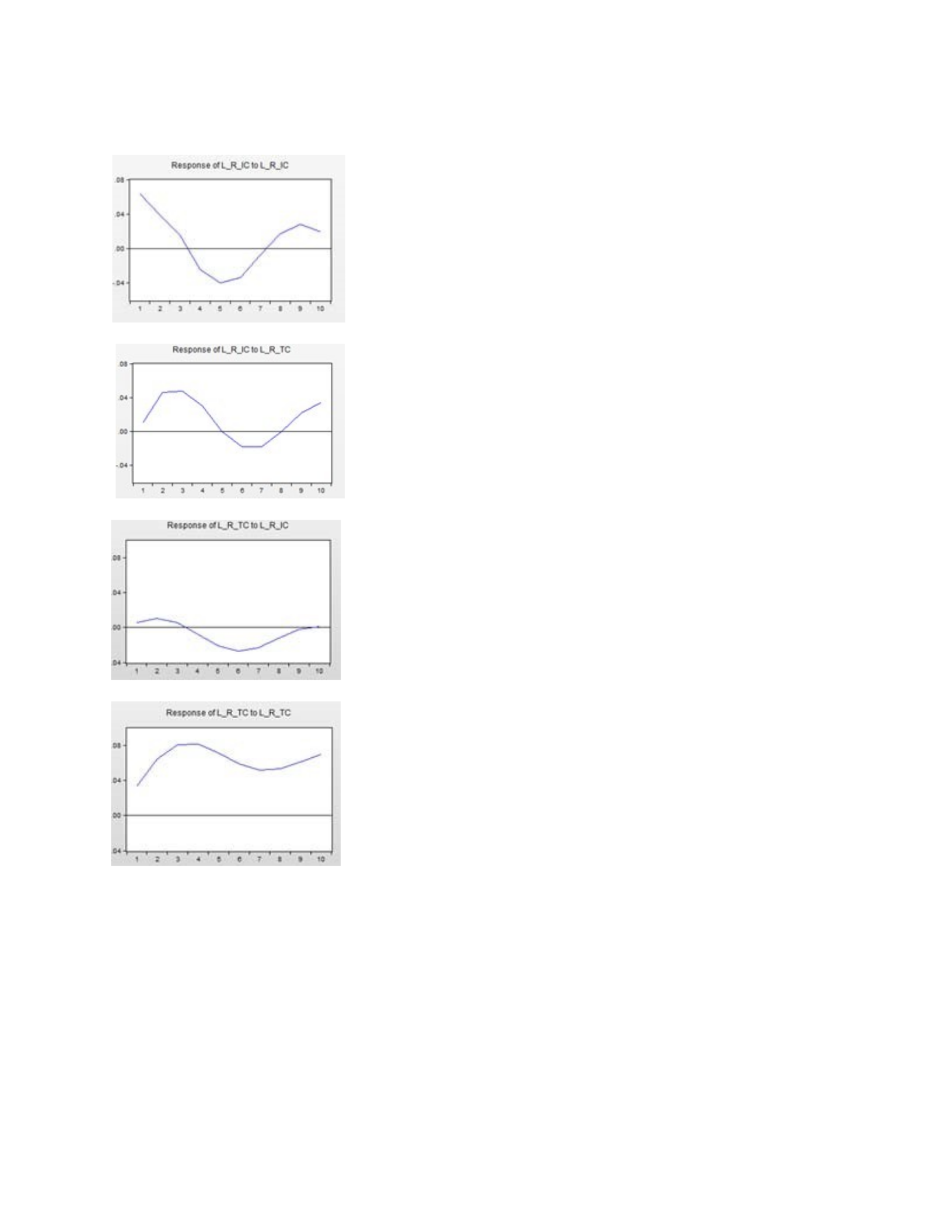
Figure 4: Impulse Response Function Results

Panel 1

Panel 2

Panel 3

Panel 4

Figure 4: Impulse Response Function Results (continued)

Panel 5

Panel 6

Panel 7

Panel 8

Figure 4: Impulse Response Function Results (continued)

Panel 9

Panel 10

Panel 11

Panel 12

Table 1: Augmented Dickey Fuller Tests for Unit Root

P-Values for ADF Tests (H0: unit root is present)

Entire Period Regulated De-Regulated

(1960-2009) (1960-1979) (1985-2009)

none α α + at none α α + at none α α + at

IC (Order) I(1) I(1) I(1) I(2) I(1) I(1) I(1) I(0) I(1)

Level 0.744 0.112 0.495 0.993 0.361 0.057 0.500 0.028 0.042

1st Diff 0.000 0.000 0.000 0.442 0.016 0.017 0.000 0.006 0.026

2nd Diff

0.000

TC (Order) I(1) I(1) I(1) I(1) I(2) I(2) I(1) I(2) I(2)

Level 0.789 0.274 0.215 0.963 0.078 0.619 0.335 0.585 0.994

1st Diff 0.002 0.019 0.047 0.017 0.094 0.146 0.206 0.862 0.914

2nd Diff 0.000 0.004 0.000 0.004 0.013

Table 2: Tau Test for Unit Root

P-Values for Tau Tests

Entire Period Regulated De-Regulated

(1960-2009) (1960-1984) (1985-2009)

H1 H2 H3 H1 H2 H3 H1 H2 H3

IC 0.054 0.125 0.230

TC 0.104 0.020 n/a

Table 3: Critical values for the tau statistics (Enders 2010)

Test Statistics 1% 5% 10%

Tau -2.62 -1.95 -1.61

Tau mu -3.58 -2.93 -2.60

Tau tau -4.15 -3.50 -3.18

Table 4: Engle Granger Cointegration Test Results

Test Statistics for ADF test of residuals from equation Ln ICt = αt + Ln TCt. (H0: unit root is

present)

Entire Period Regulated De-Regulated (1960-2009) (1960-1979) (1985-2009)

none α α + at none α α + at none α α + at

Test Statistic -1.570 -1.554 -1.380 -0.668 -0.595 -2.626 -3.303* -3.8** -4.0**

Significant at 10%*, 5% **, 1%***

Engle-Granger Critical Values (Enders 2010)

1% Critical Value -4.123

5% Critical Value -3.461

10% Critical Value -3.130

Table 5: Johansen Cointegration Test

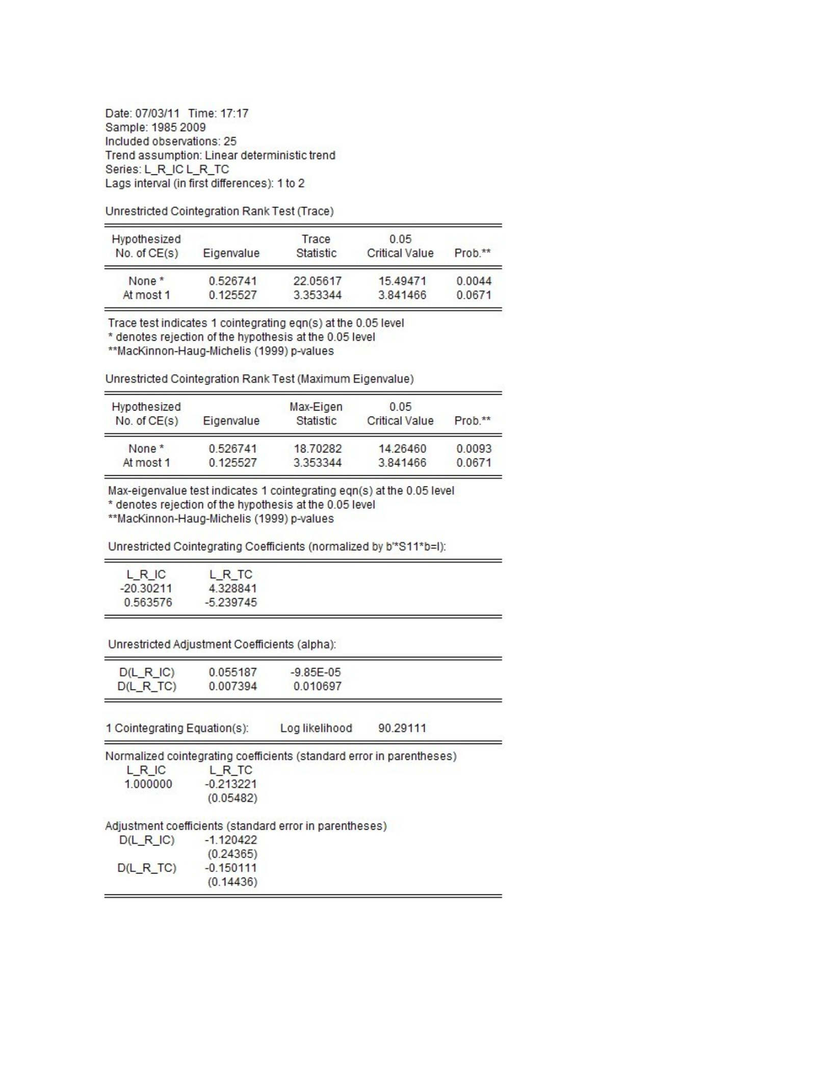
Table 6: Pairwise Granger Causality Tests (3 Lags)

Entire Period Regulated De-Regulated

(1960-2009) (1960-1979) (1980-

2009)

Obs F-Stat / Prob. F-Stat / Prob. F-Stat / Prob.

TC does not Granger Cause IC 48 1.253/0/304 2.973/ 0/065 3.319/ 0.043*

IC does not Granger Cause TC 1.088/0/365 7.304/ 0/003* 0.687/ 0.571

Evidence of Granger causality at 5% level of confidence

Table 7: VECM Comparison Statistics

AIC BIC

Δ Ln IC

One Lag -2.54 -2.34

Two Lags -2.58 -2.29

Three Lags

-2.43 -2.04

Δ Ln TC

One Lag -3.74 -3.54

Two Lags -3.63 -3.34

Three Lags -3.48 -3.09

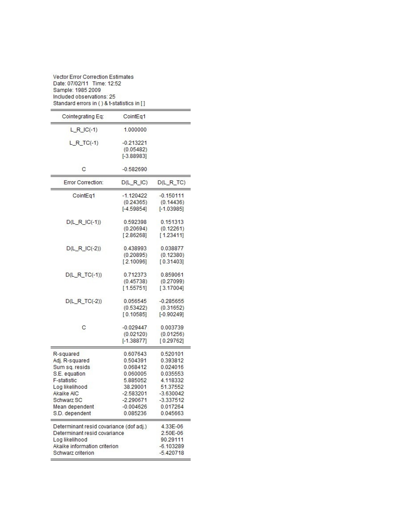
Table 8: VECM Results

References

Ballou, R. H. (1973). Business logistics management. New Jersey: Prentice-Hall.

Burns, L. D., Hall, R. W., Blumenfeld, D. E., & Daganzo, C. F. (1985). Distribution strategies

that minimize transportation and inventory costs. Operations Research, 33(3), pp. 469-490.

Defee, C. C., Williams, B., Randall, W. S., & Thomas, R. (2010). An inventory of theory in

logistics and SCM research. International Journal of Logistics Management, the, 21(3), 404-

489.

Enders, W. (2010). Applied econometric time series. United States: John Wiley & Sons, Inc.

Federal Reserve Bank of St. Louis. (2012). Retrieved August 2011, 2012, from

http://research.stlouisfed.org/fred2/

Feldstein, M., Auerbach, A., Hall, R. E., & Lovell, M. C. (1976). Inventory behavior in

durablegoods manufacturing: The target-adjustment model. Brookings Papers on Economic

Activity, 1976(2), 351-408.

Granger, C. W. J. (1988). Some recent development in a concept of causality. Journal of

Econometrics, 39(1-2, September-October), 199.

Greene, W. H. (2003). Econometric analysis (Fifth ed.). Delhi/India: Pearson Education Inc.

Lambert, D. M., Stock, J. R., & Ellram, L. (1998). Fundamentals of logistics management.

United States: McGraw-Hill Higher Education.

Langley, C. J. (1986). The evolution of the logistics concept. Journal of Business Logistics, 7(2),

pp. 1-13.

Lewis, H., Culliton, J., & Steele, J. (1956). The role of airfreight in physical distribution. Boston,

MA: The Alpine Press.

Magee, J. F. (1960). The logistics of distribution. Harvard Business Review, 38(4), p. 89.

Malley, J. R. (1990). Dynamic specification in econometric estimation. Journal of Agriculture

Economics, 42(2), 52.

Nahmias, S. (1989). Production and operations analysis. United States of America: Irwin.

Narayan, P. K., & Smyth, R. (2004). Temporal causality and the dynamics of exports, human

capital and real income in china. International Journal of Applied Economics, 1(1), 24-45.

Sheffi, Y., Eskandari, B., & Koutsopoulos, H. N. (1988). Transportation mode choice based on

total logistics costs. Journal of Business Logistics, 9(2), 137-154.

Tyworth, J. E. (1992). Modeling transportation-inventory trade-offs in a stochastic setting.

Journal of Business Logistics, (2), 97.

Venturini, F. (2009). The long-run impact of ICT. Empirical Economics, 37(3), 497-515.

Wilson, R., & Delaney, R. V. (2001). 12th annual state of logistics report. ( No. June 4).

Washington DC: National Press Club.

CHAPTER 3 (ESSAY 2): The Relationship between Inventory and Transportation: An

Inventory-Theoretic Study with Firm-Level Inventory and Transportation Cost

Abstract

This essay tests the relationship between inventory cost (IC) and transportation cost (TC) at the

firm level based on an inventory-theoretic perspective. Inventory theory posits that firms will

trade off IC and TC to minimize the sum of their cost (Baumol & Vinod, 1970). Studies in

macroeconomics (Swanson, 2012) indicate tradeoff properties of IC and TC. Firm-level IC and

TC and their relationship have not been tested. This essay tests this theory.

Panel data involving transportation and inventory expenditures of 41 firms and 22 quarters from

2006 through 2011 was collected as the sample for this study. A model was specified to predict

firm inventory with independent variables suggested from inventory-theoretic literature. A

contribution was made by including TC in the inventory model. Firms do trade off IC and TC in

the course of logistics management. Also found is a negative relationship between a one-period

lag of TC and inventory. TC is shown to be a useful variable for predicting inventory.

Introduction

One type of business cost, total logistics cost (TLC), often exceeds 25% of sales (Ballou, 2000;

Stock, Lambert, & Lambert, 1987). Technology and human resources applied to improving

supply chain performance have never been higher (Fisher, 1997). Accordingly, logistics

expenditures are highly scrutinized by firm managers.

The theory of TLC management posits that firms will seek to minimize total logistics cost

(Lewis et al., 1956) by managing key logistics functions as a system (Lambert et al., 1998).

Furthermore, firms will trade off key logistics cost (Bowersox, 2007); two of which are IC and

TC, to minimize TLC.

This essay shows first that there exists a predictable relationship between IC and TC, and second

that the relationship can be measured. These demonstrations provide valuable contributions that

increase our understanding of inventory and transportation which can be used to enhance

management performance. For example, if a firm expects TCs to increase 5% in the future, then

one could expect inventory expenditure and its associated costs to increase as well by a

measurable amount. With this knowledge, firms can optimize their mix of transportation and

inventory cost more quickly in response to exogenous cost increases and in response to

competitor strategies. This allows the firm to be more proactive in meeting a TLC objective.

Theory and anecdotal evidence suggest that firm management does trade off expenditures of

inventory and transportation to fit its strategy and to adjust to external factors. For example, if

TC falls, firms may choose to decrease cycle stock, ship more frequently, and thus reduce their

inventory carrying costs. Similarly, if TC rises, firms may choose to take advantage of

transportation economies of scale and volume shipping incentives that are provided by carriers

and suppliers to lower their transportation expenditures (Simchi-Levi, Kaminski, & and Simchi-

Levi, 2003). The previously unconfirmed, conventional knowledge suggested this would cause

IC to rise. The first essay of this dissertation (Swanson, 2012) finds supporting empirical

evidence that IC and TC share a long term relationship when this relationship was examined with

aggregated costs in the United States. However, there has been little empirical research on

management behavior regarding the tradeoff potential of IC and TC. It is important and

interesting to extend research on management behavior because macroeconomic and firm-level

results are often different (Pilat, 2004). An empirical analysis of firm-level data may provide

different results than the macroeconomic results and could benefit management.

Although theory posits firms balance IC and TC and pursue minimum TLC, there are reasons

that firms may not choose to balance IC and TC and thus pursue a lowest total cost. Firms may

choose to pursue alternate transportation or inventory service strategies (Porter, 1980), may be

bound by contractual agreements (Phillips, 1991), may suffer from lack of information or the

accurate interpretation of it (Ferguson, 2001; Lieberman, Helper, & Demeester, 1999), or they

may have inferior or inappropriate resources (Barney, 1991) or capabilities (Teece, Gary, & Amy,

1997). Firms may choose to seek lowest cost, but immediate cost adjustment can be difficult in

the near term. Regarding TC, firms may have private fleet investments which are difficult to

divest (Maltz, 1993). Regarding IC, firms also may have service-level commitments with

customers or may have difficulty liquidating large amounts of inventory (Feldstein et al., 1976).

Additionally, many logistics cost variables are not within the control of management, such as fuel

prices, interest rates, inflation (Chen, Frank, & Wu, 2005) and consumer preferences.

The question remains whether firms show evidence of trading off these key logistics costs or if it

is merely a macroeconomic artifact. The objective of this essay is to analyze whether the

insights from the macroeconomic level of equilibrium between IC and TC are consistent when

analyzing the IC and TC at the firm level using inventory theory.

This essay begins with a review of two streams of related literature. The first of which explores

the theoretical relationship of IC and TC. The second stream is inventory theory. From this

theoretical foundation, this essay develops and hypothesizes the relationship between IC and TC

at the firm level. At the same time, this essay tests TC as a predictor of firm inventory.

Following hypothesis development, this essay describes the data sampling process, the

descriptive statistics, and introduces a model. This is followed with results and discussion. The

essay ends with conclusions, management implications, limitations, and future research

possibilities.

Literature Review

Theoretical Relationship of Inventory and Transportation Cost

Economic theory has been commonly applied to the inventory-theoretic literature supporting that

tradeoffs exist between IC and TC (Blinder & Maccini, 1991). Theory suggests that when firms

are operating at the most efficient TLC that inventory holding cost equals inventory ordering

(transportation) cost, IC = TC (Baumol & Vinod, 1970; Harris, 1913). Suppose firms experience

an increase in inventory carrying cost, such as an interest rate increase. The above theory

suggests that firms will spend more on ordering cost (transportation) for more frequent deliveries

and lower inventory carrying cost because IC > TC. Likewise, if TC increase, such as by an

increase in fuel prices, the balance is upset again. This time TC > IC so firms react by spending

less on TC, which might involve, for example, less frequent deliveries. Less frequent deliveries

lead to larger inventories, ceteris paribus, which also act to return IC = TC.

Logistics cost tradeoffs, including that of IC and TC, have been theorized for a century beginning

with the development of the basic economic order quantity (EOQ) model (Camp, 1922;

Hendricks & Singhal, 2003) and production lot size model (Taft, 1918). Initially, the EOQ

model and theory focused on inventory carrying cost and ordering cost. However, in the early

1970s comprehensive comparisons of freight options considered the inventory holding cost in

association with transportation (Zeng & Rossetti, 2003). The basic model was enriched to

explain more of the relationships between logistics variables including the expansion of ordering

cost to include TC (Chen, Frank, & Wu, 2007), additional transport-related variables (Buffa &

Reynolds, 1979), safety stock formulations (Stenger et al., 1977), enhanced stock-out modeling

(Constable & Whybark, 1978) and more accurate TC (Langley, 1980). See (Sandlin, 2010) for

an extensive literature review.

The question of how to determine logistics cost has been an important and prolific source of

literature that provides information accounting for IC and TC. Maltz et al. provide a logistics

cost categorization framework. (Maltz & Ellram, 1997) . Another costing approach was studied

in a dissertation by Knipper (Knipper, 2011). Studies on the total cost approach (Ellram, 1994)

and total profit approach (Poist, 1974) have been applied. Activity-based costing is prevalent in

logistics costing (Pirttila & Hautaniemi, 1995). This paper, however, concentrates on the

relationship of IC and TC and does not delve into the issues of costing methods.

Further support for the tradeoff potential of key logistics variables comes from the concept of

TLC management which was a founding pillar of the discipline of business logistics management

in the 1950s (Bowersox, 1969; Bowersox, 2007; Langley, 1986; Lewis et al., 1956; Magee,

1960). Scholars warned about indiscriminate changes in one functional area of the firm without

assessing the potential changes to another related functional area (Magee, 1960). Areas such as

warehousing, transportation, and logistics administration had costs that were interrelated. For

example, minimizing purchase cost by pursuing economies of scale can adversely affect

warehouse storage cost and capacity. Because of the importance of integrated logistics functions

and TLC management, university programs in business logistics have taught tradeoff principles

since the first college class at Michigan State University in 1958 and the first logistics

management textbook (Smykay et al., 1961). Since this beginning, there are now over 65

universities that offer a degree or concentration in business logistics or supply chain management

and many universities offer doctoral education (Ozment & Keller, 2011). All of these programs

are based on the principles of functional area tradeoff inside the company (Magee, 1960) and

between supply chain partners (Cooper, Lambert, & Pagh, 1997). The discipline continues to

grow.

There has not been an analysis of secondary data to study the tradeoff of IC and TC. Studies

primarily focus on either inventory or transportation (Mason, Mauricio Ribera, Farris, & Kirk,

2003). This essay is relevant because if TC is related to decisions about inventory, then its use in

models that predict inventory can be added to the inventory-theoretic literature. That literature is

summarized next.

Inventory-Theoretic Literature

The study of inventory is important because it is directly related to firm and economic

performance (Feldstein et al., 1976). High levels of inventory cause lower performance or it is

perceived to yield lower performance (Chen et al., 2005; Chen et al., 2007; Lai, 2006). Retailers

are less likely to go bankrupt (Randall, Netessine, & Rudi, 2005) if they operate in accordance

with classical inventory models.

The classical inventory models, including the EOQ, are derived at the product level and intended

to be used for stock-keeping unit (SKU) level analysis and optimization. Rumyantsev et al.

extend these theories, testing inventory-theoretic variables on inventory-level data and show that

these product-based models can apply to aggregated levels of SKUs (Rumyantsev & Netessine,

2007). Rumyantsev et al. go on to show that aggregate firm inventory is related to demand

uncertainty, lead times, margins and economies of scale similar to single-product inventory.

The classic economic lot size model (Harris, 1913) is a simple framework that illustrates the

trade-offs between ordering and inventory holding costs, without the effect of demand

uncertainty. The EOQ theory assumes that firms will seek to minimize their TLC. TCs are an

example of ordering cost. Holding cost includes maintenance cost such as taxes and insurance,

obsolescence, and opportunity cost (Lambert et al., 1998). These logistics costs are a sum of

holding cost (H (Q/2)) and TC (K (D/Q)). Where: H = annual holding cost, Q = optimal order

quantity, K = transportation cost per order, and D = annual demand.

Since demand is uncertain, the sales forecast is critical for the determination of what and when to

order (Simchi-Levi et al., 2003). If a firm forecasts too much demand, it is left with costly

inventory. If the firm forecast is less than demand, it loses sales. Demand is primarily

stochastic, so it is estimated using forecasting, with uncertainty often measured by the standard

deviation (Simchi-Levi et al., 2003). The impact of lost sales is largely unknown because lost

sales are difficult to measure.

Average lead time and uncertainty are included in the inventory-theoretic literature. When

studying the effects of lead time and lead time uncertainty on inventory values, the TC of the

firm is indirectly studied, because, generally shorter and less certain lead times are more

expensive. Yet theory suggests that TC should be measured directly because of its tradeoff

relationship with inventory (Baumol & Vinod, 1970; Swanson, 2012).

Empirical inventory research has revealed information regarding the relationship of inventory

levels and key variables. Studies have shown that firms hold more inventory when they have

higher sales demand and higher demand uncertainty (Rumyantsev & Netessine, 2007; Zinn,

Levy, & Bowersox, 1989), longer lead times, (Evers, 1999; Rumyantsev & Netessine, 2007),

lower capital cost, higher gross margins (Gaur, Fisher, & Raman, 2005), and higher stock-out

cost (Constable & Whybark, 1978). Other studies have also shown that firms carry more

inventory when the stock market puts a premium on inventory (Lai, 2006), when product variety

increases (Fisher & Ittner, 1999), when information systems are inadequate (Ferguson, 2001), or

a firm may increase inventory simply because they don’t know it is costly (Timme, 2003).

Justin-time (JIT) inventory operations reduce inventory levels for manufacturers but not in other

sectors of the supply chain (Rajagopalan & Malhotra, 2001). All of this empirical research can

be summarized in three reasons firms hold inventory: to satisfy demand during lead time, to

protect against uncertainty in lead time and demand, and to balance annual inventory holding

cost and annual supply cost (Simchi-Levi et al., 2003). Transportation has an impact on all of

these reasons that firms hold inventory.

Some limitations of classic inventory models include that they do not account for factors such as

competition, business cycles, industry dynamics, and do not represent some other decisions that

could be handled endogenously by the firm such as pricing and product variety (Rumyantsev &

Netessine, 2007). Even many simple heuristics that are used for decision making can outperform

the classic EOQ approach; for an overview of these heuristics see Silver et al. (Silver, Pyke, &

Peterson, 1998).

Hypothesis Development

Economists have tracked aggregate IC and TC in the United States since 1960 (Wilson &

Delaney, 2001). This data suggests that TLC has decreased as a measure of GDP (Langley,

1986) and the behavior of aggregate IC and TC in times of GDP expansion and contraction is

different (Wilson & Delaney, 2001). The first empirical test of the relationship of IC and TC

(Swanson, 2012) demonstrated that IC and TC are cointegrated, and that they share a long-term

relationship at the macroeconomic level. This is consistent with inventory theory which suggests

that firms trade these costs to achieve lowest TLC (Swenseth & Godfrey, 2002; Tyworth, 1991).

Just as the theory was tested on macroeconomic data, the behavior of firm-level IC and TC

should also be empirically tested.

Firms hold inventory for several reasons including demand uncertainty, transportation

uncertainty, and because production does not perfectly coincide with customer demand

(SimchiLevi et al., 2003). In previous research, scholars have verified drivers of inventory

holdings (Fisher & Ittner, 1999; Gaur et al., 2005; Rajagopalan & Malhotra, 2001). This essay

reproduces the drivers of inventory suggested by extant literature as a foundation, and then tests

the model with the addition of TC.

Rumyantsev and Netessine address two crucial aspects of firm-level inventory analysis: time and

space aggregation and the difference between the prescriptive inventory models and the

descriptive parameters seen commonly in practice (Rumyantsev & Netessine, 2007). These

authors also test multiple hypotheses related to whether inventory models that are designed for

use at the product level can also be useful for firm-level analysis. Similar to this previous

research, this essay must overcome two challenges. First, several of the inventory variables in

this study come from classical inventory models and those models are designed for use at the

product level. This poses complications (Rajagopalan & Malhotra, 2001) for studies done at the

aggregate level (Gaur et al., 2005). However, there is precedence and support for the validity of

classical inventory models to be used on aggregate data (Rumyantsev & Netessine, 2007).

Secondly, this study is done with accounting data that managers use as the basis for inventory

management decisions. Similar to Gaur et al. (Gaur et al., 2005), this study must overcome the

discrepancy between observation of the data and the behavior of the managers after they observe,

interpret, and respond to the data. Firm behavior results from the relative relationships of the

variables, including transportation expenditures, inventory, sales, cost of goods sold (COGS),

interest rates, and accounting practices (Rajagopalan & Malhotra, 2001).

Inventory theory suggests that IC and TC share an equilibrium relationship and that firms will

tradeoff IC and TC (Tyworth, 1991). Yet, TC is missing from the empirical models in the extant

literature. Studies have shown that firms increase inventory when they have higher sales

demand, longer lead times, higher gross margins, lower capital cost, higher stock-out cost, and

higher demand uncertainty (Rumyantsev & Netessine, 2007). In these models, TC is partially

reflected in the variables of lead times and higher lead time uncertainty. However, theory

suggests that TC should be measured directly for the purpose of predicting inventory (Baumol &

Vinod, 1970).

The classic EOQ model explains that firms optimize TLC by adjusting the amounts they spend

on inventory and transportation to find the right mix for the market which will yield the lowest

TLC (Fisher, 1997; Harris, 1913). Subsequent research supports that firms will balance their

transportation and inventory carrying cost to achieve the lowest TLC (Campbell, 1990; Ellram &

Siferd, 1998). EOQ theory (Harris, 1913) defines the lowest total cost to be achieved when

inventory carrying cost equals ordering and TC. Therefore, if a firm must spend more on one

cost (IC or TC), they should spend more on the other as well in an attempt to keep TLC at a

minimum.

The inventory theory of the EOQ is not without controversy (Silver et al., 1998; Speranza &

Ukovich, 1994). Practitioners complain about the model’s simplicity and that in most instances

inventory is managed at an aggregate level instead of at the product level (Bishop, 1979). In the

long-term, firms may not always pursue the lowest cost (Porter, 1980). A mathematical

programming model of the cost and service tradeoff is available (Das & Tyagi, 1997). Firm

capabilities may match strategies other than lowest cost particularly well and accordingly firms

may elect to pay more to provide a premium service (Lynch, Keller, & Ozment, 2000).

Inventory theory suggests that firms will minimize TLC when a firm’s inventory holding cost

equals its ordering cost (Harris, 1913). Since ordering cost includes TC (Chopra & Meindl,

2004), a positive relationship between IC and TC is expected. Theory suggests that if a firm

increases inventory they must have a corresponding rise in TC in order for the firm to rest at its

new minimum TLC. See Figure 1. This leads to the following hypothesis.

Hypothesis: Transportation cost is positively related to inventory.

Data

Sample Selection

The sample includes weekly TC from September 2006 through March 2011 for 126 firms.

Weekly TCs were summed by quarter so that there was a match between TC and the quarterly

inventory levels. Quarters that included more than two vacant weeks were deleted because there

was insufficient data to track the quarterly total. In some cases the first week of data provided by

the firm was considerably less than the following weeks. In such cases it was possible that a firm

began tallying TC mid-week, so these partial weeks were removed from the database.

Firms without at least three years of data were deleted to allow study of time effects. This data

cleanse process left 50 firms with at least 12 quarters of TC.

Inventory and other company-related variables were extracted from the Standard and Poor’s

Compustat database. Three firms did not provide quarterly inventory data and so they were

removed from the sample. There were also five firms which could not be unambiguously linked

to the transportation data. This was usually due to mergers, divestment, or multiple company

divisions that made the matching unclear. These five firms were removed from the sample.

Quarterly data was chosen instead of annual data because this provided substantially more data

observations, which is desirable for analyzing inventories due to their highly dynamic properties

(Carpenter, Fazzari, Petersen, Friedman, & Kashyap, 1994). Had annual data been used, three

more companies could be included in this analysis; however, this would have been relatively

small because, by using quarterly data, observations increased from 160 to 564. After removing

firms for inventory data issues the sample was left with 42 firms. When calculating the

inventory variables for the model, additional observations were sacrificed. For example,

(Uncertaintyit) is measured by using the forecast error from the previous three quarters.

Calculating some inventory variables reduced total observations in my sample to 322 quarters.

Descriptive Statistics

Descriptive statistics and pairwise correlations are summarized in Table 1 and Table 2. The mean

IC is about one-third of TC, a sizeable difference. This is consistent with our expectations

(Wilson & Delaney, 2001). Also, the standard deviations are all lower than the mean which

indicate low data uncertainty.

From examination of the descriptive statistics, it was decided to keep the data in its purest form.

Taking the natural logarithm was unnecessary because the data wasn’t highly skewed. The

histogram of the dependent variable (Inventoryit) demonstrated that the data follows a normal

distribution.

The firms in this sample represent 18 industry groups as measured by the first three North

American Industry Classification System (NAICS) numbers. They represent 10 industry groups

if measured by the first two NAICS numbers. Twenty-five percent of the NAICS classifications

in the sample data come from retailers and seventy-five percent come from suppliers. Detailed

NAICS representations are provided in Table 2.

Methodology

Model Specification

OLS assumptions of homoscedasticity and independence are often not met when dealing with

panel data (Greene, 2003). Therefore tests for homoscedasticity and autocorrelation of the errors

were implemented prior to selecting the appropriate estimation procedure.

Residuals from the model were plotted across time and examined for evidence of

heteroscedasticity. The test showed minor evidence of heteroscedasticity and since the structure

is not known, the use of OLS with White robust standard errors is recommended to control for

the expanding variances (Kennedy, 2008).

Residuals from the model were examined for evidence of autocorrelation with the DurbinWatson

statistic (2.44 ). Since the statistic is not near the values of 1 or 4, this indicates no abnormal

evidence of serial correlation and OLS will provide consistent and robust results.

Inventory theory states that a firm’s inventory level is a function of several different variables.

Foremost among these are sales, sales forecast, the order quantity (Camp, 1922; Gaur et al.,

2005; Harris, 1913), safety stock level, sales surprise (Gaur et al., 2005), and inventory

accounting methods (Carpenter et al., 1994; Rumyantsev & Netessine, 2007). Extant literature

suggests Equation 1.

Inv = f (Q, SS, SSP, S, SF, A) (1)

Where Q is order quantity, SS is safety stock level, SSP is sales surprise, S is sales, SF is sales

forecast, and A is used to designate accounting methods.

The order quantity is a function of the expected demand, and the costs of holding inventory,

ordering, and stock-out costs. Safety stock is a function of lead times, expected sales, the degree

of demand and lead time uncertainty, and the safety factor (k). The safety factor is determined

by the managers as an acceptable level of the probability of a stock-out. Empirically this has

been measured by minimizing the sum of inventory holding and stock-out costs (Carpenter et al.,

1994; Rumyantsev & Netessine, 2007). Combining these equations suggests Equation 2.

Inv = f ( S, SF, U, S%, HC, OC, SOC, LT, A). (2)

Where S = Sales, SF = Sales forecast, U = demand lead time uncertainty, S% = safety factor, HC

= holding cost, OC = ordering cost, SOC = stock-out cost, LT = lead time, and A = inventory

accounting method.

This model has been used to empirically estimate firm-level inventory (Hofer & Waller, 2012).

The variables in Equation 2 can be estimated from easily attained financial data with the

exception of order placement costs. Hofer et al. (Hofer & Waller, 2012) justify the elimination of

this variable because a prior empirical study that has measured order costs was not found, and the

widespread use of EDI has reduced the costs associated with placing and processing orders

(Avery, 1998; Hofer & Waller, 2012; W. Min & Pheng, 2006a; W. Min & Pheng, 2006b). In this

model, TC is used for partial representation of total order placement cost. This will allow for at

least some portion of the ordering costs to be accounted.

Model Variables and Measurement

The dependent variable (Inventoryit) for this study is total firm-level inventory (i) in period (t)

and is measured in U.S. dollars. Prior research supports use of absolute inventory values

(Rumyantsev & Netessine, 2007).

Firms use expected demand (SalesForecastit) as the basis for their replenishment decisions. In

line with previous research (Hofer & Waller, 2012), annual sales for each firm and time period

can be forecast by , where the average growth rate from the previous two

years () is defined as follows.

/ / /

2 (3)

Firms make decisions based on expected demand, but also they base their decision on the

accuracy of their forecast during the previous period. This is determined by the net of expected

demand and actual demand. If firms under forecast their demand, the magnitude of inventory on

hand at the end of the quarter is lower. If firms over forecast their demand, the magnitude of

inventory on hand at the end of the quarter is higher. Sales surprise (SSit) is the variable that

measures the difference between expected and actual demand (Gaur et al., 2005). A procedure

from prior research was used to measure this variable (Hofer & Waller, 2012; Rumyantsev &

Netessine, 2007).

Forecast uncertainty (Uncertaintyit) can be estimated by the magnitude of variability in forecast

errors. It is commonly measured as the coefficient of variation of forecast errors (Watson, 1987),

or the ratio of the standard deviation of forecast errors over the previous three years and the

current period forecast (Hofer & Waller, 2012).

, , / (4)

The capital cost of holding inventory is a function of the capital interest rate (Timme, 2003).

This represents both the opportunity cost of internally financing inventory and the cost to borrow

money to finance inventory. The cost of capital (CostofCapitalit) can be estimated by dividing

the firm’s interest expense by total debt.

(5)

A measurement of the lead time for physical distribution is difficult to attain. However, it is

believed that the payment of goods is highly correlated with the shipment of goods. Therefore,

in line with previous research (Hausman, 2002; Rumyantsev & Netessine, 2007) the cash

conversion cycle is used as a proxy variable to represent firm lead times (LeadTimeit).

Where accounts payable is denoted as AP and cost of goods sold is denoted as COGS.

The measure of stock-out cost (StockoutCostit) is approximated by gross profit margin because it

is in proportion with the foregone profit (Dulaney & Waller, 2002).

Inventory data is collected from balance sheet filings of publicly traded companies. The

accounting principles of inventory costing have an effect on the inventory value used in this

model. Specifically last-in-first-out (LIFO), first-in-first-out (FIFO), average cost (AC), or a

combination (MC) of these accounting measures can be used to determine book value of

inventory. LIFO inventory means that the purchase price of the oldest products determine the

value; FIFO valuation means the latest purchase prices determine the inventory value; AC

provides an average value calculated from all purchases. In times of purchase price inflation or

TC changes, these values can be substantially different. Therefore, inventory accounting

methods are measured with dummy variables (FIFOit, LIFOit , AveCostit, and MixCostit).

Ordering cost is composed of the item cost and the handling (including transportation) cost

(Simchi-Levi et al., 2003). For this essay we use quarterly TC (TransCostit) as a variable to

represent ordering cost. TC includes the payments made to carriers. This does not include cost

of private fleets that are maintained by some of the companies in the dataset.

The resulting empirical estimation equation is:

The model (Equation 3) is implemented with cross-sectional or firm fixed effects. This provided

control for the alternative inventory accounting methods among other unknown fixed effects.

Thus, the inventory valuation dummy variables were unnecessary and omitted.

Results

The results from testing this model using the panel data set and linear regression appear in Table

3. The model’s F statistic (F=1.56) is statistically significant (p = 0.05), and the overall Rsquared

statistic is 0.20, which indicates that the model explains approximately 20 percent of the

variability in the dependent variable (Inventoryit).

The hypothesis, that inventory level is positively associated with TC, is not supported because

the sign on (TransCost(-1)) is negative indicating an inverse relationship between IC and TC.

However, (TransCost(-1)) is a significant variable for the prediction of inventory, and we

conclude that firms do trade off IC and TC. This conclusion provides information about the

association of IC and TC. The association doesn’t indicate causality because of the difficulty

making specific causal conclusions without the specific population data that is used by inventory

decision makers.

Discussion

Management tradeoff of inventory and transportation cost

This essay demonstrates that firms do trade off IC and TC in the process of managing the

logistics operations of their firms (p=0.0158). When a firm experiences a TC increase, the first

reaction of managers is not to spend more on inventory rather, managers will attempt to lower

costs that can offset the TC increase (Lambert et al., 1998). For example, if fuel prices increase,

they can counter this increase by shipping on longer trailers or delivering less often. A spike in

TC may also raise the priority of changing inventory policies that could reduce the cost of

inventory and help to offset the rise in TC. Some examples of such inventory policy changes

include consolidating warehouses or urging suppliers to accept more of the inventory cost burden

with projects such as vendor managed inventory (Waller, Johnson, & Davis, 1999) or just-intime

(JIT) manufacturing.

The negative relationship between inventory and transportation

A positive relationship was not found between IC and TC. TC (lagged) has a negative influence

on inventory (p=0.0158), so firms are spending too much on logistics cost in the short-term. This

conclusion is contrary to our hypothesized result from inventory theory. Theory suggests that an

increase in TC should result in policy changes by the firm that have a net increase in IC so that

TLC can be minimized, such as an increase in the order quantity.

Explanation for the negative relationship between IC and TC

This essay suggests five possible reasons for the negative relationship between TC and inventory.

First, firms do not necessarily have equal control over changing IC and TC because of

operational, contractual, or environmental reasons. Second, budget constraints may limit firm

options. Third, irrational behavior may be a possible explanation. Fourth, the relationship

between IC and TC may not be purely unidirectional. Fifth, management may be driven by

other goals rather than merely lowest cost.

Firms do not necessarily have equal control over IC and TC changes. Consequently, the

adjustments to IC and TC are not necessarily consistent or predictable in the short-term.

Regarding IC, the firm can make inventory policy changes to reduce IC, such as implementing

smaller manufacturing lots (Silver et al., 1998) or consolidating warehouses (Zinn et al., 1989).

However, the firm will still have to pay the higher interest rates. Regarding TC changes, the firm

can alter policy such as shipping on longer trailers or negotiating a lower priced contract.

However, they still have to pay the higher fuel cost. After the firm makes adjustments, the

shortterm TLC may rest higher or lower than the starting point. It depends on the mix of TC and

IC changes that are inherent in the policies that firms pursue.

Firm management often has to make operational decisions based budget constraints. For

example, when interest rates rise, then IC increases; and theory suggests ordering smaller

quantities and shipping more often. However, because of short-term budgetary constraints,

managers may be unable to increase transportation expenditure or may be unable to forego lower

item prices that were based on a larger order quantity.

Another possible explanation is irrational behavior. This could originate from lack of skill, lack

of information, or poor decisions. Managing a business by minimizing TLC is difficult.

Managers may lack skills in some functional areas of logistics which limit their ability to meet

lowest TLC. Firms may lack the knowledge or information systems that are required to

summarize complex business operations. Managers may make decisions that are less than the

optimum. Irrational behavior may take many forms, which in turn, might explain the negative

short-term relationship between IC and TC.

The short-term behavior of these variables is sporadic and not purely unidirectional. A positive

relationship is not always found because firms are adjusting to their new market circumstances

which take several iterations of fluctuation (Feldstein et al., 1976). Even though a positive

relationship between IC and TC, suggested by inventory theory, is not supported in the shortterm,

a positive relationship could be found in the long-term. It is likely that firms require multiple

quarters to reach equilibrium; however, in each quarter of observation, individual firms are at

different stages in the process. Some are in the first quarter of responding to a TC shock, other

firms are in the 10th quarter of response. The different stages of reaction (lags) represented by

multiple firms is averaged. Models with additional and alternative lags were tested.

However, the model with the best fit was found when observing the immediate, one-period lag of

TC. When observing additional lags, the variables become insignificant. The initial reaction to a

rise in transportation cost (TransportationCost(-1)) is an immediate reduction in inventory

(Inventoryit). The negative coefficient on IC indicates that, in the near term, the firm brings IC

cost down to offset the increase in TC.

Management does not always pursue lowest cost in the short-term. Premium service is often a

management goal and is seldom the lowest cost option. Also, management may pursue lowest

cost with a longer term perspective. For example, when sourcing additional tractor equipment,

management may decide that it is less expensive to buy newer, more expensive tractors than to

save money on the purchase price, but pay more during the ensuing months with higher

maintenance costs and lower fuel economy.

Conclusion

This study draws on inventory theory to test whether firms trade off IC and TC. Specifically, it

argues that the inventory-theoretic literature supports that firms manage inventory and

transportation expenditures in concert, always monitoring the effect on one to changes in the

other. Analysis with a large sample of firms provides suitable empirical support for testing the

relationship between IC and TC. This research provides evidence that managers do trade off IC

and TC in an effort to effectively manage their firms.

The essay concludes that managers will trade off IC and TC in an attempt to reduce total logistics

cost. However, the changes to IC and TC are dynamic. The first period of adjustment

demonstrates a negative relationship, meaning that if a firm’s TCs increase, then management

decreases IC in the next period to offset the TC increase. The next several quarters are not

statistically significant and the association in subsequent periods cannot be determined

unambiguously.

This is the first research that could be found that empirically tests management behavior related

to IC and TC trade off. This research advances the inventory-theoretic literature by

demonstrating empirical support for the inclusion of TC as a variable for the prediction of firm

inventory. The most important practical implications from this study include enhanced

information and support for managers to predict and react to IC changes more effectively and

efficiently.

Management Implications

In practice, most firms have an organizational structure that divides transportation and inventory

departments and they operate separately. Through daily activities, inventory planners forecast,

source, store, and ultimately serve the fulfillment of customer requests. Transportation planners,

likewise, plan their present and future transportation requirements based on forecasts of

consumer demand. Cross-functional management collaboration between logistic functions

appears to be rare in practice (Ellinger, 2000). These functions usually aren’t managed

collectively until the senior management level, where a firm may have a vice-president of

operations who presides over both transportation and inventory divisions. Such an

organizational structure impedes interaction between lower and mid-level managers that make

transportation and inventory decisions. However, this study finds evidence that costs incurred in

the transportation division of the company will have effects on inventory in the following

quarter. This information can be used to suggest alternate organization structures and

management behavior to better manage total logistics cost.

Future Research

The effect of customer service strategy on the behavior of IC and TC

The pursuit of low cost does not occur in a vacuum. Firms routinely balance cost with customer

service strategy. For instance, if a firm pursues a high-service strategy, they may choose not to

alter their cycle stock when TCs rise and thus keep smaller frequent deliveries to maintain high

service. Consequently, customer service strategy is believed to mediate the management

behavior regarding transportation and inventory. Future studies should research the impact of

customer service strategy on IC and TC.

Elasticity of inventory and transportation cost adjustments

Since management can use the information in this essay regarding the association of IC and TC

to react to their environment, it would be relevant to find whether firms can adjust their TC or

their IC more quickly. Inventory carrying cost is often at the mercy of interest rates, long-term

building leases, owned real-estate, or the need to eliminate obsolete inventory. TC is at the

mercy of contractual arrangements with carriers and long-term capital depreciation. Some firms

have equipment investment, such as trucks, trailers, and terminals, which may not be liquid.

Transportation contracts and unneeded trucks and trailers may be more confining than the

inventory of a manufacturer because manufacturers can often slow or stop production to reduce

inventory. More research concerning management control over IC and TC is needed.

The long-range dynamics of inventory and transportation cost

This essay establishes the relationship between IC and TC, and provides a predictive model for

inventory using a one-period lag of TC. However, inventory theory predicts a positive

relationship between IC and TC. The results of this research show a negative relationship

between the variables when observing a one-period lag. Inventory theory suggests that the

behavior of IC and TC changes is dynamic and changes frequently over subsequent periods. If

this dynamic behavior can be modeled, academics and managers stand to learn more about the

behavior of these variables. Vector auto regression is an effective methodology to model the

dynamics of variables when the structure is not known (Sims, 1980). This methodology provides

impulse response functions which also promise to provide insightful information about how

these variables react to one another beyond the first period lag.

Limitations

Firms will measure IC and TC differently. For example some firms will embed the TC in the

cost of inventory. Care has been taken to keep the data in this essay accurate and consistent.

However, there may still be some inconsistencies because of the way firms account for their

transportation expenditures.

Inventory data that has been collected from Compustat may or may not be from the same

division of a corporation that coincides with the collected transportation expenses. Care has been

taken to assure that IC and TC data are for the same divisions of the companies.

Aggregated Compustat data can cause space (company division) and time aggregation biases.

This is a frequent limitation in inventory research (Gaur et al., 2005; Rajagopalan & Malhotra,

2001).

Many factors outside firms’ control also affect inventory (Rajagopalan & Malhotra, 2001).

Accordingly, this study cannot assume causality between TC and inventory (Rajagopalan &

Malhotra, 2001; Rumyantsev & Netessine, 2007).

Effort was made to select firms and industries that put a premium focus on inventory and

transportation management. This allowed us to exclude companies in which inventory and

transportation expenditures are not a major focus of the business and a critical component of

company success. Therefore, by design, this sample does not represent the entire range of

industry segments and therefore care must be taken when generalizing results to other industries.

Table 1: Descriptive Statistics

Variable Mean Std. dev. N Coded 1

Inventory* 3332 366 545

Transportation Cost* 9569 1022 564

Sales Forecast* -327 211 441

Uncertainty* 0.08888 0.00518 282

Holding Cost** 0.01660 0.00122 521

Stockout Cost*** 0.31725 0.00561 563

Lead Time**** 215.2 6.1 562

Sales Surprise Dummy 441 208

Firms Using FIFO 40 21

Firms Using LIFO 40 9

Firms Using Average Cost 40 6

Firms Using a Mix of Methods

* measured in millions of US dollars

** measured as rate of cost of US dollars

***measured in US dollars

**** measured in days

Table 2: NAICS Descriptions

2-Digit NAICS 3-Digit NAICS

Code and Description Code and Description

11 Agriculture, Forestry, 111 Crop Production Fishing

31 Manufacturing 311 Food Manufacturing

312 Beverage and Tobacco Product

Manufacturing

314 Textile and Product Mills

32 Manufacturing 321 Wood Product Manufacturing

322 Paper Manufacturing

324 Petroleum and Coal Products Mfg

325 Chemical Manufacturing

326 Plastics and Rubber Products

Manufacturing

33 Manufacturing 334 Computer and Electronic Product

Manufacturing

337 Furniture and Related Products

Manufacturing

339 Miscellaneous Manufacturing

42 Wholesale Trade 424 Merchant Wholesalers, Nondurable Goods

44 Retail Trade 441 Motor Vehicle and Parts Dealers

444 Building Material and Garden Equipment

and Supplies Dealers

445 Food and Beverage Stores

45 Retail Trade 452 General Merchandise Stores

48 Transportation and

Warehousing

488 Support Activities for Transportation

Table 3: Model

Model

Inventory Coef.

Constant

-3624

(2397)

TransCost (-1)

-49.14**

(20.24)

SalesForecast (-1)

0.7***

(0.117)

Uncertainty (-1)

-13514 (9714)

HoldingCost (-1)

6511**

(3107)

StockoutCost (-1)

9018*

(4770)

LeadTime (-1)

-5.00 (4.7)

SS (-1)

0.606***

(.123)

Number of observations 322

R-sq. overall 0.20

F-statistic 1.56**

References

Avery, S. (1998). Online buying systems must meet needs of real users. Purchasing, 124(1.)

Ballou, R. H. (2000). Evaluating inventory management performance using a turnover curve.

International Journal of Physical Distribution & Logistics Management, 30(1), p.72.

Barney, J. (1991). Firm resources and sustained competitive advantage. Journal of Management,

17(1), pp.99-120.

Baumol, W. J., & Vinod, H. (1970). An inventory theoretic model of freight transport demand.

Management Science, 16(7), 413.

Bishop, J. E. (1979). Integrating critical elements of production planning. Harvard Business

Review, 57(5), 154.

Blinder, A. S., & Maccini, L. J. (1991). Taking stock: A critical assessment of recent research on

inventories. The Journal of Economic Perspectives, 5(1), pp. 73-96.

Bowersox, D. J. (1969). Physical distribution development, current status, and potential. The

Journal of Marketing, 33(1), 63-70.

Bowersox, D. J. (2007). SCM: The past is prologue. Supply Chain Quarterly, (Quarter 2), 1.

Buffa, F. P., & Reynolds, J. I. (1979). A graphical total cost model for inventory-transport

decisions. Journal of Business Logistics, 1(2), 143.

Camp, W. E. (1922). Determining the production order quantity. Management Engineering, Vol.

Campbell, J. F. (1990). Designing logistics systems by analyzing transportation, inventory and

terminal cost tradeoffs. Journal of Business Logistics, 11(1), 159-179.

Carpenter, R. E., Fazzari, S. M., Petersen, B. C., Friedman, B. M., & Kashyap, A. K. (1994).

Inventory investment, internal-finance fluctuations, and the business cycle; comments and

discussion. Brookings Papers on Economic Activity, 1994(2), 75.

Chen, H., Frank, M., & Wu, O. (2007). U.S. retail and wholesale inventory performance from

1981 to 2004. Manufacturing & Service Operations Management, 9(4), 430.

Chen, H., Frank, M. Z., & Wu, O. Q. (2005). What actually happened to the inventories of

american companies between 1981 and 2000? Management Science, 51(7), 1015.

Chopra, S., & Meindl, P. (2004). Supply chain management: Strategy, planning, and operation

(2nd ed.). Upper Saddle River, NJ: Pearson Education, Inc.

Constable, G. K., & Whybark, D. C. (1978). The interaction of transportation and inventory

decisions. Decision Sciences, 9(4), 688-699.

Cooper, M. C., Lambert, D. M., & Pagh, J. D. (1997). Supply chain management: More than a

new name for logistics. International Journal of Logistics Management, 8(1), 1-14.

Das, C., & Tyagi, R. (1997). Role of inventory and transportation costs in determining the

optimal degree of centralization. Transportation Research.Part E, Logistics &

Transportation Review, 33(3), p. 171.

Dulaney, E. F., & Waller, M. A. (2002). System, method and article of manufacture to optimize

inventory and merchandising shelf space utilization Google Patents.

Ellinger, A. E. (2000). Improving marketing/logistics cross-functional collaboration in the supply

chain. Industrial Marketing Management, 29(1), 85-96.

Ellram, L. (1994). A taxonomy of total cost of ownership models. Journal of Business Logistics,

15(1), 171.

Ellram, L., & Siferd, S. P. (1998). Total cost of ownership: A key concept in strategic cost

management decisions. Journal of Business Logistics, Vol. 19, pp. 55-84.

Evers, P. (1999). The effects of lead time on safety stocks. Production & Inventory Management

Journal, 40(2), 6-10.

Feldstein, M., Auerbach, A., Hall, R. E., & Lovell, M. C. (1976). Inventory behavior in

durablegoods manufacturing: The target-adjustment model. Brookings Papers on Economic

Activity, 1976(2), 351-408.

Ferguson, R. W. (2001). Speech on productivity and information technology The Federal Reserve

Board, Hague.

Fisher, M. L. (1997). What is the right supply chain for your product? Harvard Business Review,

75(2), 105-116.

Fisher, M. L., & Ittner, C. D. (1999). The impact of product variety on automobile assembly

operations: Empirical evidence and simulation analysis. Management Science, 45(6), 771.

Gaur, V., Fisher, M. L., & Raman, A. (2005). An econometric analysis of inventory turnover

performance in retail services. Management Science, 51(2), 181.

Greene, W. H. (2003). Econometric analysis (Fifth ed.). Delhi/India: Pearson Education Inc.

Harris, F. W. (1913). How much stock to keep on hand. The Magazine of Management, Vol. 10,

p. 240.

Hausman, W. H. (2002). Supply chain performance metrics. ( No. June 21,). Stanford, CA:

Management Science & Engineering Department, Stanford University.

Hendricks, K. B., & Singhal, V. R. (2003). The effect of supply chain glitches on shareholder

wealth. Journal of Operations Management, 21(5), pp. 501-522.

Hofer, C., & Waller, M. A. (2012). Toward an organizational theory of inventory: A resource

dependence theory perspective on the power-inventory relationship. (Working Paper).

Fayetteville, AR: University of Arkansas.

Kennedy, P. (2008). A guide to econometrics. Malden, MA: Blackwell Publishing.

Knipper, M. (2011). Developing an integrated supply chain costing approach for strategic

decision making. (Ph.D., University of North Texas). , 190. . (Accession Number:

3436534.).

Lai, R. (2006). Inventory and the stock market. Manufacturing & Service Operations

Management, 8(1), 107.

Lambert, D. M., Stock, J. R., & Ellram, L. (1998). Fundamentals of logistics management.

United States: McGraw-Hill Higher Education.

Langley, C. J. (1980). The inclusion of transportation cost in inventory models: Some

considerations. Journal of Business Logistics, 2(1), pp. 106.

Langley, C. J. (1986). The evolution of the logistics concept. Journal of Business Logistics, 7(2),

pp. 1-13.

Lewis, H., Culliton, J., & Steele, J. (1956). The role of airfreight in physical distribution. Boston,

MA: The Alpine Press.

Lieberman, M. B., Helper, S., & Demeester, L. (1999). The empirical determinants of inventory

levels in high-volume manufacturing. Production and Operations Management, 8(1), pp.

44-55.

Lynch, D. F., Keller, S. B., & Ozment, J. (2000). The effects of logistics capabilities and strategy

on firm performance. Journal of Business Logistics, 21(2), p. 47.

Magee, J. F. (1960). The logistics of distribution. Harvard Business Review, 38(4), p. 89.

Maltz, A. (1993). Private fleet use: A transaction cost model. Transportation Journal, 32(3),

4646.

Maltz, A., & Ellram, L. (1997). Total cost of relationship: An analytical framework for the

logistics outsourcing decision. Journal of Business Logistics, 18(1), 45.

Mason, S. J., Mauricio Ribera, P., Farris, J. A., & Kirk, R. G. (2003). Integrating the warehousing

and transportation functions of the supply chain. Transportation Research Part E: Logistics

and Transportation Review, 39(2), 141-159.

Min, W., & Pheng, L. S. (2006a). EOQ, JIT and fixed costs in the ready-mixed concrete industry.

International Journal of Production Economics, 102(1), 180.

Min, W., & Pheng, L. S. (2006b). EOQ, JIT and fixed costs in the ready-mixed concrete industry.

International Journal of Production Economics, 102(1), 167.

Ozment, J., & Keller, S. B. (2011). The future of logistics education. Transportation Journal,

50(1), 65-83.

Phillips, L. T. (1991). Contractual relationships in the deregulated transportation marketplace.

Journal of Law and Economics, 34(2, Part 2, Contracts and the Activities of Firms: A

Conference Sponsored by the John M. Olin Foundation and the Lynde and Harry Bradley

Foundation), pp. 535-564.

Pilat, D. (2004). The ICT productivity paradox: Insights from micro data. OECD Economic

Studies, 38(1), 37-65.

Pirttila, T., & Hautaniemi, P. (1995). Activity-based costing and distribution logistics

management. International Journal of Production Economics, 41(1-3), 327.

Poist, R. F. (1974). The total cost vs. total profit approach to logistics systems design.

Transportation Journal, 14(1), p. 13.

Porter, M. E. (1980). Competitive strategy. New York, NY: The Free Press.

Rajagopalan, S., & Malhotra, A. (2001). Have U.S. manufacturing inventories really decreased?

an empirical study. Manufacturing & Service Operations Management, 3(1), 14.

Randall, T., Netessine, S., & Rudi, N. (2005). An empirical examination of the decision to invest

in fulfillment capabilities: A study of internet retailers. (Working Paper).

Rumyantsev, S., & Netessine, S. (2007). What can be learned from classical inventory models? A

cross-industry exploratory investigation. Manufacturing & Service Operations Management,

9(4), 409.

Sandlin, D. E. (2010). Three extensions to the inventory theoretic approach. (Unpublished PhD).

The Ohio State University, Columbus, OH.

Silver, E. A., Pyke, D. F., & Peterson, R. (1998). Inventory management and production planning

and scheduling. Hoboken, NJ: John Wiley & Sons.

Simchi-Levi, D., Kaminski, P., & and Simchi-Levi, E. (2003). Managing the supply chain: The

definitive guide for the business professional. United States of America: McGraw-Hill

Companies.

Sims, C. A. (1980). Macroeconomics and reality. Econometrica (Pre-1986), 48(1), 1.

Smykay, E. W., Bowersox, D. J., & Mossman, F. H. (1961). Physical distribution management:

Logistics problems of the firm Macmillan.

Speranza, M. G., & Ukovich, W. (1994). Analysis and integration of optimization models for

logistic systems. International Journal of Production Economics, 35(1-3), 183.

Stenger, A. J., Coyle, J. J., & Price, M. S. (1977). Incorporating transportation costs and services

into the inventory replenishment decision. Columbus, OH: The Ohio State University.

Stock, J. R., Lambert, D. M., & Lambert, D. M. (1987). Strategic logistics management.

Homewood, Ill.: Irwin.

Swanson, D. (2012). Empirical and analytical essays on the relationship between inventory and

transportation. (University of Arkansas). Dissertation, Vol. 1, 1.

Swenseth, S. R., & Godfrey, M. R. (2002). Incorporating transportation costs into inventory

replenishment decisions. International Journal of Production Economics, 77(2), 113.

Taft, E. W. (1918). Iron age 101: The most economical production lot. Iron age 101 (pp.

14101412.)

Teece, D. J., Gary, P., & Amy, S. (1997). Dynamic capabilities and strategic management.

Strategic Management Journal (1986-1998), 18(7), 509.

Timme, S. G. (2003). The real cost of holding inventory. Supply Chain Management Review,

7(4), 30.

Tyworth, J. E. (1991). The inventory theoretic approach in transportation selection models: A

critical review. Logistics and Transportation Review, 27(4), 299.

Waller, M. A., Johnson, M. E., & Davis, T. (1999). Vendor-managed inventory in the retail supply

chain. Journal of Business Logistics, 20(1), 183-203.

Watson, R. B. (1987). The effects of demand-forecast fluctuations on customer service and

inventory cost when demand is lumpy. The Journal of the Operational Research Society,

38(1), 75.

Wilson, R., & Delaney, R. V. (2001). 12th annual state of logistics report. ( No. June 4).

Washington DC: National Press Club.

Zeng, A. Z., & Rossetti, C. (2003). Developing a framework for evaluating the logistics costs in

global sourcing proceses: An implementation and insights. International Journal of Physical

Distribution & Logistics Management, 33(9/10), 785.

Zinn, W., Levy, M., & Bowersox, D. J. (1989). Measuring the effect of inventory

centralization/decentralization on aggregate safety stock: The'square root law'revisited.

Journal of Business Logistics, 10(1), 1-14.

CHAPTER 4 (ESSAY 3): The Relationship between Inventory and Transportation: Information

Processing Theory Provides Insight into Transportation Cost Benchmarking

Abstract

This study examines the use of transportation benchmarking information and how it affects firm

performance. Based on information processing theory, the impact of transportation

benchmarking information on a firm’s ability to reduce transportation cost (TC) is examined.

Firms in a benchmarking consortium have varying degrees of participation, which may extend

from zero to one-hundred percent. At one end of this continuum a firm has no transportation cost

and at the other end of the continuum a firm represents all of the transportation cost in the

consortium. At both ends of the continuum there are no benefits to the firm from benchmarking;

but in between the two ends of the continuum, there are benefits. To describe this relationship, a

variable is created that is the ratio of a firm’s transportation expenditure to the total transportation

expenditure in the benchmarking consortium. This ratio is referred to as SIG, which represents

the relative amount of transportation expenditure of a given firm in comparison to the size of the

benchmarking consortium. SIG values range from zero to one. Panel data is used to test the

impact of SIG on a firm’s ability to reduce transportation costs. Empirical analysis shows that

transportation costs are convex in SIG. As expected, firms with higher inventory levels spend

more on transportation and more profitable firms spend less on transportation, other things being

equal. The results support the efficacy of transportation expenditure benchmarking.

Introduction

Transportation costs have increased 300% over the last 50 years, even after adjustments for

inflation, (Wilson, 2011), and up to 50% of product cost can be attributed to transportation

(Norden & van de Velde, 2005). Firms that require transportation to deliver their products and

services know this all too well. Logistics managers focus on continuous cost reduction which is

a primary reason that firms join benchmarking consortiums. In a benchmarking consortium,

firms can monitor the rates, volumes, and markets that other firms are securing for their freight

transport. Benchmarking services provide an important tool that firms can use to gauge their

success, know what is possible in the marketplace, and monitor tactics and strategies of other

firms in the marketplace.

The amount of information that a firm acquires and uses as a basis for learning has a profound

effect on the performance of the firm (Smith, Grimm, Gannon, & Chen, 1991). This essay

monitors information under controlled conditions by testing hypotheses by using transportation

data that is voluntarily shared by the firms as a part of a benchmarking consortium. Under these

conditions, all firms in the consortium have the same information at the same time. This

benchmarking environment sparks interesting questions such as how transportation

benchmarking information contributes to firm profitability. Consistent with theory, this study

finds that benchmarking information can be used to reduce TC.

Managers stand to gain from this study with an increased understanding of the benefits that can

be attained from the use of benchmarking consortiums. Following this introduction, the relevant

literature is reviewed. Then, theoretical basis and the hypothesis are developed. Next are the

data and methodology sections, followed by the results, discussion, and conclusions of the study.

This paper ends with management implications, limitations, and some suggestions for future

research.

Background

The Transportation Marketplace

Firms strive to secure the lowest possible transportation rates because this increases firm

performance (Thompson, 1967). Since transportation rates are negotiated, there is not one

lowest price given to all firms. Transportation companies provide lower rates for the following

reasons including: expanding into new markets, using idle equipment, filling backhaul trailers,

winning new customers, pleasing existing customers, and offering economies of scale pricing

incentives (Coyle, Novack, Gibson, & Bardi, 2011). When one shipper secures a lower rate for a

certain transportation lane or market, that firm has won a competitive advantage because carriers

can’t afford to give lowest prices to all shippers. Consequently, firms that use transportation

services must negotiate for the lowest rates.

Benchmarking Consortiums

The firms involved in this study are all part of a benchmarking consortium. The purpose of the

consortium is to provide for its members visibility into the transportation rates that are secured

by the other consortium members. Members can compare their performance by lane and

transportation service level relative to other firms.

Benchmarking consortiums provide a unique environment for studying transportation

information. Since TC reporting is not regulated by accounting principles, firms are not required

to report any of these costs. When TC is reported, there are no standard methods practiced that

would allow the costs to be compared across firms. Benchmarking consortiums remove this

barrier by collecting and standardizing TC so that the information can be compared across firms

and industries. Another important feature of the consortium is that identical information is

known by all the members concurrently.

There has been little published research on how firms use benchmarking (Sweeney, 1994). There

are some related studies in the information systems literature focusing on interorganizational

systems that link organizations to suppliers, distribution channels, or customers in such a way

that firms can benchmark partners’ best practices (Johnston & Vitale, 1988). Similarly, there are

information systems used for benchmarking transportation prices, such as those in use by the

airline industry to monitor thousands of daily changes in airfare (Breath and Ives 1986).

Benchmarking financial ratios and monitoring prices are different than benchmarking operational

processes (Sweeney, 1994). It is believed that characteristics of both of these types of

benchmarking apply to this study. Porter and Millar identify the advantages of information for

gaining a competitive advantage and establish a framework which can be used to classify

benchmarking consortiums as information technology which can lead to strategic advantages

(Porter & Millar, 1985).

Theoretical Development

Why would firms engage in transportation expenditure benchmarking consortiums? One obvious

answer is to deal with uncertainty (Galbraith, 1973; Lawrence & Lorsch, 1967). That is, they do

not know what other firms are paying on various lanes, and, therefore, they may be paying too

much. Uncertainty is defined as the absence of information (Daft & Lengel, 1986; Garner,

1962), and it can be reduced by collecting more data (Daft & Lengel, 1986).

A second possible answer is equivocality reduction (Weick, 1979). Equivocality is slightly

different than uncertainty, meaning that a solution is ambiguous. Whereas uncertainty can

usually be resolved by collecting and analyzing more data, equivocality cannot because

organizations are confused on which questions to ask. Some issues in transportation

management are the result of ambiguous information that cannot easily be understood with

simple transportation cost numbers. For this reason, equivocality is believed to be present in the

transportation marketplace. For example, if a firm monitors transportation rates and determines

that a competitor doesn’t respond to a particular transportation rate reduction, the reason is often

unclear. It may be that the competitor is uninformed, that they emphasize service instead of cost

reduction, that they reduce rates in other markets, or that they deem the rate reduction

unimportant and not worthy of further consideration. Just monitoring transportation rates cannot

usually help firms decipher the ambiguity in the transportation marketplace.

When equivocality is high, managers usually resolve problems with more face-to-face meetings

and work together to create questions and solutions (Daft & Weick, 1984), because human beings

have the capacity to interpret and respond to ambiguity (Daft & Lengel, 1986). Within a

benchmarking consortium, participants discuss ambiguous situations in transportation and how to

innovate solutions together, which may not have been discovered by simply monitoring

transportation expenditures in isolation. Such task forces can provide a greater amount of

information within an organization than a singular face-to-face meeting (Daft & Lengel, 1986).

Daft and Lengel provide an organizational framework which can be used by managers to classify

organizational structures that are appropriate for information processing along a spectrum of

uncertainty to equivocality (Daft & Lengel, 1986). For information processing under high

amounts of uncertainty, rules and regulations and formal information systems are two

organizational structures that provide the best impact. Under conditions of high equivocality,

group meetings, integrators, direct control, planning, and special reporting provided the best

structures to process information. Transportation benchmarking consortiums offer several of

these types of structures that are used both for uncertainty and equivocality reduction including:

formal information systems, special reporting, integration, and group meetings.

Similar to uncertainty and equivocality, firms can be overwhelmed by too much information.

Even the most complex organizations have boundaries on information capacity (March & Simon,

1958). At high levels, processing information becomes increasingly difficult (Daft & Lengel,

1986). There is a lot of information in the transportation industry and transportation managers

must reduce data to the relevant and most important information. Benchmarking consortiums

can help managers reduce and summarize large amounts of information and provide consultative

assistance.

Tushman and Nadler find that sources of uncertainty and equivocality can originate from three

areas, including: technology, from managing interdependence, or from the external environment

(Tushman & Nadler, 1978). Each of these will be discussed.

Technology is knowledge, tools, and techniques used in information processing (Daft & Lengel,

1986). Task variety and task analyzability are two antecedents of information processing

technology (Perrow, 1967). Task variety is the frequency of unexpected changes, and task

analyzability is the manner in which managers respond to problems. Task variety has been

prevalent in the transportation industry with examples such as: constant safety regulations,

sustainability practices, ways to increase operational productivity, and government policies.

Firms must change rapidly to keep pace with technology. Task analyzability is also frequently

observed in the transportation industry, because transportation managers often respond

differently to information processing needs including, choosing alternate levels of service,

implementing different backhaul strategies, and instigating different guidelines for upgrading

equipment.

Another reason for increased uncertainty and equivocality in the transportation industry is

interdependence between firms (Van de Ven, Delbecq, & Koenig, 1976). Interdependence results

from imbalance on lanes. Interdependence increases uncertainty because action by one firm can

unexpectedly force adaptation by other firms in the transportation market. For example, if many

firms are moving product in one direction, it may allow a given firm to move freight in the other

direction and achieve lower rates. Such information might suggest network changes such as new

distribution center locations.

Theory supports a third reason for increased uncertainty and equivocality, the external

environment. The environment is a major factor in organizational structure (Duncan, 1972;

Pfeffer & Salancik, 1978). Many environmental factors are inherently unclear to transportation

managers including interest rates, fuel prices, and marine weather.

In summary, the benefits of joining a benchmarking consortium can be explained theoretically by

a few propositions. If firms can reduce uncertainty and know they are paying more than others,

it will help them negotiate with carriers. If firms can decipher equivocal transportation strategies

that are instigated by their competitors, they can be better positioned for competitive advantage

and for increased performance. If firms can better manage the prolific databases of information

that is available to them, they are better aware and this leads to performance (Hult, Ketchen Jr, &

Slater, 2004). If firms can better understand the interdependencies of shippers and transportation

carriers as shipment volumes and directions change (Van de Ven et al., 1976), they will process

information more effectively. Finally, information about the environment and competition can be

provided by formal systems (Parsons, 1983), including benchmarking systems.

Hypothesis Development

Theory of organizational information processing attempts to explain organizational behavior by

examining information within and surrounding a firm (Knight & Mcdaniel, 1979), because the

type of action, the sensory systems of responding firms, their information processing and

analyzing mechanisms, and their decision-making process (Egelhoff, 1982) have different

results.

Increased awareness leads to better performance (Hult et al., 2004). However, information

delivered by technical processes doesn’t automatically provide immediate returns to all firms; the

information must be managed and used successfully (Keen, 1993). Firms can use their

heightened awareness to alter transportation strategies (Smith et al., 1991), such as lowering TC

which leads to better performance. Lowering TC is the most obvious firm strategy, because

firms seek to maximize profits (Shapiro, 1989) and lowering cost has a direct impact on profits.

To that end TC is often kept to a minimum by firm managers (Lambert et al., 1998).

Consider a continuum where, at one end of the continuum a firm contributes no transportation

information to the other end of the continuum where a firm contributes all of the transportation

information in a benchmarking consortium. At both ends of the continuum there are no benefits

to the firm from benchmarking; but in between the two ends of the continuum, there are benefits.

To describe this relationship, a variable is created that is the ratio of a firm’s transportation

expenditure to the total transportation expenditure in the benchmarking consortium.

H: TC is convex in the ratio of a firm’s transportation expenditure to the total transportation

expenditure in a benchmarking consortium.

Methodology

Model Specification

Consider the following model development:

Transportation cost is a function of rate, volume (Coyle et al., 2011) and inventory cost

(Swanson, 2012).

TC = f (rate, volume, IC) (1)

Rate is a function of fuel, distance, commodity, and transportation information about the

marketplace that firms can acquire and use effectively. SIG represents the transportation

information about the marketplace that firms can acquire and use effectively.

Rate = f (fuel, distance, commodity, and SIG) (2)

Volume is a function of a firm’s revenue, industry, the economy, and transportation information

about the marketplace that firms can acquire and use effectively.

Volume = f (revenue, industry, GDP, and SIG) (3)

Inventory cost is a function of inventory-theoretic variables (ITV) (Swanson 2012) and

transportation information about the marketplace that firms can acquire and use effectively.

IC = f (ITV, SIG) (4)

By substituting Equations 2, 3, and 4 into Equation 1, we arrive at Equation 5.

TC = f (fuel, distance, commodity, industry, revenue, IC, SIG) (5)

Distance, commodity, and industry are modeled in this essay with fixed firm effects, resulting in

Equation 6.

TC = f (fuel, revenue, IC, SIG, fixed effects) (6)

Model Variables and Measurement

The dependent variable, TC, is firm weekly transportation cost and is measured in U.S. dollars.

This variable aggregates all of the strategies of the firm across product lines and geographical

areas, and allows testing of hypotheses that give us a rich understanding of transportation

benchmarking information through the lens of information processing theory.

The benchmarking information variable (SIG) is used to represent the value of the benchmarking

information to each firm. SIG is calculated by dividing the firm weekly TC by the total

transportation expenditure (∑TC) by all members of the consortium.

The TC of each firm, when used as a component of (SIG), is used to proxy the transportation

management informational processing and utilization characteristics of the firm. Managers are

evaluating many factors as they form their transportation strategy. There are many shipping

lanes, competitive moves, rate structures, and customer preferences to monitor. Managers

consider and use all this information to alter their transportation strategy or to renegotiate

contracts with carriers. The usage of this information is reflected in the expenditures of each

Students also viewed