



Orbital Edge Computing:Software, Hardware, and System Support
for Computational Satellites
Chapter 1
Introduction
Today, Earth-observation satellites collect images ranging from low-resolution (kilometers per pixel) to high-
resolution (centimeters per pixel) [144, 74]. These satellites observe and downlink images spanning the entire
globe over the course of months or, in one recent example, days [138]. Once these data have been downlinked to
the ground, they can be analyzed to provide insights into agriculture [248], humanitarian aid and disaster relief
[86], or even traffic and infrastructure monitoring [69].
However, existing satellite systems are large in size and mass, require significant power during operation, and
can cost hundreds of millions of USD each. Sensors are physically large, expensive, and highly specialized. Onboard
processors are also costly due to specialization for the space environment. As the number of satellites in low-Earth
orbit (LEO) proliferate, new challenges for efficient utilization of these devices emerge. These challenges include a
communication bottleneck, a computational bottleneck, limitations on harvested energy, and scalability in terms of
capability and cost. These challenges must be addressed at the software, hardware, and system levels.
1.1 The Next Satellite Era
LEO Earth-observation satellite systems are undergoing a significant transformation. Recent systems rely on
relatively few, high-cost, large-in-size space vehicles (SVs) [74, 168, 144]. Generally, ground stations operate these
satellites by remote control for the duration of the mission, which could span years or decades [168, 61]. As a
result, existing systems perform little processing on captured data and instead downlink raw observations for
ground analysis [136].
Recently, several organizations announced plans to deploy thousands of satellites to LEO [89, 196, 197, 96, 97,
98, 226, 228, 227]. To support this imminent transition from single-satellite systems to thousandsatellite systems,
the cost of each device must reduce dramatically. One solution leverages nanosatellites:

1
small (1-10 kg) satellites often adhering to the “CubeSat” standard, designed to be launched in bulk, and expected
to be replaced frequently [167]. With lower costs and higher rates of replacement, satellites can be deployed with
state-of-the-art, commercial, off-the-shelf (COTS) components instead of costly, relatively low-performance,
radiation-hardened devices. This solution provides both opportunities and challenges. Challenges include
supporting efficient operation both as device count scales and as energy becomes increasingly constrained due to
smaller device and solar panel size. State-of-the-art processors with a less conservative design (e.g. merely
radiation-tolerant rather than radiation-hardened) offer the opportunity of new edge processing capabilities.
1.2 Orbital Edge Computing
Thesis statement: Emerging satellite platforms require software, hardware, and system support to address
communication, computation, and energy constraints.
Orbital edge computing co-locates state-of-the-art, embedded processing systems with sensors in
nanosatellites to intelligently discard low-value data before downlink [52]. Computational nanosatellite pipelines
distribute data collection and processing across devices to address processing time and energy availability
limitations [53]. Software-based scheduling, application emulation, and context-aware application specialization
further improve satellite utilization [51]. These hardware and system contributions are evaluated with a custom,
open source, full-system simulator for astrodynamics, energy, data, computation, and communication [53]. A
custom, open source hardware satellite provides a platform for evaluation of these contributions in orbit [57]. The
opportunities of orbital edge computing [148] enable new, constellation-level system designs [37] addressing the
challenges experienced by existing operating strategies for satellites.
OEC systems research — like work in computer architecture [195], robotics [54], cyber-physical systems (CPS)
[202], computer networks [73], aerospace, and many other fields — relies on modeling and simulation [50] to
evaluate concepts before real-world deployment. Designing, manufacturing, deploying, and operating satellites is
expensive and time-consuming, so new concepts for large constellations of satellites should first be evaluated in
simulation. Real-world deployments evaluate results in-situ, verify models, provide empirical data for improving
simulation, and reveal pressing system bottlenecks that illuminate future research directions. Modeling, simulation,
and real-world evaluation are all essential aspects of the burgeoning field of OEC systems research. Quantifying
new computational nanosatellite constellation operating strategies in space promotes real-world impact and
ensures that research concepts can cross the research valley of death [158].

1.3 Summary of Contributions
Satellite Data Quality and Machine Learning: Edge computing is an emerging paradigm aiding responsiveness,
reliability, and scalability of terrestrial computing and sensing networks like cellular and IoT. However, edge
computing is largely unexplored in high-datarate nanosatellite constellations. Cubesats are small, energy-limited
sensors separated from the cloud by hundreds of kilometers of atmosphere and space. As they proliferate,
centralized architectures impede advanced applications. This work [52] defines and characterizes orbital edge
computing (OEC), describes power and software optimizations at the orbital edge, and uses formation flying to
parallelize computation in space.
Machine Inference in Space: Decreasing costs of deploying space vehicles to low-Earth orbit have fostered an
emergence of large constellations of satellites. However, high satellite velocities, large image data quantities, and
brief ground station contacts create a data downlink challenge. Orbital edge computing, which filters data at the
space edge, addresses this downlink bottleneck but shifts the challenge to the inelastic computational capabilities
onboard satellites. This work [51] presents Kodan: an OEC system that maximizes the utility of saturated satellite
downlinks while mitigating the computational bottleneck. Kodan consists of two phases. A one-time
transformation step uses a reference implementation of a satellite data analysis application, along with a
representative dataset, to produce specialized ML models targeted for deployment to the space edge. After
deployment to a target satellite, a runtime system dynamically selects the best specialized models for each data
sample to maximize valuable data downlinked within the constraints of the computational bottleneck. By
intelligently filtering low-value data and prioritizing high-value data for transmit via the saturated downlink, Kodan
increases the data value density between 89 and 97 percent.
Nanosatellite Constellation Design: Advances in nanosatellite technology and a declining cost of access to space
have fostered an emergence of large constellations of sensor-equipped satellites in low-Earth orbit. Many of these
satellite systems operate under a “bent-pipe” architecture, in which ground stations send commands to orbit and
satellites reply with raw data. This work [53] observes that a bent-pipe architecture for Earth-observing satellites
breaks down as constellation population increases. Communication is limited by the physical configuration and
constraints of the system over time, such as ground station location, nanosatellite antenna size, and energy
harvested on orbit. This work shows quantitatively that nanosatellite constellation capabilities are determined by
physical system constraints.
Additionally, this work proposes an orbital edge computing architecture to address the limitations of a bent-
pipe architecture. OEC supports edge computing at each camera-equipped nanosatellite so that sensed data may
be processed locally when downlinking is not possible. In order to address edge processing latencies, OEC systems
organize satellite constellations into computational pipelines. These pipelines parallelize both data collection and

data processing based on geographic location and without the need for cross-link coordination. OEC satellites
explicitly model constraints of the physical environment via a runtime service. This service uses orbit parameters,
physical models, and ground station positions to trigger data collection, predict energy availability, and prepare for
communication. This work shows that an OEC architecture can reduce ground infrastructure over 24× compared to
a bent-pipe architecture, and it shows that pipelines can reduce system edge processing latency over 617×.
Scheduling Satellite Operations: Historically, Earth-observation satellites have been designed and operated as
monolithic systems with a highly-specialized purpose. Individual satellites cost hundreds of millions of US dollars,
resulting in an emphasis on reducing risk at the expense of capability. The proliferation of rocket launch platforms
and the standardization of low-cost, commercial satellite submodules create opportunities for new satellite
constellations with high device counts. The ability to deploy unprecedented numbers of satellites to low-Earth orbit
at much lower (e.g. 10000×) per-device cost reduces per-device risk. Soon, each satellite could be outfitted with
state-of-the-art hardware and be replaced frequently with more advanced models.
These opportunities create new challenges for constellation management. Existing systems operate under a
“bent-pipe” architecture: ground operators send commands to remote-controlled sensors in orbit, and the satellite
responds with raw, unprocessed sensor data. Recent work identifies shortcomings in this approach — especially as
constellation population increases. One solution advocates for increased intelligence at the space edge by co-
locating advanced computational resources with sensors in orbit.
This work identifies limitations to naively deploying edge computing in space. Four resources affect the efficacy
of edge computing on orbit: energy, data, computation, and communication. Efficient operation of emerging
satellite systems must monitor and plan around these resources. As a solution, this work presents Horizon, a
system for operating satellites in space in order to improve edge computing efficiency. Horizon supports a more
than 81% increase in processed data downlinked per orbit period and, in the case of energy-constrained systems, a
more than 36% increase in unprocessed data downlinked per orbit period.
Designing and Manufacturing a Picosatellite: Tartan Artibeus [57] (TA1) is the first batteryless, computational
pocketqube satellite; its open-source hardware and software launched into low-Earth orbit (LEO) in January 2022.
TA1 is a 1p (125 cm3) pocketqube built around the Tartan Artibeus Bus (TAB), which connects independently-
designed modules into a batteryless, computational satellite. In TA1, TAB incorporates an electrical power supply
(EPS) module that harvests solar energy into a supercapacitor, a fault-tolerant command and data handling (C&DH)
module, a radio-communication module, and a configurable computational payload module.
The open-source hardware [55] and software [56] of TA1 supports independently designed modules oblivious
to the batteryless nature of the power system via adherence to TAB’s well-defined communication protocol
serviced by a C&DH board. TAB allows the C&DH board to manage independent subsystems for power savings and

to provide isolation for reduced impact of faults. The C&DH software supports frequent power cycles via task-
based, intermittent execution. These features guarantee forward program progress and free subsystem developers
to focus on each payload application.
To evaluate the computational nanosatellite design TAB enables, TA1 integrates many subsystems, including a
radio module, a GNSS module, and a computing payload. The radio, which is based on OpenLST [130] hardware
and software, demonstrates the ease of using existing modules with TAB. TA1 is the first 1p pocketqube to have a
GPS module without COCOM limits. The computing payload includes hardware to accelerate machine inference
and can be reprogrammed in orbit. The TA1 mechanical, hardware, and software designs are open source to reduce
the barrier to entry for orbital edge computing (OEC) research.
1.4 Contextualizing Orbital Edge Computing
Artificial satellites orbiting Earth perform many functions, including Earth-observation, communication, and
precision navigation and timing (PNT) [136]. This work focuses on Earth-observation satellites with an emphasis on
visual-spectrum images. Many, existing Earth-observation satellites collect image data in the visual spectrum and
other wavelengths such as infrared and ultraviolet [181]. In the past, Earthobservation satellites recorded images
on film [188]. Some of these systems ejected film canisters with the goal of recovery after reentry, and other
systems were designed to develop the film on orbit, electrically scan the results, and transmit the scanned images
to the ground [188]. These methods severely limit the number of observations sent to ground operators, giving rise
to the long-standing downlink bottleneck. Today, satellites still experience a downlink bottleneck despite no longer
using film.
After satellite images arrive on the ground, they are studied by human analysts, computer vision algorithms, or
some combination of humans and computers. Until the emergence of practical and accurate convolutional neural
networks (CNNs) [134], human analysts relied on classical computer vision (CV) [230] and other techniques.
Geographic information system (GIS) software like ArcGIS and the more recent, open-source QGIS have existed for
decades. Without advances in machine learning, many GIS tasks can be labor-intensive with some opportunity for
automation using specialized CV targeted for specific use-cases.
Effective machine learning relies on high-quality, labeled data sets. Satellite image data can be difficult to access
[9] or, when the data are accessible, they are often unlabeled [18]. Nevertheless, many organizations have made
efforts to apply machine learning to satellite image data on the ground [10]. The SpaceNet challenge provides a
new dataset curated for machine learning each year [246]. Other data sets include RarePlanes [204], the Azavea
Cloud Dataset [164], the Sentinel-2 Cloud Mask Catalogue [77], and xBD [86].

Increasing access to sets of labeled satellite images support machine learning analysis of satellite data.
Examples include the YOLT CNN [242], windowed networks [243], and road extraction [69]. However, these works
assume cloud-based processing of satellite data [207]. Competition winners [258, 203, 245, 244] may achieve
state-of-the-art accuracy, but often at the cost of long execution times even when deployed in a data center
environment.
Orbital edge computing shows the benefit of moving machine inference on satellite images to the space edge.
Performing machine inference in space avoids the downlink bottleneck. This approach was not feasible until the
emergence of accurate image analysis software like CNNs. However, OEC creates new challenges. A computational
bottleneck can prevent processing from keeping up with the rate of new observations imposed by orbital
mechanics, and an energy bottleneck can prevent continuous processing due to limitations on power harvested
from the environment. This work shows that the opportunity to circumvent the downlink bottleneck and access
vast amounts of new, geospatial data is well worth solving these new challenges. New access to this “big data”
opens the door to new, geospatial “killer apps.” This work hopes to inspire such applications in the imaginations of
readers while making the advantages of orbital edge computing clear.

Chapter 2
Background
Existing satellite systems are often large, costly, monolithic devices operated under the direct control of a ground
segment [74, 168, 144]. Due to their high cost and an inability to physically troubleshoot problems, these systems
must be designed and operated to minimize risk — resulting in the inefficiencies of extreme engineering margins.
Emerging satellite systems make use of greater device counts; some proposals call for the launch of thousands or
even tens of thousands of devices [89, 196, 197, 96, 97, 98, 226, 228, 227]. Under these plans, the cost of
individual satellites must decrease dramatically. However, the concept of operations (ConOps) for these emerging
satellite systems often remains largely unchanged. The inefficiencies of existing satellite systems, coupled with the
orders-of-magnitude larger scale of emerging satellite systems, lead to new challenges in emerging satellite system
design and operation.
2.1 Existing Satellite Systems
For much of the time that humans have operated artificial satellites, LEO Earth-observation has been dominated by
large, costly (e.g. $650,000,000 [74]), monolithic SVs. For example, the $192,000,000, 500 kg Earth Observing-1
(EO-1) is a “one-of-a-kind” [168] satellite operating for 16 years under a National Aeronautics and Space
Administration (NASA) ground control team. Landsat 8 captures moderate-resolution images after an “arduous” 13
years of development [144] and a total cost of $855,000,000 [91]. In some cases, such as the “A-Train” (Afternoon
Train) of four-to-six devices, satellites act as a constellation: a collection of satellites that share a purpose.
The high cost of these satellites does not pay for high-performance onboard processors; instead, they are
engineered for reliability in the space environment and provide only moderate onboard computing capabilities. For
example, LEON processors — which receive significant support from the European Space
Agency (ESA) — implement the 32-bit SPARC V8 instruction set architecture (ISA). A recent implemen-
7
tation achieved a clock frequency of 250 MHz [6]. The EO-1 makes use of a 12 MHz Mongoose-V central processing
unit (CPU), which implements the 32-bit MIPS ISA, to demonstrate autonomous science [38]. The RAD5500
implements a 64-bit PowerPC ISA operating at 466 MHz [19]. The limited performance of these CPUs stems from

CHAPTER 2. BACKGROUND 8
larger technology nodes and functional unit duplication, which help to provide reliability in the space environment.
Extremely high costs demand extremely low risk and long-duration missions at the expense of performance.
As a result of these limitations, the ConOps of existing satellite systems plans to downlink raw, unprocessed
sensor data. This design is referred to as a “bent pipe” by space system architects [136]. For example, Landsat 8
downlinks data to a ground segment composed of five ground stations. Because these ground stations often consist
of large dishes capable only of establishing one-to-one links, at any given moment Landsat 8 communicates with
one ground station at most. Such a system results in two inefficiencies. First, most of the ground station
infrastructure is idle at any given instant in time. Second, the satellite downlinks only a fraction — e.g. 20% — of its
daily observations. Thus, existing satellite systems, which are designed to operate as dumb, remote-controlled
sensors, face inefficiencies of cost, capability, and utilization.
2.2 Emerging Satellite Systems
Recent satellite industry trends exacerbate the communication challenges of existing systems. A resurgence in the
space industry [64, 257, 162, 30], concurrent with standardization of nanosatellite form factors [167] and a
declining cost of access to space [78], stimulated an exponential growth in nanosatellite launches over the past two
decades [224]. Today, some of the largest commercial satellite constellations consist of hundreds of Earth-
observing, camera-equipped nanosatellites [29, 138], measuring centimeters, massing a few kilograms, and costing
only thousands of USD. This trend will likely continue; several commercial ventures announced plans to deploy
satellite constellations consisting of thousands of devices over the next ten years [89, 196, 197, 96, 97, 98, 226,
228, 227].
A nanosatellite has a mass between 1 kg and 10 kg, often adhering to the “CubeSat” standard [167] to enable
use of COTS components and avoid custom deployers [184]. A CubeSat is physically constrained to 10 cm ×10
cm×10 cm (“1U”) volumes, with mass limited to 1.33 kg per 1U. This volume must house all sensors, actuators, and
communication subsystems. Computers onboard existing nanosatellites are simple, low-performance systems for
command and data handling (C&DH), guidance navigation and control (GNC), buffering sensor data, and
communication. Virtually all nanosatellites today rely on a ground segment to manage data.
As nanosatellites proliferate, the viability of building and operating a manual, bent-pipe system architecture
diminishes. A trend toward massive constellations of LEO nanosatellites demands a new architecture for space
systems. As with large, expensive space vehicles of the past, nanosatellite constellations today still rely on a
communication model that sends remote control commands to orbit and delivers sensed data to Earth [61]; i.e., a
bent pipe system architecture [136]. Momentum toward large constellations of nanosatellites requires a
reimagining of space systems as distributed, edge-sensing and edge-computing systems.

CHAPTER 2. BACKGROUND 9
2.3 Emerging Challenges
Because nanosatellites can be 10,000× lower in per-device cost compared to large, monolithic SVs, the risk per
satellite lowers dramatically. As rocket launch cadences increase [78], rapid replacement of satellites grows more
feasible. For the first time, space system architects can deploy state-of-the-art computer processors to LEO without
first procuring a radiation-hardened design. Should functionality begin to suffer after prolonged exposure to the
space radiation environment, the nanosatellite can be replaced with an even newer design. However, even in the
case of state-of-the-art embedded computer systems, power consumption can be dramatically higher than that of
existing space hardware. Nanosatellites harvest less energy than existing, large satellites due to smaller solar
panels, exacerbating power limitations. Emerging satellite systems must carefully consider the design space
between high-power computing peripherals and limited, harvested energy.
Existing satellite systems are managed by a ground segment, operating as dumb, remote-controlled sensors
[144]. Emerging nanosatellite constellations of hundreds of devices have also been managed by a ground segment,
requiring weeks or months to commission new devices [138]. In order to best leverage emerging nanosatellite
constellations, new methods to schedule and manage these systems are needed — especially as device count
moves beyond hundreds and into the thousands or tens of thousands.
Today, the Earth-observations collected by satellites are analyzed by humans or, more recently, by geospatial
analysis software. In some cases, the delay between downlink and customer data delivery can be hours [61]. Due
to the limited downlink bottleneck, and as more capable onboard processing deploys to orbit, there are advantages
to executing geospatial analysis software at the orbital edge. However, deploying such software directly on satellite
CPUs often is not feasible. Software originally designed to leverage data center servers perform poorly on
embedded processors in space. Developers require tools to intelligently and automatically adjust existing
applications for effective deployment at the orbital edge.
2.4 Computational Space Systems
OEC systems research — like work in computer architecture [195], robotics [54], cyber-physical systems (CPS) [202],
computer networks [73], aerospace, and many other fields — relies on modeling and simulation [50] to evaluate
concepts before real-world deployment. As a result, it is essential to be aware of the constraints that limit satellite
utility. Identifying which constraints impact the performance of a proposed OEC system is an important step before
system evaluation. This background section summarizes several, key OEC constraints.
Constraints on LEO satellite utility. Recent works identify constraints on satellite capability and performance.
Examples include “size, weight, and power” and cost (“SWaP-C”) constraints [52, 53, 148], data quality constraints
[52, 53], communication constraints [52, 53, 148, 51], and computational constraints [52, 53, 148, 51]. This work

CHAPTER 2. BACKGROUND 10
synthesizes and summarizes these constraints on LEO satellite utility, and it introduces additional energy and data
constraints.
SWaP-C: Computational nanosatellites [52, 53, 148], with volumes between 1 L and 6 L, masses between 1 kg
and 10 kg, and significant onboard computational capability, operate under limits on volume, mass, power, and
cost. Nanosatellites [52, 53, 148] and picosatellites [57] reduce per-device cost by using COTS components and
amortize launch fees across a constellation. An Earth-observation nanosatellite designed to maximize visual data
quality experiences a volume limitation before experiencing a mass limitation [52, 53] (a reflecting telescope or
long-focal length camera is mostly empty space).
A proposed satellite system must show that all submodules can coexist simultaneously within SWaP-C
constraints (e.g., the battery and camera together fit within volume constraints).
Data quality: OEC satellites process raw data before transmission; for example, machine learning (ML)
inference filters low-value pixels from images [51]. A large corpus of computer vision (CV) ML research focuses on
pictures [160, 268, 142] and videos [182, 250, 261] from social networks and media-sharing sites. Satellite images
differ from typical, ML datasets, because they contain scenes that are hundreds of km distant.
Ground sample distance (GSD) measures satellite image data quality. GSD indicates the geographic distance
between centers of adjacent pixels. Publicly-reported GSDs include 0.3 m/px [143] (WorldView3), 4 m/px [47]
(Planet Doves), and 30 m/px [144] (Landsat 8). A lower GSD is better, and a higher GSD is worse. GSD is calculated
using pixel sensor size (e.g., 1.1 µm), camera focal length (e.g., 15 cm), and orbit altitude (e.g., 500 km). In this
example, the expected GSD is 3.67 m/px. In a 30 m/px satellite image, objects smaller than 30 m are not visible,
because they occupy less than one pixel.
Due to size constraints, achievable nanosatellite data quality is worse than achievable data quality
Figure 2.1: Top left: One of the largest commercial airliners viewed from “Camera A” with low (good)
GSD. Bottom left: An equivalent pixel count viewed from “Camera B” with higher (worse) GSD. Right: A
Camera B frame, upscaled and tiled such that each tile contains the same geographic area as each Camera A frame.
Prior work [52] shows that ML trained on Camera B tiles provides nearly equal accuracy as ML trained on Camera A
frames. However, Camera B generates 16 tiles for each Camera A frame (i.e., 16× more work). ML trained directly
on Camera B frames exhibits dramatically different accuracy compared to ML trained on Camera A frames.
of larger satellites [52, 53]. Low-resolution image recognition work [208] highlights the limited research attention in
this area. However, contemporaneous work on satellite images [52] finds that high-GSD (i.e., low-resolution)
images have a muted effect on accuracy compared to low-GSD (i.e., high-resolution) images so long as feature size
in pixels remains largely unchanged.

CHAPTER 2. BACKGROUND 11
Thus, a camera of constant pixel count (say, 4000 × 3000) producing a 4× worse GSD image (e.g., a shorter focal
length or higher orbit altitude) must scale images up by 4× in width and height (e.g., with simple pixel duplication)
to avoid smaller feature sizes (at the cost of more “blurry” features). Figure 2.1 illustrates this concept. Therefore, a
higher-GSD camera must choose between (i) different accuracy due to a change in target feature size (pixel count),
and (ii) different execution time due to a change in total frame pixel count after scaling to compensate for target
feature size. OEC work [51] leverages this tradeoff to balance ML accuracy and execution time. The impact of
feature size, independent of feature resolution, remains an active area of computer vision research [33].
This tradeoff space is largely unique to satellites. Images and videos from social networks and mediasharing
sites naturally contain features with pixel counts that are neither too small nor too large. Video
Figure 2.2: Left: An illustration of a polar orbit. Right: A satellite ground track. Every orbit revolution, the satellite
passes near the same two poles but passes over different equator locations.
surveillance work [35, 4, 256] and drone video work [255, 79] may encounter feature size and image quality
challenges. However, video surveillance could address these challenges with longer camera focal lengths, and
drone video could address these challenges by flying closer to targets. Future OEC work with other satellite sensor
data (e.g., multi-spectral images, radar, or other radio frequency (RF) sensing) must address analogous, data-
quality constraints.
Orbital mechanics: An Earth-observation satellite typically deploys to a polar orbit as shown in Figure 2.2, left
(any other orbit renders portions of Earth unobservable). As the satellite moves through one revolution (often in
about 90 min), it passes over nearly every latitude. As Earth rotates, the satellite passes over all longitudes. About
every 45 min, the satellite passes near one of the poles. Also about every 45 min, the satellite passes over a
different equator location; see Figure 2.2, right.
Thus, a satellite in a polar orbit communicates with a polar station for around 10 min about every 45 min. The
same satellite communicates with an equatorial station for around 10 min about every 3 to 10 days, depending on
orbit parameters [28]. When an enterprise-scale ground station costs on the order of $10M [170], a polar station
offers a much more cost-efficient means for downlinking satellite data. Ground station placement and scale remain
active areas of research [247, 249, 209, 210].
Communication: Satellites use radio to transmit data across hundreds or thousands of km. In contrast, wireless
systems and networking research focuses on cellular [68, 206], WiFi/Bluetooth [1, 39, 34, 49], and the Internet-of-
Things (IoT) [266, 192, 254, 22]. In these domains, wireless communication occurs across a few km, a few meters,
or less.

CHAPTER 2. BACKGROUND 12
To model wireless communication across hundreds or thousands of km — mostly through a vacuum — space
system architects calculate the maximum-achievable bitrate [136] under known physics, which can then be
derated, e.g., due to attenuation [111]. The cote simulator uses this technique for best-case bitrates [53]. As
distance increases, maximum bitrate decreases. A wider bandwidth ameliorates this effect while leaving
communication vulnerable to failure due to noise when the Sun, the transmitter, and the receiver align.
RF use is regulated [119, 171]; since satellites traverse the globe, they must be aware of and adhere to
international legal requirements. Thus, nanosatellites often communicate via open, “industrial, scientific, and
medical” (ISM) bands. COTS radios support UHF, S-Band, and X-Band frequencies.
Satellites move at high speed to maintain orbit while ground stations are stationary; thus, satellites are often
out-of-range of ground stations. Previous work [52, 53, 148, 51] identifies a downlink bottleneck: even a single
satellite easily observes more data than can be downlinked per orbit period. As LEO satellites proliferate,
contention for limited downlink exacerbates this constraint. OEC addresses the downlink bottleneck by filtering raw
data before transmission. Orthogonal work explores intermittent laser downlinks [41, 42] and distributed ground
stations [247, 249] to ease the downlink bottleneck.
Computation: Monolithic satellites each costing hundreds of millions of dollars must operate continuously for
decades to justify the expense. The “one-of-a-kind,” 500 kg Earth Observing-1 (EO-1) satellite [168] cost $192M;
after 13 years of “arduous” development, Landsat 8 [144] cost $855M.
Despite high costs, these monolithic satellites contain only moderate computational capabilities. The EO-1,
acting as the flagship National Aeronautics and Space Administration (NASA) mission for autonomous science,
contains a 12 MHz Mongoose-V central processing unit (CPU), which implements the 32-bit MIPS instruction set
architecture (ISA) [38]. LEON space CPUs implement the 32-bit SPARC V8
ISA; one recent implementation achieves a clock frequency of 250 MHz [6]. The RAD5500 implements a 64-bit
PowerPC ISA and operates at 466 MHz [19]. Low CPU performance stems from larger technology nodes and
functional unit duplication to protect against the space radiation environment.
In contrast, OEC on nanosatellites leverages state-of-the-art, COTS, embedded graphics processing units (GPUs)
for cutting-edge, machine-inference applications. Instead of decades, new launches refresh nanosatellites after
three weeks to three years. During this shorter period, the space radiation environment has limited effect. Thus,
the average age of computer hardware in space reduces from decades to years.
Nevertheless, applications deployed to computational nanosatellites experience long execution times.
Geospatial analysis software written for elastic datacenters performs poorly on the inelastic edge. Future ML
models are likely to contain more parameters [269], exacerbating this computational bottleneck. Nanosatellites
cannot leverage larger GPUs due to SWaP-C constraints, heat dissipation in the vacuum, and reliability in the space

CHAPTER 2. BACKGROUND 13
environment. OEC work [51] addresses the computational bottleneck with system and software methods aware of
both accuracy and execution time. Computer architecture solutions, such as coarse-grained, reconfigurable arrays
(CGRAs) [80, 82], remain an open area of research.
Energy: Satellites harvest all energy from the environment; they cannot plug into a power grid. OEC work [52,
53, 148] identifies power constraints as part of SWaP-C constraints; for example, a 3U cubesat (about 10 cm×10
cm×30 cm [183]) with surface-mounted solar panels harvests less than 8 W in direct sunlight. Deployable solar
arrays provide more power at higher cost, greater engineering complexity, and therefore more risk. When radio
and computer modules draw more power than the solar array provides, they cannot operate continuously; the
satellite must periodically pause to recharge. Energy buffer capacity affects recharge time. When an energy buffer
(e.g., a battery or supercapacitor) is fully-charged, the device experiences an energy buffer overflow which reduces
the performance of an energy-constrained system.
Other constraints: Many other constraints on satellite utility exist. Some constraints, like heat dissipation, need
to be addressed only when a proposed system requires unusually high power. For example, flight-heritage, COTS
radios draw 15 W with no need for specialized heat dissipation strategies. Thus, it follows that COTS computers
drawing 15 W also have no need for specialized heat dissipation strategies. Proposed deployments making
extensive use of an attitude determination and control system (ADACS) may need to address pointing speed and
accuracy constraints. In addition to energy buffer size, subsystem schedulers should consider data buffer size to
maximize satellite utility. As OEC research expands, authors must continue to identify and address the constraints
impacting system performance before proceeding to system evaluation.

Chapter 3
Satellite Data Quality and Machine Learning
Space system architects are eschewing large, costly (e.g. $650,000,000 [74]), “exquisite” [231] monolithic satellites
for constellations of small, cheap (e.g. $65,000 ea.) “CubeSats” [167]. Commercial efforts [138, 29] use this
10,000× lower cost to deploy camera-equipped constellations to low Earth orbit (LEO), yielding high temporal
resolution for Earth observation. Such constellations support precision agriculture, weather monitoring, and
disaster relief. Existing efforts use a “bent pipe" architecture: ground stations issue commands for nanosatellites to
downlink unprocessed data [61]. Bent pipes do not scale as data volume grows with constellation size and sensor
quality.
Edge computing places processing hardware near data sources, unlike cloud architectures that centralize data
analysis. Clouds accelerate computing when they are available [24], but they depend on a backhaul network.
Trends toward ubiquitous, high-datarate sensors across large geographic areas — e.g. cameras throughout cities —
dramatically increase data volume. Bandwidth from sensor to datacenter has not increased proportionally, limiting
cloud-based analysis [205, 100].
Nanosatellite constellations with high-datarate cameras are restricted by centralized, terrestrial processing.
Ground station location and orbit parameters limit link availability, impeding effective datarate scalability.
Intermittent downlinks add latency between data collection and processing, requiring orbital data buffers.
Downlinks are often unreliable. Some nanosatellites have a packet loss rate of 88% [176], and commercial ventures
have complex downlink architectures [61]. Shared “last mile” infrastructures [259, 5] aid availability but do not
address the terrestrial centralization bottleneck.
Orbital Edge Computing (OEC) is an alternative to bent pipes. OEC colocates sophisticated processing hardware
with sensors in small, low-cost satellites. Like work on warehouse scale computing [17] did for datacenters, OEC
aims to raise awareness of system-level research questions for computational nanosatellites with high-datarate
cameras.
15
OEC builds intellectually on recent work. The 500 kg Earth Observing-1 (EO-1) satellite [38] has onboard cloud
filtering and image novelty detection software [252]. The Intelligent Payload Experiment (IPEX) 1U cubesat

CHAPTER 3. SATELLITE DATA QUALITY AND MACHINE LEARNING 15
performs support vector machine (SVM) image classification on 3 Mpx images using an Atmel AT91SAM9 210 MHz
ARM microcontroller [236].
This work focuses on challenges of large constellations with high-fidelity (e.g. 4K) cameras. It characterizes the
physically-constrained design space, considering volume, mass, energy storage, power, cost, and computing
performance. This work shows quantitatively that a streaming downlink architecture is infeasible as constellation
size grows. It establishes the viability of OEC as an alternative to current architectures, supporting sophisticated
image processing with convolutional neural networks (CNNs). OEC leverages formation flying [15, 151] to
parallelize computing work across a cubesat pipeline. This work shows that existing optimizations such as image
tiling, early discard [255], and hardware acceleration remain effective.
In summary, this chapter presents the following contributions: (i) a study of the design of OEC systems for visual
inference; (ii) a description of a collection of OEC system optimizations; (iii) OEC pipelining: flying devices in a line
and parallelizing computing across the formation; and (iv) an evaluation of an OEC system for several inference
tasks, showing viability and efficiency.
3.1 Nanosatellite System Constraints
Many nanosatellites use the “CubeSat" standard [167, 184], enabling use of low-cost, commercial offthe-shelf
(COTS) components. Cubesats are composed of 10 cm×10 cm×10 cm (“1U") volumes. Each 1U volume is restricted
to 1.33 kg. Small solar panels provide tens of watts of power or less. Existing onboard computers are simple, low-
performance parts used mainly for pointing sensors, buffering data, and managing radios.
3.1.1 Physically-Constrained OEC Design Space
Physical constraints limit OEC system design and data quality. Figure 3.1, bottom, shows how COTS cubesat
components contribute to system volume, mass, power, and cost based on component datasheets. This work
assumes a solar array covering the cubesat exterior, producing a peak of 7.1 W. The data reveal guiding design
constraints: OEC systems are volume and power limited but are neither mass nor cost
limited.
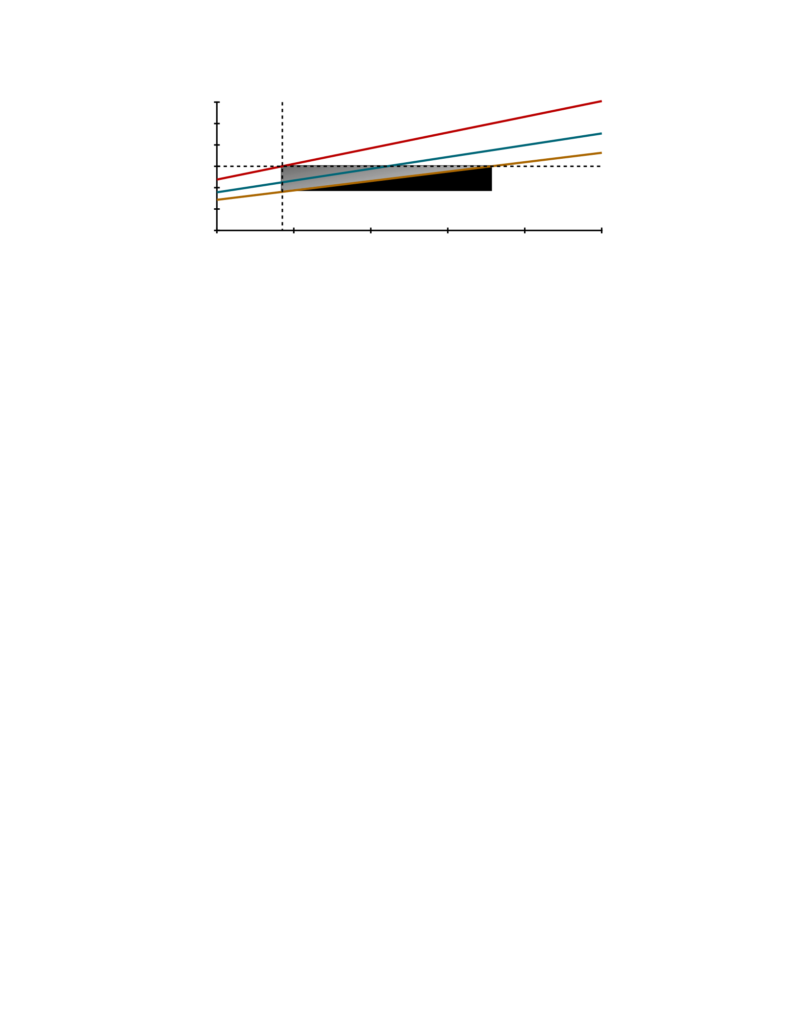
Physical constraints limit sensor data. Ground sample distance (GSD) is the geographic distance between
adjacent pixel-centers and a key figure of merit for visual data. Monolithic systems have GSDs
Pixel Sensor Side Length: 1.1 μm
CHAPTER 3. SATELLITE DATA QUALITY AND MACHINE LEARNING 16
Figure 3.1: Top: Image data quality is physically limited. Bottom: The OEC design space: volume, mass, power, and
cost of LEO 3U OEC devices. OEC is limited in volume and energy, but not mass or cost.
around 0.3 m/px [62], and cubesats have GSDs around 3.0 m/px [180]. Three parameters govern GSD: orbit
altitude, camera focal length, and pixel sensor size. GSD merit is proportional to focal length and inversely
proportional to altitude and sensor size. Orbit altitude depends on the mission. A cubesat typically orbits in LEO
between 325 km and 825 km. A higher altitude increases mission duration but degrades GSD. Below 400 km, a
cubesat reenters the atmosphere in weeks; one above 400 km can operate for years. Camera focal length is limited
by cubesat volume consumed by other systems, such as the attitude determination and control system (ADACS)
and batteries. Sensor technology is mature; this work assumes a COTS pixel sensor side length of 1.1 µm with at
least 4096 × 3072 pixels [178].
Figure 3.1, top, shows the OEC design space assuming a 3U volume (like commercial systems [61]), and
computes GSDs using a pinhole camera model [90]. Each curve is a different camera focal length. The data show
that a viable 2U camera system has a GSD of 2.26 m/px: 7.5× worse than monolithic satellite data, but comparable
to existing cubesat constellations.
System Architecture. This work proposes a simple, yet versatile OEC architecture. Based on volume and GSD
constraints, this work allocate 2U to camera equipment for a GSD ≤ 3.0 m/px. The remaining 1U contains the
ADACS, radio, and computing hardware. This work proposes using a fast commodity mobile GPU (e.g. GP10B Tegra
GPU) optimized for deep neural network (DNN) inference, a key OEC workload. A commodity X-Band radio and a
mobile GPU each consume over 7.5 W: slightly too high to run continuously and far too high to run simultaneously
with 7.1 W from a solar array. This work proposes a power system without a battery to avoid related volume, mass,
and management hardware and opts for small, dense supercapacitors. Supercapacitors buffer energy, permitting
high-power bursts of operation once charged. An OEC system computer sleeps while solar panels charge
supercapacitors, and it runs in bursts until energy is depleted. Charge time and burst time are dictated by panel
power and supercapacitor size, similar to intermittent computing [46].
GSD (m/px)
0.0
1.0
2.0
3.0
4.0
5.0
6.0
Orbit Altitude (km)
325 425 525 625 725 825
High Temporal Resolution
Camera System Design Space Commercial Systems
Contemporary

CHAPTER 3. SATELLITE DATA QUALITY AND MACHINE LEARNING 17
3.1.2 Downlinking Does Not Scale
Downlinks limit OEC constellation sensor datarate. Each cubesat must store data until near a ground station.
Existing systems downlink all images, incurring a 5.5 h delay before data reach customers [61]. Large constellations
amplify scalability challenges [138] because devices share a link and downlinking all data is infeasible as
constellations grow. Earth-observing satellites use polar orbits to maximize geographic coverage and sun-
synchronous orbits for constant pass times [28]. A satellite at 410 km maximizes spatial resolution with a GSD
under 3.0 m/px, has a temporal recurrence cycle of 2 d, and has an orbit period of 92.9 min. Fixed ground stations
have downlink windows of 10 min per device [61]. Existing systems downlink at 200 Mbit/s, receiving up to 15 GB
of data per pass. A ground station optimally positioned to observe every pass (e.g. a polar station for a polar orbit)
supports up to 9 satellites per revolution. Similarly supporting a 1000-satellite constellation requires 112 ground
stations. Provisioning many ground stations is wasteful if downlinked data are unused.
OEC reduces ground station count by computing on orbit and discarding uninteresting data early. If early
discard reduces 15 GB of raw data to 0.75 GB of useful data, all data downlink in 30 s at 200 Mbit/s. Each station
services 185 satellites per 92.9 min revolution. Equipped to compute, a constellation of 1000 OEC satellites is
adequately supported by 6 ground stations — increasing downlink capacity by 20×.
3.2 Optimizing Orbital Edge Computing
This work develops support for processing high-rate data in OEC constellations. Tiled image processing can be
tuned empirically to maximize accuracy. Intelligent early discard avoids processing uninteresting sensor data. OEC
pipelining parallelizes work across a constellation, mitigating latency.
Figure 3.2: The ground track frame rate, tiling, and cubesat pipelining.
3.2.1 Geographic Tiling to Maximize Accuracy
OEC systems split camera frames into tiles of fixed geographic area and scale each tile to the input size of an
inference kernel, like terrestrial satellite image processing [246]. Tile size determines feature (e.g. building) size
after scaling; smaller tiles have more pixels per feature after resizing, and larger tiles have fewer. Tile size
determines tile count per frame, which varies latency. Section 3.3 shows that tiling dictates accuracy and latency,
and some cases have an empirically optimal tile size.

CHAPTER 3. SATELLITE DATA QUALITY AND MACHINE LEARNING 18
3.2.2 Intelligent Early Discard
An OEC system avoids redundant tiles by capturing images at no greater rate than the ground track frame rate
(GTFR). The GTFR is the rate at which entirely new geographic scenes appear in the camera view, and the ground
track frame period (GTFP) is its inverse. Figure 3.2 illustrates tiling and the GTFR.
An OEC system processes images to filter uninteresting data, akin to recent drone-based systems [24, 255]. Earth
observation missions may have very specific targets (e.g. building footprint detection [246]) or broad goals (e.g.
Doves imaging Earth’s landmass daily [138]). In most cases, some images are not useful. For example, Doves avoid
imaging large water bodies based on location. However, Doves downlink images above land regardless of content.
Processing data before downlink as in OEC allows contentbased filtering. With OEC, images obscured by clouds can
be discarded as in [252]. An OEC disaster relief mission can find and downlink building coordinates instead of raw
images (Section 3.3.3 evaluates this
goal).
3.2.3 Computational Nanosatellite Pipelines
An OEC system can leverage ample existing work on reliable formation flying [15, 151] to keep nanosatellites in a
line and parallelize image processing across a constellation. Parallelism reduces effective frame latency. Each
satellite captures an identical frame at the GTFR, processing a subset of frame tiles statically determined by satellite
position in the linear formation. A frame’s tiles should be distributed across nanosatellites in proportion to their
computing capability; identical satellites process equal tile shares. A key advantage of OEC pipelining is that
satellite GPS location determines when to capture a frame and static pipeline position determines the tile subset,
requiring no satellite-to-satellite cross-linking to process data in parallel. Subframe latency, the latency for one
satellite to process its assigned tiles, is given by single tile processing latency, times the number of tiles per frame,
divided by pipeline depth. The pipeline completely processes an image before the next frame when subframe
latency is less than the GTFP. An OEC pipeline should have enough satellites to meet this requirement. Figure 3.2
shows an OEC pipeline in which each device processes only a subset of the frame tiles.
A computational nanosatellite pipeline requires propulsion and positioning. Recent surveys of deployed and
proposed nanosatellite propulsion systems make formation flying feasible [239, 15]. Contemporary, low-power
COTS navigation constellation receivers provide positioning for image capture triggers once unlocked for high
velocity, high altitude use [265].
CHAPTER 3. SATELLITE DATA QUALITY AND MACHINE LEARNING 19
3.3 Evaluation
This work evaluates an OEC system designed for image classification [229], object detection [232], and pixel
segmentation [141], running on the Jetson TX2 mobile GPU module, which prior work shows is robust to space
radiation [253]. It uses satellite data from SpaceNet [246] to train the networks. This work uses SpaceNet
evaluation metrics and ground truth for evaluation on separate SpaceNet test data.
Classification
100000
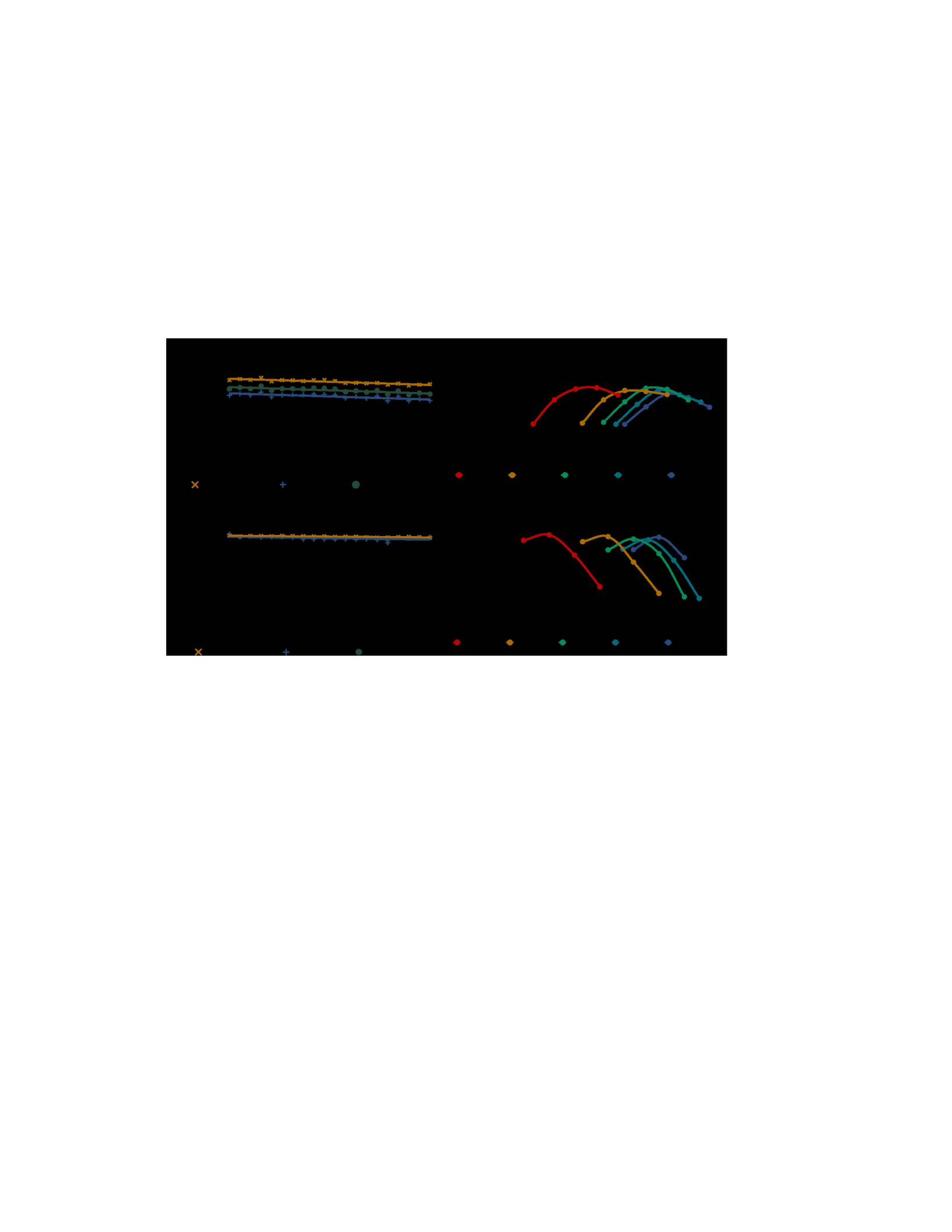
Figure 3.3: Left: Accuracy is stable as GSD degrades. Right: Tile area dictates tile count, determining latency.
3.3.1 OEC Maintains Accuracy
Despite physical limitations on achievable nanosatellite GSD, inference accuracy remains comparable to that on
higher quality monolithic satellite data. Figure 3.3, left, shows inference precision, recall, and F1 score [120] as GSD
varies. In each case, F1 score remains steady as GSD degrades from 0.3 m/px to 6.0 m/px, with only a slight
downward trend. Any modest decrease in F1 score due to lower GSD is likely acceptable given the 10,000×
decrease in OEC device cost and higher temporal resolution compared to monolithic systems.
Figure 3.3, right, shows how to optimize an OEC system tiling scheme for F1 score and latency. Tile size
determines latency. Across GSD values, there is a “goldilocks” optimal tile size maximizing F1 score for detection
and segmentation workloads. Smaller tiles increase latency without increasing F1 score, and larger tiles decrease
latency at the expense of F1 score. Given computing performance parameters, orbit parameters, and
representative data, a mission engineer can optimize tile size empirically before launch.
CHAPTER 3. SATELLITE DATA QUALITY AND MACHINE LEARNING 20
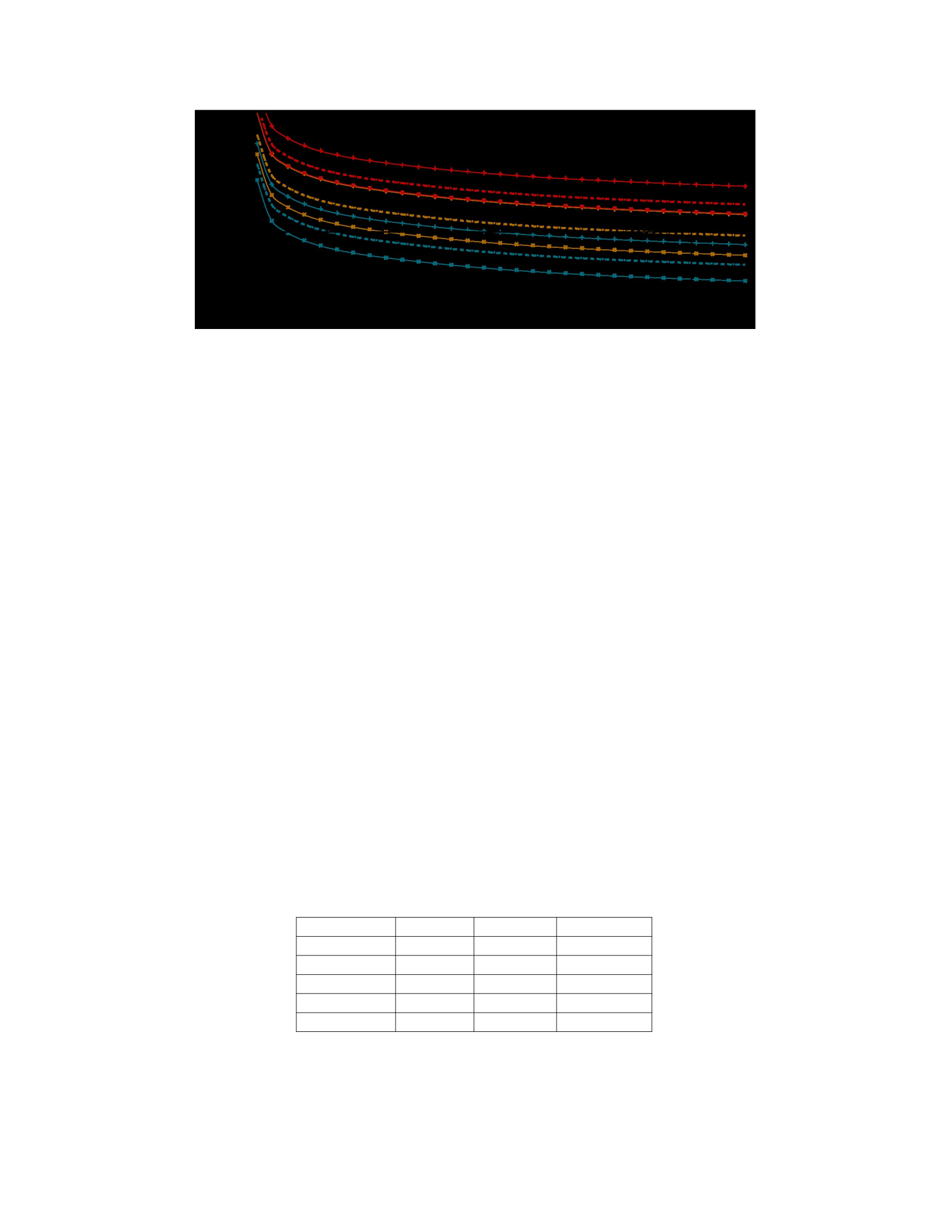
Figure 3.4: Top: Pipeline depth determines frame processing latency. For each workload (segmentation, detection,
classification), the number of Jetsons (1J/3J), input power (1P/3P), and energy storage capacity (5F/15F) vary.
Configuration 1P corresponds to 7.1 W, and configuration 3P corresponds to 21.3 W. Energy storage capacities are
in farads. Bottom: The amount of data transmitted depends on the filtering technique. Different filtering
techniques lead to different energy tradeoffs.
3.3.2 OEC Pipelines Mitigate Latency
OEC pipelines parallelize processing and effectively amortize frame latency. Figure 3.4, top, plots frame processing
latency versus pipeline depth. This work evaluates a pipeline in a 400 km altitude polar orbit with a 7.23 km/s
ground track velocity [28], a GTFP of 1.70 s, and a GTFR of 0.59 fps. It models full system behavior, including a
supercapacitor-based power system (using capacitor charging equations), and requires compute components to
sleep until capacitors charge. This work uses directly measured Jetson module power values to study systems with
one or three Jetsons (1J/3J), 7.1 W or 21.3 W solar arrays (1P/3P), and 5 Farad or 15 Farad energy storage
capacitors (5F/15F).
The data show that building detection is feasible at the GTFR, but that segmentation latency is infeasible at the
GTFR without increasing pipeline depth beyond existing systems. With a single GPU, low energy storage, and a
single solar panel, continuous object detection at the GTFR is feasible with a 245 satellite pipeline. With low energy
storage and a single panel, the workload consumes energy quickly, requiring more sleep periods to recharge and
increasing frame latency. With larger, folding, deployable Table 3.1: Accelerators enable shorter pipelines.
Accelerator Energy (mJ) Latency (ms) Pipeline Depth
Jetson TX2 [177] 643.3 42.89 78
ShiDianNao [65] 0.457 1.430 3
Origami [31] 0.722 1.415 3
EIE [87] 1.980 3.299 6
Eyeriss [36] 0.928 3.338 7
panels (3P), detection at the GTFR is feasible with 78 OEC devices — even allowing continuous operation while not
in eclipse. Classification is feasible at the GTFR in all configurations, with as few as 19 devices.

CHAPTER 3. SATELLITE DATA QUALITY AND MACHINE LEARNING 21
3.3.3 Performance Optimizations at the Orbital Edge
Intelligent early discard decreases network traffic and total energy. This work runs classification to find images with
buildings as a filter for building detection, and compares to sending all data, sending images with buildings, and
sending building coordinates only. Figure 3.4, bottom, plots the network traffic and total energy of an existing and
OEC system. With a varied fraction of interesting tiles (i.e. with buildings), sending coordinates only greatly reduces
network traffic. With classification, network traffic depends on the fraction of interesting tiles. Energy also depends
on the fraction of interesting tiles: below 30%, filtering avoids expensive detection. Above 30%, classification
filtering increases total energy cost when detection is also performed.
Architectural accelerators promise to optimize inference computations. Table 3.1 collects energy and latency
data from prior work to estimate the performance impact of acceleration in an OEC system.
Acceleration greatly decreases energy cost, avoiding sleep states and decreasing pipeline depth.
3.3.4 Hardware and Software Design Factors
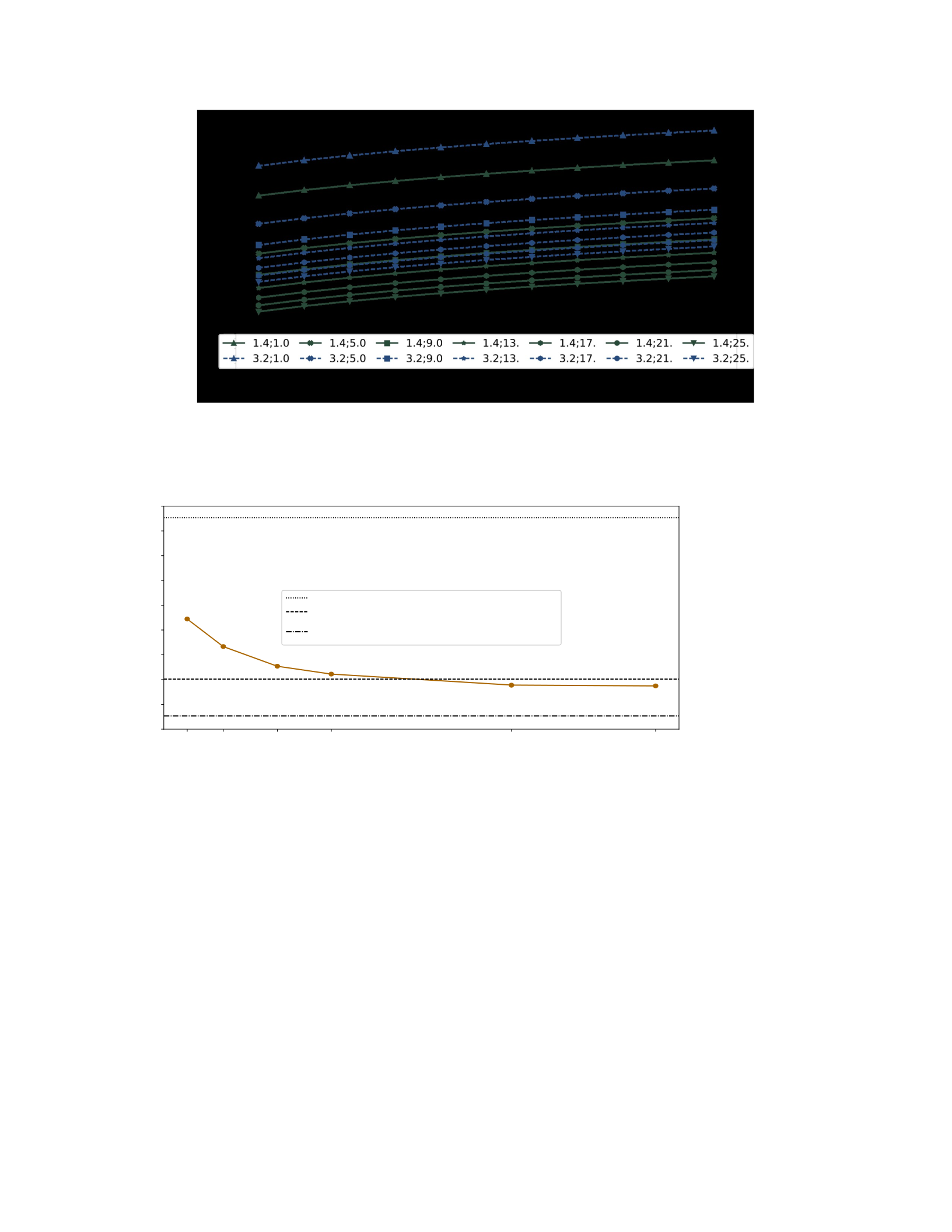
Camera system design space: Figure 3.5 illustrates a camera system design space. Pixel sensor size, camera focal
length, and orbit altitude impact data quality (GSD). Smaller sensor size improves GSD, but physics bounds
minimum pixel sensor size, and signal-to-noise ratio (SNR) worsens with smaller pixel size. Longer focal length
improves GSD, but SWaP-C limit maximum focal length; Section 3.3.4 shows that computational factors also affect
focal length choice. Lower orbit altitude improves GSD but shortens mission duration because more air resistance
hastens satellite reentry.
Computer system design space: Nanosatellites often harvest energy slower than an embedded computer
consumes energy, requiring a duty cycle. For a camera with a 20 cm focal length and a 4096 × 3072 px array,
changing pixel sensor size from 1.4 µm to 3.2 µm and changing orbit altitude from 343 km to 600 km worsens GSD
from 2.4 m/px to 9.6 m/px. The ground track frame period (time between en-
CHAPTER 3. SATELLITE DATA QUALITY AND MACHINE LEARNING 22
Figure 3.5: Satellite image quality ranges from 1.68 m/px to 256 m/px by adjusting physical system properties.
Computer System Design
Space; Ops/Exec: 0.2e14
Operations per Second; Power Draw (W); Duty Cycle (Uptime Fraction)
Figure 3.6: Lack of power reduces performance. Accounting for feature size changes deadlines by 10× or more.
tirely new geographic areas entering the camera view) eases from about 1.0 s to about 4.3 s. However, as Section
3.3.5 shows, processing frames naively gives significantly different system performance (e.g., in accuracy). Keeping
accuracy largely constant by duplicating pixels in the worse image to match feature sizes in the better image, the
deadline per tile becomes about 0.27 s — unachievable for all computer systems in Figure 3.6.
0.2e14
10
0.45
0.4e14
15
0.30
0.7e14
20
0.23
1.0e14
25
0.18
2.0e14
40
0.11
2.8e14
55
0.08
0.0
0.5
1.0
1.5
2.0
2.5
3.0
3.5
4.0
4.5
Execution Time with Duty Cycle (s)
Naive deadline (one tile per 9.6 m/px frame)
Naive deadline (one tile per 2.4 m/px frame)
Per-tile deadline (9.6 m/px) after scaling to
match feature sizes in 2.4 m/px frame
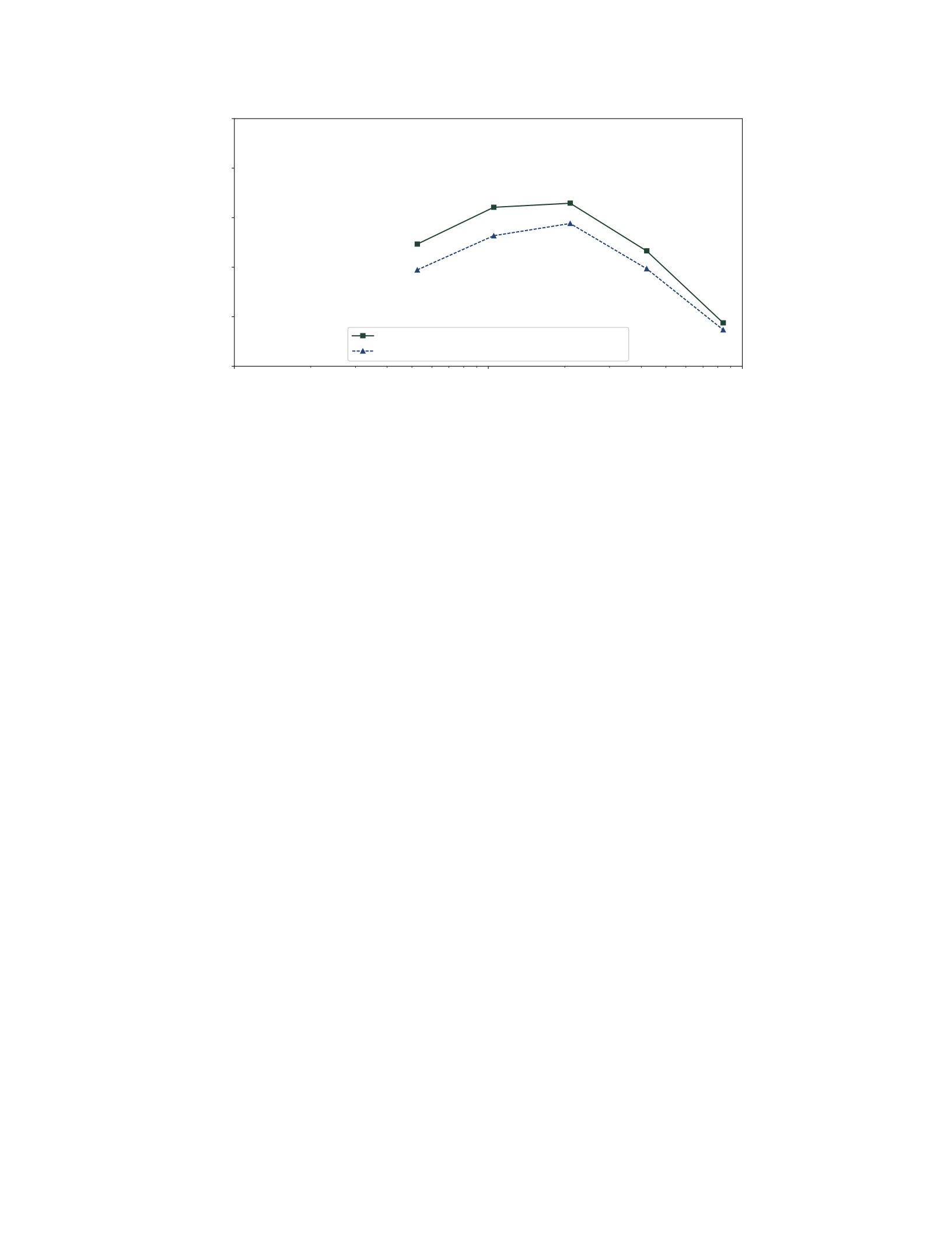
CHAPTER 3. SATELLITE DATA QUALITY AND MACHINE LEARNING 23
System
Performance: Object Detection, 192 px NN Input Size
Figure 3.7: Feature size (pixel count) impacts accuracy more significantly than feature resolution (visible details).
3.3.5 System Performance
A 4× worse GSD system scales image width and height by 4× (e.g., pixel duplication) to avoid smaller feature sizes
(at the cost of more “blurry” features); see Figure 2.1. This system has either (i) different accuracy due to different
target feature size (pixel count), or (ii) different execution time due to different total frame pixel count after scaling
to compensate for feature size; see Figure 3.7. Prior work [51] benefits from this ML accuracy/execution time
tradeoff. Feature size (distinct from feature resolution) is an active area of CV research [33].
This tradeoff space is largely unique to satellites. Images and videos from social networks and media sites
naturally contain features with pixel counts that are neither too small nor too large. Video surveillance [35, 4, 256]
and drone video [255, 79] may encounter feature size and image quality challenges. However, video surveillance
could address these challenges with longer camera focal lengths, and drone video could address these challenges
by flying closer to targets.
3.4 Summary
This work develops orbital edge computing. The low cost of nanosatellites compared to monolithic satellites makes
large constellations feasible for the first time. Applications of this emerging technology are impeded by traditional,
centralized architectures. Orbital edge computing provides responsiveness, reliability, and scalability benefits.
Future work should study energy collection and storage for orbital edge computing and radiation hardened
machine learning accelerators. Cubesat pipelining may motivate fur-
10 010 110 2
Average Target Feature Size (px)
0.0
0.2
0.4
0.6
0.8
1.0
F1 Score (IoU Metric)
3.0 m/px GSD (Compare to Camera A Frame )
6.0 m/px GSD (Compare tp Camera B Tile 10)

CHAPTER 3. SATELLITE DATA QUALITY AND MACHINE LEARNING 26
ther research in nanosatellite control and orbital cross link communication.

Chapter 4
Machine Inference in Space
The proliferation of commercial space launch services [78] and nanosatellites [167, 186] over the past two decades
makes low-Earth orbit (LEO) accessible to deployments of state-of-the-art, sensor-equipped computer systems
inside satellites. These satellites enable new and valuable geospatial sensing and computing applications, including
disaster relief [86], agriculture [248], and infrastructure monitoring. The Earthobservation market remains
dominated by large-scale, monolithic satellites costing hundreds of millions of US dollars each. However, the
ascendance of inexpensive nanosatellites has led to large, commercial constellations of nanosatellites in LEO [29,
138]. Lower device cost and higher launch cadence decreases risk and enables new satellite applications [148].
Communication and computation ability constrain satellite utility. Today, most satellites operate as “bent pipes”
[136] and are tasked manually to collect and downlink raw sensor data. These satellites face a downlink bottleneck
stemming from a lack of communication opportunities. Recent work on “orbital edge computing” (OEC) processes
data on satellites before downlinking [52, 53]. OEC mitigates the downlink bottleneck by identifying signals of
interest and downlinking those signals only. While OEC addresses the downlink bottleneck, edge processing creates
a computational bottleneck limiting the value of each satellite.
Processing satellite sensor data at the edge is challenging. Satellite sensor samples (e.g., images) are large and
arrive at a high rate compared to the rate at which embedded satellite hardware can process them. Geospatial
image frames can contain hundreds of square kilometers and hundreds of millions of pixels. Depending on orbit
altitude and camera characteristics, a LEO, Earth-observation satellite observes an entirely new frame every 1 − 30
seconds (the “frame deadline”). Applications typically tile these large frames and process each tile on the ground
using, e.g., machine learning algorithms. However, not all samples are equally valuable; some observations are of
high-value to an application and others are of low-value. A system faced with a saturated link should prioritize
transmission of high-value data,
27
but today’s bent pipes send data indiscriminately. Processing samples at the space edge distinguishes these
categories. The computational bottleneck stems from an inability to process all tiles within the frame deadline.
Prior OEC work manages the computational bottleneck by statically distributing tile processing across a
constellation, using satellite-parallelism to meet the frame deadline [53]. Such a scheme distributes work across

CHAPTER 4. MACHINE INFERENCE IN SPACE 26
hundreds of satellites while addressing the computational bottleneck for just a single application — a relatively
high-cost solution resulting in a vertically-integrated constellation aimed at a particular purpose.
Kodan is an orbital edge computing system that maximizes data value from satellites limited by communication
and computation. Under a saturated satellite downlink, Kodan mitigates the computational bottleneck without the
high cost of hundreds of satellite-parallel processors. Kodan uses a combination of techniques that modify
applications based on unique, orbital data characteristics by trading between geospatial analysis precision and
processing speed. After deployment to a satellite, the Kodan runtime system dynamically selects appropriate
optimizations for each observation. Kodan decides how to process a sample based on its geospatial context. A
geospatial context is a property of a data sample indicating its likelihood to contain certain features, e.g., the
presence of ocean, forest, tundra, clouds, or high-value data. High-precision value labels are computationally easier
in some contexts and harder in others.
Kodan balances precision and execution time to maximize data value density. Software running on each satellite
prioritizes decreased compute time when computationally bottlenecked and prioritizes precision otherwise. When
computationally limited, Kodan uses tile context to select an action: the satellite downlinks data in high-value
contexts, discards data in low-value ones, and executes an application to more thoroughly filter the rest. Whether
or not computationally limited, Kodan uses context-specific models to increase precision and downlinked data
value density, i.e., the fraction of a saturated downlink composed of high-value bits. Kodan recognizes that not all
sensor data need equal care in processing. To trade precision for execution time, Kodan adjusts frame tile count to
reduce data quantity at a cost in quality.
Kodan increases downlinked data value density by mitigating the computational bottleneck. To show the value of
Kodan, this work implements seven end-to-end, deployment-ready, pixel-segmentation applications trained to
filter low-value clouds using publicly-available, geospatial datasets. This work quantifies the improvement in
valuable data downlinked with on-orbit computing using context-specialization to identify high-value observations;
Kodan improves the data value density of the saturated downlink between 89 and 97 percent compared to the
bent pipe.
To summarize, the primary contributions of this chapter are: (i) a characterization of the impact of

CHAPTER 4. MACHINE INFERENCE IN SPACE 27
Figure 4.1: A satellite periodically captures image frames, and the time between frame captures is the frame
deadline. Before processing an image, geospatial analysis software splits a frame into tiles. Details visible in the
images depend on the ground sample distance, or the geographic area per pixel.
orbital edge computing on both the downlink bottleneck and the computational bottleneck; (ii) Kodan, an OEC
system that addresses the computational bottleneck using hardware-aware modifications of satellite applications;
(iii) a characterization and evaluation of context-specific models, frame tiling, and contextbased elision to maximize
data value density within the constraints of the computational bottleneck; and (iv) a comprehensive evaluation of
Kodan across satellite data processing applications and hardware targets, resulting in improvements to the data
value density of the saturated downlink between 89 and 97 percent.
4.1 Background and Motivation
This section provides context for Kodan and characterizes challenges for Earth-observation satellites.
Earth-observation satellites: LEO, Earth-observation satellites collect sensor data — e.g., multispectral images —
for geospatial analytics. These satellites often deploy to polar orbits (i.e., orbits crossing near the poles of Earth). As
the satellite travels through its orbit, it accesses nearly all latitudes; as the planet rotates, the satellite accesses all
longitudes. LEO altitudes are hundreds of kilometers, and LEO periods are about 90 min.
Historically, Earth-observation satellites are large and monolithic. Recently, inexpensive nanosatellites have
proliferated. The monolithic Worldview [74], Earth-Observing 1 (EO-1) [168], and Landsat [144] satellites cost
hundreds of millions of US dollars each (e.g., $855,000,000 [91]). Now, many missions use
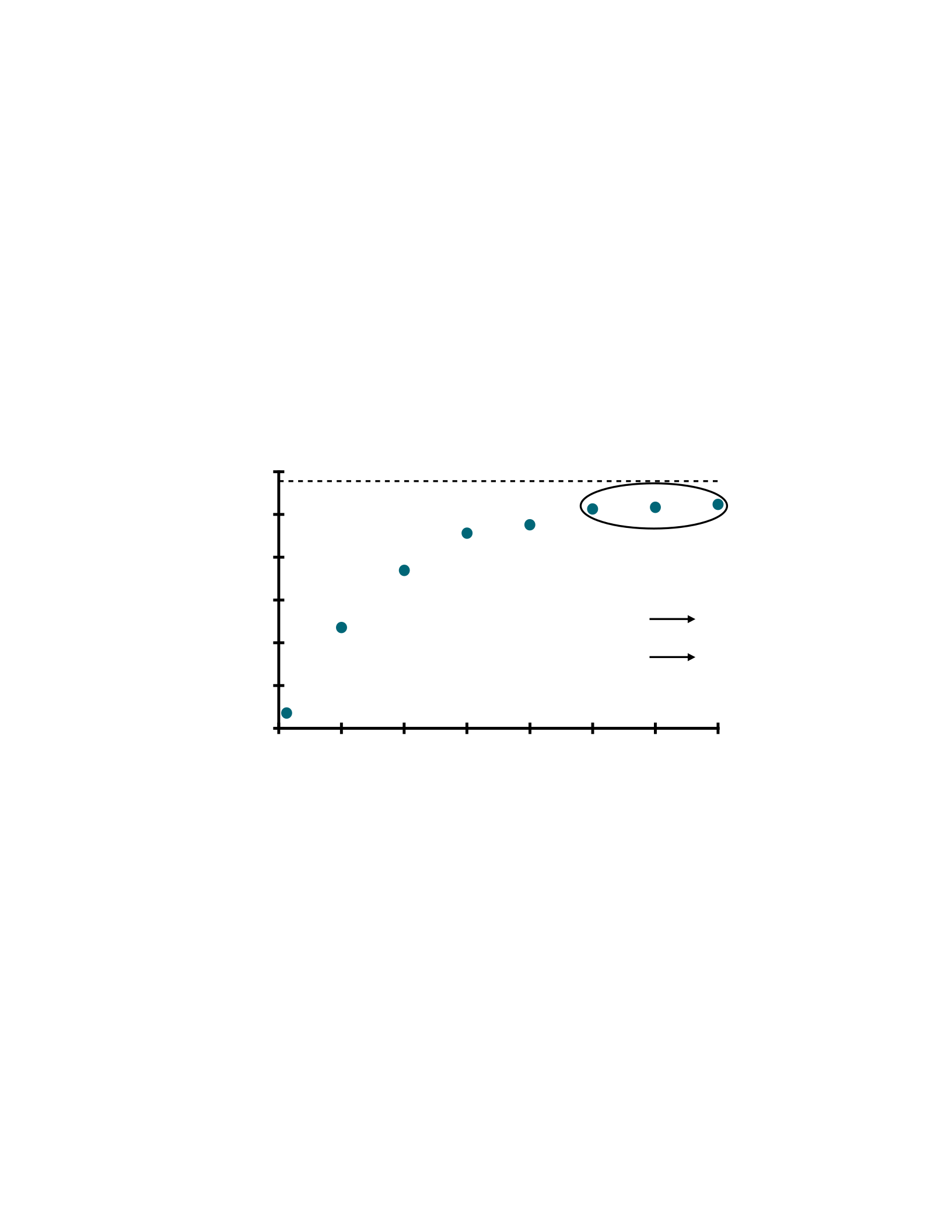
Global Frames per Orbit Period
Satellite Count
Figure 4.2: A single satellite observes more frames per revolution than it downlinks. As satellite count increases,
contention and eventually ground segment saturation widens this gap. Note the y-axis log scale.
cubesats [167], chipsats [267], and pocketqubes [186, 57] to increase hardware refresh cadence and avoid the high
costs of monolithic satellites. Lower costs enable Earth-observing constellations consisting of hundreds of devices
[29, 138].
Orbital mechanics determine both access to and the quality of satellite sensor data. For images, a satellite
captures a frame along its ground track. A frame is a large geographic region; geospatial applications often split
frames into many smaller tiles for analysis. Satellite image quality is characterized by ground sample distance (GSD)

CHAPTER 4. MACHINE INFERENCE IN SPACE 28
— geographic distance between adjacent pixels — which may range from km/px to cm/px [144, 74] and is
determined by altitude and camera characteristics. Figure 4.1 illustrates these concepts.
The bent pipe: Today, most Earth-observation satellite operators manually task their devices to sense and downlink
raw observations to a datacenter for processing, i.e., a bent pipe [136, 61]. Communication opportunities for high-
velocity, LEO satellites last only for a few minutes while the device is near a ground station and may occur
infrequently depending on the orbit. State-of-the-art communication systems downlink a total data quantity of
MBs or GBs per pass. This downlink bottleneck constrains observation rate because not all data can be sent (Section
4.1.1 quantifies this bottleneck).
Orbital edge computing: Recent work proposes orbital edge computing (OEC) [52, 53], in which satellites process
data at the space edge. OEC distributes computation across a constellation where each satellite contains highly-
capable, commercial, off-the-shelf (COTS) compute hardware rather than lowperformance, radiation-hardened,
space CPUs. An OEC satellite tiles each image frame and processes tiles to identify interesting data to transmit.
Especially when interesting features are rare, OEC addresses the downlink bottleneck with edge computing by
triaging sensor data before transmission. However, OEC must process all frame tiles before a new frame enters the
sensor view, creating a frame processing deadline usually between 1 − 30 s. Failing to meet the deadline is a
computational bottleneck.
4.1.1 Challenges at the Orbital Edge
This section highlights two orbital edge challenges: a downlink bottleneck prevents sending all raw data, and a
computational bottleneck prevents processing all data on orbit. These bottlenecks are quantified using the cote
[53] simulator to model existing satellites, including orbital dynamics, sensing, communication, and the ground
segment. This work validates the analysis with publicly-available satellite and ground segment performance metrics
[144]. This section addresses three key questions:
1. What limitations arise from today’s downlink bottleneck, and what will its impact be in the future (Section
4.1.1)?
2. To what extent could edge computing address the downlink bottleneck (Section 4.1.1)?
3. How much of this potential improvement can be realized by directly deploying data processing applications to
the space edge, and to what extent does the computational bottleneck limit these improvements (Section
4.1.1)?
CHAPTER 4. MACHINE INFERENCE IN SPACE 29
The Downlink Bottleneck
Downlink capacity cannot support existing satellite sensor datarates, and the gap grows with sensor fidelity and
constellation population. Figure 4.2 quantifies this gap for Landsat 8. Over one orbit revolution, the ground
segment supports reception of just 2% of the available observations of hyperspectral, 10K image frames. When
satellite count in the same orbit plane increases from one to 16, downlinked data increases from 5 frames during
one period to 60 frames during the same period; this improvement stems from claiming previously idle ground
station time. When the Landsat ground segment serves one satellite, stations sit idle while the satellite is out of
range (i.e., most of the time). Additional satellites, when not contending with each other, claim idle time and
increase total downlinked data. However, as constellation population increases, the space segment eventually
saturates the downlink. Adding satellites beyond this
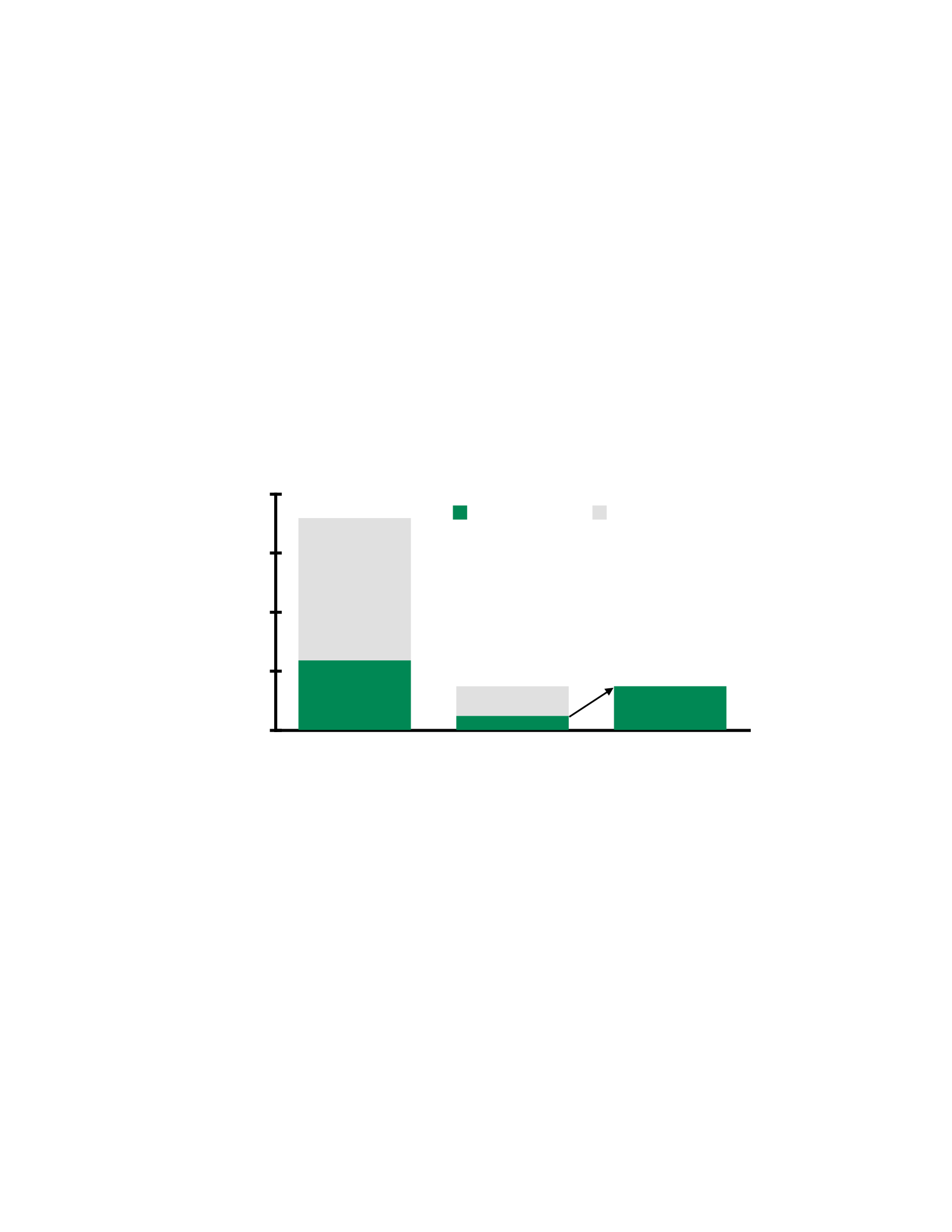
Global Unique Frames Observed per Day
Satellite Count
Figure 4.3: For the first time, constellations exist with enough satellites to achieve daily global coverage. Saturated
downlinks lock these daily global observations at the orbital edge.
population count increases the ability to observe but not downlink additional data, widening the downlink gap.
Why are large constellations desirable? Larger constellations increase sensor coverage of Earth. Figure 4.3 shows
the satellite count required for daily global coverage, i.e. the opportunity to observe all Landsat frames each day
(see Section 4.1.1 for discussion on whether such observations could be downlinked). This work adds support to
cote for the Landsat Path/Row World Reference System (WRS) [223] and imports the WRS-2 scene boundary
shapefiles to produce this plot. Reaching global daily coverage requires a constellation population of at least 40.
Frame Count
0
10000
20000
30000
40000
50000
60000
0 8 16 24 32 40 48 56
Total Unique Global Frames
Daily Global Coverage
Spire “Lemur” Constellation (~120)
Planet “Dove” Constellation (~200)
CHAPTER 4. MACHINE INFERENCE IN SPACE 30
Constellations in different orbits or with different sensors, like the Spire “Lemur” or Planet “Dove” satellites, deploy
even greater numbers of devices.
Addressing the Saturated Downlink
Bent-pipe satellites waste limited downlink capacity by indiscriminately sending observations containing both high-
value and low-value data. To demonstrate this fact, this work examines a cloud-filtering application. On average,
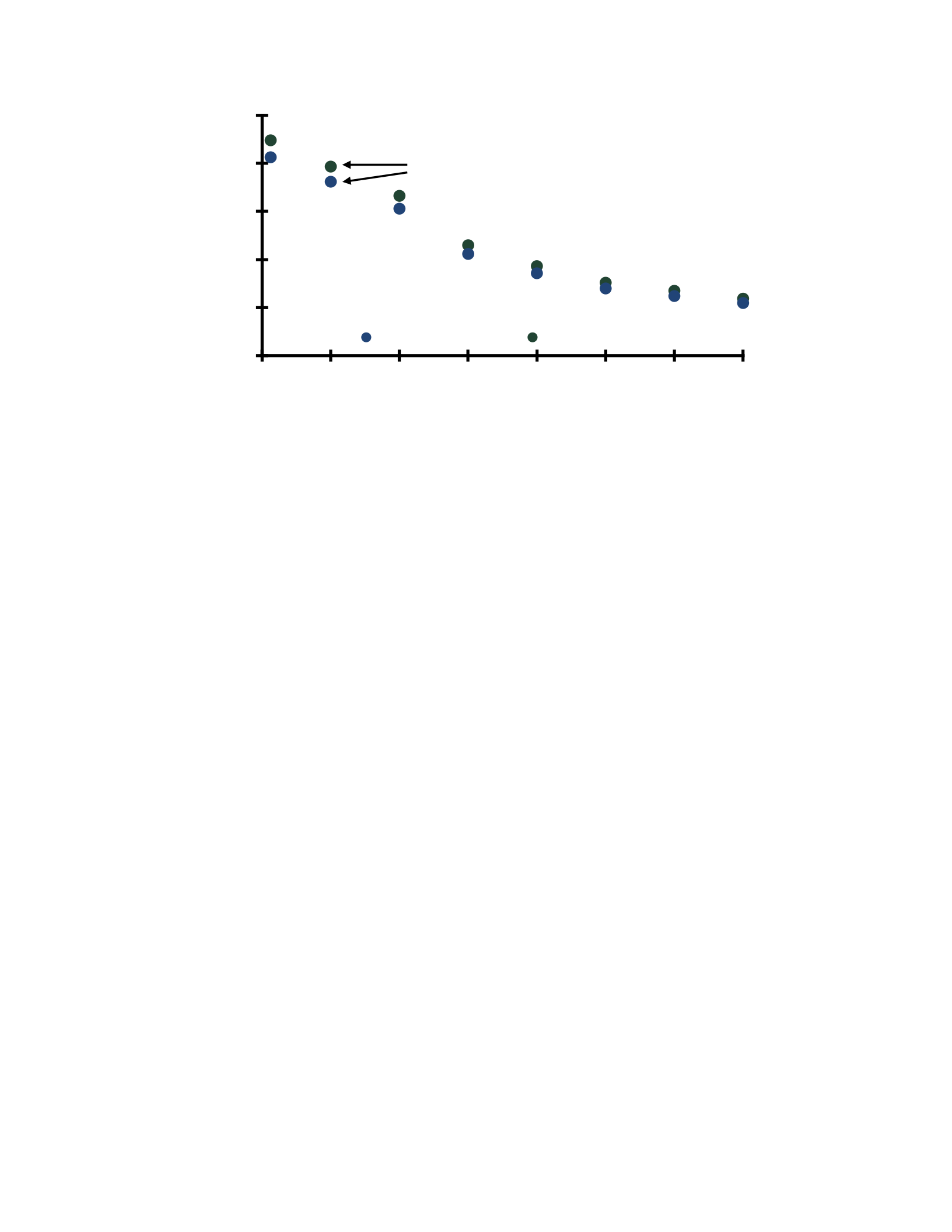
67% of satellite images are obscured by clouds [127] and are low-value to most customers. For Landsat 8, Figure
4.4 (left column) shows that, during one day, just 1/3 of the data from nearly 3600 observable frames is high-value
(i.e., not cloudy). Accounting for the downlink bottleneck (middle), less than 21% of observable high-value data is
downlinked with a bent-pipe. Ideal edge filtering (100% accuracy and zero execution time) delivers over 3× more
high-value data — 63% of the total,
Frames per Satellite per Day
Observed on Orbit Downlinked, Bent Pipe Downlinked, Ideal OEC
Figure 4.4: A single satellite observes more frames per day than can be downlinked per day. Many of these frames
contain low-value data. Without OEC, a relatively small amount of downlinked data is high-value (21%). Identifying
high-value data on orbit can improve the data value density by 3×.
Observed High-Value Data Downlinked
Frame Count
0
1000
2000
3000
4000
High-Value Data Low-Value Data
Edge filtering
provides up to
3x improvement
3x
CHAPTER 4. MACHINE INFERENCE IN SPACE 31
Figure 4.5: Directly deploying existing geospatial analysis applications to the inelastic orbital edge provides limited
improvement in saturated downlink utilization. These applications are designed for elastic datacenters and cannot
process data at the rate of new satellite observations.
observable high-value data, and the maximum possible under the downlink bottleneck (right column). Increasing
the ratio of high-value to low-value data increases the data value density of the saturated downlink: the fraction of
downlinked data composed of high-value bits.
The Computational Bottleneck
While ideal cloud filtering offers a potential 3× improvement in valuable data downlinked, the space edge must
contend with the inelastic and limited computational resources on satellites. Volume, mass, energy, and cost
constraints at the space edge prevent deployment of unlimited computational resources inside a satellite [53].
Unless a filtering application completes within the frame deadline, a satellite cannot process all frames, creating a
computational bottleneck that limits the ability of OEC to address the downlink bottleneck. This work quantifies
this effect for a real cloud filter application [164]. Figure 4.5 shows the fraction of high-value data downlinked with
and without edge filtering for a range of constellation sizes. Direct-deployment of cloud filtering improves high-
value data downlinked by just 9%, far short of the potential 3×. The shortfall stems from the 98 s frame processing
time, which exceeds the 22 s frame deadline; only a fraction of captured frames can be filtered. Therefore, while
OEC has potential to mitigate the downlink bottleneck, the computational bottleneck limits its benefit.
Limitations of parallel, distributed computation: Prior OEC work addresses computational needs by distributing
work across a pipeline of satellites. While effective at reducing per-satellite compute time to meet full ground track
coverage, pipeline populations must be very large (e.g., > 100 devices per application). This approach is costly and
designed for vertically-integrated constellations deployed for a single purpose. The future might see the emergence
Percent
0
5
10
15
20
25
Satellite Count
0 8 16 24 32 40 48 56
Bent Pipe Direct Deploy
Filter execution time: m 38s1 per frame
Result: %9 improvement
instead of x3 improvement
New frame observed every s22

CHAPTER 4. MACHINE INFERENCE IN SPACE 32
of constellations acting as a platform for customer applications, i.e., a constellation-as-a-service. As a result, the
naturally inelastic space edge has pressure to operate at its computational limit in order to maximize platform
value. Prior OEC work provides no technique to reduce per-satellite computational load without increasing
constellation population; this shortcoming is a key motivation for Kodan.
4.2 Kodan System Design
Kodan is an OEC system maximizing the data value density of a saturated satellite downlink by adjusting geospatial
analysis software to adapt to target satellite computing hardware in space. As constellation population increases to
eliminate idle ground station time, the ground segment becomes saturated, and additional satellites increase
observation opportunity but not downlinked data quantity. To increase the utility of this saturated downlink, the
fraction of downlinked data composed of high-value bits — the data value density — must increase. Distinguishing
between high-value and low-value sensor data on a satellite requires execution of geospatial analysis software at
the space edge. Unless a satellite processes each sensor sample before the next data capture, not all observations
are filtered: a computational bottleneck.
Satellites are edge devices in space; volume, mass, energy, and cost constraints prevent deployment of unlimited
computational resources [53]. Kodan reduces the computational requirements of geospatial analysis software
deployed to the space edge.
Kodan makes different adjustments to an application’s computational requirements for each hardware
deployment target. This approach is an alternative to simply increasing the computational capability of a satellite —
something that cannot be done for satellites already in space, and an option constrained by volume, mass, energy,
and cost limitations. This approach is also an alternative to simply increasing the number of satellites in a
constellation and distributing processing, which incurs high monetary cost and only addresses constellations
executing a single application.
To adjust the computational needs of a geospatial analysis application, Kodan leverages three techniques:
context-specific models, frame tiling, and context-based elision.
Context-based model specialization. This technique improves accuracy and precision of on-orbit inference by
training models specialized to contexts. A context is a subset of satellite images related by a high degree of
similarity in some semantically-meaningful way. For example, there is a high degree of similarity among images of
forested land and among images of the ocean, while there is relatively little similarity between an image of
forested land and an image of the ocean.

CHAPTER 4. MACHINE INFERENCE IN SPACE 33
Context-based model specialization provides accuracy and processing time benefits. A context-specialized model
yields higher accuracy on data from its context (see Section 4.4.3). Additionally, a specialized model may retain or
improve accuracy while being smaller and simpler, because the model is tailored to a smaller set of data. The ability
to use smaller models without degrading accuracy allows satellites to run complex legacy applications (e.g.,
applications designed for the datacenter cloud) with fast, simple models tailored to the inelastic space edge.
Frame tiling. This technique adjusts tile count per frame, which in turn affects the resolution of tiles input into
machine inference models. A satellite frame processing application divides the image into some number of tiles
and scales each tile to match the neural network input size. Prior work [52, 53] divides each frame into a tile count
maximizing inference accuracy. For each application, Kodan sweeps a range of tile counts and selects the count
maximizing downlinked data value density for the target hardware platform. When the application is not
computationally-constrained on the target hardware, data value density maximizes with the most precise tiling.
When the application is computationallyconstrained, data value density maximizes at a less-precise tiling with
lower total frame execution time (see Section 4.4.4).
For example, Figure 4.6 illustrates an application that processes a 10 000 px × 10 000 px Landsat image.
Figure 4.6: Tile count per frame determines frame processing time. A smaller tile count decreases frame processing
time, but each tile must undergo more decimation to match the neural network input size. A larger tile count
increases frame processing time, and each tile undergoes less decimation.
The figure illustrates either dividing the image into four tiles 5000 px × 5000 px in size or 16 tiles 2500 px
× 2500 px in size. After resizing each tile to the neural network input size, the processing time per tile is constant.
Thus, tile count determines frame processing time; a greater number of tiles per frame increases frame processing
time.
Tiling affects the quality of the sample input into a neural network. Fewer, larger tiles require more aggressive
decimation to match the input dimensions of the neural network. More numerous, smaller tiles support more
preservation of tile detail for neural network input.
Prior work [52] shows an empirically optimal tile count for accuracy, and that accuracy degrades as tile count
increases or decreases from this value. Section 4.4.4 shows that there also exists an empirically optimal tile count
for precision, and this tile count may differ from the empirically optimal tile count for accuracy. Further, empirically
optimal tile counts vary by model architecture.
Elision of processing based on sample context. This technique avoids execution of computationally-costly filtering
on data samples likely to be either mostly high-value or mostly low-value. Instead, Kodan discards images from
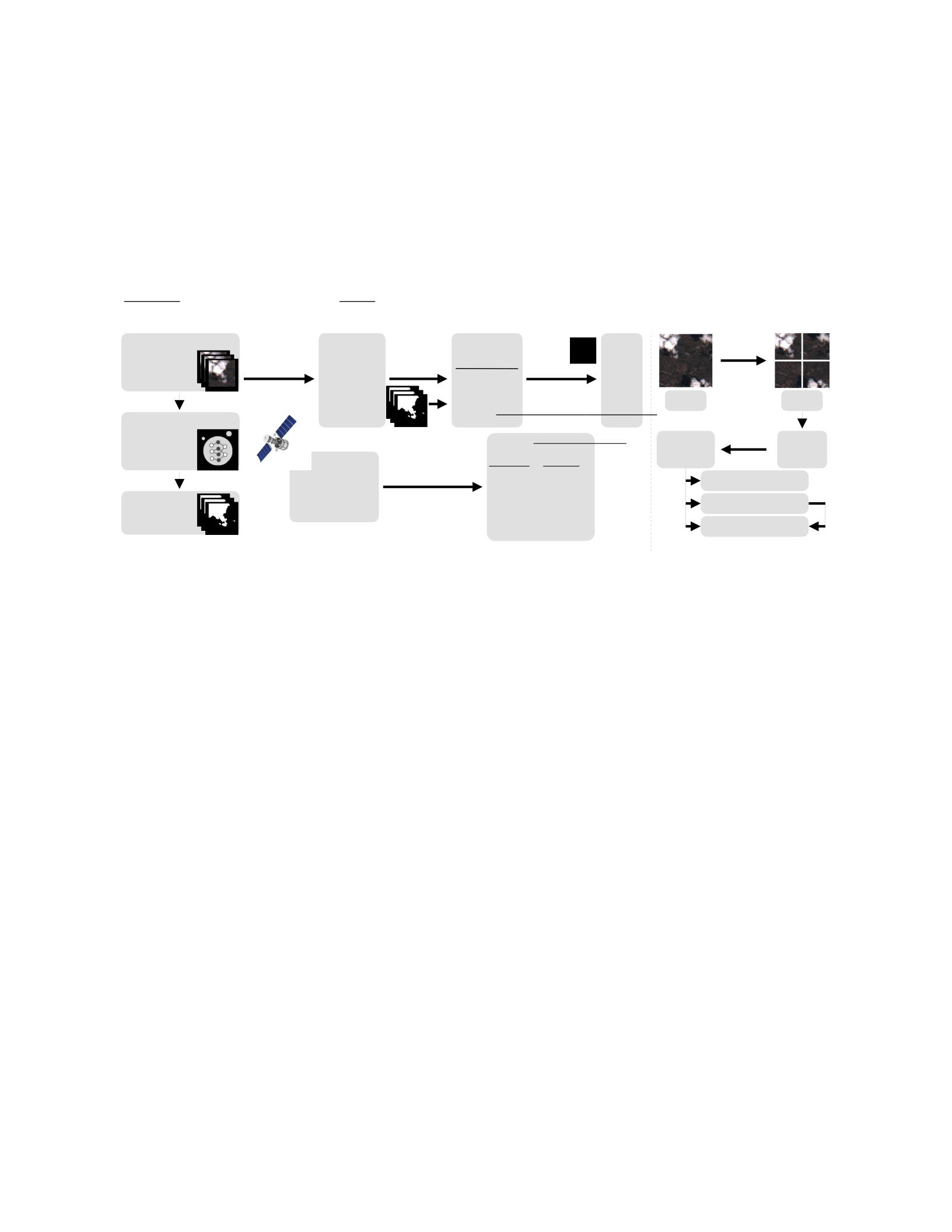
CHAPTER 4. MACHINE INFERENCE IN SPACE 34
contexts containing primarily low-value data and downlinks images from contexts containing primarily high-value
data. For example, an application searching for building footprints discards data from a context characterized by
heavy cloud cover and downlinks data from a context characterized by dense urban areas. Kodan leverages elision
by first identifying the tile context and then, if the tile belongs to a context with mostly high-value or low-value
data, elides execution of the filtering application.
Representative Clustering/ Geospatial Supervised Specialized Target Exec. Reference Unsupervised
Contexts Learning Models Prec. Satellite Times
Dataset Learning C1 (e.g. cloudy) M1 0.79 Hardware 178
C2 (e.g. water) M2 0.85 238
… … … … Frame Tiles
Geospatial Analysis Ci (e.g. land) Mj0.92 475
Reference Selection Logic Selection Context
Application Target Satellite Parameter Sweep• Frame Tile Count Frame Tile Count: N Logic Engine
System (HW, • Elision Choice Context Choice Discard
Orbit, Ground System Simulation C1 Discard
Truth Labels Segment) cote C…2 M…k Specialized Model
Goal: Max. DVD CiDownlink Downlink Queue
Before Deployment to Satellite After Deployment to Satellite
Figure 4.7: Left: Before deployment to a target satellite, Kodan performs a one-time transformation step.
This step clusters the representative dataset into contexts and generates a selection logic for maximizing DVD.
Right: After deployment to a target satellite, Kodan leverages the context engine and the selection logic to meet
the soft processing deadline.
Summary: Kodan leverages three techniques to maximize data value density by adjusting application precision and
execution time for each target hardware platform. Context-based model specialization improves data value density
via improved precision. When an application is not computationally-constrained, all data value density
improvements stem from improved precision. Sample-based processing elision skips lengthy filtering of samples
belonging to contexts characterized by large amounts of high-value or lowvalue data. When an application is
computationally-constrained, downlinking samples from a high-value context without filtering small quantities of
low-value data has the effect of slightly reducing precision while significantly reducing execution time and thereby
increasing data value density. Frame tiling also trades execution time and precision. When an application is not
computationally-constrained, Kodan increases data value density by selecting the empirically optimal tiling for
precision.

CHAPTER 4. MACHINE INFERENCE IN SPACE 35
4.2.1 Kodan System Architecture
Kodan improves the data value density of the saturated downlink within the computational constraints of a target
device by adjusting each geospatial analysis application as shown in Figure 4.7. A one-time application
transformation step occurs before deployment. During deployment, Kodan dynamically selects these application
adjustments for each sample.
Before deployment to a satellite: This one-time transformation step generates a “selection logic” that governs
how, when, and which techniques (specialized models, frame tile count, and context-based elision) to deploy on
orbit. Each geospatial analysis application is associated with a dataset representative of the distribution of input
samples. To transform the geospatial analysis application to maximize data value density when deployed to a target
satellite, Kodan (i) partitions the representative dataset into contexts; (ii) generates a context engine to classify
each tile into a context, and (iii) trains and validates context-specialized models. Then, given the characteristics of
the target satellite (computational capabilities, sensor and radio attributes, and orbit parameters) and its ground
segment, Kodan sweeps frame tile count and context-based elision options to identify the combination of
techniques maximizing data value density to produce the selection logic.
Section 4.2.2 details context generation and the context engine. To train and validate context-specialized models,
Kodan adheres to machine learning best practices as described in Section 4.3. Section 4.2.4 details the procedure for
generating the resulting selection logic.
After deployment to a satellite: During deployment, Kodan leverages the context engine and the selection logic to
dynamically select application adjustments for each data sample. Based on the selected tile count per frame,
Kodan splits each frame. The context engine classifies each tile into a context, which determines whether Kodan
executes a specialized model or elides further processing and either downlinks or discards the sample. The satellite
downlinks the application results during the next contacts with the ground segment.
4.2.2 Contexts and the Context Engine
Kodan must quickly and accurately classify each tile into a context for the selection logic to use when choosing
application adjustments to maximize data value density within the computational constraints of the target
hardware. This work presents two approaches for context generation and selection: expertgenerated contexts and
automatically-generated contexts.
Expert-generated contexts: In this approach, a subject-matter expert (SME) partitions the representative dataset
into human-recognizable contexts. This work observes that satellite images consist of a limited number of human-

CHAPTER 4. MACHINE INFERENCE IN SPACE 36
recognizable contexts that largely remain static over time. Course-grained examples include ocean views versus
land views; more fine-grained examples include mountains, deserts, and cities.
Using this approach, a sample context can be determined from satellite position and orientation, a geographic
map, and a projection of the expected satellite view onto this map. Thus, the context of each sample can be
determined at the orbital edge in real time with even modest computing hardware. Because satellite orbits are
highly predictable and can be modeled far in advance using tools like the cote simulator [53], the expert-selected
context of each sample could even be pre-computed. Expertselected contexts have the benefit of being human-
explainable and quickly determined for each data sample. However, there may exist applications in which expert-
selected contexts are not obvious or easy to generate.
Automatically-generated contexts: To support context generation and selection for general datasets without
dependence on human experts, Kodan automatically partitions datasets into contexts. In Section 4.4, Kodan uses
label vectors indicating the geographic and weather features present in each sample to cluster the representative
dataset by similarity. Kodan creates a set of contexts using k-means clustering with these labels. During this
process, Kodan sweeps cluster count and label vector distance metrics (Euclidean, Hamming, Cosine, etc.) for
measuring similarity. This work also considers label vector transformations, including translations, rotations, and
projections based on per-dimension covariance properties. For automatically-generated contexts, Kodan trains a
classification network to label each sample with its context — i.e., the context engine. The output of the deployed
context engine is considered ground truth, and the resulting partition of the representative reference dataset is
used to train context-specific models.
4.2.3 Model Specialization
Rather than execute the original reference geospatial analysis application, which is typically designed for
deployment in an elastic datacenter, Kodan runs context-specialized models on target satellite hardware. After
partitioning a representative dataset into contexts (Section 4.2.2), Kodan trains and validates models on subsets of
these contexts (Section 4.3). Executing the original geospatial analysis application generates training labels for the
representative dataset.
This process produces a set of context-specialized neural networks. Each model exhibits a known execution
time on the target satellite hardware as well as known accuracy and precision characteristics across the samples
sorted into its context(s) by the context engine (see Figure 4.7). Kodan produces models specialized for single
contexts and specialized across multiple contexts, all of which are considered when generating the selection logic
(see Section 4.2.4).

CHAPTER 4. MACHINE INFERENCE IN SPACE 37
Joint generation of contexts and models. The number of contexts into which a representative dataset is
partitioned is a hyperparameter affecting the number of trained, specialized models. Aside from training time
during the one-time transformation step, more or fewer contexts can impact the precision and execution time
benefits of context specialization. In the trivial case of a single context, the original reference geospatial application
is replaced by a single neural network. As the number of contexts increases, the quantity of data samples available
for training models specialized to each context decreases. As described in Section 4.2.2, Kodan sweeps cluster
count when partitioning the representative dataset into contexts.
Further exploration of this hyperparameter space represents an exciting avenue for future work.
4.2.4 Selection Logic
The selection logic describes a policy for deploying a combination of context-specialized models, frame tiling, and
elision to maximize data value density. The best policy depends on both the downlink and computational
bottlenecks. Ground station locations, satellite orbits, and radio and sensor attributes determine the downlink
bottleneck. The target satellite determines the edge processing hardware and therefore the execution time of an
application deployed to space. The orbit and sensors of the target satellite determine the rate of data capture and
the frame deadline.
During the one-time transformation step, Kodan selects a per-frame tile count and per-context model or elision
decision maximizing the data value density of the saturated downlink over the duration of the application
deployment, i.e., many orbit revolutions. While the application runs on the target satellite, Kodan tiles each frame
according to this selection logic. After the context engine labels a tile with a context, Kodan references the
selection logic to either elide processing or determine which specialized model to use.
Meeting the soft deadline: When the original application runs too slowly on the target satellite to meet the frame
deadline on average (i.e., it experiences a computational bottleneck as in Figure 4.5), reducing execution time
increases the data value density of the saturated downlink even when sacrificing filter precision (see Figure 4.10).
This effect explains why a selection logic that reduces tile count per frame at the expense of filter precision, or
elision of filtering for tiles from high-value contexts, improves data value density. By eliding processing that filters
small amounts of low-value data from high-value contexts, more processing time is spent filtering tiles containing
more significant amounts of low-value data.
Claiming idle compute time: When the application runs sufficiently fast on the target satellite to meet the frame
deadline, an increase in precision — even at the cost of increased processing time — improves the data value
density of the saturated downlink. This effect explains why a selection logic that increases tile count per frame at
the expense of execution time can improve data value density. So long as frame processing completes by the soft

CHAPTER 4. MACHINE INFERENCE IN SPACE 38
deadline on average, improved filter precision ensures that a greater portion of the downlinked data consists of
high-value bits. In this scenario, Kodan executes the most precise, context-specialized models that support average
frame processing times less than the frame deadline. Unless elision produces more precise results than a
specialized model (this work observes this case when a context consists almost entirely of high-value data), the
selection logic does not elect to elide processing.
Per-Tile Processing Time (ms)
Name ML Architecture 1070 Ti i7-7800 Orin 15W
App 1 mobilenetv2dilated-c1-deepsup 178.2 440.6 618.8
App 2 resnet18dilated-ppm-deepsup 237.6 940.6 935.6
App 3 hrnetv2-c1 321.8 1292 1515
App 4 resnet50dilated-ppm-deepsup 361.4 1787 1594
App 5 resnet50-upernet 410.9 2124 1797
App 6 resnet101-upernet 445.5 2307 1970
App 7 resnet101dilated-ppm-deepsup 475.2 2545 2040
Table 4.1: Per-application neural network architecture and execution times on each hardware deployment target.
4.3 Methodology
This work evaluates Kodan with multiple space data processing applications and on multiple hardware platforms.
For input, this work uses a Sentinel dataset [77] with classification vector labels and per-pixel masks. This dataset
contains 48% high-value (i.e., non-cloudy) data and 52% low-value (i.e., cloudy) data. For test applications, this
work uses publicly-available semantic segmentation neural networks [270] customized to generate a per-pixel mask
for each data sample. Table 4.1 summarizes these applications. A subset of the representative dataset is reserved
for model validation. During training, this work applies data augmentation to improve accuracy and avoid over-
fitting.
This work deploys each application to multiple hardware platforms. Applications run on an NVIDIA Jetson AGX
Orin Tegra embedded GPU in its 15 W power mode — near the maximum reasonable power draw for a 3U cubesat
subsystem. This work also runs applications on a Core i7-7800X CPU containing 12 cores clocked at 3.5 GHz and
drawing around 140 W of power, and on a GeForce GTX 1070 Ti GPU drawing around 180 W of power. Both devices
represent forward-looking computational hardware for the space edge.
Throughout the evaluation, this work models orbital mechanics, data collection, and communication using the
cote space computing simulation software [53]. It models the Landsat 8 orbit, camera sensor, and data frames by
extending cote to import the Landsat World Reference System (WRS), and it logs the image frame captures as the
satellite passes over its ground track. This work models the positions (latitude and longitude) and communication
characteristics of the Landsat ground segment. Using cote, this work computes the frame deadline for each satellite
deployment based on its orbit characteristics.
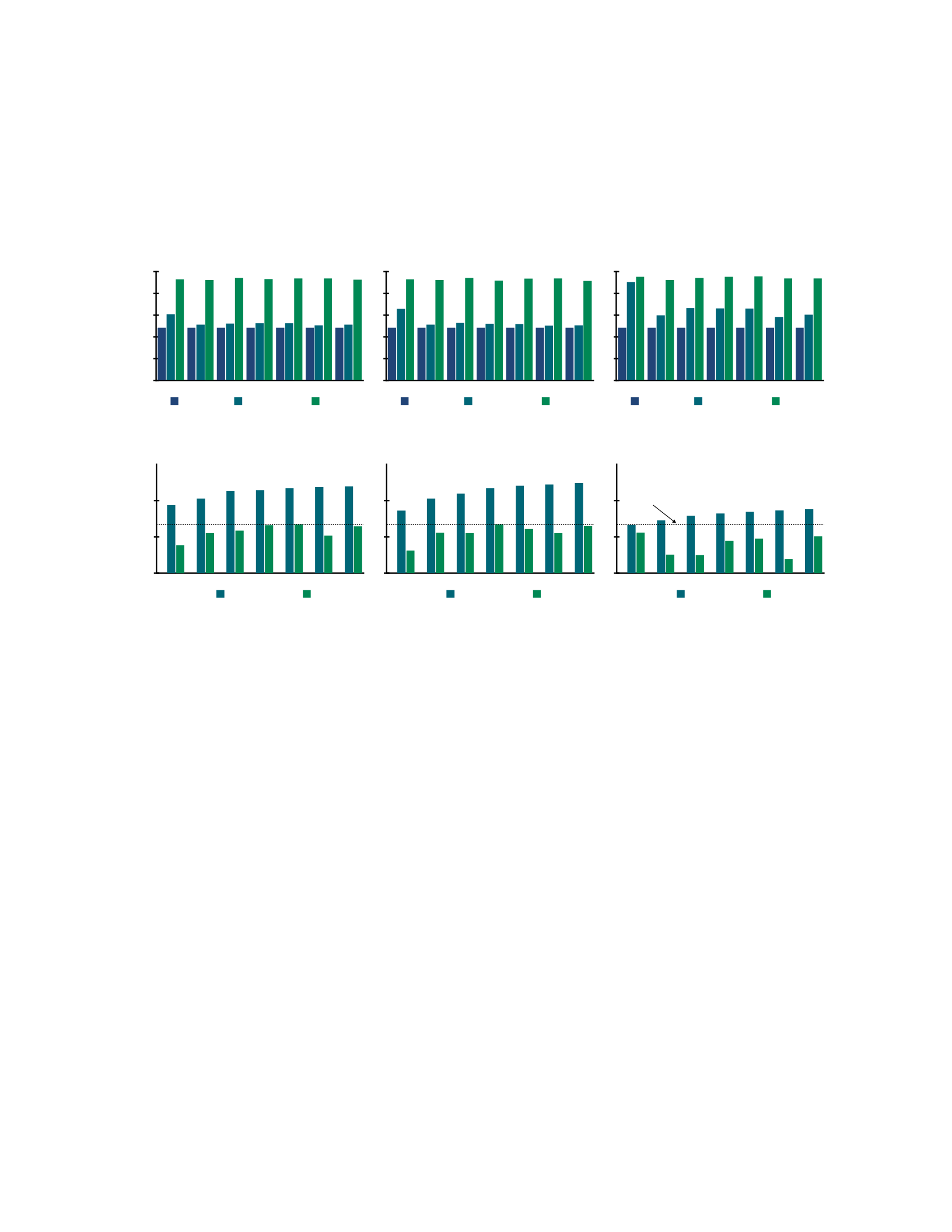
CHAPTER 4. MACHINE INFERENCE IN SPACE 39
4.4 Evaluation
This evaluation shows that, compared to directly deploying an application to a satellite or using a bent pipe, Kodan
consistently and significantly improves downlink data value density across applications and hardware platforms. A
key consequence of this improvement is up to a 12× reduction in satellite count to
Figure 4.8: Kodan improves data value density compared to the bent-pipe and direct-deploy baselines.
Figure 4.9: Kodan reduces processing time per frame by splitting each frame into fewer, larger tiles and eliding
processing of tiles sorted into high-value or low-value contexts. Note the y-axis log scale.
achieve full ground track coverage. These results also provide guidance to computer architects by showing the
computational capability required to meet the demands of different applications. After presenting these main
results, this work then focuses on the individual performance improvements of each technique leveraged by
Kodan. These techniques provide different benefits in different scenarios; geospatial contexts improve accuracy
and precision, while both frame tiling and context-based elision balance precision and execution time. By
intelligently selecting among these techniques for each application and hardware target, Kodan improves the
downlink data value density across scenarios.
4.4.1 Kodan Improves Data Value Density
Kodan improves data value density substantially for all applications on all hardware platforms compared to a bent-
pipe baseline and to a direct deployment of each application without Kodan, as shown in Figure 4.8. Compared to
the bent-pipe baseline, Kodan improves downlink data value density between 89 and 97 percent across all
applications and hardware platforms. For the bent-pipe baseline, the data value density depends solely on the
prevalence of high-value data because the satellite attempts to transmit all samples to the ground. In the direct
Deployment to Orin 15W
Data Value Density
0.0
0.2
0.4
0.6
0.8
1.0
App 1 App 2 App 3 App 4 App 5 App 6 App 7
Bent Pipe Direct Deploy Kodan
Deployment to i7-7800
0.0
0.2
0.4
0.6
0.8
1.0
App 1 App 2 App 3 App 4 App 5 App 6 App 7
Bent Pipe Direct Deploy Kodan
Deployment to 1070 Ti
0.0
0.2
0.4
0.6
0.8
1.0
App 1 App 2 App 3 App 4 App 5 App 6 App 7
Bent Pipe Direct Deploy Kodan
Deployment to 1070 Ti
1
10
100
App 1 App 2 App 3 App 4 App 5 App 6 App 7
Direct Deploy Kodan
Deployment to i7-7800
1
10
100
App 1 App 2 App 3 App 4 App 5 App 6 App 7
Direct Deploy Kodan
Deployment to Orin 15W
Time per Frame (s)
1
10
100
App 1 App 2 App 3 App 4 App 5 App 6 App 7
Direct Deploy Kodan
Frame deadline
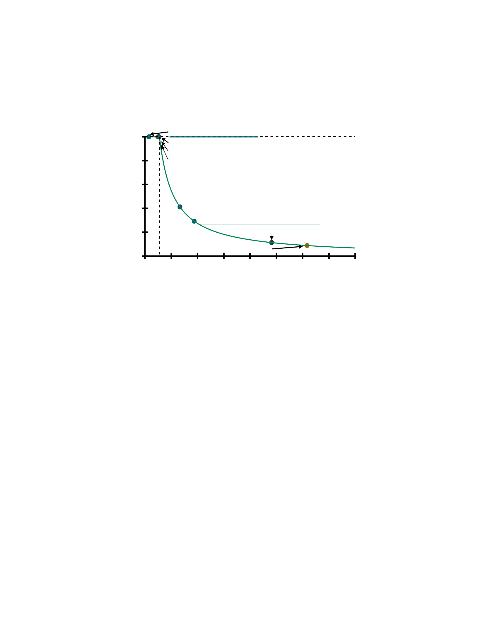
CHAPTER 4. MACHINE INFERENCE IN SPACE 40
deployment case, this work highlights two operating scenarios that illustrate the benefits of Kodan. In the first
scenario, an application is not computationally-constrained and processes each frame within the satellite data
sampling deadline. For these cases, the improvements under Kodan derive from use of geospatial contexts and
context-aware model specialization to improve
DVD vs.
Hardware Performance
1.0
0.8
0.6
0.4
0.2
0.0
Application Execution Time per Frame (s)
Figure 4.10: Each application and hardware pair exhibits a maximum data value density (DVD). Applications
meeting the frame deadline achieve this maximum DVD. As application execution time increases, DVD approaches
that of the bent pipe.
application accuracy and precision. In the second scenario, an application is computationally-constrained and fails
to process an entire frame within the satellite data sampling deadline. For these cases, the improvements under
Kodan derive from trading between precision and execution time via frame tiling and context-based elision of tile
processing. Figure 4.9 illustrates both of these scenarios.
0 40 80 120 160 200 240 280 320
App 1 Direct Deploy (Orin 15W)
App 1 Kodan (Orin 15W)
App 4 Direct Deploy (Orin 15W)
App 4 Kodan (Orin 15W)
App 7 Direct Deploy (Orin 15W)
App 7 Kodan (Orin 15W)
App 1 Direct Deploy (i7-7800)
App 1 Direct Deploy (1070 Ti)
Deadline
Per-App Maximum DVD
DVD, % Improved over
Bent Pipe (Norm. to Max.)
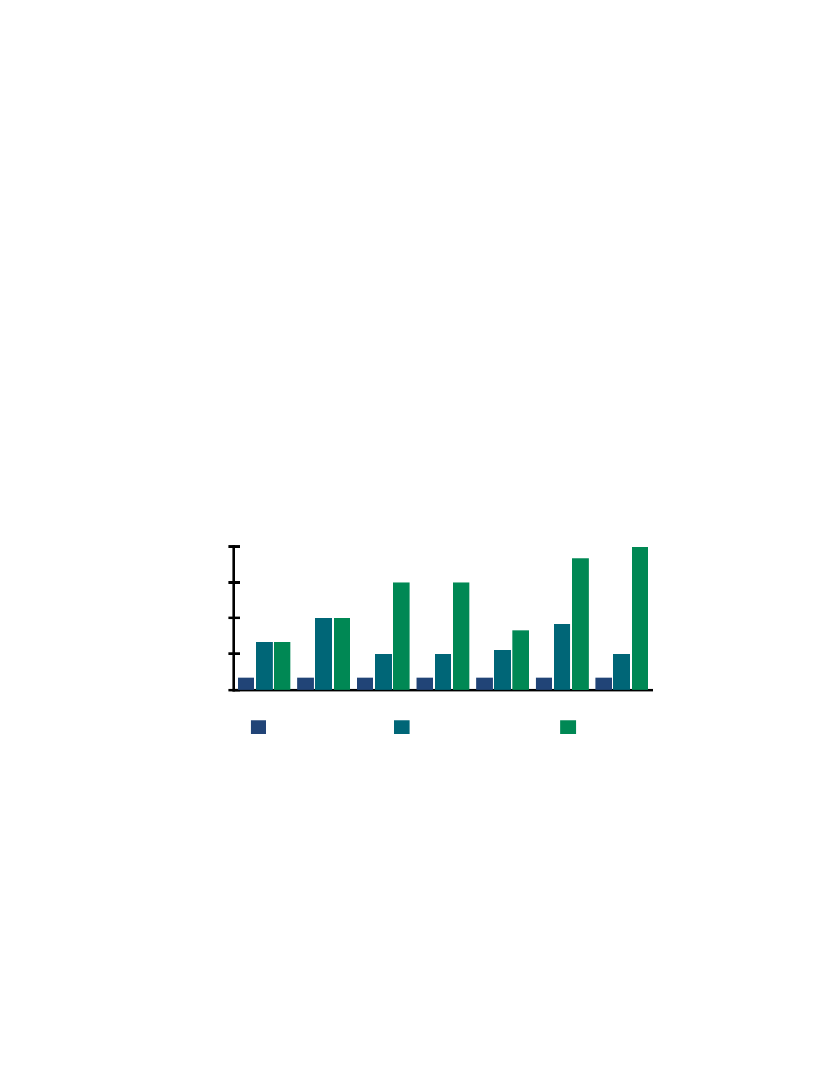
CHAPTER 4. MACHINE INFERENCE IN SPACE 41
The data reveal several important trends. The most constrained hardware platform (the Orin operating in a 15
W mode) exhibits the greatest improvement, illustrating the benefit of trading between precision and execution
time. The benefit reduces on the i7 because the applications are less computationallyconstrained than on the Orin
platform. On the 1070 Ti, where computational contraints are alleviated even more, the maximum precision
parameter selection often maximizes data value density.
4.4.2 Kodan Improves Satellite Performance
Kodan reduces the required per-satellite processing capability to support the applications evaluated, illuminating
specific compute performance requirements for continuous ground track processing coverage. Recall that, for
continuous ground track processing coverage, a satellite must process all tiles within the frame deadline. The bent
pipe model provides a baseline data value density by indiscriminately transmitting observations until saturating the
downlink. For each application, the maximum data value density depends on the highest precision the application
achieves within the frame deadline.
Figure 4.10 evaluates the relationship between frame processing time (i.e., compute performance) and
Fewer Satellites Provide Full Coverage
Figure 4.11: Using Kodan, the number of satellites in a constellation required for full ground track coverage reduces
up to 12× compared to directly deploying an application to the space edge and leveraging OEC techniques in prior
work [53].
improvement in data value density compared to the bent pipe minimum. The plot shows that reducing frame
processing time improves data value density until the time to process all tiles is less than the frame deadline. Once
frame processing time drops below the deadline, the downlink data value density of an application is limited by its
precision.
Reduction Factor
0
3
6
9
12
App 1 App 2 App 3 App 4 App 5 App 6 App 7
Direct Deploy Max. Prec. Tiling Kodan
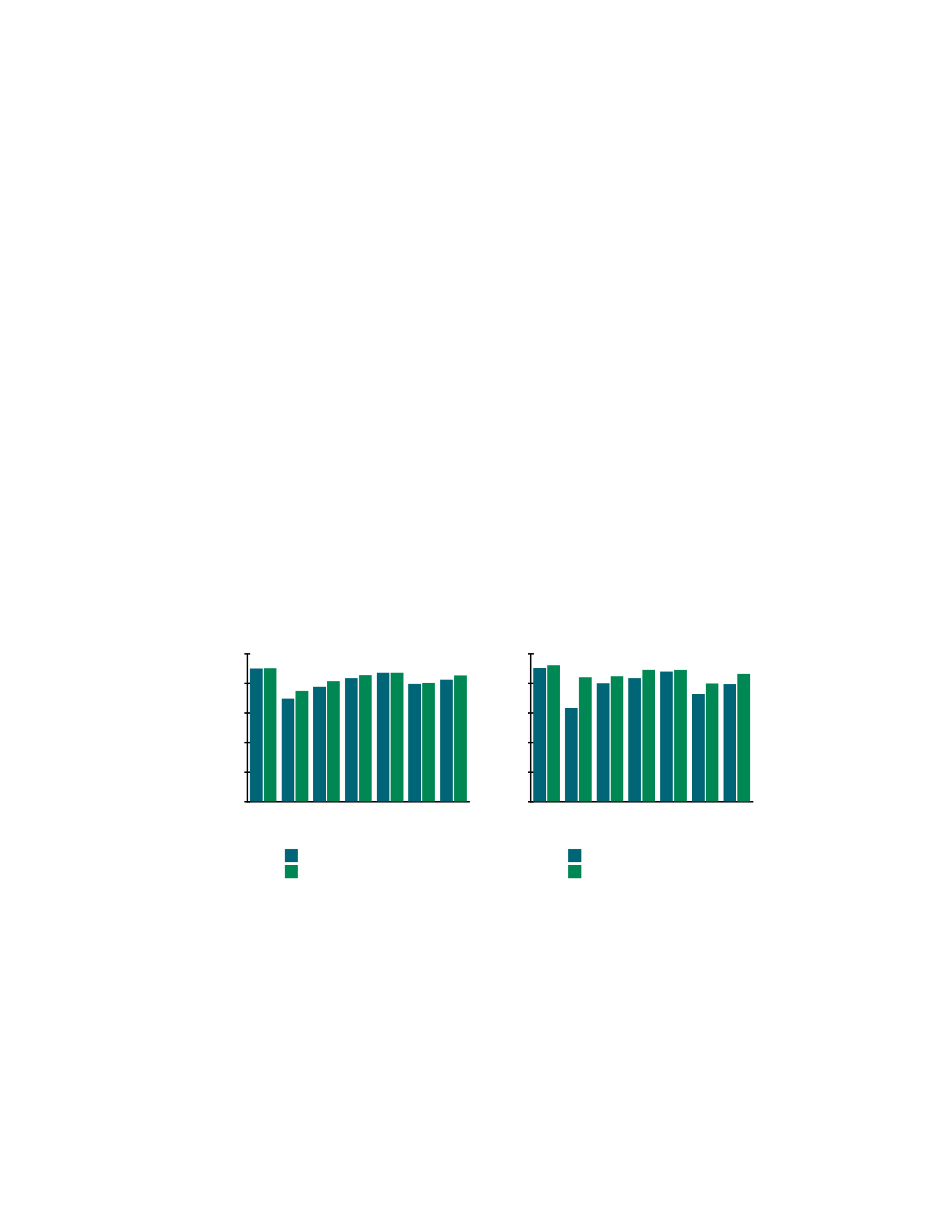
CHAPTER 4. MACHINE INFERENCE IN SPACE 42
Points in the plot are measured data value densities for different application/hardware combinations from the
evaluation. These points show Kodan improves data value density for Applications 1, 4, and 7, especially when
exceeding the frame deadline when directly deployed to the hardware targets. Each application consists of a
different number of operations, and therefore they require different amounts of time to complete; Application 1
consists of the fewest number of operations and Application 7 consists of the most. Application 1 directly deployed
to the 1070 Ti meets the deadline; thus, the downlink data value density depends only on the application precision
(see Figure 4.8 for the effects of precision differences between direct deploy and Kodan on data value density).
When directly deployed to the i7 or to the Orin, Application 1 falls short of the maximum data value density
because it executes too slowly to meet the deadline. Using Kodan, Application 1 executes significantly faster. The
resulting idle time affords Kodan the opportunity to deploy models of higher precision to improve data value
density.
Directly deploying Application 4 or Application 7 to the Orin gives worse results. Using Kodan, both applications
attain their maximum achievable data value density due to significant reductions in execution time. Future
satellites — especially nanosatellites — are likely to include hardware similar to the Orin due to its low power
consumption. Rather than directly deploying to such a device, using Kodan alleviates the computational bottleneck,
which exists even for the simplest of the benchmark applications. Figure 4.11
Figure 4.12: Left: Contexts improve accuracy (fraction of labels correct). Right: When an application meets the frame
deadline, increasing precision using contexts benefits data value density.
Geospatial Contexts and Accuracy
Fraction Correct
0.0
0.2
0.4
0.6
0.8
1.0
App 1
App 2
App 3
App 4
App 5
App 6
App 7
Direct Deploy
Geospatial Contexts
Geospatial Contexts and Precision
Precision: TP/(TP+FP)
0.0
0.2
0.4
0.6
0.8
1.0
App 1
App 2
App 3
App 4
App 5
App 6
App 7
Direct Deploy
Geospatial Contexts
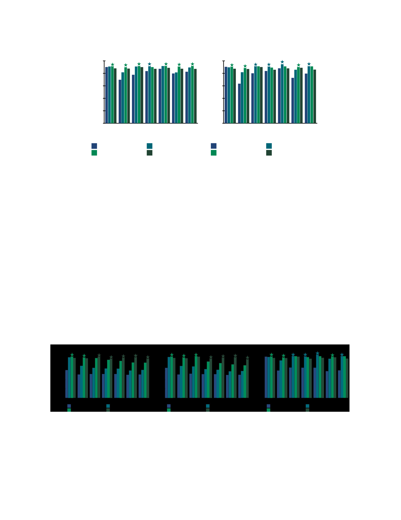
CHAPTER 4. MACHINE INFERENCE IN SPACE 43
Figure 4.13: Left: The accuracy-maximal tiling varies by application. Right: Tiling varies precision. Absent a
computational bottleneck, maximizing precision maximizes data value density.
shows that Kodan reduces satellite count for full ground track coverage up to 12× compared to directly deploying an
application to the space edge with OEC techniques in prior work [53].
4.4.3 Contexts Improve Precision
Kodan uses geospatial contexts to improve both accuracy and precision for all applications, garnering a data value
density benefit regardless of whether the satellite experiences a computational bottleneck. With a saturated
downlink, precision — here, the fraction of correctly labeled pixels — determines data value density, because
incorrectly-labeled pixels “pollute” the already-saturated downlink. Figure 4.12, right, displays the effect of context-
specific model selection on application precision. The increase in application precision with geospatial contexts is
more pronounced than the increase in application accuracy. For example, Application 2 improves in precision by
33% with geospatial contexts. Figure 4.12, left, shows
Figure 4.14: On more computationally-constrained platforms like the Orin, more aggressive tiling (nine per frame)
maximizes data value density. As the computational bottleneck eases (1070 Ti) tilings that maximize precision also
maximize data value density.
Effect of Tiling on Accuracy
Fraction Correct
0.0
0.2
0.4
0.6
0.8
1.0
App 1
App 2
App 3
App 4
App 5
App 6
App 7
Tiles/Frame121 Tiles/Frame36
16 Tiles/Frame Tiles/Frame9
Effect of Tiling on Precision
Precision: TP/(TP+FP)
0.0
0.2
0.4
0.6
0.8
1.0
App 1
App 2
App 3
App 4
App 5
App 6
App 7
121 Tiles/Frame 36 Tiles/Frame
16 Tiles/Frame 9 Tiles/Frame
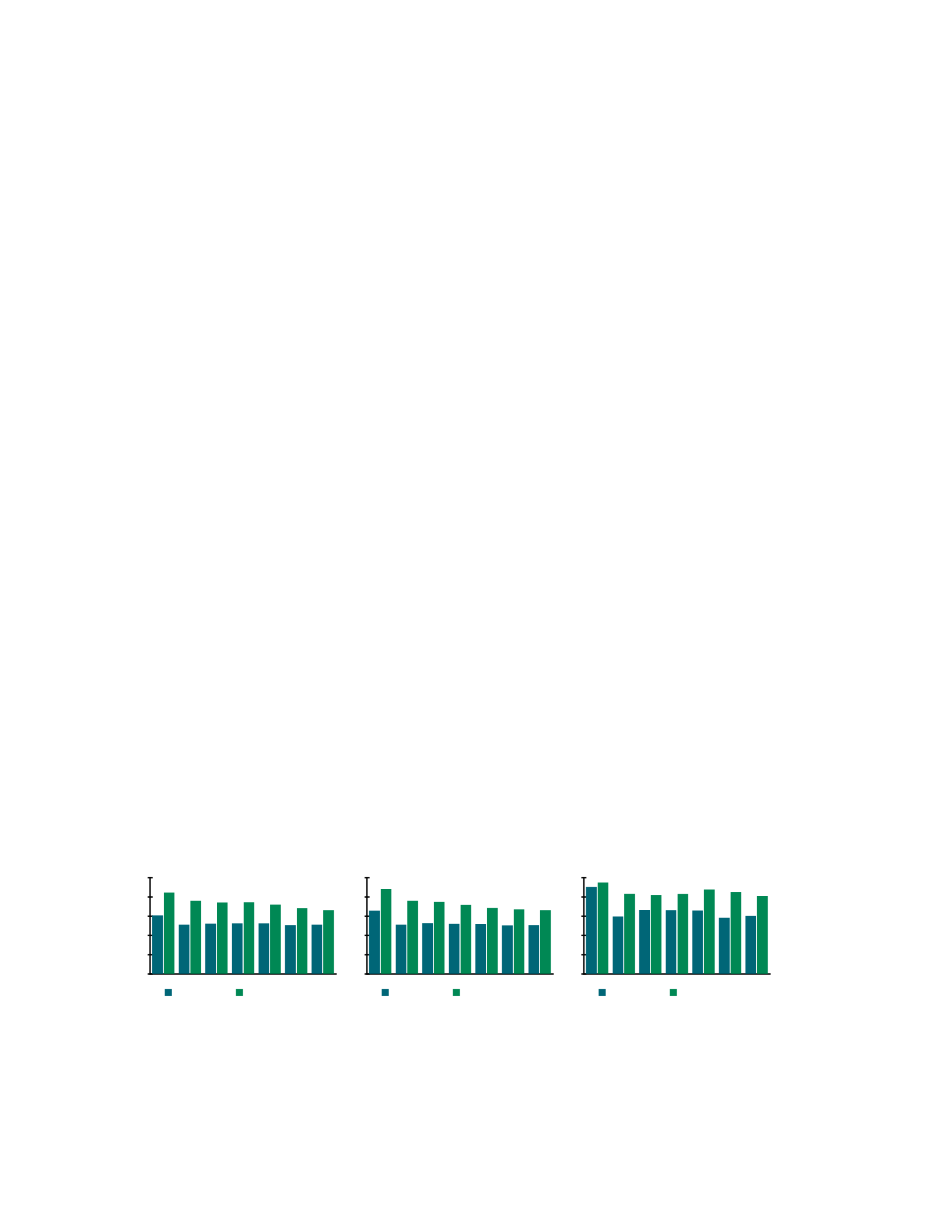
CHAPTER 4. MACHINE INFERENCE IN SPACE 44
that context-specific model selection also improves accuracy by up to 7.5%. Applications with the lowest baseline
accuracy experience the greatest improvement (e.g., Application 2).
4.4.4 Tiling Trades Precision and Performance
Kodan uses frame tiling to improve data value density by adjusting tile count per frame to balance frame processing
time with application precision. Figure 4.13, left, shows how tiling affects application accuracy. Figure 4.13, right,
displays the effect of tiling on application precision. Each application has a tile count that maximizes accuracy and a
tile count that maximizes precision. Increasing or decreasing tile count from these optimal tilings decreases
accuracy or precision; this finding is consistent with prior work [52].
Absent a computational bottleneck, the maximum precision tiling yields the maximum data value density.
When computationally bottlenecked, Kodan selects a tiling to reduce execution time at the expense of precision
in order to increase data value density. Figure 4.14 illustrates this effect. Tiling provides up to a 50% improvement
in data value density for the most computationally-constrained platform and the most computationally-costly
application (i.e., Application 7 on the Orin mobile GPU). To understand this result, recall that processing more data
provides substantial data value density improvements until meeting the frame deadline, when precisely processing
tiles becomes most important (see Figure 4.10). For simpler applications (e.g., Application 1) and more capable
platforms (e.g., the 1070 Ti), less aggressive tiling supports higher precision within the frame deadline.
4.4.5 Elision Improves Data Value Density
Kodan uses context-based elision to downlink or discard samples from primarily high-value or lowvalue contexts
and thereby substantially increases data value density. Figure 4.15 illustrates this effect. Improvements from elision
are more pronounced under a greater computational bottleneck; for example, when Application 7 deploys to the
Orin. As the computational bottleneck eases (e.g., simpler applications
Figure 4.15: Some contexts consist mostly of high-value or low-value data. Downlinking samples from high-value
contexts and discarding samples from low-value contexts — i.e., eliding further processing — eases the
computational bottleneck by freeing time to filter samples from other contexts.
Context-Based Elision & Data Value Density (Orin 15W)
High-Value Downlink Fraction
0.0
0.2
0.4
0.6
0.8
1.0
App 1 App 2 App 3 App 4 App 5 App 6 App 7
Direct Deploy Context-Based Elision
Context-Based Elision and Data Value Density (i7-7800)
High-Value Downlink Fraction
0.0
0.2
0.4
0.6
0.8
1.0
App 1 App 2 App 3 App 4 App 5 App 6 App 7
Direct Deploy Context-Based Elision
Context-Based Elision and Data Value Density (1070 Ti)
High-Value Downlink Fraction
0.0
0.2
0.4
0.6
0.8
1.0
App 1 App 2 App 3 App 4 App 5 App 6 App 7
Direct Deploy Context-Based Elision

CHAPTER 4. MACHINE INFERENCE IN SPACE 45
or better hardware), the benefit of elision becomes less pronounced because the system processes more samples
within the deadline. For example, the data value density improvement for Application 1 is 39% on the Orin
platform, while the data value density improvement for Application 1 is 34% on the i7 platform. On the 1070 Ti
platform, Application 1 is not computationally bottlenecked; instead, the benefits derive from the precision
improvement of sending down likely high-value pixels without processing, rather than imprecisely processing those
pixels and transmitting a worse result.
4.5 Related Work
This work spans computer systems, space systems, space networks, and systems ML. Section 4.1 provides an
overview of the emerging computational space systems domain, and Section 4.1.1 characterizes major challenges
of this research area. Recent works in orbital edge computing provide context for this work. The space networking
challenge of the bent pipe bottleneck is quantified in [52], which also introduces the concept of a computational
satellite deploying machine inference to address this challenge. Orbital edge computing [53] aims to address the
downlink bottleneck and introduces the computational bottleneck of the inelastic space edge. Challenges and
opportunities in this domain are examined in [148].
The computational bottleneck poses a major space systems challenge. Although monolithic satellites cost
hundreds of millions of US dollars each, this high cost does not provide high-performance onboard processors.
These systems must operate for decades to justify the high cost, which means that computer hardware must be
low-risk and highly-reliable. Often, these systems use decades-old, “flight heritage” CPUs. After two or more
decades of operation, onboard processors could be nearly half a century behind
the state-of-the-art.
For example, LEON processors — which receive significant support from the European Space Agency (ESA) —
implement the 32-bit SPARC V8 instruction set architecture (ISA). A recent implementation achieved a clock
frequency of 250 MHz [6]. The EO-1 makes use of a 12 MHz Mongoose-V central processing unit (CPU), which
implements the 32-bit MIPS ISA, to demonstrate autonomous science [38]. The RAD5500 implements a 64-bit
PowerPC ISA operating at 466 MHz [19]. The limited performance of these CPUs stems from larger technology
nodes and functional unit duplication, which help to provide reliability in the space environment. Extremely high
costs demand extremely low risk and long-duration missions at the expense of performance. Recent trends in
space systems have started to consider COTS embedded computer systems [145, 146].
Several works consider models optimized for accuracy or speed in terrestrial applications [219, 123, 103, 172,
262, 27]. Works on embedded, terrestrial, wireless sensor systems study the tradeoff between computation and

CHAPTER 4. MACHINE INFERENCE IN SPACE 46
communication for energy-harvesting devices [60, 59, 174, 83, 81]. These works identify the relatively high energy
cost of communication and quantify benefits to spending energy on computation instead. While these terrestrial
systems can transmit data at any time within energy constraints, satellites can transmit data only while near a
ground station. This work focuses on model specialization for geospatial contexts at the orbital edge to improve the
data value density of a saturated downlink.
Space networking is a growing field of research [128, 88, 21]. Much work focuses on inter-satellite
communication, which is a challenging engineering question encompassing control theory, orbital dynamics,
robotics, and energy-performance tradeoffs. Less attention has been paid to the challenges of the downlink
bottleneck and the saturated downlink, which are examined in this work. Alternate approaches to addressing the
downlink bottleneck [247] are complementary to this work by enabling higher performance with even smaller
satellite constellation populations.
4.6 Summary
The increasing accessibility of space opens the orbital edge to new geospatial analysis applications. A limited
downlink creates a need for on-orbit processing to extract value from sensor data. However, constraints on orbital
edge computing limit the value of satellite-based applications. Kodan mitigates the downlink bottleneck and the
computational bottleneck for space edge systems by leveraging geospatial contexts and specializing satellite
computation to balance application processing time with precision. This approach contrasts with expensive,
constellation-oriented techniques that extract value from data but require many satellites to do so. This work
implements and evaluates Kodan, which increases the density of valuable data downlinked from LEO between 89
and 97 percent without changing ground infrastructure or radio attributes despite bottlenecked bandwidth and
computing.
Orbital edge computing has an exciting future with many open research questions. Building on this work,
computational space system designers should improve sensor coverage and computing capability of constellations
through co-design of system-level optimizations and computer architecture while avoiding unfavorable cost-scaling
of high device counts. Future constellations will feature heterogeneous sensors, computational capabilities, and
actuators. Some satellites may share data via crosslinks and distribute processing so that each satellite need not
contain telescope optics, precision pointing, laser communication, and a high-end GPU. Instead, a heterogeneous
constellation supports hardware specialization (as opposed to processing specialization based on sample context),
allowing individual satellites to contain fewer subsystems are therefore be more simple. Energy constraints, orbital
dynamics, and client mission goals place time-dependent constraints on satellite operations. Communication and

CHAPTER 4. MACHINE INFERENCE IN SPACE 47
computation will remain perennial challenges for space-based computer systems. Kodan demonstrates that these
challenges are surmountable with new techniques tailored to the unique constraints of the orbital edge.

Chapter 5
Nanosatellite Constellation Design
A resurgence in the space industry [64, 257, 162, 30], concurrent with standardization of nanosatellite form factors
[167] and a declining cost of access to space [78], has stimulated an exponential growth in nanosatellite launches
over the past two decades [224]. The largest commercial satellite constellations today consist of hundreds of Earth-
observing, camera-equipped nanosatellites [29, 138], each measuring centimeters, massing a few kilograms, and
costing only thousands of USD. These emerging systems are a stark contrast to the extremely expensive, monolithic
space vehicles of the past. For example, the $192,000,000, 500 kg Earth Observing-1 (EO-1) is a “one-of-a-kind”
[168] satellite operating for 16 years under a NASA ground control team. This single-satellite remote sensing
mission depended on NASA’s extensive ground infrastructure to support its communication model: operators
manually schedule communication on ground stations shared among all other space missions. The EO-1 mission
terminated when its ground support was de-funded, leaving no one to schedule communication and data
management operations. As nanosatellites proliferate, the viability of building and operating a manual, bent-pipe
system architecture diminishes. The scale of this challenge is increasing; several commercial ventures have
announced plans to deploy satellite constellations consisting of thousands of devices over the next ten years [89,
196, 197, 96, 97, 98, 226, 228, 227].
A trend toward massive constellations of low Earth orbit (LEO) nanosatellites demands a new architecture for
space systems. As with large, expensive space vehicles of the past, nanosatellite constellations today still rely on a
communication model that sends remote control commands to orbit and delivers sensed data to Earth [61]; this
design is referred to as a “bent pipe” by space system architects [136]. Momentum towards large constellations of
nanosatellites requires a reimagining of space systems as distributed, edge-sensing and edge-computing systems.
As work on warehouse scale computing [16] did for datacenters-as-computers, this work aims to raise awareness of
system-level research questions for orbital
50
edge computer systems equipped with high-datarate cameras and sensors. This work characterizes and addresses
computer hardware and software design challenges for orbital edge computer systems, many of which stem from
physical deployment constraints and limitations inherent to ground infrastructure.

CHAPTER 5. NANOSATELLITE CONSTELLATION DESIGN 49
Addressing the challenges of the orbital edge is a timely and important problem due to the recent proliferation
of nanosatellite systems. Space system architects are eschewing large, costly (e.g. $650,000,000 [74]), “exquisite”
[231] satellites for constellations of small, inexpensive (e.g. $65,000 ea.) “CubeSats” [167]. Commercial efforts
[138, 29] use this 10,000× lower per-device cost to deploy large, sensor-equipped nanosatellite constellations to
LEO and observe the planet with high temporal resolution. Such systems create new capabilities for precision
agriculture, environmental and infrastructure monitoring, humanitarian assistance and disaster relief, security,
climate, and other commercial uses.
Challenges faced by existing systems under a bent-pipe architecture stem from fundamental physical
constraints. The time-varying relationship between the geographic location of ground stations and the orbital
position of nanosatellites imposes limitations on link availability and can lead to high downlink latencies.
Intermittently available downlinks incur high latency between data collection and data processing in existing
systems that simply downlink raw observations. Downlinks can be unreliable; one nanosatellite mission reports
88% packet loss [176]. Commercial ventures require complex, custom downlink solutions [61]. Shared “last mile”
infrastructures [259, 5] aid availability but do not address the terrestrial centralization bottleneck. Limits on
downlink bitrate prevent bent pipes from scaling to accommodate the extreme data volumes of large constellations
and create a need for a new system architecture less reliant on communication.
On Earth, sensor systems increasingly leverage edge computing by performing sensor-local data processing in
lieu of communication to a cloud datacenter [205]. While access to the cloud from the edge can accelerate
computing [24], any benefits depend on backhaul network availability. High-datarate sensors deployed across large
geographic environments face a network bottleneck from the sensor to the datacenter as datarate exceeds
bandwidth [205, 100]. Processing data at the edge avoids high-bitrate infrastructure at each sensor and supports a
larger population of deployed devices. Edge processing avoids the privacy and security risks of multi-tenant
infrastructures in shared datacenters [132, 140, 70].
Applying these terrestrial edge computing techniques directly to space systems is appealing, but nanosatellite
constellations are subject to a unique set of operating constraints that typically do not affect terrestrial edge
systems. In space, unlike on Earth, all energy for computation and communication must be harvested from the
environment — plugging into a power grid is not an option. The small size of a nanosatellite, which is dictated by
the cubesat standard, limits solar panel surface area and thus limits power. Unlike on Earth, the quality of visual
data in space is fundamentally limited not only by onboard sensors, but also by chassis size (which limits focal
length) and orbit altitude (which limits optical resolution). Communication bitrate, which is affected by orbit
parameters, ground station capability, and ground station location, dictates the amount of data satellites buffer

CHAPTER 5. NANOSATELLITE CONSTELLATION DESIGN 50
between downlinks. Any viable orbital edge computer system must directly address these unique physical
constraints.
This work proposes Orbital Edge Computing (OEC) as an alternative to existing nanosatellite constellation bent-
pipe architectures. OEC colocates processing hardware with high-datarate spectral sensors in small, low-cost
satellites. This work characterizes the physically-constrained design space of a computational nanosatellite,
revealing fundamental limitations on data quality and computation inherent to state-of-the-art designs. Based on
this design space study, this work introduces computational nanosatellite pipelines (CNPs) as an organizational
principle for OEC constellations. A CNP distributes sensing, processing, and communication across a constellation in
order to remain within latency and energy envelopes.
This work then develops cote1, the first orbital edge computing simulator (cote-sim) and runtime service (cote-
lib). cote physically models orbital mechanics and Earth rotation to track ground station and satellite positions over
time. cote models data collection along each satellite ground track, as well as the energy and latency of sensing,
computing, and communication for an entire constellation. cote is useful for mission design and simulation (cote-
sim) and as an online runtime service for each nanosatellite and ground station (cote-lib).
This work uses cote-sim to quantitatively demonstrate the limitations of bent pipes, the advantages of OEC, and
the benefits of nanosatellite pipelines. cote-lib runs on each device and provides continuous access to a physics-
based model of the constellation and ground infrastructure in order to enable autonomy. By directly modeling the
physics of the system, each satellite determines at runtime when to downlink, when to process locally, and how to
distribute responsibilities across a pipeline without the need for online coordination or cross-link communication.
cote-lib enables OEC by eliminating the reliance on
remote control through a bent pipe.
In summary, this chapter presents the following contributions: (i) a demonstration of the limitations of bent
pipes using a novel, physics-based simulator that includes orbital dynamics, communication, energy harvesting,
and data collection; an OEC architecture can reduce ground station infrastructure over 24× compared to a bent-
pipe architecture; (ii) a characterization of the physical design space of an OEC device and an identification of key
limitations that drive constellation design; (iii) a proposal and evaluation of computational nanosatellite pipelines:
an organizational principle for OEC constellations that distributes work across devices; CNPs can reduce system
edge processing latency over 617×; and (iv) a runtime service deployed to each nanosatellite and ground station
that models the constellation, ground
abundant energy, high cost limited energy, low cost
Figure 5.1: A comparison between a monolithic satellite and a nanosatellite. This work proposes augmenting
existing systems by incorporating onboard visual processing components.
1 Computing on the edge. A cote is a shelter for carrier pigeons.

CHAPTER 5. NANOSATELLITE CONSTELLATION DESIGN 51
infrastructure, and energy environment in order to autonomously schedule sensing, communication, and
computing without the need for cross-link coordination.
5.1 Background on Nanosatellite Constellations
Momentum away from exquisite [231], monolithic satellites towards small, cheap nanosatellites reduces the cost
of remote sensing in space by orders of magnitude. A nanosatellite has a mass between 1 kg and 10 kg, often
adhering to the “CubeSat” standard [167] to enable use of commercial, off-the-shelf (COTS) components and avoid
custom deployers [184]. A cubesat is physically constrained to 10 cm×10 cm×10 cm (“1U”) volumes, with mass
limited to 1.33 kg per 1U. This volume must house all sensors, actuators, and communication subsystems.
Computers onboard existing nanosatellites are simple, low-performance systems for command and data handling
(C&DH), guidance navigation and control (GNC), buffering sensor data, and communication. Virtually all
nanosatellites today rely on a ground control segment to manage data.
A nanosatellite electrical power system (EPS) collects, stores, and distributes energy. Many low-cost cubesats
avoid higher-risk, deployable solar arrays and instead rely on surface-mounted solar panels. As a result, the small
size of the satellite constrains collected power to a few watts. Batteries must be small due to limited cubesat
volume and mass. To prevent damage, batteries are heated in the cold of space (e.g. -40 ◦C), incurring a power cost
overhead [71]. Supercapacitor storage is less energy-dense, but has less mass, less volume, and avoids thermal
issues; this work focuses on supercapacitor energy storage.
Figure 5.1 illustrates the magnitude of the shift from large, monolithic satellites to nanosatellites. Monolithic
satellites are meters in size, thousands of kilograms in mass, collect kilowatts of power, and can cost over half a
billion USD [62]. A nanosatellite is four orders of magnitude smaller (cubic centimeters), has three orders of
magnitude less mass (a few kilograms), collects three orders of magnitude less power (a few watts), and has four
orders of magnitude lower cost.
A nanosatellite constellation is a collection of nanosatellites that share a purpose. Existing nanosatellite
constellations are coordinated from the ground, often to accomplish a remote sensing task (e.g. imaging the Earth).
Today, commercial ventures leverage the relatively low per-device cost of nanosatellites to operate large
constellations [29, 138]. In the future, public and private organizations expect to launch constellations of thousands
of devices, each with high-datarate sensors and the capacity for more capable onboard computers.
A constellation consists of a ground segment and a space segment. In bent-pipe architectures, the ground
segment consists of geographically-distributed, manually-controlled transceivers, and the space segment consists
of remote-controlled satellites in one or more orbits. As shown quantitatively in Section 5.2.3 and Section 5.6.1,
bent pipes break down as the amount of edge-sensed data increases. Further, limited link availability and bitrate

CHAPTER 5. NANOSATELLITE CONSTELLATION DESIGN 52
bottlenecks can cause reconfiguration of a constellation to take days, weeks, or months [63]. These growing
limitations of bent-pipe architectures motivate the OEC techniques presented in this work.
5.2 Challenges of Computational Nanosatellites
Computational nanosatellite architects face three key challenges. First, physical constraints on nanosatellite design
(e.g. orbit altitude or volume limitations imposed by the cubesat standard) bound the achievable fidelity of visual
data. Second, orbit characteristics determine data collection rate because satellite position and velocity dictate
when and how often to capture data. Third, the relationship between orbit characteristics, Earth rotation, and
ground station locations determines downlink availability, duration, and bitrate.
5.2.1 Data Quality is Physically Constrained
The physical design of a nanosatellite limits visual sensor data quality. Satellite image quality is measured by
ground sample distance (GSD), i.e. the geographic distance represented between centers of adjacent
1.5U Camera Volume 2.0U Camera Volume 2.5U Camera Volume
Figure 5.2: A 3U cubesat camera design space, assuming the smallest commercially available pixel sensor size (1.1
um)
pixels. As GSD decreases, image quality increases. Commercial, monolithic systems have GSD as low as 0.3 m/px
[62], while commercial nanosatellite systems have GSD around 3.0 m/px [180].
Three parameters govern GSD: orbit altitude, camera focal length, and pixel sensor size. Merit is proportional to
focal length and inversely proportional to altitude and sensor size.
Sensor size. This work assumes a COTS image sensor of at least 4096 × 3072 pixel sensors (i.e. 4K), each 1.1 µm
[178] in size.
Orbit altitude. Orbit altitude is often between 325 km and 825 km for LEO. Higher altitudes support longer
missions (years instead of weeks), but suffer worse image quality.
Focal length. The cubesat standard bounds camera focal length because components compete for limited
volume. Earth-observation cubesats must include radios, energy storage, computing systems, and an attitude
determination and control system (ADACS) to point the camera.
Designing for Low GSD. An Earth-observing satellite should optimize for low GSD. Figure 5.2 plots a cubesat design
space, assuming a 3U volume (like existing, commercial systems [61]) and calculating GSDs with the pinhole camera
model [90]. Each curve represents a different camera focal length. The data show that a 20 cm focal length
provides a GSD of 2.26 m/px, which is 7.5× worse than a monolithic satellite but comparable to existing cubesats.
CHAPTER 5. NANOSATELLITE CONSTELLATION DESIGN 53
Low GSD requires a long focal length, limiting non-camera components to a 1U volume. Figure 5.3 charts
contributions of state-of-the-art nanosatellite subsystems
[2,
10
5
0 0
ADACSCamera System
C&DHComm. System
Figure 5.3: The volume, mass, power, and cost of an Earth-observing, 3U cubesat. These nanosatellites are
constrained in volume and power, but not in mass or cost.
213, 107, 112, 71, 67, 105, 104, 106, 11] toward volume, mass, power, and cost, revealing that volume and power
limit cubesat design while mass and cost do not.
5.2.2 Data Rate Depends on Orbit Parameters
The astrodynamics of a nanosatellite determine the optimal rate at which to collect images. This rate must be both
frequent enough to cover the entire ground track, and infrequent enough to avoid redundant data. A satellite
avoids collecting redundant images by making observations at the ground track frame rate (GTFR). The GTFR is the
rate at which an entirely new geographic scene fills the camera view with no pixel overlapping a previous frame.
The ground track frame period (GTFP) is the inverse of GTFR, i.e. the time a nanosatellite takes to pass over one
ground track frame. To minimize data volume, camera sensors need not capture frames at rates higher than the
GTFR. In order to achieve sufficient coverage of a ground track, a satellite or constellation must capture images
individually or in aggregate at the GTFR.
Section 5.3.2 discusses distributing sensing across a constellation.
5.2.3 Bitrate Bottlenecks Constrain Constellations
Bent pipes break as nanosatellite constellation population increases due to limitations on downlink availability and
bitrate. Under a bent-pipe architecture, each nanosatellite stores data (generally for minutes or hours) until it nears
a ground station. During a downlink session, which lasts between a few seconds and ten minutes, the satellite
Power
(W)
ADACS Camera System
Chassis C&DH
Comm. System Energy System
75
Solar Panels50
7.1
25
Cost
(%)

CHAPTER 5. NANOSATELLITE CONSTELLATION DESIGN 54
transmits its unprocessed data. Under this model, existing systems [61] experience a 5.5 h delay before data reach
customers. Reconfiguring a constellation via uplink takes longer; initial configuration lasts months [29].
Bent-pipe architectures require many ground stations to support a large constellation. This work evaluates
existing, bent-pipe constellations with cote-sim in Section 5.6.1 and provides a simple motivating example here. A
satellite in a polar orbit has access to all latitudes and, with a sun-synchronous orbit, ensures consistent pass times.
Such a satellite at a 410 km altitude has an orbit period of 92.9 min and revisits the same point on Earth every two
days [28]. Existing ground stations with a 200 Mbit/s downlink datarate [61] retrieve up to 15 GB of data per 10 min
session. With these parameters, a ground station optimistically and ideally positioned to observe every pass (e.g. a
polar station for a polar orbit) supports only 9 satellites per revolution. Supporting a future 1000-satellite
constellation requires 112 of these ideally positioned stations.
Provisioning this costly ground station network may be pointless, because a large fraction of downlinked images
contain no features of interest. And, as cote-sim reveals in Section 5.6.1, this estimate is overly ideal. It assumes
that satellites are positioned in orbit such that all 112 ground stations are constantly in use, and it assumes that all
satellites receive a full 10 min of downlink time. cote-sim reveals that neither of these assumptions hold true in
realistic systems.
OEC Eliminates the Bent-Pipe Bottleneck OEC reduces the need for a large number of ground stations by
processing images on orbit, downlinking only interesting images, and discarding or logging the rest. For example,
assuming that machine inference identifies 0.75 GB of interesting data out of 15 GB of raw data, all data downlink
in only 30 s at 200 Mbit/s. Instead of servicing just 9 satellites per revolution, each ground station supports 185
satellites, and a constellation of 1000 OEC satellites requires only 6 ground
stations.
5.3 Orbital Edge Computing
OEC is a nanosatellite system design consisting of a set of organizational principles that relies on nearsensor
processing in order to avoid the limitations of bent-pipe architectures. This section first provides an overview of an
individual OEC nanosatellite, i.e. a computational nanosatellite. It then describes a computational nanosatellite
pipeline (CNP), which organizes a constellation into a parallel pipeline to hide processing latency by leveraging
formation flying techniques [15, 151].
Figure 5.4: Top: The orbit determines the ground track, i.e. the locations over which a satellite passes. A ground
track can be separated into a sequence of ground track frames. Typically, each frame is tiled before processing.
Bottom: An illustration of a CNP. A satellite images a ground track frame and performs processing until arriving at
the next frame.

CHAPTER 5. NANOSATELLITE CONSTELLATION DESIGN 55
5.3.1 Computational Nanosatellites
A computational nanosatellite is a nanosatellite with several key changes to its computing hardware and power
system.
Computing Hardware. A computational nanosatellite supplements existing sensing, communication, and
control hardware with onboard computing. This work characterizes onboard computing with a Jetson TX2 industrial
module. The Jetson TX2 includes a high-capability, low-power, efficient mobile GPU; the industrial variant is
designed for extreme temperature environments. Its small volume allows for integration among all other necessary
components within the 1U volume available to a 3U cubesat containing a 2U camera system. A 7.5 W power mode
closely matches the 7.1 W input power provided by surface-mounted solar panels. The OEC computing model
supports computing systems other than the
Jetson by varying input performance and energy parameters.
Energy. A computational nanosatellite harvests and stores energy. In this work, the energy harvester is a low-
risk, chassis-mounted solar cell array that avoids the mechanical complexity of deployable panels. A chassis-
mounted array limits total solar cell area and, as a result, available power peaks at about 7.1 W. A high-density
supercapacitor bank stores energy. Supercapacitors hold less total energy than batteries of the same volume, but
offer several advantages. Supercapacitors charge quickly and provide immediate, high current; batteries charge
slowly and are current-limited. Supercapacitors operate across the wide range of temperatures in space, while
batteries fail in excessive heat or cold. OEC systems operate like intermittent systems [149, 44, 94, 241, 95, 154, 46,
263, 93], harvesting energy while sleeping to charge capacitors. When energy is sufficient, it performs its sensing,
computing, or communication task.
Operating Model. A computational nanosatellite operates by capturing an image and processing it locally
instead of transmitting it to Earth through a bent pipe. The application determines the processing method.
Examples include CNN-based image classification, object detection, and segmentation, or any other computation;
Section 5.6 evaluates OEC systems with onboard machine inference. A typical OEC processing task identifies
features of interest, separating them from raw sensor data. An OEC system discards uninteresting data and sends
processed features of interest to Earth, using intelligent early discard as described by prior work [52].
5.3.2 Computational Nanosatellite Pipelines
An OEC system is energy and latency constrained. While processing a frame, a nanosatellite can capture but not
process additional frames. A nanosatellite cannot capture a frame while sleeping. Effective OEC systems leverage
the constellation as a whole to overcome energy and latency constraints.

CHAPTER 5. NANOSATELLITE CONSTELLATION DESIGN 56
A constellation of OEC nanosatellites overcomes the energy and latency limitations of individual satellites by
organizing them into a computational nanosatellite pipeline (CNP). A CNP leverages existing formation flying
techniques [15, 151] to orbit in a fixed configuration, parallelizing data collection and processing across a
constellation. CNPs divide image frames into tiles; in some modes, tile processing is distributed among satellites to
reduce system-level frame processing latency. Figure 5.4 illustrates a CNP operating on ground track frames, which
are tiled during processing.
This work identifies and evaluates several modes of operation for CNPs: frame-spaced, tile-parallel; frame-
spaced, frame-parallel; close-spaced, tile-parallel; and close-spaced, frame-parallel. Figure 5.5 illustrates each of
these modes. Frame-parallel and tile-parallel describe how image processing tasks are distributed across a CNP.
Under frame-parallel processing, each nanosatellite processes all tiles in each captured frame. Under tile-parallel
processing, each nanosatellite processes a subset of tiles in each cap-
Figure 5.5: Four modes of operation for computational nanosatellite pipelines. Each of the four graphics depicts a
snapshot in time. In the next time step, each satellite will have progressed one ground track frame to the right.
tured frame. Frame-spaced and close-spaced describe the physical configuration of a CNP. A frame-spaced pipeline
places each nanosatellite exactly one GTF apart in distance. A close-spaced pipeline places each nanosatellite as
close together as is feasible, e.g. meters or tens of meters apart, with a requirement that the end-to-end pipeline
distance is less than the length of one GTF.
A frame-spaced, tile-parallel CNP separates devices by one GTF in distance; each device images every
GTF (so long as there is sufficient energy) and processes a subset of tiles. A frame-spaced, frame-parallel CNP also
separates devices by one GTF in distance; each device images a distinct subset of GTFs and processes all tiles in the
frame. A close-spaced, tile-parallel CNP places devices close together in distance; each device images every GTF
and processes a subset of tiles. A close-spaced, frame-parallel CNP also places devices close together in distance;
each device images a distinct subset of GTFs and processes all tiles in the frame. An orbit-spaced constellation, in
which satellites are evenly distributed across an orbit, is a modified version of a frame-spaced constellation offering
improved communication opportunities. Station-keeping, which allows a nanosatellite convoy to maintain
consistent distances between adjacent devices (e.g. frame-spaced, close-spaced), requires formation flying
techniques to compensate for atmospheric drag and other astrodynamic effects.
The number of devices in a CNP, or pipeline depth, increases the aggregate parallel work performed and the
aggregate energy collected. Pipeline depth does not affect total data per revolution, because the number of frames
per orbit remains constant. When the aggregate energy harvested by a CNP is less than the aggregate energy
required to process all data, adding devices increases coverage (the fraction of GTFs captured per revolution) by

CHAPTER 5. NANOSATELLITE CONSTELLATION DESIGN 57
increasing total system energy per revolution. When the aggregate energy harvested by a CNP is enough to process
all data, a CNP may achieve full coverage. However, such a pipeline may still fall short of full coverage due to
processing latency. If there are too few nanosatellites to complete parallel processing of all frames in one
revolution, then coverage remains incomplete. Adding devices to the pipeline increases parallelism and decreases
latency, eventually yielding a system capable of full coverage.
A computational nanosatellite pipeline requires propulsion and positioning. Unlike uncontrolled constellation
configurations, formation flying requires each nanosatellite to have a propulsion system to correct for drag. One
recent survey describes a variety of nanosatellite propulsion systems [239], including cold gas, liquid, ion thrusters,
and hall effect propulsion systems. Additionally, 39 deployed and tested propulsion systems were evaluated in a
recent survey of nanosatellite formation flying [15]. The wealth of recent research on propulsion makes CNP
formation flying feasible.
To avoid the complications and expense of cross-link satellite communication, each device independently
triggers camera captures based on position. The predetermined orbit and formation of a CNP allows capture
coordinates to be defined before launch. Contemporary navigation constellation receivers track position with
milliwatts of power, and they can be unlocked for high-velocity, high-altitude use in space [265]. Cubesat pipelining
may motivate further research in nanosatellite guidance, navigation, and
control.
5.4 cote: A Model for Design and Control
cote is the first full-system model for orbital edge computing. The unique characteristics of OEC systems stem from
the astrodynamics that govern them, giving rise to fundamental differences compared to terrestrial edge
computing systems.
cote provides a detailed, physical simulation of OEC systems through an analytical model of orbital mechanics,
the time-evolution of celestial and terrestrial coordinate frames, and physical bounds on communication bitrates,
as well as a discrete-time model for harvested and buffered energy, sensing, data storage, and computing. These
core components are shared across two applications: cote-sim and cote-lib. cote-sim supports OEC system design,
and cote-lib supports dynamic, online autonomy at the edge.
5.4.1 Model Applications cote has two main OEC applications: pre-mission simulation (cote-sim) and online,
autonomous control
(cote-lib).

CHAPTER 5. NANOSATELLITE CONSTELLATION DESIGN 58
cote-sim provides offline simulation of OEC systems for mission design, planning, and analysis. No existing
space mission planning software (e.g. AGI’s STK) supports modeling interactions between energyconstrained,
intermittent computing, computational nanosatellite pipeline configurations, data collection at the GTFR, and
communication. cote-sim fills this gap by integrating computing, communication, and
energy as first-class counterparts to space mission dynamics.
cote-lib supports online autonomy, continuously running on each device in an OEC system. As
described in Section 5.1, existing nanosatellites rely on a bent-pipe architecture for command and control instead
of using autonomous control [92]. No existing online nanosatellite software system models the interaction
between astrodynamics and intermittent computing in order to autonomously decide when to compute locally and
when to communicate. cote-lib fills this gap by integrating space mission dynamics
into an edge computing runtime system, enabling autonomous control at the orbital edge.
cote-lib runs continuously in the background on an OEC device, explicitly modeling ground station availability.
cote-lib estimates latency and energy collection given input power and computing workload parameters. When an
OEC satellite collects an image, it leverages cote-lib to determine whether to process an image locally or to
transmit raw data to the ground. Thus, cote-lib enables an OEC satellite to adapt to changing orbit and power
conditions in real-time; such fine-grained adaptation is impossible with high-latency, bent-pipe terrestrial control.
5.4.2 Model Design
cote integrates standard, analytical models of astrodynamics with discrete-time models for edge computing. The
following sections discuss major components of cote.
Time. Orbital edge computer systems deployed to LEO for Earth observation must be aware of time. While orbits
are periodic, typically completing one LEO revolution in about 90 minutes, several factors make each revolution
unique. Over the course of one revolution, the Earth rotates more than 22.5◦. Due to the oblateness of the Earth,
the orbit longitude of the ascending node precesses. Additionally, the Earth advances through its revolution around
the Sun. Although a satellite returns to the same true anomaly value after each revolution, system conditions
change. Distances to nearby ground stations shift, and the amount of harvestable energy changes with the relative
position of the Sun. These changes can be modeled and predicted by plotting them within a system of time.
cote tracks time with Universal Time, or UT1 [7], which measures the rotation of Earth relative to distant
astronomical objects [163]. The more familiar Coordinated Universal Time, or UTC, is a civil time system closely
aligned with UT1. The precise difference between UT1 and UTC (UT1−UTC) and the approximate difference (DUT1)
are published by the International Earth Rotation and Reference Systems Service (IERS) in Bulletins A and D,
respectively [110]. When the IERS projects a UT1−UTC value exceeding 0.9 s, it announces a leap second via

CHAPTER 5. NANOSATELLITE CONSTELLATION DESIGN 59
Bulletin C [163, 110] cote represents dates and times with the ISO 8601 standard [118]. To compare different points
in the Gregorian calendar, cote converts each date and time to the equivalent Julian date [75]. A Julian date counts
the number and fraction of days since the Julian epoch; the J2000 epoch is set to noon on January 1, 2000 with a
Julian date of 2451545.0. cote represents a date and time with seven values: an integer for the Gregorian year,
unsigned integers for the Gregorian month and day, and unsigned integers for the hour, minute, second, and
nanosecond. Fractions of a second are rounded to the nearest nanosecond.
Coordinate Frames. In addition to time, orbital edge computer systems deployed to LEO for Earth observation must
be aware of position. The position of an Earth-observation satellite determines which data can be collected and
whether communication channels are available. cote supports three coordinate frames: the Earth-centered,
inertial (ECI) frame, the latitude, longitude, and height above the ellipsoid (LLH) frame, and the south, east, z (SEZ)
frame.
The origin of the ECI frame is located at Earth’s center, i.e. the intersection of the north-south axis and the
equatorial plane. The positive x-axis points toward the vernal equinox, the positive z-axis points toward the north
pole, and the positive y-axis completes the right-handed Cartesian coordinate frame [240]. Because the Earth
revolves around the Sun, the ECI frame is not truly inertial. Nevertheless, the ECI frame is widely used for celestial
positioning. cote uses the ECI frame as the fundamental, universal coordinate frame.
The LLH frame, which is well-known due to widespread use of latitude and longitude, is tied to the reference
ellipsoid defined in the World Geodetic System 1984 (WGS84) [175] (most recently updated in 2014) and,
optionally, the World Geodetic System 1972 (WGS72) [201] for backwards compatibility. Modeling the oblate
nature of the Earth, rather than approximating its shape as a sphere, is important particularly for establishing
communication links via ground stations with narrow, high-gain antenna beams. Satellite sub-point latitude and
longitude coordinates (useful for generating ground tracks) are calculated using an exact, non-iterative solution
[23].
Ground station operations use the SEZ frame which, like the LLH frame, is non-inertial and rotates with the
Earth. Axes point south, east, and up (normal to the local ellipsoid surface) [240]. cote uses standard
transformations [200] for the azimuth and elevation of satellites in SEZ. cote uses the great circle arc [251] on the
celestial sphere as the measure of distance between satellites in the ground station frame.
Orbital Mechanics. Given a model of time and position, orbital mechanics provides a means for modeling the state
of a satellite relative to a rotating Earth. cote uses the de facto standard simplified general perturbation model
(SGP4) as its orbital mechanics engine. The SGP4 model [99] consists of a collection of analytical equations tailored
for Earth orbit. These analytical equations are seeded with a set of empirically determined measurements provided
as two-line element sets (TLEs). SGP4 has become a de facto standard in the same way as GPS; the equations and

CHAPTER 5. NANOSATELLITE CONSTELLATION DESIGN 60
source code for SGP4 are openly available [99], and TLEs for every public object in orbit around Earth are posted
freely and regularly. Unlike more general, but less detailed, physics models [48], SGP4 is able to capture the effects
of atmospheric drag through the empirical nature of the TLEs.
Communication. As shown in Section 5.2.3, the utility of OEC stems from the communication bottleneck between
the space segment and the ground segment as constellation population increases. cote models the maximum
achievable bitrate under received signal power for downlink, crosslink, and uplink channels [136]. Received signal
power C is given by
C = PLlGtGr , (5.1)
where P represents transmit power, Ll represents the line loss factor at the transmitter, Gt represents the
transmitter gain parallel to the separation vector, Gr represents the receiver gain parallel to the separation vector, λ
is the center frequency of the channel, and S is the magnitude of the separation vector. Maximum bitrate Rmax is
given by
Rmax = B log2 (1 + C/N) , (5.2)
where B is the channel bandwidth, C is the received signal power as defined above, and N is the received noise
power. The received noise power N = kTB, where k is the Boltzmann constant and T is the system noise
temperature. System noise temperature of satellite and ground systems is modeled as described in [136, 76, 111].
Energy. In order to study the impact of data collection and computing on system energy, this work develops an
analytical model for energy harvesting, storage, and consumption. It uses this model in Section 5.6 to simulate
different system designs and evaluate their relative merits. Table 5.1 lists the input parameters to this model, which
have been directly measured from the test hardware or taken from component datasheets. For energy harvesting,
this work models a simple solar cell at its maximum power point with an I-V curve consisting of the device short-
circuit current at open-circuit voltage. For energy storage, this work models a capacitor bank and its equivalent
series resistance (ESR). The modeled load
Parameter Value
Solar panel IMP (A) 1.003
4
Solar panel VMP (V) 7.029
0
) 1.0
Ω) 0.84
3) 4.224

CHAPTER 5. NANOSATELLITE CONSTELLATION DESIGN 61
1.13
) 11.3
Table 5.1: Energy model parameters. Increasing solar panel surface area by placing additional panels in series
increases input power by increasing current. Total energy storage capacity is determined by the number of
capacitors in parallel; increasing capacity also decreases effective ESR.
includes a Jetson TX2 module, a camera system, and an ADACS, each represented as variable resistors consuming
energy over time as determined by the power mode at each time step. The power consumption of the TX2 module
varies depending on the computation, while the power consumption of the camera varies depending on whether
an image is being captured or read out for analysis. System simulations produce a time series of events and
measurements, including device current and voltage at the granularity of the simulation time step and power state
transition events.
Under the simple solar cell model described previously, an energy-harvesting, storage, and consumption system
can be modeled over time with the following node voltage equation:
q(Ct) + ISRESR + q(q(Ct) + ISRESR)2− 4PMODERESR
v(t) =. (5.3)
2
Here, q(t) is the charge held in the capacitor bank at time t; C is the total capacitance of the capacitor bank; IS is the
instantaneous current provided by the solar panel (either IMP or, when v(t) = VMP, zero); RESR is the equivalent series
resistance of the capacitor bank; and PMODE is the instantaneous power draw
of all energy-consuming devices.
The current flowing into the energy-consuming systems is governed by the following equation.
PMODE
ID =(5.4)
v(t)
The current flowing into the capacitor bank is given by
IC = IS− ID. (5.5)
These equations hold under the condition that

CHAPTER 5. NANOSATELLITE CONSTELLATION DESIGN 62
q(t)
≤ v(t) − ISRESR, (5.6)
C
i.e. so long as the capacitor charging rate is current-limited.
5.5 Methodology
This work evaluates OEC systems running a remote sensing application on nanosatellite constellations.
It evaluates an OEC system in which each nanosatellite includes a Jetson TX2 module. Prior work shows that
these systems remain effective in the space radiation environment [253]. Each nanosatellite collects data and
either downlinks to a ground station or performs onboard machine inference. This work uses building footprint
detection for the remote sensing application. It trains the DetectNet [232] CNN on satellite images and ground-
truth labels from the SpaceNet [246] dataset, and it evaluates performance on separate test data. The SpaceNet
dataset is a collection of 0.3 m/px satellite images with labeled building footprints; this work decimates the images
to achieve higher GSDs. To evaluate the energy cost of computing on a satellite, this work directly measures
average power and latency of the inference application running on a Jetson TX2. Power is measured with
multimeters, recording current and voltage into the Jetson while workloads run from energy stored in a capacitor
bank closely resembling the modeled power system. These operating energy values are an input to cote in its
model of energy available to a nanosatellite during a deployment.
To quantify the limitations of bent-pipe architectures, this work uses cote to evaluate the performance of
existing and future constellations. Space segments consist of polar (97.3◦) orbits with 250 or 1000 satellites. This
orbit is identical to one occupied by existing, deployed satellites; this work uses TLEs from nanosatellites operated
by Planet. For each of the two space segments, this work considers three constellation configurations, as described
in Section 5.3.2: close-spaced, frame-spaced, and orbit-spaced. These configurations are compared to the current
practice, bent-pipe configuration. This work considers a polar ground segment consisting of two rings of ground
stations, one at 87◦N and one at 87◦S. Each ring contains the same number of stations spaced evenly longitudinally.
The downlink frequency is centered at 8.15 GHz with a bandwidth of 20.0 MHz. This work models nanosatellite
patch antennas with a peak gain of 6.0 dB, and it models ground station receiving dishes with a peak gain of 44.1
dB.
5.6 Evaluation
In order to evaluate OEC as an architecture addressing the limitations of bent pipes, this work first uses cote to
identify shortcomings in existing practice. It then characterizes several benefits of computing onboard each
nanosatellite instead of downlinking all data. This work demonstrates that computational nanosatellite pipelines

CHAPTER 5. NANOSATELLITE CONSTELLATION DESIGN 63
effectively hide frame processing latency, enabling persistent Earth observation at the GTFR with a feasible
constellation population. It shows that latency depends not only on individual device capability and constellation
population, but also on the physical configuration of the CNP. This works uses the energy model to show that under
realistic, limited solar power and supercapacitor energy storage, CNPs achieve high ground track coverage. Finally,
this work demonstrates the benefits of the cote-lib runtime service by quantifying the long reconfiguration times
inherent to bent pipes that cote-lib eliminates.
5.6.1 Bent Pipes Break Down
Figure 5.6, top, shows that bent pipes are fundamentally unscalable using a constellation of 250 nanosatellites in a
97.3 ◦inclination orbit. The figure of merit, the downlink deficit, indicates the amount of data remaining on a
nanosatellite (averaged across all satellites in the constellation) at the end of the time of interest. The modeled
time spans two orbit revolutions over a real ground track. The plot shows that frame-spaced and orbit-spaced CNPs
downlink a substantially larger fraction of data than a bent-pipe constellation or a close-spaced CNP. Frame-spaced
and orbit-spaced CNPs are superior because they put distance between satellites, reducing downlink contention.
Ground stations with high-gain antennas must choose which satellite to target for communication; if multiple
satellites appear in view simultaneously, a ground station cannot service both for their entire respective passes.
The effect of downlink contention is especially clear in a close-spaced CNP that does not use OEC to discard data
intelligently before downlinking. In this configuration, ground stations remain idle for much of a revolution because
satellites are clustered closely. Section 5.6.2 shows that the benefits of frame-spaced and orbit-spaced CNPs come
at the cost of increased frame processing latency. Close-spaced CNPs suffer a data deficit without OEC but have
much lower frame latency. The top plot only evaluates distributed data collection at the GTFR with CNPs; the
remaining two plots evaluate the additional benefits of intelligent early discard with OEC.
Figure 5.6, middle, shows that by enabling intelligent early discard, OEC decreases data deficits and improves
constellation scalability. The data show that, using a bent-pipe communication architecture, the downlink deficit
plateaus above 0% even as polar ground station count increases. This plateau represents the residual data across a
constellation waiting for downlink at the end of the experimental period of interest. OEC intelligently discards data,
downlinking only data of interest and reaching a much lower downlink deficit plateau (a few percent) during the
period of interest with 24× fewer ground stations than a bent-pipe configuration. To lower the plateau further,
ground stations must be placed at lower latitudes. However, such stations can communicate with polar-orbit
satellites only when the rotation of the Earth aligns them with a satellite ground track.
OEC makes constellations more scalable. Figure 5.6, bottom, repeats the experiments in Figure 5.6,
Bent pipes and CNPs (250 satellites)
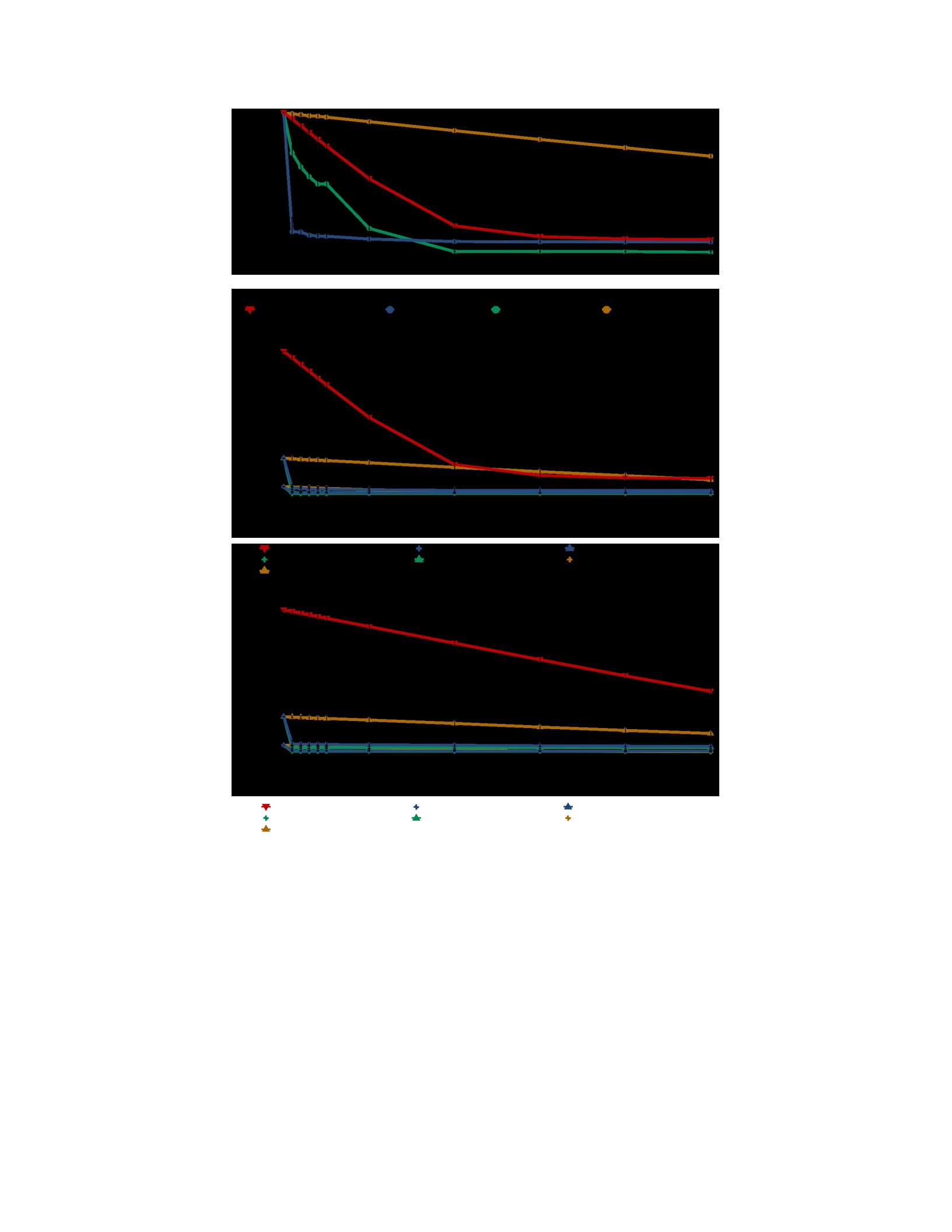
CHAPTER 5. NANOSATELLITE CONSTELLATION DESIGN 64
Bent pipeOEC (orbit- spaced, 5%)OEC (orbit-
spaced, 25%)
OEC (frame-spaced, 5%)OEC (frame-spaced, 25%)OEC (close-
spaced, 5%) OEC (close-spaced, 25%)
Figure 5.6: Top: Frame-spaced and orbit-spaced CNPs reduce downlink deficits without OEC by collecting data at
the GTFR. Close-spaced CNPs without OEC increase downlink deficits due to communication contention. Middle:
The same constellations enhanced with OEC; intelligent early discard leaves 5% to 25% of the data to downlink.
Bottom: Larger constellations experience worse performance under current practice, while OEC performance
remains consistent.
middle, but increases constellation population to 1000 nanosatellites. These data show that the bentpipe
architecture does not scale, suffering a high downlink deficit even with many ground stations. In contrast, CNP
configurations using OEC to discard data intelligently exhibit consistently low downlink deficits — even with an
increased constellation population. The bent-pipe architecture requires 3.5× more
Average System Latency per Ground Track Frame
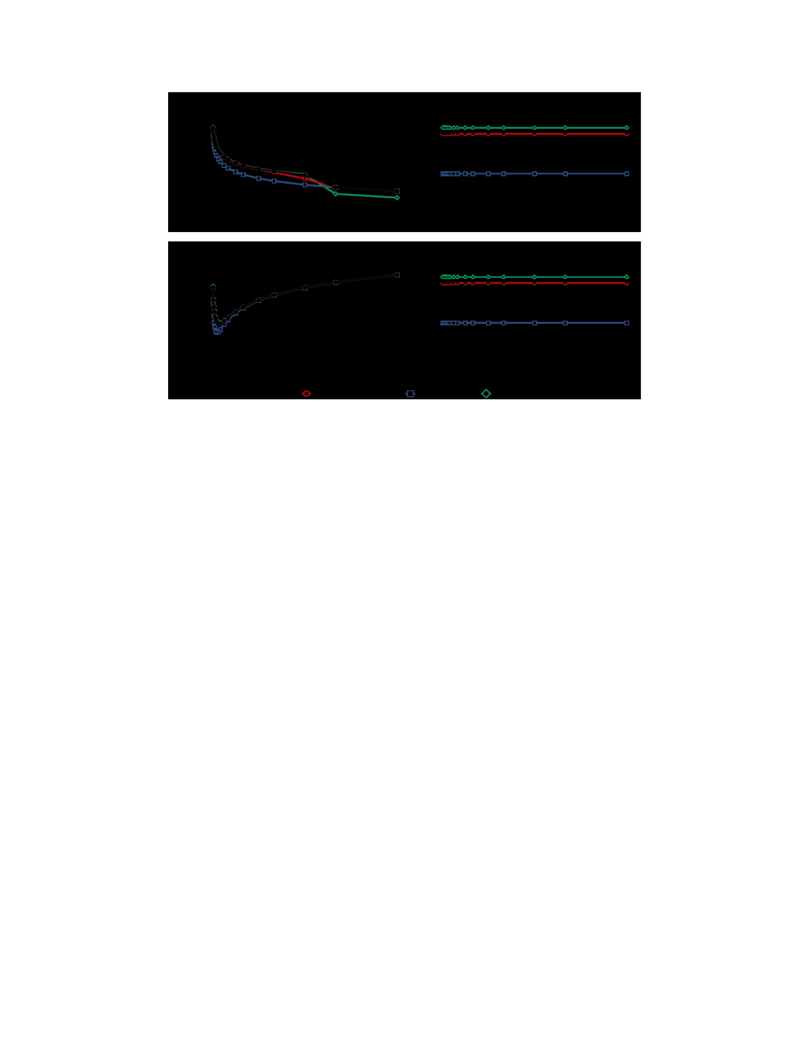
CHAPTER 5. NANOSATELLITE CONSTELLATION DESIGN 65
Figure 5.7: Left: Tile-parallel processing dramatically decreases system latency in close-spaced constellations.
Improvements disappear when satellites are frame-spaced. Right: System latency is high with frame-parallel
processing, but latency no longer depends on constellation configuration.
ground stations to service 1000 nanosatellites than to service 250 nanosatellites. OEC CNPs can use the same
ground infrastructure for constellations of both 250 and 1000 nanosatellites; OEC enables scaling up constellation
population without increasing ground infrastructure.
5.6.2 Pipeline Configuration Impacts Latency
This work uses cote-sim to simulate the CNP configurations described in Section 5.3.2 and evaluate OEC latency per
ground track frame, i.e. the time between frame capture and completion of frame analysis. This latency varies with
parallelization across a constellation and physical distance between nanosatellites in a CNP. System latency
determines the geographic location at which frame processing completes — an important factor when satellites
can transmit results only when in range of a ground station.
The system characteristics of frame-parallel CNPs are identical regardless of whether satellites are frame-
spaced or close-spaced. This fact is visible in Figure 5.7, right, by comparing the close-spaced, frame-parallel plot
with the frame-spaced, frame-parallel plot. In a frame-parallel CNP, the complexity of close-spaced formation flying
provides no benefit over an uncoordinated, frame-spaced configuration. Once each satellite has been assigned its
GTFs, relative drift between devices does not impact GTF latency.
However, the benefit of not requiring formation flying is tempered by uniformly high GTF latencies. Once
Coverage: Fraction of Ground Track Frames Captured
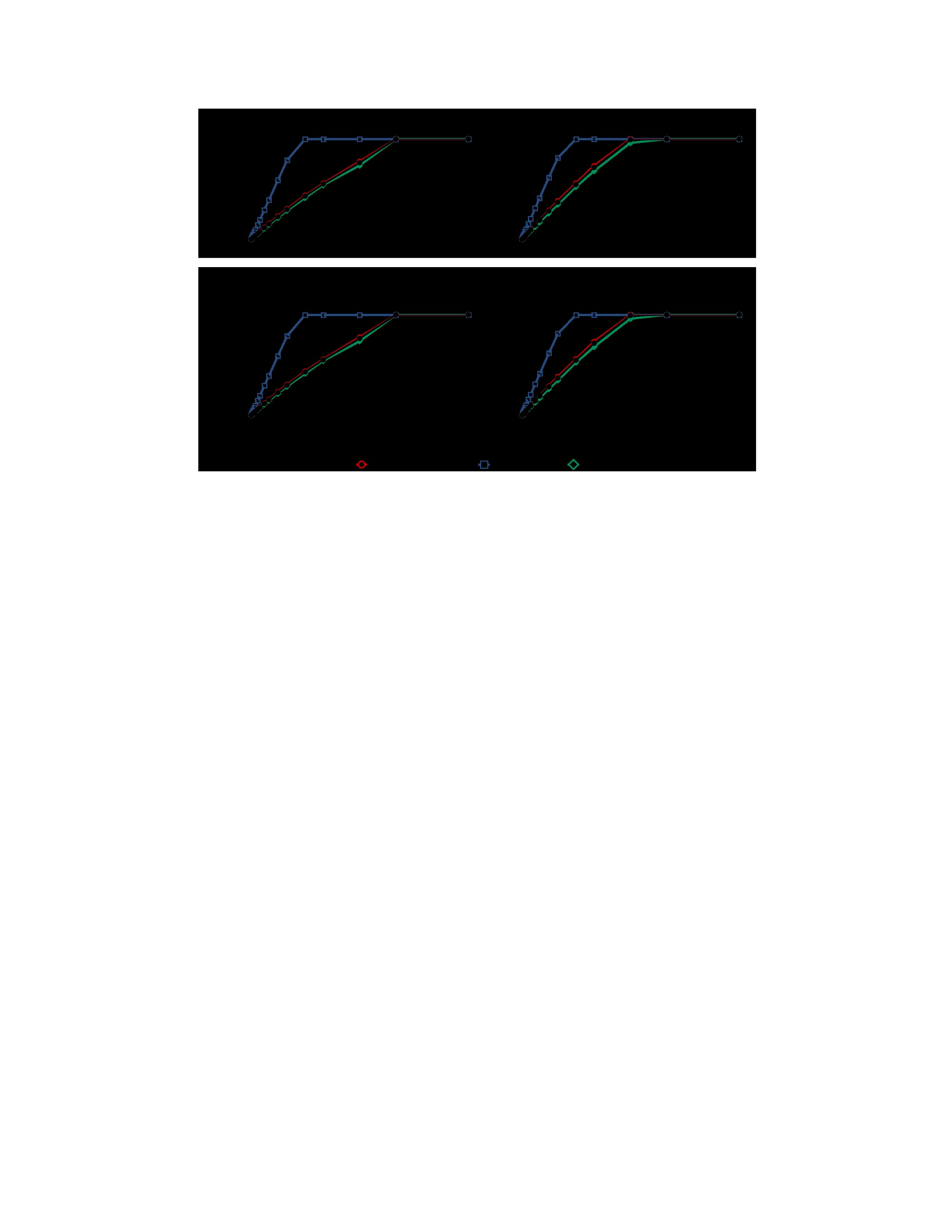
CHAPTER 5. NANOSATELLITE CONSTELLATION DESIGN 66
Figure 5.8: Coverage as a function of device count. Compared to the baseline, increasing overall system energy with
deployable solar panels strongly increases coverage.
the CNP pipeline is full, a new frame is completed every GTFP. Nevertheless, processing has long latency and the
geographic location at which a particular GTF completes processing is far from the original observation location.
Figure 5.7, left, shows that tile-parallel CNPs require a close-spaced configuration to maintain low per-GTF
latency. When devices are close-spaced, work is distributed among satellites and all tiles are processed shortly after
all satellites observe a frame. However, frame-spaced satellites have high per-GTF latency with deeper pipelines.
This effect emerges because, in a tile-parallel configuration, the satellite responsible for processing the last subset
of tiles captures the frame long after the first satellite captures the frame. This effect is magnified in an orbit-
spaced configuration. The data show that a close-spaced configuration reduces latency over 617×.
5.6.3 Collected Energy Impacts Coverage
This work uses cote-sim to simulate CNP configurations described in Section 5.3.2 and evaluate OEC ground track
coverage, i.e. the fraction of GTFs captured per revolution. To examine the impact of energy and computing on
coverage, this work varies energy buffer capacity, solar panel surface area, and computing hardware. This work
selects a baseline design with a 5.0 F capacitor bank, 7.1 W surface-mounted solar panels, and one Jetson TX2
compute module. It compares this baseline to a CNP of devices with
10.0 F capacitor banks (“more capacitance”), 14.2 W of power due to a deployable panel (“more power”), and two
Jetson TX2 modules (“more compute”).

CHAPTER 5. NANOSATELLITE CONSTELLATION DESIGN 67
Aggregate energy collected across a CNP limits coverage. As device count increases, a pipeline achieves the
minimum computing capability needed for full coverage before collecting sufficient aggregate energy to process all
frames. Figure 5.8 plots coverage as a function of pipeline depth. Each plot lists four series: the baseline
configuration, and the configurations with increased energy buffering, energy harvesting, and computing. Due to
the energy-constrained nature of this design point, increasing solar panel surface area increases coverage at a
faster rate than other parameters. While “more power” supports full coverage with a shorter pipeline, this
configuration depends on a complex, mechanically-deployed solar array that increases system cost and risks a
catastrophic deployer failure.
Under frame-parallel operation, individual satellites collect a GTF and process all tiles, which means that all
GTFs are imaged exactly once across the CNP system. As a result, the number of times that any camera is activated
across the CNP system matches the number of ground track frames as coverage approaches 100%. In tile-parallel
operation, every satellite images each GTF. Thus, the number of times that cameras are activated across the CNP
system is equal to the pipeline depth times the number of GTFs. However, the overall energy effect of more
frequent camera use at the system level is small because camera energy is four orders of magnitude less than
compute energy. The effect of more frequent camera activation manifests as a lower slope in the tile-parallel
graphs compared to the frame-parallel graphs as coverage approaches 100%. In Figure 5.8, the slopes in the tile-
parallel configurations are less steep than the slopes in the frame-parallel configurations.
The data show that for object detection, full coverage of the ground track is feasible under multiple
configurations, requiring around 100 satellites with deployable solar panels and around 250 satellites with surface-
mounted panels. Existing nanosatellite constellations contain more than 200 devices, which means that OEC
pipeline depths achieving full coverage are feasible. Increasing solar panel surface area dramatically reduces
pipeline depth at the expense of greater engineering complexity (deployable panels) and higher per-device cost.
Coverage degrades gracefully as pipeline depth decreases.
5.6.4 OEC Enables Online Autonomy
This work uses cote-lib to avoid the long reconfiguration time inherent to bent-pipe architectures. Uplink channels
are much lower in bitrate than downlink channels. Maximum downlink channel bitrate increases with receiver
gain; on Earth, receiver gain increases with dish diameter. Nanosatellites cannot increase receiver gain arbitrarily
due to physical restrictions on device size. Thus, uplinked data volume may
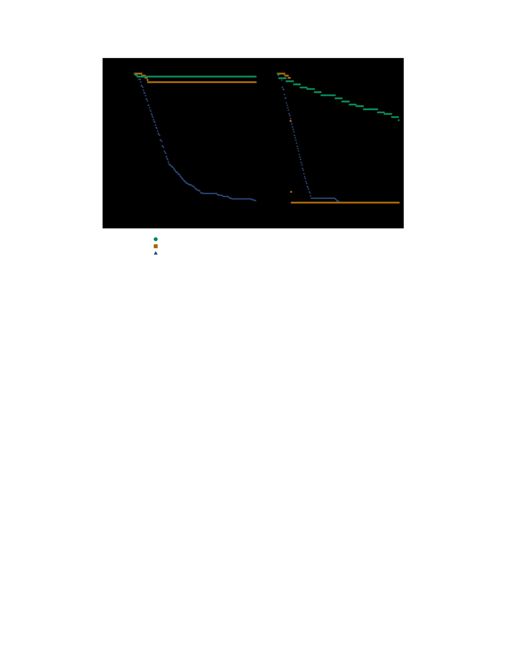
CHAPTER 5. NANOSATELLITE CONSTELLATION DESIGN 68
Close-spaced, equatorial constellation; equatorial ground
segment
Frame-spaced, inclined constellation; university ground
segment
Orbit-spaced, polar constellation; polar ground segment
Figure 5.9: Constellation configuration takes hours or more with bent pipes. Ground use of cote-lib enables shorter
configuration times for all constellation types, and use of cote-lib for OEC in space entirely eliminates configuration
delays.
be limited to kilobytes per pass. Larger constellations experience longer reconfiguration times because satellites
compete for uplink opportunities. Bent-pipe architectures require hours, days, or even months to reconfigure
existing constellations.
Satellites with onboard positioning (e.g. GPS) and knowledge of ground station locations are aware of
approaching link opportunities. However, under a bent-pipe architecture, remote-controlled satellites cannot
predict whether a ground station will establish a link session. Knowledge of upcoming communication events
allows satellites to intelligently choose between onboard processing and data transmission. cote-lib augments
ground segments by modeling satellite states; Figure 5.9 shows that cote-lib improves existing ground systems by
enabling link-schedule policies that prioritize communication to nanosatellites with the largest amount of data to
communicate, instead of heuristic policies that instead optimize for signal strength. The benefits of cote-lib are
greatest when used in space for OEC. Rather than a ground station forgoing valuable downlink opportunities to
upload link schedules, an OEC nanosatellite uses cote-lib to model the state of the entire constellation. With
knowledge of the link-
schedule policy, each nanosatellite generates upcoming communication events on orbit.
Figure 5.9 plots reconfiguration times with and without cote-lib. At left, ground stations operating under a bent-
pipe architecture use a highest-elevation link-schedule policy to maximize signal quality. At right, cote-lib augments

CHAPTER 5. NANOSATELLITE CONSTELLATION DESIGN 69
existing ground segments by enabling a more advanced link-schedule policy prioritizing satellites with the largest
amount of buffered data. Ground use of cote-lib reduces reconfiguration times, but constellations of tens to
hundreds of devices often require multiple revolutions before the entire system reconfigures. During this time, the
constellation misses thousands of GTFs. cote-lib avoids lengthy reconfiguration times. By running continuously in
the background on an OEC satellite, computing and communication decisions can be made autonomously on orbit.
5.7 Related Work
Several categories of work relate to orbital edge computing. Section 5.1 provides a brief space systems background.
The NASA guide to the state-of-the-art in small satellites [265] describes characteristic aspects of nanosatellites,
including technology readiness levels of essential subsystems. Recent surveys [15, 151] study multi-satellite orbital
dynamics and provide an overview of propulsion systems. Commercial efforts demonstrate the viability of camera-
equipped nanosatellite constellations [61, 180]. The SpaceNet challenge [246] illustrates broad interest in visual
computing on space data, and the proposed Amazon ground station network [5] further cements the value of
computing on visual and other space sensor data.
Recent edge computing work provides context for this work. Edge computing recognizes that, as high-datarate
sensors (e.g. cameras, lidar) proliferate, streaming all data to central cloud systems for processing becomes
infeasible [199, 198, 255]. Edge computing is important particularly in cases of complex processing, e.g. video
querying [100], search [133], or DNN speech processing [124]. This work proposes to leverage early discard, which
has been studied for search [101], video indexing [100], and drone video processing [255]. Recent work [202, 24]
demonstrates the utility of simulation frameworks for edge computing on drones; cote is an analogous utility for
the orbital edge. Machine inference accelerators [65, 31, 87, 36] could significantly shorten full-coverage CNP
pipeline depths, although some that rely on temporal data redundancy [26] may have limited benefit for devices
capturing images at the GTFR.
Intermittent computing [149] shares challenges with orbital edge computing in that both types of systems are
fully energy-autonomous. A number of recent intermittent systems [155, 95, 154, 44, 153, 121] function despite
unpredictable power failures using techniques that may be applicable to the orbital edge in future work. Some
intermittent computing platforms [46] are similar in that they rely only on supercapacitors for energy storage.
Other intermittent systems are similar in that they target DNN workloads [83] and communication minimization
[152] at the edge in batteryless devices. While similar in spirit, these efforts differ significantly in scale, deployment
environment, and in their inability to rely on processor sleep modes; instead, they power off frequently.

CHAPTER 5. NANOSATELLITE CONSTELLATION DESIGN 70
5.8 Summary
This work develops orbital edge computing: edge computing on orbit using processing resources colocated with
sensors inside small, low-cost satellites. The low cost of a nanosatellite compared to monolithic satellite systems
makes large satellite constellations feasible for the first time. Applications of this emerging technology are impeded
by existing, bent-pipe architectures. Orbital edge computing provides responsiveness, reliability, and scalability
benefits. Future work should study energy collection and storage for orbital edge computing and radiation-
hardened, machine-learning (ML) accelerators.
For example, this work observes that incomplete ground track coverage stems from the energyconstrained,
intermittent nature of these nanosatellites. Once a constellation, in aggregate, collects sufficient energy for full
coverage, high processing latency can still limit coverage. Increasing energy availability with deployable solar panels
is unsatisfactory, because this solution raises mission cost and mission risk. As an alternative solution, future work
could investigate energy-efficient, domain-specific accelerators (DSAs) for orbital edge computing workloads.
Future work could evaluate the architectural vulnerability factors (AVFs) of recently-proposed ML accelerators and
propose new ML accelerators that operate intermittently in the space environment.
While this work has focused on nanosatellite constellations that share a single orbit and a single workload,
future work may investigate heterogeneous systems and heterogeneous workloads. For example, a constellation
operator may wish to serve many different clients over time. Clients will be interested in different features at
different scales. As a result, different orbit altitudes and different hardware will be better suited to different clients.
Supporting a dynamic set of workloads from a dynamic set of clients poses an interesting challenge, especially with
regards to constellation reconfiguration. The high overhead of uplinking new ML models could be offset with
federated learning techniques.
Looking forward, deployments of satellites that are even smaller than nanosatellites are expected. Chip-scale or
gram-scale satellites (“chipsats”) can be deployed more numerously and at even lower cost. Such devices are even
more attritable than nanosatellites, but the smaller size places even tighter constraints on capability. Successful
operation of these emerging devices will require the application of orbital edge computing techniques.

Chapter 6
Scheduling Satellite Operations
As emerging launch platforms provide increased access to low-Earth orbit (LEO), satellite systems proliferate [64,
78]. Several organizations have filed plans to deploy an unprecedented amount of satellites to LEO [196, 197, 96,
97, 98, 226, 228, 227]. The standardization of the “cubesat” form factor [167] stimulated rapid growth in
nanosatellite deployments across the last two decades [224]. Recent work identifies emerging challenges
stemming from these trends [52, 53, 148]; a more crowed LEO requires new approaches to satellite management.
As LEO proliferates with new satellite constellations, existing approaches to space vehicle (SV) operations break.
Large, expensive SVs of the past rely on a communication model that sends remote control commands to orbit and
delivers raw, unprocessed data to Earth; this design is referred to as a “bent pipe” by space system architects [136].
Emerging nanosatellite constellations continue to utilize this approach for space system operations [61]. However,
as constellation population increases, this approach grows increasingly infeasible [52, 53].
Recent work proposes distributed ground stations [247] and orbital edge computing (OEC) [52, 53] to alleviate
the challenges of the bent pipe. This work quantifies the limitations of recent proposals utilizing edge computing in
space. It examines the static scheduling used by recent proposals, and it proposes a dynamic system that adapts to
satellite conditions as they occur on orbit. This work presents Horizon: a system for dynamically scheduling satellite
operations in order to improve support for edge computing in space.
This chapter presents the following contributions: (i) it identifies challenges in satellite operations under the
existing proposals of bent-pipe and static computational nanosatellite pipelines (CNPs); (ii) it identifies four key
measures of satellite performance: energy, data, computation, and communication; (iii) it presents Horizon — a
system to support dynamic scheduling of satellite jobs in space — which
75
consists of three components: offline operator characterizations, client job requests, and a reactive, online
scheduler; and (iv) it shows that Horizon supports a more than 81% increase in processed data downlinked per
orbit period and, for energy-constrained systems, a more than 36% increase in unprocessed data downlinked per
orbit period.
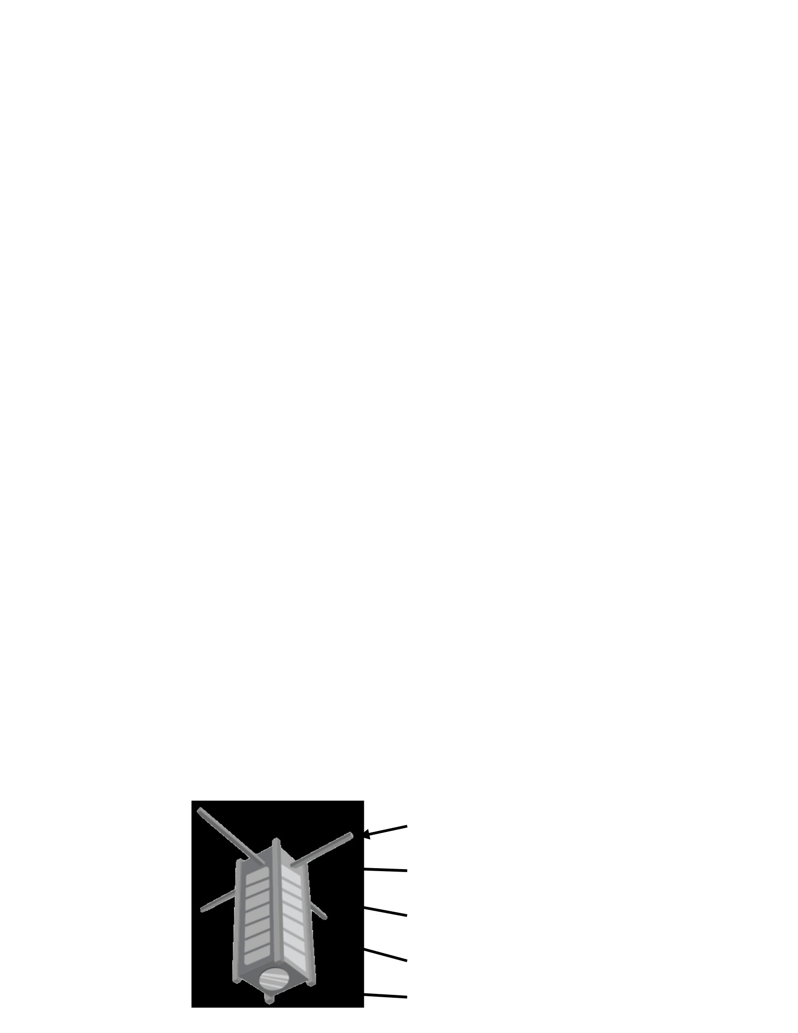
CHAPTER 6. SCHEDULING SATELLITE OPERATIONS 72
6.1 Earth-observation Satellite Systems
Historically, Earth-observation satellites have been operated as large, monolithic systems with a narrowlyscoped
purpose. Individual satellites cost hundreds of millions of US dollars, encouraging a focus on reducing risk at the
expense of capability. For example, the $192,000,000, 500 kg Earth Observing-1 (EO-1) is a “one-of-a-kind” [168]
satellite with a 16 year mission that ended in 2017. EO-1 contains a 12 MHz Mongoose-V CPU, which implements
the 32-bit MIPS ISA, to demonstrate autonomous science [38]. The limited capability of this onboard computer
supports risk-mitigation; chip area dedicated to redundancy and other radiation-hardening techniques prevents
incorporation of other, state-of-the-art features.
However, historical analysis of such missions suggests that these risk-mitigation techniques may be over-
engineered. The 16-year EO-1 mission began with a predicted lifespan of just one year [168]. Excessive margin
appears in other aspects of Earth-observation satellite operation. For example, solar panels harvest more energy
than the satellite can store, satellites carry more fuel than can be used during the mission lifespan, and satellites
observe more data than can be downlinked per revolution. These inefficiencies arise from a function-focused
approach to satellite operation: space system engineers design and operate satellites for a narrowly-scoped
function — naturally including excessive margin to ensure success.
More recently, Earth-observation satellites have shifted toward collections of numerous nanosatellites. The
small size of a nanosatellite, which is dictated by the cubesat standard [167], allows for launch of many devices at a
relatively low per-satellite cost. Standardization creates a market for commercial, offthe-shelf (COTS) subsystems,
which lowers costs. Reduced cost lowers risk and opens opportunities to decrease margins, e.g. by deploying state-
of-the-art computers that are merely radiation-tolerant rather than radiation-hardened.
Nevertheless, recent systems still operate under a function-focused design. For example, Planet Labs originally
aimed to deploy a constellation that images the entire Earth daily [63]. After finding the operation of such a system
to be infeasible, the company instead deployed a constellation that images the entire landmass of Earth daily. This
function-focused goal is achieved with a new kind of margin: constellation population and ground station count.
Planet Labs deployed satellites and ground stations until achieving the mission.
Anatomy of a Nanosatellite
Communications
CHAPTER 6. SCHEDULING SATELLITE OPERATIONS 73
Attitude Determination and Control (ADACS)
Command and Data Handling (C&DH)
Energy Harvesting
Sensors
Key Performance Factors
EnergyComputation
DataCommunication
Figure 6.1: Nanosatellites have a mass between 1 and 10 kg and are centimeters in size. Typically, satellites act as
dumb, remote-controlled sensors with little processing at the edge. Horizon enables intelligent scheduling of
onboard processing.
For satellite systems, this function-focused approach to operations makes efficiency difficult. A focus on
function obscures the limiting constraints, resulting in over-engineering and excessive margins — often
unintentionally or even invisibly. In order to support efficient operation of future satellite constellations, this work
proposes an alternative to the historical practice of function-focused operation.
6.1.1 Constraints-Focused Satellite Operations
This work proposes a fundamental shift in the operation of satellite systems. Instead of a functionfocused approach
to satellite design and operation, this work proposes a constraints-focused approach. It identifies four fundamental
constraints of Earth-observation satellite systems, and it concludes that management of these constraints
determine the operational efficiency. See Figure 6.1 for an overview of a typical nanosatellite and the performance
factors affecting its utility.
Energy: Unlike terrestrial computer systems and sensors, satellites cannot obtain energy from a wired electrical
grid. All energy obtained by a satellite must be harvested from its environment. Satellites typically harvest solar
energy with an array of solar cells. Satellites place harvested energy into an energystorage device, such as a battery

CHAPTER 6. SCHEDULING SATELLITE OPERATIONS 74
or a capacitor, for later consumption by subsystems. This work identifies two energy constraints affecting satellite
operation: insufficient power and energy buffer overflow. In the case of insufficient power, the harvested and
stored energy cannot power the active satellite subsystems. In the case of an energy buffer overflow, the energy-
storage device cannot accept surplus harvested energy.
Data: A typical Earth-observation satellite completes a full revolution around the Earth in roughly 90 minutes.
As a result, each satellite has the opportunity to capture a large quantity of data during each revolution. Captured
data is placed into a data-storage device. This work identifies two data constraints affecting satellite operation:
insufficient data rate and data buffer overflow. In the case of insufficient data rate, the satellite has been tasked
with collecting too few of the scenes it observes, resulting in idleness. In the case of a data buffer overflow, the
data storage device cannot accept additional observations.
Computation: The purpose of an Earth-observation satellite is to produce useful observations. However,
depending on the operation of the satellite, very little of its potential observations may be useful. Computation
accepts raw data (sensor output) as input in order to distinguish between high-value data (the desirable portion of
raw data) and low-value data (raw data that is not high-value data). The resulting high-value data may have been
transformed by the computation; for example, a binary classifier may accept a raw image as input and output a
“zero” or a “one” to indicate the absence or presence of a feature of interest. The effective compression ratio of a
computation is the ratio between the input data quantity and the output data quantity. The execution time of a
computation is the duration of the computation. Existing satellite systems operating under a bent-pipe architecture
perform little or no computation on orbit. This work identifies three factors which together determine the utility of
a computation: energy cost, time cost, and the effective compression ratio.
Communication: Ultimately, observations captured by an Earth-observation satellite must be transmitted to the
ground segment. These results are relayed via a radio (or, in some cases, an optical) link. Often, communication
opportunities are limited because ground stations are rarely in view. When available, a communication link may
transmit raw data or transformed data at a given bit rate. Operating the communication link often requires a
significant amount of power. This work identifies two factors that determine the utility of a communication: energy
cost and time cost.
Regardless of the system characteristics or application, any inefficiency in these factors reduces device
performance. Using typical function-focused design and operation, avoiding such inefficiencies is difficult. This work
proposes a scheduler that manages device operation to make efficient use of these factors
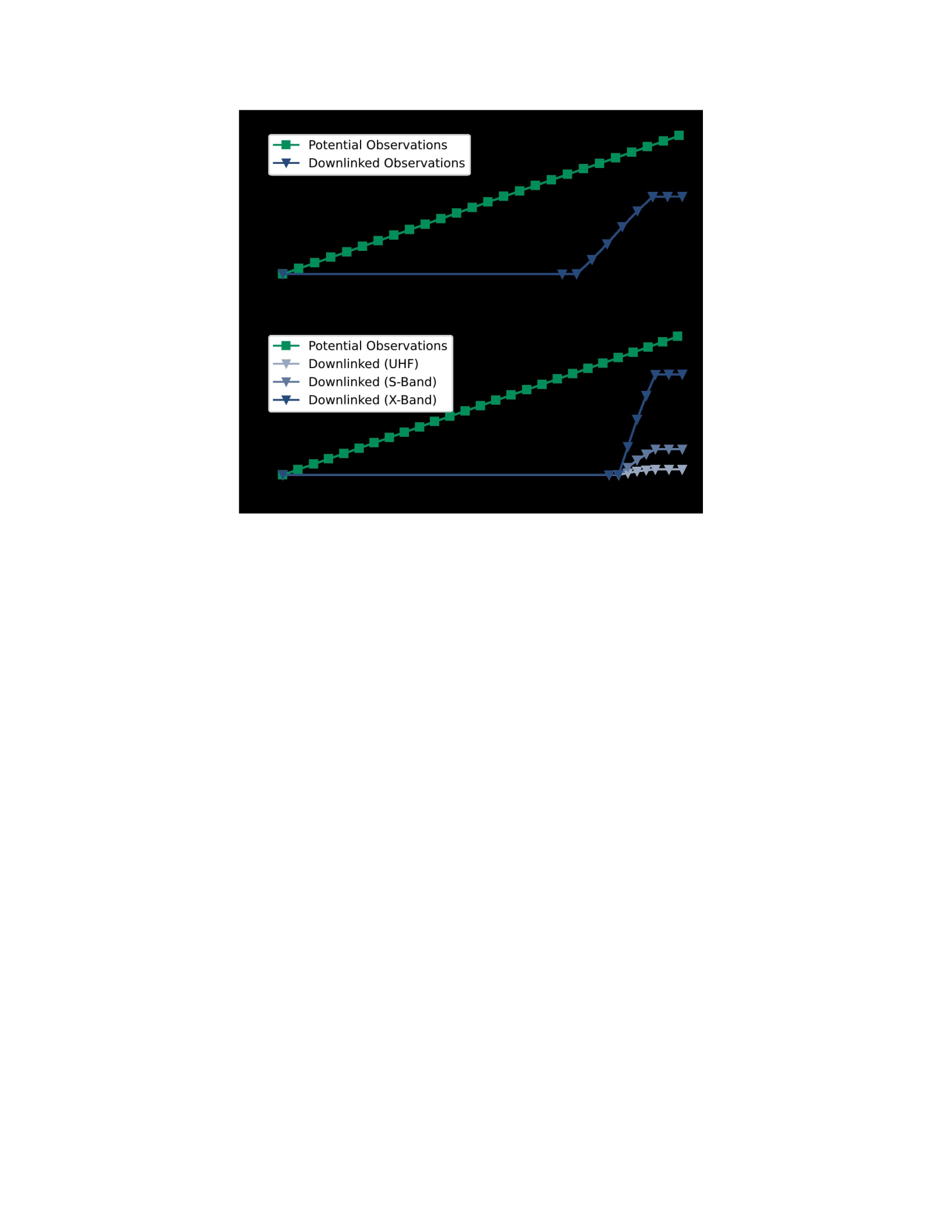
CHAPTER 6. SCHEDULING SATELLITE OPERATIONS 75
Figure 6.2: Top: The downlink bottleneck quantified for a large, monolithic satellite. During just half its orbit
revolution, the satellite has the opportunity to observe more ground track frames than can be downlinked. Bottom:
The downlink bottleneck quantified for a modestly-sized nanosatellite constellation of 20 devices. Contention for
downlink time prevents potential observations from transmission.
through a constraints-focused approach.
Earth-observation satellite systems are uniquely positioned to enable useful prediction and measurement of
these constraint factors. In low-Earth orbit, the available solar energy is well-known and predictable. Predicted
energy availability can be improved with in-situ, real-time measurements. Welldefined astrodynamic equations
make data collection predictable. Computation can be characterized before deployment to satellite hardware. The
large distances and vacuum of space make satellite communication uniquely predictable.
This work proposes Horizon, the first onboard scheduler for satellite systems that combines physics simulations,
real-time measurements, and client requests to optimize energy, data, computation, and communication to
improve device utility.
6.2 Motivation
Horizon accepts client job requests and, given knowledge of satellite characteristics by the constellation operator,
schedules tasks to maximize system utility. Thus, Horizon must be aware of constraints limiting task performance.
This section presents charts motivating constraints relevant to a satellite task scheduler. It highlights how these
constraints interact and show how examining each only in isolation creates unrealistic performance expectations.

CHAPTER 6. SCHEDULING SATELLITE OPERATIONS 76
System characteristics determine which resource depletes first (i.e., which resource acts as the primary constraint
or bottleneck on system performance).
The following experiments model the real, polar orbits of Earth-observation satellites. This work locates ground
stations at their actual, real-world positions near the poles (which maximizes communication opportunity; see
Figure 2.2). When a polar-orbit satellite cannot downlink all data during half of an orbit revolution, it continues to
“fall behind” during subsequent interludes due to the periodic nature of orbital mechanics. Active research efforts
[247, 249, 209, 210] consider ground stations placed at other, less-frequently used locations; balancing the cost and
utility of such a ground segment remains an open question.
6.2.1 The Downlink Bottleneck
Figure 6.2, top, quantifies the downlink bottleneck for a large, monolithic satellite. This work models Sentinel-2A
operated by the European Space Agency (ESA) with a mass of about 1200 kg and dimensions of about 3.4 m×1.8
m×2.4 m [260]. This Earth-observation satellite captures images across 13 spectral bands with a swath of 290 km.
Visual-spectrum bands achieve a GSD of 10 m/px, and other bands achieve GSDs of 20 m/px and 60 m/px. Using
the cote simulator [53], altitude averages about 798 km during half of an orbit revolution (about 50 min, 19 s in
duration). According to the Sentinel High Level Operations Plan (HLOP) [181], data production averages 160 Mbit/s
after compression. Using cote, this work finds that Sentinel-2A has the opportunity to capture about 60 GB of
compressed frames during half of an orbit
revolution.
Sentinel-2A downlinks data with two X-Band radios, each achieving a peak of 260 Mbit/s, to Svalbard in Norway
[181]. Using cote, this work finds a downlink duration of about 10 min, 21 s with a peak, combined downlink rate of
523 Mbit/s and a minimum rate of 414 Mbit/s. Thus, Sentinel-2A downlinks only about 37 GB during half of an
orbit revolution. The downlink bottleneck arises from the fact that Sentinel-2A transmits only 37 GB of a potential
60 GB of observations. In practice, satellite operators manually task the device to collect a subset of potential
observations. With OEC, the satellite captures all frames and intelligently discards low-value observations.
Figure 6.2, bottom, quantifies the downlink bottleneck for a constellation of 3U cubesats. This work models a
UHF radio [189, 190] and ground station [129], an S-Band radio [117, 116] and ground station [115], and an X-Band
radio [215, 214] and ground station [135] using cote. The COTS ground station resides in Washington State, and the
20 nanosatellites space equidistantly in the Flock 4Y-10 [32] 3U cubesat orbit. Each device captures three-channel,
4208 × 3120 px images with a GSD averaging about 2.9 m/px. Altitude averages about 523 km during half of an
orbit revolution (about 47 min, 26 s in duration). Data production averages about 15 Mbit/s after compression;
each device has the opportunity to capture about 5.4 GB of compressed frames during half of an orbit revolution.

CHAPTER 6. SCHEDULING SATELLITE OPERATIONS 77
With a COTS UHF radio, maximum-achievable bitrates range from 3.1 Mbit/s to 9.0 Mbit/s. With a COTS S-Band
radio, maximum-achievable bitrates range from 22 Mbit/s to 36 Mbit/s. With a COTS X-Band radio, maximum-
achievable bitrates range from 94 Mbit/s to 130 Mbit/s. These are maximumachievable bitrates under known
physics reported by cote simulation of the COTS radio systems as described by their datasheets; in practice, usable
datarates are likely to be much lower due to encoding redundancies, protocol overheads, environmental
attenuation, and imperfect alignment of antenna gains. During half of an orbit revolution, the UHF radio downlinks
about 0.23 GB, the S-Band radio downlinks about 1.1 GB, and the X-Band radio downlinks about 4.2 GB.
For a nanosatellite constellation, the downlink bottleneck arises from an imbalance between communication
opportunities and data production rate (as in the monolithic case), as well as from contention for ground station
time. One nanosatellite could downlink to a ground station for about 7 min, 29 s per pass (given sufficient energy;
see Section 6.2.3). However, for a modest constellation of 20 devices, the ground station observes many satellites
simultaneously. To serve every device, the station receives data from a particular nanosatellite for only about 4
min, 41 s per pass; a high-gain antenna must choose a satellite at which to point its narrow receiving beam.
Contention worsens as nanosatellite count grows; existing and emerging constellations consist of 100s or 1000s of
devices.
6.2.2 The Computational Bottleneck
To quantify the computational bottleneck for edge computing systems in space, this work considers the near-
universal nuisance of clouds in Earth-observation images. Analysis of NASA data indicates that clouds obscure
about two-thirds of pixels on average [127]. Thus, discarding cloud pixels before downlink could produce a filtered
data quantity averaging one-third that of raw data. After identifying regions clear of clouds, clients may wish to
deploy additional filters to identify vegetation, weather events, or buildings and other infrastructure.
This work assesses the computational bottleneck for a monolithic satellite supporting OEC and a computational
nanosatellite. Scenario characteristics remain unchanged from Section 6.2.1. For cloud filtering, this work models
the fastest, pixel-segmentation, neural network from other OEC work [51]. It performs naive frame tiling: each
frame splits into non-overlapping tiles equal to neural network input
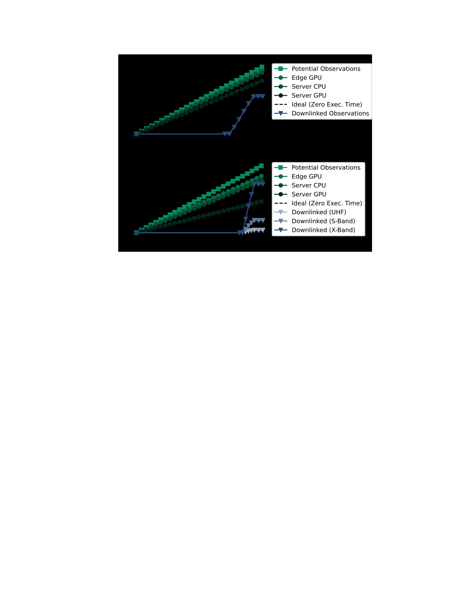
CHAPTER 6. SCHEDULING SATELLITE OPERATIONS 78
Figure 6.3: Top: The computational bottleneck quantified for a monolithic satellite supporting OEC. After filtering
clouds with a server GPU, data quantity still exceeds downlink capacity because execution time per frame exceeds
frame rate. Bottom: Ignoring SWaP-C limits, only a server GPU filters enough frames to alleviate the downlink
bottleneck despite execution time still exceeding observation rate.
size. Other OEC work [52, 51] finds that naive tiling can produce poor accuracy; smaller, more numerous tiles can
improve accuracy at the cost of greater execution time per frame (see Section 6.1, data quality
constraints).
Importantly, Figure 6.3 does not consider energy or power constraints; see Section 6.2.3 for an evaluation of
the energy bottleneck. This characterization quantifies improvements when (i) sufficient energy exists to support
the computations, and (ii) the application filters the data with perfect accuracy.
Figure 6.3, top, illustrates data quantity reduction on a monolithic satellite supporting OEC. The satellite
observes a new frame about every 43 s on average. An edge GPU filters a frame in about 490 s, a server CPU filters
a frame in about 350 s, and a server GPU filters a frame in about 140 s. Thus, less than 9%, 13%, and 31% of
observations are filtered, respectively, and remaining observations queue for downlink at the full, raw data
quantity. None of the computer hardware executes the application fast enough to reduce data quantity below the
downlink capacity. However, as shown by the dashed line, further reducing execution time eventually produces an
OEC operating point addressing the downlink bottleneck.
Figure 6.3, bottom, illustrates data quantity reduction on a computational nanosatellite. The satellite observes a
new frame about every 1.7 s on average. An edge GPU filters a frame in about 7.4 s, a server
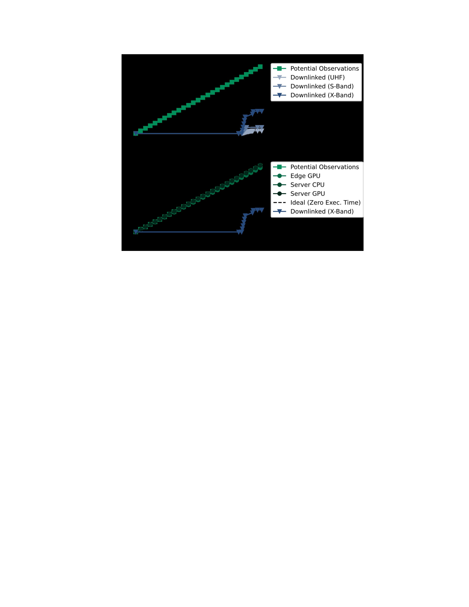
CHAPTER 6. SCHEDULING SATELLITE OPERATIONS 79
Figure 6.4: Top: When accounting for nanosatellite energy constraints, the downlink bottleneck worsens. Radios
drawing high power cannot operate continuously throughout a communication opportunity. Bottom: Energy
constraints exacerbate the computational bottleneck. The slowest but most energy-efficient platform filters the
most data.
CPU filters a frame in about 5.3 s, and a server GPU filters a frame in about 2.1 s. Thus, less than 23%, 32%, and
80% of observations are filtered, respectively, and remaining observations queue for downlink at the full, raw data
quantity. Only the server GPU potentially reduces data quantity below the X-Band downlink capacity. However, as
shown in Section 6.2.3, energy limits prevent the server GPU from actually achieving this operating point. Size
constraints also prevent deployment of a server GPU inside a 3U cubesat.
6.2.3 The Energy Bottleneck
To quantify the satellite energy bottleneck, this work focuses on COTS nanosatellites. Sentinel-2A harvests about
1700 W at its projected end-of-life (EOL), and power consumption averages 1400 W [260]. A server GPU drawing
about 180 W, although not rated to survive the space environment, conceivably could operate continuously in
terms of power. In contrast, a 3U cubesat with surface-mounted solar cells [212] harvests less than 7.1 W at its
EOL. During operation, radio and computer subsystems often draw more power than such a solar array harvests,
making the device energy-constrained: average, operational energy consumption exceeds average energy
harvested.
Figure 6.4, top, shows that energy constraints affect the data downlinked from a nanosatellite without
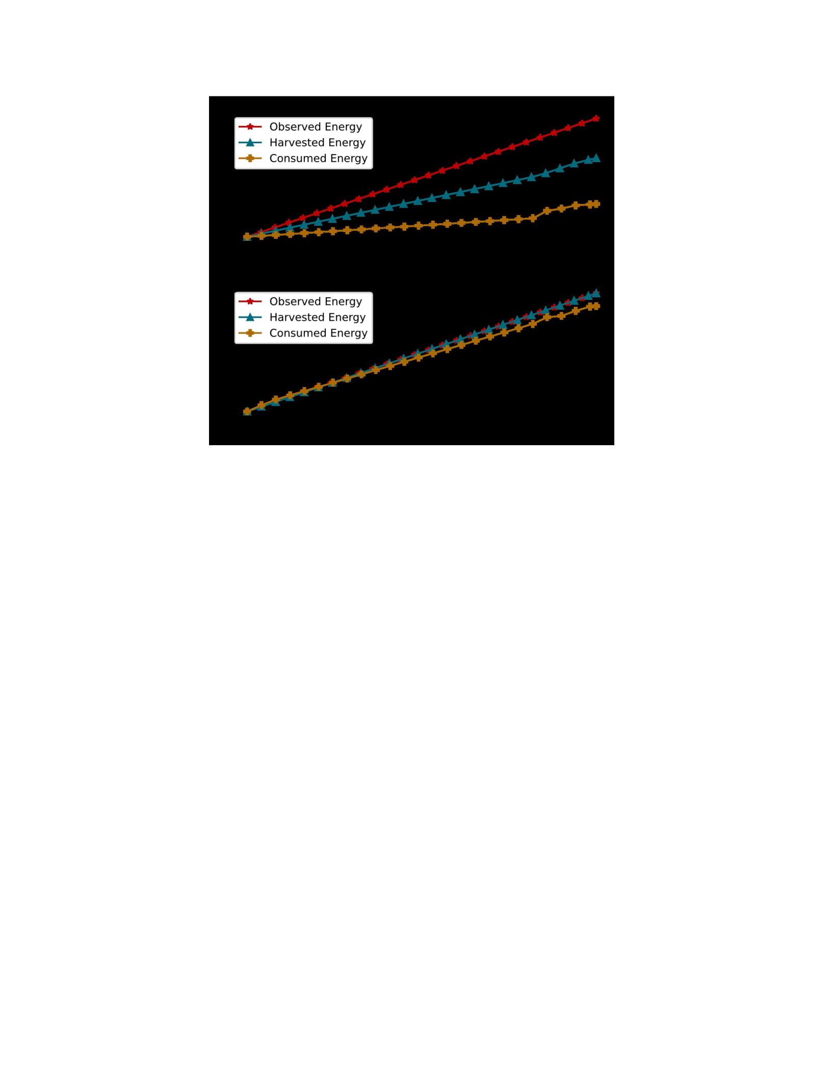
CHAPTER 6. SCHEDULING SATELLITE OPERATIONS 80
Figure 6.5: Top: Without edge computing on orbit, much of the energy observed cannot be harvested because the
energy buffer is full. Bottom: An energy-constrained, computational nanosatellite harvests and consumes all
observed energy. Horizon increases satellite utility by scheduling efficient energy consumption among subsystems.
OEC (compare to Figure 6.2, bottom). Accounting for power, the UHF radio still downlinks about 0.23 GB because it
does not experience an energy constraint. However, the S-Band radio downlinks about 0.53 GB (48% of the case
without energy constraints), and the X-Band radio downlinks about 1.9 GB (45% of the case without energy
constraints). Neither the S-Band radio nor the X-Band radio operate continuously during the communication
session; both must pause to refill the energy buffer.
Figure 6.4, bottom, shows that energy constraints affect computational nanosatellites as well (compare to
Figure 6.3, bottom). The edge GPU filters less than 7% of observations (instead of 9%); the server CPU filters less
than 1% of observations (instead of 13%); and the server GPU filters less than 2% of observations (instead of 31%).
When the satellite is energy-constrained, the slower, more energy-efficient edge GPU filters more data than faster,
less energy-efficient alternatives.
Energy buffer overflow: A large corpus of energy-constrained, embedded system research in intermittent
computing assumes the on-device energy buffer fully recharges before resuming operations after buffer depletion
[194, 147, 43, 154, 45, 46, 193, 155, 174, 159, 221, 60]. One such work dynamically resizes the physical buffer
capacity to meet varying reactivity and atomicity requirements [46]. Horizon makes a different observation. While
the energy buffer of an energy-harvesting device is full, no additional, harvested energy can be stored. For an

CHAPTER 6. SCHEDULING SATELLITE OPERATIONS 81
energy-constrained device (i.e., one with utility limited by a lack of energy), this opportunity cost reduces
performance. This work refers to this situation as an energy buffer
overflow.
Figure 6.5 quantifies the impact of an energy buffer overflow in nanosatellites. Here, this work models a
relatively large (in both physical volume and energy capacity) energy buffer of three supercapacitors in series [211].
Figure 6.5, top, shows that a nanosatellite without OEC harvests much less energy than it observes. Such a satellite
operates at an energy deficit only during relatively infrequent communication sessions; most of the time, no
ground station is in range and, once the energy buffer fills, surplus observed energy cannot be harvested.
Figure 6.5, bottom, shows that an energy-constrained, computational nanosatellite harvests and consumes all
observed energy. The onboard computer regularly depletes the energy buffer so that all observed energy can be
harvested. However, simply harvesting and consuming all observed energy is not enough. For example, an onboard
computer that filters more data than the radio downlinks wastes energy; satellite utility would increase if the
wasted energy had been used to improve radio uptime. Horizon increases satellite utility by scheduling efficient
energy consumption among device subsystems.
6.3 Existing Limitations and Shortcomings
Ground segments operate existing satellites as dumb, remote-controlled sensors. Space system architects refer to
this approach as a bent pipe: satellites respond to commands from the ground by downlinking raw, unprocessed
sensor data [136]. Emerging nanosatellites, which leverage large device counts, continue to adhere to the bent-
pipe approach to operations. This design results in a downlink bottleneck: the rate of new satellite observations
outpaces the rate of data downlink [53].
To address this downlink bottleneck, recent work proposes static computational nanosatellite pipelines (static
CNPs): satellites processing captured data at the orbital edge in order to select intelligently highvalue data for
downlink and to discard low-value data at the edge [53]. This approach addresses energy and computation
constraints using high device counts to distribute tasks across satellites. However, this approach is function-focused
and makes use of a new kind of engineering margin for space systems: constellation population. With a constraints-
focused approach to operations, the improvements offered by orbital edge computing are extended.
6.3.1 Bent-Pipe Scheduling
In order to understand the limitations and shortcomings of existing satellite operations, this work examines a bent-
pipe scheduling system. A typical, Earth-observation satellite operating under a bent-pipe architecture includes an
attitude determination and control system (ADACS), a sensor such as a camera, and a communication system to

CHAPTER 6. SCHEDULING SATELLITE OPERATIONS 82
transmit and receive data. Any onboard computers are low-power, relatively low-performance systems for
command and data handling (C&DH).
This work uses the open source satellite simulation software cote to design and evaluate the operation of such
a system [53]. The bent-pipe, Earth-observation nanosatellite orbits the Earth in a typical polar orbit with an
altitude ranging between 487 km and 500 km. When power is available, the ADACS points the camera system to
the nadir, i.e. directly toward the Earth for image capture [2]. The camera system is comparable to state-of-the-art,
Earth-observation nanosatellite platforms, providing a ground sample distance (GSD) ranging between 2.68 m/px
and 2.75 m/px [213]. This work models the communication systems using datasheets from commercial, off-the-
shelf (COTS) nanosatellite components [109, 84, 108, 113, 114].
A reactive, bent-pipe approach to satellite operations uses signals to trigger satellite actions. New ground track
frames (GTFs) are captured based on position information provided by the onboard GPS (global positioning system)
receiver. Communication sessions are initiated and managed by the ground segment when the satellite is in range
of a ground station. Under this baseline, the satellite is able to downlink only ten percent of high-value data during
one revolution with nearly 68% of raw data remaining on orbit.
6.3.2 Static CNP Improvements
Recent work proposes intelligent early discard of low-value data before transmission to a ground station [52]. To
perform intelligent early discard, the satellite must support orbital edge computing. Emerging nanosatellites can
include state-of-the-art, embedded processors that are merely radiation tolerant because the risk per device is low.
The nanosatellite will have been replaced before radiation inhibits device operation.
This work again leverages cote to design and evaluate the operation of such a system. For intelligent early
discard, this work modifies the previous scenario by adding onboard computing. When power is available, an
embedded processor performs machine-learning image analysis at a rate of 22.3 frames per second. This work
models the processing module using measured execution time and power of COTS components [177].
Figure 6.6 illustrates how static CNPs improve the fraction of high-value data downlinked per rev-
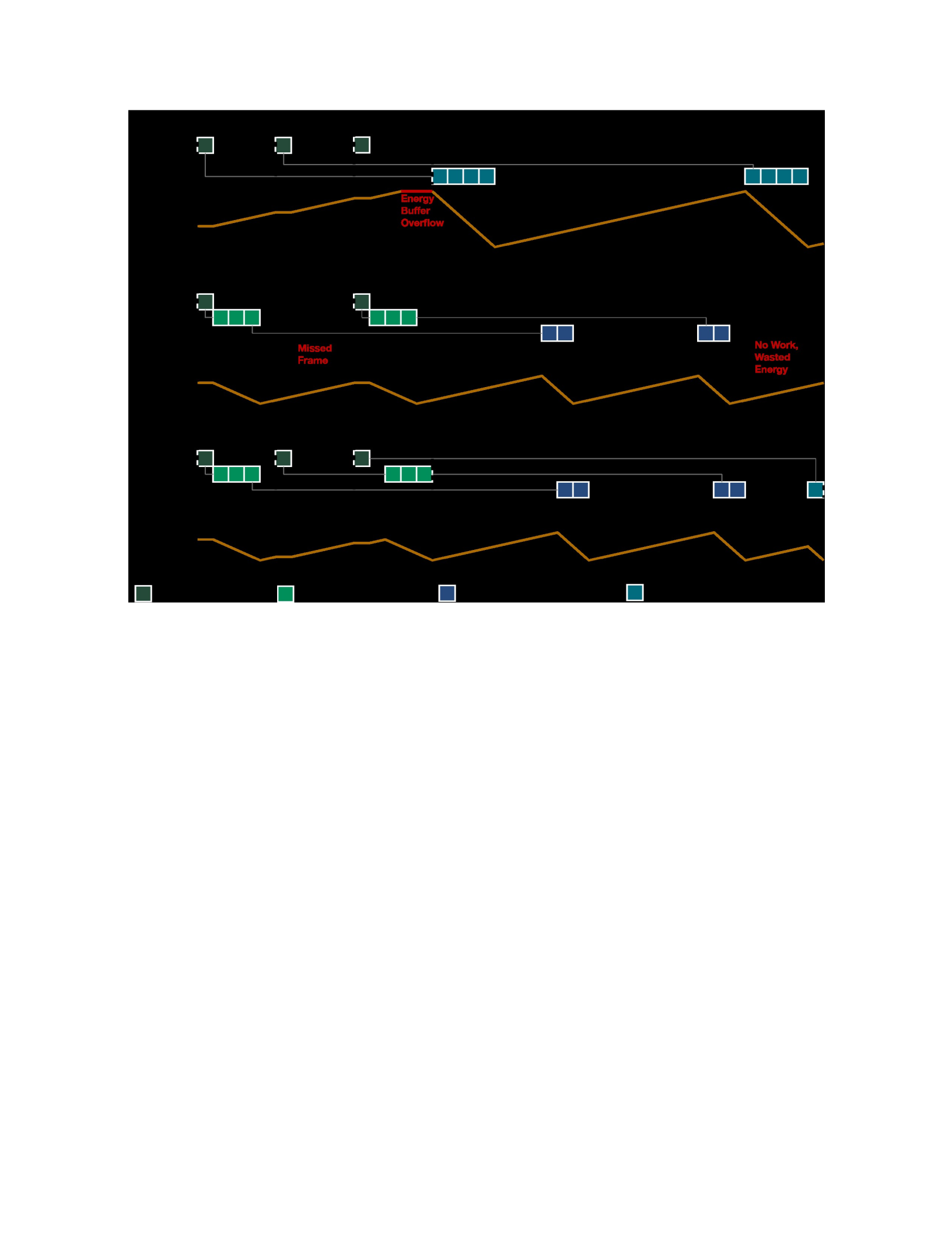
CHAPTER 6. SCHEDULING SATELLITE OPERATIONS 83
Figure 6.6: Top: Bent-pipe scheduling wastes energy. Once the energy buffer fills completely, the satellite loses
additional harvested energy. Middle: Static CNPs provide some benefit. However, without intelligent scheduling,
these devices can miss frames. Bottom: Horizon scheduling provides the best results with energy-aware operation.
olution. However, even with a state-of-the-art embedded processor, the data analysis application often processes
only a small fraction of the total observations. Simply deploying such applications directly to the edge can provide
only limited improvement.
6.3.3 Opportunities with Horizon
Aside from execution time, a factor that limits the benefits from intelligent early discard with orbital edge
computing is energy. Nanosatellites collect a limited amount of energy, and data processing requires high power.
Figure 6.7 illustrates energy usage for both a bent-pipe satellite and a static CNP satellite over the course of one
revolution. With a bent pipe, the majority of the energy is lost due to a full energy buffer and an idle satellite. With
OEC, very little energy is lost. However, the energy is consumed inefficiently.
Horizon makes more efficient use of harvested energy. Depending on the characteristics of the radio and the
processing application, an optimal ratio between data processing and communication can be calculated. In order to
operate at maximum utility, a satellite must dynamically adjust to minimize distance
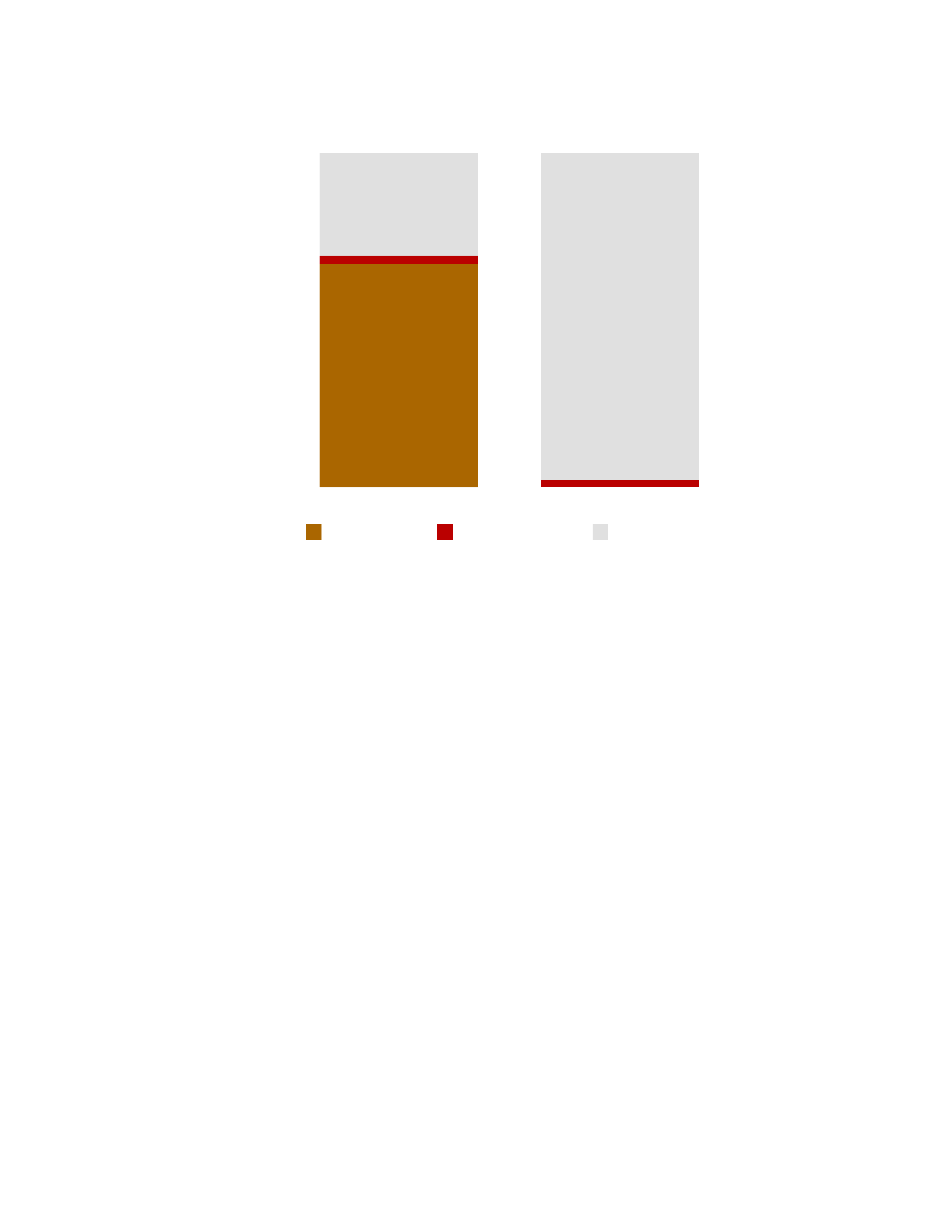
CHAPTER 6. SCHEDULING SATELLITE OPERATIONS 84
Energy per Revolution
Figure 6.7: Left: Bent-pipe satellites lose a majority of harvested energy to energy buffer overflow. Right: With
orbital edge computing, less energy is wasted. However, the energy might not be used efficiently. Horizon is
designed to avoid wasted energy and to allocate energy efficiently.
from this point. Horizon supports this optimization.
A satellite should avoid wasted energy stemming from jobs performed at suboptimal times. With a bent pipe,
satellites cannot react to events. Existing work on orbital edge computing only supports static scheduling. Horizon
allows for new jobs to be added to a system, and it supports dynamic reactions in order to operate at high
efficiency. Horizon is designed to support constraint-focused satellite operations.
6.3.4 Horizon: An Application Narrative
Horizon addresses a challenge of inefficiency in recently-proposed computational nanosatellites [53]. Computational
nanosatellites leverage edge computing in space to improve utility compared to existing nanosatellites, which operate
under a bent-pipe architecture. However, existing proposals are narrowly-scoped to static computational nanosatellite
pipelines that are vertically integrated — the satellite operator and the satellite client are the same. Horizon lays the
groundwork for nanosatellite constellations as a platform in which the satellite operator and the satellite clients are
decoupled.
“Constellations as a service” involve a satellite operator that offers general-purpose Earth-observation services
to clients. Clients may exist on the constellation for extended durations or for brief instants. Such constellations
Kilojoules
0
5
10
15
20
Bent Pipe OEC
Energy Lost Energy Wasted Energy Used

CHAPTER 6. SCHEDULING SATELLITE OPERATIONS 85
begin with satellite operators deploying devices to LEO in a constraints-focused (rather than function-focused)
manner. This strategy allows the operator to service a broad base of clients. Each satellite is characterized by the
operator, and some set of satellite capabilities are exposed (e.g., via an API) to clients for request.
Clients may have many different Earth-observation goals. One client may wish to deploy an app that analyzes
long-term geographic changes; this client’s jobs may persist on constellation satellites for years. Another client may
want to periodically monitor remote infrastructure; this client requires jobs to execute over particular areas
intermittently. Other clients may request a snapshot of a specific area at a particular moment in time, e.g. in
response to a forest fire. With Horizon, all of these clients can easily create a collection of job requests and deploy
them to the operator’s constellation.
The Horizon runtime scheduler uses the operator’s satellite characterizations, client job requests, and real-time
measurements at the edge to select a subset of jobs to execute at each moment. LEO Earthobservation satellites —
especially nanosatellites — are often resource constrained, and a dynamic runtime scheduler is necessary to
maximize device utility. To complete this scheduling task, this work first presents a collection of Horizon concepts in
Section 6.4. It then provides Horizon system details in Section 6.5.
6.4 Horizon Concepts
Horizon is a runtime scheduler that uses real-time measurements, offline operator characterizations, and client job
requests to select a sequence of operating epochs on a satellite system. Horizon consists of a description of
satellite capabilities from the satellite operator, a set of satellite jobs requested by clients, and a runtime scheduler
that selects which jobs to perform based on real-time measurements. These three components operate within a
framework defined by a set of key concepts, including the satellite, its subsystems, and a collection of subsystem
states. Each state exposes a capability that clients request. Clients make requests via job descriptions. Horizon also
defines the concepts of energy buffers, a satellite energy system, data buffers, and a data graph. Figure 6.8
illustrates the Horizon system design.
6.4.1 Modeling the Space Environment
Foundational to the Horizon scheduling approach is simulation of the the space environment. Unlike other energy-
harvesting domains, the space environment is uniquely predictable. In low-Earth orbit (LEO), the environmental
irradiance (i.e. the “solar constant”) is defined to be 1366.1 W/m2[8]. When
Operator Characterizes Virtual Horizon Data Graph
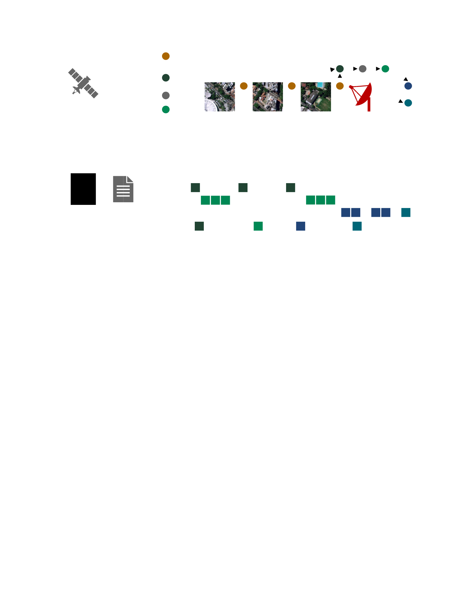
CHAPTER 6. SCHEDULING SATELLITE OPERATIONS 86
Satellite
SubsystemsData
•ADACS
•Sensors
•Processors
•Radio
Client Specifies Jobs Runtime Schedule
•Observe GTFs
•Run App
•Downlink
Figure 6.8: Top left: The satellite operator characterizes satellite subsystems and exposes capabilities for use by
clients. Bottom left: Clients use Horizon tools to describe job requests. Top right: Job descriptions, which request
satellite capabilities, are converted into a data graph. Bottom right: The Horizon runtime scheduler uses real-time
energy measurements to schedule jobs.
the Sun is not occluded by Earth, the amount of power available to harvest by satellite solar panels can be modeled
precisely. Given the solar panel surface area, the solar cell efficiency, and the current-voltage curve of the solar
cells, the available input power can be determined.
Power outages due to eclipse are predictable given orbit characteristics. A typical LEO satellite completes one
revolution around the Earth in roughly 90 min, and less than half of that time is spent in eclipse. This orbit is
defined by the values in the satellite’s two-line element set (TLE). Given the satellite TLE and a date and time, the
standard simplified general perturbation model (SGP4) of orbital mechanics provides a precise location of the
device [99]. The mathematical derivation and a reference implementation of SGP4 are available publicly [99], and
satellite TLEs are posted regularly.
Several software packages exist to model the space environment, including AGI’s STK and the opensource cote
library. Horizon models the space environment with cote because it also models energy, data, and computing
characteristics of satellites. However, Horizon can make use of any software package that provides high-fidelity
simulation and prediction of satellite system states in space (see Section 6.4.4). The space environment model
supports both the Horizon module used by clients to generate jobs (see Section 6.5.2) and Horizon’s runtime
scheduler deployed at the orbital edge (see Section 6.5.3).
d0d1d2
d3dsd4
d5
d6
Nodes
Raw
Data
Operator
Node
Results
Sensor:
Processor:
Radio:
Frame 1 Frame 2 Frame 3 Comm. Session
Observe GTFs Run App Dlink Results Dlink Raw

CHAPTER 6. SCHEDULING SATELLITE OPERATIONS 87
6.4.2 The Energy System
Horizon models the satellite energy system as an energy-harvesting device, an energy-storage device, and a set of
energy-consuming devices. Given a model of both the satellite solar cells and the space environment, the amount of
power available for harvest is well-known. At runtime at the edge, this prediction can be refined by directly measuring
the rate of harvested energy. Horizon uses both techniques to model the energy-harvesting portion of a satellite.
Aside from these energy-harvesting devices, Horizon’s overall energy system model also includes the concepts of
energy-storage devices and energy-consuming devices. A satellite energy system consists of an energy-harvesting
device that provides some amount of power ph during each time epoch, an energy-storage device that contains some
amount of energy E(t) at each time step, and a set of energy-consuming devices that each require some amount of
power pc during each epoch.
Horizon defines an epoch to be a time interval during which the power harvested ph and the power consumed
pc for all energy-consuming devices can be characterized as constant. A change in harvested power or a change in
power consumed by a peripheral results in a new energy-system epoch.
The energy-storage device accepts power from the energy-harvesting device and provides power to the energy-
consuming devices. The energy-storage device has a maximum capacity Emax. The energy-storage device also has a
minimum useful capacity of energy [148]. Below this threshold, no energy-consuming peripheral is able to make
use of stored energy despite the fact that the energy storage device has not been fully drained of Joules. Horizon
scales the amount of energy E contained within the energy-storage device such that E = 0 when this threshold has
been reached. Therefore, ∀t [∈t0, ∞) it is the case that
E(t) [∈0, Emax]
6.4.3 The Horizon Data Graph
Earth-observation satellites collect sensor data, store and process data on orbit, and downlink observations or
results to the ground. The specific data captured and the analysis steps performed depend on the client job
definitions, which are described in Section 6.4.6. These collecting, processing, and downlinking steps define a data
graph, which consists of data-storage nodes, data-operator nodes, and directed edges (representing data transfers)
with corresponding bit rates.
Every data-storage node d is associated with a data-storage device. A data-storage device contains some
number of bits B(t) at each time step. Each device has a maximum capacity Bmax and a minimum capacity of 0. For a
data-storage device D, let the set of associated data-storage nodes be {d0, d1, . . . , dn}. At each time instant,
Bmax. In other words, the number of bits stored in each data-storage

CHAPTER 6. SCHEDULING SATELLITE OPERATIONS 88
node summed across all data nodes associated with the data-storage device must be no greater than the device
capacity.
For example, consider a satellite’s solid-state drive (SSD). Let the data bits of a captured image be associated with
data-storage node d1. Let the data bits output from an image processing application be associated with data-
storage node d2. The sum of the bits associated with d1 and d2 cannot exceed the
capacity of the satellite’s solid-state drive.
Horizon also makes use of “virtual” data storage devices to model sensor data that have not yet been captured.
Suppose a client submits a job to image a particular city. Horizon models this job with a virtual data storage device
associated with a single data-storage node d0. Once the city has been imaged, the data contained in node d0 will
have been transferred to node d1, which is associated with the satellite’s SSD.
Data are transferred (and transformed) between data-storage nodes via data-operator nodes. A dataoperator
node s is associated with a satellite subsystem state; see Section 6.4.4 for details. Each dataoperator node has one
or more incoming edges from data-storage nodes, i.e. data sources, and one or more outgoing edges to data-
storage nodes, i.e. data sinks. Each edge is characterized by an average bit rate r. By definition, all bit rates remain
constant throughout an epoch (i.e. a change in bit rate produces a new epoch). See Section 6.4.2 for a definition of
epoch. When a data-operator node is active, all data sources are drained of bits at the associated bit rate and all
data sinks are filled with bits at the associated bit rate.
6.4.4 Subsystem States
Horizon uses subsystem states to expose satellite capabilities to clients for use in job requests. A state is an
operating mode of a satellite subsystem. A state s must be able to be characterized by an average power draw ps.
This power draw is valid during the state duration [tsmin, tsmax]. Here tsmin is the minimum duration of the state, and
tsmax is the maximum duration of the state. A state is either atomic, in which case it must be scheduled in integer
multiples of tsmin, or it is not atomic and executes for any duration in
[tsmin, tsmax]. Each state has a set of data sources Σs = {σ0, σ1, . . .} and a set of data sinks Ts = {τ0, τ1, . . .};
these are the source and sink data-storage nodes described in Section 6.4.3.
As an example, consider the “capture” state of a camera subsystem. The camera operates in the
“capture” state for a known amount of time ts per frame (e.g. 41.67 ms) — including the readout time. During this
time, a known (e.g., measured) amount of energy Es dissipates on average. Thus, the state power draw ps = Es/ts.
The state duration [tsmin, tsmax] = [ts, ts], and the state is trivially atomic (i.e., the state must endure for exactly ts
seconds). There is one data source, Σs = {σ0}, and one data sink, Ts = {τ0}. For the camera capture state, the bit rate
rσ0 is equivalent to the bit rate rτ0. Both rates are

CHAPTER 6. SCHEDULING SATELLITE OPERATIONS 89
given by the uncompressed bit count per frame divided by the state duration ts.
Other states, like the “nadir” state of the ADACS, may operate for any amount of time. In this case, the state
duration [tsmin, tsmax] = [ϵ, ∞]. Under Horizon, both ϵ and ∞ are system-specific constants (e.g. the minimum and
maximum floating-point values). The state power draw ps is determined through measurement. If the state power
draw fluctuates dramatically, then the satellite operator should split the state definition into multiple states with
consistent power draws. The “nadir” state of the ADACS is not atomic, and both the set of data sources and the set of
data sinks are empty: Σs = Ts = .∅
An object-detection convolutional neural network (CNN) is a non-trivial example of an atomic state. Each
execution of the CNN requires an input image, a well-defined amount of time (e.g. 44.86 ms), and energy (e.g.
0.5069 J). Without adding the ability to checkpoint and pause the CNN’s execution, the workload must execute
atomically — i.e., in 44.86 ms increments. Non-integer multiples of the minimum duration waste work because an
image is partially processed and the computation is abandoned before producing a result. Thus, the state duration
[tsmin, tsmax] = [tsmin, ∞]. There is one data source, Σs = {σ0},
and one data sink, Ts = {τ0}. The data source contains images with a bit rate given by the size of an image divided by
the duration of the atomic execution. The data sink contains bounding box outputs, resulting in bit rate at least one
order of magnitude smaller than the input bit rate.
6.4.5 Subsystems and the Satellite System
A satellite subsystem is defined by its set of subsystem states. The satellite operator is responsible for selecting
which subsystem states to expose to clients. For example, the satellite operator might expose the “off” and “nadir”
states of the satellite ADACS for client use. The satellite operator might expose the “idle” and “capture” states of
the satellite camera, and the “off,” “transmit unprocessed data,” and “transmit processed data” states of the radio
transmitter. Each state request is then arbitrated by the Horizon runtime scheduler.
In Horizon, a satellite system consists of all satellite subsystems together with one or more data-storage devices
and an energy-storage device. The harvested power is determined at each time step according to Section 6.4.2. The
harvested power, energy storage, and subsystems (i.e., the energy-consuming devices) compose the satellite
energy system.
6.4.6 Client Jobs
Horizon clients create job requests that are deployed to satellites for scheduling. A client job includes a start time
t0, a cease time t1, and a set of required states R = {s0, s1, . . . , sn}. The job start time and cease time define an
interval [t0, t1) during which the job is considered schedulable. While a job is schedulable, the Horizon runtime

CHAPTER 6. SCHEDULING SATELLITE OPERATIONS 90
scheduler considers the job for execution. Otherwise (i.e. t [∈ t0, t1)), Horizon does not consider the job for
execution. Note that [t0, t1) defines the interval during which the job may begin
Figure 6.9: Clients create job requests with Horizon. The Horizon simulator converts these time requests into time
intervals for the target satellite. These jobs are then deployed to the edge for runtime scheduling according to
energy availability.
execution; after being scheduled, the job may persist beyond t1.
In order to schedule the job, the satellite must operate with all required states R = {s0, s1, . . . , sn} active. For
example, a client job requesting an image of a particular ground track frame must require the camera system to
operate in the “capture” state and the ADACS to operate in the “nadir” state. If the Horizon runtime scheduler can
meet these requirements, then the job may be scheduled. Recall from Section 6.4.4 that each state contains
multiple operating conditions (e.g. minimum and maximum durations, atomicity requirements, and data source
and sink nodes). Horizon’s system-level synthesis of these requirements are described in Section 6.5. Figure 6.9
illustrates client job requests in Horizon.
6.5 Horizon System Design
Horizon is composed of three major components. First, the operator characterizes satellite capabilities as a
collection of subsystems, each with a finite set of operating states. Section 6.5.1, the “Operator Description,”
describes this component. Second, the customer or client wishing to leverage satellite capabilities submits a
collection of jobs. Using Horizon’s job-generation tools, the client specifies when during the satellite orbit the job
may begin and what capabilities are required to complete the job. Section 6.5.2, the “Client Requests,” describes
this component. Third, the Horizon runtime scheduler utilizes the operator description, the client requests, and
real-time system measurements to select a set of jobs to schedule concurrently during each epoch. Section 6.5.3,
the “Runtime Scheduler,” describes this component.
6.5.1 Operator Description
In order to support Horizon scheduling, the satellite operator must enumerate the satellite subsystem capabilities.
Subsystems may be enumerated at any granularity. In the case of nanosatellites, this work selects a coarse-grained
subsystem enumeration: the attitude determination and control system (ADACS), the camera sensor system, the
radio systems, and the data processing system. This coarse-grained enumeration is sensible for energy-constrained
nanosatellites, because each of these subsystems draws power of the same order of magnitude as the rate of

CHAPTER 6. SCHEDULING SATELLITE OPERATIONS 91
harvested energy. Other applications may require a fine-grained subsystem enumeration, e.g. enumerating each
functional block in a CPU as a separate subsystem.
After choosing a granularity and enumerating the satellite subsystems, the satellite operator must identify a set
of operating states for each subsystem. The set of operating states defines which capabilities are exposed for client
use. Therefore the set of operating states need not be exhaustive, but it must include any capabilities that the
satellite operator wishes to expose to clients. Under our coarse-grained example, the ADACS provides “off” and
“nadir” operating states. The camera offers “idle” and “capture” operating states, and the transmit radio offers
three states: “off,” “transmit unprocessed data,” and “transmit processed data.”
Subsystem operating states act as a description of the subsystem capabilities and constraints for the Horizon
scheduler. Each state defines a collection of properties determined via offline characterization. These properties
include the subsystem power draw while operating in each state, the minimum and maximum state duration, and
data production and consumption rates. States that require a precise amount of time (e.g. a camera sensor
capturing an image) set the maximum state duration equal to the minimum state duration. States that can persist
for arbitrary durations (e.g. an ADACS in nadir mode) set the minimum duration to “epsilon” and the maximum
duration to “infinity.” States that progress in atomic steps (e.g. an image processing application without
checkpoints) set a minimum duration (e.g. the processing time of a single image) and no maximum duration. An
“atomic” flag indicates that the state should be scheduled in atomic increments.
6.5.2 Client Requests
Horizon’s job-specification tools allow each client to request use of subsystem states in order to leverage satellite
capabilities. These tools expose to the client the satellite capabilities as specified by the satellite operator and
translate client jobs into the format required by the Horizon scheduler. For each job, the client selects any required
subsystem states. A client job to image a particular ground track frame must require the camera system to operate
in the “capture” state and the ADACS to operate in the “nadir” state. Because this frame is visible only during
certain time intervals, the job must specify a period during which it could be successfully scheduled. This time
interval [t0, t1) is generated for the client using Horizon tools. Therefore, each job is considered to be schedulable
during the interval of time [t0, t1) and
unschedulable otherwise.
Before deployment to the edge, all jobs from all clients are sorted (earlier first) by their schedulable start date
and time t0. In the case of ties, jobs are sorted (earlier first) by their schedulable cease date and time t1. As a result,
all jobs with schedulable intervals containing the current date and time are easily selected at run time.

CHAPTER 6. SCHEDULING SATELLITE OPERATIONS 92
6.5.3 Runtime Scheduler
Given the system capabilities, the client jobs, and real-time system measurements, the Horizon scheduler selects a
set of jobs to schedule concurrently during each epoch. Real-time system measurements include the rate of
harvested energy, the amount of energy available in the energy buffer, and the amounts of onboard buffered data.
Horizon produces schedules as a sequence of epochs. An epoch is any duration of time during which the
satellite state does not change, i.e. the harvested power remains consistent and the satellite subsystem states do
not toggle. Thus, predictable changes in harvested power trigger a new epoch. Other than a change in harvested
power, a new epoch begins when an energy buffer or a data buffer is depleted or filled, or when a state duration
expires.
Horizon schedules a set of jobs for execution during each epoch [t0, t1). The epoch start time, t0, is known.
Therefore, the challenge for Horizon at each epoch is to determine both the set of jobs to schedule and the cease
time t1 of the epoch.
6.5.4 Epoch Schedule Selection
The Horizon runtime scheduler performs a sequence of steps in order to determine which set of jobs to select during
each epoch. First, Horizon collects all schedulable jobs given the current date and time. Recall that a job is considered
to be schedulable if the current date and time is within the time interval [t0, t1) during which the job is allowed to
start. From this set of schedulable jobs, Horizon generates all job sets. Horizon then prunes any job sets with
conflicting state requirements. Using the power, data, and timing requirements of each job, Horizon also prunes any
job sets that cannot complete under the current system state (e.g. harvested power, stored energy, or stored data).
Finally, Horizon ranks the remaining job sets by utility and selects one job set to schedule for the epoch. A more
detailed description of each step is provided in the following subsections.
Collect Schedulable Jobs: Recall that each job includes a time interval [t0, t1) during which the job is allowed to
start. This interval is specified by the client while generating the job description with the help of Horizon tools. For
example, in order to image a particular ground track frame the “capture” job must begin while the satellite is over
the region of interest. A client specifies this region of interest, and the Horizon client tools produce the time
interval during which the region is visible. Therefore, at each moment in time, only some subset of jobs are
schedulable. As a first step, the Horizon runtime scheduler identifies these schedulable jobs as candidates for
execution during the next epoch. If it exists, Horizon also identifies the next unschedulable job for later use.
Generate All Job Sets: Given a set of schedulable jobs, the Horizon runtime scheduler must select some subset
of jobs for concurrent execution during the next epoch. As a first step, Horizon generates all possible combinations
of the schedulable jobs. For example, if three jobs (A, B, and C) are schedulable during the next epoch, then

CHAPTER 6. SCHEDULING SATELLITE OPERATIONS 93
Horizon generates eight possible combinations: the individual jobs {A}, {B}, and {C}; the job pairs {A, B}, {A, C},
and {B, C}; all jobs running concurrently {A, B, C}; and no client jobs running {}. Each job set is characterized by the
required subsystem states (the union of the required subsystem states for each individual job), the maximum of all
minimum state durations (i.e. the minimum duration of the job set), and the union of all data sources and data
sinks among the jobs in the set.
Prune Conflicting Requirements: Recall that each job includes a set of required states. For example, to image a
particular ground track frame, the satellite ADACS must be active to point the camera, and the satellite camera
must operate in the image capture state. If two schedulable jobs require the same subsystem to operate in
different states, then those jobs cannot be scheduled simultaneously. The Horizon runtime scheduler prunes any
such job sets from consideration.
Prune Infeasible Job Sets: Horizon makes use of real-time measurements and state characteristics to eliminate
infeasible job sets. Horizon determines the maximum duration of the job set by calculating the minimum of all
maximum job durations. If the maximum duration of the job set is less than the minimum duration of the job set,
then the job set is rejected as infeasible. A job set is also rejected as infeasible if the energy buffer would deplete
before the minimum duration of the job set, if any data source would deplete before the minimum duration of the
job set, or if any data sink would overfill before the minimum duration of the job set.
Refine Maximum Duration: Of the remaining (feasible) job sets, the maximum duration of each set must be
refined. Previously, the maximum duration of each job set was calculated as the minimum of all maximum
durations of each individual job. If executing the job set for this duration would deplete the energy buffer, then the
maximum duration is shorted to the time to deplete the buffer. If executing the job set for this new maximum
duration would exhaust a data source, then the maximum duration is shortened to the time to deplete the source.
If executing the job set for this new maximum duration would overfill a data sink, then the maximum duration is
shortened to the time to fill the sink. If any of the jobs execute atomically, then the maximum duration is decreased
to support an integral number of atomic executions.
Determine Job Set Utility: Efficient job sets avoid energy buffer overflows. When both efficient and inefficient
job sets remain, Horizon selects from the group of efficient job sets. If no efficient job sets remain, then Horizon
selects from the group of inefficient job sets. Horizon selects the job set with the highest utility. This work
implements a utility function designed to produce the highest number of data sink bits. During deployment, the
satellite operator chooses the utility function to best support the device use case.
Schedule a Job Set: Horizon selects the efficient job set with the highest utility. If no efficient job set exists,
Horizon selects the inefficient job set with the highest utility. An efficient job set is scheduled for its maximum
duration. An inefficient job set is scheduled until the next unschedulable job becomes schedulable or for its

CHAPTER 6. SCHEDULING SATELLITE OPERATIONS 94
minimum duration. If the trivial, “all off” job set is scheduled, then the duration continues until the next
unschedulable job becomes schedulable.
Prepare for the Next Epoch: When a one-time job is scheduled, it depletes its virtual data source and therefore
will not be eligible to be rescheduled. After execution of an epoch, the energy and data buffer values are updated.
Given the new date and time, the schedulable jobs list is re-calculated and the Horizon runtime schedule selects a
new job set for execution during the next epoch.
6.6 Methodology
For evaluation, this work implements an operator description, a collection of client job requests, and the Horizon
runtime scheduler. The operator description provides clients with a state-of-the-art nanosatellite equipped with
commercial, off-the-shelf (COTS) satellite components. These components include an ADACS, a camera sensor, a
radio, and a computing module with an embedded GPU for accelerating machine inference workloads [177, 2, 213,
104, 11]. In order to evaluate the ability for Horizon to make use of satellite hardware with different energy
efficiencies, this work varies the radio module. This work examines commercially available UHF, S-Band, and X-Band
satellite radios [109, 84, 108, 113, 114].
The client job requests use cote to produce a sequence of GTF image requests across a satellite orbit. The orbit
matches that of a deployed, Earth-observation nanosatellite. The client workload captures the images, performs
CNN processing, and downlinks the result. On average, the CNN output (pixels in bounding boxes indicating
features of interest) is ten times smaller in data volume than the input images. In order to evaluate the ability for
Horizon to adjust to different CNP constellation populations, this work adjusts the number of tiles per frame that
the satellite is responsible for processing.
The Horizon runtime scheduler is implemented using the Python scripting language. Emerging cubesats [161]
and even chip-scale [267] satellites support onboard interpretation of Python scripts. For additional optimization,
the runtime scheduler may be implemented in C and incorporated into an embedded operating system. Such an
implementation would be ideal for emerging nanosatellite platforms [148].
6.7 Evaluation
This work compares the Horizon scheduler against the previous state-of-the-art: static computational nanosatellite
pipelines (static CNPs). In order to evaluate the benefits of Horizon, this work considers three variables. First, it
considers the amount of data each satellite is responsible for processing. Under the static CNP proposal, each
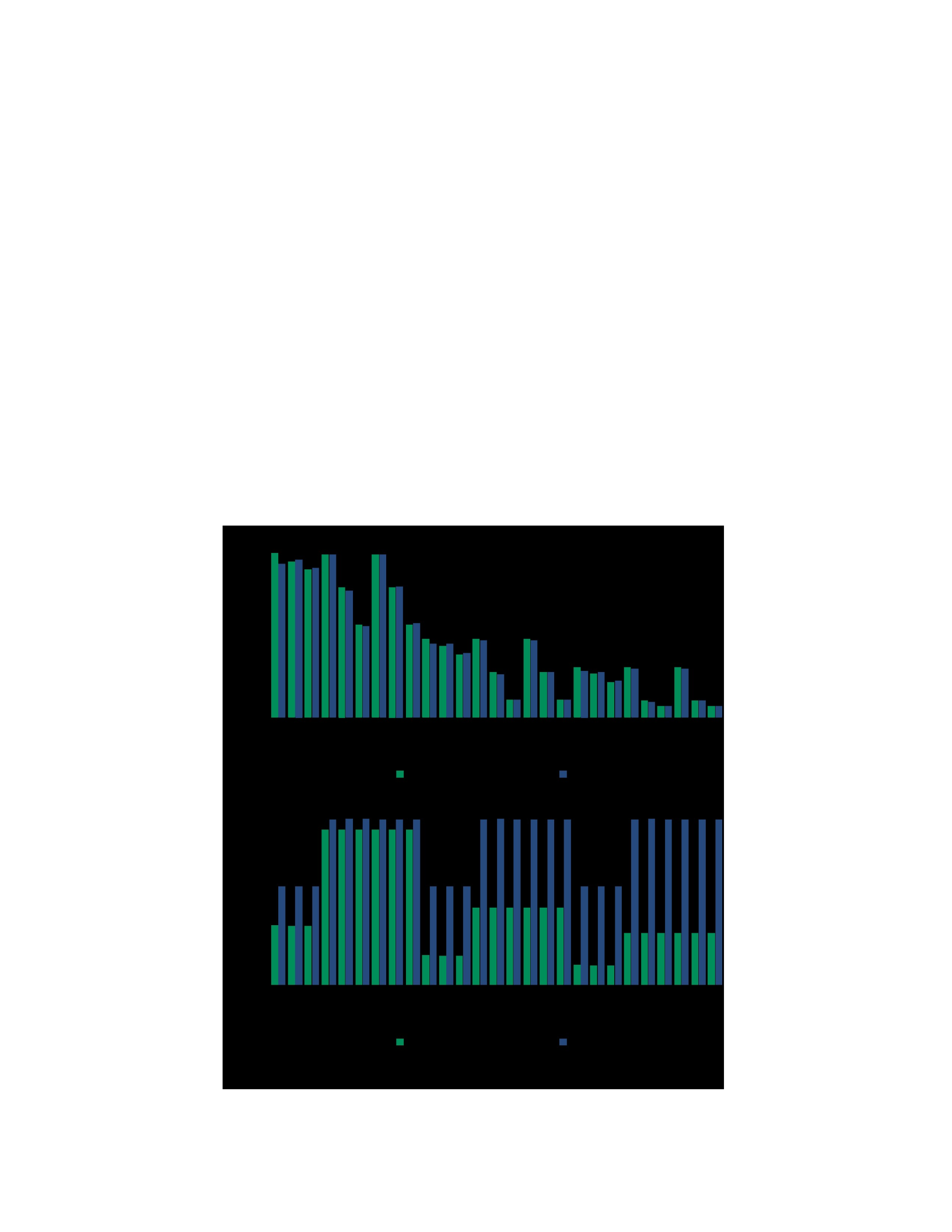
CHAPTER 6. SCHEDULING SATELLITE OPERATIONS 95
satellite captures an image and processes a subset of tiles. This work considers the cases in which the satellite is
responsible for processing all tiles, half of the tiles, and one third of the tiles.
It also considers the amount of power harvested by each satellite. Nanosatellites have limited solar panel
surface area, resulting in limited energy budgets. Designers achieve increased solar panel surface area, and
therefore increased harvested power, with deployable solar panels. Deployable solar panels increase cost and risk
— two factors that nanosatellites avoid. This work evaluates surface-mounted solar panels, two sets of deployable
panels, and four sets of deployable panels.
Nanosatellites often utilize UHF, S-Band, or X-Band radio. UHF provides the lowest bit rate, S-Band provides a
higher bit rate, and X-Band provides the highest bit rate. In general, higher bit rates require more power
consumption. However, the energy consumed per bit transmitted depends on the particular radio module. Some
COTS radios with high bit rates are less energy-efficient than COTS radios with lower bit rates. This work evaluates
three COTS nanosatellite radio modules: UHF, S-Band, and X-Band.
For each configuration, this work compares the static CNP results with the Horizon results. This work
Figure 6.10: Top: The amount of unprocessed data remaining on the satellite is similar for both the static CNP
baseline and the Horizon scheduler. Bottom: The amount of processed data remaining on the satellite is greater
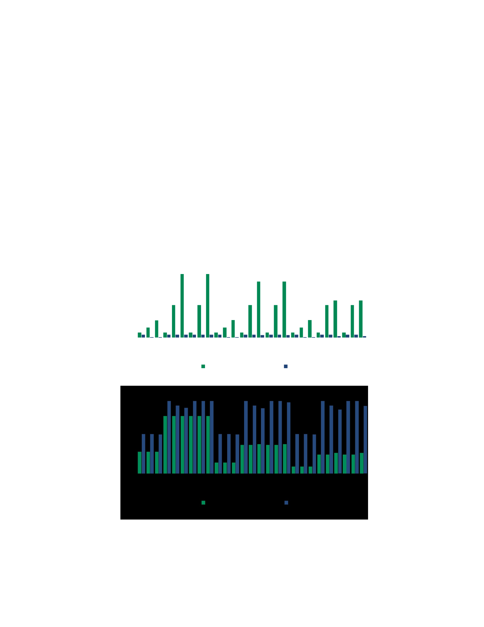
CHAPTER 6. SCHEDULING SATELLITE OPERATIONS 96
with Horizon than with the static CNP baseline. This change shows that the Horizon scheduler processes data more
efficiently.
compares four measurements. First, it considers unprocessed data on orbit. This measure illustrates the amount of
data collected by the satellite that is neither processed nor downlinked by the end of the revolution. Next, it
considers processed data on orbit. This measure illustrates the amount of data collected and processed by the
satellite but not downlinked before the end of the revolution. This work then considers unprocessed data and
processed data downlinked. Better-performing satellites downlink more processed data and less unprocessed data.
6.7.1 Data on Orbit
This work considers the amount of unprocessed and processed data remaining on the satellite after one revolution.
These measures provide insight into the relative time and energy spent by the static CNP base-
Unprocessed Data Downlinked
Processed Data Downlinked
D3: 1/3 Image P3: 15U Solar Array R3: X-Band Radio
Figure 6.11: Top: The amount of unprocessed data downlinked is dramatically lower in the case of the Horizon
scheduler because Horizon is able to prioritize data processing. Bottom: Horizon downlinks more processed data
compared to the static CNP baseline.
D1 D2 D3
P1 P2 P3 P1 P2 P3 P1 P2 P3
R1 R2 R3 R1 R2 R3 R1 R2 R3 R1 R2 R3 R1 R2 R3 R1 R2 R3 R1 R2 R3 R1 R2 R3 R1 R2 R3
Data (MB)
0
600
1200
1800
2400
3000
Static CNP Horizon

CHAPTER 6. SCHEDULING SATELLITE OPERATIONS 97
line and the Horizon scheduler on data processing. The static CNP baseline captures ground track frames and
processes tiles until arriving near a ground station. During a communication session, the satellite downlinks
processed and unprocessed data. A static CNP cannot react to real-time energy measurements. The Horizon
scheduler dynamically selects jobs to execute at each time epoch.
For all configurations, the static CNP baseline and the Horizon scheduler collect similar amounts of unprocessed
data on orbit. These results can be seen in Figure 6.10, top. These measurements represent the amount of
unprocessed data remaining on the satellite after one revolution. As harvested power increases, the amount of
unprocessed data decreases because more energy is available to process and downlink data. Higher bit rate radios
also decrease the amount of unprocessed data remaining in orbit because more data is downlinked during the
limited communication session.
The amount of unprocessed data on orbit increases under Horizon scheduling compared to static CNPs. Horizon
scheduling prioritizes data processing within energy constraints. Horizon also makes better use of limited energy,
resulting in more processed data. The amount of processed data increases as the harvested energy increases
because more energy is available to operate the onboard processor.
6.7.2 Data Downlinked
This work also considers the amount of unprocessed and processed data downlinked from the satellite after one
revolution. These measures provide insight into the overall effectiveness of each approach in downlinking data for
ground use. The static CNP baseline captures ground track frames and processes tiles until arriving near a ground
station.
The Horizon scheduler downlinks dramatically less unprocessed data per revolution. The Horizon scheduler
prioritizes data processing and reacts dynamically to energy availability in order to make the most efficient use of
energy. As a result, more energy is spent processing data and downlinking processed data. This effect can be
observed in Figure 6.11, bottom. In all cases, Horizon downlinks more processed data compared to the static CNP
baseline.
6.8 Related Work
This work spans computer systems, space systems, energy-harvesting, and device operations. Section 6.1 provides
a brief space systems background. Recent edge computing work provides context for this work. Edge computing
recognizes that, as high-datarate sensors (e.g. cameras, lidar) proliferate, streaming all data to central cloud
systems for processing becomes infeasible [199, 198]. Intermittent computing [149] shares challenges with orbital
edge computing in that both types of systems are fully energy-autonomous. Works like CatNap [157] and Chinchilla

CHAPTER 6. SCHEDULING SATELLITE OPERATIONS 98
[155] explore scheduling for intermittent systems without the benefit of a modelable space environment. While
similar in spirit, these efforts differ significantly in scale, deployment environment, and in their inability to rely on
processor sleep modes; instead, they power off frequently. Horizon focuses on energy-aware satellite scheduling
and operations in the space domain, but extensions of Horizon are expected to be generally applicable to energy-
constrained computer system operations.
While many works have examined oversubscribed, highly-constrained scheduling problems, the space domain
lends itself to a unique approach. Datacenters assume an unpredictable influx of jobs and are forced to make use of
probabilistic models and solutions. In some drone domains, limited physical modeling of the environment is
possible. However, drones by definition are deployed into unknown and, to some degree, unpredictable
environments. LEO Earth-observation satellites operate in a unique domain. The time an location of every
observation is known far in advance. With client job requests under Horizon, the possible actions taken at these
times and locations are also well-known. Horizon leverages the unique predictability of the space environment to
efficiently schedule device job requests.
6.8.1 Schedulers for Computer Systems
Recent computer system scheduler works focus on datacenters, clusters, and servers. RackSched [271] observes
that datacenters provide low-latency support to online services with rapid adjustment of multicore resources —
i.e., elastic resource scaling. After showing both the need for and the challenge of such low-overhead scaling across
servers (instead of within a server), RackSched presents a two-layer framework for “super” elastic scaling across a
rack. RackShed quickly assigns incoming requests to workers with a goal of high throughput and low latency.
Horizon uses characterization, physics-based modeling, and telemetry, along with an operator description of the
satellite system and client job requests, to place system devices into a sequence of operating states maximizing
useful results delivered to clients. For a constellation of satellites, clients must provide job requests well in
advance; Horizon need not assign requests to workers within microseconds.
As a key feature, Horizon generates a satellite constellation schedule by reasoning about communication,
computation, energy, and other constraints. Wing [40] makes a related observation for computer cluster jobs: while
a majority of such jobs depend on the results of other jobs, many cluster schedulers lack awareness of these
dependencies. The Horizon data graph (Section 6.4.3) expresses dependencies similar to those observed by Wing,
where jobs or tasks consume bits produced by other, independent jobs or tasks. Unlike Wing, which depends solely
on characterization of historical dependencies via logs, Horizon enforces explicit specification of dependencies.
Gavel [173], a scheduler for deep neural network (DNN) training in clusters, recognizes that existing systems
lack awareness of different application performance on heterogeneous accelerators. To remedy this shortcoming,

CHAPTER 6. SCHEDULING SATELLITE OPERATIONS 99
Gavel incorporates this knowledge into the scheduling process. Despite the recent focus on energy and power in
accelerator computer architecture research and the growing focus on energy and power for datacenters, Gavel
does not consider either of these factors. Horizon considers energy as a primary constraint, along with other
interdependent and potentially blocking constraints such as communication and data availability.
Satellite constellations, particularly when acting as a platform to which third-party clients deploy applications,
experience resource limitations and are therefore inelastic. Many cluster schedulers, including Pollux [185], make a
fundamental assumption of elasticity. Pollux adds or removes resources to promote DNN training throughput while
maintaining “statistical efficiency,” a metric unique to deep learning. This insight supports shifting resources away
from a job during portions of the job lifetime. Horizon coschedules client job requests to maximize the utility of the
constellation for the operator by delivering the most useful data to the ground segment.
PrivateKube [150] extends the Kubernetes container manager to account for a global privacy resource that does
not replenish when training ML models with differential privacy. Other resources managed by Kubernetes, such as
CPU or GPU devices and memory, do replenish after job completion. Horizon models CPUs and GPUs as device
subsystems that consume resources like time, energy, and data to produce outputs. Subsystem states represent
applications, and Horizon identifies when and in what order these states begin and end.
Cluster schedulers commonly allocate GPUs for DNN jobs and associate fixed amounts of CPU and memory
resources per GPU. Synergy [169] observes that some DNN jobs receive excess CPU and memory resources under
this scheme. Worse, other DNN training jobs experience “data stalls” due to a lack of CPU or memory resources.
Horizon expands such an observation to a first-class concern. Clients specify dependencies between tasks so that
the Horizon scheduler can minimize both data stalls and, new to this work, analogous “energy stalls.”
Gavel, Pollux, PrivateKube, and Synergy all focus on deep learning and neural network training aspects of
cluster scheduling. These applications represent a narrow but topical set of datacenter workloads. Similarly,
Horizon focuses on evaluation of client job requests composed of machine inference tasks and supporting,
computer-vision tasks that dominate the Earth-observation, computational nanosatellite literature.
Other scheduling work focuses on automatic selection of sparse tensor kernel execution strategies while
keeping the search space small [3]. Finding an asymptotically advantageous execution schedule requires balance
between both the accuracy and the complexity of the execution model; for example, the authors omit modeling
cache effects. Horizon balances the accuracy and complexity of physics-based models. Unlike static autoscheduling
[3], Horizon incorporates system telemetry for schedule updates.
For hardware, a recent work [66] generates a streaming accelerator with minimal area that meets a
programmer-defined throughput threshold. While the work does describe hardware design trends toward energy

CHAPTER 6. SCHEDULING SATELLITE OPERATIONS 100
efficiency, the system does not directly optimize for power or energy. Horizon explicitly minimizes wasted energy to
improve system performance.
CatNap [157] schedules tasks on an embedded computer executing intermittently due to frequent power
outages. Targeted at terrestrial remote sensors harvesting energy from the environment, CatNap faces
unpredictable energy availability. This system aims to support event-driven applications with unpredictable arrival
times. Horizon benefits from a domain with high predictability; in space, both energy and event arrival are known.
In LEO, a well-known constant [8] characterizes solar irradiance, and no clouds obscure the Sun. Orbital mechanics
provide target acquisition times. Horizon leverages characterization, physics-based models, and telemetry to avoid
the failure scenarios addressed by CapNap.
6.9 Summary
This work develops Horizon: a system for dynamically scheduling satellite operations in order to improve support
for edge computing in space. As LEO proliferates with new constellations of satellites, historical approaches to
space vehicle (SV) management break down. Bent-pipes struggle with a downlink bottleneck, and recent proposals
for static OEC cannot react to dynamic satellite states. In order to make better use of satellite systems, this work
proposes a new system for satellite operations. Using satellite operator characterization, client job requests, and
real-time measurements at the edge, Horizon dramatically improves device utility.

Chapter 7
Designing and Manufacturing a Picosatellite
Large, expensive, monolithic satellites dominate low-Earth orbit (LEO) Earth observation. Space vehicles (SVs) like
WorldView-3 [74], Earth-Observing 1 [168], and Landsat-8 [144] cost hundreds of millions of dollars each [91] and
require over a dozen years of “arduous” development [144]. To justify such time and expense, these SVs must
operate for decades. Extremely high cost demands extremely low risk; as a result, designers often select satellite
subsystems for their “flight heritage” and not for their cutting-edge capabilities. By the end of a satellite mission,
some components may be more than a quarter century
behind the state-of-the-art.
Monolithic, expensive satellites usually take this approach. For these satellites, a ground segment closely
manages operations via a bent pipe [136]: ground stations transmit commands to the satellite, and the satellite
responds with raw, unprocessed sensor data. Innovation often concentrates around the sensor payload of these
monolithic, expensive satellites. Generally, these systems perform minimal onboard computing [38, 6, 19] and
instead focus on reliable remote control from the ground.
Recently, there has been a proliferation of LEO launches with nanosatellites. A typical nanosatellite is four
orders of magnitude cheaper, three orders of magnitude less massive, and four orders of magnitude smaller than a
typical, monolithic satellite. Rather than operate for decades, a nanosatellite operates for a few years at most or a
few weeks at least. Lower costs and shorter missions reduce per-device risk and support use of cutting-edge,
commercial, off-the-shelf (COTS) hardware. If hardware lacking flight heritage fails, the nanosatellite can be quickly
replaced.
Higher per-device risk tolerance of nanosatellites provides opportunities to deploy more advanced subsystems
to orbit compared to expensive, monolithic satellites. However, most nanosatellites still adhere to the same
concept of operations (CONOPS) as monolithic satellites; i.e., a bent pipe [61]. New Earthobservation capabilities
enabled by large constellations — e.g., daily global coverage — are limited by
106
continued adherence to a bent-pipe CONOPS [138]. Additionally, new challenges — e.g. effectively managing a large
constellation by remote control [138] — arise in a more crowded LEO.

CHAPTER 7. DESIGNING AND MANUFACTURING A PICOSATELLITE 102
Recent work observes, enumerates, and characterizes some of these challenges [52, 53, 148]. For example, a
proliferated LEO exacerbates the downlink bottleneck: Earth-observation satellites and constellations observe much
more data than can be downlinked per orbit revolution. These challenges are addressed by orbital edge computing
(OEC): colocating computing resources with sensors on orbit to process data before transmission. OEC makes better
use of limited communication opportunities by pre-processing and selecting valuable data for transmission.
However, this technique generally requires significant energy for computation on the satellite.
Thus, the volume and surface area constraints of nanosatellites make OEC particularly challenging to deploy.
Limited surface area and low-cost requirements prevent nanosatellites from leveraging overprovisioned solar
panels. Limited volume constrains the amount of energy that can be stored inside the device (i.e., the capacity of
the energy buffer). This work imports techniques of intermittent computing from cutting-edge computer systems
research to reconcile the benefits of OEC with the constraints of a nanosatellite platform. energy is buffered with a
supercapacitor instead of a battery — a choice that is further motivated in Section 7.1.2.
Because evaluating all proposed OEC schemes in orbit is not practical, previous work developed the cote
software library to assess proposals in simulation [53]. TA1 integrates with cote and any other space simulation
environment via TAB to provide a hardware-in-the-loop evaluation platform. This work presents a low-cost, open-
source [55, 56] satellite to augment simulated OEC evaluation with both hardware-in-the-loop (before launch) and
in orbit (after launch).
Tartan Artibeus (TA1) is an open-source hardware [55] and software [56] pocketqube satellite for OEC research.
Figure 7.1 provides exterior and interior views of TA1. The TA1 command and data handling (C&DH) module serves
as an arbiter between standard subsystem modules and the batteryless electrical power system (EPS), which
harvests energy into a supercapacitor. To abstract the batteryless, intermittent operation from other subsystems,
TA1 introduces the Tartan Artibeus Bus (TAB): a framework for integrating independently-developed satellite
subsystem modules. TAB extends the open-source OpenLST [130] serial communication protocol to support OEC
operations. The C&DH module uses TAB to operate satellite subsystems oblivious to the batteryless, intermittent
nature of the satellite. Further, TAB supports integration with external simulation tools like cote for hardware-in-
the-loop evaluation. TA1 leverages TAB to provide an open source platform for OEC research.
In summary, Tartan Artibeus provides the following contributions to computational space systems research: (i)
TA1 complements software-based OEC simulation with a batteryless, hardware platform
(a) TA1 Assembled. (b) TA1 Board Stack.
Figure 7.1: TA1 Satellite. TA1’s modular stacking design (visible at right in a prototype) easily integrates new payloads.

CHAPTER 7. DESIGNING AND MANUFACTURING A PICOSATELLITE 103
for real-world evaluation; (ii) TAB provides a communication framework for easy integration of flight hardware with
both software simulation environments and new hardware research modules (e.g. experimental payloads); (iii) TA1
is an open-source hardware [55] and software [56] reference implementation of a flight-ready picosatellite for in-
situ OEC evaluation; and (iv) TA1 software includes three reference apps that exercise TAB and provide a model for
OEC research CONOPS.
7.1 Background
LEO satellite systems proliferate as new launch services [78] provide increasing access to space. Nanosatellite
deployments in particular exhibit rapid growth [225] since the standardization of the “cubesat” form factor [167].
Satellites continue to reduce in size with the recent proposal of the “pocketqube” standard [186] and deployments
of “chipsats” [267]. This work provides an overview of existing LEO nanosatellites, opportunities to leverage
batteryless and intermittent computing in space, and the emerging field of orbital edge computing (OEC).
7.1.1 Existing Nanosatellites
Smaller satellite sizes and costs support deployments of large numbers of devices to LEO. For the first time, satellite
constellations consist of hundreds of devices [29, 138] instead of dozens. Now, some of the largest LEO
constellations consist almost entirely of nanosatellites. A nanosatellite masses between 1 kg and 10 kg. Often, a
nanosatellite adheres to the cubesat standard [167] to leverage COTS components and launch services.
Momentum toward even smaller designs, like the pocketqube standard [186], promise even lower unit costs.
While a cubesat consists of integer multiples of 10 cm×10 cm×10 cm (“1U”) volumes, and each 1U volume
must mass no more than 1.33 kg, a pocketqube consists of integer multiples of 5 cm ×5 cm×5 cm (“1p”) volumes.
Each 1p volume of a pocketqube must mass no more than 0.25 kg (i.e., 250 g). Thus, even a 3p pocketqube cannot
meet the 1 kg threshold to be considered a nanosatellite and might more accurately be described as a picosatellite.
Satellites smaller than a picosatellite — i.e., a chipsat — may be even cheaper to launch in high quantity, but they
do not yet enjoy the benefits of standardized COTS components and launch services.
For decades, universities and other education-focused organizations launched and operated the majority of LEO
nanosatellites. More recently, multiple business organizations [29, 138] have deployed large nanosatellite
constellations for commercial Earth-observation. These constellations enable new geospatial applications — e.g.,
observing the entire Earth in a single day [138]. However, effectively managing satellites by remote control — i.e.,
via a bent-pipe — grows increasingly difficult with larger constellation populations [138].
The smaller size of emerging satellites creates new challenges. Nanosatellites face exacerbated downlink
bottlenecks [53], limited data quality due to volume constraints [52], and less harvested power [148]. In contrast,

CHAPTER 7. DESIGNING AND MANUFACTURING A PICOSATELLITE 104
monolithic satellites enjoy large engineering margins for power. These systems may harvest more than 3 kW via
solar arrays. A 3U nanosatellite with low-risk, body-mounted solar panels harvests less than 10 W of power —
three orders of magnitude less than a large SV. Picosatellites and chipsats face more stringent power budgets. As
satellites become smaller, their design must address increasingly strict operating constraints.
7.1.2 Batteryless and Intermittent Computing: Failure is an Option
As nanosatellites reduce in size and mass, multiple challenges emerge for supporting batteries. First, batteries
begin to occupy an outsized fraction of the SV body. Second, as thermal mass declines, the EPS experiences wider
temperature swings that may damage rechargeable batteries [131]. At low temperatures energy and power
delivery reduce [165], and at high temperatures thermal runaway is a risk [14]. Finally, the EPS must carefully
manage battery depth of discharge to guarantee operation over deployments spanning even just three to five years
[25]. Supercapacitors avoid these concerns with higher power density [126], wider operating temperature ranges
[125], and higher cyclability [272] with the primary concession that supercapacitors exhibit lower energy density
(and total energy storage capacity) than
Figure 7.2: Intermittent Execution. Hardware turns on and off as the energy buffer drains and refills. These power
failures interrupt software execution. In C-language programs, such power failures prevent forward program
progress. Task-based code preserves progress after each task completes.
batteries of the same volume. TA1 therefore introduces a batteryless nanosatellite design that buffers harvested
energy in one or more supercapacitors.
Smaller satellites also limit the surface area of low-risk, body-mounted solar panels, constraining access to
harvested power. A batteryless nanosatellite draws power stored in its energy buffer when operating power
exceeds harvested power. When satellite subsystems deplete the energy buffer, power fails and the SV must power
down while the buffer refills. Power failures typically spell disaster for a satellite, but batteryless satellites continue
execution across power failures using techniques from the field of intermittent computing [149]. Intermittent
computing strategies preserve program state by strategically writing to nonvolatile memory preserved across
power failures [187, 44, 154, 94, 13, 12, 122, 155, 156, 193, 220, 221, 222].
Figure 7.2 illustrates the operating states of hardware and software as a device executes intermittently. After
refilling the energy buffer, the device turns on and begins running code until the buffer depletes and the device
turns off to await the next operating period. Figure 7.2, top, demonstrates the problem of running unmodified code
on an intermittently-powered device. After a power failure, execution restarts from the beginning of the program

CHAPTER 7. DESIGNING AND MANUFACTURING A PICOSATELLITE 105
and all progress is lost. In contrast, programmers may use intermittent tasks to decompose a program into a
sequence of atomic code regions to preserve progress at task boundaries [149, 44, 154, 263, 94, 155]. On reboot,
the program begins at the start of the failed task. One challenge under an intermittent execution model involves
extended periods with no power because little or no energy can be harvested (e.g. in eclipse). Programmers may
extend operation in eclipse by reducing the frequency and power of expensive operations [157].
By framing nanosatellite operation as intermittent, developers ensure a more resilient and lower-risk design. Many
tools and programming models exist to scale with capacitor size [44, 45, 155, 156, 122, 13]. Intermittent tasks are
robust to reboots, regardless of the cause. Tasks are idempotent by design, so reexecuting a task due to errors like
a watchdog timeout allows the program to continue operating and only re-run the failed task. Further, tasks allow
programs to tolerate power system degradation because the entire program need not complete at once for the
mission to succeed. One can effectively derate for capacitor aging (i.e. reduced capacitance over time) by breaking
code into smaller tasks. An intermittent execution model allows system developers to aggressively increase
computing load since the energy buffer will recharge and execution will resume if a power failure occurs.
7.1.3 Orbital Edge Computing
To address the exacerbation of the downlink bottleneck due to increasing constellation populations, orbital edge
computing colocates computational hardware with sensors in satellites to process data at the edge [52, 53, 148].
While monolithic satellites eschew such hardware to avoid increased risk of failure, nanosatellites are free to use
more recent computational devices. For example, the lower cost and more frequent replacement rate of
nanosatellites reduce the risk of deploying computational hardware that is merely “radiation tolerant” instead of
“radiation hardened.”
An OEC satellite collects data, processes data at the orbital edge, and uses the results to intelligently transmit
information to the ground. For example, many Earth-observation satellites collect image data. These satellites
capture a sequence of images along the satellite’s ground track. Each image in this sequence is a ground track
frame (GTF), often consisting of a large geographic region. Under a bent pipe, a satellite attempts to downlink as
many GTFs to the ground segment as the limited communication opportunities support. These frames are then
split into hundreds or thousands of smaller tiles (each consisting of a smaller geographic region) for analysis. An
OEC satellite instead processes tiles at the orbital edge, supporting more intelligent use of the limited downlink.
To evaluate the efficacy of OEC proposals, prior work developed the cote simulation environment [53]. This
software tool models satellite orbital mechanics, rotation of the Earth and ground stations, and satellite subsystem
characteristics such as harvested and stored energy, data collection, computation, communication, and radio
bitrates. Researchers used this tool to propose and evaluate the computational nanosatellite and computational

CHAPTER 7. DESIGNING AND MANUFACTURING A PICOSATELLITE 106
nanosatellite pipelines (CNPs) [53]. A CNP distributes computational tasks across computational nanosatellites in a
constellation. With a sufficient number of satellites, a CNP completes processing of all tiles in a frame before the
ground track frame period (GTFP): the time between observation of new ground track frames.
This work presents Tartan Artibeus (TA1), a low-cost, fully open-source hardware [55] and software [56] satellite
for use as an OEC research and evaluation platform. Using the Tartan Artibeus Bus (TAB), researchers easily
integrate independently-designed hardware and software modules with TA1. TAB allows TA1 to integrate with cote
or other software for hardware-in-the-loop simulation. TA1 can also be deployed to orbit for in-situ evaluation of
OEC proposals.
7.2 TAB: The Tartan Artibeus Bus
The Tartan Artibeus Bus (TAB) accomplishes three main goals: (i) augmenting software simulation of OEC proposals
with hardware-in-the-loop, (ii) integrating unmodified COTS subsystems into an intermittent, batteryless satellite,
and (iii) operating in LEO as a proof of concept. TAB uses a standardized communication protocol for transferring
commands and data among independent satellite modules. This serial communication protocol consists of 17
commands that adhere to a well-defined message structure. Users may easily extend the protocol with additional
commands. TAB implements a core subset of OpenLST [130] commands and an additional set of new commands to
better support OEC research.
Unlike the OpenLST communication protocol, which supports development and operation of the OpenLST
radio, TAB aims to facilitate (i) interaction between software simulation environments and research hardware
(hardware-in-the-loop); (ii) integration between independently-designed satellite subsystems; and (iii) in-flight
operation of deployed satellites. This work greatly appreciates the open-source release of OpenLST hardware and
software and, in the same spirit, release TAB for open-source use in space and computer systems research at
http://intermittent.systems. Additionally, this work provides reference TAB implementations both as C header and
implementation files and as a single Python script to allow straightforward integration with other projects.
Section 7.2.1 describes the anatomy of a TAB command and compare the smaller, more general TAB command
set to the larger, application-specific set of OpenLST commands. It highlights commands unique to TAB that aim to
better support OEC research goals. It describes the TAB communication protocol in Section 7.2.2. Section 7.2.3
illustrates the versatility of TAB for hardware-in-the-loop simulation, seamless subsystem integration, and in-flight
operation of deployed satellites.

CHAPTER 7. DESIGNING AND MANUFACTURING A PICOSATELLITE 107
7.2.1 TAB Commands
Every TAB command consists of two sections: a header and a payload. The header contains the start bytes, length,
hardware ID, message ID, destination ID, and the command “opcode.” Thus, the TAB
0x22
Start
Byte 0
0x69
Start
Byte 1
0x06 0xHH 0xHH 0xHH 0xHH
Body HW ID HW ID MSG ID MSG ID Length LSByte
MSByte LSByte MSByte
(a) common_ack byte structure
0xHH
Dest ID
0x10
Opcode
0x22
Start
Byte 0
0xHH
Sec
LSByte
0x69
Start
Byte 1
0xHH
Sec
0x0e 0xHH 0xHH 0xHH 0xHH
Body HW ID HW ID MSG ID MSG ID Length LSByte
MSByte LSByte MSByte
0xHH 0xHH 0xHH 0xHH 0xHH
Sec Sec Ns Ns Ns
MSByte LSByte
(b) app_set_time byte structure
0xHH
Dest ID
0xHH
Ns
MSByte
0x14
Opcode
0x22
Start
Byte 0
0xHH
Optional
Delay
LSByte
0x22
Start
Byte 0
0xHH
ASCII
Bytes
0x69
Start
Byte 1
0xHH
Optional
Delay
0x69
Start
Byte 1
0x06 OR
0x0e 0xHH 0xHH 0xHH 0xHH
Body HW ID HW ID MSG ID MSG ID
Length LSByte MSByte LSByte MSByte
0xHH 0xHH
Optional
Optional
Delay
Delay
MSByte
(c) app_reboot byte structure
0xHH 0xHH 0xHH 0xHH 0xHH
Body HW ID HW ID MSG ID MSG ID
Length LSByte MSByte LSByte MSByte
0xHH
Dest ID
0xHH
Dest ID
0x12
Opcode
0x11
Opcode
Up to 249 chars (not null terminated)
(d) common_ascii byte structure
Figure 7.3: (a) The byte structure of the common_ack TAB command. The header bytes compose the entire
command. (b) The byte structure of the app_set_time command with both header bytes and payload bytes. (c) The
byte structure of the app_reboot command, which includes optional payload bytes. (d) The byte structure of the
common_ascii command, which contains a variable number of payload bytes.
header consists of a constant number of 9 bytes. The payload contents vary by command. Command payloads range
from 0 to 249 bytes.
Figure 7.3 (a) illustrates the structure of the common_ack command, which consists entirely of header bytes. To
preserve compatibility with the OpenLST protocol, this work retains the two start byte values of 0x22 and 0x69. The
length byte indicates the number of remaining bytes in the command and therefore always takes a value between
0x06 and 0xff, inclusive. The hardware ID, which consists of two bytes with the least-significant byte first, indicates
the ID of the satellite or device targeted by the command. The message ID, which also consists of two bytes with
the least-significant byte first, acts similarly to a nonce and allows a reply to be paired with its initiating command.

CHAPTER 7. DESIGNING AND MANUFACTURING A PICOSATELLITE 108
TAB uses the upper and lower nibble of the destination byte to support intra-satellite communication among
independent subsystems. Command recipients parse the opcode byte to determine the proper TAB reply.
Figure 7.4: Left: Commands unique to the original OpenLST software. Middle: Commands common to both the
original OpenLST software and TAB. Right: Commands unique to TAB and aimed at supporting OEC research.
Figure 7.3 (b), (c), and (d) present three examples of TAB commands with payload bytes. The app_set_time
command consists of a constant number of payload bytes. The first four payload bytes represent the seconds since
the J2000[163] epoch (least-significant byte first), and the next four payload bytes represent the remaining
nanoseconds (again, least-significant byte first). This command allows an external source to set the real-time clock
(RTC) of a TAB module. The app_reboot command exemplifies a payload with optional bytes. The four payload
bytes (least-significant byte first) are optional — their presence or absence is indicated by the length byte in the
header — and represent the delay before executing a reboot procedure. Finally, the common_ascii command
consists of a variable number of payload bytes. The command, which should be used for debugging messages (see
common_data for generic data transfer), contains 0 to 249 ASCII-encoded character bytes as indicated by the
header length byte (and, thus, requires no null-character termination).
This work includes a full list of TAB commands in Figure 7.4. For reference, it illustrates the larger set of
application-specific OpenLST commands, the overlap between these commands and the core TAB commands, and
additional TAB commands that support OEC research. In keeping with the OpenLST convention, TAB commands are
categorized by app-focused commands, bootloader-focused commands, and commands common to both domains.
For specification of the remaining commands, see the opensource reference implementations in C [56] and Python
[58] and the accompanying documentation.
common_ack app_set_time
Required payload:
None
Required payload:
Seconds and nanoseconds
Original OpenLST Commands TAB-Specific Commands
app_ranging
app_ranging_ack
app_get_callsign
app_set_callsign
app_callsign
app_reboot
app_get_time
app_set_time
app_get_telem
app_telem
bootloader_ping
bootloader_erase
bootloader_write_page
bootloader_ack
bootloader_nack
bootloader_write_page_addr32
bootloader_write_page_ext
bootloader_jump
common_data
common_ack
common_nack
common_ascii
CHAPTER 7. DESIGNING AND MANUFACTURING A PICOSATELLITE 109
Optional payload:
None
Reply:
common_ack
Optional payload:
None
Reply:
If success: If failure:
common_ack common_nack
Figure 7.5: Left: The specification of the common_ack TAB command. This command contains no optional or
required payload bytes and always elicits a common_ack reply. Right: The specification of the app_set_time TAB
command. This command requires seconds and nanoseconds payload bytes. The command recipient sends a
common_ack to indicate success or a common_nack to indicate failure.
Communication C&DH
ModuleModule
Destination ID: 0xbDestination ID: 0xc
0xad & 0x0b != 0x0b
Forward to C&DH via UARTdst <- 0xad & 0x0f Forward to dst
dst <- 0xda & 0x0f
0xda & 0x0b != 0x0bdst off-satellite;
forward to COM
Forward via RF
Figure 7.6: A ground station sends an RF command. The TA1 radio module receives the command and forwards it to
the C&DH module, which parses the destination and delivers the message to the computational payload. The reply
follows the same sequence in reverse.
7.2.2 TAB Protocol
Under the TAB protocol, every command elicits a single reply. The reply varies by command and by command
content. Commands and replies are paired by the header message ID bytes; every reply mirrors the message ID of
the initiating command. Commands are addressed by a hardware ID, which indicates the destination device, and
the destination ID, which supports communication among satellite submodules.
Payload
(dst)
Destination ID: 0xd
Reply:
common_ack
Destination Byte: 0xda
Ground
Station (src)
common_ascii
Destination Byte:
0xad
Destination ID:
0xa
0xda & 0x0a == 0x0a
Reply received

CHAPTER 7. DESIGNING AND MANUFACTURING A PICOSATELLITE 110
The TAB protocol augments the function of the destination ID byte compared to the OpenLST protocol in a
backwards-compatible manner. In TAB, the upper nibble of the destination ID indicates the originating module, and
the lower nibble of the destination ID indicates the target module. Thus, the upper and lower nibble of the
destination ID in a reply are swapped when compared to the upper and lower nibble of the destination ID of the
initiating command.
This work adheres to a single-command, single-reply protocol to encourage simple command logic and predictable
behavior. A command-reply structure fosters intuitive operation and makes debugging straightforward. Such a
protocol naturally limits the scope of command-triggered logic, because any such logic must complete swiftly to
produce a timely reply. This point is particularly important in the energy-constrained regime of small satellites.
Further, limited command-triggered logic supports portable protocol implementations without the need for
integration with MCU-specific interrupts.
Figure 7.5, left, illustrates the specification for a common_ack command, which always elicits a common_ack
reply. This example demonstrates the expected behavior of an in-flight basic check from a ground station to a
deployed satellite. See Section 7.4.1 for a more detailed description of this use case.
Figure 7.5, right, specifies the app_set_time command, which elicits either a common_ack reply or a
common_nack reply depending on the command result. This example illustrates how a software simulation
package can initialize the RTC of a hardware-in-the-loop satellite module during pre-flight testing and evaluation. If
the simulator receives a common_ack, then the simulation can continue. If the simulator instead receives a
common_nack, then the simulation can be aborted with an error message for the operator.
Figure 7.6 traces multiple “hops” of a common_ascii command. This example demonstrates use of the
destination ID byte to support communication among independently-designed satellite modules. A computational
payload board requires an ASCII-encoded TLE to calculate the satellite position given its RTC time. This TLE, which is
generated on the ground, must be received by the radio module, forwarded to C&DH, and then delivered to the
computational payload. See Section 7.4.3 for a more detailed description of this use case.
7.2.3 TAB Use Cases
Because the TAB specification is agnostic to the physical layer, it can be deployed regardless of the communication
medium. TAB aims to facilitate interaction between software simulation environments and research hardware
(hardware-in-the-loop), integration between independently-designed satellite subsystems, and in-flight operation
of deployed satellites.
For hardware-in-the-loop simulations, this work connects a satellite submodule to a software simulation
package via USB-to-serial. Both the satellite submodule and the simulation software leverage reference
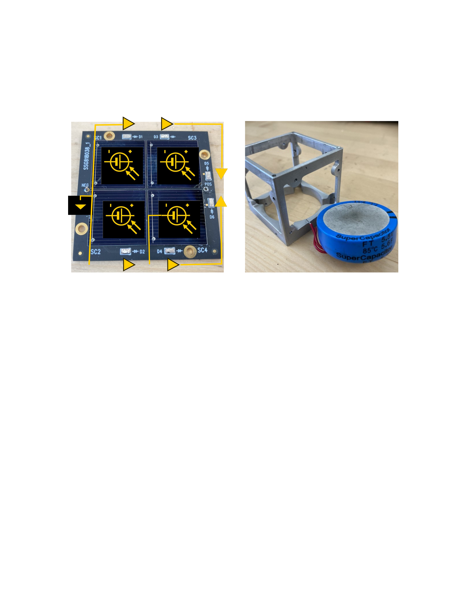
CHAPTER 7. DESIGNING AND MANUFACTURING A PICOSATELLITE 111
implementations of TAB. The satellite submodule implements TAB over its UART pins, and the simulation software
implements TAB over its serial port. Independently-designed satellite subsystems in TA1 communicate using TAB via
connected UART pins. For in-flight operation of deployed satellites, TAB commands are encoded for RF transmission
and decoded by a receiving radio. See Section 7.3.5 for a more detailed description of this use case.
Figure 7.7: Figure 7.7a shows an annotated picture of an assembled solar panel. Bypass diodes allow current to
flow while protecting against the possibility of inoperable solar cells. Figure 7.7b contains an image of the
supercapacitor used to buffer energy in TA1 next to the satellite chassis for scale.
7.3 Tartan Artibeus
Tartan Artibeus (TA1) is the first batteryless, computational pocketqube satellite; its open-source hardware and
software launched into low-Earth orbit (LEO) in January 2022. TA1 is a 1p (125 cm3) pocketqube built around the
Tartan Artibeus Bus (TAB), which connects independently-designed modules into a batteryless, computational
satellite. TA1 incorporates an electrical power supply (EPS) module that harvests solar energy into a supercapacitor,
a fault-tolerant command and data handling (C&DH) module, a radio communication module, and a configurable
computational payload module. This work presents an overview of the major components of TA1.
7.3.1 Energy Harvesting and Storage
TA1 mounts five solar panel PCBs to five of the six pocketqube faces. The sixth pocketqube face is reserved for the
baseplate and is described in Section 7.3.6. The solar panels are electrically connected to the internal electrical
power system (EPS) PCB. The power module conditions the solar panel voltages and currents and stores the
harvested energy in a 5.6 F supercapacitor. This work provides additional details for the solar panels, EPS, and
energy storage.
(a) TA1 Custom Solar Panel. (b) TA1 Supercapacitor.
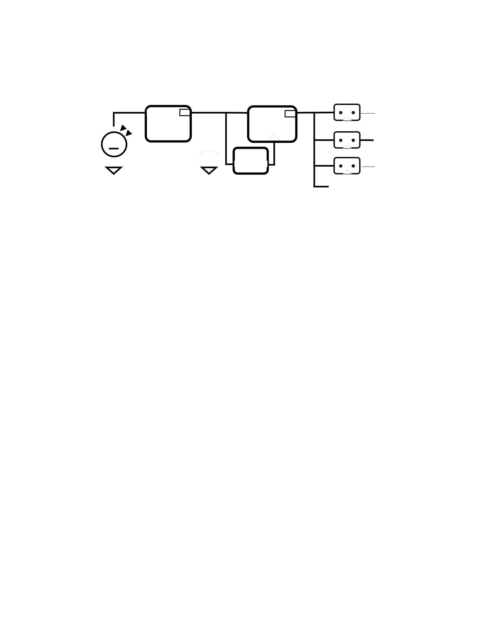
CHAPTER 7. DESIGNING AND MANUFACTURING A PICOSATELLITE 112
Solar Panels: A custom solar panel PCB covers five of the six 25 cm2 faces of the TA1 pocketqube. Each solar panel
PCB contains four square solar cells. A single solar cell measures 1.88 cm on each side.
The design first connects two cells in series to increase panel voltage, and it then connects two pairs of
Figure 7.8: TA1 Power System.
cells in parallel to increase panel current. Figure 7.7a provides a diagram of the solar panel PCB design that illustrates
the solar cell connections and the corresponding bypass diodes.
Using the standardized value for solar spectral irradiance of 1366.1 W/m2 [8] and the datasheet efficiency of
29.4% at the time of manufacture [11], each solar cell exhibits a maximum power (MP) voltage of 2.441 V and an
MP current of 58.88 mA. Thus, a single solar panel provides an MP voltage of 4.882 V and an MP current of 117.8
mA. Therefore, each solar panel provides up to 0.5751 W of power to the internal EPS PCB module. After an
extended deployment [11], MP voltage falls to 2.246 V and efficiency falls to 26.5%. Thus, MP current falls to 56.97
mA. For each solar panel, these values correspond to an MP voltage of 4.492 V and an MP current of 113.9 mA
with an overall MP of 0.5116 W.
Internal EPS PCB Module: Figure 7.8 shows a high-level schematic of the TA1 power system, which uses a dual
input-output booster design [46, 174, 148]. The input booster charges the capacitor up to 5.5 V, at which point the
voltage supervisor enables the output booster. The output booster provides a stable 3.3 V to the VDD rail and
discharges the capacitor as low as 2.0 V before the supervisor disables the output booster. The lower threshold of
2.0 V avoids inefficient charging from the input booster’s “cold-start” region.
To reduce the effort of building flexible applications for TA1, the EPS design takes on some complexity to shield
application subsystems. First, the dual booster system supports peripherals that cannot tolerate the full voltage
range experienced by the capacitor. This approach simplifies peripheral subsystem hardware development — the
developers can expect a 3.3 V input to the subsystem that is stable until the device powers down. The separate
power rails for each peripheral subsystem minimize the effort on the part of the C&DH module to disable
peripherals to save power. Features like the hardware-defined hysteresis thresholds also reduce the flight software
complexity by removing the need for software intervention [46, 156, 157]. Finally, the EPS includes onboard
measurement hardware to capture load current, harvested power, and capacitor voltage without involving off-
Input
Booster
SPV1040
Output
Booster
TPS6300
Voltage
Supervisor
TPS3806
VDD
(3.3V)
VCAP
(0-5.5V)
VSOLAR
(0-5V) COMM
EXPT
SGNS
EN
F5.6
IN OUT IN OUT
CTRL
OK
IN
Hysteresis
Loop
5.4V-2V

CHAPTER 7. DESIGNING AND MANUFACTURING A PICOSATELLITE 113
board subsystems. A four-port op-amp buffers the voltage measurements and passes the results to a 16-bit ADC
that can be accessed by any
Figure 7.9: C&DH module hardware. The C&DH MCU, the MSP430, gathers telemetry from the GNSS and IMU.
Using level shifters (LS1-3), the C&DH MCU communicates over the TAB to the attached subsystems.
subsystem via I2C. The ADC and op-amp are both powered by VDD, so when VDD is low, both are powered off.
However, the op-amp will sink current from its inputs if they are higher voltage than VDD, which would reduce the
system efficiency during charging. High impedance voltage dividers between the measured voltages and the op-
amp prevent extra current from draining.
Supercapacitor: On TA1, the EPS buffers energy in a 5.6 F supercapacitor, the FT0H565ZF (FTH) [125]. With a
total energy storage capacity of over 80 J and a maximum power output of more than 8 W, the FTH approaches the
maximum energy and power that can be stored in a 1p pocketqube form factor with a capacitor. The design also
selects the FTH for its manageable effective series resistance (ESR) over a wide temperature range. The FTH’s ESR is
expected to increase to no more than 4.2 Ω at −40 ◦C and no more than 600 mΩ at 85 ◦C. ESR limits the power a
supercapacitor can supply, so lower is better. Altitude testing confirms that the capacitor performance is not
impacted by vacuum.
7.3.2 Command and Data Handling
TA1 aims to minimize the hardware and software components responsible for persisting execution context across
power failures (see Section 7.1.2). Thus, TA1 concentrates flight control and persistency management software
onto the C&DH module. Hardware and software design choices allow C&DH to coordinate peripheral subsystems
via TAB while maintaining a large degree of isolation among these subsystems. Figure 7.9 shows the design of the
C&DH module PCB.
The C&DH module uses intentional hardware choices to provide power-failure awareness at little cost to the
peripheral subsystems. First, the C&DH MCU is an MSP430FR5994 with 256 kB of byte-addressable,
Figure 7.10: Power-failure-aware program. C&DH programs are written as a series of tasks (in green). The power-
failure-aware runtime components (in blue) correctly restart the program after a power-failure. Interrupts from the
TAB (in orange) share data with tasks through a managed buffer (center).
non-volatile FRAM (NVM) [237]. Byte-addressable NVM reduces the cost of persisting state compared to
technologies like Flash that can only be read/written at a page-granularity [44]. Second, the C&DH module uses
level shifters [235] to electrically isolate peripheral subsystems from the C&DH module. This isolation prevents

CHAPTER 7. DESIGNING AND MANUFACTURING A PICOSATELLITE 114
current from leaking across the peripheral connections when they are unpowered. Finally, the C&DH module
contains two critical sensors that provide telemetry and position data accessible by peripheral subsystems: a 9-DoF
IMU [218] and a GPS unit (with COCOM limits removed) [102]. The C&DH module hardware simplifies application
development on TA1, and the design of the programming interface is just as important.
Figure 7.10 shows an example program written with tasks (in green) that handles interrupts from the TAB (in
orange), supported by the failure-aware programming interface (keywords shown in blue) . The application
atomically walks through tasks by persistently updating the active task. If power fails in the middle of a task,
execution will resume from the start of the task on the next boot. Because TA1 is designed to support compute-
bound applications, the code does not contain any low-power wait states. Tasks execute opportunistically until
power fails.
To execute correctly, intermittent tasks must handle write-after-read (WAR) data accesses when a failed task is
re-executed [149]. Effectively, the dynamic execution gets out of sync with the persistent state and leads to
corrupted values. To prevent WAR bugs, programmers use the C&DH logging interface to write variables involved in
WAR conflicts to an undo-log [155]. On reboot, the log is replayed to restore the state of non-volatile memory to
the start of the failed task. Programmers may use a variety of tools to identify variables involved in WAR conflicts
[154, 220, 149], but they should avoid using the modified code these tools produce. The performance gap between
code produced by the production MSP430 GCC implementation [238] and LLVM-based compiler tooling [137] is
prohibitive for real systems.
The C&DH board’s non-blocking TAB implementation relies on interrupt service routines (ISRs) to process and
store packets that arrive on its UART ports. However, managing concurrent access to shared data is a challenge for
any embedded system. Intermittent execution exacerbates the problem by introducing the possibility of a power
failure during an interrupt leaving partial updates to shared state. To overcome this limitation, the C&DH software
minimizes the interface between application-defined tasks and peripheral-triggered interrupts [193], illustrated on
the right side of Figure 7.10. The C&DH software defines a restricted set of buffers that each interrupt may write
into and tasks may read from. Interrupts mark the buffers as “ready” when they may be read by tasks, at which
point tasks may extract data from the buffers and mark them as empty. Consecutive interrupts can add to the same
buffer of data, but interrupts may not read from this buffer nor any other persistent data. Instead, ISRs share data
via the buffer interface, and use static variables for state that should be retained across invocations of the ISR.
Following the task/interrupt interfacing rules prevents power failures from corrupting shared data. By providing the
underlying persistence and initialization guarantees, the C&DH board supports a wide range of application
payloads.

CHAPTER 7. DESIGNING AND MANUFACTURING A PICOSATELLITE 115
7.3.3 Computational Payload
The computational payload board consists of a custom-designed PCB around and an STM32L496RGT3
microcontroller unit (MCU). This MCU contains an ARM Cortex-M4 core: a well-documented [264],
highperformance (80 MHz) MCU with extensive open-source software support (e.g., libopencm3 [139]). The
STM32L4 series supports multiple levels of ultra low-power modes, while STM32L496 MCUs offer the maximum
amounts of integrated SRAM (320 kB) and Flash (1 MB). The STM32L496RGT3 is selected for its tolerance of
extended temperature ranges (−40 ◦C to 125 ◦C) and industrial applications rating. Additionally, the LQFP64
package supports reliable hand-soldering. Figure 7.11 illustrates the custom PCB design and an assembled board.
The ARM Cortex-M4 includes a single-precision hardware floating point unit (FPU), hardware support for digital
signal processing (DSP) instructions, hardware support for single-instruction, multiple data (SIMD) multiplication,
and multiply-accumulate (MAC) instructions [217]. As a result, the MCU core supports hardware acceleration of
machine inference. The MCU also includes an internal real-time clock (RTC) with support for operation in a low
power (320 nA) state while persisting 32 backup registers. Both
Figure 7.11: Left: The computational payload board design. Right: An assembled computational payload board.
the SRAM and Flash provide hardware error detection.
The payload PCB populates both the high-speed and low-speed crystal oscillator pins with components rated
for the extreme temperatures of space. It also populates the backup power pin with a supercapacitor containing
enough capacitance to support RTC persistence for hours. The PCB breaks out the DCMI digital camera interface
pins for future use with satellite sensors. It attaches a high-capacity (16 MB) external Flash storage chip with an
optional quad-SPI high-speed interface for storage of machine learning models and captured data. The PCB breaks
out UART pins for use with TAB.
Because space systems require accurate timekeeping for task scheduling, event timestamps, and navigation, the
TA1 computational payload board tightly integrates operation of the on-chip RTC with its CONOPS. The RTC
includes a date register and a time register. The date register stores year, month, and day by encoding the digits in
the BCD format, and the time register stores hour, minute, and second in the same format. The date and time
registers start ticking after initialization and are handled completely by hardware logic. To ensure the registers tick
at the correct frequency, the RTC clock source (either LSE, LSI, or HSE) generates a 1 Hz clock signal by prescaling its
frequency.
TA1 uses the on-chip RTC peripheral to keep time for module applications. When the computational payload
module receives power, MCU software initializes the RTC peripheral with the LSI clock source. Upon receipt of an

CHAPTER 7. DESIGNING AND MANUFACTURING A PICOSATELLITE 116
app_set_time TAB command, the MCU software initializes the date and time registers. Because the app_set_time
TAB command uses the Julian day format and the RTC registers use the Gregorian format, the MCU software
calculates a conversion. The MCU software implements a well-known procedure for this conversion [75].
7.3.4 Radio Communication
The TA1 radio communication module takes inspiration from the OpenLST [130] radio hardware and software. The
original OpenLST hardware measures 6 cm × 5 cm — too large to fit into a pocketqube form factor. In addition to
using a few difficult-to-source or deprecated components, the original OpenLST hardware makes use of three
voltage domains (5 V, 3.6 V, and 3.3 V) To simplify assembly, reduce cost, and update the design for integration with
other TA1 modules, this work heavily modifies the OpenLST hardware design. Figure 7.12 illustrates the custom
PCB design and an assembled board.
The TA1 radio communication module measures 43 mm × 43 mm so that it easily fits inside of a pocketqube.
This work replaces the deprecated power amplifier (PA) with a mass-market alternative. Following
recommendations provided by the documentation of this alternative PA, this work omits the difficult-to-source
SAW filter of the original OpenLST hardware and instead deploy a network of discrete components for filtering.
These changes eliminate all voltage domains except for 3.3 V.
To support rapid testing, the radio communication board includes two signal path options between the PA and
the antenna. Soldering one capacitor selects the “test” signal path, which terminates at a u.FL connector for use
with a COTS 50 Ω impedance antenna. Because no COTS antenna exists in a formfactor compatible with the
pocketqube standard, the radio communication board also supports a second, “flight” signal path. Soldering the
selection capacitor to a different set of pads completes this “flight” signal path, which terminates at a solder point
preceded by pads for an L-matching network. TA1 uses a custom-designed, nitinol antenna. After matching the
antenna length to the half-wavelength of the center operating frequency, the appropriate passive components
match the antenna impedance to the signal path.
Despite significant hardware changes, the OpenLST software remains largely unchanged. As in OpenLST, the TA1
radio leverages the CC1110 RF MCU. This work modifies GPIO software logic to support an alternative RF switch,
and it modifies frequency specification variables to reflect the 401.82 MHz at which the board is licensed to
operate. TAB makes integration of pre-existing modules seamless and straightforward.
7.3.5 Radio Link Analysis
Under a bent-pipe CONOPS, RF communication plays a key role in the satellite mission. Even under OEC, RF
communication occupies an indelible position in satellite operations: delivering processed data to the ground
segment. Therefore, the RF CONOPS requires sufficient link budget and appropriate error correction in the packet

CHAPTER 7. DESIGNING AND MANUFACTURING A PICOSATELLITE 117
design. Error correction plays a particularly important role in satellite missions due to artifacts inherent to long
range, high velocity satellite communications such as the doppler effect.
Figure 7.12: Left: The radio communication board design. Right: An image of an assembled communication board.
These effects are less prevalent in terrestrial communication scenarios.
Because the small form factor and associated power constraints of TA1 prevent boosting transmit power
arbitrarily high (within the FCC regulations), this work uses a modified version of OpenLST [130] based on the
popular CC1110 [85] radio transceiver platform for low power operation of the RF subsystem. This work describes
the packet structure, link budget, and the ground station demodulation and decoding pipeline of TA1.
Packet Structure and Transmit Pipeline: Figure 7.13(a) shows the packet structure in the radio communication
module, which is based on the CC1110 pipeline. It contains a 4 byte preamble consisting of an alternating sequence
of 1010 . . . bits and a 2 byte sync word that can be set by the user. The preamble sequence helps in packet
detection and the sync word aids in byte-level synchronization as well differentiating packets from other sources
transmitting using the same platform in the absence of the address field. This sequence is followed by the length
and payload fields. The former indicates the length in bytes of the payload. The maximum payload length is 255
bytes. Finally, a 16-bit CRC concludes the payload to ensure bit error detection and correction.
After packet creation, the bits undergo appropriate coding and modulation before being transmitted over the
air. Figure 7.13(b) describes the bits-to-symbol encoding and modulation pipeline. Bits are first whitened using a 9-
bit pseudorandom sequence [234] defined by the generator polynomial x9 + x5 + x0. Data whitening ensures bit
randomization, which protects against DC bias introduced in the transmit signal due to a burst of continuous 0s or
1s. The whitened data is then convolutionally encoded [191] using a half rate encoder defined by the generator
polynomials g1 : x3 + x1 + x0 and g2 : x3 + x2 + x1 + x0, respectively, to ensure robustness to channel-induced errors.
Post encoding, the data is interleaved using a 4 × 4 interleaver to ensure robustness to burst errors that can be
introduced due to channel fading. The interleaved bits are encoded in 2-FSK modulation and transmitted over the
air using the baud rate of approximately 7.5 Kbaud. Both the modulation format and baud rate are user-specific
fields that can be modified based on need. It should be noted that the preamble and sync word fields do not
undergo the whitening, encoding, and interleaving transformations, while the rest of the fields in the packet do.
RF Characteristics and Link Budget: The 2-FSK modulation essentially encodes bits 0 and 1 using two
frequencies, −f/2 and f/2 respectively, separated by a two-sided bandwidth of f (approximately 7.5 kHz in TA1). This
fact can be seen as two prominent peaks in the frequency spectrum of the received signal. The link budget analysis
can be broken down as follows:
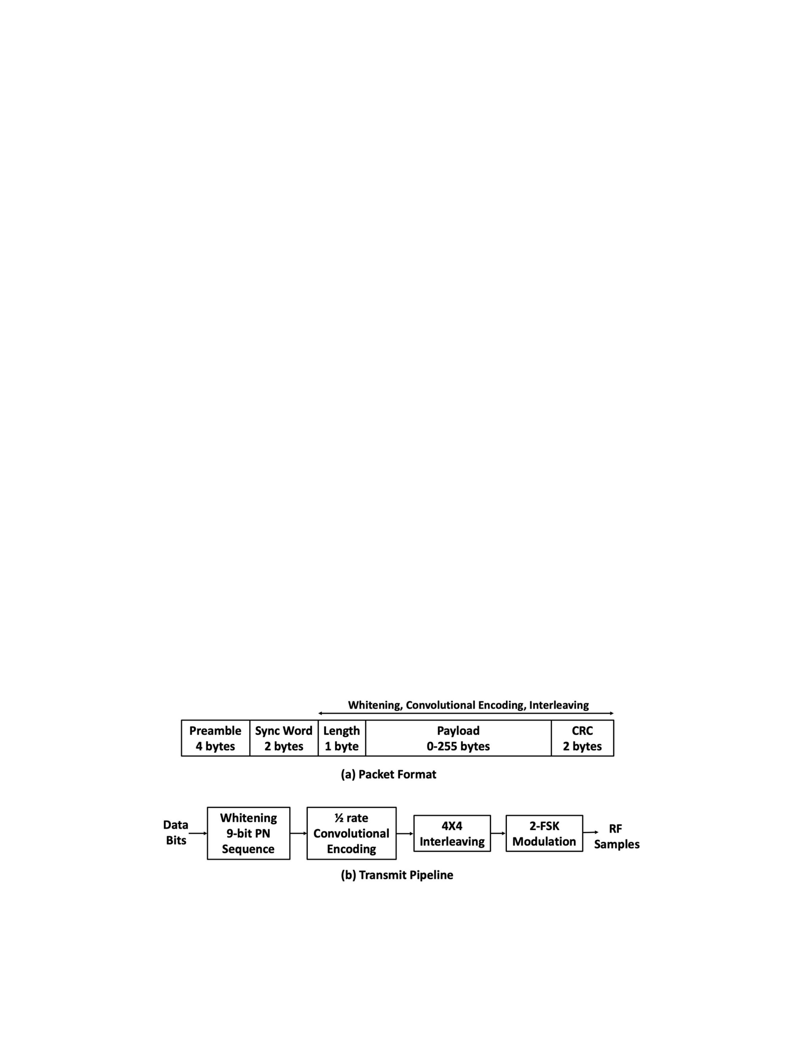
CHAPTER 7. DESIGNING AND MANUFACTURING A PICOSATELLITE 118
1. Transmitter: The RF signal is transmitted from the satellite using a maximum transmit power of 1 W (30
dBm). This transmit power can be throttled based on the power availability on the satellite.
Assuming unity gain antenna at the satellite, these factors provide an Equivalent Isolated Radiated Power
(EIRP) of 30 dBm.
2. Path loss: The orbital altitude of 500 km along with transmit frequency of 401.82 MHz results in a free space
path loss of 138.5 dB. Note that the actual distance can vary, depending on the exact relative distance
between the satellite and the ground station, which varies as the satellite moves in its orbit.
3. Receiver: Any SDR-based ground station would receive the signal at a bandwidth slightly higher than the
transmitter to ensure decent oversampling factor that can be used to average out noise. Receiving the
satellite signal at a 5× oversampling results in a noise floor of −128 dBm. Accounting for a 6 dB noise factor
introduced by any hardware, it is safe to assume an effective receiver sensitivity of −116 dBm. In order to
ensure a good signal-to-noise-ratio (SNR) of 10 dB for 2FSK modulation, any received signal with power over
−106 dBm should be decodeable. Removing path loss from EIRP and accounting for a 10 dB antenna gain at
the ground station, the received signal power at the ground station comes out to be −98.8 dBm, which in
turn results in a SNR of approximately 18 dB. This SNR is more than sufficient to ensure successful decoding.
While the numbers used in this analysis are typical values, in case of higher path loss or higher bandwidth
(noise floor) or lower transmit power, a higher gain antenna with a low noise amplifier can be used at the
ground station to ensure sufficient SNR for successful decoding.
Demodulation and Decoding Pipeline: While on-chip decoders use the exact same parameters like bandwidth,
gain, etc. for demodulation and decoding, employing an SDR-based ground station provides more flexibility to
record at higher gain and debug in low SNR scenarios. This work creates a demodula-
Figure 7.13: TA1 radio communication module (a) packet format, and (b) transmit pipeline

CHAPTER 7. DESIGNING AND MANUFACTURING A PICOSATELLITE 119
tion and decoder script to process the received signal from any SDR operating at any acceptable receiver
bandwidth (> 2× the transmit bandwidth). Using a higher bandwidth at the SDR provides a higher oversampling
factor that gives two benefits: a larger number of RF samples to yield a higher preamble and syncword detection
gain, and a larger number of samples to disambiguate the FSK symbol frequency while demodulation. Packet
detection and demodulation benefits from these two aspects. This work first detects the packet using a large
number RF samples to improve the chance of detection and then demodulate to bits. In comparison, an on-chip
system first demodulates to bits and then detects the packet using much fewer bits thus reducing the chance of
detection. Upon demodulation to bits, this work reverses the steps described in Figure 7.13(b) to recover the
transmitted message.
7.3.6 Baseplate, Chassis, and Mechanics
The TA1 stacked-PCB design inside the pocketqube form factor eliminates many mechanical questions encountered
by cubesats. For TA1, the mechanical design effort concentrates in the chassis, the sliding baseplate required by the
pocketqube standard, and compliance testing required by the launch provider. Figure 7.14a shows the 115 g
aluminum chassis, co-designed with the solar panel PCBs also pictured. The in-house mechanical design group
TechSpark at Carnegie Mellon University modeled and manufactured the chassis. The chassis connects to the
baseplate using four standard M2 screws, and custom aluminum standoffs affix the stack of modules to the
baseplate to provide an electrical chassis ground to the modules.
The baseplate is a critical component of the TA1 design that resolves mechanical, electrical and compliance
requirements. Figure 7.14b shows a labeled image of the baseplate. In addition to the connection to the chassis,
the baseplate electrically connects to all of the pins used by TAB to communicate between modules and exposes
them for testing, debugging, and pocketqube standard compliance. In the pocketqube standard, the baseplate is
primarily defined as the interface to the pocketqube launcher. In
(a) TA1 chassis. (b) TA1 baseplate.
Figure 7.14: TA1 Mechanical Components. The TA1 chassis (left) and baseplate (right) comply with the pocketqube
standard and electrically attach key components.
addition to adhering to the required dimensions, the baseplate must provide mechanical “kill switches” that keep
the satellite powered off until deployment. Leveraging the baseplate module connections, the kill switches short
the supercapacitor voltage to chassis ground when the satellite is inside the launcher, depressing the switches.
Connecting the supercapacitor to ground over a low resistance (100 Ω) prevents any errant harvested energy from
accruing in the supercapacitor before launch. Beyond its required functionality, TA1 utilizes the baseplate to

CHAPTER 7. DESIGNING AND MANUFACTURING A PICOSATELLITE 120
mechanically secure the GNSS antenna [233](Figure 7.14b, B), provide a convenient connection to the solar panels
(Figure 7.14b, C), and hold the antenna release mechanism (Figure 7.14b, D). The radio module nitinol antenna is
secured before launch by wrapping it against the baseplate and tying it to a nichrome wire [166] with fishing line
[20]. On first boot, the C&DH module activates a high power transistor that shorts the supercapacitor to ground
over the nichrome wire. The resulting current flow causes the nichrome wire to heat up and melt away the
monofilament fishing line, releasing the antenna.
Once the pocketqube standards are met, compliance with the launch provider must be satisfied. To
mechanically test TA1, this work carries out qualification level testing on the final TA1 flight unit for random
vibration and sine burst testing [72]. No damage was incurred on TA1 throughout these tests, and the unit
functioned as expected afterwards. Additionally, TA1 must meet outgassing requirements set by the launch
provider [216]. This work applies a conformal coating to both sides of each module and the baseplate to prevent
substantial outgassing from any of the electrical components. Interestingly, the conformal coating resulted in an
unspecified conflict with the pocketqube standard. The coating increased the friction between the edge of the TA1
baseplate and the pocketqube launcher rail [186] and prevented TA1 from sliding freely. To launch, the coating had
to be removed along the 2 mm overlap between the baseplate and the rail. Future revisions to the pocketqube
standard should specify the acceptable coefficient of friction between the baseplate and the launcher rail.
7.4 TAB Reference Applications
To evaluate the TA1 implementation of TAB, this work presents three reference applications. These applications
illustrate the concept of operations (CONOPS) of TA1. Each application makes use of TAB. The first application,
“ping,” exercises the TA1 radio module. The second application, “data,” exercises both the radio module and the
C&DH module. TAB messages are received by the radio module, parsed, and forwarded to the C&DH module
destination. The third application, “cote,” exercises the radio module, the C&DH module, and the computational
payload module. TAB messages are received by the radio module, parsed, and forwarded to the C&DH module for
delivery to the computational payload module.
7.4.1 Application 1: Ping
The “ping” application consists of a single command, which generates a single reply. A ground station emits a
common_ack via RF (see Section 7.3.5) for reception by TA1. To be accepted, the hardware ID of the common_ack
must match the hardware ID of TA1. All TA1 modules have been programmed with this
hardware ID.

CHAPTER 7. DESIGNING AND MANUFACTURING A PICOSATELLITE 121
This application aims to elicit a reply from the radio module. Therefore, the common_ack destination ID
contains the radio module ID as the lower nibble. To indicate that the reply should be transmitted via RF, the upper
nibble contains the ground station ID. Upon reception, the radio module generates a common_ack response. The
upper and lower nibbles of reply destination ID are swapped as described in
Section 7.2.2.
7.4.2 Application 2: Data
The “data” application demonstrates the ability of TAB to support communication between modules. This
application requests telemetry stored on the C&DH module. Every minute, TA1 collects data from the IMU on the
C&DH board as well as the time, date, position, and status information from the GNSS and power introspection
information from the ADC on the EPS. These data are pushed onto a stack until a telemetry request command
arrives. In response, the C&DH module pops the most recent telemetry for
reply.
7.4.3 Application 3: cote
The “cote” application consists of a single command that ultimately results in a single reply. However, this
application exercises three TA1 modules: the radio module, the C&DH module, and the computational payload
module. This “cote” application implements a limited version of the open-source cote simulator for computational
nanosatellites [53]. Specifically, this work ports the cote implementation of SGP4 [99] from C++ to C for execution
on the computational payload MCU. Given a TLE via a common_ascii
command, the payload board leverages the MCU RTC to calculate the current position of the satellite and generate a
message containing these coordinates. See Figure 7.6 for a diagram of this application.
7.5 Additional TAB Applications
TAB supports over-the-air upload of new software applications after deployment to orbit. Post-deployment updates
make TA1 a flexible orbital edge computing research platform. This upload mechanism has been demonstrated in
the lab, as well as the ability to time-multiplex several programs on a single payload board. This feature provides a
first step toward dynamic multitenancy and new, flexible “software-defined nanosatellite constellations.”
The application upload mechanism delivers new programs to the satellite via RF; upon delivery, these programs
are stored for execution. This implementation uses Intel’s line-oriented HEX format, which includes a per-line start
code, byte count, address, record type, data, and checksum. The start code specifies the record type and, if the line

CHAPTER 7. DESIGNING AND MANUFACTURING A PICOSATELLITE 122
start code indicates a data record, the TA1 ground support software [58] parses data from that line for
transmission. After collecting all data lines, the data are split into 128-byte “chunks” for use in the
bootloader_write_page TAB command. These commands are sent
to the computational payload board, where the program data are written into storage.
Simultaneous deployment of multiple programs requires a more general TAB command than the backwards-
compatible bootloader_write_page command. Specifically, in order to make use of the entire address range of the
program storage, TAB introduces the bootloader_write_page_addr32 command. This new, more general command
writes the 128 byte TAB payload starting at the address in memory specified in the command. This new, more
general TAB command is exercised in the lab by demonstrating a computational payload board with three user
programs. Each user program executes in response to a TAB bootloader_jump command.
7.6 Summary
This work presents Tartan Artibeus, an open source hardware [55] and software [56] 1p pocketqube satellite
launched into LEO in January 2022. Built around the Tartan Artibeus Bus (TAB), TA1 integrates independently-
designed modules into a batteryless, computational satellite. TAB positions TA1 as a platform for computational
nanosatellite research by supporting (i) interaction between software simulation environments and research
hardware (hardware-in-the-loop); (ii) integration between independentlydesigned satellite subsystems; and (iii) in-
flight operation of deployed satellites.
This work provides in-depth descriptions of the satellite mechanics, PCB hardware design, software, system
CONOPS, and radio communication to serve as a blueprint for other organizations working in computational space
systems. Detailed bills of material (BOMs), MCU software, communication protocol and CONOPS documentation,
and ground station software are available publicly. TA1 serves as a lowcost, compliance-tested research platform
and satellite for LEO operations.

Chapter 8
Conclusion
Emerging satellite platforms require software, hardware, and system support to address communication,
computation, and energy constraints. Orbital edge computing co-locates state-of-the-art, embedded processing
systems with sensors in nanosatellites to intelligently discard low-value data before downlink [52]. Computational
nanosatellite pipelines distribute data collection and processing across devices to address processing time and
energy availability limitations [53]. Software-based scheduling, application emulation, and context-aware
application specialization further improve satellite utilization [51]. These hardware and system contributions are
evaluated with a custom, open source, full-system simulator for astrodynamics, energy, data, computation, and
communication [53]. A custom, open source hardware satellite provides a platform for evaluation of these
contributions in orbit [57]. The opportunities of orbital edge computing [148] enable new, constellation-level
system designs [37] addressing the challenges experienced by existing operating strategies for satellites.
Chapter 3 introduces the concept of data quality constraints unique to Earth-observation satellites. Altitude,
camera focal length, and pixel sensor size determine satellite image feature sizes. Higher altitudes make features
smaller, while longer focal lengths and smaller pixel sensor sizes make features larger. The accuracy of
convolutional neural networks used to analyze these images varies significantly according to these feature sizes.
Orbital edge computing systems must be aware of these constraints to support useful computation. This chapter
describes power and software optimizations for the orbital edge and uses formation flying to support device-
parallel computation in space.
Chapter 4 leverages the observations quantified in Chapter 3 and introduces additional techniques to trade
execution time and accuracy at the orbital edge. Data-filtering applications directly deployed to the orbital edge
experience a computational bottleneck on existing and near-future satellite hardware. The sensor and orbit
characteristics of a target satellite impose a processing deadline. By adjusting execution
131
CHAPTER 8. CONCLUSION 132
time, sometimes at the expense of accuracy, the data value density of the saturated downlink increases. Methods
to transform a reference application and increase data value density include frame tiling, context specialization,

and context-based processing elision. Intelligently filtering low-value data and prioritizing high-value data for
transmit via the saturated downlink increases the data value density between 89 and 97 percent.
Another technique — computational nanosatellite pipelines, or CNPs — is introduced in Chapter 5 as a means
for addressing the computational bottleneck. By distributing work across a constellation, a collection of
nanosatellites processes observations faster than the ground track frame rate and achieves full ground track
coverage. This approach is uniquely possible with the low, individual cost of nanosatellites and the expanded
availability of launch opportunities. By launching and replacing nanosatellites in a constellation early and often,
sufficient computational capability exists across the system in aggregate. These OEC architectures can reduce
ground infrastructure over 24× compared to a bent-pipe architecture, and CNPs can reduce system edge
processing latency over 617×.
Chapter 6 introduces Horizon, a system to schedule satellite subsystem operations within energy storage and
data storage constraints. Horizon considers energy and data buffer size constraints and their interaction with the
previously-identified constraints of communication and computation. Efficient utilization of emerging LEO satellite
constellations requires that these constraints be identified, understood, and addressed. Each satellite subsystem —
e.g., sensors, ADACS, onboard computer, and radio — operates in one of many possible states. The schedule of
these subsystem states has a dramatic impact on end-to-end system performance. Horizon supports a more than
81% increase in processed data downlinked per orbit period and, in the case of energy-constrained systems, a more
than 36% increase in unprocessed data downlinked per orbit period.
Finally, Chapter 7 presents Tartan Artibeus: an open-source hardware and software reference implementation
of a flight-ready picosatellite for in-situ OEC evaluation. The Tartan Artibeus Bus (TAB) provides a communication
framework for easy integration of flight hardware with both software simulation environments and new hardware
research modules (e.g. experimental payloads). TAB also supports command and control of the satellite in orbit.
Flight software includes three reference applications that exercise TAB and provide a model for in-orbit OEC
research. Deploying and operating satellites in space is an important aspect of orbital edge computing research
that reveals system performance bottlenecks and validates modeling and simulation results.
This work introduces orbital edge computing for computational nanosatellites. Historically, satellites operate as
dumb, remote-controlled sensors. This concept of operations worked well for nearly 70 years when each satellite
was an expensive, exquisite, specialized, one-of-a-kind device that must minimize risk CHAPTER 8. CONCLUSION
in response to high cost. As low-Earth orbit becomes more accessible, this manual operating strategy no longer
scales. To maximize the utility of space systems in a proliferated low-Earth orbit, each device must autonomously
react to sensor data at the space edge. Orbital edge computing provides software, hardware, and system support
to filter observations in space with constraints on data quality, communication, computation, and energy. Over the

next five to ten years, low-Earth orbit is expected to experience an elbow event in satellite count; the rate at which
new satellites deploy to LEO will be dramatically higher than the relatively steady rate of new deployments during
the previous 65 years. For the first time, active satellite count could experience a 3× growth over just a few years.
As a result, orbital edge computing systems research has a bright future across many domains, including computer
architecture, robotics, aerospace, cyber-physical systems (CPS), computer networks, and many other fields.

