



A Model-Based Framework for Analyzing Cloud Service Provider Trustworthiness
and Predicting Cloud Service Level Agreement Performance
Chapter 1. Introduction
A 2017 cloud survey from Skyhigh Networks and Cloud Security Alliance (Skyhigh
2017) identified the following key drivers for moving applications to cloud infrastructure
(i.e. Infrastructure-as-a-Service providing subscription based processors, storage,
network, software): increased security of cloud platforms, scalability based on workload,
preference for operating expense vs capital, and lower costs. Despite these drivers, key
challenges exist. A 2017 cloud survey from Rightscale (RightScale 2017a) identified
challenges that included complexity and lack of expertise, security, ability to manage
cloud spend, governance and ability to manage multiple cloud services. Clearly, there is
overlap between the drivers and challenges, with lots of potential for financial risk and
missed service level expectations.
1.1 Problem Description
As of January 2017, 95% of companies (RightScale 2017a) are dependent on
Infrastructure-as-a-Service (IaaS) cloud service providers, and as cloud computing usage
increases (400% 2013-2020 (Mason, Kelsey and Krieger 2016)), impact to service levels
and financial risk from data center outages increase (81% 2010-2016 (Ponemon 2017)).
For example, the cost of data center outages in 2015 for Fortune 1000 companies was
between $1.25 and $2.5 billion (Ponemon 2017). Of the data center outages between 2010
and 2016, 22% were caused by security (Ponemon 2017). Furthermore, data breaches
1

were up 40% in 2016 (IDTC 2016). With the increased demand and dependency on cloud
computing, risk to expected service levels (e.g. availability, reliability, performance,
security), potential for financial impact, and level of trustworthiness of cloud service
providers (CSPs) are all important areas requiring attention. For this Praxis and based on
previous work reviewed throughout the Literature Review in Chapter 2, CSP
trustworthiness is defined in terms of historical quality of service (QoS), current
capabilities and transparency, and future performance. For historical QoS, did the CSP
deliver what they said they would deliver? Did they meet cloud service customer (CSC)
expectations? How comprehensive and transparent are the CSP’s delivery and security
capabilities (e.g. what is their level of CSA CCM compliance)? With respect to future
performance, does the CSP have the required capabilities to meet future CSC’s service
level requirements as represented by cloud SLAs?
1.2 Solution Approach
To address the need, cloud computing service level agreements (SLAs) and a model
for assessing, predicting and governing performance of cloud services and service levels
are required to mitigate cloud computing service level risks and impact (e.g. availability,
reliability, performance, security, financial). Research objectives related to this proposed
solution are focused on analyzing CSPs and cloud computing services, and predicting
cloud SLA performance. Industry standards and evolving research related to cloud
computing SLAs (EC 2014, Hunnebeck et al. 2011, ISO/IEC 2016, NIST 2015, Hogben,
Giles and Dekker 2012) and CSP trustworthiness (Ghosh, Ghosh and Das 2015, Taha et
al. 2014) will be leveraged. A predictive model (using Linear Regression Analysis) was
built for calculating SLA performance based on industry standardized cloud SLAs, CSP
cloud service performance, CSP trustworthiness and other cloud computing
2

characteristics. With the focus on cloud computing service levels, the literature review is
organized around the lifecycle of cloud computing service level agreements. The lifecycle
is comprised of four phases: Cloud Computing SLA specification, Cloud Service Provider
Trust Models, Cloud Computing SLA monitoring, and Cloud
Computing SLA enforcement. Details are provided in the Literature Review chapter.
The expected outcome from the methodologies is the creation of a model that predicts
cloud computing SLA availability. The methodologies used included Graph Theory to
analyze and model cloud SLAs, Analytic Hierarchy Process to calculate CSP
trustworthiness, and Linear Regression Analysis to build the predictive model based on
multiple variables, including output from the other methodologies. The research
methodologies, hypothesis and expected outcomes are reviewed further in Chapter 3
Methodology as well as the flow of data and dependencies between the methodologies.
1.3 Contribution
Due to the described cloud computing challenges, risks and impacts, cloud service
customers (CSCs) may be unable to trust cloud service providers (CSP). Trust needs to
be based on more than CSP’s claims. With security being one of the most important
factors that can influence trust between the CSPs and CSCs, the Cloud Security Alliance
(CSA) designed the Cloud Controls Matrix (CCM) (CSA CCM 2017) and Consensus
Assessments Initiative Questionnaire (CAIQ) (CSA CAIQ 2017) to assist CSCs when
assessing overall security capabilities of the CSP. While security remains a priority and
rightly so, measuring and establishing CSP trust should consider criteria based on a
comprehensive quantitative and qualitative assessment of CSP capabilities, CSC service
level requirements, and CSP cloud service historical performance. An appropriate
3

methodology and model is required to assess the CSP with respect to the broader set of
trust criteria, including evaluating cloud computing service level agreements (SLAs)
between the CSC and CSP, and predicting cloud SLA performance (e.g. cloud service
Availability). The research contribution with respect to the proposed methodology and
model is structured into a cloud computing SLA lifecycle, with four phases.
•Cloud Computing SLA specifications, their importance, benefits, standards and
frameworks.
•Cloud Computing trust models based on CSP capabilities, performance,
transparency and trustworthiness.
•Cloud Computing monitoring and CSP trust levels based on quality of service
(QoS) and SLAs.
•Cloud Computing SLA enforcement through proactive QoS management and
autonomic computing.
1.3.1 Cloud SLA specifications - benefits, standards and frameworks
While there has been a significant amount of work related to cloud SLA standards
(e.g. ITSMF ITIL, ISO/IEC, NIST, EC) (Hunnebeck 2011, ISO/IEC 2016, NIST 2015,
EC 2014), adoption lags and CSPs continue to offer proprietary and diverse SLAs. The
industry SLA standards (ISO/IEC 2016, NIST 2015, EC 2014), industry cloud security
controls (CSA CCM 2017), cloud security audits and SLAs for CSPs (e.g. Amazon,
Google, Microsoft) (STAR AWS 2017, STAR Google 2017, STAR Microsoft 2017, SLA
AWS 2017, SLA Google 2017, SLA Microsoft 2017) were analyzed with overlaps and
gaps highlighted. A standard cloud SLA structure was confirmed and leveraged during the
CSP trust modeling.
4

1.3.2 Cloud trust models based on CSP capabilities and transparency
Research related to CSP trustworthiness and trust models has received significant
attention and has influenced CSP assessment and selection. The CSP trust model research
was organized around fuzzy logic evaluation (Wu and Zhou 2016, Mitchell, Rizvi and
Ryoo 2015, Qu, Wang and Orgun 2013, Supriya, Sangeeta and Patra 2015), security
(Kanpariyasoontorn and Senivongse 2017, Luna, Langenberg and Suri 2012, Taha et al.
2014, Luna et al. 2015, Almanea 2014, Roy, Sarker and Hashem 2015), quality of service
(QoS), and SLAs (Naseer, Jabbar and Zafar 2014, Ghosh, Ghosh and Das 2015, Ristov
and Gusey 2015, Chakraborty, Sudip and Roy 2012, Ruan et al. 2016). CSP cloud SLAs
reflect a CSP’s service level obligations and capabilities (including security).
Consequently, the CSPs obligations and capabilities influence cloud service performance
and SLA compliance. The standard cloud SLA structure from phase one was assessed for
each CSP (i.e. Amazon, Google, Microsoft) and then factored into their trustworthiness
comparison and calculation (i.e. CSP trust level). The CSP trust level was then applied by
the third phase and integrated with CSP historical cloud service performance and cloud
service characteristics to predict cloud SLA performance (e.g. cloud service Availability).
1.3.3 Cloud monitoring and trust levels based on QoS and SLAs
Research related to monitoring and measuring information technology (IT) resources,
their quality of service (QoS), and relationships with cloud services has received much
attention over the years (EC 2014, Natu et al. 2016, Ghosh, Ghosh and Das 2015, Taha et
al. 2014, Emeakaroha et al. 2010, DMTF 2015). The contribution to this research
emphasized the association of measuring and monitoring the performance of cloud
service IT resources with CSP trustworthiness and cloud SLA performance. The analysis
5

and calculation of CSP trustworthiness (i.e. CSP trust level) was extended beyond
security, and factored in cloud service level objectives and cloud qualitative objectives of
the SLA (EC 2014, ISO/IEC 2016). The research contribution then constructed a model
for predicting cloud SLA performance (i.e. cloud service Availability), and applied the
association (i.e. CSP trustworthiness integrated with CSP cloud service characteristics,
cloud service and SLA performance) towards the calculation and prediction.
1.3.4 Cloud SLA enforcement through proactive QoS and autonomic computing
Cloud orchestration, containers and autonomic self-managing clouds have been active
research areas (Linthicum 2016, Diaz-Montes et al. 2016, DMTF 2015, Ferry et al. 2013).
These areas are essential for driving governance and automation of cloud services and
related IT resources. Ultimately, driving the governance and automation based on SLAs is
a key objective. With a model for predicting cloud SLA performance, the necessary CSP
and cloud service changes can be made to proactively increase CSP trustworthiness and
cloud service performance, thereby improving cloud SLA performance and driving SLA
compliance.
1.4 Research Contribution Objectives, Questions and Hypothesis
To drive the research contributions across the SLA lifecycle phases, the following
objectives for the research were established.
•To assess industry related cloud SLA standards and structures.
•To define a CSP trustworthiness framework based on analysis of CSP compliance
with the cloud SLA standards and security frameworks and establish CSP trust
levels.
6

•To develop a model for predicting cloud SLA performance (i.e. cloud service
Availability) based on a standard cloud SLA structure, CSP trustworthiness, and
historical CSP cloud service performance and characteristics.
•To evaluate and validate the predictive model, and assess the observations and
predictions related to predicting cloud SLA performance (i.e. cloud service
Availability).
In support of the objectives, the following questions and actions were considered.
•What value do the SLAs offered to CSCs by CSPs provide?
•What gaps exist between SLAs provided by CSPs compared to emerging industry
cloud SLA standards?
•As SLA’s are reviewed, CSPs trustworthiness was assessed in terms of historical
CSP cloud service performance, and breadth and depth of SLA structure including
security coverage as vetted against CSA’s CCM (CSA CCM 2017) and CAIQ
(CSA CAIQ 2017).
•To analyze historical CSP (i.e. Amazon, Google, Microsoft) cloud services and
SLA performance, Gartner’s Technology Planner Cloud Module (renamed Cloud
Decisions) was utilized (Gartner 2017).
•When evaluating CSP trustworthiness and historical cloud service performance,
consider whether the CSP delivered what they said they would deliver … did they
meet service level expectations?
•When predicting cloud SLA performance, consider whether the CSP and cloud
services have the required capabilities to meet future service level expectations?
7

To assess the research contributions, the following hypothesis was proposed. The
expected results related to the hypothesis were based on the composite outcomes of the
methodologies (i.e. Graph Theory, Analytic Hierarchy Process, Linear Regression
Analysis). The hypothesis proposed and tested was:
Predicting SLA-based cloud service availability has greater accuracy when
calculated with more criteria than just historical cloud service downtime (e.g. CSP
trustworthiness; global cloud service locations, resource capacity and performance). The
primary question to be answered: Does predicting cloud computing SLA performance
have a greater accuracy when calculated with historical SLA performance, cloud service
performance, and CSP trustworthiness, rather than just historical cloud service downtime?
1.5 Organization of Chapters
This praxis is organized into five chapters and appendices. Chapter 1 Introduction -
introduces drivers and key challenges for moving applications to the cloud. The
percentage of organizations adopting the cloud and growth is reviewed along with risks
and impact. The proposed solution, research objectives and related methodologies are
described plus industry research associated with the solution. The research approach and
contributions are reviewed; and research questions, hypothesis, and methodologies used
to produce the results are introduced.
Chapter 2 Literature Review - provides background information concerning previous
and current research related to the area of cloud computing SLAs, CSP trustworthiness
models, monitoring cloud services and SLA performance, and predictive and proactive
management and mitigation of risk and impact.
Chapter 3 Methodology – reviews the research methodologies and step by step
statistical approaches for the research which include Graph Theory, Analytic Hierarchy
8

Process, and Linear Regression Analysis. The research data is analyzed and relationships are
investigated between cloud SLAs and security frameworks, CSP trustworthiness models, cloud
service performance and CSP cloud service characteristics.
Chapter 4 Results – presents the statistical results from each of the methodologies
(Graph Theory, Analytic Hierarchy Process, Linear Regression Analysis). The research
findings are organized based on the methodology map, which reviews the integration of
the methodologies and their flow to the predictive model.
Chapter 5 Conclusion – summarizes the findings and presents the conclusions of the
research. Applications for the research and how it could be used are reviewed. The
chapter also discusses limitations and related opportunities for future research.
Lastly, the Appendices present a number of tables referenced by the Chapters.
Appendix A presents the entire dataset used for the research (Gartner 2017). The dataset
is based on real observed CSP cloud compute service data as well as CSP cloud service
location and service region characteristics. Appendix B presents work contributed by
standards organizations ISO/IEC, ENISA and EC towards standardized cloud SLAs
(ISO/IEC 2016, Hogben, Giles and Dekker 2012, EC 2014). Appendix C presents
security related frameworks, controls and requirements from the Cloud Security Alliance.
The frameworks include the Cloud Controls Matrix ( CCM) and Consensus Assessment
Initiatives Questionnaire (CAIQ) (CSA CCM 2017, CSA CAIQ 2017). Appendix D
presents the cloud SLA Content Area to CCM Control Domain mappings and CIAQ
compliance for each CSP (CSA CAIQ 2017, STAR AWS 2017, STAR Google 2017,
STAR Microsoft 2017). Appendix E reviews the cloud SLAs offered by CSPs Amazon,
Google and Microsoft (SLA AWS 2017, SLA Google 2017, SLA Microsoft 2017).
9

Appendix F summarizes Goodness of Fit measures for both simple and multiple linear
regression models that were calculated and analyzed using R functions. Appendix G
represents CSP Comparison Matrices for SLA Content Areas utilized by AHP. Appendix
H represents CSP Priority Vectors for SLA Content Areas related to Appendix G and
utilized by AHP processing. Appendix I presents Degree Centrality details for all graphs.
10

Chapter 2. Literature Review
Over the past two decades in the Information Technology (IT) industry, a significant
amount of important work occurred related to managing service levels and service level
requirements, e.g. IT Service Management Forum Information Technology Infrastructure
Library (Hunnebeck 2011). Related to this work, service level agreements (SLAs) have
been established as written agreements between service providers and IT customers.
SLAs define key service targets and responsibilities, and serve as a basis for managing
the relationship and establishing trust with the service provider. Within the cloud
computing community, service level management and SLAs are also increasingly being
adopted. Over the past few years, the European Commission has established the industry
group (Cloud Select Industry Group – Subgroup on Service Level Agreement: C-
SIGSLA), to provide a set of SLA standardization guidelines (EC 2014) for cloud service
providers (CSPs) and cloud service customers (CSCs). There is also work at the
international level with ISO/IEC 19086 (ISO/IEC 2016) from the ISO Cloud Computing
Working Group. With the momentum and need around managing cloud computing
service levels, the literature review is organized around four phases of the lifecycle of
cloud computing service level agreements.
The first phase in the lifecycle focuses on Cloud Computing SLA specifications, their
importance, benefits, standards and frameworks. A significant amount of work has been
done by standards organizations (e.g. ITSMF ITIL, ISO/IEC, NIST, EC) (Hunnebeck
2011, ISO/IEC 2016, NIST 2015, EC 2014) related to defining standardized cloud SLAs.
However, the work is not complete. CSP SLAs are diverse and gaps include adoption and standard
methods for verifying compliance along with linking SLA compliance to predictive and proactive
automation.
11

The next phase of the lifecycle is Cloud Computing trust models based on CSP
capabilities (e.g. security), transparency and trustworthiness. Over the past few years,
CSP trust models and CSP trustworthiness specifically related to cloud security have
received significant attention. However, gaps exist with respect to considering both
historical service level performance and other service level capabilities (vs just security)
that can influence future performance. Questions to address when assessing CSP
trustworthiness for historical performance include: historically, did the CSP deliver what
they said they would deliver…did they meet service level expectations; and regarding
future performance, does the CSP have the required capability to deliver against future
service level expectations (not just security but all aspects of the SLA)? Existing trust
model and trustworthiness research related to CSP assessment, evaluation and selection is
organized into the following three groups.
•CSP evaluation and selection with fuzzy logic based trust models.
•CSP assessment and trustworthiness based on security capabilities and Cloud
Security Alliance (CSA) Cloud Controls Matrix (CCM).
•CSP selection and trustworthiness based on SLAs and QoS requirements.
The third phase of the lifecycle is Cloud Computing monitoring and CSP trust levels
based on quality of service (QoS) and SLAs. Over the last seven years, a significant
amount of work has occurred (EC, IEEE, DMTF) (EC 2014, Natu et al. 2016, Ghosh,
Ghosh and Das 2015, Taha et al. 2014, Emeakaroha et al. 2010, DMTF 2015) related to
low level instrumentation and monitoring of cloud services, correlation of low level
events, and measuring quality of service. CSP trust levels have received significant
attention with respect to security. However, when looking at CSP trust levels in terms of
the complete SLA, gaps exist. These gaps extend into monitoring in terms of a service
12

level context that associates cloud service QoS, CSP trustworthiness and SLA
compliance. Gaps also include predictive modeling of service level risks and SLA
compliance in terms of taking into account both cloud service level performance and CSP
trustworthiness.
The last phase of the lifecycle is Cloud Computing SLA enforcement through
proactive QoS management and autonomic computing. There has been valuable work
(IEEE, DMTF) (Linthicum 2016, Diaz-Montes et al. 2016, DMTF 2015, Ferry et al.
2013) related to cloud orchestration, containers, and autonomic self-managing clouds.
The gap relates to bringing focus on SLAs and service level risk with governance and
automation to proactively drive SLA compliance based on predictive models. To be more
specific: based on a predicted probability of service level risk and SLA compliance, what
cloud service and property changes could be made to automatically and proactively
mitigate the service level risk and ensure SLA compliance.
2.1 Cloud SLA specifications - benefits, standards and frameworks
The Information Technology Service Management Forum (ITSMF) has advanced the
discipline of Service Management with their Information Technology Infrastructure
Library (ITIL) framework. As part of the ITIL V3 framework, ITSMF has produced five
core publications that review the activities and processes associated with the service
lifecycle. One of the five publications, ITIL Service Design, covers Service Level
Management. Service level management (SLM) is recognized as a critical process for
managing service level agreements (SLAs) between cloud service providers (CSPs) and
cloud service customers (CSCs). SLM delivers a “constant cycle of negotiating, agreeing,
monitoring, reporting” service level targets against achievements (Hunnebeck et al.
2011). Within SLM, SLAs serve to define “service level targets and responsibilities”
13

between the CSP and CSC for all cloud services (Hunnebeck et al. 2011). They support
management of the CSP and CSC relationship and provide a level of assurance regarding
quality levels of the cloud services to be delivered by the CSP. If the targets accurately
represent CSC requirements and quality levels delivered align with the targets, then CSC
expectations will be met. When establishing SLAs, it is recommended that only targets
that can be monitored and measured be included in the SLA. Including items that can’t be
monitored have “almost always resulted in disputes, loss of faith and heavy costs” in
terms of financial and impact on credibility (Hunnebeck et al. 2011). Once SLAs have
been defined, accepted and are being monitored, reporting and reviews cycles should be
established at regular agreed intervals. The reports should focus on “performance against
all SLA targets” along with any “trends or actions to improve service quality”
(Hunnebeck et al. 2011).
A proposal has been presented that provides an overview of service level agreements
(SLAs) and their importance, their benefit and necessity to cloud computing, and a
SLAbased framework for cloud computing. Related to the proposed framework, SLAs
provide a contract between a service provider and a third party (e.g. “purchaser of service,
dealer agent or monitor agent”) (Mirobi and Arockiam 2015). The SLA is used for
“measuring, monitoring and reporting the performance of the cloud” based on the third
party’s consumption of cloud resources (Mirobi and Arockiam 2015). The SLA will have
“measurable details” (e.g. data rates, mean time to repair, throughput) which are regularly
reviewed to enforce the rewards and penalties of the contract (Mirobi and
Arockiam 2015).
The European Commission (EC) released a research report that discusses the role and
importance of service level agreements (SLAs) and their lifecycle. Per the EC, SLAs
14

serve to define the terms and conditions between participating entities (e.g. “providers,
brokers, customers and end-users”) (EC 2013). They assist in governing their
relationships, documenting requirements and expectations, setting quality of service
(QoS) and quality of protection (QoP) goals (i.e. service level objectives), and confirming
cloud service provider (CSP) obligations. In fact, per the research report, SLAs have
become a competitive differentiator for CSPs. The report also reviews the outcomes of
extensive research related to SLAs in the cloud industry. With cloud users demanding
more from CSPs in terms of service requirements, guaranteed levels of quality and data
protection, the report provides a set of recommendations associated with the active SLA
work in the cloud industry. The focus of the recommendations include (EC 2013):
•“Develop a core SLA specification and differentiate SLAs and contracts” (EC
2013).
•“Outcome-based, user-oriented (or experience-oriented) SLAs” (EC 2013).
•Support composite services (i.e. services from multiple providers).
•Provide transparency with accurate and on-time monitoring of SLAs.
•APIs that allow access to monitoring data (e.g. enable trusted third parties to
monitor).
•Enable adaptable and “dynamic SLA (re-)negotiation” (EC 2013).
•Develop and encourage industry standards to “further enable SLA support” (EC
2013).
According to the European Commission (EC), cloud service level agreements (SLAs)
help to establish a contractual relationship between cloud service providers (CSPs) and
cloud service customers (CSCs). However, SLAs can vary based on the cloud service and
deployment models, resulting in increased SLA complexity. Further variations in SLA
15

terminology among CSPs, can also lead to challenges for CSCs when comparing cloud
services across different CSPs. As a result of the complexity and challenges, the cloud
industry called for guidelines to standardize cloud SLAs between CSPs and CSCs. The
guidelines are to enhance the clarity and understanding of the cloud SLA, thereby further
increasing adoption of cloud computing. To develop the guidelines, the European
Commission established a cloud group focused on SLAs. To assist in the development of
“standards and guidelines for cloud SLAs,” the following principles have been
established (EC 2014):
•Technology neutral - don’t assume a specific technology stack.
•Business model neutral - multiple methods possible for funding cloud services.
•World-wide applicability - apply to global “concepts, vocabulary and technology”
(EC 2014).
•Unambiguous definitions - clear communication between CSPs and CSCs.
•Comparable service level objectives (SLOs) - often quantitative with
measurements and standard terminology used to compare between CSPs.
•Conformance through disclosure - documented methods for “achieving service
level objectives based on standard concepts and vocabulary” (EC 2014).
•Standards and guidelines which span customer types - standard agreements from
CSPs that span all different sizes of CSCs.
•Cloud essential characteristics - recognize and account for all needs of cloud
computing.
•Proof points - required to ensure concepts are viable before they are introduced
into cloud SLAs.
16

•Information rather than structure - concepts should be the focus of cloud SLA
standards and guidelines versus structure of the SLA.
•Leave the legal agreement to attorneys - SLAs need to meet local legal
requirements at the discretion of qualified attorneys.
SLA service level objectives (SLOs), which represent quantitative and qualitative
indicators and requirements for cloud services, are organized into the following
categories:
•Performance SLO categories: availability, response time, capacity, capability
indicators, support, reversibility and the termination process (EC 2014).
•Security SLO categories: service reliability, authentication and authorization,
cryptography, security incident management and reporting, logging and
monitoring, auditing and security verification, vulnerability management,
governance.
•Data SLO management categories: data classification; cloud service customer
data mirroring, backup and restore; data lifecycle; data portability.
•Personal data protection SLO categories: codes of conduct, standards and
certification mechanisms; purpose specification; data minimization; use, retention
and disclosure limitation; openness, transparency and notice; accountability;
geographical location of cloud service customer data; “intervenability” (EC
2014).
Per the International Organization for Standardization (ISO) and the International
Electrotechnical Commission (IEC), cloud service level agreements (SLAs) serve to
explain the “key characteristics of a cloud computing service” and establish a common
17

understanding for cloud service providers (CSPs) and cloud service customers (CSCs)
(ISO/IEC 2016). To enable the creation of cloud SLAs, “common cloud SLA building
blocks” (e.g. concepts, terms, definitions) have been defined along with an SLA
framework by ISO and IEC (ISO/IEC 2016). The framework organizes content into two
groups: SLA components, SLA content areas. The components address cloud services,
definitions, service monitoring, and roles and responsibilities, and describe the content
areas. The content areas represent cloud service level objectives (SLOs) and cloud service
qualitative objectives (SQOs) organized into different areas where “a CSP could offer a
cloud SLA” (ISO/IEC 2016). The content areas include: Information security,
performance, availability, accessibility, cloud service support, termination of service,
governance, service changes, service reliability, attestations certifications, data
management, PII protection. Since cloud SLAs can vary among CSPs and even between
CSCs working with the same CSP, the benefit of common cloud SLA building blocks and
framework enables CSCs to assess and compare CSPs and their cloud services. While the
“details of cloud SLAs, SLOs and SQOs” can vary based on a number of factors, they are
intended to be “technology and business model neutral” (ISO/IEC 2016). As a result, not
all SLOs and SQOs will apply to all cloud services. To assess and enforce a cloud SLA,
service levels and metrics related to each of the SLOs and SQOs must be monitored
(ISO/IEC 2016).
With an increasing number of cloud services available, comparing and selecting a
cloud service provider (CSP) can be challenging. Requirements (e.g. quality of service,
availability and reliability) must be clear and represented by service level agreements
(SLAs). SLAs and the associated cloud services need to be monitored and measured in
order to verify requirements are being met. The availability of cloud service measurement
18

data is crucial for cloud service customers (CSCs) and CSPs to understand the “state of
the service being delivered” and the “properties of the cloud services” (NIST 2015).
Effective measurement requires identification of the appropriate cloud service properties
and knowledge about the properties, which is provided thru metrics. The role of metrics
enable “selecting cloud services, defining and enforcing service agreements, monitoring
cloud services and accounting and auditing” (NIST 2015). The National Institute of
Standards and Technology has proposed a Cloud Service Metric model (CSM) for
defining metrics for cloud computing services and their use, along with an approach for
representing the concepts and uses of measurements. Having a consistent approach for
metrics increases the confidence in the results of measurements of cloud service
properties with “consistent, reproducible and repeatable observations” (NIST 2015). The
result is that CSPs and CSCs can rely on the metrics with confidence (NIST 2015).
2.2 Cloud trust models based on CSP capabilities and transparency
Trust is not only the most critical criterion in selecting cloud services but also the
main barrier to adoption (Alabool and Mahmood 2014). Evaluating infrastructure-as-
aservice (IaaS) trust is important to both the IaaS cloud providers as well as the requester
of cloud services. However, challenges exist when evaluating the degree of trust of
infrastructure-as-a-service (IaaS) clouds. A trust and cloud study has focused on
discovering and identifying Common Trust Criteria (CTC) along with establishing a
conceptual CTC model. The purpose of the model is to evaluate IaaS clouds and their
degree of trust and to identify what cloud service providers (CSPs) need to do to meet
trust requirements. Based on the analysis, the “conceptual model of CTC represents IaaS
cloud trust as a multi-criteria construct” comprised of the following 10 criteria that
influence trust formation: Integrity, Benevolence, Security, Competence, Privacy,
19

Predictability, Reputation, Ability, Accountability, Assurance (Alabool and Mahmood
2014). As a result of the study, key trust criteria (i.e. Integrity, Benevolence, Reputation)
were identified as having been neglected from other cloud related research (Alabool and
Mahmood 2014).
As a result of how information is stored and processed within the cloud, challenges
related to security, transparency and collaboration have been created. Consequently, trust
of cloud service providers (CSPs) will continue to be an issue until security capabilities
are enhanced. While forensics can improve trust, doing so in a cloud has “challenges (e.g.
technical, legal and organizational)” (Raju and Geethakumari 2014). A model (Build
Trust on Cloud) has been proposed to improve trust related to detecting and handling
security incidents, preserving forensically significant information and transparency. To
provide effective and reliable service to customers and increase trust, especially when
managing incidents, the model discusses the need for collaboration among cloud actors
(CSP, Cloud Auditor, Cloud Broker, Cloud Carrier) (Raju and Geethakumari 2014).
When storing confidential data in the cloud, Cloud Service Customers (CSCs) require
“secure, reliable and trustworthy” Cloud Service Providers (CSPs) (Whaiduzzaman and
Gani 2014). Gauging “trust, privacy and security” is challenging (Whaiduzzaman and
Gani 2014). To address the challenges, a Trusted Third Party (TTP) approach similar to
credit rating agencies has been introduced. The TTP identifies assessable security risks
which serve to establish a security ranking for CSPs. CSP vulnerability, security strength
and fault tolerance are assessed and the results along with “non-measureable metrics”
(e.g. customer satisfaction) provide a secured ranking system for CSP trustworthiness
(Whaiduzzaman and Gani 2014). The objective is to provide a tool that helps cloud
service customers (CSCs) “find the most reliable and secured CSP in terms of security
20

and trust” (Whaiduzzaman and Gani 2014). The CSP ranking system also serves to
influence competition among CSPs, service level agreements (SLAs) compliance, and
improvements in quality of service (QoS) and trustworthiness (Whaiduzzaman and Gani
2014).
Evaluating the trustworthiness of cloud services is a “major obstruction” to cloud
adoption (Wang and Zhengping 2014). To evaluate cloud service trustworthiness, a
number of trustworthiness measurement models have been developed. Since
trustworthiness measurements should consider more than reputation, one of the proposed
models includes capabilities that deal with multiple types of trust factors (e.g. feedback
rating, third party recommendation, user profile, transaction history, transmission speed,
price scope, availability, security settings). The model categorizes the trust factors based
on different dimensions of trust evaluation (e.g. direct-indirect, subjective-objective,
inflow-outflow) and assigns weights based on requirements. The trustworthiness
measurements of cloud services are then evaluated and compared via multi-criteria
decision analysis. The benefit of the approach is an analysis of trust from different
perspectives. Figure 2-1 illustrates the trustworthiness measurement model (Wang and
Zhengping 2014).
21
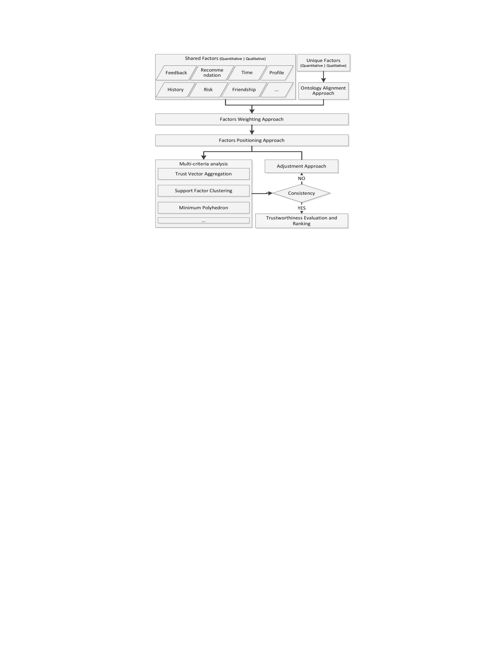
Figure 2-1 Trustworthiness measurement model (Wang and Zhengping 2014)
2.2.1 CSP evaluation and selection with fuzzy logic based trust models
Trust has become important with respect to selecting cloud services and cloud service
providers (CSPs) (Wu and Zhou 2016). However, evaluating and comparing their
trustworthiness is a challenge for cloud service customers (CSCs). Multiple approaches
have been proposed to measure trust elements and evaluate and compare cloud service
trustworthiness. A framework has been introduced that is neural network and fuzzy logic
based so that user subjective “composite criteria, feedback based learning and
inaccuracy” can be handled to evaluate trustworthiness (Wu and Zhou 2016).
Security issues impacting “data confidentiality and integrity have introduced a trust
deficit” between cloud service providers (CSPs) and cloud service users (CSUs)
(Mitchell, Rizvi and Ryoo 2015). Establishing a trust model is required to influence CSP
reputations. To establish trust, security concerns need to be evaluated. Examples of key
security issues include “lack of security standards, lack of SLAs” (Mitchell, Rizvi and
Ryoo 2015). Related to service level agreements (SLAs), generalizing SLAs can
negatively influence the “reliability of CSPs” (Mitchell, Rizvi and Ryoo 2015). To handle
22

the “subjectivity of CSUs and uncertainties associated with measuring trust,” a fuzzylogic
based trust model was proposed to evaluate CSP security according to a number of factors
(Mitchell, Rizvi and Ryoo 2015). The trust model measures both direct trust and indirect
(based on recommendations) trust. The model allows for weighting of trust evaluation
factors based on importance to the CSU. When performing the security assessment, the
following four factors are used with the fuzzy-logic model to calculate the CSP security
index: compliance, access controls, auditability, encryption. With the objective of the
security evaluation to build / restore trust between the CSP and CSU, the trust model
enables the CSU to identify the most trustworthy CSP based on their evaluation and needs
(Mitchell, Rizvi and Ryoo 2015).
A concern among cloud consumers is that critical requirements (e.g. privacy, cloud
service provider reputation) are not considered when selecting cloud services (Qu, Wang
and Orgun 2013). Cloud consumers also want to understand quality of a cloud service and
how it is evaluated (Qu, Wang and Orgun 2013). Instead, emphasis is placed on
performance analysis based on “monitoring and benchmark testing” (Qu, Wang and
Orgun 2013). In addition, benchmark testing results may not represent actual cloud
service performance based on real users. This can be due to many constraints such as
cost, simulated tasks, limited number of tests, qualitative aspects of a cloud service. A
model has been proposed for selecting cloud services based on combining feedback from
cloud users and performance testing and analysis from a trusted third party. The model
classifies and aggregates assessments (subjective and objective), then applies a fuzzy
weighting system. The model also filters unreasonable user feedback before aggregation.
The quantitative results from the model represent the cloud service quality. Figure 2-2
illustrates the cloud selection framework (Qu, Wang and Orgun 2013):
23
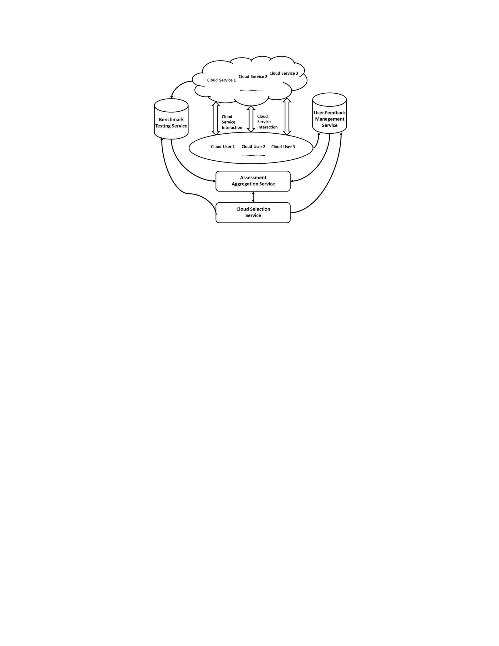
Figure 2-2 Cloud service selection framework (Qu, Wang and Orgun 2013)
Trust helps cloud service customers (CSCs) estimate a cloud service providers (CSPs)
competency to complete tasks in a cloud environment (Supriya, Sangeeta and Patra
2015). To assist CSCs when selecting a CSP, a “trust evaluation framework” is required
(Supriya, Sangeeta and Patra 2015). If the wrong CSP is selected, quality of service,
service fulfillment, security and governance of data and applications can be impacted. To
assess and rate CSPs, a “fuzzy Analytical Hierarchical Process (AHP) based hierarchical
trust model” has been proposed (Supriya, Sangeeta and Patra 2015). The approach
leverages a metric system to measure the quality of CSPs and rank the CSPs. The metrics
include accountability, agility, assurance, finance, performance, security and privacy,
usability. Fuzzy AHP supports weights assigned to the parameters and a range of values
for the hierarchical structure, resulting in improved trust estimates versus using AHP
alone. Figure 2-3 represents the relationship between parameters, attributes and trust
values. The representation helps depict the AHP evaluation as it starts from the leaf level
then continues to the next level, applying the outcome from the lower level (Supriya,
Sangeeta and Patra 2015).
24
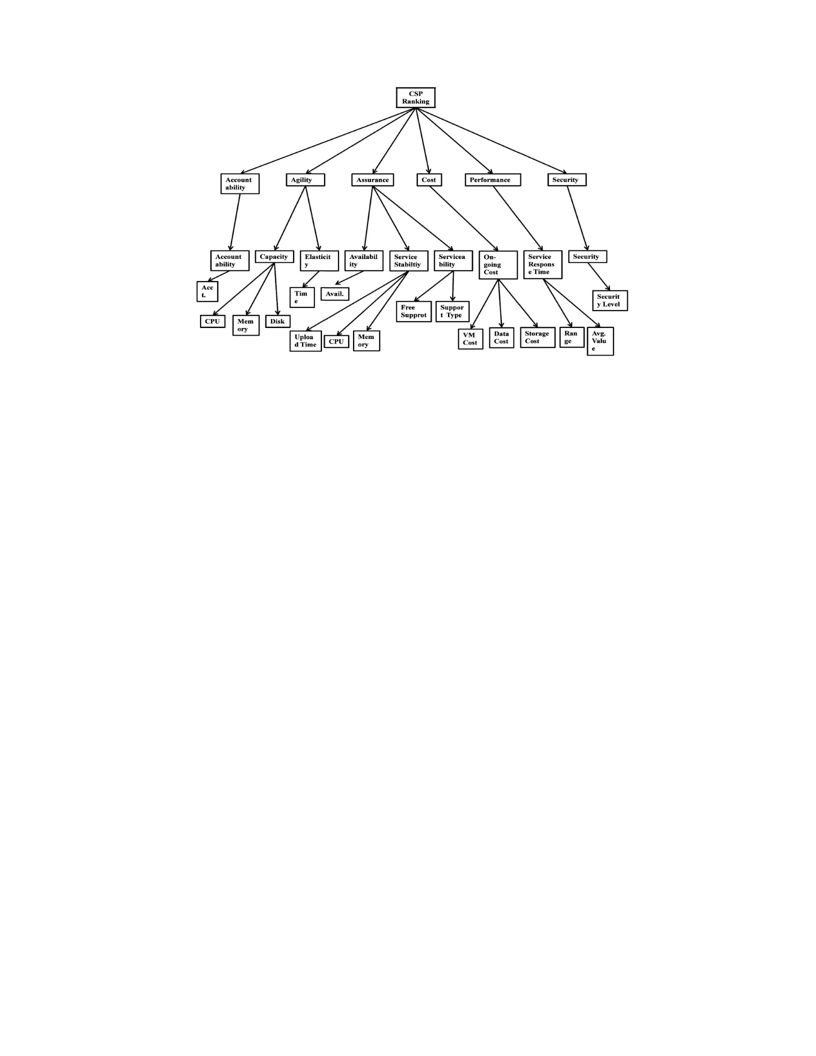
Figure 2-3 AHP Hierarchy - Relationship between parameters, attributes and trust values
(Supriya, Sangeeta and Patra 2015)
2.2.2 CSP assessment based on security capabilities
Cloud service customers (CSCs) are worried about which cloud service and cloud
service provider (CSP) they can trust (Kanpariyasoontorn and Senivongse 2017). With
the demand for cloud computing and the number of available CSPs, cloud service quality
attributes influence the CSP selection criteria. A CSP assessment method has been
proposed that focuses on cloud trustworthiness, comprising “security and dependability
attributes and six sub attributes, (i.e. confidentiality, integrity, availability, reliability,
safety, and maintainability)” (Kanpariyasoontorn and Senivongse 2017). The method is
based on the Cloud Security Alliance (CSA) Cloud Controls Matrix (CCM) with mapping
to industry standards (e.g. NIST SP 800-53 security and privacy controls, AICPA Trust
Service Principles and Criteria). The mapping serves to “classify security and
dependability characteristics of each control” (Kanpariyasoontorn and Senivongse 2017).
Leveraging the CSPs reported CSA Consensus Assessments Initiative Questionnaire
25
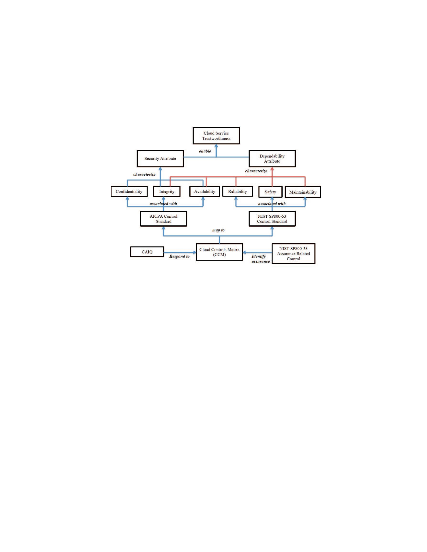
(CAIQ) and the CCM mapping, a trustworthiness score for the CSP’s cloud service is
calculated. The score can then be used when assessing and selecting
CSPs. Figure 2-4 provides an overview of the trustworthiness assessment method
(Kanpariyasoontorn and Senivongse 2017).
Figure 2-4 Cloud trustworthiness assessment method (Kanpariyasoontorn and Senivongse
2017)
While security assurance of cloud service providers (CSPs) continues to be a concern,
developments and specifications are occurring regarding security statements in service
level agreements (known as Security Level Agreements or SecLAs). CSPs are beginning
to create and store SecLAs in public repositories such as Cloud Security Alliance’s
Security, Trust & Assurance Registry (CSA STAR). To provide security assurance for a
CSP, SecSLAs need to be quantitatively reasoned. A method has been proposed to
benchmark CSP cloud SecLAs both quantitatively and qualitatively with respect to user
requirements. The methodology establishes “Quantitative Policy Trees (QPT)” which
present a data structure to represent and analyze cloud SecLAs (Luna, Langenberg and
26
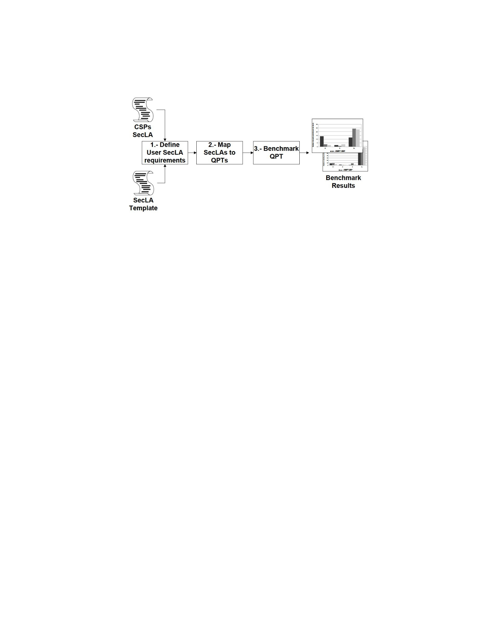
Suri 2012). The benchmark methodology is illustrated by Figure 2-5 (Luna, Langenberg
and Suri 2012):
Figure 2-5 Stages of benchmark methodology for analyzing CSP SecLA (Luna, Langenberg and
Suri 2012)
Assessing the level of security promised versus delivered by cloud service providers
(CSPs) is a challenge. While CSPs want to be trusted, customers want to evaluate and
confirm the CSP’s security assertions. With service level agreements (SLAs), we can
clarify the guarantee between a service provider and users. With the emerging industry
security level agreement (SecLA), security extensions are being introduced to cloud
SLAs along with methods to quantify CSP security assurances. These security extensions
represent a group of security declarations (i.e. service level objectives) the CSP will
provide. A framework has been proposed with a technique for performing quantitative
and qualitative analysis of CSP security level objectives. The CSP’s security capabilities
(i.e. security controls and policies) are self-assessed and published in a database managed
by the Cloud Security Alliance (CSA). The methodology leverages analytic hierarchy
process (AHP) to compare and benchmark the published CSP security capabilities against
SecLAs and then rank the CSPs. The methodology also provides customers with a means
27
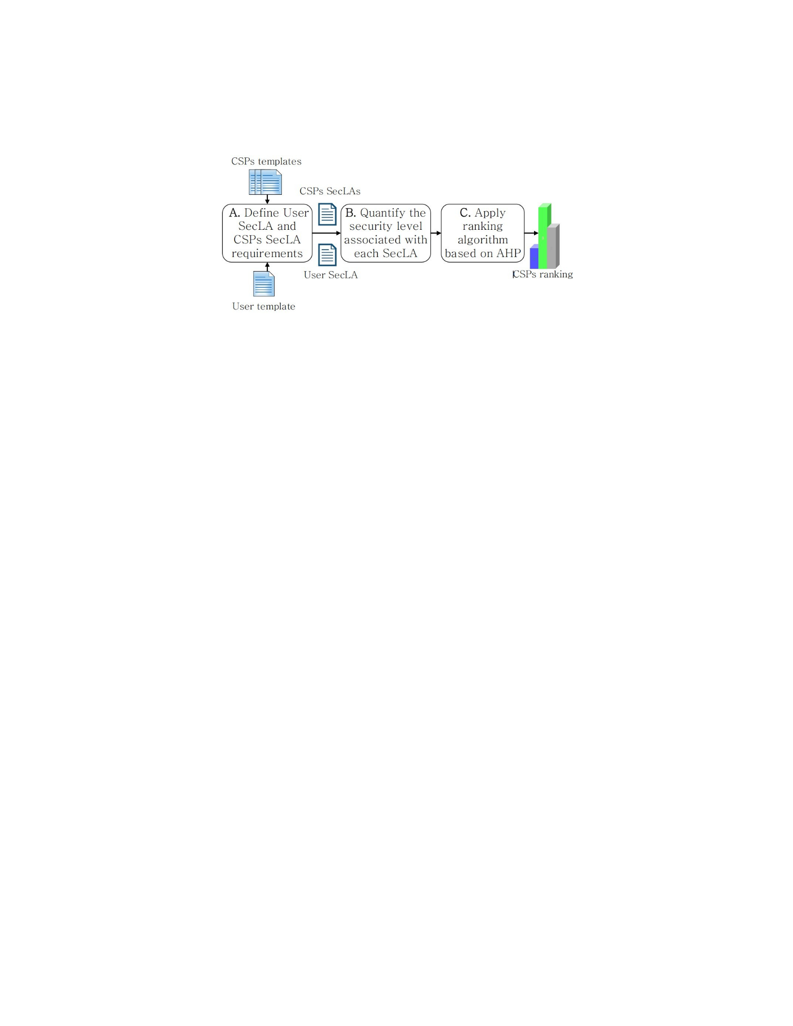
to identify their security requirements. Figure 2-6 depicts the proposed framework for
assessing and ranking CSPs (Taha et al. 2014).
Figure 2-6 Framework stages for assessing SecLA and ranking CSP (Taha et al. 2014)
Cloud service provider (CSP) trust is influenced by “security assurance and
transparency,” both of which have impacted cloud adoption (Luna et al. 2015). While
efforts in the cloud community to specify CSP security capabilities via Security Level
Agreements or secSLAs have helped, issues have impacted their adoption. Customers
want to assess and be assured that a CSP meets their security requirements. Two
techniques, Quantitative Policy Trees (QPT) and Quantitative Hierarchical Process
(QHP), have been developed for evaluating CSP secSLAs against cloud customer security
requirements. To assess the security levels, the techniques quantify and aggregate secSLA
elements. Figure 2-7 depicts the hierarchical structure of Cloud secSLAs used by the
security evaluation techniques (Luna et al. 2015).
28
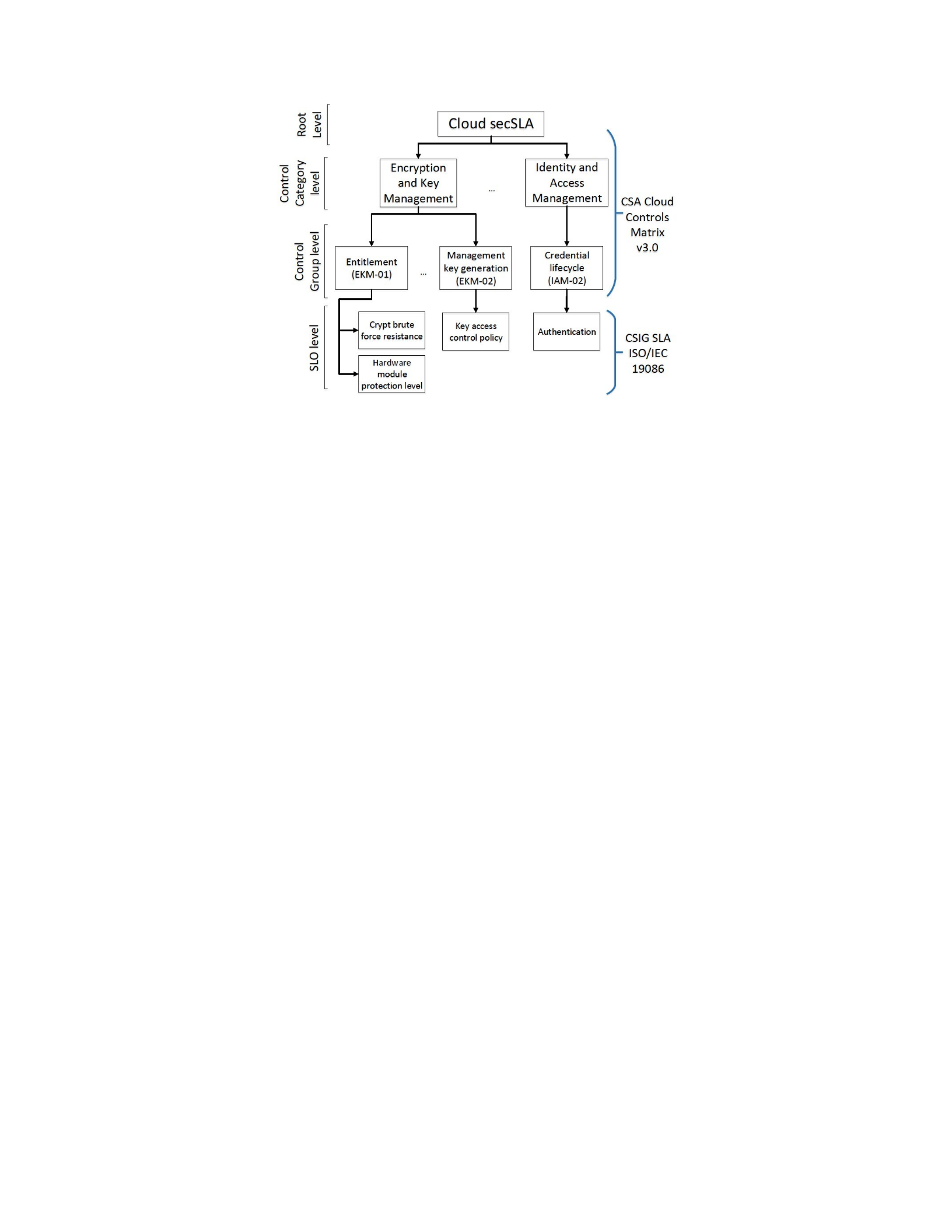
Figure 2-7 Hierarchical structure of the Cloud secSLA (Luna et al. 2015)
Selecting trustworthy cloud services from multiple cloud service providers (CSPs) is a
“challenge in the cloud computing market” (Almanea 2014). To provide the appropriate
assurance to cloud customers, CSP security compliance and historical performance must
be assessed. A trust framework called CloudAdvisor has been proposed to assure
customers by bringing transparency (i.e. disclosure) to the CSP’s claims, and enable
customers to select the CSP that fulfills their needs. The framework combines two
measurements: trustworthiness and transparency. Trustworthiness is based on CSP history
(e.g. data loss, outages, security and privacy breaches). The framework requires evidence
from CSPs (e.g. making the evidence available on a trusted third party website).
Transparency is based on the Cloud Controls Matrix (CCM) framework from the Cloud
Security Alliance (CSA) and the CSP’s compliance with CCM. CCM provides primary
security principles and documents security controls. Related to the CCM, CSA developed
the Consensus Assessments Initiatives Questionnaire (CAIQ) which can assist customers
and auditors when assessing CSPs. CloudAdvisor assesses the CSP’s transparency via a
scorecard related to the CAIQ (Almanea 2014).
29

There are many pitfalls to reliably monitoring and identifying trustworthy cloud
service providers (CSPs) based on customer requirements. Examples of concerns based
on surveys include cloud data storage locations, access to data, facility security. Service
level agreements (SLAs) are incorporating descriptions of preventative privacy and
security measures. However, SLAs alone are unclear in terms of vague clauses and
ambiguous technical specifications, and undependable by themselves for identifying
trustworthy providers. Trust and reputation systems also provide sources of information
(e.g. customer feedback, compliance with audit standards, certification) that can assist
customers when selecting trustworthy CSPs. However, all sources are not always
standard and trustworthy. Entrusted Trust Management (ETM) is an architecture that has
been introduced to reliably support customer selection of trustworthy cloud service
providers (CSPs). The architecture also provides customers with the ability to weight
sources of information that advise on CSP quality of service (QoS). ETM represents trust
as multidimensional with multiple attributes and trusted sources (e.g. Cloud Security
Alliance Consensus Assessments Initiative Questionnaire, CAIQ, that provides trust
information from CSPs). When assessing CSPs, ETM measures trust across specific
domains then overall trust based on the domains. Customer and expert ratings and
feedback are collected and the amount of conflict is measured. Trustworthiness of
information sources which provide CSP ratings based on SLAs is also measured. Figure
2-8 provides an overview of ETM (Roy, Sarker and Hashem 2015).
30
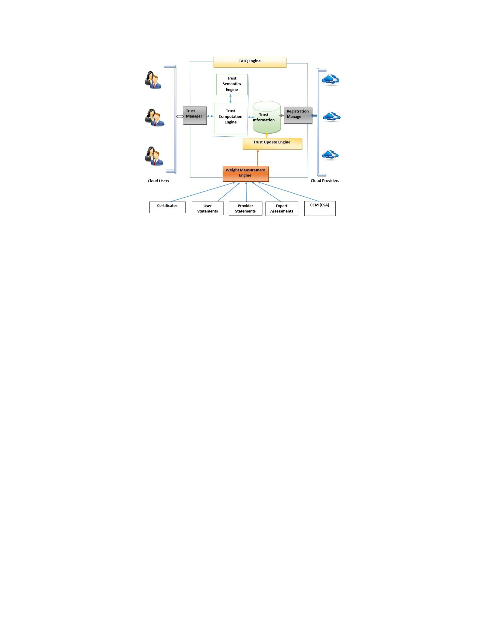
Figure 2-8 Entrusted Trust Management (ETM) architecture for supporting selection of
trustworthy CSPs (Roy, Sarker and Hashem 2015)
2.2.3 CSP selection based on QoS and SLA requirements
Based on the number of cloud service providers (CSPs) and rigid competition, CSPs
need to meet cloud service user (CSU) requirements, delivered at the CSU’s expected
level. While there are a number of criteria for selecting a trustworthy CSP, ultimately the
CSU will have their own preferences and priorities. A model has been introduced that
focuses on best fit for the CSU when assessing CSP trustworthiness and efficiency. The
model provides selection attributes and the capability for CSU weighting of the attributes.
Furthermore, the model leverages CSP provided quality of service (QoS) to enable the
CSU to evaluate the CSP based on reputation. The data for the model comes from
regulatory authorities, performance during the last year and customer feedback.
Regarding QoS, the model focuses on availability of service utilizing the following
attributes: fault tolerance, down time, up time, customer support, capability and latency
(response time). Other selection attributes introduced but not covered by the model
31

include security measures and adherence to regulatory body’s standards (Naseer, Jabbar
and Zafar 2014).
Cloud service levels and quality of service (QoS) are of chief significance to
customers (Ghosh, Ghosh and Das 2015). Service level agreements (SLAs) document the
cloud service level and QoS customer requirements and cloud service provider (CSP)
obligations. However, SLAs are not common across CSPs, making CSP selection
challenging for customers. Establishing a consistent group of parameters for cloud SLAs
is critical to lessen the perception of risk. Selecting the best CSP translates to
“trustworthy” and “competent” (Ghosh, Ghosh and Das 2015). A framework has been
proposed to assist with CSP selection by estimating risk resulting from interaction. The
estimate (i.e. quantitative assessment of risk) is based on combining CSP trustworthiness
and competence. Trustworthiness calculations utilize customer feedback and personal
experiences related to the CSP. Capability and competency is measured based on
transparency to CSP SLAs and performance. Related to the framework and estimating
competence, a group of SLA parameters was proposed (security, compliance, data
governance, resiliency, operations management). Figure 2-9 depicts the modules of the
framework and their functional relationships (Ghosh, Ghosh and Das 2015).
32
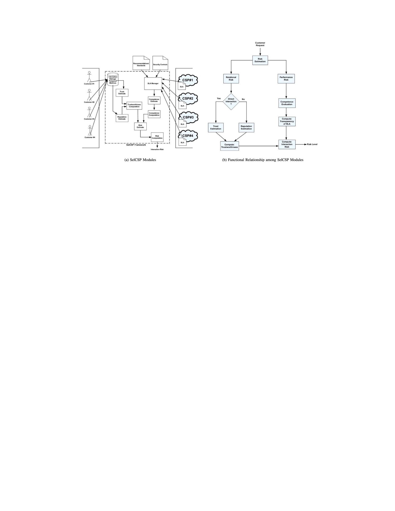
Figure 2-9 CSP selection framework module interactions (Ghosh, Ghosh and Das 2015)
High availability is a competitive guarantee between cloud service providers (CSPs).
While CSPs strive to meet that guarantee, reports assert that downtime is significantly
higher and the guarantee doesn’t always equate to service level agreement (SLA)
compliance. Deciding which CSP to select is further complicated by other challenges
(e.g. performance, security, data privacy, legal compliance, cost). To evaluate CSPs and
cloud service customer (CSC) needs, a methodology has been defined. The methodology
utilizes trustworthiness as a factor and a method for quantifying trustworthiness along
with security. To quantify CSP trustworthiness, the methodology uses availability based
on SLA guarantees and reliability (i.e. historical actual cloud availability). Other
observations related to the methodology and research noted that not all CSPs define
downtime equally (e.g. inclusion of maintenance) and that CSP trustworthiness can be
influenced by CSP security certifications (Ristov and Gusey 2015).
With service level agreements (SLAs) serving to provide levels of assurance that a
cloud service consumer’s (CSC’s) requirements are being met by a cloud service provider
(CSP), there is no single method for defining CSC service level expectations. With SLA
variations among CSPs (e.g. “description, length, and types of information released”) and
33
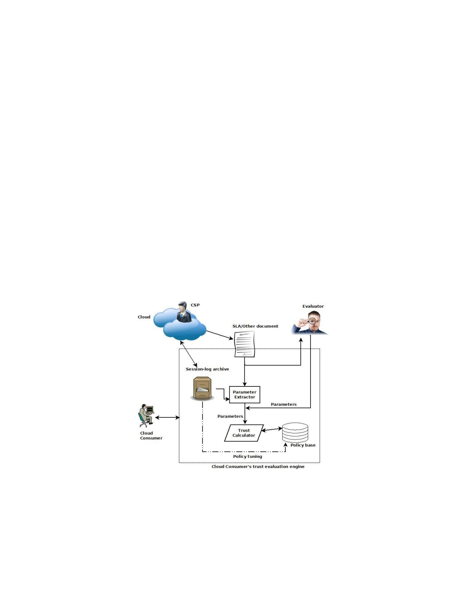
lack of a standard cloud SLA, challenges exist when estimating CSP trustworthiness
(Chakraborty, Sudip and Roy 2012). To address the challenges, a framework has been
proposed to estimate trustworthiness based on a quantitative model of trust and
formalized SLA parameters. The framework allows for weighting the parameters based
on importance levels to the CSC. Some of the parameters used to estimate trust relate to
different properties of the cloud service and can be assessed before an SLA is signed (e.g.
backup frequency, CPU capacity, mean-time-to-recovery, memory size, number of
parallel sessions, storage capacity). Other parameters relate to CSP performance and the
SLA between the CSP and CSC. These parameters can be collected and evaluated from
session histories or logs after the SLA has been signed (e.g. total time to complete a job,
average throughput related to data exchanged). Figure 2-10 depicts the proposed trust
estimation framework (Chakraborty, Sudip and Roy 2012).
Figure 2-10 Architecture of the CSP trust estimation framework (Chakraborty, Sudip and
34

Roy 2012)
Cloud service customers (CSCs) lack capabilities to verify the behavior of the CSP
(Ruan et al. 2016). They are left with indiscriminately believing the CSP won’t modify
their data and that levels of assurance are enforced. As a result, CSP’s governance and
lack of transparency within the cloud impacts CSP trust levels. Even various cloud
auditing schemes enforced by recognized and trusted authorities (e.g. government
agencies) may not reflect the most current status of a cloud infrastructure nor the most
complete information to prove the existence of trust. This makes it difficult for CSCs to
confirm whether their service level agreements (SLAs) have been satisfied and their
requirements have been met. The assertion is that the trust issues are caused by a CSPs’
excess authority. A Separation-of-Powers (SoP) model has been proposed to separate a
CSP’s authorities thereby increasing the trustworthiness of the cloud service provider
(CSP). The model introduces three roles to separate powers and achieve “balance-
ofpowers” from the CSP: definition, enforcement, and inspections (Ruan et al. 2016).
The roles can then be provided by multiple, competing third parties with enforcement of
collaboration and restriction dynamics among the roles. The outcome of the model is a
cloud ecosystem that is trustworthy and open (Ruan et al. 2016).
2.3 Cloud monitoring and trust levels based on QoS and SLAs
With the growth of cloud computing, service level agreements (SLAs) and standard
security requirements are “one of the most important issues influencing further adoption”
(Hogben and Dekker 2012). It’s important to not only identify the requirements
immediately, but also track and validate they are being met. A framework has been
provided related to purchasing and managing cloud services and monitoring of security
requirements (including availability and service continuity). The goal is to establish
35

awareness and increased comprehension of cloud services, security and assessments. To
ensure proper controls and procedures are in place, assessments of cloud service
providers (CSPs) are critical. However, since assessments don’t provide live information
nor alerts based on thresholds, they are inadequate. The framework describes the
parameters that should be monitored, how to collect the data and measure the parameters,
when to set alert thresholds and reporting, and customer duties. The parameters cover the
following: service availability, incident response, service elasticity and load tolerance,
data life-cycle management, technical compliance and vulnerability management, change
management, data isolation, log management and forensics. When selecting parameters
and which ones SLA monitoring will focus on, organizations should analyze risk and
impact related to their mission, use-cases, and characteristics of the cloud services
(Hogben and Dekker 2012).
Provisioning cloud services is based on service level agreements (SLAs). For
example, SLAs confirm terms, obligations and quality of service (QoS) requirements
between the customer and cloud service provider (CSP). Managing and enforcing SLAs
require a framework for monitoring low-level objects and correlating with application
specific SLA attributes (e.g. application availability). A framework (LoM2HiS) has been
proposed for managing Low-level resource metrics mapped to High-level SLAs. The
framework is the autonomic part of a broader framework (FoSII from Vienna University
of Technology) that provides a model for SLA management and enforcement. The
LoM2HiS framework detects SLA violations and provides the appropriate notification.
To detect future SLA violations, the LoM2HiS proposes threat levels that are with more
restrictions than normal SLA violation levels. Figure 2-11 represents the framework
(Emeakaroha et al. 2010).
36
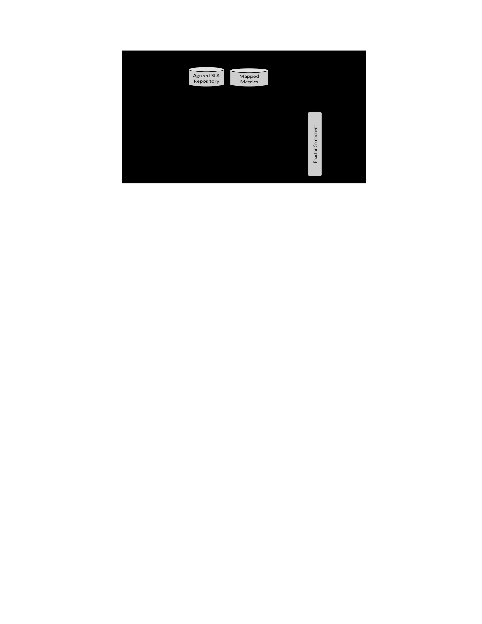
Figure 2-11 Framework architecture for managing low-level resource metrics to high-level
SLAs (Emeakaroha et al. 2010)
Concerns related to privacy, security and trust influence the adoption of cloud
computing (Muchahari and Sinha 2012). Furthermore, self-proclaimed levels of
trustworthiness by cloud service providers (CSPs) have not improved cloud service
consumer’s (CSC’s) trust of CSPs. Some of the parameters that influence and establish
CSC trust of the CSP include “quality of service (QoS), service level agreement (SLA),
performance test, user recommendation, feedback and publicly available reviews,
compliance, … security measures” (Muchahari and Sinha 2012). A trust management
architecture has been proposed that calculates CSP trust values based on feedback related
to CSP SLAs and QoS. The architecture includes “Cloud Service Registry and
Discovery” where the CSP trust values are registered and listed (Muchahari and Sinha
2012). The architecture also monitors trust value dynamics as influenced by time and
transactions since QoS and SLA requirements change due to changing dynamics of cloud
business operations and operating environments. Figure 2-12 represents the proposed
model for registering and monitoring CSP trust values (Muchahari and Sinha 2012).
37
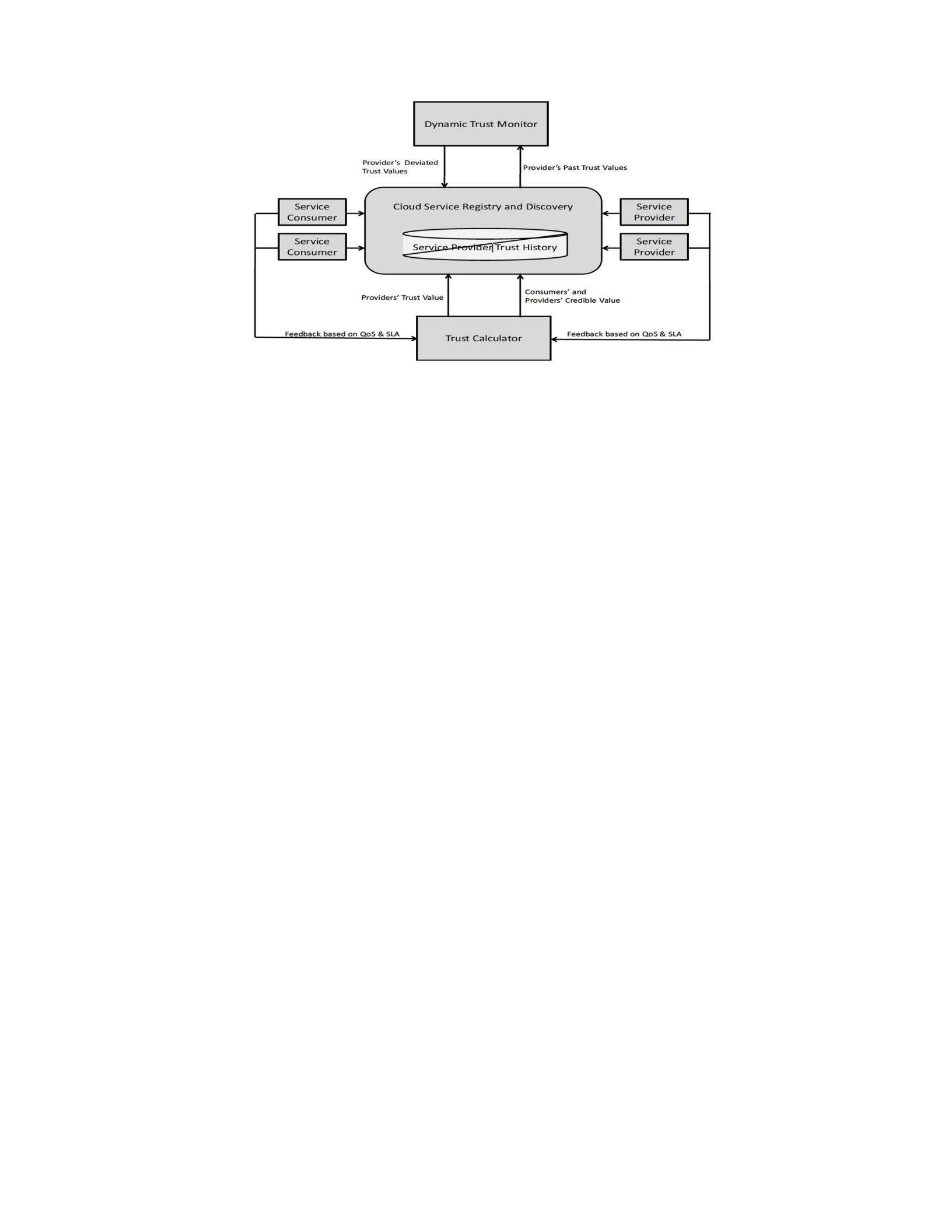
Figure 2-12 “Cloud Service Registry and Discovery with Trust Calculator and Dynamic
Trust Monitor” (Muchahari and Sinha 2012)
Cloud service provider (CSP) trust has been identified as a grave issue with respect to
cloud computing (Manzoor, Taha and Suri 2016). In terms of customer requirements, trust
is defined as the extent of dependability on CSP services. To address the trust concern,
CSPs have established service level agreements (SLAs) that confirm their obligations
with respect to customer requirements. However, limitations related to validating SLA
compliance impact the ability to evaluate CSP trust. A methodology has been proposed to
validate SLAs and confirm any violations. The validation considers SLA attributes (i.e.
measurable characteristics) that are essential to the customer and committed by the CSP.
The assessed attributes can be both qualitative and quantitative. Based on the severity
level of the violation (i.e. impact based on extent of violation) and customer
requirements, the CSP is placed into a “trust state,” which represents the extent of SLA
violation (Manzoor, Taha and Suri 2016). Figure 2-13 depicts the stages of the
methodology for identifying the “trust state” (Manzoor, Taha and Suri 2016).
38
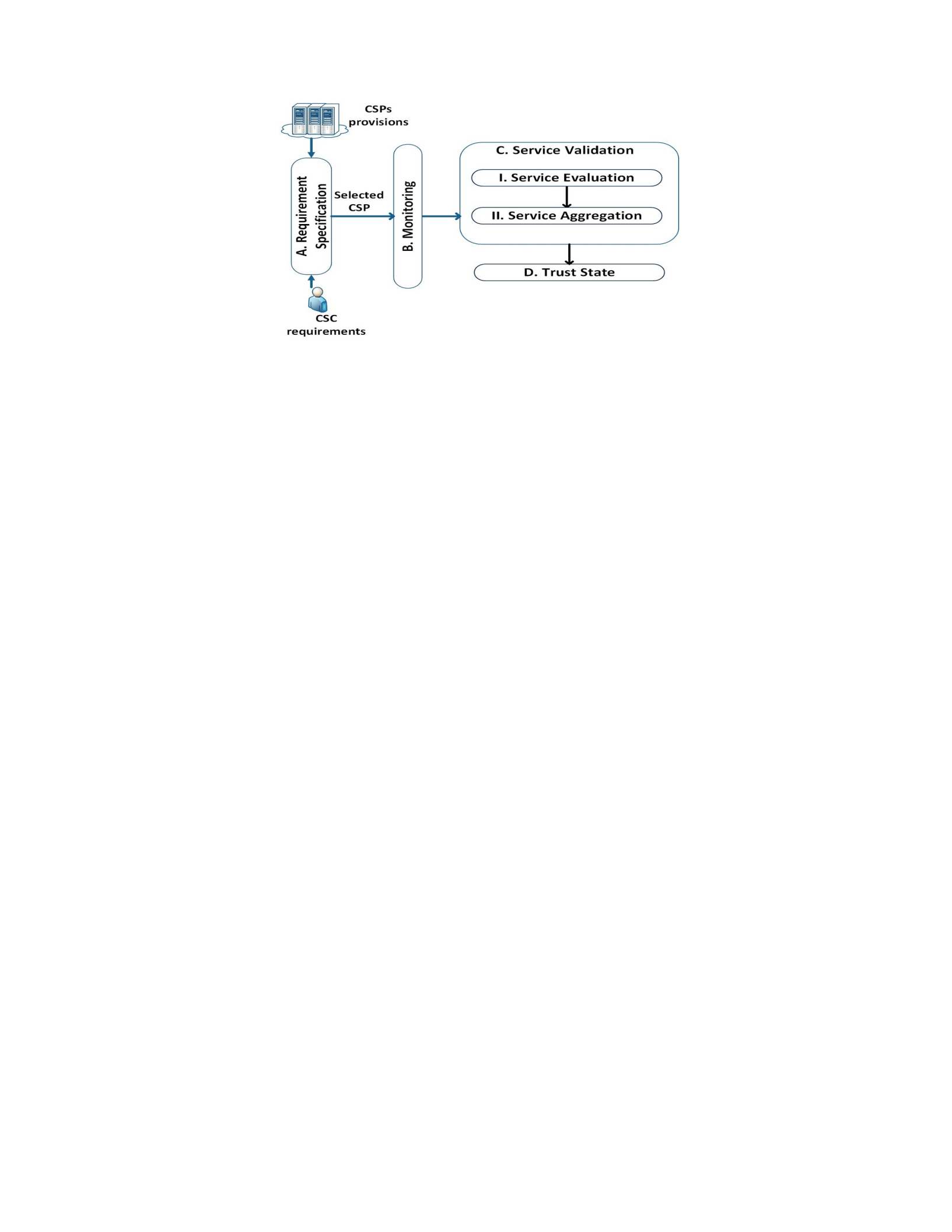
Figure 2-13 Stages of the methodology for identifying the CSP “trust state” (Manzoor, Taha and
Suri 2016)
An outstanding key cloud computing issue that needs to be addressed is service level
management (Hammadi and Hussain 2012). Service level management ensures that cloud
services meet service level agreement (SLA) specifications and criteria of the cloud
service customer (CSC). Failing to manage and assure quality of service (QoS) at the
agreed service levels results in reduction in quality of cloud services. QoS represents a
quality metric related to benchmarking a cloud service. To assess real-time QoS and the
assurance of meeting CSC SLA specifications, a SLA monitoring framework is proposed.
The proposed framework (which needs to “take into account the self-service and
ondemand nature of the cloud”) is a third-party SLA monitor that consists of two
assessment modules: reputation assessment and transactional risk assessment (Hammadi
and Hussain 2012). Reputation, interrelated and complimented with trust, are QoS
parameters that measure confidence level and expected financial impact associated with
the cloud service provider. The benefit of the SLA monitoring framework combines
realtime QoS assessment along with user feedback regarding quality of service delivered
by the cloud service provider (Hammadi and Hussain 2012).
39

Ensuring solid operations for cloud computing data centers and infrastructure requires
continuous monitoring. Unfortunately, monitoring approaches can be ad hoc, producing
inconsistent quality. Monitoring alerts tend to be “reactive in nature,” resulting in limited
time for only “quick work-arounds and fixes” (Natu et al. 2016). Ideally the “ability to
predict and generate preventative alerts” is what’s required to “avoid the problem in the
first place” (Natu et al. 2016). One approach identifies dependencies, correlation and
regression models. Simulation can then be used to predict system variables and anticipate
their effect on the system (Natu et al. 2016).
2.4 Cloud SLA enforcement through proactive QoS and autonomic computing
While phase 4 of the Cloud SLA Lifecycle is not in within the scope of the proposed
solution, it is indirectly related to phases 1 through 3. To provide a complete view of the
cloud SLA lifecycle, phase 4 is being introduced in this Praxis. Refer to Appendix L for
details.
Chapter 3. Methodology
3.1 Research Goals
The overall goal of the research was to utilize multiple methodologies to analyze,
model and predict cloud industry service level agreement performance based on a number
of factors. Examples of the factors include service level agreement (SLA) standards,
cloud service provider (CSP) trustworthiness, and historical CSP cloud service
performance and cloud service characteristics. As previously noted, the following
objectives were established to drive the research methodology.
•To assess industry related cloud SLA standards and structures.
40

•To define a CSP trustworthiness framework based on analysis of CSP compliance
with the cloud SLA standards and security frameworks and establish CSP trust
levels.
•To develop a model for predicting cloud SLA performance (i.e. cloud service
Availability) based on a standard cloud SLA structure, CSP trustworthiness, and
historical CSP cloud service performance and characteristics.
•To evaluate and validate the predictive model, and assess the observations and
predictions related to predicting cloud SLA performance (i.e. cloud service
Availability).
The multiple methodologies utilized by the research included Graph Theory, Analytic
Hierarchy Process (AHP) and Linear Regression Analysis. The expected composite
outcomes from the methodologies served to support the hypothesis testing and results.
Each of the following summaries highlight data flow dependencies between the
methodologies. A methodology map (Figure 3-1) has been provided in the next section of
this chapter to model these dependencies.
•Graph Theory was used to model, analyze and compare cloud SLA structures and
cloud security controls based on industry standards and guidelines, and CSP SLA
structures (Roberts 1978). The cloud industry SLA standards and guidelines
originated from the International Organization for Standardization / International
Electrotechnical Commission (ISO/IEC) (ISO/IEC 2016), European Commission
(EC) (EC 2014), and European Union Agency for Network and Information
Security (ENISA) (Hogben, Giles and Dekker 2012). The CSP SLAs were taken
from the top three market leaders: Amazon, Google, Microsoft. Modeled cloud
security specific controls originated from the Cloud Security Alliance (CSA)
41

Cloud Controls Matrix (CCM) (CSA CCM 2017) and CSP assessments from the
CSA Security, Trust and Assurance Registry (STAR) and Consensus Assessments
Initiative Questionnaire (CAIQ) (CSA STAR 2017). With the graphical model and
analysis, areas of focus, differences and overlaps were identified and illustrated.
The result of the analysis served as input to the Analytic Hierarchy Process for
calculating CSP trustworthiness.
•Analytic Hierarchy Process was used to model and assess CSP trustworthiness
based on CSP SLA and security related capabilities. CSP historical SLA and cloud
service resource performance was factored into the trustworthiness. AHP analysis
leveraged existing published research (Supriya, Sangeeta and Patra 2015, Taha et
al. 2014, Luna, Langenberg and Suri 2012, Luna et al. 2015) that previously
focused on security controls. The existing research was extended to include AHP
analysis of security controls in addition to all SLA capabilities plus historical SLA
performance. The CSP SLA historical performance was provided by industry
analyst Gartner’s Technology Planner Cloud Module, renamed Cloud Decisions
(Gartner 2017). The Gartner Technology Planner Cloud Module provided
historical CSP cloud service performance data for SLA and cloud service
resources (e.g. cloud service availability; networking latency and throughput;
utilization for CPU, storage, memory and network; provisioning). With AHP,
industry cloud SLA standards, historical SLA performance and CSA security
capabilities were quantified, weighted and assessed for each CSP. The results of
the comparisons were aggregated and CSPs were ranked. CSP trustworthiness
was calculated based on the ranking.
42

•Linear Regression Analysis was used to model and predict SLA performance (i.e.
Availability) and to test the hypothesis. The predictive modeling utilized CSP
trustworthiness levels in addition to historical CSP cloud service performance data
from Gartner’s Technology Planner Cloud Module (Cloud Decisions) (e.g. cloud
service downtime; networking latency and throughput; utilization for CPU,
storage, memory and network; provisioning turnaround).
To validate the models, Goodness of Fit was evaluated in addition to assessing the
value of the models at addressing the hypothesis. The SLA performance calculations and
predictions produced by the models as a result of the linear regression analysis were
validated to determine if they accurately reflected the true outcome experience in the
data, and if they enabled accurate testing of the hypothesis. ANOVA F-test was performed
to compare the simple and multiple linear regression models and confirm whether the
additional regression coefficients from the multiple linear regression model provided
explanatory and/or predictive power to the model.
To influence the accuracy and reliability of the model, data set, and hypothesis testing,
the performance data input into the model is based on actual historical SLA and cloud
service performance from the CSPs Amazon, Google and Microsoft. The CSP
trustworthiness levels being used by the model were calculated based on real CSP
historical SLA performance in addition to real CSP SLA definitions and self-assessments
concerning their security capabilities from the CSA Security, Trust and Assurance
Registry (STAR) and Consensus Assessments Initiative Questionnaire (CAIQ) (CSA
STAR 2017).
43

3.2 Research Methods
The research method involved three key methodology phases as depicted by the
methodology map diagram in Figure 3-1. The methodology map serves to identify the
data sources, methodologies, their relationships and how they support hypothesis testing.
The methodology phases included: Graph Theory, Analytic Hierarchy Process (AHP) and
Linear Regression Analysis.
Starting at the top of Figure 3-1 Methodology Map, the first phase of the research
begins with multiple cloud related organizations (e.g. ISO/IEC, EC, ENISA, CSA,
Amazon, Google, Microsoft) providing data for Graph Theory analysis (red box). Graph
Theory was leveraged to model, analyze and compare the cloud organizations, cloud
SLAs and cloud security controls. The cloud SLAs were developed by industry standards
organizations EC, ENISA and IEC/ISO (EC 2014, Hogben, Giles and Dekker 2012,
ISO/IEC 2016), and CSPs Amazon, Google and Microsoft (SLA AWS 2017, SLA Google
2017, SLA Microsoft 2017). The cloud security controls or CCM (CSA CCM 2017), were
identified by CSA, with CAIQ (CSA CAIQ 2017) compliance results completed for CSPs
Amazon, Google and Microsoft (STAR AWS 2017, STAR Google 2017, STAR Microsoft
2017). The CAIQ results for all CSPs are stored in the CSA’s STAR (CSA STAR 2017).
Output from the Graph Theory phase models requirements and controls related to
industry cloud SLAs and cloud security controls, and serves as input to the AHP phase
noted on Figure 3-1.
The second phase as depicted on Figure 3-1 Methodology Map, utilized AHP (blue
box) to further analyze and then rank each CSP in terms of trustworthiness. The analysis
and ranking was based on the CSP’s SLA and security capabilities contrasted against
industry standard cloud SLAs and security controls modeled by phase one Graph Theory.
44

CSP historical data from Gartner (Gartner 2017) regarding SLA performance was also fed
into the AHP analysis and calculations (see Figure 3-1 Gartner data source input to AHP
of CSP SLA performance and CSP number of service regions). The AHP analysis and
ranking was ultimately utilized to calculate CSP trustworthiness as input to the third
phase on Figure 3-1, Linear Regression.
The third phase depicted on the bottom left of Figure 3-1 Methodology Map utilized
Linear Regression Analysis (green box) to examine the relationships between multiple
CSP cloud service variables, their related observations and CSP trustworthiness. The
result of the analysis of the relationships produced linear regression models (i.e. Simple
and Multiple) to predict SLA performance for cloud compute services and test the
Hypothesis. The cloud service and CSP variable and observation data was based on actual
cloud service configurations and performance from real CSPs (i.e. Amazon, Google,
Microsoft). As depicted on Figure 3-1, Gartner’s Technology Planner Cloud Module
provided Linear Regression with CSP cloud service SLA and network performance data,
in addition to CSP data center and service region data (Gartner 2017). The CSP cloud
service variables were related to SLA availability and cloud service downtime
performance, network performance (i.e. latency and throughout), characteristics regarding
global cloud service hosting centers. CSP trustworthiness levels for Amazon, Google and
Microsoft from phase two (AHP box on Figure 3-1) were also input into the linear
regression analysis and related to the SLA performance calculations and predictions.
45
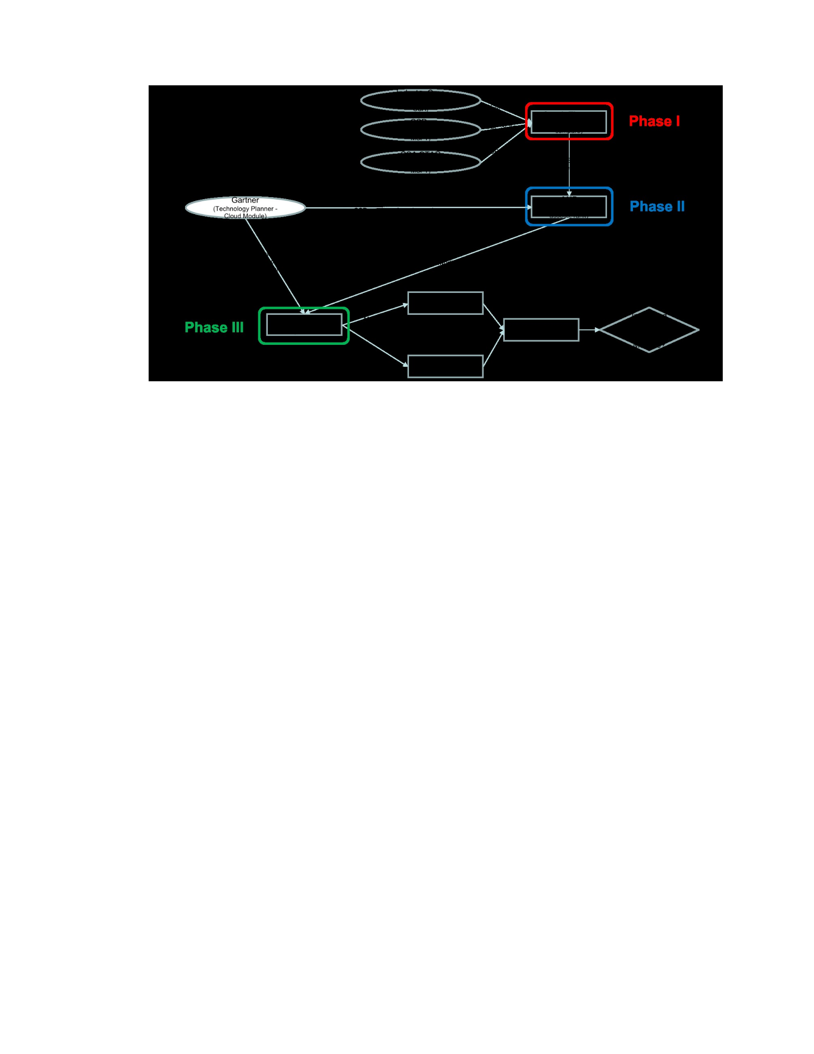
Figure 3-1 Methodology Map
3.3 Research Plan
3.3.1 Graph Theory to Model Cloud SLAs and Security Controls
A graph is an efficient way to describe a network structure and represent information
about relationships between nodes (e.g. organizations). With a graph, key features can be
identified such as whether all the nodes are connected. Are there subgroups or clusters of
nodes that are tied together but not to other subgroups? Which nodes have more
relationships (ties) than others? The graph can help us understand the nodes, their
connections to one others, and the role the node plays in the overall structure.
Graph Theory was used for this research to model cloud SLA work driven by industry
standards organizations (EC, ENISA, ISO/IEC) (EC 2014, Hogben, Giles and Dekker
2012, ISO/IEC 2016) and how it related to the cloud SLAs provided by the top three
CSPs (Amazon, Google, Microsoft) (SLA AWS 2017, SLA Google 2017, SLA Microsoft
2017), along with cloud security controls from CSA (CSA CCM 2017). With the modeled
graphs, gaps, overlaps and relationships between the organizations were illustrated.
46

Supporting details related to the SLA and security capabilities was provided in
Appendices B, C, E. The primary goal was to analyze and confirm the SLA and security
structure that would be input to the Analytic Hierarchy Process and be used for
calculating CSP trustworthiness, which ultimately was input to the Linear Regression
based predictive model.
NetDraw (Borgatti 2002), a network analysis software package, was used for
visualizing the industry and CSP cloud SLA and security capabilities. The network graphs
produced by NetDraw enabled a graphical depiction of the data (nodes) and strength of
the data relationships (ties…lines). Each of the graphs were directed (i.e. the ties have
direction with arrows on the lines between the nodes). Both the nodes and ties can have
different sizes depending on the type of actor for the node, strength of the relationship for
the ties, and specific criteria to each. The larger the node and thicker the line, the stronger
the representation of the criteria.
The nodes on the graphs represent multiple actors which include organizations and
data structures related to SLAs and security capabilities. The organizations were
comprised of CSPs (Amazon Google, Microsoft) and industry standards bodies (CSA,
EC, ENISA, ISO/IEC). The SLA related actors represent CSP SLAs for Amazon, Google
and Microsoft (SLA AWS 2017, SLA Google 2017, SLA Microsoft 2017), and industry
cloud SLA standards for EC, ENISA and ISO/IEC (EC 2014, Hogben, Giles and Dekker
2012, ISO/IEC 2016). The security related actors represent security control domains for
CSA CCM (CSA CCM 2017). Various colors and shapes were used for different types of
nodes to help convey information about what type of actor each node is. Delineating the
different actors helped focus on the relationships between the CSPs and standards bodies,
47

as well as CSPs with SLAs and security controls. Ultimately, these relationships with
CSPs influence the CSP’s trustworthiness level.
The CSA CCM (CSA CCM 2017) represents 16 governing and operating domains
separated into control domains and across the domains, 133 controls and 296 control
related questions. The CAIQ (CSA CAIQ 2017) provides a survey for CSPs to assess and
communicate their capabilities across all domains. The CSP CAIQ survey results are
maintained in the CSA STAR (CSA STAR 2017). Standards bodies such as EC, ENISA
and ISO/IEC are working on SLA standards (EC 2014, Hogben, Giles and Dekker 2012,
ISO/IEC 2016) for the cloud industry. The SLA standards for EC, ENISA and ISO/IEC
represent a combined set of 12 content areas and 82 components (refer to Appendix B).
When collecting the data and assessing which graphs to build, the following questions
were considered.
•What relationships exist between the CSA CCM (CSA CCM 2017) and each of
the three CSP’s CAIQ (Amazon, Google, Microsoft) (STAR AWS 2017, STAR
Google 2017, STAR Microsoft 2017)?
•How strong are the CSP (Amazon, Google, Microsoft) CCM capabilities (STAR
AWS 2017, STAR Google 2017, STAR Microsoft 2017) across each control
domain?
•Knowing the CCM control domains have some overlap with the SLA standards,
what is the relationship between CSA CCM and cloud SLA standards … where
are the gaps and how strong are the overlaps?
•What SLAs exist for each CSP (Amazon, Google, Microsoft) (SLA AWS 2017,
SLA Google 2017, SLA Microsoft 2017)?
48

•What SLAs have interrelationships across CSPs and what are the SLA gaps and
overlaps between the CSPs?
•What are the relationships between the CSP SLAs (SLA AWS 2017, SLA Google
2017, SLA Microsoft 2017), industry standards organizations and industry cloud
SLA standards (i.e. content areas) (EC 2014, Hogben, Giles and Dekker 2012,
ISO/IEC 2016)?
•What cloud SLA standards are related to what industry standards organizations
and CSPs?
The Appendices B, C, E describe the data collected and analyzed for modeling the
graphs and addressing the questions.
3.3.1.1 Industry Cloud SLA Standards
Standards bodies ISO/IEC, ENISA and EC have contributed the work outlined in
Appendix B towards standardized cloud SLAs (ISO/IEC 2016, Hogben, Giles and
Dekker 2012, EC 2014). The standardized cloud SLA content has been organized into 12
Content Areas per the SLA framework developed by ISO/IEC (ISO/IEC 19086-1 2016,
ISO/IEC 19086-2 2017, ISO/IEC 19086-3 2017). Additional cloud SLA details developed
by each standards body have been recorded in the table associated with each Content
Area: Components from ISO/IEC (ISO/IEC 19086-1), Requirements from EC (EC 2014)
and Parameter Groups (Hogben, Giles and Dekker 2012). The cloud SLA details from
each standards organization describe the content areas along with addressing cloud
services, definitions, service monitoring, and roles and responsibilities. Each Content
Area and corresponding cloud SLA details also include cloud service level objectives
(SLOs) and cloud service qualitative objectives (SQOs). The SLOs and SQOs represent
the metrics and targets CSPs can leverage when offering cloud SLAs. For each Content
49

Area, the number of cloud SLA details (i.e. Components, Requirements, Parameter
Groups) provided by each standards organization (i.e. EC, ENISA, ISO/IEC) are totaled.
These total counts are leveraged when modeling the industry cloud SLA standards graph
along with calculating the node and relationship (ties) strength.
3.3.1.2 CSP Service Level Agreements
Cloud SLAs assist CSPs in governing relationships with cloud service customers
(CSCs), documenting CSC requirement and expectations related to quality of service
(QoS), and confirming CSP obligations. The CSPs use cloud SLAs for “measuring,
monitoring and reporting the performance of the cloud” based on the CSCs consumption
of cloud resources (Mirobi and Arockiam 2015). Each CSP provides measurable details
(e.g. data rates, mean time to repair, throughput) in their SLAs that provide competitive
differentiators. The CSP SLAs are reviewed regularly with CSCs to enforce rewards and
penalties of the contract (Mirobi and Arockiam 2015).
Appendix E reviews the cloud SLAs offered by CSPs Amazon, Google and
Microsoft. The cloud SLAs offered by each CSP only focus on the standardized cloud
SLA Availability Content Area reviewed in the last section. As noted in the table along
with the total, each CSP offers multiple types of Availability SLAs. For example, all three
CSPs offer a Compute SLA where monthly uptime is defined as cloud SLA Component
detail. The detail includes the Service Level Objective (SLO) for measuring the cloud
service (e.g. CSP Availability service level commitments: Amazon >= 99.99%,
Google and Microsoft >= 99.95%) (SLA AWS 2017, SLA Google 2017, SLA Microsoft
2017).
The different types of Availability SLAs in Appendix E, both unique to the CSP
and common among multiple CSPs (e.g. Compute SLA), along with the total count of
50

SLAs are both leveraged when modeling the CSP cloud SLA graph. The total counts are
also used to calculate the node and relationship (ties) strengths between the CSPs,
different types of Availability SLAs, and industry standards organizations.
3.3.1.3 CSA CCM and CSP Compliance
The Cloud Security Alliance (CSA) is an organization established in 2008 focused on
promoting best practices for cloud computing security (CSA 2017). CSA has a number of
active work groups with research that has produced the following to assist CSCs when
assessing CSP security capabilities: Cloud Controls Matrix (CCM) (CSA CCM 2017),
Consensus Assessments Initiative Questionnaire (CAIQ) (CSA CAIQ 2017) and
Security, Trust and Assurance Registry (STAR) (CSA STAR 2017).
CCM is “designed to provide fundamental security principles to guide cloud vendors
and to assist prospective cloud customers in assessing the overall security risk of a cloud
provider” (CSA CCM 2017). CCM offers a security framework of 133 controls spread
across 16 domains. The framework endeavors to “normalize security expectations, cloud
taxonomy and terminology, and secures measures implemented in the cloud.” (CSA CCM
2017).
Consensus Assessment Initiatives Questionnaire (CAIQ) provides CSCs and cloud
auditors a set of 296 questions they can leverage to assess a CSP. The questions are
structured to represent CSC requirements and align with the CCM control domains (i.e.
16 governing and operating domains). For each control domain, the questions are
organized based on the controls within the domain. The result of the CSPs answers to the
questions (i.e. yes or no) helps ascertain the CSPs level of compliance to CCM and CSA’s
best security practices.
51

STAR is a publicly available registry provided by CSA based on CCM and CAIQ.
STAR documents security controls for various CSPs and serves to help CSCs assess the
CSP. CSPs provide completed CAIQs or reports that document CCM compliance. The
CSP submissions are freely available with the intent of promoting transparency and
visibility into CSP security practices. (CSA STAR 2017).
The CCM control domains, controls for each domain, and number of CAIQ
questions related to each control (refer to the CSA column) are represented by Appendix
C (CSA CCM 2017, CSA CAIQ 2017). Appendix C also provides a total count for each
CSP (Amazon, Google, Microsoft) of the number of questions within a control domain
and within a control the CSP answered yes (i.e. the CSP satisfies the CAIQ control
question for the CCM control domain). The control domains, controls and question
counts (CSA total and total for each CSP) are leveraged when modeling the CSA CCM
and CSP compliance graph. The total counts are also used to calculate the node and
relationship (ties) strengths between the CCM control domains and CSPs.
3.3.2 Analytic Hierarchy Process to Model CSP Trustworthiness
Cloud service customers (CSCs) want to confirm claims from cloud service providers
(CSPs) regarding the quality and security of their cloud services. Calculating and ranking
the trustworthiness of CSPs provides a means for CSCs to rank CSPs and validate their
ability to meet service level expectations (EC 2014, Hogben, Giles and Dekker 2012,
ISO/IEC 2016). To enable the assessment of CSPs, industry organizations (e.g. EC,
ENISA, ISO/IET, CSA) have introduced and are evolving standards and specifications for
capturing CSC requirements (e.g. SLAs) and measuring against CSP performance (SLA
AWS 2017, SLA Google 2017, SLA Microsoft 2017). CSA has introduced a framework
and questionnaire (CSA CCM 2017, CSA CAIQ 2017) for CSPs and CSCs to assess CSP
52

capabilities and controls related to delivering quality and secure cloud services. CSA has
established an online repository (CSA STAR 2017) where CSP CAIQ assessments are
published. While published assessments provide CSCs with transparent awareness for
individual CSP capabilities and controls, a technique is required for assessing, comparing
and ranking CSPs and ultimately calculating CSP trustworthiness (Wu and Zhou 2016,
Mitchell, Rizvi and Ryoo 2015, Qu, Wang and Orgun 2013,
Supriya, Sangeeta and Patra 2015, Kanpariyasoontorn and Senivongse 2017, Luna,
Langenberg and Suri 2012, Taha et al. 2014, Luna et al. 2015, Almanea 2014, Roy,
Sarker and Hashem 2015, Naseer, Jabbar and Zafar 2014, Ghosh, Ghosh and Das 2015,
Ristov and Gusey 2015, Chakraborty, Sudip and Roy 2012, Ruan et al. 2016) with respect
to evolving cloud SLAs (EC 2014, Hogben, Giles and Dekker 2012, ISO/IEC 2016). To
enable qualitative and quantitative assessment, comparison and ranking of CSPs, an
Analytic Hierarchy Process (AHP) based approach has been developed. The approach
builds off prior AHP techniques (Supriya, Sangeeta and Patra 2015, Taha et al. 2014,
Luna, Langenberg and Suri 2012, Luna et al. 2015, Li et al. 2010, Garg, Versteeg, and
Buyya 2013, Siegel, Perdue 2012, Almorsy, Grundy, and Ibrahim 2011, Luna et al. 2011)
with a broader focus on emerging cloud SLAs (EC 2014, Hogben, Giles and Dekker
2012, ISO/IEC 2016), historical CSP performance (Gartner 2017) and CSP
CAIQs (CSA STAR 2017, CSA CAIQ 2017).
3.3.2.1 AHP for Assessing and Ranking CSPs
To calculate CSP trustworthiness, the interdependencies and interactions between
multiple factors must be organized and analyzed. The AHP based approach organizes the
factors into a hierarchy and assigns values based on judgments regarding their relative
importance. The factors, represented by Cloud SLA evaluation criteria and set of
53

alternative options (i.e. different CSPs), and judgements are synthesized resulting in a
ranking that influences a CSP trustworthiness decision (Supriya, Sangeeta and Patra
2015, Taha et al. 2014, Luna, Langenberg and Suri 2012, Luna et al. 2015). For each
evaluation criteria, a pairwise comparison is performed, establishing a prioritization and
the calculation of a weight. The greater the value of the weight, the greater the
significance of the related criterion. AHP then calculates a priority for each of the
alternative options based on pairwise comparisons of the options for each criterion. For
each criterion, options with the highest priority have the highest performance. Finally,
AHP calculates a total overall priority for each option via the weighted sum of the
priorities for all criteria for the option. The total priority serves to establish a ranking of
the options. This ranking represents the CSP trustworthiness. The following AHP steps
were implemented for building the matrices and priority vectors (Saaty 1980, Saaty 1987,
Saaty 1990, Saaty, 2012).
•Construct the AHP hierarchy structure. The structure represents multiple levels
with the top level identifying the overall objective and the other levels supporting
relationships and impact assessments between the levels.
•Create reciprocal matrices (i.e. comparison matrices where diagonals are all one)
from pairwise comparisons of the evaluation criteria and pairwise comparisons of
the alternative options. The criteria matrix is mxm, where m’s represent the
number of evaluation criteria; the matrices for comparing the alternative options
are nxn, where n’s represent the number of alternative options. Each element of
the matrix (ajk) represents the importance of the jth item (relative to the kth
criterion). If ajk > 1, then the jth item is more important than the kth item. If the ajk
54

< 1, then the jth item is less important than the kth item. If ajk = 1, then the two
items have the same importance.
•Sum each column of the reciprocal matrix.
•Divide each element of the matrix by the sum of its column (i.e. normalize the
relative weight of each element; the sum of each column = 1). Each normalized
element of the matrix is computed as ajk = ajk / .
•Create the priority vectors (i.e. normalized principle Eigenvectors) by averaging
each row wj *+, 𝑎jl / (m or n). The sum of all elements in a priority
vector is one. The priority vector represents relative weights related to the items
(criteria or options) being compared.
3.3.2.2 Evaluating Quantitative and Qualitative SLA and Security Criteria
Cloud SLAs and security frameworks such as CCM and CAIQ (CSA CCM 2017,
CSA CAIQ 2017, EC 2014, Hogben, Giles and Dekker 2012, ISO/IEC 2016) contain
multiple quantitative and qualitative criteria (e.g. attributes, controls and service level
objectives (SLOs)). Evaluating and ranking the delivery capabilities of CSPs and their
ability to satisfy SLAs requires a process that can assess these multiple criteria.
Assessment with Multiple Criteria Decision Making (MCDM) (Zeleny 1982) across
multiple CSPs can be a complex process. The approach needs to organize the cloud
SLAs, CCM and CAIQ framework criteria and relationships into a hierarchical structure
with quantified attributes and weighting factors, along with enabling aggregation of
meaningful assessment scores and ranking. AHP (Saaty 1980, Saaty 1987, Saaty 1990,
Saaty, 2012), an effective methodology for addressing these type of MCDM problems,
supports assessing multiple quantitative and qualitative criteria with pairwise
55

comparisons, organized into a hierarchical structure with weighting and aggregation of
scores and ranking resulting from the comparisons. AHP is the most effective MCDM
(Ramanathan 2001) method for assessing cloud SLAs against CSP capabilities and
controls and then calculating CSP trustworthiness based on the evaluations.
The AHP approach is based on previous research that focused on CSP cloud security
capabilities when evaluating CSP trustworthiness (Kanpariyasoontorn and Senivongse
2017, Luna, Langenberg and Suri 2012, Taha et al. 2014, Luna et al. 2015, Almanea 2014,
Roy, Sarker and Hashem 2015). This research extends the work to assess capability based
on emerging industry cloud service level agreement (SLA) standards and frameworks
from ISO, EC, ENISA and CSA (EC 2014, Hogben, Giles and Dekker 2012, ISO/IEC
2016, CSA CCM 2017). The industry cloud SLAs include 84 service level and quality
level objectives and metrics. Besides Information Security and Protection of
Personal Identify Information, other content areas in the cloud SLA include Accessibility;
Attestations, Certifications and Audits; Availability; Change Management; Cloud Service
Performance; Cloud Service Support; Data Management; Governance; Service
Reliability; Termination of Service (EC 2014, Hogben, Giles and Dekker 2012, ISO/IEC
2016). The AHP approach further analyzes CSP capabilities based on the CCM
framework (CSA CCM 2017) and CAIQ CSP assessments (CSA CAIQ 2017) from CSA.
CCM encompasses 16 control domains and 133 security controls and is augmented by
CAIQ (CSA CAIQ 2017) which provides 296 related questions for assessing the CSP’s
capabilities and controls and compliance with CCM. The CAIQ assessment results are
available from CSA in the STAR repository (CSA STAR 2017).
56
3.3.2.3 AHP Steps for Calculating CSP Trustworthiness
The AHP based approach for calculating CSP trustworthiness is organized in 5 steps,
as depicted by Figure 3-2. Step 1 establishes the cloud SLA structure and AHP hierarchy.
Step 2.A. maps the CSP CAIQ assessments to the cloud SLA structure. Step 2.B. maps
CSP performance to the cloud SLA structure. Step 3 constructs the Comparison Matrices.
Step 4 creates the Priority Vectors. Step 5 calculates the CSP Trustworthiness Levels.
Figure 3-2 AHP based CSP Trustworthiness framework
3.3.2.3.1 SLA Structure and AHP Hierarchy
In Step 1 the cloud SLA structure (i.e. Content Areas) was defined based on related
industry work from ISO/IEC, EC, ENISA (EC 2014, Hogben, Giles and Dekker 2012,
ISO/IEC 2016). The CSA CCM framework (CSA CCM 2017) was then mapped to the
cloud SLA hierarchy. The Graph Theory analysis of cloud SLA specifications and the
CCM framework established the structure and mapping that was used for the AHP
hierarchy. Figure 3-3 displays the AHP hierarchy structure based on the following levels.
•Level 1 - Objective: Establish the CSP trustworthiness based on the overall
AHPbased CSP ranking.
57
Step 2
Step 1 – Define
SLA structure &
AHP hierarchy
A. Map CSP
CAIQ evaluation
to SLA
B. Map CSP
performance to
SLA
Step 3 – Build
comparison
matrices (AHP)
Step 4 – Create
priority vectors
(AHP )
Step 5 –
Calculate
trustworthiness
levels (AHP)
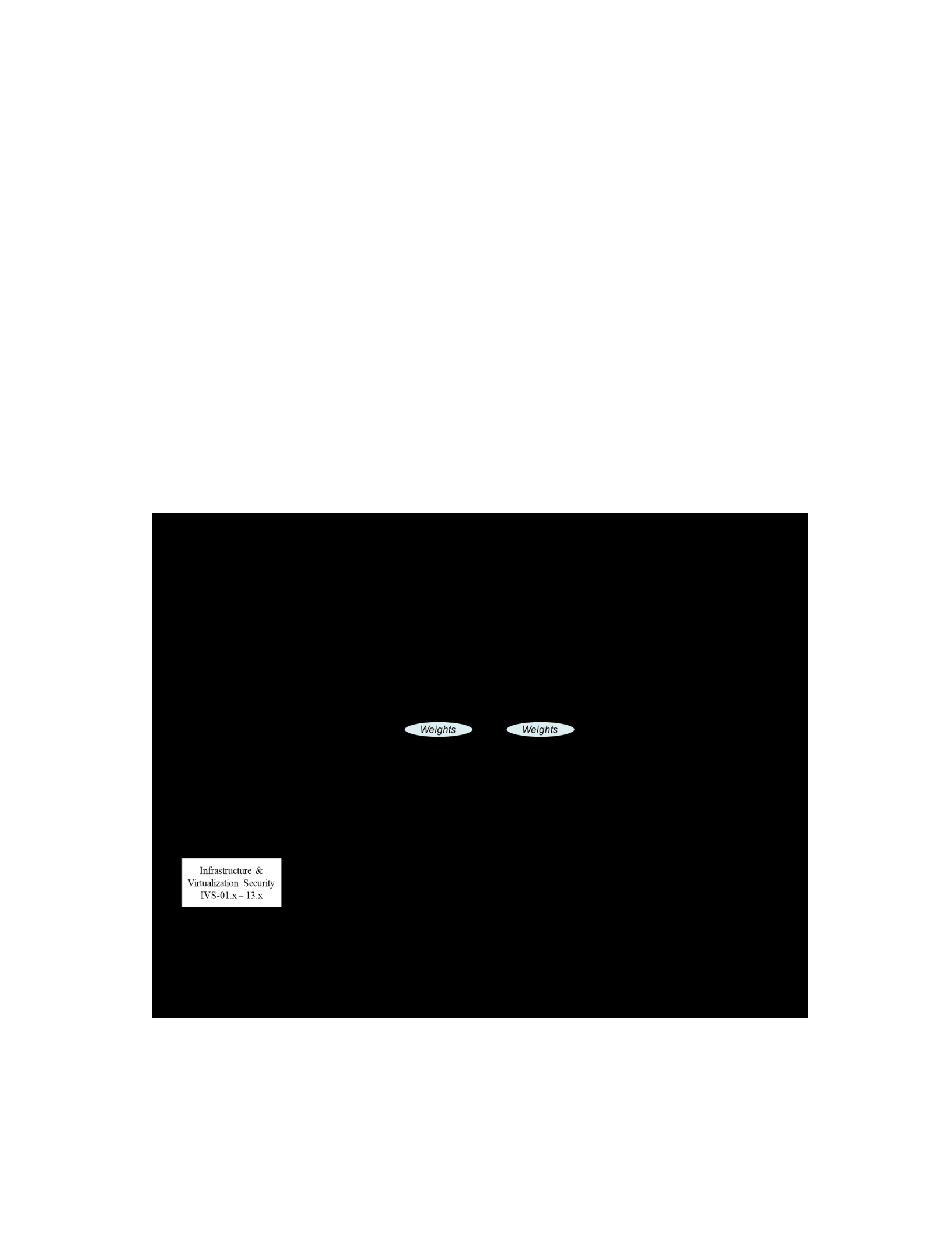
•Level 2 - SLA Content Areas: Identify the high-level criteria, i.e. Content Areas
(e.g. Accessibility), of the SLA structure. The Content Areas represent the
hierarchies of SLA elements and attributes.
•Level 3 - SLA Elements and Attributes (Control Domains, Controls, CAIQs):
Define the CSA CCM Control Domains (e.g. Application & Interface Security)
and related hierarchy of Controls and CAIQs (e.g. AIS-01.x-04.x) within a
Content Area.
•Level 4 – Cloud Service Providers (CSPs): Identify the CSPs (e.g. Amazon,
Google, Microsoft) whose capabilities are being assessed, compared and ranked
with respect to trustworthiness.
Figure 3-3 AHP Hierarchy Structure
58

3.3.2.3.2 Mapping Evaluation Criteria to SLA Structure
Step 2 focuses on mapping evaluation criteria (i.e. CSP CAIQ and Performance) to
the SLA structure defined in Step 1. In Step 2.A. the CSP CAIQ evaluations are scored
(quantified and normalized) based on the degree of CCM compliance for the CSP (i.e.
number of CAIQ questions the CSP answered with a yes). Leveraging the previous Graph
Theory analysis, Appendix D displays the cloud SLA Content Area to CCM Control
Domain mappings and CIAQ compliance (i.e. number and percentage of questions
answered with yes) for each CSP as related to each CCM Control Domain and associated
controls (CSA CAIQ 2017, STAR AWS 2017, STAR Google 2017, STAR Microsoft
2017). The resultant level of CAIQ compliance for each control domain and control as
related to the SLA Content Areas serves as input for the AHP Comparison Matrices. The
weighting of the AHP criterion is based on the quantity of CCM coverage for each SLA
Content Area (i.e. number of CAIQs, Controls and Control Domains as ratios of the totals
associated with each SLA Content Area). For those SLA Content Areas with no direct
CCM mapping (e.g. Accessibility, Termination of Service), the weighting of the criteria is
based on an average quantity of CCM coverage for all SLA Content Area (i.e. average
number of CAIQs, Controls and Control Domains as ratios of the totals associated with
each SLA Content Area). For those CCM Control Domains (e.g. Datacenter Security;
Interoperability & Portability; Mobile Security; Supply Chain Management,
Transparency, and Accountability) that do not map directly to a SLA Content Area, a
group has been created (Capability outside SLA CAs) to represent the AHP related
calculations and analysis for the associated criteria.
In Step 2.B. (similar to Step 2.A.), CSP cloud SLA Content Areas with non-CAIQ
criteria are quantified, normalized and weighted. For SLA Content Area Availability, CSP
59

performance is measured and used for the calculations. Table M-1 displays CSP Compute
Service Availability performance using data recorded in Table M-2 and originating from
Gartner’s Technology Planner Cloud Module (Gartner 2017). The measurements for each
CSP spans between 2015 and 2017 and are normalized and weighted based on the number
of service regions in operation during each measurement period. The total and weighted
service region availability for each CSP during each measurement period is calculated
based on the actual service region measurements (Table M-2) for each CSP (Gartner
2017). Missing measurement data in Table M-2 cells represent service regions that are
either not yet in service for the specified measurement period, or lack measurement data
for the full measurement period. Similar to Step 2.A. and CCM compliance for each CSP
(via CAIQ), the availability performance for each CSP is a proportion (based on
measurements and number of service regions) associated with the SLA Content Area (i.e.
AHP evaluation criterion) Availability.
3.3.2.3.3 Comparison Matrices – SLA Content Areas and CSPs
Step 3 focused on pairwise comparisons and building AHP comparison matrices. Two
types of comparison matrices (using terms outlined in Table 3-1) were constructed:
•Comparison Matrix for SLA Content Area capability criteria. This matrix
represents pairwise comparisons of the AHP evaluation criteria utilizing SLA
Content Area capability ratios calculated by Step 2.
•CSP Comparison Matrices for SLA Content Areas. These matrices (one for each
SLA Content Area) represent pairwise comparisons utilizing CSP capability
ratios for each SLA Content Area calculated by Step 2.
60
Table 3-1 AHP Comparison Matrices and Priority Vector Terms
Term Definition
ca SLA Content Area.
Ci CSP i where i=a for Amazon, i=g for Google, i=m for Microsoft.
Wca Weight factor for SLA Content Area criteria (ca).
Vi,ca Value of content area (ca) capability ratio score for CSP (Ci).
Ri/j,ca Relative rank ratio for pairwise comparison Vi,ca / Vj,ca for two CSPs (Ci and
Cj).
Ci / Cj Relative rank (Ri/j,ca) of Ci over Cj regarding ca.
PVca Priority vector entry for SLA Content Area (ca).
PV Ci Priority vector for CSP (Ci).
WPV Ci Weighted priority vector for CSP (Ci).
TL Ci Trustworthiness level for CSP (Ci).
When performing the pairwise comparisons in each SLA Content Area comparison
matrix, the relationship of CSP capability ratio scores between two CSPs was represented
as: Vi,ca / Vj,ca (for CSPs Ci and Cj). The result of the above pairwise comparison
calculation was the relative rank ratio (Ri/j,ca), which indicated the performance of Ci
compared to Cj, for the specified SLA Content Area (ca). For each SLA Content Area, the
comparison matrix (size 3 x 3 based on a pairwise comparisons of Amazon, Google,
Microsoft) would be constructed as shown in equation 3.1 (SLA Content Area
Comparison Matrix structure):
(3.1)
3.3.2.3.4 SLA Content
Area Reciprocal Matrices
and Priority Vectors
Step 4 creates the normalized, reciprocal matrices and priority vectors (i.e.
61
CaCgCm
Ca(Ca / C a ) (Ca / C g ) (Ca / C m )
CM ca
=
Cg(Cg / C a ) (Cg / C g ) (Cg / C m )
Cm(Cm / C a ) (Cm / C g ) (Cm / C m )

normalized principle Eigenvector) for the AHP evaluation criteria (i.e. SLA Content Area
capability) and for the CSP capability per each SLA Content Area. Two types of priority vectors
have been constructed..
•Priority Vector for SLA Content Area capability (AHP evaluation criteria). This
priority vector is related to the comparison matrix calculated in Step 3. The
priority vector represents the weights in Table 3-2 for each SLA Content Area
used to calculate the overall CSP priority vectors.
•CSP Priority Vectors for each SLA Content Area. These priority vectors (one for
each SLA Content Area) are related to the comparison matrices for each SLA
Content Area calculated in Step 3. The priority vectors were used as input to Step
5 for performing CSP AHP based estimation to calculate the overall CSP priority
vectors.
Utilizing Equation 3.2 (Normalized, reciprocal SLA Content Area Matrix and Priority
Vector), the following steps (using the terms in Table 3-1) were taken when building the
normalized, reciprocal matrices and priority vectors. Using the SLA Content Area
Comparison Matrix from Equation 3.1 (SLA Content Area Comparison Matrix structure),
the columns were summed, then each element (Ci / Cj) was divided by the sum of its
column (Ri/j,ca / ∑-+.,0,$ Ri/j,ca) to normalize the relative weight of each element.
CaCgCmPVca =
Ca(Ca / C a ) / sum (Ca / C g ) / sum (Ca / C m ) / sum ∑ (C a / C j) / 3 (j=a,g,m)
Cg(Cg / C a ) / sum (Cg / C g ) / sum (Cg / C m ) / sum ∑ (C g / C j) / 3 (j=a,g,m)
Cm(Cm / C a ) / sum (Cm / C g ) / sum (Cm / C m ) / sum ∑ (C m / C j) / 3 (j=a,g,m)
su
m
∑ C i / C a∑ C i / C g∑ C i / C m
(i=a,g,m) (i=a,g,m) (i=a,g,m)
(3.2)
Once each matrix element is normalized, the priority vectors PV (i.e. normalized
principle Eigenvectors) were created by averaging each row of the normalized, reciprocal
matrix for each SLA Content Area (∑1+.,0,$ Ri/j,ca / 3). The sum of all elements in the
62

priority vector for each SLA Content Area is one. The priority vector (PV) in Equation
3.2 (Normalized, reciprocal SLA Content Area Matrix and Priority Vector) represents
relative weights related to each CSP for each SLA Content Area. The priority vector
represents numerical values that specify the CSP order of preference for the SLA Content
Area (i.e. a representation of which CSP is more capable for each SLA Content Area).
3.3.2.3.5 CSP Priority Vectors and Final Trustworthiness
The final phase (Step 5) calculates the AHP based estimation by building the CSP
priority vectors based on the Step 4 SLA Content Area Priority Vectors. The weighted
factors (Table 3-2) calculated by Step 4 are then applied to the CSP priority vectors to
build the weighted CSP priority vectors. Finally, the Trustworthiness Level for each CSP
is calculated by aggregating the weighted CSP Priority Vectors. The AHP based
estimations (i.e. CSP Priority Vectors and weighting factors, weighted CSP Priority
Vectors) and Trustworthiness Levels for each CSP are introduced in Chapter 4 – Results.
The following steps (using the terms in Table 3-1) were taken when building the CSP
Priority Vectors, applying the weighting and calculating CSP Trustworthiness Levels. The
SLA Content Area priority vectors (PVca) introduced by Equation 3.2 (Normalized,
reciprocal SLA Content Area Matrix and Priority Vector) are arranged by CSP to build
CSP priority vectors as defined by Equation 3.3 (AHP Based Estimation – CSP Priority
Vector). Refer to Table 3-2 for ca abbreviations.
PV C i = ( PV ca … PV ca )
(i=a,g,m)
(ca = Acc, ACA, Avail, Chg Man, CS Perf, CS Supp, Data Man, Gov, Info Sec, Pro PII, Svc Rel, Term Svc, Outside CA)
(3.3)
For each CSP Priority Vector (PV Ci) per Equation 3.3 (AHP Based Estimation – CSP
Priority Vector), each SLA Content Area priority vector entry (PVca) was multiplied by
63

corresponding SLA content area criteria weight (Table 3-2). The result is weighted AHP
based estimation for each CSP as represented in Equation 3.4 (Weighted AHP Based
Estimation – CSP Priority Vector and Weight Factors), i.e. weighted priority vectors for
each CSP. Refer to Table 3-2 for ca abbreviations.
WPV C i =( PV ca x W ca … PV ca x W ca )
(i=a,g,m)
(ca = Acc, ACA, Avail, Chg Man, CS Perf, CS Supp, Data Man, Gov, Info Sec, Pro PII, Svc Rel, Term Svc, Outside CA)
(3.4)
In Equation 3.4 (Weighted AHP Based Estimation – CSP Priority Vector and Weight
Factors), the weight factor (Wca) was multiplied by each SLA Content Area Priority
Vector (PVca) entry. The calculation of the weight factors (presented in Table 3-2 and
reviewed in Step 4) was based on the priority vector for SLA content area capability
criteria.
Table 3-2 SLA Content Area Criteria Weight for CSP Priority Vectors
Weight SLA Content Area Criteria
0.0655 Acc AccessibilityAttestations,
Certifications and
0.0236 ACA Audits
0.0982 Avail Availability
0.0222 Chg
Man
Change Management
0.0653 CS
Perf
Cloud Service Performance
0.0264 CS
Supp
Cloud Service Support
0.0348 Data
Man
Data Management
0.0473 Gov Governance
0.3198 Info
Sec
Information Security
0.1029 Pro PII Protectionof PII
0.0487 Svc Service Reliability
64

Rel
0.0655 Term
Svc
Termination of
Service
0.0799 Outside
CA
Capability outside SLA CAs
For each CSP (Ci where i=a,g,m), the weighted priority vector entries (PVca x Wca) for all
SLA Content Areas (ca) from Equation 3.4 (Weighted AHP Based Estimation – CSP
Priority Vector and Weight Factors), and WPV Ci, were aggregated to represent the final
CSP Trustworthiness Level represented by Equation 3.5 (CSP Trustworthiness Level).
TL C i = ∑ ( PV ca x W ca ) (3.5)
3.3.3 Linear Regression to Model and Predict Cloud SLA Availability
Linear regression analysis was used to investigate functional relationships between
cloud service provider (CSP) and cloud compute service variables and ultimately develop
models to predict cloud compute service availability. The models, analysis and
predictions were in support of the following hypothesis.
Predicting SLA-based cloud service availability has greater accuracy when
calculated with more criteria than just historical cloud service downtime (e.g. CSP
trustworthiness; global cloud service locations, resource capacity and performance).
To analyze and test the stated hypothesis, two linear regression models (simple
variable and multiple variable) were created to relate predictor variables with the
response variable and drive predictions that enable analysis and testing of the stated
hypothesis. This chapter reviews the linear regression methodology was utilized for
building and analyzing the models, and ultimately testing the hypothesis (Chatterjee and
Hadi 2013, Kutner, Nachtsheim and Neter 2008, Harrell 2015).
65

The following high level activities were followed to guide the regression analysis
(Chatterjee and Hadi 2013, Kutner, Nachtsheim and Neter 2008, Harrell 2015).
•Define the problem statement.
Hypothesis: Predicting SLA-based cloud service availability has greater accuracy
when calculated with more criteria than just historical cloud service downtime
(e.g. CSP trustworthiness; global cloud service locations, resource capacity and
performance).
•Select relevant variables that explain or predict the response variable (refer to
Appendix N Table N-1 for description of variables).
Response variable = Y (Cloud service Availability)
Predictor variables = X1, X2, X3, X4, X5 o X1 = Cloud service downtime o
X2 = CSP trust level o X3 = Global service region locations o X4
= Number of cloud service regions within a global location o X5
= Cloud service performance
•Identify and collect required data (refer to section 3.3.3.1 for analysis of data).
Required data for the linear regression analysis was provided by Gartner and
cloud service providers (CSPs) Amazon, Google, Microsoft (Gartner 2017,
CloudHarmony 2017, SLA AWS 2017, SLA Google 2017, SLA Microsoft 2017).
•Define linear regression model specification.
The relationship between the response and predictor variables can be
approximated by the regression models of Equation 3.6 and Equation 3.7.
Y = f(X1) + E for the simple linear regression (3.6)
66

Y = f(X1, X2, X3, X4, X5) + E for the multiple linear regression (3.7)
As previously introduced, response variable Y represents cloud service
availability, and the predictor variables are represented as follows (refer to Table
N-1 for description of variables): o X1 = Cloud service downtime o X2 =
CSP trust level o X3 = Global service region locations o X4 =
Number of cloud service regions within a global location o X5 =
Cloud service performance
“E is assumed to be a random error representing the discrepancy in the
approximation” (Chatterjee and Hadi 2013, Kutner, Nachtsheim and Neter 2008,
Harrell 2015). The error accounts for the “failure of the model to fit the data
exactly” (Chatterjee and Hadi 2013, Kutner, Nachtsheim and Neter 2008, Harrell
2015).
An example linear regression equation (Equation 3.8) for the models is
represented by:
Y = B0 + B1X1 + B2X2 + … + BpXp + E (3.8)
where B0, B1, …, Bp called the “regression coefficients, are unknown constants to
be determined (estimated) from the data” (Chatterjee and Hadi 2013, Kutner,
Nachtsheim and Neter 2008, Harrell 2015).
•Select the fitting method.
The method of least squares was used for estimating the parameters of the model
based on the collected data.
•Fit the model.
Fit the model to the collected data to estimate the regression coefficients using
least squares.
67

•Validate and criticize the model.
Analyze linear regression assumptions for both models and related data, and
validate the Goodness of Fit. Refer to section 3.3.3.6 for details.
•Utilize the model(s) for the solution to the identified problem.
3.3.3.1 Data Analysis
As presented in Appendix O (Table O-1, O-2, O-3), the data from Gartner was
provided from their cloud planning tool (Cloud Decisions) and focuses on Amazon,
Google, Microsoft observations between 2015-2017. In total, 41 global service regions
provided 101 observations related to the 6 variables (response variable, 5 predictor
variables).
The essence of my hypothesis was that the accuracy of predicting future cloud
computing service availability improved when leveraging multiple predictor variables vs
a single predictor (i.e. historical downtime). The variables for the regression analysis
(both simple and multiple variable) are presented in Table N-1.
For linear regression analysis, RStudio Version 1.0.136, an integrated development
environment for statistical computing and graphics, was used. The data was randomly
split using the R function sample() with 85% used for training the model and 15% used
for testing predictions with model. Refer to Appendix A for the complete dataset and to
Appendix O for additional details concerning the datasets used to train and test the simple
and multiple linear regression analysis models.
3.3.3.2 Simple Regression Model
The simple linear regression model is denoted by the equation Y=B0 + B1X + E where
B0 and B1 represent the regression coefficients and E is the “random disturbance or error”
(Chatterjee and Hadi 2013, Kutner, Nachtsheim and Neter 2008). Y (cloud compute
68

service Availability) is “approximately a linear function” of X (cloud compute service
Downtime) and E measures the “discrepancy in the approximation” (Chatterjee and Hadi
2013, Kutner, Nachtsheim and Neter 2008). B1 is the slope (i.e. changes in Availability
for a unit of change in Downtime), and B0 is the constant coefficient (i.e. intercept,
predicted value of Y when X = 0). For the model, the goal is to estimate parameters B0
and B1 and “find the straight line that provided the best fit” of the response versus
predictor variable using least squares method (Chatterjee and Hadi 2013, Kutner,
Nachtsheim and Neter 2008). An initial model fitting was performed followed by analysis
of the results and regression assumptions. Outliers were then assessed, predictor variable
were transformed, and the final model was again fitted and then analyzed.
After analysis of initial linear regression model, assumptions (including outliers),
variable scatterplot (Availability, Downtime) and relationships were assessed. A K-fold
cross-validation method was applied to calculate measure of errors for polynomial fit
with different degrees. The cross-validation analysis was then leveraged to build the
modified simple linear regression model for a better fit.
3.3.3.3 Multiple Regression Model
The multiple linear regression model is denoted by the equation Y=B0 + B1X1 + B2X2
+ B3X3 + B4X4 + B5X5 + E, where B0, B1, B2, B3, B4, B5 are the regression coefficients,
and E is the “random disturbance or error” (Chatterjee and Hadi 2013, Kutner,
Nachtsheim and Neter 2008). Y (cloud compute service Availability) is “approximately a
linear function” of X1 (cloud compute service Downtime), X2 (cloud service provider
Trust level), X3 (Location of cloud compute service region), X4 (number of cloud
compute service Regions), X5 (cloud compute service Performance) and E measures the
“discrepancy in the approximation” (Chatterjee and Hadi 2013, Kutner, Nachtsheim and
69

Neter 2008). Each regression coefficient (B1, B2, B3, B4, B5) represents the slope (i.e.
changes in Availability for a unit of change in a coefficient as other coefficients are held
constant), and B0 is the constant coefficient (i.e. intercept, predicted value of Y when X =
0). For the model, the goal was to estimate parameters B0, B1, B2, B3, B4, B5 and “find the
straight line that provided the best fit” of the response versus predictor variables using
least squares method (Chatterjee and Hadi 2013, Kutner, Nachtsheim and Neter 2008).
An initial model fitting was performed followed by analysis of the results and regression
assumptions. Outliers were then removed, predictor variables were transformed, and the
final model was again fitted and then analyzed.
After analysis of initial linear regression model, assumptions (including outliers),
variable matrix scatterplot and relationships, multiple methods were applied to selecting a
subset of predictor variables for the multiple regression equation. The methods included
stepwise selection (forward, backward, both using AIC), all-subset regression using
leaps, and lastly best subset selection.
3.3.3.4 Regression Model Summary
From the model summary output and the variable scatterplot the following analysis
occurred.
•Is the p-value for the overall model < 0.05 (an overall test of the statistical
significance for the model)?
•Does the model have a strong R-squared measure, indicating that majority of
variance related to the response variable is explained by the predictor variable(s)?
The closer the R-squared value is to 1, the better the model explains the variance.
70

•How large was the residual standard error, which measures the average amount
the response variable “deviates from the true regression line for any given point”
(i.e. how far observed Y values are from the predicted values) (Tattar, Ramaiah,
and Manjunath 2016, Chatterjee and Hadi 2013)?
•Are the p-values for the regression coefficients statistically significant (i.e. <
0.05)?
•After analysis and interpretation of the model’s results, ANOVA and linear
regression assumptions were analyzed, driving any required variable
transformation (Tattar, Ramaiah, and Manjunath 2016, Chatterjee and Hadi
2013).
3.3.3.5 ANOVA of Regression Model
Analyze the ANOVA results for the model. Check the ANOVA F-test results (i.e. Ftest
statistic and p-value) to confirm linear relationship between the response variable and
predictor variable(s). Also check the regression sum of squares to conclude whether most
of the variation related to the observed response variable data points were attributed to the
predictor variable(s) vs “random error” (Tattar, Ramaiah, and Manjunath 2016).
3.3.3.6 Regression Assumptions
To further assess the linear regression model and the relationship between Availability
and predictor variable(s), a number of required assumptions (as previously introduced in
the Methodology chapter) were examined. Related measures and linear regression
diagnostics were organized based on the assumptions being analyzed. The assumptions
include Linearity, Normality, Independence, Homoscedasticity, and Outliers
(Fox 1991, Chatterjee and Hadi 2013, Tattar, Ramaiah, and Manjunath 2016).
71

3.3.3.6.1 Linearity
The analysis related to this assumption looks for a linear association between the
explanatory variable(s) and response variable Availability. As part of the analysis, the
following R related functions were utilized for both simple and multiple linear regression
models (Fox 1991, Chatterjee and Hadi 2013, Tattar, Ramaiah, and Manjunath 2016).
The regression diagnostic plots (Equation 3.9 Residuals vs Fitted, Equation 3.10
Scale-Location) were assessed for linear relationships between response variable and
predictor variable(s). The analysis looked for a flat (horizontal) red line on plots with
ideally, no data point pattern.
R: plot(RegressionModel, which=1) (3.9)
R: plot(RegressionModel, which=3) (3.10)
Checked ANOVA F-test results using Equation 3.11 to confirm a linear relationship
between response variable and predictor variable(s).
R: anova() (3.11)
Used Equation 3.12 to check if the mean of the residuals were close to zero indicating a
linear association existed.
R: mean() (3.12)
3.3.3.6.2 Normality
The analysis related to this assumption looked for a normal distribution of residuals.
As part of the analysis, the following R related functions were utilized for both simple
and multiple linear regression models (Fox 1991, Chatterjee and Hadi 2013, Tattar,
Ramaiah, and Manjunath 2016).
A histogram was plotted using R: rstandard(RegressionModel).
72

The regression diagnostic plot (Equation 3.13 Q-Q) was assessed, looking for
observations roughly aligned with the diagonal line of residuals.
R: plot(RegressionModel, col="blue", which=2) (3.13)
Skewness Equation 3.14 (ideally = 0) and kurtosis Equation 3.15 (ideally = 3) of the
models were assessed for normal distribution (Schafer 2000, Kutner, Nachtsheim and
Neter 2008, Fox 1991).
R: skewness() (3.14)
R: kurtosis() (3.15)
3.3.3.6.3 Independence
The analysis related to this assumption looked for independence by assessing if
correlation / auto-correlation existed between observations. As part of the analysis, the
following R related functions were utilized as expressed below by R:.
The auto-correlation function (Equation 3.16 acf) plot was analyzed for observation
dependencies.
R: acf() (3.16)
For simple linear regression:
Correlation (Equation 3.17) was tested. If p-value was >= 0.05 then no correlation existed
(Chatterjee and Hadi 2013).
R: cor.test() (3.17)
Variance (Equation 3.18) in predictor variable was assessed. If the result was significantly
larger than 0 then independence was satisfied.
R: var() (3.18)
For multiple linear regression:
73

Correlation of variables (Equation 3.19) was analyzed (Chatterjee and Hadi 2013).
R: corrplot() (3.19)
Variance inflation factors (Equation 3.20) for multicollinearity were analyzed (should be
< 4 for each predictor variable).
R: vif() (3.20)
3.3.3.6.4 Homoscedasticity
The analysis related to this assumption looked at homoscedasticity and variability of
residuals utilizing the following R plots.
Regression diagnostic plots (Equation 3.21 Residuals vs Fitted, Equation 3.22
ScaleLocation) were analyzed for homoscedasticity. With homoscedasticity (equal
variances) of residuals, the red line on the plots should be approximately flat (horizontal)
with little to no pattern present (i.e. the data points are cloud like) (Fox 1991, Chatterjee
and Hadi 2013, Tattar, Ramaiah, and Manjunath 2016).
R: plot(RegressionModel, which=1) (3.21)
R: plot(RegressionModel, which=3) (3.22)
3.3.3.6.5 Outliers
The analysis related to this assumption utilized the following R plots to analyze
outliers, leverage and extreme values on variables relative to other observations.
Regression diagnostic plots (Equation 3.23 Cook’s distance, Equation 3.24 Residuals
vs Leverage) for outliers, influential observations and leverage were analyzed. Rule of
thumb is no Cook’s distance > 1, and standardized residuals should be near 0 and within
2-3 standard deviations from 0. Ideally, the solid red line should be flat (horizontal) and
74

close to the mid-dashed line with no large Cook’s distance > 0.5 (Fox 1991, Chatterjee
and Hadi 2013, Tattar, Ramaiah, and Manjunath 2016).
R: plot(RegressionModel, which=4) (3.23)
R: plot(RegressionModel, which=5) (3.24)
Influential data points, outliers and leverage were identified and analyzed using
Equations 3.25 and 3.26.
R: ols_rsdlev_plot(Model) (3.25)
R: ols_dffits_plot(Model) (3.26)
3.3.3.7 Linear Regression based Predictions
The predictions related to the simple and multiple linear regression models leveraged
the following R related functions (Equation 3.27, 3.28) as expressed below by R:.
R: predict(SimpleModel, newdata = SimpleTestData) (3.27)
R: predict(MultipleModel, newdata = MultipleTestData) (3.28)
Predictions were calculated based on both linear regression models (simple and
multiple). Predicted availability vs observed comparisons were plotted (with 95%
confidence interval and prediction interval) for both simple and multiple linear
regression. The fit of the models were compared and contrasted. While the confidence
interval illustrates something about the estimated parameters, the prediction interval
illustrates where the next future observation is likely to fall (given a “tolerance level”
such as 95%) (Chatterjee and Hadi 2013, Kutner, Nachtsheim and Neter 2008).
3.3.3.8 Comparing Linear Regression Models (Simple vs Multiple)
The model comparison and analysis looked at how the predictor values between the
two models effected availability %. The model testing used real operational data for cloud
compute services. All data was either provided directly from the cloud service providers
75

and/or validated against published cloud service provider data (e.g. CSP outage
notifications and duration were cross-checked against the Gartner live monitoring and
performance data).
3.3.3.8.1 Goodness of Fit Measures and Validating the Models
Goodness of Fit measures for both simple and multiple linear regression models were
calculated and analyzed using the R functions presented in Appendix F (Tattar, Ramaiah,
and Manjunath 2016, Chatterjee and Hadi 2013, Harrell 2015). Predictions for both
models were performed with multiple prediction intervals between 50% and 95% using
5% increments. The total and average number of successful predictions that fell within
the prediction intervals were assessed for both models. ANOVA was used to compare the
models and measure what the multiple linear regression adds to the linear prediction
above and beyond the simple linear regression model. The following R ANOVA function
(Equation 3.29) as expressed by R: was utilized.
R: anova(SimpleModel, MultModel) (3.29)
3.3.3.9 Hypothesis Testing
The hypothesis asserts:
Predicting SLA-based cloud service availability has greater accuracy when
calculated with more criteria than just historical cloud service downtime (e.g. CSP
trustworthiness; global cloud service locations, resource capacity and performance).
Testing of the hypothesis assessed whether the additional regression coefficients of
the multiple linear regression model provided statistically significant contribution to
explaining cloud service availability vs the simple linear regression model with a single
coefficient. That is, did the additional variables of the multiple linear regression model
provide explanatory or predictive power to the model?
76

The following null and alternative hypothesis were defined for testing:
H0 : Multiple = Simple LR model, i.e. zero difference in accuracy (Bj = 0); no
additional variables have explanatory/predictive power (don’t contribute to the
Simple LR model).
Ha : At least one additional variable (Bj) has a statistically significant contribution
to explaining/predicting Y (Bj != 0), and therefore should remain in the model.
Decision to reject or fail to reject the null hypothesis was based on the Goodness of
Fit measures, including the ANOVA F-test results comparing the two models, and the
validation results concerning successful predictions.
77

Chapter 4. Results
A comprehensive study of the cloud service level agreement (SLA) lifecycle was
conducted, analyzing cloud SLA and cloud security specifications and frameworks, cloud
service provider (CSPs) trustworthiness, historical cloud service performance and
benchmarks (e.g. cloud IT resources, CSP SLAs). The analysis focused on the top three
CSPs (Amazon, Google, Microsoft) and how the aforementioned data influenced cloud
service performance and the ability to predict cloud SLA Availability. My approach for
predicting cloud SLA performance and hypothesis testing was based on the composite
outcomes of the following methodologies: Graph Theory, Analytic Hierarchy Process,
Linear Regression Analysis. The output of Graph Theory analysis served as input to
Analytic Hierarchy Process, which then produced output that served as input to the Linear
Regression predictive models. Refer to Figure 3-1 Methodology Map for additional
details regarding the source and flow of data and relationships between the
methodologies. The data and sources reviewed in Chapter 3 (Methodology) for each
methodology consisted of:
•Graph Theory o Cloud SLA standards from ISO/IEC, EC, ENISA
(ISO/IEC 2016, EC 2014, Hogben, Giles and Dekker 2012).
oCloud security framework (CCM, CAIQ) from CSA (CSA CCM 2017, CSA
CAIQ 2017).
oCSP SLAs from Amazon, Google, Microsoft (SLA AWS 2017, SLA Google
2017, SLA Microsoft 2017).
oCSP cloud security assessments (CSP CAIQ) from CSA STAR (STAR AWS
2017, STAR Google 2017, STAR Microsoft 2017, CSA STAR).
78

•Analytic Hierarchy Process o CSP cloud SLA and security model and
analysis from Graph Theory for Amazon, Google and Microsoft.
oCSP historical SLA performance from Gartner’s Technology Planner Cloud
Module tool renamed Cloud Decisions (Gartner 2017).
•Linear Regression Analysis o CSP trustworthiness level and quantified CSP
cloud SLA from Analytic Hierarchy Process for Amazon, Google and
Microsoft.
oCSP historical cloud service performance and benchmarks from Gartner’s
Technology Planner Cloud Module tool (Gartner 2017). Historical data
included CSP SLA performance, network performance and resource
utilization.
The predictive modeling and analysis results ultimately were used to test the
hypothesis:
Predicting SLA-based cloud service availability has greater accuracy when
calculated with more criteria than just historical cloud service downtime (e.g. CSP
trustworthiness; global cloud service locations, resource capacity and performance). The
primary question to be answered: Does predicting cloud computing SLA performance
have a greater accuracy when calculated with historical SLA performance, cloud service
performance, and CSP trustworthiness, rather than just historical cloud service downtime?
4.1 Graph Theory to Model Cloud SLAs and Security Controls
As outlined in Chapter 3 (Methodology), industry SLA standards (ISO/IEC 2016,
NIST 2015, EC 2014), industry cloud security controls (CSA CCM 2017), cloud security
controls and SLAs for CSPs (e.g. Amazon, Google, Microsoft) (STAR AWS 2017,
79

STAR Google 2017, STAR Microsoft 2017, SLA AWS 2017, SLA Google 2017, SLA
Microsoft 2017) were analyzed using Graph Theory (Roberts 1978). A number of
questions were introduced that drove the identification and development of the graphs.
The questions and answers are addressed below with their corresponding graph(s).
Chapter 3 (Methodology) introduced NetDraw (Borgatti 2002), the network analysis
software package that was used for visualizing the industry and CSP cloud SLA and
security capabilities. Each subsection below reviews corresponding graphs and NetDraw
configuration along with observations related to the graphical depiction of the data
(nodes) and strength of the data relationships (ties … lines). The size of the node and
thickness of the line indicates the strength of the node and relationship based on the
criteria described for each graph.
For each graph, the shape and color of the node depicts the type of data (e.g. type of
organization, SLA or security capability). The organizations are comprised of CSPs which
are represented by circle nodes (Amazon=orange, Google=yellow,
Microsoft=blue) and industry standards bodies represented by triangle nodes (CSA=cyan,
EC=red, ENISA=pink, ISO/IEC=green).
The SLA related actors (square nodes) represent CSP SLAs for Amazon, Google and
Microsoft (same CSP colors for unique SLAs, and color teal for common SLAs), and
industry cloud SLA standards representing content areas (brown nodes) for EC, ENISA
and ISO/IEC. The security related actors (square nodes) represent security control
domains (maroon nodes) for CSA CCM. As previously discussed, the relationships and
strengths of industry cloud SLA standards and security capabilities influence the
trustworthiness level of the CSP.
80

For each graph (Figures 4-1 to 4-6), observations are provided along with an
assessment of the graph according to the following factors (Satyanarayana, Bhavanari and
Prasad 2014, Diestel 2005):
•Degree centrality – I’m assessing the number of neighbors each node has (i.e. ties
directed to each node (indegree) and number of ties each node directs to others
(outdegree)). The insight related to organization nodes (especially those with
greater degree centrality numbers) reflects their level of influence and alignment
to SLA content areas and security control domains. For SLA and security control
nodes, the insight relates to the relevance of the SLA content area or security
control domain to the industry and organizations.
•Betweeness centrality – For each vertex (node), betweeness looks at the number
of shortest paths that pass through the vertex (i.e. for each vertices pair, look at
number of shortest path with minimum number of edges). The measure quantifies
the control a node has on two other nodes. For the analysis of the graphs, the
insight I’m assessing is not how well connected a node is but rather how
dependent other nodes are on the node being measured. This considers the impact
to others nodes when removing the node being measured. For organization nodes,
removal could reduce the strength and value of an SLA content area and/or
security control domain. For SLA and security control nodes, the removal could
reduce the SLA and/or security capability of an organization.
4.1.1 Overview of Cloud SLA Standards, Standards Organizations and CSPs
Based on the analysis and findings related to the produced graphs, Table 4-1 was
created to show how the organizations (standards bodies CSA, EC, ENISA, ISO/IEC; and
81
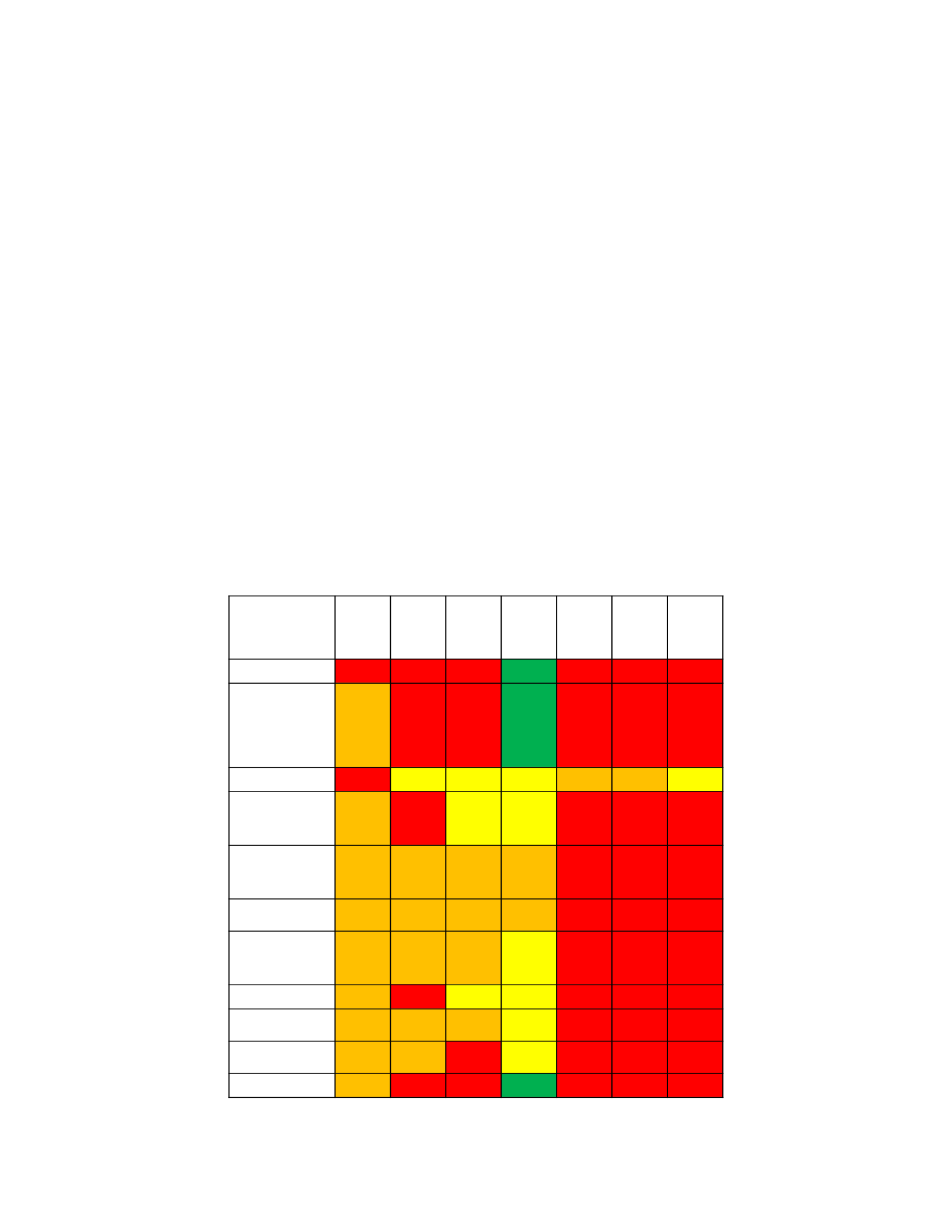
CSPs Amazon, Google, Microsoft) contributed to the cloud industry SLA standards
content areas, and compared with each other’s contribution. The content areas are a result
of the Graph Theory model for cloud SLA standards based on industry standard bodies
(ISO/IEC 2016, EC 2014, Hogben, Giles and Dekker 2012).
Table 4-1 identifies the extent to which each organization contributes to a content area
with respect to the total contributions from all organizations for that content area. Green
indicates the organization contributes and aligns with 100% of the content area SLA
capabilities. Yellow indicates partial contribution and alignment has been achieved with
between 50-99% of the content area SLA capabilities. Orange indicates partial
contribution and alignment with between 1-49% of the content area SLA capabilities. Red
indicates none of the content area SLA capabilities were addressed by the organization.
Table 4-1 Comparison of Cloud SLA Standards by Standards Organizations and CSPs
Cloud Industry
SLA
Standards
CSA EC ENISA ISO Amazon Google Microsoft
Accessibility
Attestations,
Certifications
and
Audits
Availability
Change
Management
Cloud Service
Performance
Cloud Service
Support
Data
Management
Governance
Information
Security
Protection of
PII
Service
82
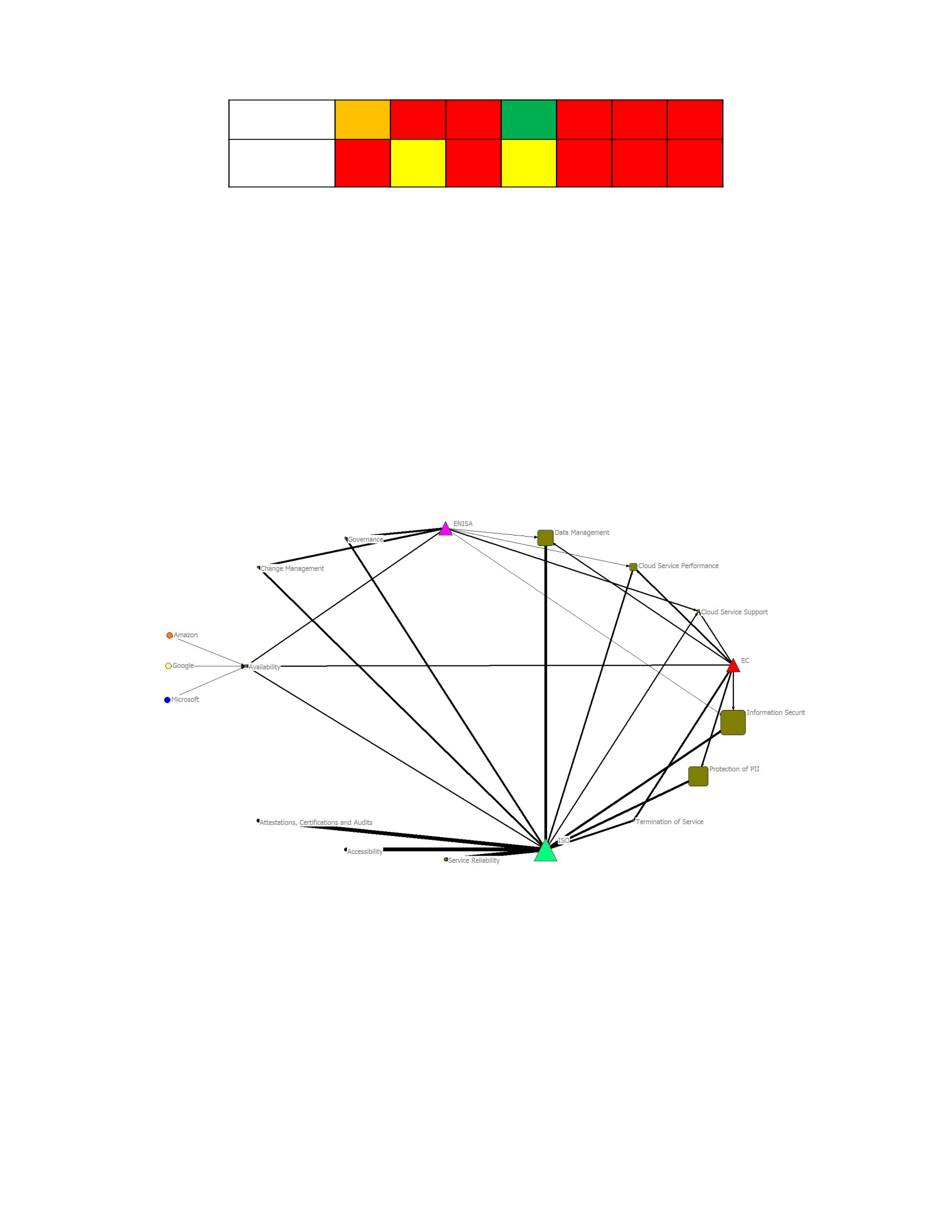
Reliability
Termination
of
Service
4.1.2 Cloud SLA Standards and Organizations
The following question drove the modeling and analysis of Figure 4-1. What cloud
SLA standards are related to what industry standards organizations and CSPs?
Figure 4-1 depicts the contributed work related to cloud SLA standards from
standards bodies (triangle node) ISO/IEC, ENISA and EC (ISO/IEC 2016, Hogben, Giles
and Dekker 2012, EC 2014) in addition to how the work relates with SLAs from CSPs
(circle node) Amazon, Google and Microsoft.
Figure 4-1 Relationships between Cloud SLA Standards and Organizations
The standardized cloud SLA content has been organized into 12 content areas (square
brown node) based on the SLA framework developed by ISO/IEC (ISO/IEC 19086-1
2016, ISO/IEC 19086-2 2017, ISO/IEC 19086-3 2017). For each content area, the node
size is based on the number of cloud SLA details (i.e. components) specific to that content
area in proportion to the combined total number of cloud SLA details (i.e. components)
83

for all content areas. The size of the node for each standards body is based on the number
of relationships across all cloud SLA content areas in proportion to the total number of
available cloud SLA content areas. The thickness (strength) of the relationship (tie)
between a standards body (e.g. EC, ENISA, ISO/IEC) and a specific content area denotes
the quantity of cloud SLA details (i.e. components) the standards body contributed to the
content area in proportion to the total number of cloud SLA details that exist for that
content area.
Based on nodes, ties and relationships modeled in Figure 4-1, Centrality factors were
assessed and the following observations were made (Diestel 2005). Refer to Appendix I
for Degree Centrality details regarding organizations and cloud SLA content areas.
•1 of 12 cloud SLA content areas had a relationship with 3 of 3 CSPs (Amazon,
Google, Microsoft): Availability.
•3 of the 12 cloud SLA content areas received the most contributions (each
represented > 20% of the total components vs the others which were <= 10%):
Information Security, Protection of PII, Data Management.
•ISO/IEC contributed to 12 of 12 cloud SLA content areas; Primary contributor for
9 of 12 (each contribution >= 50% of the content areas’ components):
Accessibility; Attestations, Certifications and Audits; Change Management; Data
Management; Governance; Information Security; Protection of PII; Service
Reliability; Termination of Service.
•ENISA contributed to 7 of 12 cloud SLA content areas; Primary contributor for 2
of 12 (each contribution >= 50% of the content areas’ components): Change
Management, Governance.
84
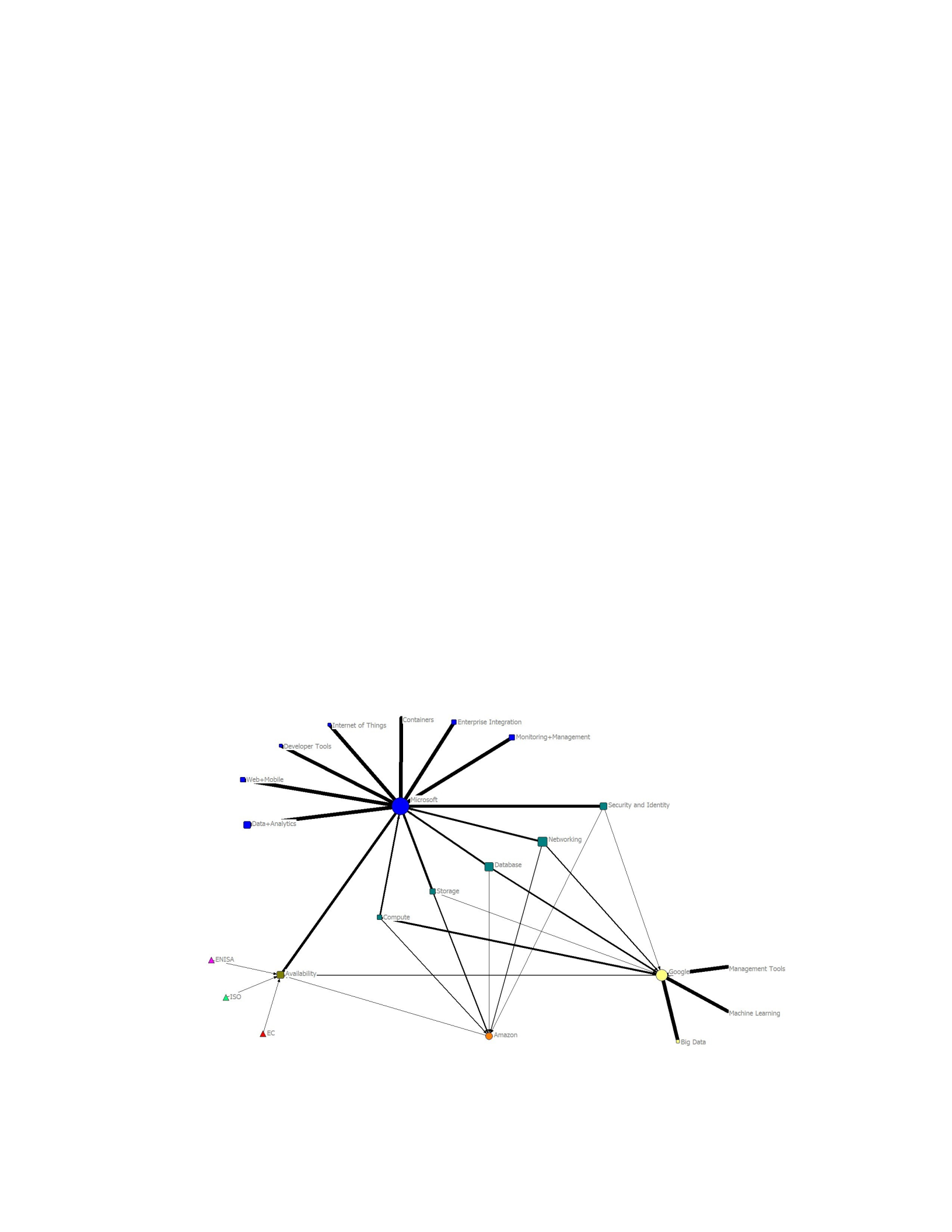
•EC contributed to 7 of 12 cloud SLA content areas; Primary contributor for 1 of
12 (contribution >= 50% of the content areas’ components): Termination of
Service.
4.1.3 CSP SLAs and Cloud SLA Standards
The following questions drove the modeling and analysis of Figure 4-2.
•What SLAs exist for each CSP?
•What SLAs have interrelationships across CSPs and what are the SLA gaps and
overlaps between the CSPs?
•What are the relationships between the CSP SLAs (Amazon, Google, Microsoft),
industry standards organizations (ISO/IEC, EC, ENISA) and industry cloud SLA
standards (i.e. content areas)?
Figure 4-2 depicts the cloud SLAs offered by CSPs (circle node) Amazon, Google
and Microsoft (SLA AWS 2017, SLA Google 2017, SLA Microsoft 2017) and their
relationship cloud SLA standards and standards bodies (i.e. ISO/IEC, EC, ENISA).
85

Figure 4-2 Relationships between CSP SLAs and Cloud SLA Standards
Each CSP offers SLAs that only focus on the Availability industry content area
(brown square node) with respect to the cloud SLA standards (ISO/IEC 2016, Hogben,
Giles and Dekker 2012, EC 2014) from the industry bodies ISO/IEC, EC, ENISA
(triangle node). As depicted by Figure 4-2, all three CSPs offer multiple types of
Availability SLAs that are common (square node teal color), whereas Google and
Microsoft also offer multiple types of Availability SLAs that are unique (square node
color of CSP). For each type (square node) of Availability SLA (common or unique), the
node size is based on the number of underlying cloud service SLAs related to that type in
proportion to the combined total number of underlying cloud service SLAs for all types.
The size of the node for each CSP is based on the number of relationships with different
SLA types (square nodes) and related underlying cloud service SLAs in proportion to the
total number of available SLA types and related total number of underlying cloud service
SLAs across all CSPs. The thickness (strength) of the relationship (tie) between a CSP
(e.g. Amazon, Google, Microsoft) and the Availability industry content area denotes the
quantity of all Availability related SLA types and related underlying cloud service SLAs
for that CSP in proportion to the total number of Availability related SLA types and
related underlying cloud service SLAs for all CSPs. The thickness (strength) of the
relationship (tie) between a CSP and Availability related SLA type (e.g. Compute)
denotes the quantity of underlying cloud service SLAs for that specific SLA type and
specific CSP in proportion to the total number of underlying cloud service SLAs for that
specific SLA type across all CSPs.
86

Based on nodes, ties and relationships modeled in Figure 4-2, Centrality factors were
assessed and the following observations were made (Diestel 2005). Refer to Appendix I
for Degree Centrality details regarding organizations and CSP SLA content areas.
•3 of 3 CSPs (Amazon, Google, Microsoft) have a relationship with 1 of 12 cloud
SLA content areas: Availability.
•15 of 15 CSP cloud SLA types (i.e. 100% of the 84 CSP cloud service SLAs) are
focused on a single cloud SLA content area: Availability.
•4 of the 15 CSP cloud SLA types account for the majority of the CSP cloud
service SLAs (each represented >= 10% of the total CSP cloud service SLAs vs
the others which ranged between 1% to 8%): Data+Analytics, Database,
Networking, Security and Identity.
•5 of the 15 CSP cloud SLA types (representing 50% of the 84 CSP cloud service
SLAs) are common among 3 of 3 CSPs (Amazon, Google, Microsoft): Compute,
Storage, Database, Networking, Security and Identity.
•Of the remaining 10 of the 15 CSP cloud SLA types related to unique cloud
service SLAs, Microsoft provides 70% and Google 30%.
•Of the total CSP cloud service SLAs, Microsoft provides > 70%, of which 40%
were common to all CSPs (Microsoft accounted for >= 50% of 4 of the 5 common
cloud service SLAs: Storage, Database, Networking, Security and Identity).
4.1.4 CSA CCM and Cloud SLA Standards
The following questions drove the modeling and analysis of Figure 4-3. Knowing the
CCM control domains have some overlap with the SLA standards, what is the
87
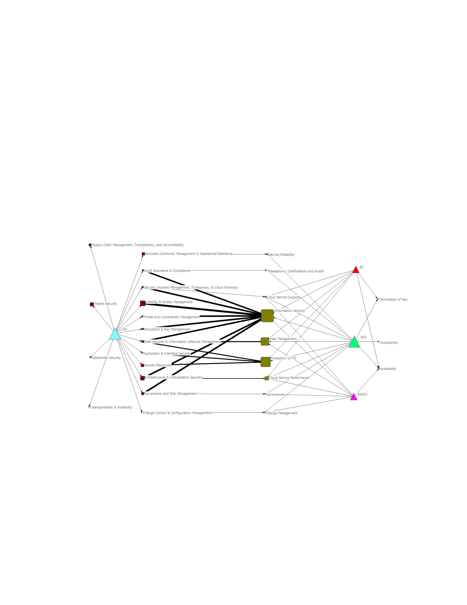
relationship between CSA CCM and cloud SLA standards … where are the gaps and how
strong are the overlaps?
Figure 4-3 depicts the 16 security control domains (square maroon node) from the
CSA’s (triangle cyan node) CCM security framework (CSA CCM 2017). In addition, the
figure illustrates how the domains relate with the 12 content areas (square brown node)
from the cloud SLA standards framework (ISO/IEC 19086-1 2016, ISO/IEC 19086-2
2017, ISO/IEC 19086-3 2017) with contributions from industry standards bodies (triangle
node) ISO/IEC, ENISA and EC (ISO/IEC 2016, Hogben, Giles and Dekker 2012, EC
2014).
Figure 4-3 Relationships Between CSA CCM and Cloud SLA Standards
The node size for each CCM control domain is based on the number of domain
controls and questions in proportion to the combined total number of controls and
questions for all control domains. For each cloud SLA content area, the node size is based
on the number of cloud SLA details (i.e. components) specific to that content area in
proportion to the combined total number of cloud SLA details (i.e. components) for all
88

content areas. The thickness (strength) of the relationship (tie) between a specific CCM
control domain and a specific cloud SLA content area denotes the combined ratio of
controls for the domain in proportion to the total number of controls for all domains and
components for the content area in proportion to the total number of components for all
content areas.
Based on nodes, ties and relationships modeled in Figure 4-3, Centrality factors were
assessed and the following observations were made (Diestel 2005). Refer to Appendix I
for Degree Centrality details regarding standards and CSP organizations, cloud SLA
content areas, and CCM control domains.
•3 of the 16 CCM control domains provide a combined 35% of the control
requirements questions in the CAIQ (each represented by >= 10% of the 296 total
control requirements questions vs the others which ranged individually between
3% to 8%): Identity & Access Management, Infrastructure & Virtualization
Security, Mobile Security.
•12 of the 16 CCM control domains (representing 77% of the CCM control
requirements questions) from CSA have relationships with 9 of the 12 cloud SLA
content areas (representing 92% of the cloud SLA components) from industry
standards organizations EC, ENISA, ISO/IEC. The 4 control domains with no
direct relationship are: Supply Chain Management, Transparency and
Accountability; Mobile Security; Datacenter Security; Interoperability &
Portability; The 3 content areas with no direct relationship are: Termination of
Service, Accessibility, Availability.
•8 of the 16 CCM control domains (representing 54% of the CCM control
requirements questions) from CSA have the strongest relationships with 1 of the
89

12 cloud SLA content areas (representing 33% of the cloud SLA components)
from industry standards organizations EC, ENISA, ISO/IEC: 8 control domains =
(Identity & Access Management; Governance & Risk Management; Data Security
& Information Lifecycle Management; Encryption & Key Management; Audit
Assurance & Compliance; Infrastructure & Virtualization Security; Security
Incident Management, E-Discovery & Cloud Forensics; Threat & Vulnerability
Management); 1 content area = (Information Security).
4.1.5 CSP CAIQ and CSA CCM
The following questions drove the modeling and analysis of Figures 4-4, 4-5, 4-6.
•What relationships exist between the CSA CCM and CSP’s CAIQ (Amazon,
Google, Microsoft)?
•How strong are CSP’s CCM capabilities across each control domain?
Figures 4-4, 4-5, 4-6 depict the 16 security control domains (square maroon node)
from the CSA’s (triangle cyan node) CCM security framework (CSA CCM 2017). In
addition, the figures illustrate how the domains relate with the results of CSPs Amazon,
Google and Microsoft (circle nodes) CAIQ security assessment reports (STAR AWS
2017, STAR Google 2017, STAR Microsoft 2017) from the STAR repository (CSA
STAR 2017).
90
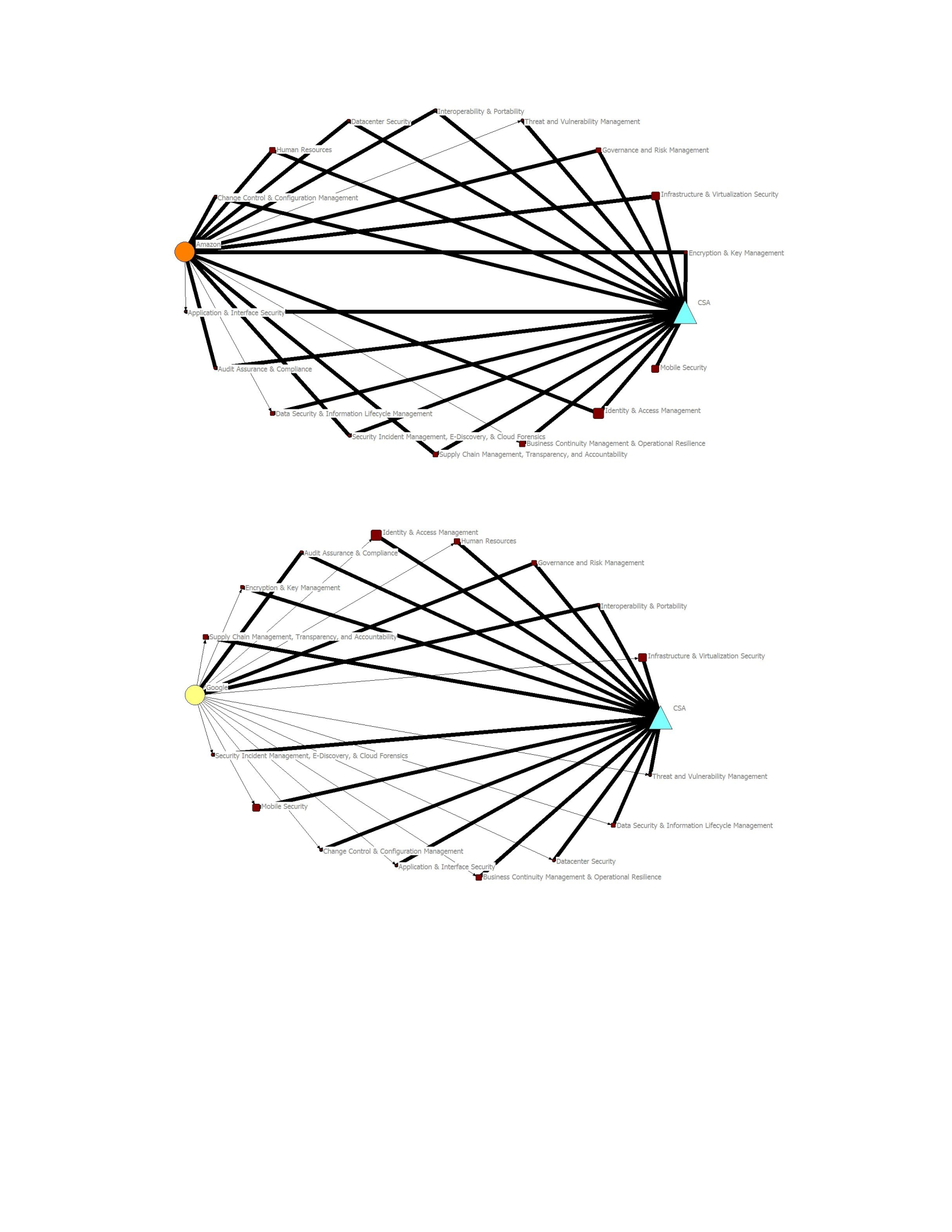
Figure 4-4 Relationships Between CSP Amazon and CSA CCM
91
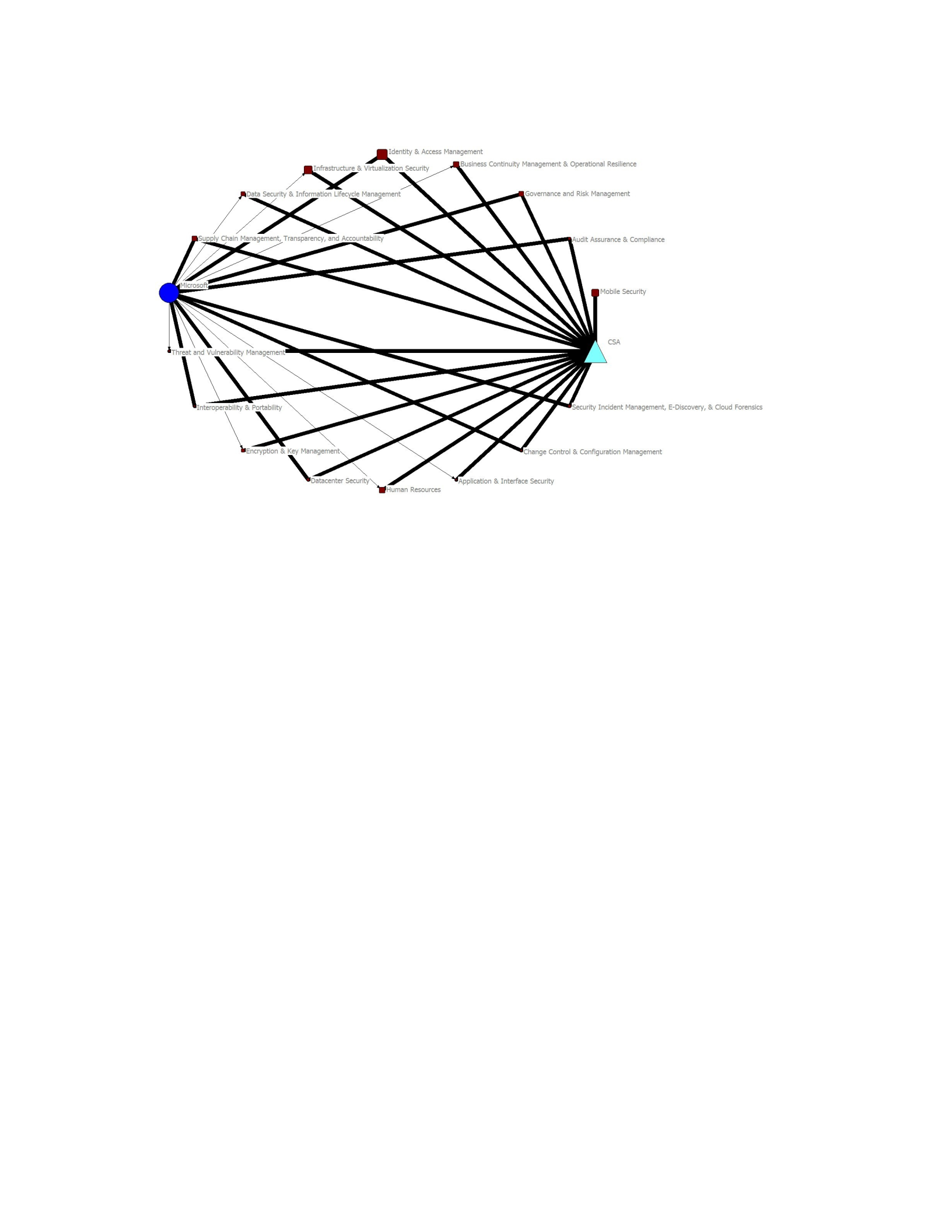
Figure 4-5 Relationships Between CSP Google and CSA CCM
Figure 4-6 Relationships Between CSP Microsoft and CSA CCM
For each control within every control domain, the CAIQ security assessment reports
(CSA CAIQ 2017) consists of a set of control questions (i.e. requirements) which are
assessed to ascertain the CSPs (Amazon, Google, Microsoft) level of CCM compliance.
The node size for each CCM control domain is based on the number of controls and
questions for the domain in proportion to the combined total number of controls and
questions for all control domains. The CSP (Amazon, Google, Microsoft) node sizes are
based on the percentage of total control questions the CSPs comply with (STAR AWS
2017, STAR Google 2017, STAR Microsoft 2017). The thickness (strength) of the
relationships (tie) between a specific CCM control domain and the CSPs (Amazon,
Google, Microsoft) denote the number of control related questions the CSP complies with
for the domain in proportion to the total number of control questions for the domain. The
thickness (strength) of the relationship (tie) between a specific CCM control domain and
CSA denotes the number of control related questions defined by CSA for the specific
92

domain in proportion to the combined total number of control questions defined by CSA
across all domains.
Based on nodes, ties and relationships modeled in Figures 4-4, 4-5, 4-6, Centrality
factors were assessed and the following observations were made (Diestel 2005). Refer to
Appendix I for Degree Centrality details regarding CSA and CSP organizations, and
CCM control domains in terms of CAIQ reports for the CSPs.
•For Figures 4-4, 4-5, 4-6: 3 of the 16 CCM control domains provide a combined
35% of the control requirements questions in the CAIQ (each represented by >=
10% of the 296 total control requirements questions vs the others which ranged
individually between 3% to 8%): Identity & Access Management, Infrastructure
& Virtualization Security, Mobile Security.
•For Figure 4-4 (overall compliance = 87%), Amazon complied with 100% of 8 of
16 control domains (42% of 296 control requirements questions); 7 of 16 control
domains were between 90% and 99% compliance (45% of 296 control
requirements questions: Application & Interface Security; Business Continuity
Management & Operational Resilience; Data Security & Information Lifecycle
Management; Human Resources; Identity & Access Management; Supply Chain
Management, Transparency & Accountability; Threat & Vulnerability
Management); 1 of 16 control domains was at 0% compliance (0% of 296 control
requirements questions: Mobile Security).
•For Figure 4-5 (overall compliance = 87%), Google complied with 100% of 3 of
16 control domains (14% of 296 control requirements questions); 5 of 16 control
domains were between 90% and 99% compliance (27% of 296 control
requirements questions: Change Control & Configuration Management;
93

Datacenter Security; Encryption & Key Management; Human Resources; Mobile
Security); 7 of 16 control domains were between 80% and 89% compliance (44%
of 296 control requirements questions: Application & Interface Security; Business
Continuity Management & Operational Resilience; Data Security & Information
Lifecycle Management; Identity & Access Management; Infrastructure &
Virtualization Security; Security Incident Management, E-Discovery & Cloud
Forensics; Supply Chain Management, Transparency and Accountability); 1 of 16
control domains was at 5% compliance (2% of 296 control requirements
questions: Threat & Vulnerability Management).
•For Figure 4-6 (overall compliance = 85%), Microsoft complied with 100% of 7
of 16 control domains (33% of 296 control requirements questions); 6 of 16
control domains were between 90% and 99% compliance (45% of 296 control
requirements questions: Business Continuity Management & Operational
Resilience; Encryption & Key Management; Human Resources; Identity &
Access Management; Infrastructure & Virtualization Security; Threat &
Vulnerability Management); 2 of 16 control domains were between 80% and 89%
compliance (7% of 296 control requirements questions: Application & Interface
Security; Data Security & Information Lifecycle Management); 1 of 16 control
domains was at 0% compliance (0% of 296 control requirements questions:
Mobile Security).
4.1.6 Review of Graph Theory Approach and Contribution
Graph Theory was used for the research in this Praxis to model cloud SLA work
driven by industry standards organizations (EC, ENISA, ISO/IEC) (EC 2014, Hogben,
94

Giles and Dekker 2012, ISO/IEC 2016) and how it related to the cloud SLAs provided by
the top three CSPs (Amazon, Google, Microsoft) (SLA AWS 2017, SLA Google 2017,
SLA Microsoft 2017), along with cloud security controls from CSA (CSA CCM 2017).
With the modeled graphs, gaps, overlaps and relationships between the organizations
were illustrated.
NetDraw (Borgatti 2002), a network analysis software package, was used for
visualizing the industry standards and CSP cloud SLA and security capabilities. The
following questions drove the Graph Theory modeling and analysis.
•What cloud SLA standards are related to what industry standards organizations
and CSPs?
•What SLAs exist for each CSP?
•What SLAs have interrelationships across CSPs and what are the SLA gaps and
overlaps between the CSPs?
•What are the relationships between the CSP SLAs (Amazon, Google, Microsoft),
industry standards organizations (ISO/IEC, EC, ENISA) and industry cloud SLA
standards (i.e. content areas)?
•Knowing the CCM control domains have some overlap with the SLA standards,
what is the relationship between CSA CCM and cloud SLA standards … where are
the gaps and how strong are the overlaps?
•What relationships exist between the CSA CCM and CSP’s CAIQ (Amazon,
Google, Microsoft)?
•How strong are CSP’s CCM capabilities across each control domain?
95

The primary goal was to analyze and confirm, via Graph Theory, the cloud SLA and
CSP capability structure that would be input to the Analytic Hierarchy Process for
calculating CSP trustworthiness. CSP trustworthiness was ultimately input to Linear
Regression Analysis as one of the predictor variables for predicting cloud SLA
Availability.
Based on the analysis and findings related to the produced graphs, Table 4-1
summarizes how the organizations (standards bodies CSA, EC, ENISA, ISO/IEC; and
CSPs Amazon, Google, Microsoft) contributed to the cloud SLA content areas, and how
they compared with each other’s contribution.
4.2 Analytic Hierarchy Process to Model CSP Trustworthiness
The objective of using Analytic Hierarchy Process (AHP) is to analze and model the
trustworthiness of Cloud Service Providers (CSPs). Assessing CSPs with respect to
multiple factors (e.g. delivery and support capability, security, quality of service,
performance) require a framework to identify and understand the problem, criteria and
their relationships. AHP provides this framework, enabling the problem, CSP capability
and performance, and expectations to be structured into a hierarchic order along with
judgements and numeric values that reflect their importance and impact. The values are
synthesized to determine overall priorities and rankings which ultimately serve to
represent the trustworthiness of the CSP.
There are several dimensions of trustworthiness of a CSP. The principle dimensions
(criteria) that were evaluated by this research related to cloud Service Level Agreement
(SLA) Content Areas based on the Graph Theory Analysis (EC 2014, Hogben, Giles and
Dekker 2012, ISO/IEC 2016). The content areas include: Accessibility; Attestations,
Certifications and Audits; Availability; Change Management; Cloud Service
96

Performance; Cloud Service Support; Data Management; Governance; Information
Security; Protection of PII; Service Reliability; Termination of Service; and a collection
of other important capabilities from CSA CCM (i.e. datacenter security; interoperability
and portability; mobile security; and supply chain management, transparency, and
accountability) (CSA CCM 2017).
As previously noted the objective (goal) of the AHP research was to assess and
calculate CSP trustworthiness. Understanding CSP trustworthiness has multiple benefits
and applications (e.g. when benchmarking and selecting a CSP, assessing SLA
performance and compliance, managing risk including quantitative and qualitative risk
analysis, drive CSP continuous improvement). The focus of this research was to analyze
and predict CSP SLA performance (i.e. Availability), leveraging CSP trustworthiness and
other variables. The aforementioned criteria being assessed and the CSP trustworthiness
calculation is based on is cloud SLA Content Areas. For the research, three CSPs (i.e.
Amazon, Google, Microsoft) were selected as the CSP alternatives whose trustworthiness
was evaluated and compared.
To analyze CSP trustworthiness using Analytic Hierarchy Process (AHP), the
following steps were implemented (Saaty 1980, Saaty 1987, Saaty 1990, Saaty, 2012).
1. Build a structured model that breaks down the CSP trustworthiness problem into a
hierarchy of goals, criteria and alternatives (Figure 3-3). The levels of the
structured hierarchy model are organized as follows:
•The first level defines the goal, which is to calculate CSP trustworthiness.
•Level two of the hierarchy consists of the criteria (previously introduced SLA
Content Areas) that contribute to trustworthiness and that were used to assess
97

and compare each CSP’s capabilities. The criteria are discussed further in
section 4.2.1.
•Level three identifies factors that are related to each criterion in level 2. The
factors are mapped to each level two criterion (SLA Content Area) and are
based low level assessment and performance of the CSPs (e.g. CCM
compliance based on CAIQ assessments, cloud service availability and
reliability). The factors are discussed further in 4.2.1.
•The final level (level three), consists of the three CSPs (Amazon, Google,
Microsoft), whose capability and performance are assessed and compared
based on relationships with level three and two elements.
For the AHP analysis, each level of the hierarchy is evaluated with respect to the
next higher level (e.g. CSPs are compared with respect to the factors for each
criterion, and each criterion is compared to calculate a weight that is applied to
the CSP comparison priorities).
2. Step two derives priorities (i.e. weights) for each criterion (SLA Content Areas).
The weights are a result of pairwise comparison of each criterion in terms of their
influence (impact and importance) to the overall goal of CSP trustworthiness. The
comparisons, priorities and weights are discussed further in section 4.2.2.
3. Step three calculates local priorities with respect to each CSP and SLA Content
Area (step two criteria). The priorities represent the CSPs capability, performance
and impact for each SLA Content Area (step two criteria). The calculation (similar
to step two) is a result of pairwise comparisons of each CSP with respect to each
SLA Content Area (step two criteria). The comparisons and priorities are
discussed further in section 4.2.3.
98

4. The last step (step four), determines the overall priorities of each level 4
alternative (i.e. CSP). After completing step three, all local priorities are grouped
by CSP, weighted based on the step 2 weights for each criterion (SLA Content
Area) and aggregated. The final sum for each CSP represents the overall priority
… Trustworthiness level for the CSP. The higher the value, the higher the trust
level. The final overall CSP priorities from this synthesis is discussed further in
section 4.2.4.
There are many different examples of numerical scales and conditions they satisfy
(e.g. ordinal, interval, ratio, absolute, ratio). Ratio scales “preserve proportionality before
and after normalization” (Saaty 2012). To calculate the SLA Content Area capability and
CSP capability strength, proportions (ratios) were used based on absolute measurements
according to published CSP assessments (CSA STAR 2017, CSA CAIQ 2017, STAR
AWS 2017, STAR Google 2017, STAR Microsoft 2017), cloud security capability
framework standards and compliance assessments (CSA CCM 2017, CSA CAIQ 2017),
CSP performance (Gartner 2017). Uniform unit of measurement and uniform unit of
priority was used to calculate ratios, local priorities, perform weighting, and produce
overall priorities that provide the CSP trustworthiness. With the availability of absolute
measurements from credible sources for calculating the multicriteria ratio scale
measurements and pairwise comparisons, it was decided not to utilize the AHP
fundamental scale of real numbers from 1-9 for pairwise comparisons (Saaty 1980, Saaty
1987, Saaty 1990, Saaty, 2012). The fundamental scale is associated with “intensities of
importance or preferences” for use when performing judgements on paired comparisons
(Saaty 1980, Saaty 1987, Saaty 1990, Saaty, 2012). This process produces a “dominance
matrix of judgements” and a “ratio scale of relative values is derived from each matrix”
99

(Saaty 1980, Saaty 1987, Saaty 1990, Saaty, 2012). With absolute measurement
(alternative option to relative measurement), “standards or grades are determined for each
criterion” (Saaty 1980, Saaty 1987, Saaty 1990, Saaty, 2012). This method is “applicable
in situations where there is considerable prior experience” related to the standard or
grading (Saaty 1980, Saaty 1987, Saaty 1990, Saaty, 2012). With the source of the
measurement data coming from organizations such as CSPs (Amazon, Google,
Microsoft), cloud security standards (Cloud Security Alliance) and industry analyst
(Gartner), their considerable prior experience is globally acknowledged across the cloud
industry.
4.2.1 Capability Ratios for SLA Content Areas and CSPs
Capability ratios for SLA Content Areas and CSPs serve as the input based on
absolute measurements for calculating a ratio based scale for building the comparison
matrices, priority vectors, weighting (based on SLA Content Areas as evaluation criteria)
and overall ranking of the AHP alternatives (i.e. CSPs).
Level two of the AHP hierarchy consists of criteria (previously introduced as SLA
Content Areas) that contribute to trustworthiness and are used to help assess each CSP.
For each SLA Content Area (AHP criteria), capability ratios (Appendix P Table P-1) are
calculated based on the strength and importance value derived during the Graph Theory
Analysis of each SLA Content Area. The capability ratio calculations factor the number
of CCM Control Domains, Controls and CAIQs mapped to each SLA Content Area (CSA
CCM 2017, CSA CAIQ 2017, CSA STAR 2017, STAR AWS 2017, STAR Google 2017,
STAR Microsoft 2017). With pairwise analysis of the SLA Content Area capability ratios,
each criterion’s relative importance and impact is ultimately prioritized. The SLA Content
Area capability pairwise analysis and prioritization (i.e. SLA Content Area comparison
100

matrices and priority vectors) are recorded in Tables P-3 and P-4. The resultant SLA
Content Area capability priorities are then used as weight factors to represent the
importance and impact of each SLA Content Area for comparing CSPs
(Table 3-2).
Level three of the AHP hierarchy consists of the factors (e.g. CCM Compliance for a
CSP based on CAIQ assessments, CSP cloud service historical availability) related to
each level two criterion (Appendix D for CAIQ, Appendix M Table M-1 and M-2 for
availability). Similar to each criterion (i.e. SLA Content Area), a CSP capability ratio was
calculated based on the CSPs performance for all factors organized by SLA Content Area
(Table P-2). The CSP capability ratio calculations factor the level of CCM compliance for
each CSP based on CAIQ assessments (STAR AWS 2017, STAR Google 2017,
STAR Microsoft 2017) and historical cloud service performance (Gartner 2017) for the
CSP. With pairwise analysis of the CSP capability ratios organized by SLA Content
Area, each CSP’s relative performance and capability was ultimately prioritized for each
corresponding SLA Content Area. The CSP capability pairwise analysis and prioritization
(i.e. CSP comparison matrices and priority vectors) are recorded in
Appendix G and H. The resultant CSP capability priorities are then weighted based on
SLA Content Area weighting factors (Table 3-2), and aggregated to represent a CSP
priority (ranking) … trustworthiness level (Tables 4-2, 4-3, 4-4).
Table P-1 represents SLA Content Area capability ratios per CCM (Control Domains,
Controls) and CAIQ. Table P-3 (Comparison Matrix for SLA Content Area capability
criteria) is a matrix that presents the pairwise comparisons of the SLA Content Area
capability ratios from Table P-1 (e.g. Accessibility = 0.0769). The SLA Content Area
Capability ratios are calculated based on overall ratio of CCM Control Domains, Controls
101

and CAIQ that are mapped to the SLA Content Capability vs the total. The ratio
represents the strength, impact and overall importance of the SLA Content Area to a
CSP’s capability, performance and overall trustworthiness.
Table P-2 contains the CSP capability ratios per SLA Content Area. Appendix G
(CSP Comparison Matrices for SLA Content Areas) presents matrices (one for each SLA
Content Area) with pairwise comparisons utilizing CSP capability ratio scores for each
SLA Content Area from Table P-2 (e.g. Accessibility for Amazon = 0.0692). When
performing the pairwise comparisons in each SLA Content Area comparison matrix
(Appendix G), the relationship of CSP capability ratio scores from Table P-2 between two
CSPs is represented as: Vi,ca / Vj,ca (for CSPs Ci and Cj), where Vi,ca represents the value of
content area (ca) capability ratio score for CSP (Ci). The following example demonstrates
the CSP pairwise comparison. When assessing and comparing the Accessibility capability
and performance of Amazon and Google, the relative rank ratio (Ri/j,ca) of 1.0278 (as
calculated below) indicates that Amazon’s Accessibility capability is greater than
Googles. From Table P-2: Amazon Accessibility (Va,Acc) = 0.0692, Google Accessibility
(Vg,Acc) = 0.0674; and from Appendix G (Comparison Matrix for Content
Area: Accessibility), (Va,Acc / Vg,Acc) = 1.0278.
4.2.2 Matrices and Priority Vectors for SLA Content Area Capability Criteria
When assessing SLA Content Area capability criteria, we need to identify their
relative priorities since not all priorities are the same. To calculate the priorities (weights),
a pairwise comparison is performed among all SLA Content Areas using their capability
ratios presented in section 4.2.1. To complete the comparison and priority calculation, a
comparison matrix and priority vector of the SLA Content Area priorities was constructed
per Table P-3 and P-4. The value in each cell of the Table P-3 comparison matrix
102

represents a pairwise comparison (i.e. judgement ratio) calculated based on the SLA
Content capability ratios from Table P-1. Once the comparison matrix was complete, the
judgments for each cell needed to be synthesized. This resulted in performing the
following calculations to produce the overall relative priorities (weights) for each SLA
Content Areas (AHP criteria). These priorities will become critical when they are applied
as weights to the CSP priorities for each SLA Content Area prior to calculating the overall
CSP trustworthiness.
In Table P-3 (Comparison Matrix for SLA Content Area capability criteria), the
matrix represents pairwise comparisons utilizing SLA Content Area capability ratio
scores calculated and presented in Table P-1 (e.g. Accessibility = 0.0769). As reviewed in
section 3.3.2, each cell of the matrix (ajk) represents the importance of the jth item
(relative to the kth criterion). Note, the items that appear in the left-hand column of the
comparison matrix are compared with the items in the top row, producing the ratio value
assigned to the cell. For example, with (aj row) = Accessibility compared to (ak column) =
Availability, we have a ratio = 0.0769 / 0.1154 (Table P-1) = 0.667 (Table P-3). If ajk > 1,
then the jth item is more important than the kth item. If the ajk < 1 (which is the case in
this example), then the jth item(Accessibility) is less important than the kth item
(Availability). If ajk = 1, then the two items have the same importance. Note, the value of
the cell (akj) in the same comparison matrix (Table P-3) is the reciprocal value of (ajk).
Also note that when an SLA Content Area (i.e. AHP criterion) is compared with itself, the
value of the cell (ajj) = 1. This means the ratio of importance when comparing the
criterion against itself is always equal.
In Table P-4 (Priority Vector for SLA Content Area capability criteria), the priority
vector related to the Table P-3 comparison matrix, represents the calculated priorities for
103

each SLA Content Area. These same priorities, are the weights presented in Table 3-2 for
each SLA Content Area. These weights are then used to calculate the overall CSP priority
vectors that ultimately contribute the CSP trustworthiness calculation. In Table P-4, the
comparison matrix from Table P-3 is normalized. The average of each row is then
calculated to produce the priority (weight) of each SLA Content Area (e.g. Accessibility
has a priority of 0.06545). The priority (weight) essentially reflects the
importance/contribution/influence of a SLA Content Area with respect to the others.
According to the SLA Content Area capability criteria priority vector in Table P-4,
Information Security is the most important with a priority = 0.31978 (32%), while
Change Management is the least important with a priority = 0.0222 (2%).
4.2.3 CSP Matrices and Priority Vectors per SLA Content Area
For each CSP (AHP alternative), the strength of their performance and capability with
respect to each SLA Content Area (AHP criterion) is analyzed. The strength was
represented by calculating the CSP relative priorities for each SLA Content Area. Since
these priorities are specifically related to each criterion, they are local priorities vs the
overall CSP priorities derived in section 4.2.4 (Saaty 1980, Saaty 1987, Saaty 1990,
Saaty, 2012). To calculate the local CSP priorities, pairwise comparisons are performed
using the CSP capability ratios of each SLA Content Area presented in section 4.2.1. For
each SLA Content Area, a comparison matrix and priority vector was constructed to
present the corresponding CSP pairwise comparisons and priorities. In Appendix G and
H, there was one comparison matrix and related priority vector for each SLA Content
Area. The value in each cell of the comparison matrices in Appendix G represents a
pairwise comparison (i.e. judgement ratio) calculated based on the CSP Capability ratios
from Table P-2 for the SLA Content Area of the matrix. When performing the
104

comparison, the calculation portrays which CSP has the stronger performance and
capability related to the SLA Content Area of the matrix. Similar to the process described
in section 4.2.2, once the comparison matrix is complete, the judgements for each cell
need to be synthesized. The result is a priority vector for each SLA Content Area with the
local priority for each CSP for that SLA Content Area. These CSP priorities are then used
to build the CSP priority vectors presented in section 4.2.4, which are then weighted and
aggregated to produce the overall CSP trustworthiness.
In Appendix G (Comparison Matrices for SLA Content Areas), the matrix for
Content Area Accessibility represents pairwise comparisons utilizing CSP capability ratio scores
calculated and presented in Table P-2 (e.g. Accessibility for Amazon = 0.0692, Google = 0.0674).
As reviewed in section 3.3.2, each cell of the matrix (ajk) represents the importance of the jth item
(relative to the kth criterion). Note, the items that appear in the left-hand column of the comparison
matrix are compared with the items in the top row, producing the ratio value assigned to the cell.
For example, with (aj row) = Amazon Accessibility compared to (ak column) = Google Accessibility, we
have a ratio = 0.0692 / 0.0674 (Table P-2) = 1.0278 (Appendix G). If ajk > 1 (which is the case in
this example), then the jth item (Amazon Accessibility) is more important than the kth item
(Google Accessibility). If the ajk < 1, then the jth item is less important than the kth item. If ajk = 1,
then the two items have the same importance. Note, the value of the cell (akj) in the same
comparison matrix (Appendix G) is the reciprocal value of (ajk). Also note that when a CSP for the
SLA Content Area (i.e. AHP alternative) is compared with itself, the value of the cell (ajj) = 1. This
means the ratio of importance when comparing the alternative against itself is always equal.
In Appendix H (CSP Priority Vector for SLA Content Areas), the priority vectors
related to the Appendix G comparison matrices, represent the calculated priorities for
each CSP with respect to each SLA Content Area (e.g. CSP Priority Vector for
105

Accessibility = 0.3404, 0.3312, 0.3284). The local CSP priorities in these CSP Priority
Vectors for each SLA Content Area were then used to construct the overall CSP Priority
Vectors in Table 4-2. The CSP Priority Vectors were then weighted (Table 4-3) and
aggregated to ultimately produce the CSP trustworthiness calculations (Table 4-4). In
Appendix H, the comparison matrices from Appendix G were normalized (each column
sum = 1). The average of each row was then calculated to produce the local priority of
each CSP for that SLA Content Area (e.g. Amazon Accessibility has a priority of
0.3404). The priority essentially reflects the performance and capability of a CSP (e.g.
Amazon) with respect to the other CSPs for a specific SLA Content Area. According to
the CSP Priority Vectors for SLA Content Area Accessibility in Appendix H, Amazon has
the highest performance and capability with a priority = 0.3404 (34%), while
Microsoft having the lowest performance and capability with a priority = 0.3284 (33%). A
similar analysis of the other CSP Priority Vectors for the other SLA Content Areas can be
performed.
4.2.4 CSP Priority Vectors and Comparison Trustworthiness Levels
In the final AHP process step, the overall priority for each CSP (i.e. each alternative)
was calculated. In the previous step (section 4.2.3), the priorities were local and reflected
the CSP priority with respect to each individual SLA Content Area (i.e. criterion). With
the overall priority for each CSP, we take into account not only the CSP priorities for each
criterion but also the weighting factor of each criterion (i.e. SLA Content Area).
This ties all levels of the hierarchy together and represents “model synthesis” (Saaty
1980, Saaty 1987, Saaty 1990, Saaty, 2012).
106
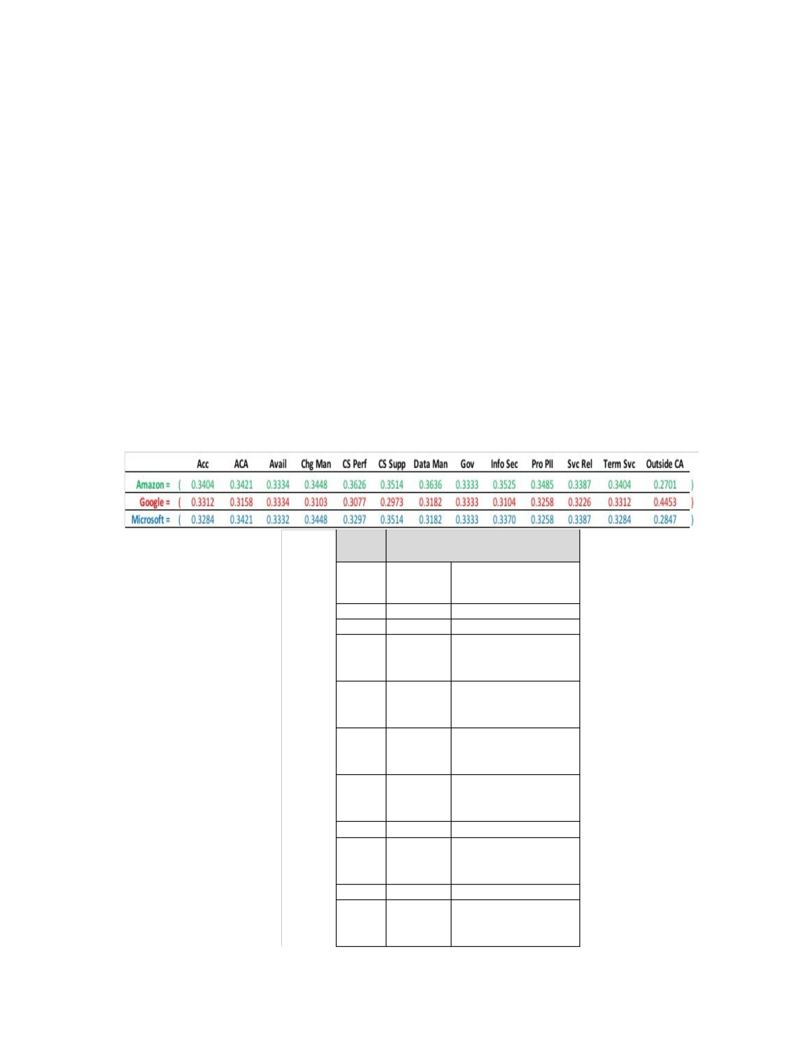
In this step, calculating CSP trustworthiness performs AHP based estimation by
building CSP priority vectors (Table 4-2) based on the CSP Priority Vectors for SLA
Content Areas (Appendix H). The weight factors for each SLA Content Area Criteria
(Table 4-2) are then applied to the CSP priority vectors (i.e. each SLA Content Area
weight factor was multiplied by each priority in the CSP priority vector) to build the
weighted CSP priority vectors (Table 4-3). The calculation of the weight factors
(presented in Table 4-2) were based on the priority vectors for SLA Content Area
Capability Criteria (Table P-4). Finally, the trustworthiness level for each CSP was
calculated by aggregating the weighted CSP Priority Vectors (Table 4-4).
Table 4-2 CSP AHP Based Estimation – CSP Priority Vectors and weighting factors
Weight SLA Content Area
Criteria
X0.0655 Acc AccessibilityAttestations,
Certifications
and
0.0236 ACA Audits
0.0982 Avail Availability
0.0222 Chg
Man
Change Management
0.0653 CS
Perf
Cloud Service
Performance
0.0264 CS
Supp
Cloud Service
Support
0.0348 Data
Man
Data Management
0.0473 Gov Governance
0.3198 Info
Sec
Information
Security
0.1029 Pro PII Protection of PII
0.0487 Svc
Rel
Service Reliability
107
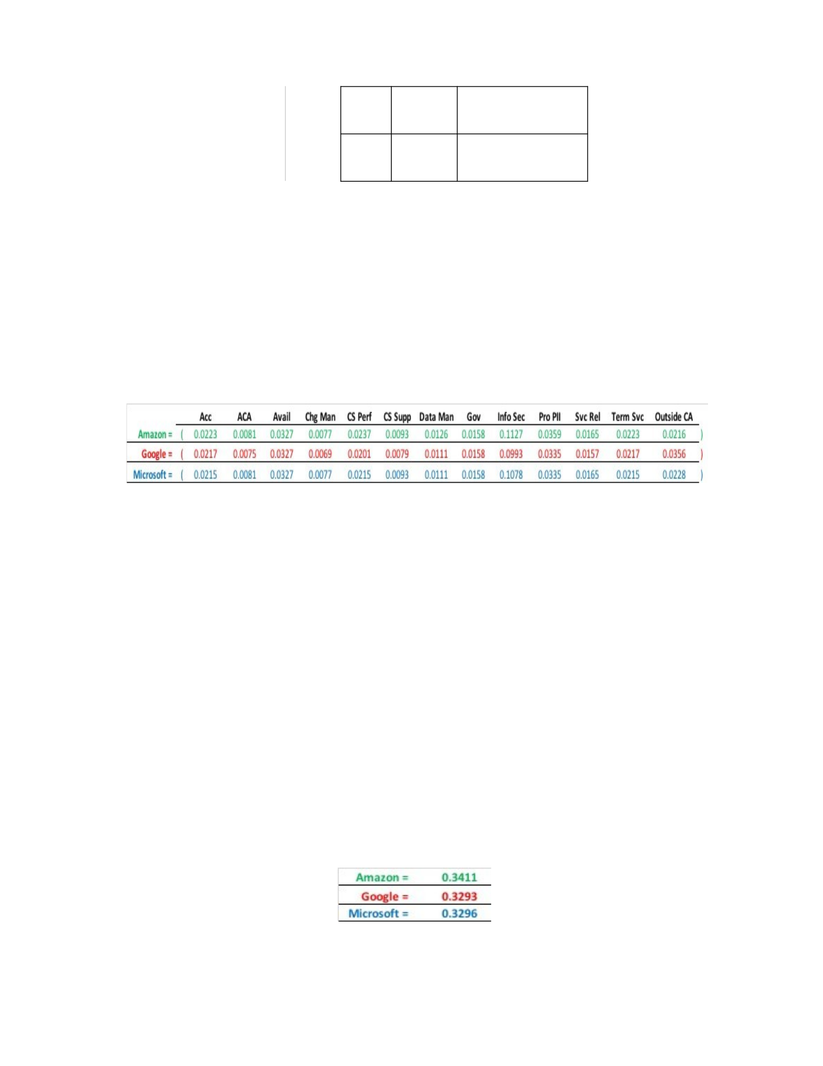
0.0655 Term
Svc
Termination of
Service
0.0799 Outside
CA
Capability outside SLA
CAs
For each CSP Priority Vector per Table 4-2, each SLA Content Area priority entry was
multiplied by their corresponding SLA content area criteria weight (e.g. 0.655 for
Accessibility multiplied by Acc = 0.3404 for Amazon => 0.0223). The result was the
weighted AHP based estimation for each CSP as represented in Table 4-3, i.e. weighted
priority vectors for each CSP.
Table 4-3 CSP AHP Based Estimation – weighted CSP Priority Vectors
For each CSP, the weighted priority vector entries for all SLA Content Areas from
Table 4-3 are aggregated to represent the final overall priorities for the CSPs. The final
overall priorities from this synthesis represent the comparative trustworthiness level for
each CSP (Table 4-4). The composite priority for each CSP with respect to all factors for
each criterion from the hierarchy structure, shows the relative trustworthiness ranking of
the CSPs on an overall basis. This is an example of a complete hierarchy since all factors
(e.g. level three in the hierarchy) relate to the criteria at the next level (e.g. level two in
the hierarchy). The higher the CSP ranking, the higher the level of CSP trustworthiness
(Saaty 1980, Saaty 1987, Saaty 1990, Saaty, 2012).
Table 4-4 CSP Comparison Trustworthiness Levels
108

With Table 4-4, we now have the CSP trustworthiness levels that can be leveraged for
comparison of the CSPs. We can see that Amazon represents the highest level of
trustworthiness (i.e. 0.3411), while Google represents the lowest. In other words, given
the importance (weight) of each SLA Content Area (i.e. evaluation criteria), Amazon is
the most trusted of the three CSPs.
4.2.5 Absolute CSP Trust Level for Linear Regression
The AHP based approach and estimated CSP trustworthiness levels calculated in
section 4.2 are effective for comparing the capabilities of two or more specific CSP’s
against each other. The ultimate objective for the research study of this Praxis is to
provide the Linear Regression Analysis presented in section 4.3 with an absolute (vs
relative) trust level that reflects each CSP’s independent capabilities. This requires the
application of the same methodology presented in section 4.2 but with pairwise
comparisons of each CSP’s capabilities against a virtual CSP that is scored with
maximum capabilities from Table P-2 (CSP capability ratios per SLA Content Area). A
similar comparison matrix to Appendix G (CSP Comparison Matrices for SLA Content
Areas) and similar resultant priority vectors to Appendix H (CSP Priority Vectors for SLA
Content Areas) for each CSP will be calculated (e.g. Table 4-5 presents an example for
Amazon and the Accessibility SLA Content Area). The same process is then implemented
as outlined for Tables 4-2, 4-3, 4-4. For the Amazon example, the resultant
Priority Vector, Weighted Priority Vector and Absolute Trust Level is presented in Table
4-5. As depicted in Table 4-5, after aggregating Amazon’s Weighted Priority Vector, the
absolute CSP trust level was calculated. The absolute trust level is a ratio (between 0 and
1) of the CSP’s capability vs the maximum potential and is leveraged as a predictor
variable for the Linear Regression Analysis in section 4.3.
109
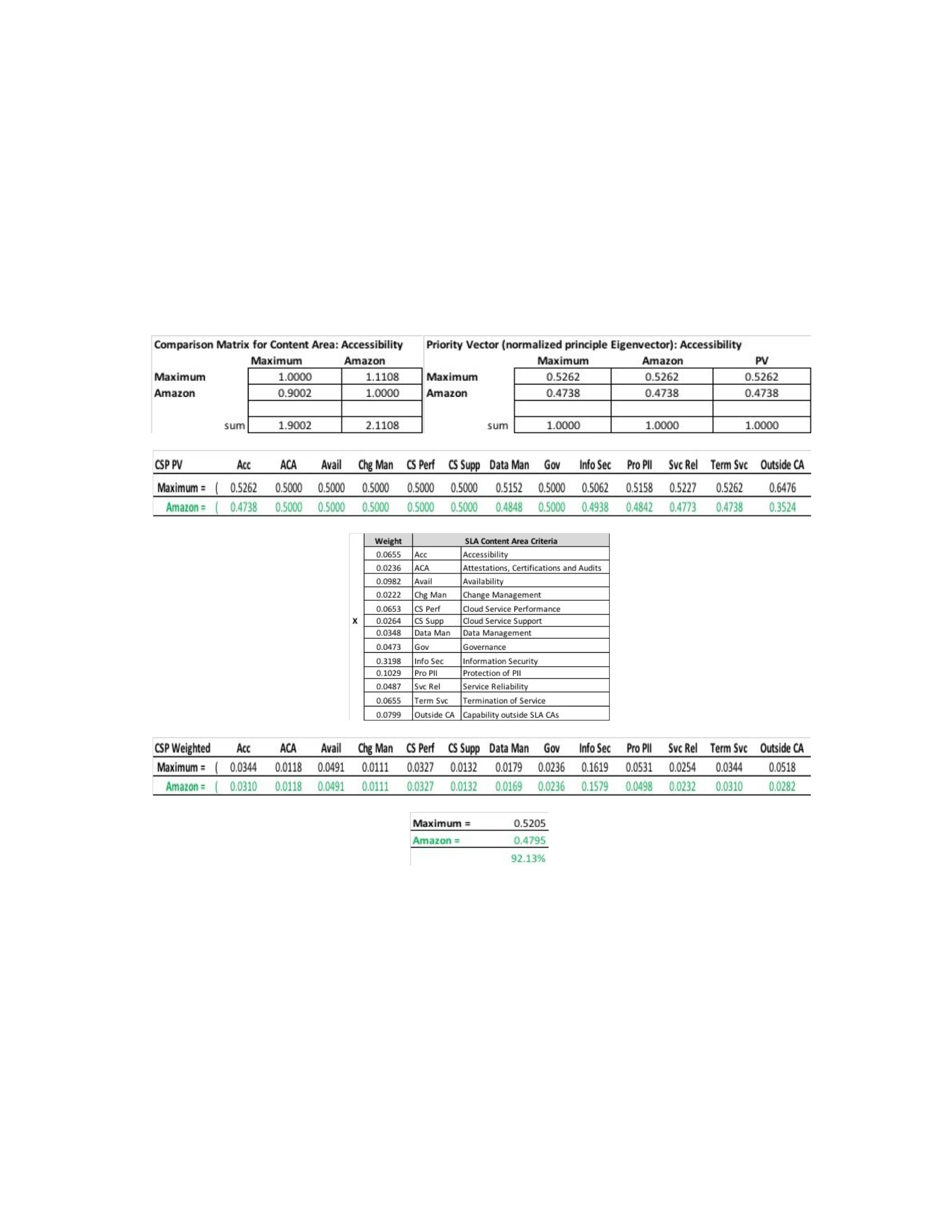
As already introduced, Table 4-5 depicts the AHP based estimation for calculating
Amazon’s absolute trust level of 92.13%. Absolute trust levels for Google (88.6%) and
Microsoft (89.13%) were calculated in the same manner. Only matrix and priority vector
for content area Accessibility is demonstrated.
Table 4-5 Example Calculation of Independent CSP Trust Level for Linear Regression
4.3 Linear Regression to Model and Predict Cloud SLA Availability
Two linear regression models (simple variable and multiple variable) were created to
relate predictor variables with the response variable and drive predictions that enable
analysis and testing of the stated hypothesis. This chapter is organized by the regression
analysis of two models, their comparison, hypothesis testing, and applications. As
110

introduced in chapter 3 (Methodology), RStudio, an integrated development environment
for statistical computing and graphics, was utilized for the regression analysis (Chatterjee
and Hadi 2013, Kutner, Nachtsheim and Neter 2008, Harrell 2015).
4.3.1 Simple Regression Model
The simple linear regression model is denoted by the equation Y=B0 + B1X + E where
B0 and B1 represent the regression coefficients and E is the “random disturbance or error”
(Chatterjee and Hadi 2013, Kutner, Nachtsheim and Neter 2008). For the model, the goal
was to estimate parameters B0 and B1 and “find the straight line that provided the best fit”
of the response versus predictor variable using least squares method (Chatterjee and Hadi
2013, Kutner, Nachtsheim and Neter 2008).
4.3.1.1 Simple Regression Model Datasets and Variables
The datasets used for the regression analysis represent 101 observations related to
response variable cloud service Availability along with 5 predictor variables (Downtime,
Trust, Performance, Location, Regions). While the multiple linear regression analysis
leveraged all predictor variables, the simple regression analysis focused on the single
predictor Downtime. Downtime refers to the number of minutes of cloud compute service
downtime. With the histograms presented in Figure 4-7, we can identify patterns in the
availability percentages and minutes of downtime datasets. On each histogram, the blue
vertical lines represent median values and the red lines average values. On both
histograms, it’s clear outliers exist that will require further analysis as we fit a linear
regression model to the observations and test linear regression assumptions (e.g. linearity,
normality, homoscedasticity, and outliers).
111
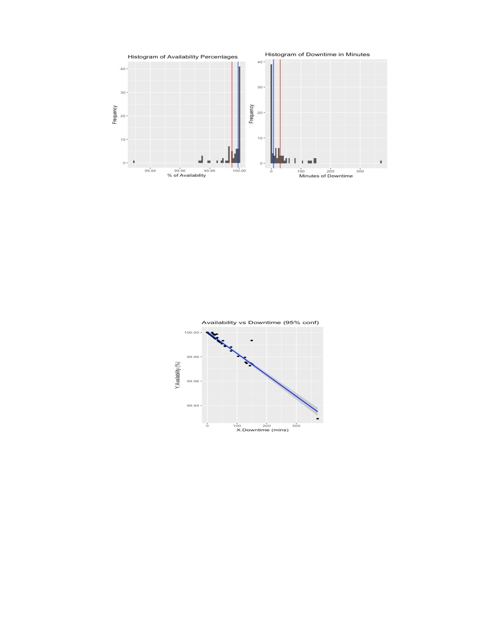
Figure 4-7 Histogram of Availability and Downtime for Simple Regression (Initial)
The scatterplot of both variables (Availability, Downtime) in Figure 4-8 depicts their
relationship. Each data point on the graph represents an observation related to the
relationship for a cloud service provider (CSP) compute service region. We can observe
how the percentage of Availability changes as minutes of cloud compute service
Downtime increases.
Figure 4-8 Scatterplot of Availability and Downtime for Simple Regression (Initial)
4.3.1.2 Simple Regression Model (Initial)
For the initial simple linear regression model Equation 4.1, I solved for the following
equation using the R lm function (Equation 4.2) to fit the linear model based on Least
Squares. The output from Equation 4.3, the R summary in Figure 4-9 is presented and
analyzed below.
112
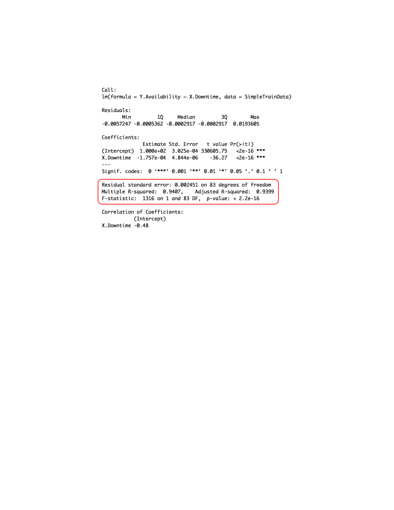
Y.Availability = B0 + B1 * X.Downtime (4.1)
R: SimpleModel = lm(Y.Availability ~ X.Downtime, data=SimpleTrainData) (4.2)
R: summary(SimpleModel,4) (4.3)
Figure 4-9 Simple Regression Summary (Initial)
From the Figure 4-9 model summary output (see red circle) and the Figure 4-8
variable scatterplot we can make the following observations.
•The scatterplot depicts that the relationship between Availability and Downtime
follows a straight line. While just this observations is not a enough of an
indication of linearity, it suggests the relationship is linear. However, note the
fitted line does not align with a pattern across all data points.
•The p-value, an overall test of the statistical significance for the model, is very
close to zero and the model produced a strong R-squared.
•The R-squared (i.e. coefficient of determination) measure indicates that majority
of variance related to Availability is explained by Downtime. The closer the
Rsquared value is to 1, the better the model explains the variance.
113

•The R-squared value for the model is 0.9407 (adjusted 0.9399), which is a high
score. This suggests the linear model’s fit to the data explains 94% of the variance
observed in the data.
•The residual standard error, which is 0.002451, measures the average amount of
Availability that “deviates from the true regression line for any given point” (i.e.
how far observed Y values are from the predicted values) (Tattar, Ramaiah, and
Manjunath 2016, Chatterjee and Hadi 2013). This means that in the model, any
Availability prediction based on Downtime will be off by an average of 0.002451,
which is a small number. The Intercept is the “estimated mean Y value” when X is
zero (i.e. the estimated mean Availability value when Downtime is zero) (Tattar,
Ramaiah, and Manjunath 2016, Chatterjee and Hadi 2013).
•So, given the residual standard error for Availability is 0.002451 and the mean
Availability value is 1.000e+02 (Intercept), we can assume that the average
percentage error for any given point is 0.002451% (0.002451/1.000e+02 =
2.451e-05). This is also a small error rate (Tattar, Ramaiah, and Manjunath 2016,
Chatterjee and Hadi 2013).
After analysis and interpretation of the model’s results related to key linear regression
assumptions, transformation of the predictor variable Downtime was required in addition
to removal of two outlier data points in order to satisfy the assumptions. Assumptions not
met by the model without these changes included linearity, normality, homoscedasticity,
and outliers. The plots in Figure 4-10 review the outlier analysis and removal based on
the two R functions in Equations 4.4 and 4.5:
R: ols_rsdlev_plot(SimpleModel) (4.4)
R: ols_dffits_plot(SimpleModel) (4.5)
114
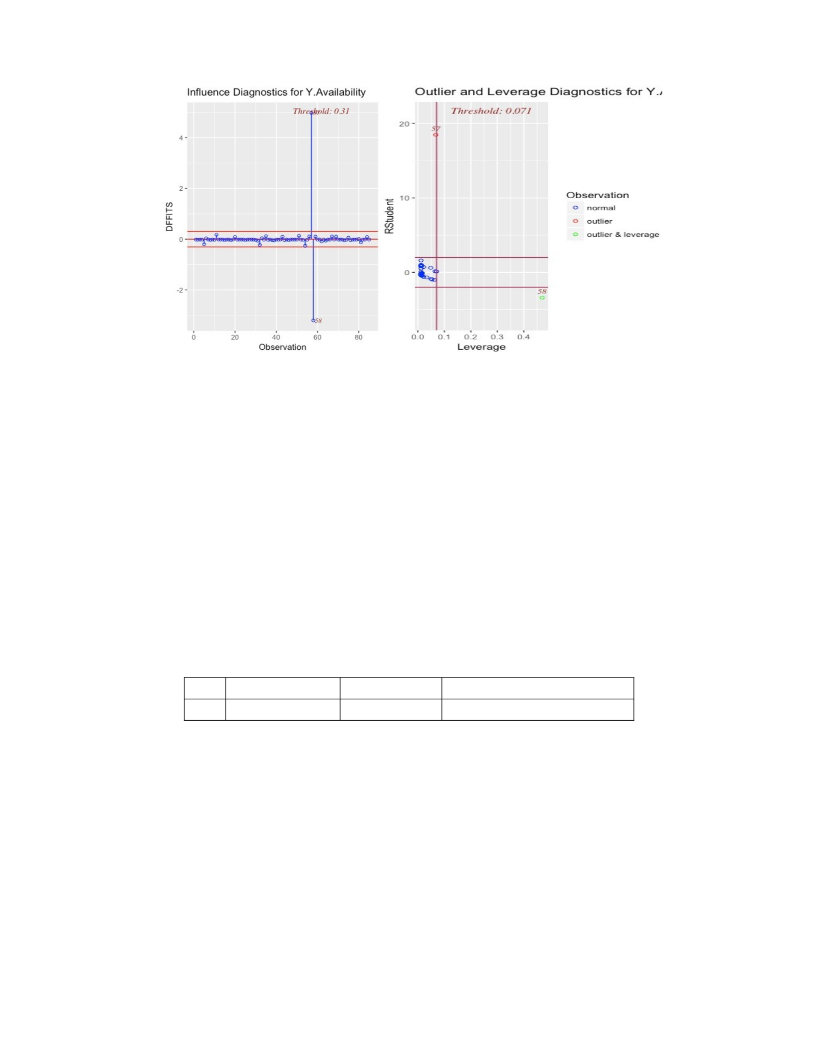
Figure 4-10 Simple Regression Model (Initial) Outliers Plots
Per the Figure 4-10 plots, two outliers were identified in Table 4-6. These data points
lie away from the regression line and subsequently have high residual values. Per the
analysis summary below, the outlier data points represent erroneous data and do not
influence the regression analysis. The following Equation 4.6 R command identifies the
outlier data points from the plots.
R: SimpleTrainData[c(57,58),] (4.6)
Table 4-6 Outliers Removed from Simple Regression Train Dataset
ID Y.Availability X.Downtime
39 99.9934 149.4 Microsoft asia-east outage
101 99.9292 372.0 Microsoft us-west2 outage
Removal of the outlier data point (39) is based on the observation having a Downtime
value inconsistent with the required Downtime value to calculate the corresponding
observed Availability. Removal also addresses linear model assumption issues (i.e.
normal distribution) and has minimal impact to the model (i.e. regression line slope is
roughly the same). With the removal, R Squared remains strong, estimated regression
115

coefficients and standard errors of the regression coefficients have little change, and
Pvalue has little change.
Also, after analysis the outlier and high leverage data point(101) is explained by an
extended maintenance window for a specific CSP and service region versus the other data
points in the dataset which are representative of unplanned outages (excluding planned
maintenance windows) (Gartner 2017, CloudHarmony (2017). This data point is a remote
point with almost no effect on the regression coefficients because it lies almost on the line
passing through the other remaining observations. The corresponding residual for the
observation is not unusually large. It indicates that the observation had little influence on
the fitted model. However the data point has a disproportionate impact on the linear
model assumptions. The following analysis in Table 4-7 illustrates the coefficient and
RSquared impact before and after removing the outliers. The updated Figure 4-11
scatterplot of both variables (Availability, Downtime) depicts their relationship with the
outliers removed. Each data point on the graph represents an observation related to the
relationship for a cloud service provider (CSP) compute service region. We can observe
how the percentage of Availability changes as minutes of cloud compute service
Downtime increases.
Table 4-7 Effect of Removing Outliers from Simple Regression Train Dataset
ID Coefficient R-Squared
39 and 101 in -1.757e-04 0.9407
39 and 101 out -1.793e-04 0.9782
116
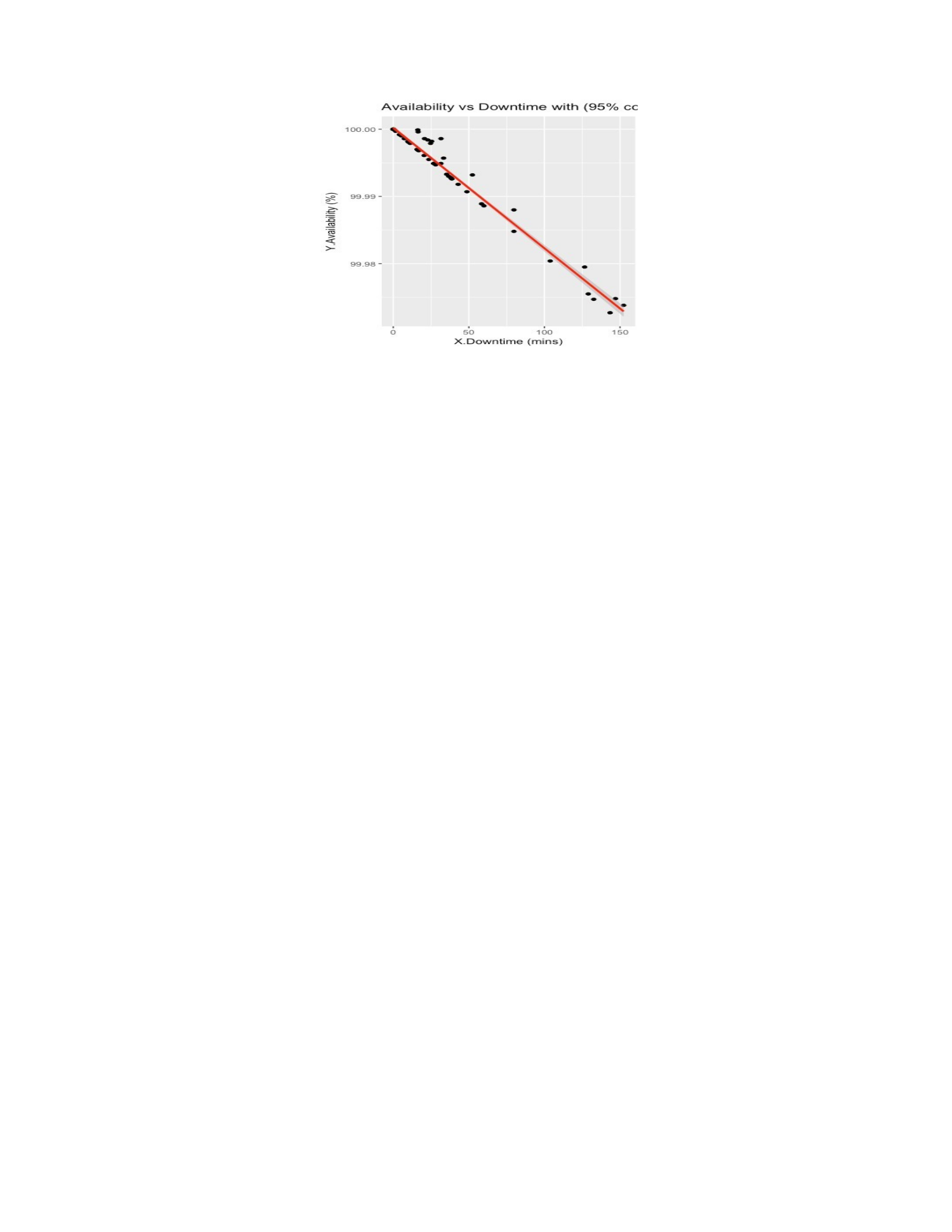
Figure 4-11 Scatterplot of Availability and Downtime for Simple Regression (Modified)
4.3.1.3 Simple Regression Model (Modified)
For the modified simple linear regression model, I solved for Equation 4.7 using the R
lm function in Equation 4.8 to fit the linear model based on Least Squares with the
transformed predictor variable Downtime. The Figure 4-12 output from the R summary
Equation 4.9 is presented and analyzed in the following section.
Y.Availability = B0 + B1 * sqrt(X.Downtime) (4.7)
R: SimpleModelExclude = lm(Y.Availability ~ sqrt(X.Downtime),
data=SimpleDataExclude) (4.8)
4.3.1.3.1 Simple Regression Model Summary
The modified linear regression model output (based on the R summary function) is
analyzed below.
R: summary(SimpleModelExclude,4) (4.9)
117
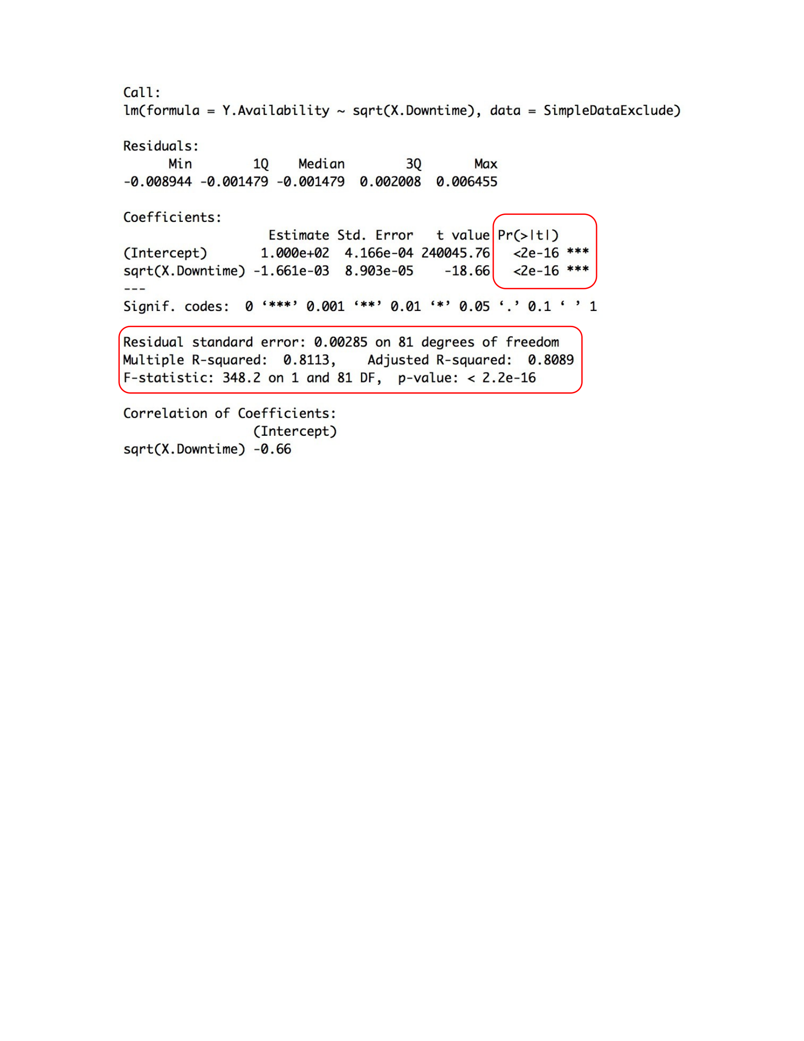
Figure 4-12 Simple Regression Summary (Modified)
In the modified model summary output from Figure 4-12 (see red circle) and modified
variable scatterplot Figure 4-11, we can make the following observations.
•The Figure 4-11 modified scatterplot (minus the removed outliers) continues to
depict the relationship between Availability and Downtime following a straight
line. Again, while just this observations is not a enough of an indication of
linearity, it suggests the relationship is linear. More analysis is provided in a
section below regarding linear regression assumptions for the model.
•The p-value, an overall test of the statistical significance for the modified model,
is still very close to zero and the modified model continues to produce a
reasonably strong R-squared.
118

•The R-squared is 0.8113 (adjusted 0.8089), a high score. This suggests the
modified linear model fit against the data is explaining 81% of the variance
observed in the data.
•Looking at the coefficients, we can observe the dynamics related with response
variable Availability as we plug the coefficient values into the regression equation
to get predicted Availability values. The p-value for the predictor is < 0.05, so we
can say it is significant.
•Another noteworthy observations from the model output is the residual standard
error which measures the average amount of Availability that “deviates from the
true regression line for any given point” (i.e. how far observed Y values are from
the predicted values) (Tattar, Ramaiah, and Manjunath 2016, Chatterjee and Hadi
2013). In the model, any prediction of Availability on the basis of Downtime will
be off by an average of 0.00285, a small number.
•Based on the residual standard error for Availability of 0.00285 and the mean
Availability value of 1.000e+02 (Intercept), we can assume that the average
percentage error for any given point is 0.00285% (0.00285/1.000e+02 = 2.85e05).
Again, a small error rate (Tattar, Ramaiah, and Manjunath 2016, Chatterjee and
Hadi 2013).
4.3.1.3.2 ANOVA of Simple Regression Model
We can analyze the ANOVA results related to the model using the R ANOVA
function in Equation 4.10.
R: anova(SimpleModelExclude) (4.10)
119
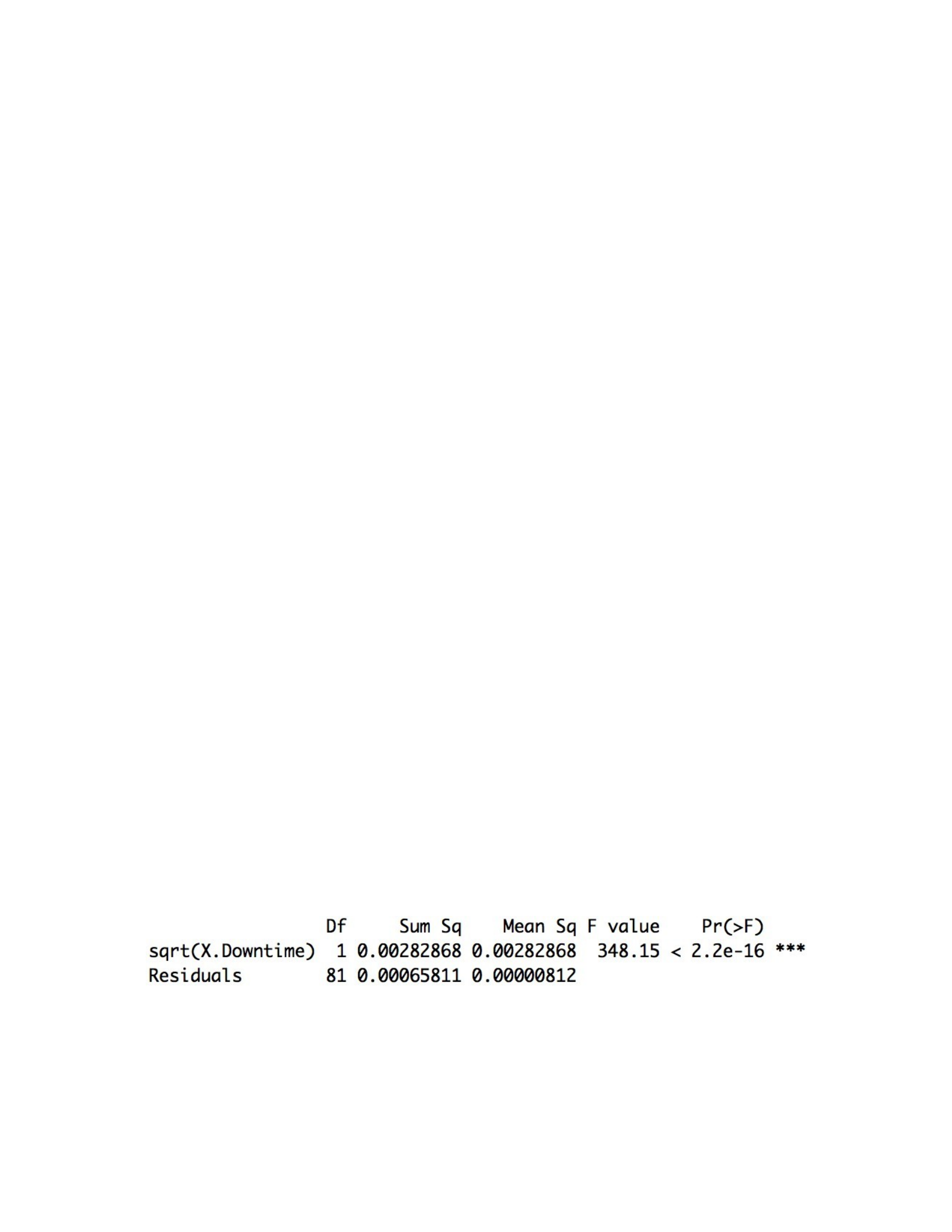
Looking at the following table (Table 4-8), we check the ANOVA F-test results to confirm
a linear relationship exists between Availability and Downtime. The F value column
contains F-test statistic = 348.15, and the Pr(>F) column (= 2.2E-16) contains the P-
value associated with the F-test. The F-test tells us “there is enough statistical evidence
to conclude a linear relationship exists” between Availability and Downtime (Tattar,
Ramaiah, and Manjunath 2016). The Regression Sum of Squares column (= 0.00282868),
quantifies “how far the estimated regression line is from the no relationship line” (i.e. a
horizontal line) (Tattar, Ramaiah, and Manjunath 2016). The Residuals (Error) Sum of
Squares (= 0.00065811), represents “how much the observed data points vary around
estimated regression line” (Tattar, Ramaiah, and Manjunath 2016). The total variation
related to observed Availability is the sum of two parts (i.e. variation due to Downtime =
0. 00282868 and variation due to random error = 0.00065811). From the analysis, we can
conclude Downtime is associated with Availability and there is a linear association
between the two since the “Regression Sum of Squares is the larger component of the
total sum of squares” (Tattar, Ramaiah, and Manjunath 2016). We can also conclude that
most of the variation related to observed Availability data points is attributed to the
predictor variable Downtime vs “random error,” which is what we are looking for (Tattar,
Ramaiah, and Manjunath 2016).
Table 4-8 ANOVA of Simple Regression Model (Modified)
4.3.1.3.3 Simple Regression Model Assumptions
To further assess the linear regression model and the relationship between Availability
and Downtime, compliance with key assumptions (as previously introduced in the chapter
120

3 Methodology) related to Linearity, Normality, Independence, Homoscedasticity, and
Outliers is analyzed and presented in Appendix J (Fox 1991,
Chatterjee and Hadi 2013, Tattar, Ramaiah, and Manjunath 2016).
4.3.2 Multiple Regression Model
The multiple linear regression model is denoted by the equation Y=B0 + B1X1 + B2X2
+ B3X3 + B4X4 + B5X5 + E, where B0, B1, B2, B3, B4, B5 are the regression coefficients,
and E is the random disturbance or error. For the model, the goal is to estimate parameters
B0, B1, B2, B3, B4, B5 and “find the straight line that provided the best fit” of the response
versus predictor variables using least squares method (Chatterjee and Hadi
2013, Kutner, Nachtsheim and Neter 2008).
4.3.2.1 Multiple Regression Model Datasets and Variables
The datasets used for the regression analysis represent 101 observations related to
response variable cloud service Y.Availability along with 5 predictor variables
(X1.Downtime, X2.Trust, X3.Location, X4.Regions, X5.Performance). While the simple
regression analysis focused on a single predictor (X.Downtime) and its related
observation data, the multiple regression analysis focused on all 5 predictors and their
corresponding observation values. Note, the simple regression model is nested in the
multiple regression model. With the following variable matrix scatterplot (Figure 4-13),
we can identify patterns and relationships among the response variable and predictor
variables. For example, we can see how Y.Availability and X5.Performance are related
(e.g. see first column, bottom row). Another interesting example was the relationship
between number of X4.Regions and X5.Performance. As the number of service regions
increase so does performance and downtime (i.e. increases in service regions represent
increases in consumption of compute services and potential for exceeding capacity which
121
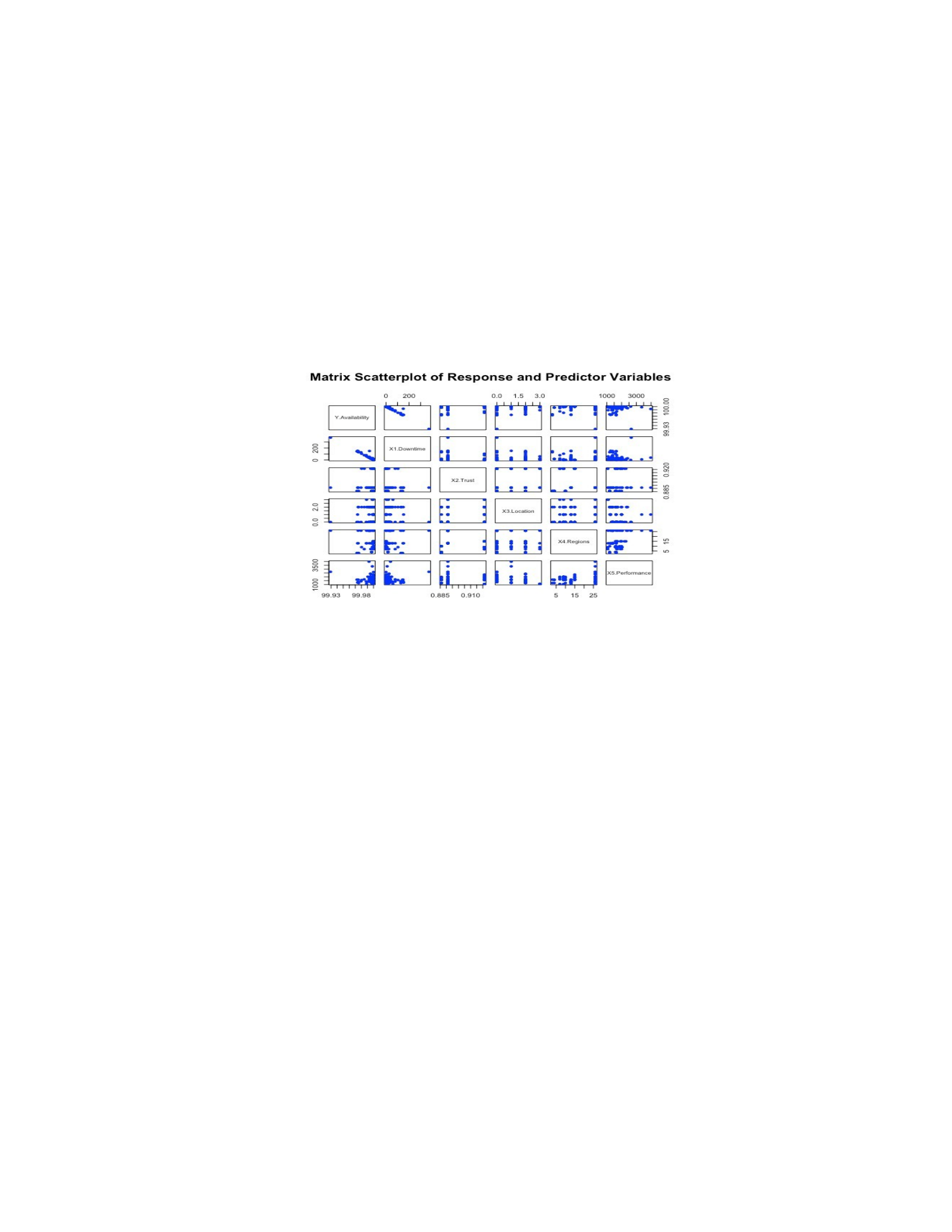
can effect downtime). Also note how X4.Regions seems to have a similar pattern relative
to X2.Trust when plotted against Y.Availability. Similar to the simple regression analysis,
the same outliers exists related to Availability and Downtime so further analysis was
required as the linear regression model was fit to the observations and the linear
regression assumptions were tested (e.g. linearity, normality, independence,
homoscedasticity, and outliers).
Figure 4-13 Matrix Scatterplot of Variables for Multiple Regression (Initial)
4.3.2.2 Multiple Regression Model (Initial)
For the initial multiple linear regression model (Equation 4.11), I solved for the
following equation (Equation 4.12) using the R lm function to fit the linear model based
on Least Squares. The output (Figure 4-14) from the R summary (Equation 4.13) is
presented and analyzed below.
Y.Availability = B0 + B1 * X1.Downtime + B2 * X2.Trust + B3 * X3.Location + B4 *
X4.Regions + B5 * X5.Performance (4.11)
R: MultipleModel = lm(Y.Availability ~ X1.Downtime + X2.Trust + X3.Location
+ X4.Regions + X5.Performance, data=MultipleTrainData) (4.12)
R: summary(MultModel,4) (4.13)
122
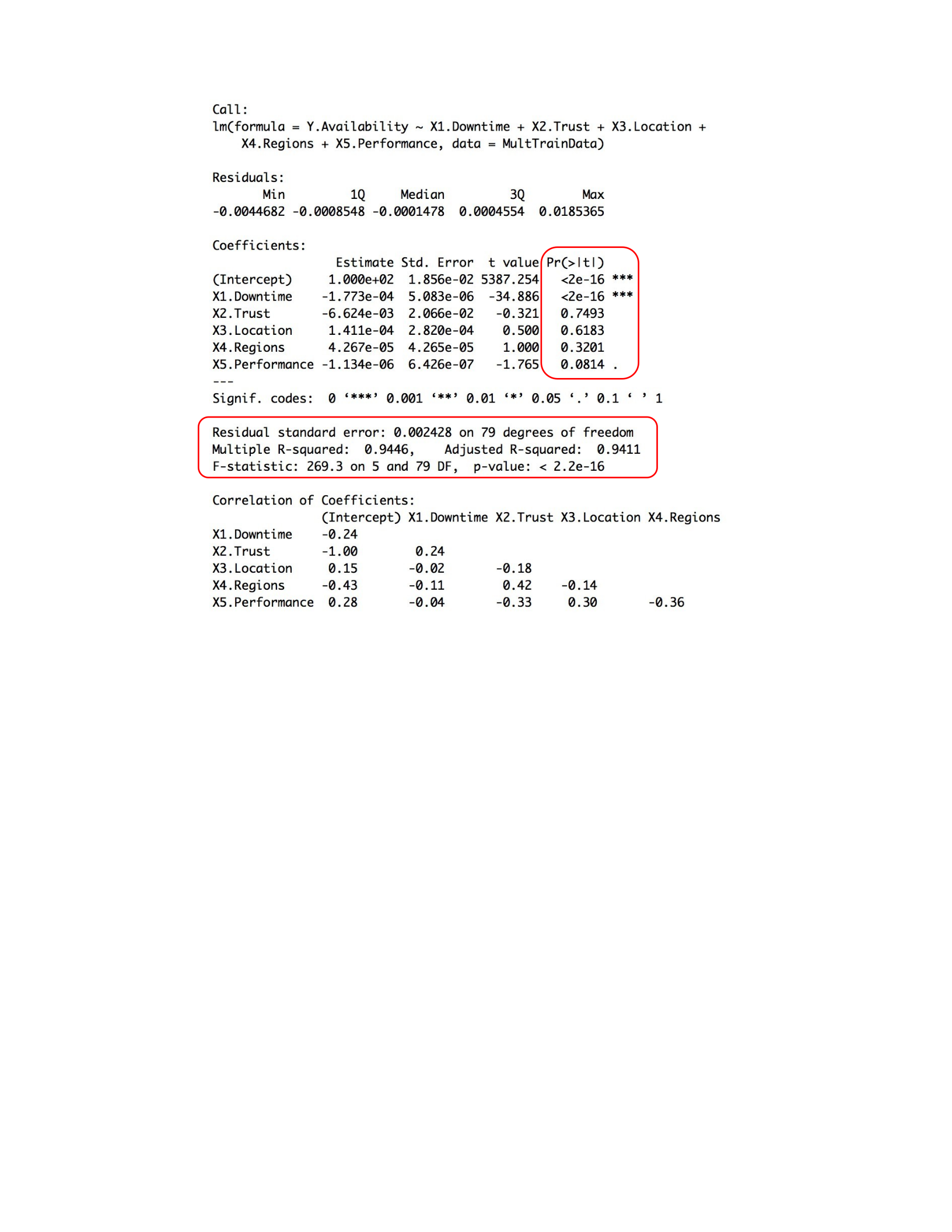
Figure 4-14 Multiple Regression Summary (Initial)
From the Figure 4-14 model summary output (see red circle) and the Figure 4-13
variable scatterplot we can make the following observations.
•The p-value, an overall test of the statistical significance for the model, is very
close to zero and the model produced a strong R-squared.
•The R-squared we get is 0.9446 (adjusted 0.9411), which is a high score. This
suggests the linear model we just fit in the data is explaining 94% of the variance
observed in the data.
•The residual standard error, which measures the average amount of Availability
that will deviate from the true regression line for any given point, is 0.002428.
This means that in the model, any prediction of Availability on the basis of the
123
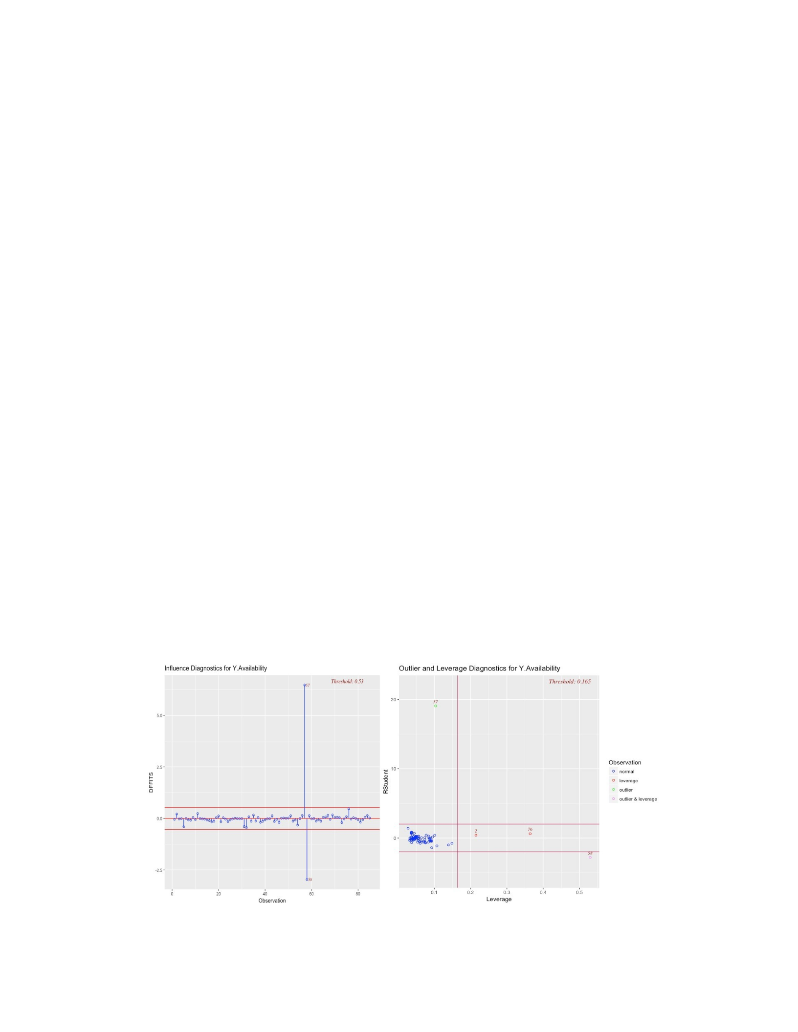
predictor variables will be off by an average of 0.002428, which is a small
number.
•So, given that the residual standard error for Availability is 0.002428 and the
mean Availability value is 1.000e+02 (Intercept), we can assume that the average
percentage error for any given point is 0.002428% (0.002428 /1.000e+02 =
2.428e-05). Again, a small error rate (Tattar, Ramaiah, and Manjunath 2016,
Chatterjee and Hadi 2013).
After analysis and interpretation of the model’s results related to key linear regression
assumptions, transformation of the predictor variables was required in addition to
management of variable interaction and correlation, and removal of two outlier data
points (similar to simple regression analysis) in order to satisfy the assumptions.
Assumptions not met by the model without these changes included normality and outliers.
The following plots Figure 4-15) review the outlier analysis and removal based on the
two R functions (Equation 4.14 and 4.15):
R: ols_rsdlev_plot(MultModel) (4.14)
R: ols_dffits_plot(MultModel) (4.15)
124

Figure 4-15 Multiple Regression Model (Initial) Outliers Plots
Per the Figure 4-15 plots, two outliers were identified (Table 4-9). These data points
lie away from the regression line and subsequently have high residual values. Per the
analysis summary below, the outlier data points represent erroneous data and do not
influence the regression analysis. The following R command (Equation 4.16) identifies
the outlier data points from the plots (Table 4-9).
R: MultTrainData[c(57,58),] (4.16)
Table 4-9 Outliers Removed from Multiple Regression Train Dataset
ID Y.Availability X1.Downtime X2.Trust
39 99.9934 149.4 0.8913
101 99.9292 372.0 0.8913
X3.Location X4.Regions X5.Performance
2 26 1386 Microsoft asia-east outage
0 26 2655 Microsoft us-west2 outage
Similar to the simple regression analysis, removal of the outlier data point (39) was
based on the observation having a X1.Downtime value inconsistent with the required
X1.Downtime value to calculate the corresponding observed Y.Availability. Removal
also addresses linear model assumption issues (i.e. normal distribution) and has minimal
impact to the model (i.e. regression line slope is roughly the same). With the removal, R
Squared remains strong, estimated regression coefficients and standard errors of the
regression coefficients have little change, and P-value has little change.
Also (similar to the simple regression analysis), the outlier and high leverage data
point(101) is explained by an extended maintenance window for a specific CSP and
service region versus the other data points in the dataset which are representative of
unplanned outages (excluding planned maintenance windows) (Gartner 2017,
125
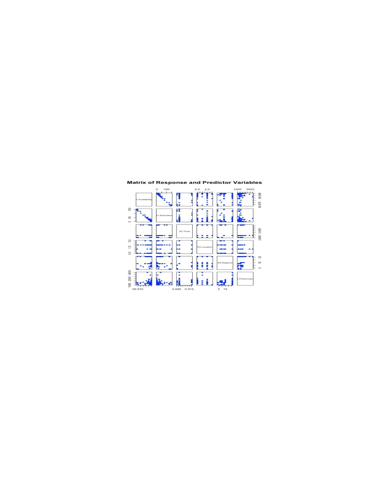
CloudHarmony (2017). This data point was a remote point with almost no effect on the
regression coefficients because it lies almost on the line passing through the other
remaining observations. The corresponding residual for the observation was not unusually
large. This indicates that the observation has little influence on the fitted model. However,
the data point has a disproportionate impact on the linear model assumptions. After
removing the two data points, the following variable matrix scatterplot (Figure 4-16) can
help identify any patterns and relationships among the response variable and predictor
variables.
Figure 4-16 Matrix Scatterplot of Variables for Multiple Regression (Modified)
4.3.2.3 Multiple Regression Model (Modified)
The following methods (based on the noted R functions, Equations 4.17 – 4.25) were
implemented to select the predictor variables and final model: stepwise selection
(forward, backward, both using AIC), all-subset regression using leaps, and lastly best
subset selection.
• Stepwise regression to identify the model with the lowest AIC:
R: MultModelEBase <- lm(MultDataExclude$Y.Availability ~ 1,
data=MultDataExclude) (4.17)
126

Forward selection:
R: step(MultModelEBase, scope = list(lower=MultModelEBase,
upper=MultModelExclude), direction = "forward", trace = FALSE) (4.18)
Backward elimination:
R: step(MultModelExclude, data = MultDataExclude, direction = "backward",
trace = FALSE) (4.19)
Stepwise regression:
R: step(MultModelEBase, scope = list(upper=MultModelExclude), data =
MultDataExclude, direction = "both", trace = FALSE) (4.20)
•All-subsets regression using the leaps() function:
R: leaps(x=MultDataExclude[,2:6], y=MultDataExclude[,1],
names=names(MultDataExclude)[2:6], method="Cp") (4.21)
•Regression best subset selection using BIC, Cp and Adjusted R-Squared:
nbest denotes the number of subsets of each size. The variables assessed also
included predictor variable interaction (e.g. X1.Downtime and X2.Trust,
X1.Downtime and X3.Location, X3.Location and X5.Performance):
R: regsubsets_out <- regsubsets(MultDataExclude$Y.Availability ~ X1.Downtime
+ X2.Trust + X3.Location + X4.Regions + X5.Performance + I(X1.Downtime *
X2.Trust) + I(X1.Downtime * X3.Location) + I(X3.Location * X5.Performance),
data=MultDataExclude, nbest = 2) (4.22)
Leveraging multiple measures (e.g. BIC, Cp, Adjusted R-Squared), the following
R plots (Figure 4-17) present possible multiple linear regression selections.
R: plot(regsubsets_out) (4.23)
R: plot(regsubsets_out, scale="Cp") (4.24)
127
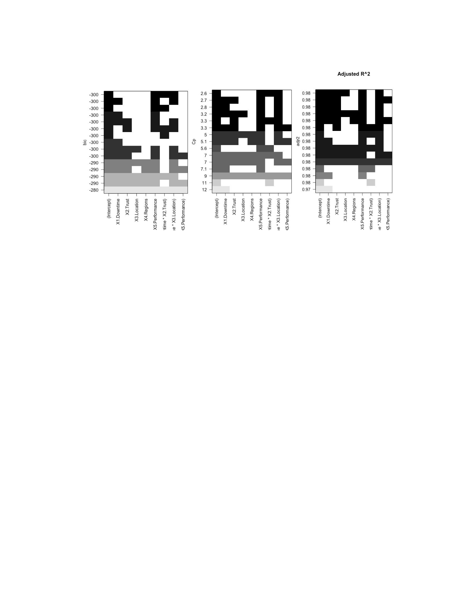
R: plot(regsubsets_out, scale = "adjr2", main = "Adjusted R^2") (4.25)
Figure 4-17 Best subset variable selection for Multiple Regression (Modified)
For the modified multiple linear regression model, I solved for the following equation
(Equation 4.26) using the R lm function (Equation 4.27) to fit the linear model based on
Least Squares with the transformed predictor variables. The output (Figure 4-18) from the
R summary (Equation 4.28) was presented and analyzed in the following section.
Y.Availability = B0 + B1 * X5.Performance + B2 * (X1.Downtime * X2.Trust) + B3 *
(X1.Downtime * X3.Location) + B4 * (X1.Downtime * X3.Location)2 (4.26)
R: MultModelExclude = lm(Y.Availability ~ X5.Performance + I(X1.Downtime * X2.Trust)
+ poly(X1.Downtime * X3.Location, degree=2, raw=TRUE),
data=MultDataExclude) (4.27)
4.3.2.3.1 Multiple Regression Model Summary
The modified linear regression model output in Figure 4-18 (based on the R summary
function Equation 4.28) was analyzed below.
R: summary(MultModelExclude,4) (4.28)
128
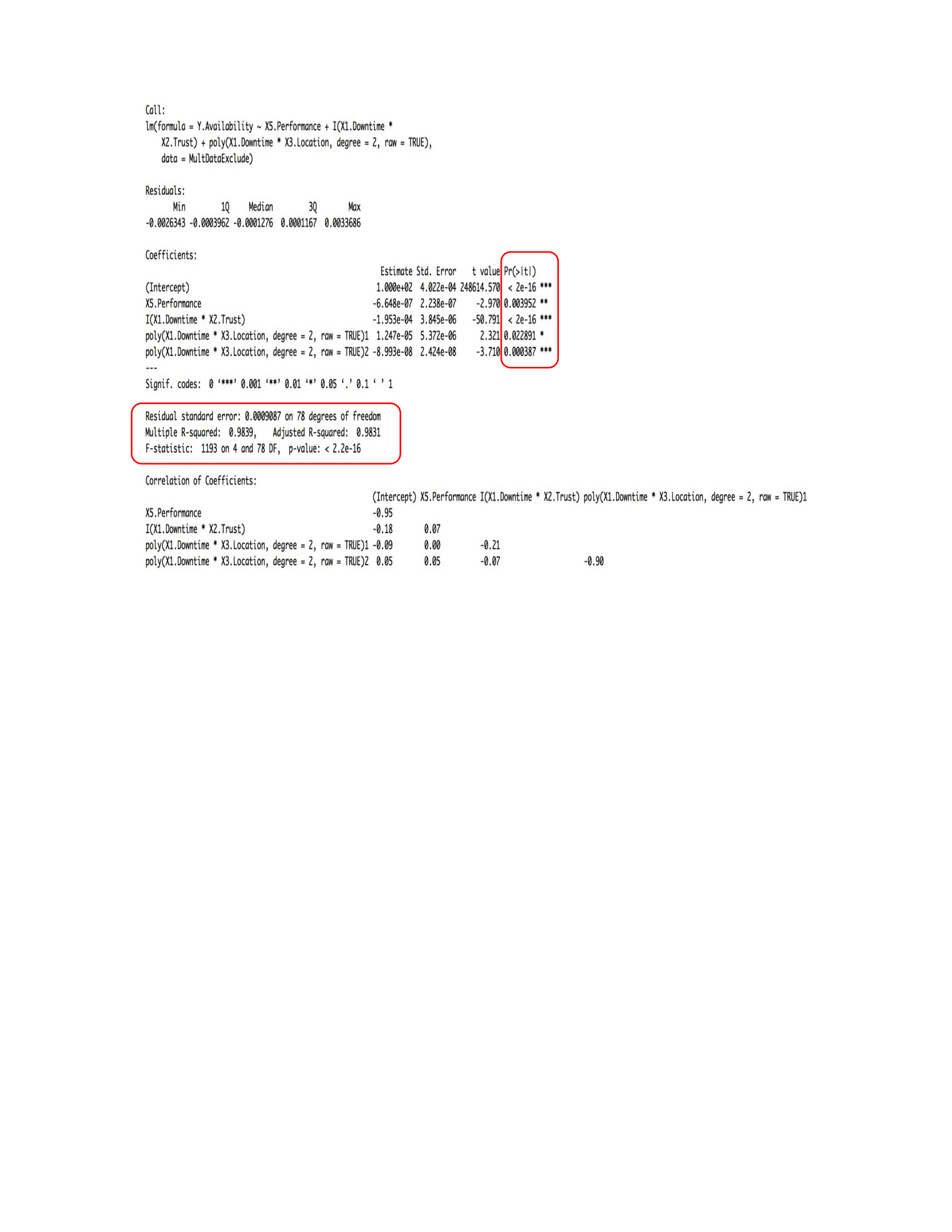
Figure 4-18 Multiple Regression Summary (Modified)
From the Figure 4-18 model summary output (see red circle) and the variable
scatterplot (Figure 4-16) we can make the following observations.
•The p-value, an overall test of the statistical significance for the model, is very
close to zero and the model produced a strong R-squared.
•The R-squared we get is 0.9839 (adjusted 0.9831), which is a high score. This
suggests the linear model we just fit in the data is explaining 98% of the variance
observed in the data.
•Looking at the coefficients, we can observe the dynamics related with response
variable Availability as we plug in the coefficient values into the regression
equation to get predicted Availability values. The p-values for each predictor are <
0.05, so we can say they are significant.
129

•The residual standard error, which measures the average amount of Availability
that will deviate from the true regression line for any given point, is 0.0009087.
This means that in the model, any prediction of Availability on the basis of the
predictor variables will be off by an average of 0.0009087, which is a small
number.
•Given that the residual standard error for Availability is 0.0009087 and the mean
Availability value is 1.000e+02 (Intercept), we can assume that the average
percentage error for any given point is 0.0009087% (0.0009087/1.000e+02 =
9.087e-06). Again, a small error rate (Tattar, Ramaiah, and Manjunath 2016,
Chatterjee and Hadi 2013).
4.3.2.3.2 ANOVA of Multiple Regression Model
We can analyze the ANOVA results (Table 4-10) related to the model using the R
anova function (Equation 4.29).
R: anova(MultModel) (4.29)
Looking at the following table (Table 4-10), we check the ANOVA F-test results to
confirm a linear relationship exists between Availability and the predictor variables. The
F value column contains F-test statistics and the Pr(>F) column contains the P-value
associated with the F-tests. The F-tests tells us “there is enough statistical evidence to
conclude a linear relationship exists” between Availability and the predictor variables
(Tattar, Ramaiah, and Manjunath 2016). The Regression Sum of Squares column
quantifies “how far the estimated regression line is from the no relationship line” (i.e. a
horizontal line) (Tattar, Ramaiah, and Manjunath 2016). The Residuals (Error) Sum of
Squares (= 6.44E-05), represents “how much the observed data points vary around
estimated regression line” (Tattar, Ramaiah, and Manjunath 2016). The total variation
130
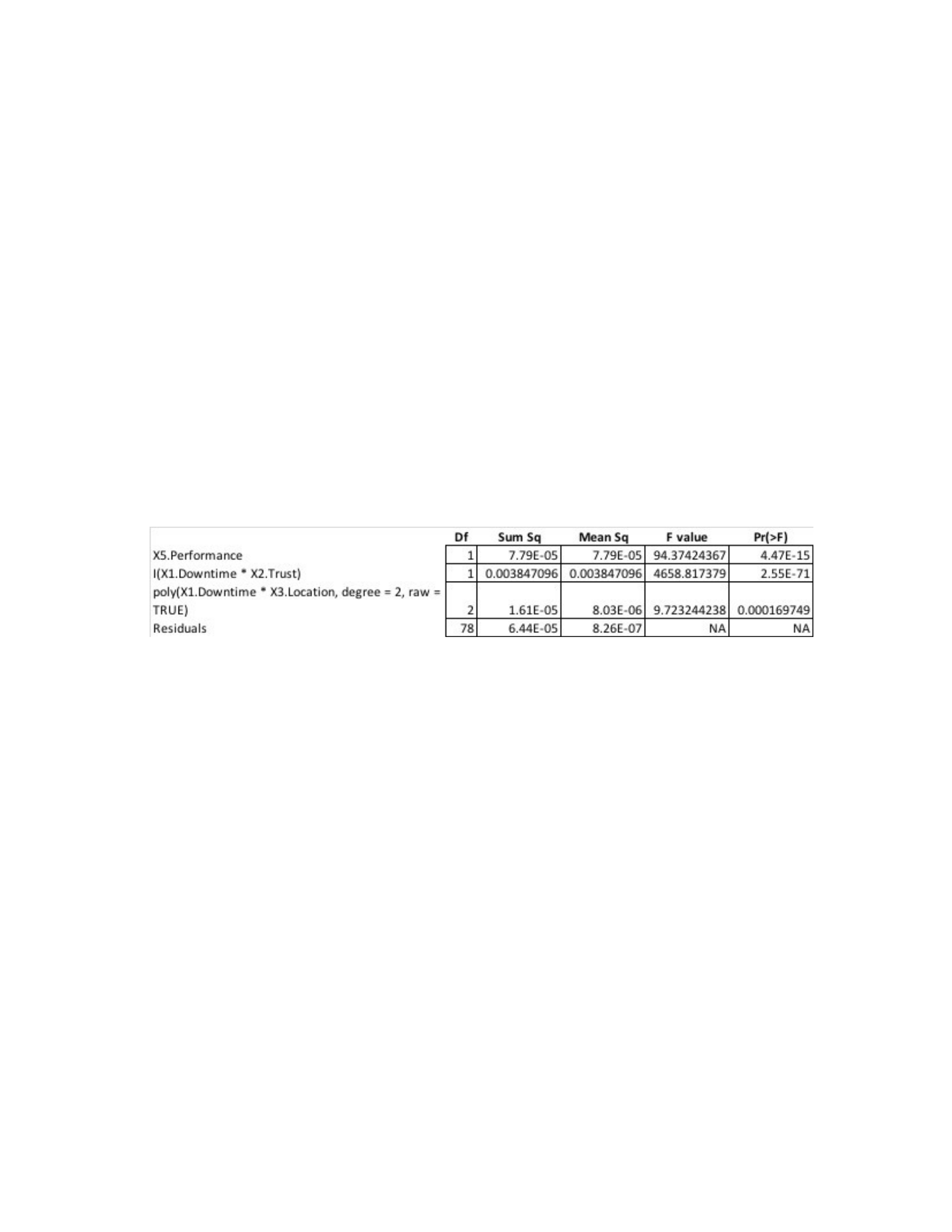
related to observed Availability is the sum of the column (i.e. variation due to all
predictors = 7.79E-05+0.003847096+1.61E-05 and variation due to random error =
6.44E-05). From the analysis, we can conclude the predictor variables were associated
with Availability and there was a linear association since the predictor variable’s
“Regression Sum of Squares [was] the larger component of the total sum of squares”
(Tattar, Ramaiah, and Manjunath 2016). We can also conclude that most of the variation
related to observed Availability data points were attributed to the predictor variables vs
“random error,” which is what we are looking for (Tattar, Ramaiah, and Manjunath
2016).
Table 4-10 ANOVA of Multiple Regression Model (Modified)
4.3.2.3.3 Multiple Regression Model Assumptions
To further assess the linear regression model and the relationship between
Availability and the predictor variables, compliance with key assumptions (as previously
introduced in the chapter 3 Methodology) related to Linearity, Normality, Independence,
Homoscedasticity, and Outliers is analyzed and presented in Appendix K (Fox 1991,
Chatterjee and Hadi 2013, Tattar, Ramaiah, and Manjunath 2016).
4.3.3 Linear Regression based Predictions (Simple vs Multiple)
The predictions related to the simple and multiple linear regression models leveraged
the following R related functions (Equation 4.30, 4.31) as expressed below by R:.
R: predict(SimpleModelExclude, newdata = SimpleTestData) (4.30)
R: predict(MultModelExclude, newdata = MultTestData) (4.31)
131
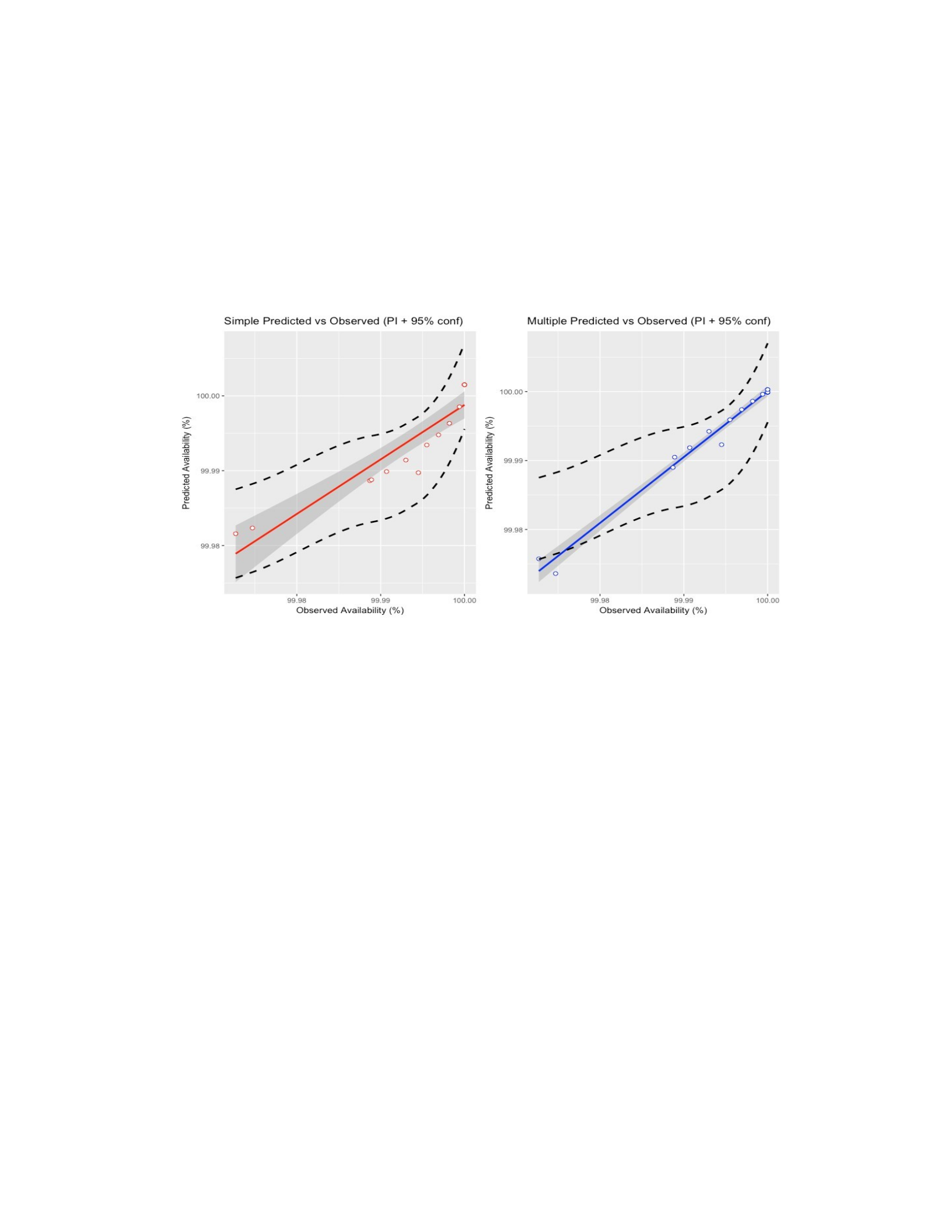
The diagrams below (Figure 4-19) provide visualizations for the simple and multiple
linear regression models. The following two diagrams present the regression line with
95% confidence interval in grey and 95% prediction interval (black dotted line) for both
the simple and multiple regression models. As you can see, the multiple regression
provides a better fit which is also reinforced by data in the following sections.
Figure 4-19 Predicted availability % vs observed, with PI and 95% CI (Simple, Multiple)
For comparison and contrast, the following diagram (Figure 4-20) on the left presents
the observed availability % and downtime minutes (black solid line) vs the multiple
regression (blue solid line) and simple regression (red dotted line). We can see the
improved fit for the multiple regression line. The diagram (Figure 4-20) on the right
provides a visualization of the predicted vs observed availability percentage between the
multiple linear regression and simple linear regression.
132
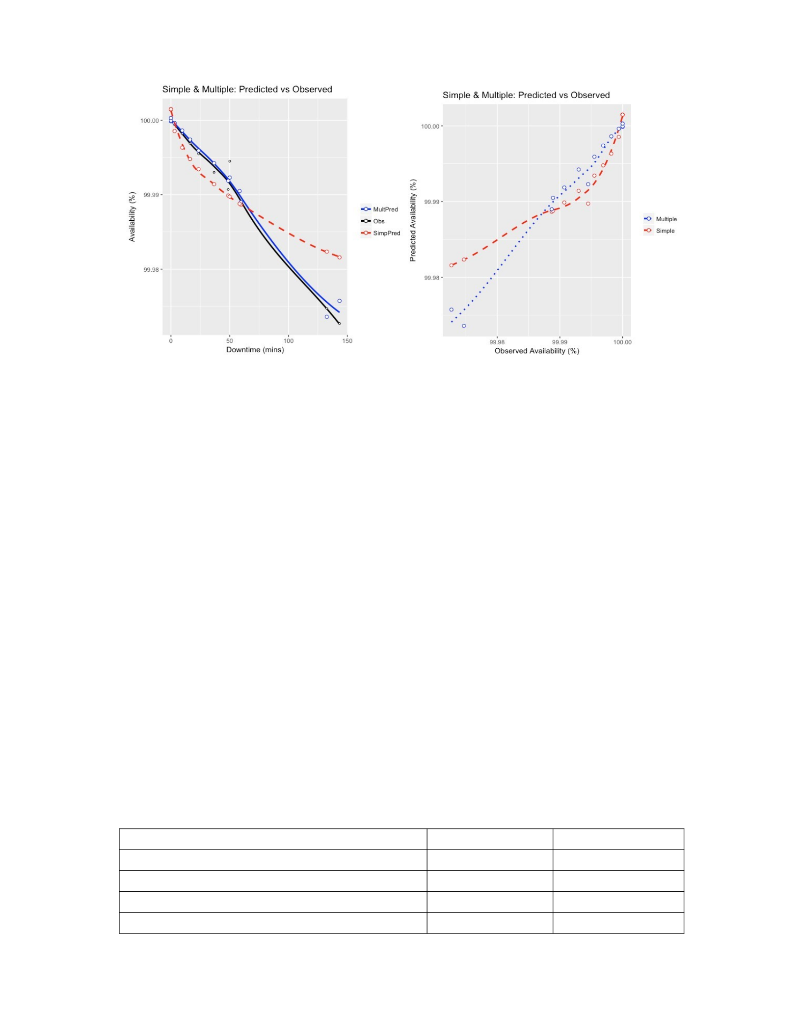
Figure 4-20 Simple and Multiple Availability % (predicted vs observed)
4.3.4 Comparing Linear Regression Models (Simple vs Multiple)
Predictions were performed for both models with multiple prediction intervals
between 50% and 95% using 5% increments. The results are summarized in section
4.3.4.3. Section 4.3.4.3 also presents a detailed example that illustrates and validates the
actual observed availability % values contrasted against the 95% prediction interval along
with the associated Fitted values and Standard Error.
4.3.4.1 Goodness of Fit of Simple and Multiple Regression Models
The following table (Table 4-11) presents multiple Goodness of Fit measures for the
simple and multiple linear regression models. The measures were calculated (via R
related functions in Appendix F) and analyzed to test the accuracy and quality of the fit
between the simple and multiple linear regression models.
Table 4-11 Linear Regression Model Measurements (simple and multiple modified)
Measurement Simple Multiple
Residual Standard Error 0.0029 0.0009
R.Squared 0.8113 0.9839
Adjusted.R.Squared 0.8089 0.9831
Predicted.R.Squared 0.7927 0.9806
133
Predictve Residual Sum of Squares (PRESS) 7.2290e-04 7.7646e-05
Akaike's An Information Criterion (AIC) -733.29 -920.19
Bayesian Information Criterion (BIC) -726.03 -905.68
Mallow's Cp 2 5
Root mean squared error (RMSE) 0.0034 0.0010
Mean Absolute Error (MAE) 0.0024 0.0007
Ratio of RMSE (RSR) 0.5031 0.1582
The quantity (Equation 4.32) from the R: expression exp((AICmin−AICi)/2)
represents the probability that model AICi will reduce information loss. The multiple
regression model is 2.601241e-41times more probable as the simple regression model to
minimize the information loss.
R: exp((-920.19 - (-733.29)) / 2) = 2.601241e-41 (4.32)
4.3.4.2 ANOVA of Simple and Multiple Regression Models
The ANOVA analysis (Table 4-12) comparing the simple and multiple linear
regression models leveraged the following R related function as expressed below by R:
(Equation 4.33). ANOVA is used to compare the models and measure what the multiple
linear regression added to the linear prediction above and beyond the simple linear
regression model.
R: anova(SimpleModelExclude, MultModelExclude) (4.33)
Table 4-12 ANOVA of Simple and Multiple Regression Models (Modified)
With the conventional test, we are compared the regression sums of squares for
the two models (i.e. extra sum of squares test). The null hypothesis that “additional
134

predictors all have zero coefficients” was tested using the F-statistics (Tattar, Ramaiah,
and Manjunath 2016). The “extra sum of squares” was the “amount by which the residual
sum of squares [was] reduced by the additional predictors” (Tattar, Ramaiah, and
Manjunath 2016). From the table (Table 4-12), we have: 0.00065811 – 0.00006179 =
0.00059632 (which is the Sum of Squares column). With a p-value = 2.2E-16 (which is
essentially 0 and is therefore < 0.05), we can reject the null hypothesis that the models are
the same. Since p-value is < 0.05, the models differ, so the added predictors do account
for enough variance (and have explanatory and predictive power).
4.3.4.3 Validating Simple and Multiple Linear Regression Models
Looking at the Table 4-13, the table checks the box for which predictor variables
(since the models are essentially nested) were used by the final simple and multiple
regression models; then checks the box for which Goodness of Fit measures supported
which model. Again, the data used to validate was actual data from and verified against
actual cloud service provider (CSP) performance. Based on the measurements and
validation, the Multiple Linear Regression Model represented an increased Goodness of
Fit over the Simple model.
Table 4-13 Goodness of Fit Measures and Validation
Model and
Response
Variable
Predictor Variables Measurements
Simple:
Availability
X -
Multiple:
Availability
X X X - X X X X X X X X X X X X
135
Downtime
Trust
Location
Regions
Performance
RSE
R-Squared
Adj R-Squared
Predicted R-Sq
PRESS
AIC
BIC
RMSE
MAE
RSR
ANOVA

As previously noted, there were 101 observations of which 15% were randomly used
to test and validate the models. The accuracy of the 15% were confirmed and validated
with actual CSP performance. The following scenarios compare, contrast and validate the
two models.
For the simple regression model, Table 4-14 row 6 (circled in red) illustrates a
downtime of 59.52 minutes (transformed with square root which was 7.7149), with the
actual availability of 99.9887%. This is within the 95% PI. The PI lower limit illustrates
the minimum availability % which could be as low as 99.98290%. The fitted availability
was 99.98834%.
For the multiple regression model, Table 4-15 row 6 (circled in blue) illustrates a
performance of 1066 (which represents latency and throughput values), plus the
interaction of downtime and trust level which is 54.83578 (59.92 minutes * 89.13% trust),
plus the transformed downtime per location of data centers (using polynomial of degree 2
for 59.92 minutes * 2 which represents APAC location) which is 32062.2336, with the
actual availability of 99.9887%. This is within the 95% PI. The PI lower limit depicts the
minimum availability % which could be as low as 99.99240%. The fitted availability is
99.98899%.
With respect to how the model will be used, both the lower and upper limits of the
percentile are relevant. Of course the lower is important in terms of expectations for cloud
service availability and the level of outages that are tolerated. The upper is important
from a financial perspective since the greater the maximum availability, the greater the
investment in capital (human, process and technology) to ensure the expected level of
availability.
136
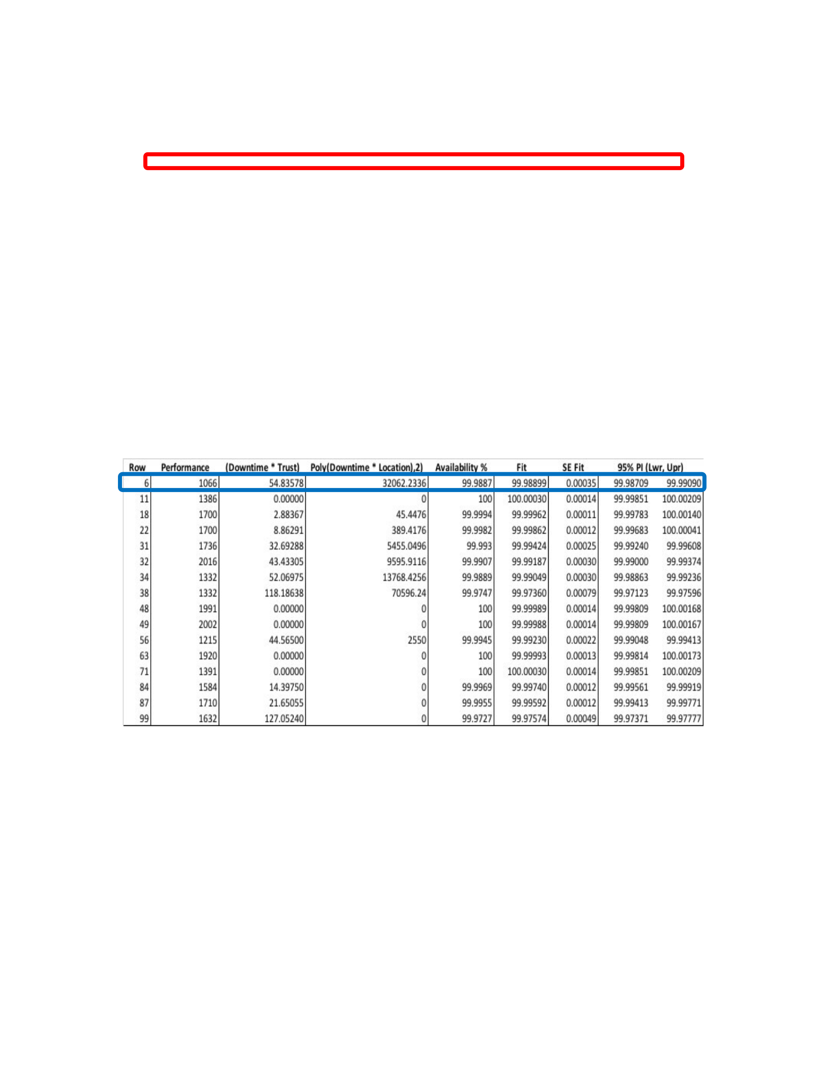
Table 4-14 Simple Linear Regression Model Predictions with 95% PI
Row SQRT(Downtime) Availability % Fit SE
Fit 95% PI (Lwr, Upr)
6 7.714920609 99.9887 99.98834 0.00052 99.98290 99.99443 11 0 100 100.00148 0.00042
99.99575 100.00721
18 1.769180601 99.9994 99.99854 0.00033 99.99283 100.00425
22 3.101612484 99.9982 99.99633 0.00031 99.99062 100.00203 31 6.056401572 99.993 99.99142
0.00041 99.98569 99.99715
32 6.980687645 99.9907 99.98988 0.00047 99.98414 99.99563
34 7.643297718 99.9889 99.98878 0.00051 99.98302 99.99454
38 11.51520734 99.9747 99.98235 0.00081 99.97645 99.98825 48 0 100 100.00148 0.00042
99.99575 100.00721
49 0 100 100.00148 0.00042 99.99575 100.00721
56 7.071067812 99.9945 99.98973 0.00047 99.98398 99.99548 63 0 100 100.00148 0.00042
99.99575 100.00721
71 0 100 100.00148 0.00042 99.99575 100.00721
84 4.031128874 99.9969 99.99478 0.00032 99.98907 100.00049 87 4.847679857 99.9955 99.99343
0.00035 99.98771 99.99914
99 11.9749739 99.9727 99.98159 0.00085 99.97567 99.98750
Table 4-15 Multiple Linear Regression Model Predictions with 95% PI
Chapter 5. Conclusion
A number of drivers (e.g. security, scalability, financial) are influencing the move of
applications to cloud infrastructure (Skyhigh 2017). However, challenges exist such as
complexity and lack of expertise, governance and management of multiple cloud services
137

(RightScale 2017a). As cloud usage increases, so does the potential impact to service
levels and financial risk (Ponemon 2017).
Effective management of service levels (e.g. availability, reliability, performance,
security) and financial risk to cloud service customers (CSCs) is dependent on the cloud
service provider’s (CSP’s) capability and trustworthiness. Cloud service level agreements
(SLAs) and a model for assessing, predicting and governing compliance of cloud services
and service levels is required. Industry efforts are underway to standardize cloud SLAs
(EC 2014, Hunnebeck et al. 2011, ISO/IEC 2016, NIST 2015, Hogben, Giles and Dekker
2012) and examine frameworks for assessing CSP trustworthiness (Ghosh, Ghosh and
Das 2015, Taha et al. 2014).
The primary objective of this research study was to analyze cloud SLAs and cloud
security requirements, assess and define CSP trustworthiness levels, and establish a
model for predicting cloud SLA availability based on multiple factors (e.g. CSP trust
levels, cloud service historic performance and cloud service characteristics). The research
study focused on leveraging and extending existing research related to the lifecycle of
cloud SLAs and CSP trust models. The methodologies used included Graph Theory to
analyze cloud SLAs and cloud security, Analytic Hierarchy Process (AHP) to assess CSP
trustworthiness, and Linear Regression Analysis to build predictive models for cloud
SLA performance based on output from the other methodologies.
5.1 Hypothesis Results and Model Validation
For this research, the hypothesis asserted that SLA based cloud service availability
could be calculated with greater accuracy when based on additional criteria besides
merely historical downtime. The other criteria considered included CSP trustworthiness,
138

global cloud service locations, cloud service capacity and cloud service performance. The
following hypothesis was proposed and tested:
Predicting SLA-based cloud service availability has greater accuracy when
calculated with more criteria than just historical cloud service downtime (e.g. CSP
trustworthiness; global cloud service locations, resource capacity and performance).
To test the hypothesis, a null hypothesis was defined that proposed a simple linear
regression model, with a single regression coefficient for cloud service downtime, had
zero difference in accuracy to a multiple linear regression model, incorporating multiple
regression coefficients (the variables are defined in Table N-1). In other words, the
hypothesis asserted that no additional variables besides cloud service downtime offered
explanatory or predictive power to the linear regression model. The alternative hypothesis
stated that at least one additional variable provided statistically significant contribution to
explaining cloud service availability and therefore should be in the model.
H0 : Multiple = Simple LR model, i.e. zero difference in accuracy (Bj = 0); no
additional variables have explanatory/predictive power (i.e. don’t contribute to
the Simple LR model).
Ha : At least one additional variable (Bj) has a statistically significant contribution
to explaining/predicting Y (Bj != 0), and therefore should remain in the model.
Based on the Goodness of Fit (from section 4.3.4.1), including ANOVA F-test results
comparing the multiple vs simple regression models (from section 4.3.4.2), and model
validation results (from section 4.3.4.3; and review of Figure 5-1, Tables 5-1 to 5-3), the
null hypothesis was rejected. The answer to the primary question was yes, predicting
cloud computing SLA availability performance does have greater accuracy when
139
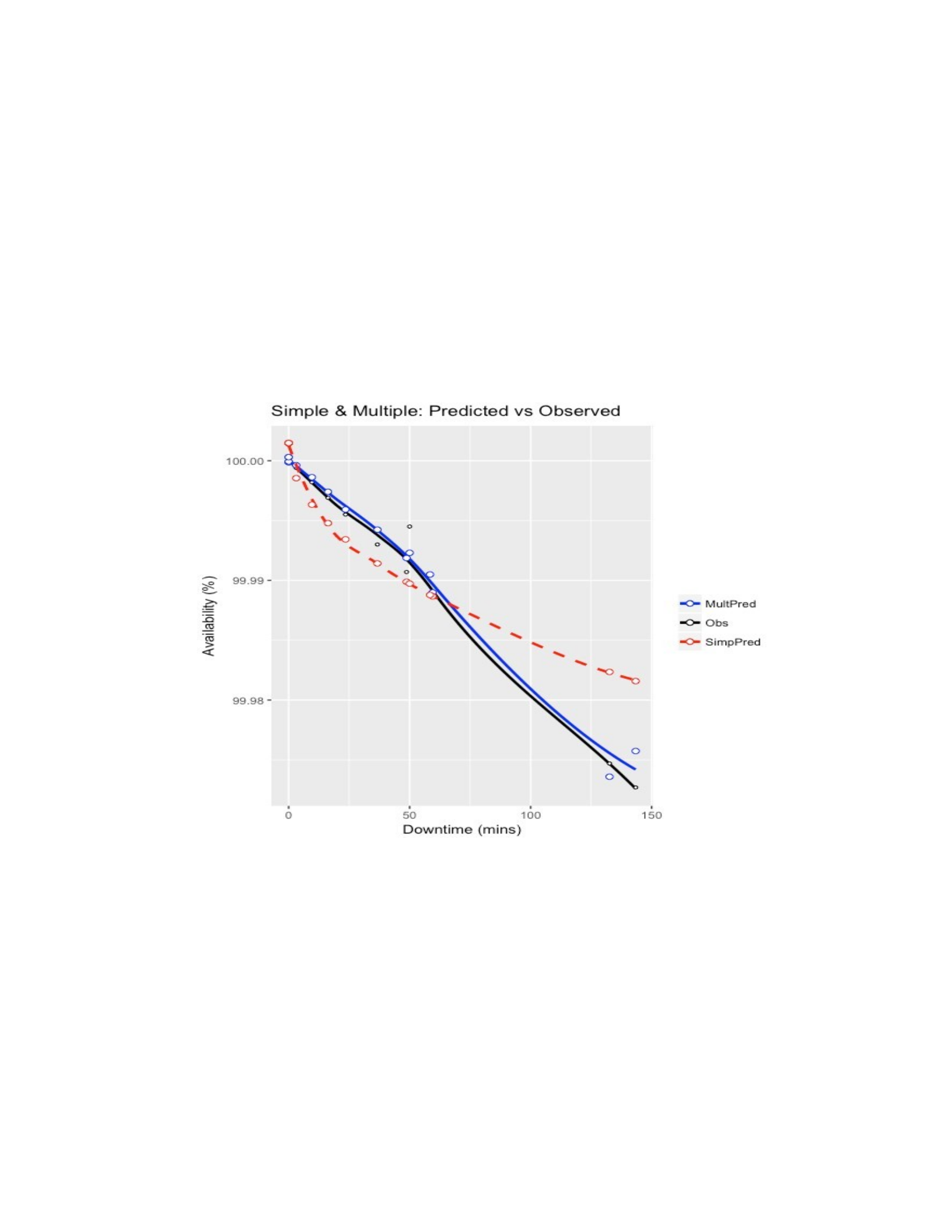
calculated with more predictor variables than just historical cloud service downtime. The
additional predictor variables included historical SLA performance, cloud service
performance, cloud service characteristics such as location and number of service regions,
and CSP trustworthiness.
Reviewing Figure 5-1, we can visualize and validate the improved fit of the multiple
regression model (blue solid line) vs the simple regression model (red dotted line),
against the observed (black line) availability % and downtime minutes.
Figure 5-1 Simple and Multiple Availability % (predicted vs observed)
Further validation is demonstrated by Table 5-1. The table checks the box for which
predictor variables (since the models are essentially nested) were used by the final simple
and multiple regression models; then checks the box for which Goodness of Fit measures
supported which model. Based on the measurements and validation, the Multiple Linear
Regression Model represented an increased Goodness of Fit over the Simple model.
140
Table 5-1 Goodness of Fit Measures and Validation
Model and
Response
Variable
Predictor Variables Measurements
Simple:
Availability
X -
Multiple:
Availability
X X X - X X X X X X X X X X X X
As previously reviewed (section 3.3.3.1), there were 101 observations of which 15%
were randomly used to test and validate the models. The accuracy of the 15% were
confirmed and validated against actual CSP performance. The following using Table 5-2
and 5-3, illustrates and validates the models with actual observed availability % values
contrasted against the 95% prediction intervals along with the associated Fitted values
and Standard Errors.
For the simple regression model, Table 5-2 row 6 (circled in red) illustrates a
downtime of 59.52 minutes (transformed with the square root which was 7.7149), with
the actual availability of 99.9887%. This is within the 95% PI. The PI lower limit
illustrates the minimum availability % which could be as low as 99.98290%. The fitted
availability was 99.98834%.
Table 5-2 Simple Linear Regression Model Predictions with 95% PI
Row SQRT(Downtime) Availability % Fit SE
Fit 95% PI (Lwr, Upr)
6 7.714920609 99.9887 99.98834 0.00052 99.98290 99.99443 11 0 100 100.00148 0.00042
99.99575 100.00721
18 1.769180601 99.9994 99.99854 0.00033 99.99283 100.00425
22 3.101612484 99.9982 99.99633 0.00031 99.99062 100.00203 31 6.056401572 99.993 99.99142
0.00041 99.98569 99.99715
32 6.980687645 99.9907 99.98988 0.00047 99.98414 99.99563
34 7.643297718 99.9889 99.98878 0.00051 99.98302 99.99454
141
Downtime
Trust
Location
Regions
Performance
RSE
R-Squared
Adj R -Squared
Predicted R-Sq
PRESS
AIC
BIC
RMSE
MAE
RSR
ANOVA
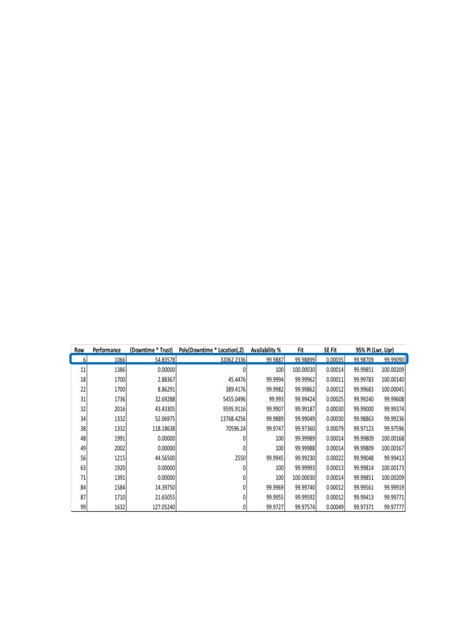
38 11.51520734 99.9747 99.98235 0.00081 99.97645 99.98825 48 0 100 100.00148 0.00042
99.99575 100.00721
49 0 100 100.00148 0.00042 99.99575 100.00721
56 7.071067812 99.9945 99.98973 0.00047 99.98398 99.99548 63 0 100 100.00148 0.00042
99.99575 100.00721
71 0 100 100.00148 0.00042 99.99575 100.00721
84 4.031128874 99.9969 99.99478 0.00032 99.98907 100.00049 87 4.847679857 99.9955 99.99343
0.00035 99.98771 99.99914
99 11.9749739 99.9727 99.98159 0.00085 99.97567 99.98750
For the multiple regression model, Table 5-3 row 6 (same observation circled in blue)
illustrates a performance of 1066 (which represents latency and throughput values), plus
the interaction of downtime and trust level which is 54.83578 (59.92 minutes * 89.13%
trust), plus the transformed downtime per location of data centers (using polynomial of
degree 2 for 59.92 minutes * 2 which represents APAC location) which is 32062.2336,
with the actual availability of 99.9887%. This is within the 95% PI. The PI lower limit
depicts the minimum availability % which could be as low as 99.99240%. The fitted
availability is 99.98899%.
Table 5-3 Multiple Linear Regression Model Predictions with 95% PI
With respect to how the model will be used (reviewed in section 5.2), both the lower
and upper limits of the percentile are relevant. Of course the lower is important in terms
142

of expectations for cloud service availability and the level of outages that are tolerated.
The upper is important from a financial perspective since the greater the maximum
availability, the greater the investment in capital (human, process and technology) to
ensure the expected level of availability.
5.2 Applications for the Research and Predictive Models
Below are five high level scenarios depicting how results of this research study and
the predictive model could be applied. Organizations can utilize the model to:
•Predict and set expectations concerning quality of cloud computing services.
•Identify required levels of investment (both capital and expense) to support the
required quality of cloud computing service.
•Identify continuous improvement programs to enhance cloud computing service
capabilities and compliance with respect to cloud SLAs and industry regulations
(e.g. security, delivery and support, performance, reliability, business continuity).
•Identify opportunities to right size cloud computing service capabilities based on
financial drivers, competitive market conditions, and/or customer requirements.
•Evaluate and select cloud service providers or compare and contrast private vs
public cloud computing services.
Related to the scenarios above, organizations (for example cloud service customers or
cloud service providers) can specify the required prediction intervals to drive required
values of corresponding predictor variables which ultimately ensure predictions remain
within the expected prediction interval. This reflects a reverse engineering exercise that
reconciles the required capabilities and security in support of the required prediction
interval. The required predictor variable values can provide visibility and awareness to
143

the required cloud service capabilities and budgets (i.e. traceability and transparency from
expectations to the required investment levels and cloud service capabilities that satisfy
requirements). The predictive model can apply to both public cloud and/or private cloud
scenarios (e.g. organizations that are comparing whether to utilize private vs public vs
hybrid; or organizations that are assessing the required investment to their internal private
cloud based on required cloud SLA availability levels).
To support the scenarios, the lower and upper limits of the predictor interval can be
used in a number of ways. For example:
•Since all CSPs have SLA Availability compliance levels with financial
consequence (e.g. Amazon >= 99.99%, Google and Microsoft >= 99.95%), their
SLA levels can serve to influence the required prediction intervals (PIs). The
model can serve to ensure proactive and predictive alignment and delivery against
those SLA availability levels (SLA AWS 2017, SLA Google 2017, SLA Microsoft
2017).
•Lower limit of the PI can establish a minimum Availability % expectation,
resulting in re-engineering cloud service capabilities to ensure performance at the
required level. This application could assist CSPs with mitigating under delivery.
•Conversely, the upper limit of the PI can establish a maximum Availability %
expectation, which can drive refactoring and right sizing of cloud service
capabilities to meet required performance levels. This application could assist
CSPs with managing over delivery and over investment.
144

•Cloud service customers (CSCs) and cloud service providers (CSPs) can apply the
model and required PIs to drive business continuity plans and service targets such
as recovery time objectives (RTOs) and recovery point objectives (RPOs).
Additional scenarios introduce how predictor variables such as CSP trustworthiness
levels can be managed. The trust levels (as calculated by AHP analysis in section 4.2) are
based on the level of sophistication and compliance with industry cloud SLA standards
and security frameworks. The higher the trust level, the more capability, security and
compliance with frameworks such as Cloud Security Alliance Cloud Controls Matrix and
their requirements related controls (CSA CCM 2017, CSA CAIQ 2017). At the same
time, a cloud service provide has to ask how good do they need to be – what is the
required level capability to be competitive and satisfy customer requirements. This can
vary depending on how the cloud compute service is going to be used … multiple service
levels can exist. So depending on the required PI level, predictors variables can be
managed based on service levels, CSC requirements and instances of cloud compute
services.
The same analysis and management can apply to other predictors in the model. For
example, what level of cloud performance regarding latency and throughput is required,
and/or how many CSP service regions are required within each global location, to satisfy
required service levels.
5.3 Future Research Opportunities
A number of future research opportunities exist related to the results of this research
study. Work within the cloud community continues to mature methods and standards for
managing cloud service levels, cloud SLAs and their adoption (Hunnebeck 2011,
145

ISO/IEC 2016, NIST 2015, EC 2014). This research study organized and analyzed the
work around four phases of a cloud SLA lifecycle.
The first phase focused on cloud SLA specifications, their importance, benefits,
standards and frameworks. The work is not complete and continues across both
international standards bodies, industry organizations and CSPs. Opportunities exist for
continuing future analysis concerning the diversity of CSP SLAs, adoption of cloud SLA
standards and methods for verifying compliance along with automation for predictive and
proactive cloud SLA management across the other phases of the lifecycle.
The second phase of the cloud SLA lifecycle focused on CSP trustworthiness models
based on CSP capabilities (e.g. CSA CCM), transparency and historical performance.
Over the past few years, research focused on CSP trustworthiness, specifically related to
security. Additional opportunities exist with respect to correlating CSP capabilities and
compliance (e.g. CSA CCM) with CSP historical SLA performance, CSC experience and
satisfaction levels, and other service level and delivery characteristics (e.g. adoption and
transparency against cloud SLA standards).
The third phase of the cloud SLA lifecycle focused on monitoring cloud services, CSP
trust levels, and quality of the services with respect to SLA compliance. Maintaining a
service level context and real-time focus with respect to monitoring CSP trust levels and
the relationship with cloud services and cloud SLAs is an opportunity for further work
related to predictive models. Predictive identification of quantitative and qualitative
service level risk based on the monitoring could offer proactive mitigation measures to
CSPs and CSCs.
The last phase of the cloud SLA lifecycle, offered additional research opportunities
related to enforcement of proactive mitigation measures. There has been important work
146

from organizations such as IEEE and DMTF (Linthicum 2016, Diaz-Montes et al. 2016,
DMTF 2015, Ferry et al. 2013) associated with orchestration, containers, and autonomic
self-managing clouds. The opportunity for further research could direct this work toward
automated governance driving cloud SLA compliance and proactive mitigation of service
level risk based on the predictive model research from phase three.
147

