Enabling Persistence Using a Real-World Application

The completed storage engine is not intended for production use and does not

implement all the features a production quality storage engine should. We implement

only the basic functionality to demonstrate how to begin persistent memory

programming using a well known database. The intent is to provide you with a more

hands-on approach for persistent memory programming so you may enable persistent

memory features and functionality within your own application. Our storage engine is

left as an optional exercise for you to complete. Doing so would create a new persistent

memory storage engine for MariaDB, MySQL, Percona Server, and other derivatives. You

may also choose to modify an existing MySQL database storage engine to add persistent

memory features, or perhaps choose a different database entirely.

We assume that you are familiar with the preceding chapters that covered the

fundamentals of the persistent memory programming model and Persistent Memory

Development Kit (PMDK). In this chapter, we implement our storage engine using C++

and libpmemobj-cpp from Chapter 8. If you are not a C++ developer, you will still

find this information helpful because the fundamentals apply to other languages and

applications.

The complete source code for the persistent memory-aware database storage engine

can be found on GitHub at

https://github.com/pmem/pmdk-examples/tree/master/pmem-mariadb.

The Database Example

A tremendous number of existing applications can be categorized in many ways. For the

purpose of this chapter, we explore applications from the common components

perspective, including an interface, a business layer, and a store. The interface interacts

with the user, the business layer is a tier where the application’s logic is implemented,

and the store is where data is kept and processed by the application.

With so many applications available today, choosing one to include in this book that

would satisfy all or most of our requirements was difficult. We chose to use a database

as an example because a unified way of accessing data is a common denominator for

many applications.

Different Persistent Memory Enablement Approaches

The main advantages of persistent memory include:

It provides access latencies that are lower than flash SSDs.

It has higher throughput than NAND storage devices.

Real-time access to data allows ultrafast access to large datasets.

Data persists in memory after a power interruption.

Persistent memory can be used in a variety of ways to deliver lower latency for

many applications:

In-memory databases: In-memory databases can leverage persistent

memory’s larger capacities and significantly reduce restart times. Once the

database memory maps the index, tables, and other files, the data is

immediately accessible. This avoids lengthy startup times where the data is

traditionally read from disk and paged in to memory before it can be

accessed or processed.

Fraud detection: Financial institutions and insurance companies can

perform real-time data analytics on millions of records to detect fraudulent

transactions.

Cyber threat analysis: Companies can quickly detect and defend against

increasing cyber threats.

Web-scale personalization: Companies can tailor online user experiences

by returning relevant content and advertisements, resulting in higher user

click-through rate and more e-commerce revenue opportunities.

Financial trading: Financial trading applications can rapidly process and

execute financial transactions, allowing them to gain a competitive

advantage and create a higher revenue opportunity.

Internet of Things (IoT) : Faster data ingest and processing of huge

datasets in real-time reduces time to value.

Content delivery networks (CDN) : A CDN is a highly distributed network

of edge servers strategically placed across the globe with the purpose of

rapidly delivering digital content to users. With a memory capacity, each

CDN node can cache more data and reduce the total number of servers, while

networks can reliably deliver low-latency data to their clients. If the CDN

cache is persisted, a node can restart with a warm cache and sync only the

data it is missed while it was out of the cluster.

Developing a Persistent Memory-Aware MariaDB*

Storage Engine

The storage engine developed here is not production quality and does not implement all

the functionality expected by most database administrators. To demonstrate the

concepts described earlier, we kept the example simple, implementing table create(),

open(), and close() operations and INSERT, UPDATE, DELETE, and SELECT SQL

operations. Because the storage engine capabilities are quite limited without indexing,

we include a simple indexing system using volatile memory to provide faster access to

the data residing in persistent memory.

Although MariaDB has many storage engines to which we could add persistent

memory, we are building a new storage engine from scratch in this chapter. To learn

more about the MariaDB storage engine API and how storage engines work, we suggest

reading the MariaDB “Storage Engine Development” documentation

(https://mariadb.com/kb/en/library/storage-engines-storage-

engine-development/). Since MariaDB is based on MySQL, you can also refer to the

MySQL “Writing a Custom Storage Engine” documentation

(https://dev.mysql.com/doc/internals/en/custom-engine.html) to

find all the information for creating an engine from scratch.

Understanding the Storage Layer

MariaDB provides a pluggable architecture for storage engines that makes it easier to

develop and deploy new storage engines. A pluggable storage engine architecture also

makes it possible to create new storage engines and add them to a running MariaDB

server without recompiling the server itself. The storage engine provides data storage

and index management for MariaDB. The MariaDB server communicates with the

storage engines through a well-defined API.

In our code, we implement a prototype of a pluggable persistent memory–enabled

storage engine for MariaDB using the libpmemobj library from the Persistent

Memory Development Kit (PMDK).

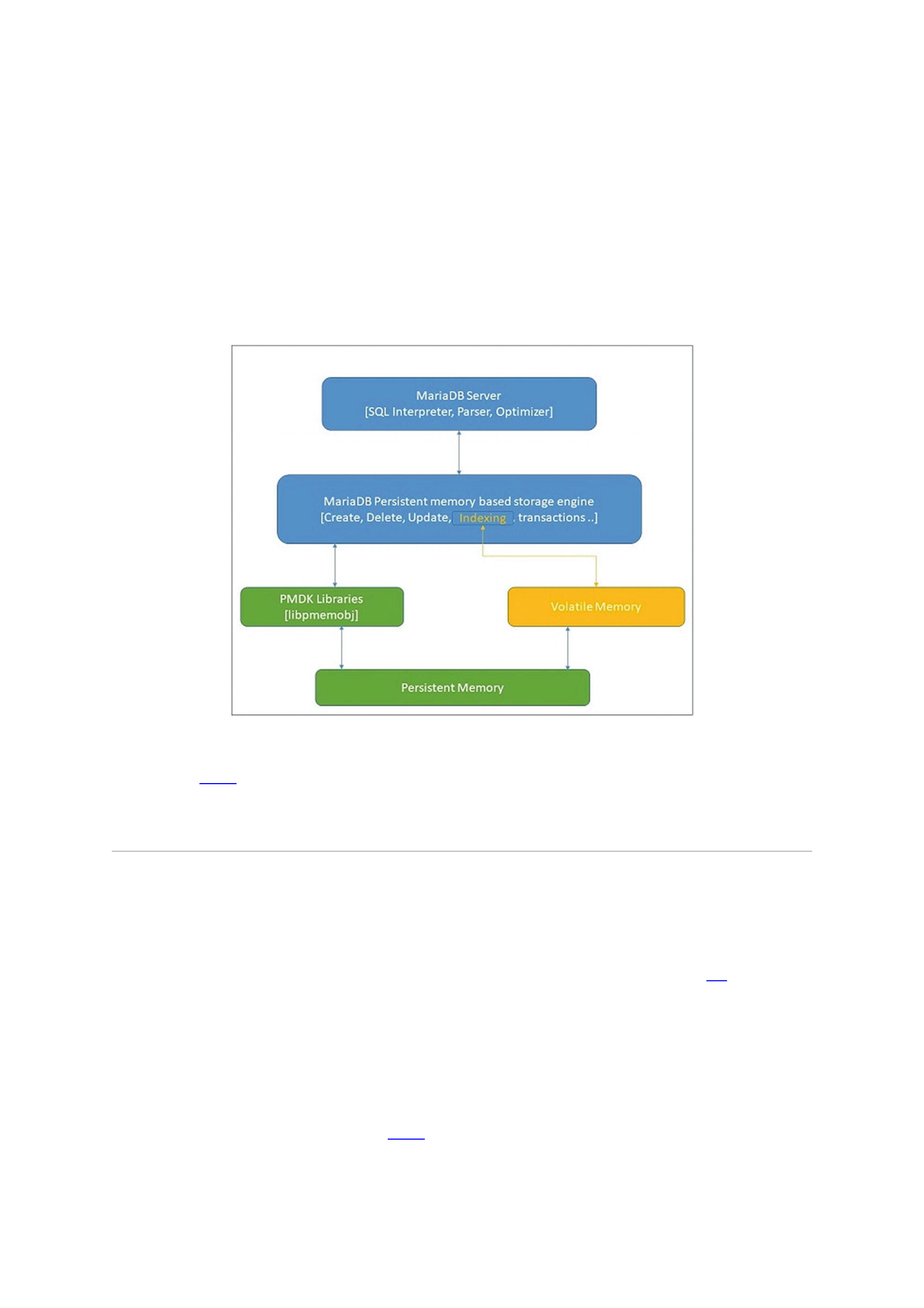
Figure 13-1MariaDB storage engine architecture diagram for persistent memory

Figure 13-1 shows how the storage engine communicates with libpmemobj to

manage the data stored in persistent memory. The library is used to turn a persistent

memory pool into a flexible object store.

Creating a Storage Engine Class

The implementation of the storage engine described here is single-threaded to support

a single session, a single user, and single table requests. A multi-threaded

implementation would detract from the focus of this chapter. Chapter 14 discussed

concurrency in more detail. The MariaDB server communicates with storage engines

through a well-defined handler interface that includes a handlerton, which is a

singleton handler that is connected to a table handler. The handlerton defines the

storage engine and contains pointers to the methods that apply to the persistent

memory storage engine.

The first method the storage engine needs to support is to enable the call for a new

handler instance, shown in Listing 13-1.

117 static handler *pmdk_create_handler(handlerton *hton,

118 TABLE_SHARE *table,

119 MEM_ROOT *mem_root);

120

121 handlerton *pmdk_hton;

Listing 13-1ha_pmdk.cc – Creating a new handler instance

When a handler instance is created, the MariaDB server sends commands to the

handler to perform data storage and retrieve tasks such as opening a table,

manipulating rows, managing indexes, and transactions. When a handler is

instantiated, the first required operation is the opening of a table. Since the storage

engine is a single user and single-threaded implementation, only one handler instance

is created.

Various handler methods are also implemented; they apply to the storage engine

as a whole, as opposed to methods like create() and open() that work on a per-

table basis. Some examples of such methods include transaction methods to handle

commits and rollbacks, shown in Listing 13-2.

209 static int pmdk_init_func(void *p)

210 {

...

213 pmdk_hton= (handlerton *)p;

214 pmdk_hton->state= SHOW_OPTION_YES;

215 pmdk_hton->create= pmdk_create_handler;

216 pmdk_hton->flags= HTON_CAN_RECREATE;

217 pmdk_hton->tablefile_extensions= ha_pmdk_exts;

218

219 pmdk_hton->commit= pmdk_commit;

220 pmdk_hton->rollback= pmdk_rollback;

...

223 }

Listing 13-2ha_pmdk.cc – Handler methods including transactions, rollback, etc

The abstract methods defined in the handler class are implemented to work with

persistent memory. An internal representation of the objects in persistent memory is

created using a single linked list (SLL). This internal representation is very helpful to

iterate through the records to improve performance.

To perform a variety of operations and gain faster and easier access to data, we used

the simple row structure shown in Listing 13-3 to hold the pointer to persistent

memory and the associated field value in the buffer.

71 struct row {

72 persistent_ptr<row> next;

73 uchar buf[];

74 };

Listing 13-3ha_pmdk.h – A simple data structure to store data in a single linked list

Creating a Database Table

The create() method is used to create the table. This method creates all necessary

files in persistent memory using libpmemobj. As shown in Listing 13-4, we create a

new pmemobj type pool for each table using the pmemobj_create() method ; this

method creates a transactional object store with the given total poolsize. The table is

created in the form of an .obj extension.

1247 int ha_pmdk::create(const char *name, TABLE *table_arg,

1248 HA_CREATE_INFO *create_info)

1249 {

1250

1251 char path[MAX_PATH_LEN];

1252 DBUG_ENTER("ha_pmdk::create");

1253 DBUG_PRINT("info", ("create"));

1254

1255 snprintf(path, MAX_PATH_LEN, "%s%s", name, PMEMOBJ_EXT);

1256 PMEMobjpool *pop = pmemobj_create(path,

name,PMEMOBJ_MIN_POOL, S_IRWXU);

1257 if (pop == NULL) {

1258 DBUG_PRINT("info", ("failed : %s error number :

%d",path,errCodeMap[errno]));

1259 DBUG_RETURN(errCodeMap[errno]);

1260 }

1261 DBUG_PRINT("info", ("Success"));

1262 pmemobj_close(pop);

1263

1264 DBUG_RETURN(0);

1265 }

Listing 13-4Creating a table method

Opening a Database Table

Before any read or write operations are performed on a table, the MariaDB server calls

the open()method to open the data and index tables. This method opens all the named

tables associated with the persistent memory storage engine at the time the storage

engine starts. A new table class variable, objtab, was added to hold the

PMEMobjpool. The names for the tables to be opened are provided by the MariaDB

server. The index container in volatile memory is populated using the open() function

call at the time of server start using the

loadIndexTableFromPersistentMemory() function .

The pmemobj_open() function from libpmemobj is used to open an existing

object store memory pool (see Listing 13-5). The table is also opened at the time of a

table creation if any read/write action is triggered.

290 int ha_pmdk::open(const char *name, int mode, uint

test_if_locked)

291 {

...

302 objtab = pmemobj_open(path, name);

303 if (objtab == NULL)

304 DBUG_RETURN(errCodeMap[errno]);

305

306 proot = pmemobj_root(objtab, sizeof (root));

307 // update the MAP when start occured

308 loadIndexTableFromPersistentMemory();

...

310 }

Listing 13-5ha_pmdk.cc – Opening a database table

Once the storage engine is up and running, we can begin to insert data into it. But we

first must implement the INSERT, UPDATE, DELETE, and SELECT operations.

Closing a Database Table

When the server is finished working with a table, it calls the closeTable() method

to close the file using pmemobj_close() and release any other resources (see Listing

13-6). The pmemobj_close() function closes the memory pool indicated by objtab

and deletes the memory pool handle.

376 int ha_pmdk::close(void)

377 {

378 DBUG_ENTER("ha_pmdk::close");

379 DBUG_PRINT("info", ("close"));

380

381 pmemobj_close(objtab);

382 objtab = NULL;

383

384 DBUG_RETURN(0);

385 }

Listing 13-6ha_pmdk.cc – Closing a database table

INSERT Operation

The INSERT operation is implemented in the write_row() method , shown in Listing

13-7. During an INSERT, the row objects are maintained in a singly linked list. If the

table is indexed, the index table container in volatile memory is updated with the new

row objects after the persistent operation completes successfully. write_row() is an

important method because, in addition to the allocation of persistent pool storage to the

rows, it is used to populate the indexing containers. pmemobj_tx_alloc() is used for

inserts. write_row() transactionally allocates a new object of a given size and

type_num.

417 int ha_pmdk::write_row(uchar *buf)

418 {

...

421 int err = 0;

422

423 if (isPrimaryKey() == true)

424 DBUG_RETURN(HA_ERR_FOUND_DUPP_KEY);

425

426 persistent_ptr<row> row;

427 TX_BEGIN(objtab) {

428 row = pmemobj_tx_alloc(sizeof (row) + table->s->reclength,

0);

429 memcpy(row->buf, buf, table->s->reclength);

430 row->next = proot->rows;

431 proot->rows = row;

432 } TX_ONABORT {

433 DBUG_PRINT("info", ("write_row_abort errno :%d ",errno));

434 err = errno;

435 } TX_END

436 stats.records++;

437

438 for (Field **field = table->field; *field; field++) {

439 if ((*field)->key_start.to_ulonglong() >= 1) {

440 std::string convertedKey =

IdentifyTypeAndConvertToString((*field)->ptr, (*field)-

>type(),(*field)->key_length(),1);

441 insertRowIntoIndexTable(*field, convertedKey, row);

442 }

443 }

444 DBUG_RETURN(err);

445 }

Listing 13-7ha_pmdk.cc – Closing a database table

In every INSERT operation , the field values are checked for a preexisting duplicate.

The primary key field in the table is checked using the isPrimaryKey()function (line

423). If the key is a duplicate, the error HA_ERR_FOUND_DUPP_KEY is returned. The

isPrimaryKey() is implemented in Listing 13-8.

462 bool ha_pmdk::isPrimaryKey(void)

463 {

464 bool ret = false;

465 database *db = database::getInstance();

466 table_ *tab;

467 key *k;

468 for (unsigned int i= 0; i < table->s->keys; i++) {

469 KEY* key_info = &table->key_info[i];

470 if (memcmp("PRIMARY",key_info-

>name.str,sizeof("PRIMARY"))==0) {

471 Field *field = key_info->key_part->field;

472 std::string convertedKey =

IdentifyTypeAndConvertToString(field->ptr, field-

>type(),field->key_length(),1);

473 if (db->getTable(table->s->table_name.str, &tab)) {

474 if (tab->getKeys(field->field_name.str, &k)) {

475 if (k->verifyKey(convertedKey)) {

476 ret = true;

477 break;

478 }

479 }

480 }

481 }

482 }

483 return ret;

484 }

Listing 13-8ha_pmdk.cc – Checking for duplicate primary keys

UPDATE Operation

The server executes UPDATE statements by performing a rnd_init() or

index_init() table scan until it locates a row matching the key value in the WHERE

clause of the UPDATE statement before calling the update_row() method . If the table

is an indexed table, the index container is also updated after this operation is successful.

In the update_row() method defined in Listing 13-9, the old_data field will have

the previous row record in it, while new_data will have the new data.

506 int ha_pmdk::update_row(const uchar *old_data, const uchar

*new_data)

507 {

...

540 if (k->verifyKey(key_str))

541 k->updateRow(key_str, field_str);

...

551 if (current)

552 memcpy(current->buf, new_data, table->s->reclength);

...

Listing 13-9ha_pmdk.cc – Updating existing row data

The index table is also updated using the updateRow() method shown in Listing

13-10.

1363 bool key::updateRow(const std::string oldStr, const

std::string newStr)

1364 {

...

1366 persistent_ptr<row> row_;

1367 bool ret = false;

1368 rowItr matchingEleIt = getCurrent();

1369

1370 if (matchingEleIt->first == oldStr) {

1371 row_ = matchingEleIt->second;

1372 std::pair<const std::string, persistent_ptr<row> >

r(newStr, row_);

1373 rows.erase(matchingEleIt);

1374 rows.insert(r);

1375 ret = true;

1376 }

1377 DBUG_RETURN(ret);

1378 }

Listing 13-10ha_pmdk.cc – Updating existing row data

DELETE Operation

The DELETE operation is implemented using the delete_row() method . Three

different scenarios should be considered:

Deleting an indexed value from the indexed table

Deleting a non-indexed value from the indexed table

Deleting a field from the non-indexed table

For each scenario, different functions are called. When the operation is successful,

the entry is removed from both the index (if the table is an indexed table) and persistent

memory. Listing 13-11 shows the logic to implement the three scenarios.

594 int ha_pmdk::delete_row(const uchar *buf)

595 {

...

602 // Delete the field from non indexed table

603 if (active_index == 64 && table->s->keys ==0 ) {

604 if (current)

605 deleteNodeFromSLL();

606 } else if (active_index == 64 && table->s->keys !=0 ) { //

Delete non indexed column field from indexed table

607 if (current) {

608 deleteRowFromAllIndexedColumns(current);

609 deleteNodeFromSLL();

610 }

611 } else { // Delete indexed column field from indexed table

612 database *db = database::getInstance();

613 table_ *tab;

614 key *k;

615 KEY_PART_INFO *key_part = table-

>key_info[active_index].key_part;

616 if (db->getTable(table->s->table_name.str, &tab)) {

617 if (tab->getKeys(key_part->field->field_name.str, &k)) {

618 rowItr currNode = k->getCurrent();

619 rowItr prevNode = std::prev(currNode);

620 if (searchNode(prevNode->second)) {

621 if (prevNode->second) {

622 deleteRowFromAllIndexedColumns(prevNode->second);

623 deleteNodeFromSLL();

624 }

625 }

626 }

627 }

628 }

629 stats.records--;

630

631 DBUG_RETURN(0);

632 }

Listing 13-11ha_pmdk.cc – Updating existing row data

Listing 13-12 shows how the deleteRowFromAllIndexedColumns() function

deletes the value from the index containers using the deleteRow() method.

634 void ha_pmdk::deleteRowFromAllIndexedColumns(const

persistent_ptr<row> &row)

635 {

...

643 if (db->getTable(table->s->table_name.str, &tab)) {

644 if (tab->getKeys(field->field_name.str, &k)) {

645 k->deleteRow(row);

646 }

...

Listing 13-12ha_pmdk.cc – Deletes an entry from the index containers

The deleteNodeFromSLL() method deletes the object from the linked list

residing on persistent memory using libpmemobj transactions, as shown in Listing

13-13.

651 int ha_pmdk::deleteNodeFromSLL()

652 {

653 if (!prev) {

654 if (!current->next) { // When sll contains single node

655 TX_BEGIN(objtab) {

656 delete_persistent<row>(current);

657 proot->rows = nullptr;

658 } TX_END

659 } else { // When deleting the first node of sll

660 TX_BEGIN(objtab) {

661 delete_persistent<row>(current);

662 proot->rows = current->next;

663 current = nullptr;

664 } TX_END

665 }

666 } else {

667 if (!current->next) { // When deleting the last node of

sll

668 prev->next = nullptr;

669 } else { // When deleting other nodes of sll

670 prev->next = current->next;

671 }

672 TX_BEGIN(objtab) {

673 delete_persistent<row>(current);

674 current = nullptr;

675 } TX_END

676 }

677 return 0;

678 }

Listing 13-13ha_pmdk.cc – Deletes an entry from the linked list using transactions

SELECT Operation

SELECT is an important operation that is required by several methods. Many methods

that are implemented for the SELECT operation are also called from other methods.

The rnd_init() method is used to prepare for a table scan for non-indexed tables,

resetting counters and pointers to the start of the table. If the table is an indexed table,

the MariaDB server calls the index_init() method . As shown in Listing 13-14, the

pointers are initialized.

869 int ha_pmdk::rnd_init(bool scan)

870 {

...

874 current=prev=NULL;

875 iter = proot->rows;

876 DBUG_RETURN(0);

877 }

Listing 13-14ha_pmdk.cc – rnd_init() is called when the system wants the storage engine to do a table scan

When the table is initialized, the MariaDB server calls the rnd_next(),

index_first(), or index_read_map() method, depending on whether the table is

indexed or not. These methods populate the buffer with data from the current object

and updates the iterator to the next value. The methods are called once for every row to

be scanned.

Listing 13-15 shows how the buffer passed to the function is populated with the

contents of the table row in the internal MariaDB format. If there are no more objects to

read, the return value must be HA_ERR_END_OF_FILE.

902 int ha_pmdk::rnd_next(uchar *buf)

903 {

...

910 memcpy(buf, iter->buf, table->s->reclength);

911 if (current != NULL) {

912 prev = current;

913 }

914 current = iter;

915 iter = iter->next;

916

917 DBUG_RETURN(0);

918 }

Listing 13-15ha_pmdk.cc – rnd_init() is called when the system wants the storage engine to do a table scan

This concludes the basic functionality our persistent memory enabled storage

engine set out to achieve. We encourage you to continue the development of this storage

engine to introduce more features and functionality.

Transactions and Multithreading

In computer science, ACID (atomicity, consistency, isolation, and durability) is a set

of properties of transactions intended to guarantee data validity and consistency in case

of errors, power failures, and abnormal termination of a process. Chapter 7 introduced

PMDK transactions and their ACID properties. This chapter focuses on the relevancy of

multithreaded programs for persistent memory. Looking forward, Chapter 16 will

provide some insights into the internals of libpmemobj transactions.

The small program in Listing 14-1 shows that the counter stored within the root

object is incremented concurrently by multiple threads. The program opens the

persistent memory pool and prints the value of counter. It then runs ten threads, each

of which calls the increment() function . Once all the threads complete successfully,

the program prints the final value of counter.

41 using namespace std;

42 namespace pobj = pmem::obj;

44 struct root {

45 pobj::p<int> counter;

46 };

48 using pop_type = pobj::pool<root>;

50 void increment(pop_type &pop) {

51 auto proot = pop.root();

52 pobj::transaction::run(pop, [&] {

53 proot->counter.get_rw() += 1;

54 });

55 }

57 int main(int argc, char *argv[]) {

58 pop_type pop =

59 pop_type::open("/pmemfs/file", "COUNTER_INC");

61 auto proot = pop.root();

63 cout << "Counter = " << proot->counter << endl;

65 std::vector<std::thread> workers;

66 workers.reserve(10);

67 for (int i = 0; i < 10; ++i) {

68 workers.emplace_back(increment, std::ref(pop));

69 }

71 for (int i = 0; i < 10; ++i) {

72 workers[i].join();

73 }

75 cout << "Counter = " << proot->counter << endl;

77 pop.close();

78 return 0;

79 }

Listing 14-1Example to demonstrate that PMDK transactions do not automatically support isolation

You might expect that the program in Listing 14-1 the prints a final counter value of

10. However, PMDK transactions do not automatically support isolation from the ACID

properties set. The result of the increment operation on line 53 is visible to other

concurrent transactions before the current transaction has implicitly committed its

update on line 54. That is, a simple data race is occurring in this example. A race

condition occurs when two or more threads can access shared data and they try to

change it at the same time. Because the operating system’s thread scheduling algorithm

can swap between threads at any time, there is no way for the application to know the

order in which the threads will attempt to access the shared data. Therefore, the result

of the change of the data is dependent on the thread scheduling algorithm, that is, both

threads are “racing” to access/change the data.

If we run this example multiple times, the results will vary from run to run. We can

try to fix the race condition by acquiring a mutex lock before the counter increment as

shown in Listing 14-2.

46 struct root {

47 pobj::mutex mtx;

48 pobj::p<int> counter;

49 };

51 using pop_type = pobj::pool<root>;

53 void increment(pop_type &pop) {

54 auto proot = pop.root();

55 pobj::transaction::run(pop, [&] {

56 std::unique_lock<pobj::mutex> lock(proot->mtx);

57 proot->counter.get_rw() += 1;

58 });

59 }

Listing 14-2Example of incorrect synchronization inside a PMDK transaction

Line 47: We added a mutex to the root data structure.

Line 56: We acquired the mutex lock within the transaction before

incrementing the value of counter to avoid a race condition. Each thread

increments the counter inside the critical section protected by the mutex.

Now if we run this example multiple times, it will always increment the value of the

counter stored in persistent memory by 1. But we are not done yet. Unfortunately, the

example in Listing 14-2 is also wrong and can cause data inconsistency issues on

persistent memory. The example works well if there are no transaction aborts.

However, if the transaction aborts after the lock is released but before the transaction

has completed and successfully committed its update to persistent memory, other

threads can read a cached value of the counter that can cause data inconsistency issues.

To understand the problem, you need to know how libpmemobj transactions work

internally. For now, we discuss only the necessary details required to understand this

issue and leave the in-depth discussion of transactions and their implementation for

Chapter 16.

A libpmemobj transaction guarantees atomicity by tracking changes in the undo

log. In the case of a failure or transaction abort, the old values for uncommitted changes

are restored from the undo log. It is important to know that the undo log is a thread-

specific entity. This means that each thread has its own undo log that is not

synchronized with undo logs of other threads.

Figure 14-1 illustrates the internals of what happens within the transaction when

we call the increment() function in Listing 14-2. For illustrative purposes, we only

describe two threads. Each thread executes concurrent transactions to increment the

value of counter allocated in persistent memory. We assume the initial value of

counter is 0 and the first thread acquires the lock, while the second thread waits on

the lock. Inside the critical section, the first thread adds the initial value of counter to

the undo log and increments it. The mutex is released when execution flow leaves the

lambda scope, but the transaction has not committed the update to persistent memory.

The changes become immediately visible to the second thread. After a user-provided

lambda is executed, the transaction needs to flush all changes to persistent memory to

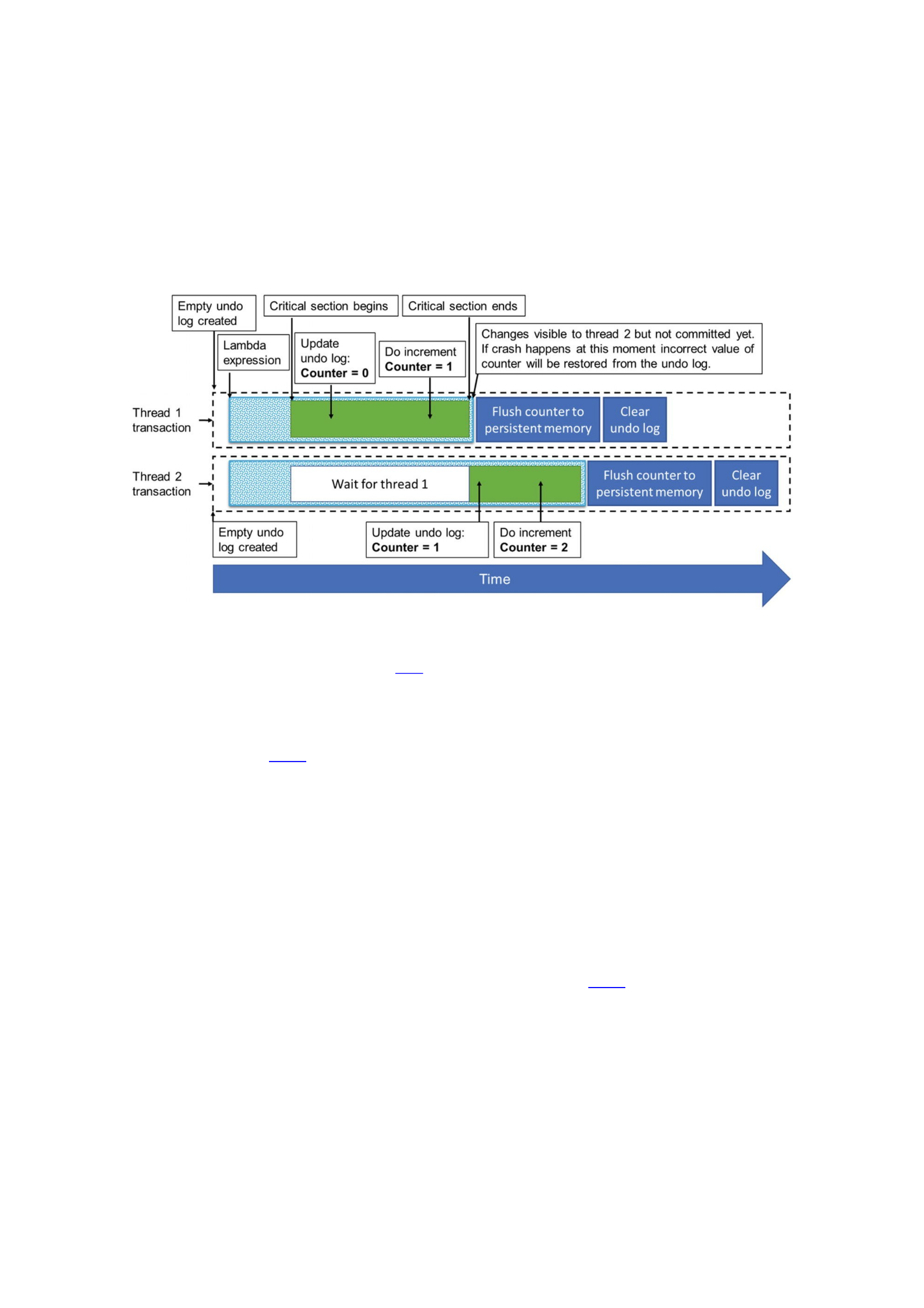
mark the change(s) as committed. Concurrently, the second thread adds the current

value of counter, which is now 1, to its undo log and performs the increment

operation. At that moment, there are two uncommitted transactions. The undo log of

Thread 1 contains counter = 0, and the undo log of Thread 2 contains counter =

1. If Thread 2 commits its transaction while Thread 1 aborts its transaction for some

reason (crash or abort), the incorrect value of counter will be restored from the undo

log of Thread 1.

Figure 14-1Illustrative execution of the Listing 14-2 example

The solution is to hold the mutex until the transaction is fully committed, and the

data has been successfully flushed to persistent memory. Otherwise, changes made by

one transaction become visible to concurrent transactions before it is persisted and

committed. Listing 14-3 demonstrates how to implement the increment() function

correctly.

52 void increment(pop_type &pop) {

53 auto proot = pop.root();

54 pobj::transaction::run(pop, [&] {

55 proot->counter.get_rw() += 1;

56 }, proot->mtx);

57 }

Listing 14-3Correct example for concurrent PMDK transaction

The libpmemobj API allows us to specify locks that should be acquired and held

for the entire duration of the transaction. In the Listing 14-3 example, we pass the

proot->mtx mutex object to the run() method as a third parameter.

Mutexes on Persistent Memory

Our previous examples used pmem::obj::mutex as a type for the mtx member in

our root data structure instead of the regular std::mutex provided by Standard

Template Library. The mtx object is a member of the root object that resides in

persistent memory. The std::mutex type cannot be used on persistent memory

because it may cause persistent deadlock.

A persistent deadlock happens if an application crash occurs while holding a mutex.

When the program starts, if it does not release or reinitialize the mutex at startup,

threads that try to acquire it will wait forever. To avoid such situations, libpmemobj

provides synchronization primitives that reside in persistent memory. The main feature

of synchronization primitives is that they are automatically reinitialized every time the

persistent object store pool is open.

For C++ developers, the libpmemobj-cpp library provides C++11-like

synchronization primitives shown in Table 14-1.

Table 14-1Synchronization primitives provided by libpmemob++ library

Class Description

pmem::obj::mutex This class is an implementation of a persistent memory resident mutex which mimics in

behavior the C++11 std::mutex. This class satisfies all requirements of the Mutex and

StandardLayoutType concepts.

pmem::obj::timed_mutex This class is an implementation of a persistent memory resident timed_mutex which

mimics in behavior the C++11 std::timed_mutex. This class satisfies all requirements of

TimedMutex and StandardLayoutType concepts.

pmem::obj::shared_mutex This class is an implementation of a persistent memory resident shared_mutex which

mimics in behavior the C++17 std::shared_mutex. This class satisfies all requirements of

SharedMutex and StandardLayoutType concepts.

pmem::obj::

condition_variable

This class is an implementation of a persistent memory resident condition variable which

mimics in behavior the C++11 std::condition_variable. This class satisfies all

requirements of StandardLayoutType concept.

For C developers, the libpmemobj library provides pthread-like synchronization

primitives shown in Table 14-2. Persistent memory-aware locking implementations are

based on the standard POSIX Thread Library and provide semantics similar to standard

pthread locks.

Table 14-2Synchronization primitives provided by the libpmemobj library

Structure Description

PMEMmutex The data structure represents a persistent memory resident mutex similar to pthread_mutex_t.

PMEMrwlock The data structure represents a persistent memory resident read-write lock similar to

pthread_rwlock_t.

PMEMcond The data structure represents a persistent memory resident condition variable similar to

pthread_cond_t.

These convenient persistent memory-aware synchronization primitives are

available for C and C++ developers. But what if a developer wants to use a custom

synchronization object that is more appropriate for a particular use case? As we

mentioned earlier, the main feature of persistent memory-aware synchronization

primitives is that they are reinitialized every time we open a persistent memory pool.

The libpmemobj-cpp library provides a more generic mechanism to reinitialize any

user-provided type every time a persistent memory pool is opened.

The libpmemobj-cpp provides the pmem::obj::v<T> class template which

allows creating a volatile field inside a persistent data structure. The mutex object is

semantically a volatile entity, and the state of a mutex should not survive an application

restart. On application restart, a mutex object should be in the unlocked state. The

pmem::obj::v<T> class template is targeted for this purpose. Listing 14-4

demonstrates how to use the pmem::obj::v<T> class template with std::mutex

on persistent memory.

38 namespace pobj = pmem::obj;

40 struct root {

41 pobj::experimental::v<std::mutex> mtx;

42 };

44 using pop_type = pobj::pool<root>;

46 int main(int argc, char *argv[]) {

47 pop_type pop =

48 pop_type::open("/pmemfs/file", "MUTEX");

50 auto proot = pop.root();

52 proot->mtx.get().lock();

54 pop.close();

55 return 0;

56 }

Listing 14-4Example demonstrating usage of std::mutex on persistent memory

Line 41: We are only storing the mtx object inside root object on persistent

memory.

Lines 47-48: We open the persistent memory pool with the layout name of

“MUTEX”.

Line 50: We obtain a pointer to the root data structure within the pool.

Line 52: We acquire the mutex.

Lines 54-56: Close the pool and exit the program.

As you can see, we do not explicitly unlock the mutex within the main() function . If

we run this example several times, the main() function can always lock the mutex on

line 52. This works because the pmem::obj::v<T> class template implicitly calls a

default constructor, which is a wrapped std::mutex object type. The constructor is

called every time we open the persistent memory pool so we never run into a situation

where the lock is already acquired.

If we change the mtx object type on line 41 from

pobj::experimental::v<std::mutex> to std::mutex and try to run the

program again, the example will hang during the second run on line 52 because mtx

object was locked during the first run and we never released it.

Atomic Operations and Persistent Memory

Atomic operations cannot be used inside PMDK transactions for the reason

described in Figure 14-1. Changes made by atomic operations inside a transaction

become visible to other concurrent threads before the transaction is committed. It

forces data inconsistency issues in cases of abnormal program termination or

transaction aborts. Consider lock-free algorithms where concurrency is achieved by

atomically updating the state in memory.

Lock-Free Algorithms and Persistent Memory

It is intuitive to think that lock-free algorithms are naturally fit for persistent

memory. In lock-free algorithms, thread-safety is achieved by atomic transitions

between consistent states, and this is exactly what we need to support data consistency

in persistent memory. But this assumption is not always correct.

To understand the problem with lock-free algorithms, remember that a system with

persistent memory will usually have the virtual memory subsystem divided into two

domains: volatile and persistent (described in Chapter 2). The result of an atomic

operation may only update data in a CPU cache using a cache coherency protocol. There

is no guarantee that the data will be flushed unless an explicit flush operation is called.

CPU caches are only included within the persistence domain on platforms with eADR

support. This is not mandatory for persistent memory. ADR is the minimal platform

requirement for persistent memory, and in that case, CPU caches are not flushed in a

power failure.

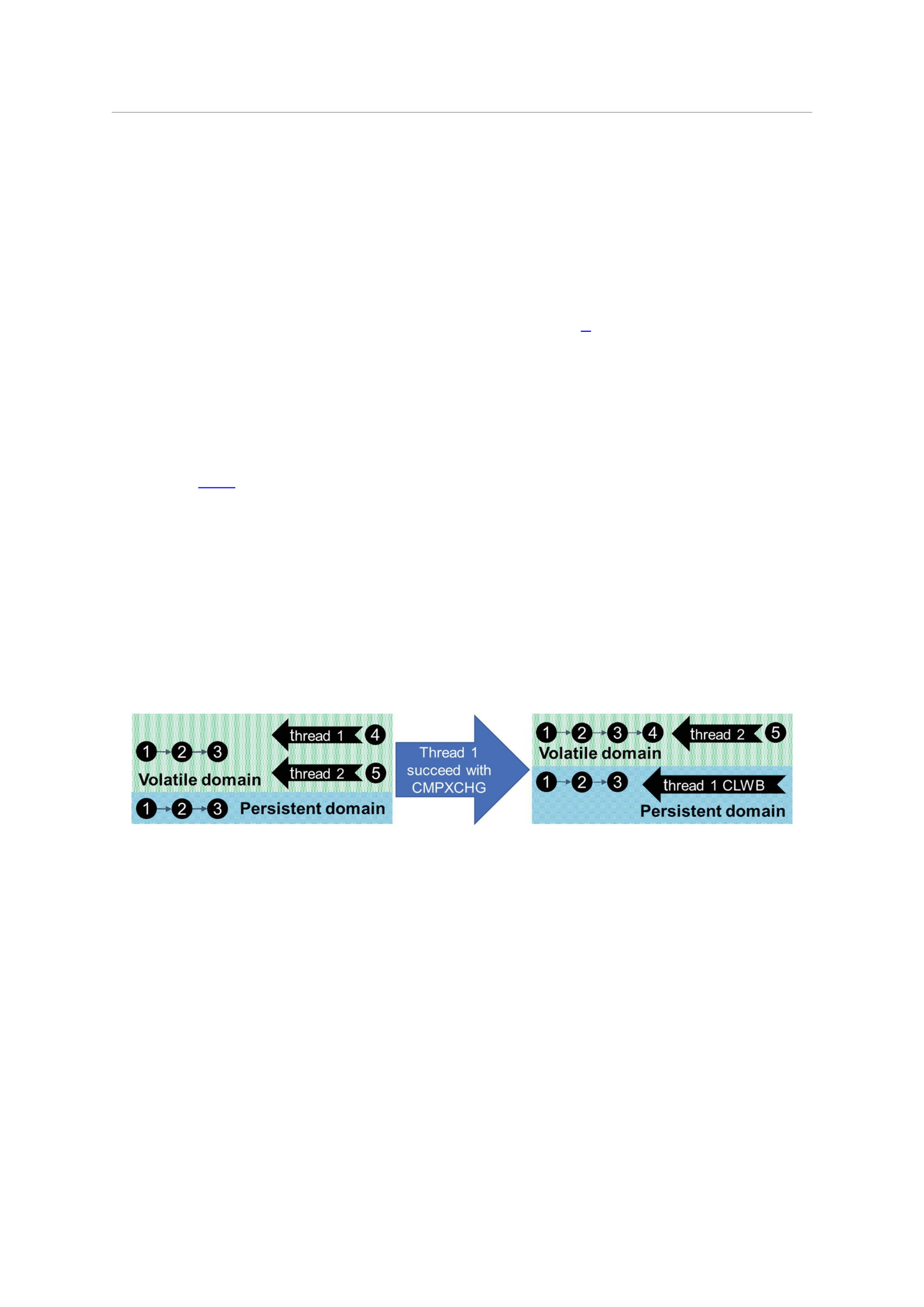
Figure 14-2 assumes a system with ADR support. The example shows concurrent

lock-free insert operations to a singly linked list located in persistent memory. Two

threads are trying to insert new nodes to the tail of a linked list using a compare-and-

exchange (CMPXCHG instruction) operation followed by a cache flush operation (CLWB

instruction) . Assume Thread 1 succeeds with its compare-and-exchange, so the change

appears in a volatile domain and becomes visible to the second thread. At this moment,

Thread 1 may be preempted (changes not flushed to a persistent domain), while Thread

2 inserts Node 5 after Node 4 and flushes it to a persistent domain. A possibility for data

inconsistency exists because Thread 2 performed an update based on the data that is

not yet persisted by Thread 1.

Figure 14-2Example of a concurrent lock-free insert operation to a singly linked list located in persistent memory

Concurrent Data Structures for Persistent Memory

This section describes two concurrent data structures available in the

libpmemobj-cpp library: pmem::obj::concurrent_map and

pmem::obj::concurrent_hash_map. Both are associative data structures

composed of a collection of key and value pairs, such that each possible key appears at

most once in the collection. The main difference between them is that the concurrent

hash map is unordered, while the concurrent map is ordered by keys.

We define concurrent in this context to be the method of organizing data structures

for access by multiple threads. Such data structures are intended for use in a parallel

computing environment when multiple threads can concurrently call methods of a data

structure without additional synchronization required.

C++ Standard Template Library (STL) data structures can be wrapped in a coarse-

grained mutex to make them safe for concurrent access by letting only one thread

operate on the container at a time. However, that approach eliminates concurrency and

thereby restricts parallel speedup if implemented in performance-critical code.

Designing concurrent data structures is a challenging task. The difficulty increases

significantly when we need to develop concurrent data structures for persistent

memory and make them fault tolerant.

The pmem::obj::concurrent_map and

pmem::obj::concurrent_hash_map structures were inspired by the Intel

Threading Building Blocks (Intel TBB),1 which provides implementations of these

concurrent data structures designed for volatile memory. You can read the Pro TBB: C++

Parallel Programming with Threading Building Blocks book2 to get more information

and learn how to use these concurrent data structures in your application. The free

electronic copy is available from Apress at

https://www.apress.com/gp/book/9781484243978.

There are three main methods in our concurrent associative data structures: find,

insert, and erase/delete. We describe each data structure with a focus on these

three methods.

Concurrent Ordered Map

The implementation of the concurrent ordered map for persistent memory

(pmem::obj::concurrent_map) is based on a concurrent skip list data structure.

Intel TBB supplies tbb::concurrent_map, which is designed for volatile memory

that we use as a baseline for a port to persistent memory. The concurrent skip list data

structure can be implemented as a lock-free algorithm. But Intel chose a provably

correct scalable concurrent skip list3 implementation with fine-grain locking

distinguished by a combination of simplicity and scalability. Figure 14-3 demonstrates

the basic idea of the skip list data structure. It is a multilayered linked list-like data

structure where the bottom layer is an ordered linked list. Each higher layer acts as an

“express lane” for the following lists and allows it to skip elements during lookup

operations. An element in layer i appears in layer i+1 with some fixed probability p (in

our implementation p = 1/2). That is, the frequency of nodes of a particular height

decreases exponentially with the height. Such properties allow it to achieve O(log n)

average time complexity for lookup, insert, and delete operations. O(log n) means the

running time grows at most proportional to “log n”. You can learn more about Big O

notation on Wikipedia at https://en.wikipedia.org/wiki/Big_O_notation

For the implementation of pmem::obj::concurrent_map, the find and

insert operations are thread-safe and can be called concurrently with other find and

insert operations without requiring additional synchronizations.

Find Operation

Because the find operation is non-modifying, it does not have to deal with data

consistency issues. The lookup operation for the target element always begins from

the topmost layer. The algorithm proceeds horizontally until the next element is greater

or equal to the target. Then it drops down vertically to the next lower list if it cannot

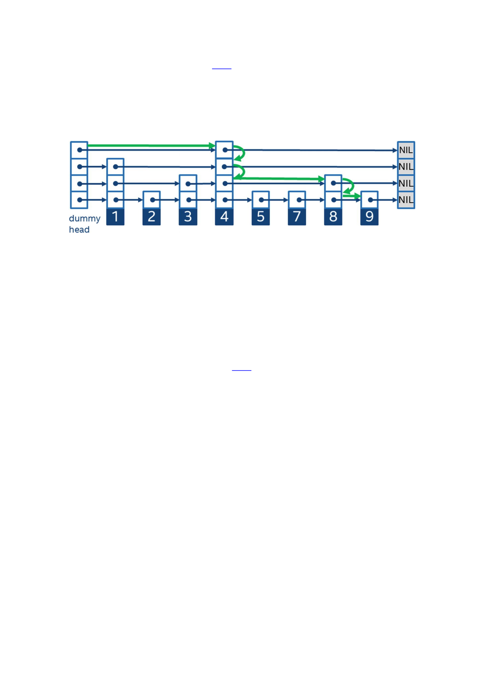
proceed on the current level. Figure 14-3 illustrates how the find operation works for

the element with key=9. The search starts from the highest level and immediately goes

from dummy head node to the node with key=4, skipping nodes with keys 1, 2, 3. On the

node with key=4, the search is dropped two layers down and goes to the node with

key=8. Then it drops one more layer down and proceeds to the desired node with

key=9.

Figure 14-3Finding key=9 in the skip list data structure

The find operation is wait-free. That is, every find operation is bound only by the

number of steps the algorithm takes. And a thread is guaranteed to complete the

operation regardless of the activity of other threads. The implementation of

pmem::obj::concurrent_map uses atomic load-with-acquire memory semantics

when reading pointers to the next node.

Insert Operation

The insert operation , shown in Figure 14-4, employs fine-grained locking schema for

thread-safety and consists of the following basic steps to insert a new node with key=7

into the list:

Allocate the new node with randomly generated height.

2. Find a position to insert the new node. We must find the predecessor and successor

nodes on each level.

3. Acquire locks for each predecessor node and check that the successor nodes have not

been changed. If successor nodes have changed, the algorithm returns to step 2.

4. Insert the new node to all layers starting from the bottom one. Since the find

operation is lock-free, we must update pointers on each level atomically using store-

with-release memory semantics.

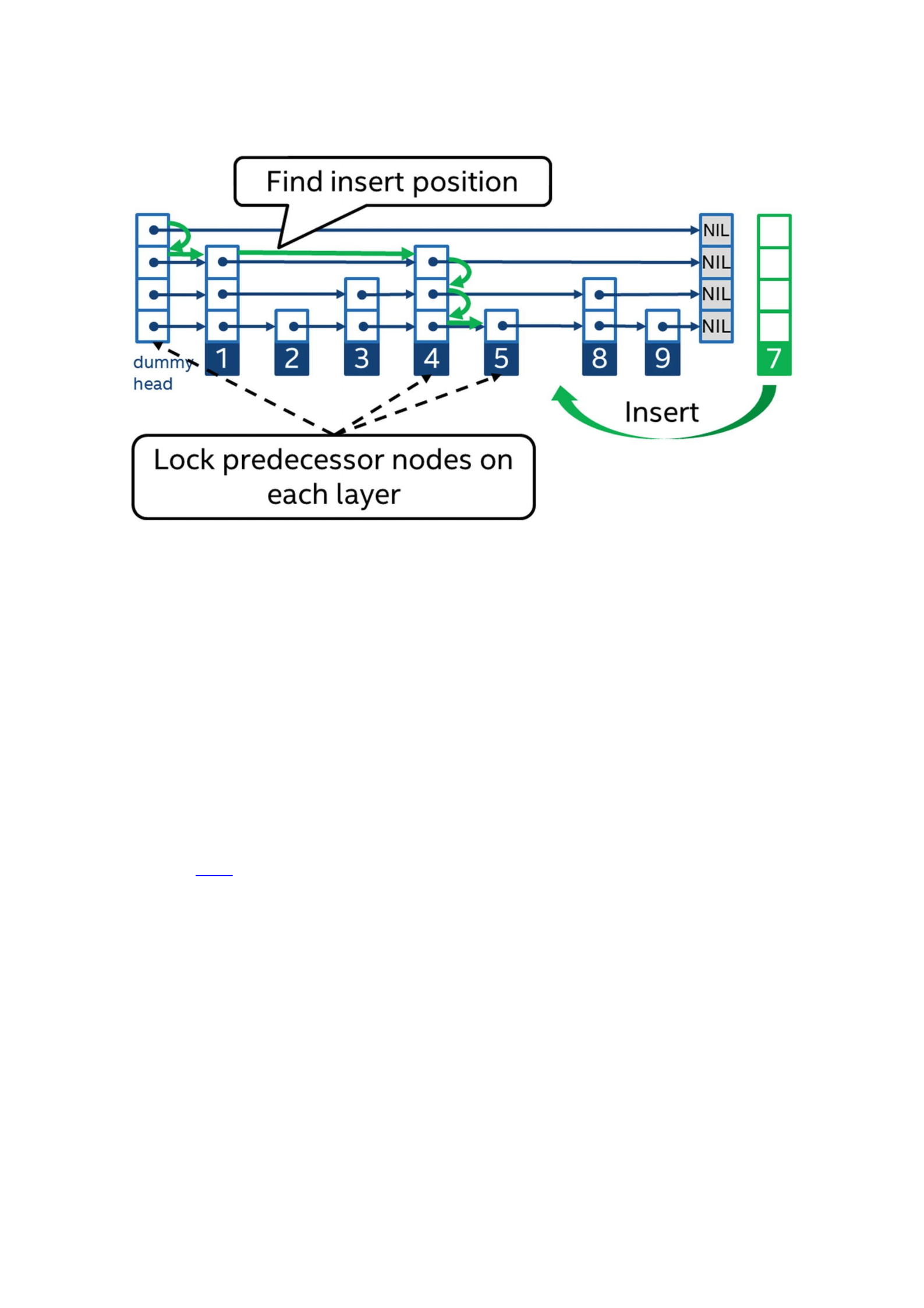
Figure 14-4Inserting a new node with key=7 into the concurrent skip list

The algorithm described earlier is thread-safe, but it is not enough to be fault

tolerant on persistent memory. There is a possible persistent memory leak if a program

unexpectedly terminates between the first and fourth steps of our algorithm.

The implementation of pmem::obj::concurrent_map does not use transactions

to support data consistency because transactions do not support isolation and by not

using transactions, it can achieve better performance. For this linked list data structure,

data consistency is maintained because a newly allocated node is always reachable (to

avoid persistent memory leak) and the linked list data structure is always valid. To

support these two properties, persistent thread-local storage is used, which is a

member of the concurrent skip list data structure. Persistent thread-local storage

guarantees that each thread has its own location in persistent memory to assign the

result of persistent memory allocation for the new node.

Figure 14-5 illustrates the approach of this fault-tolerant insert algorithm. When a

thread allocates a new node, the pointer to that node is kept in persistent thread-local

storage, and the node is reachable through this persistent thread-local storage. Then the

algorithm inserts the new node to the skip list by linking it to all layers using the thread-

safe algorithm described earlier. Finally, the pointer in the persistent thread-local

storage is removed because the new node is reachable now via skip list itself. In case of

failure, a special function traverses all nonzero pointers in persistent thread-local

storage and completes the insert operation .

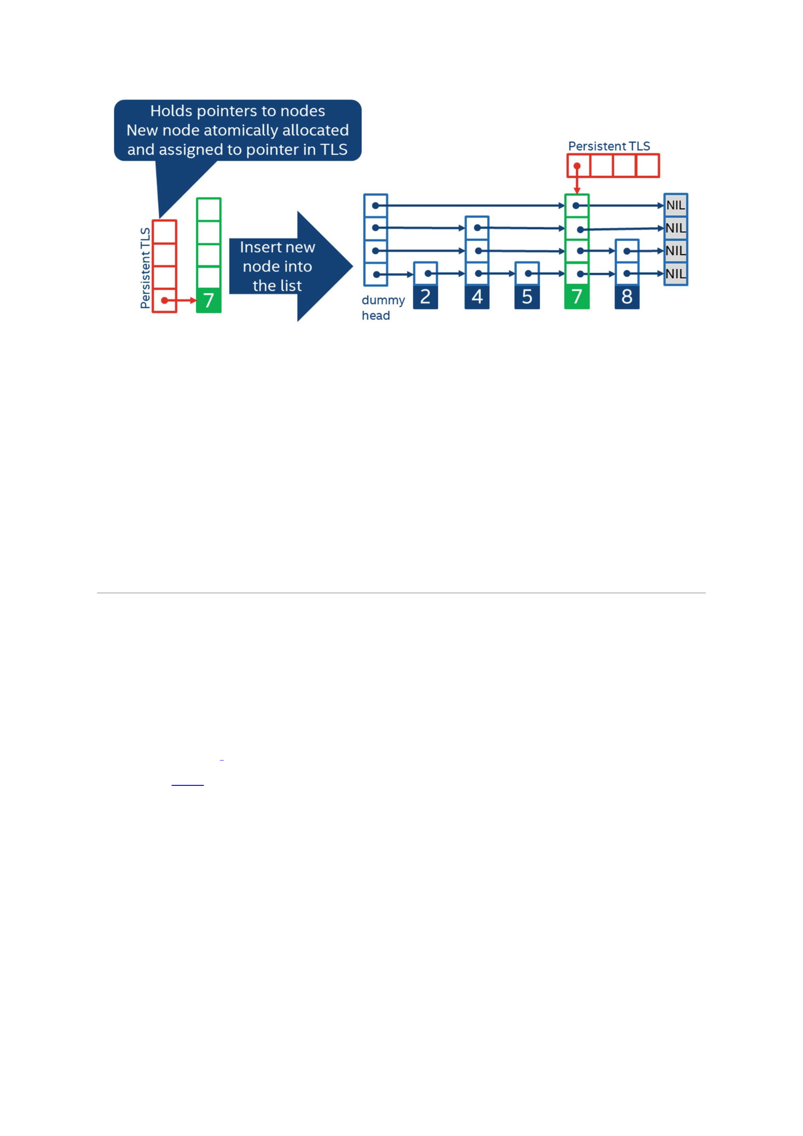
Figure 14-5Fault-tolerant insert operation using persistent thread-local storage

Erase Operation

The implementation of the erase operation for pmem::obj::concurrent_map

is not thread-safe. This method cannot be called concurrently with other methods of the

concurrent ordered map because this is a memory reclamation problem that is hard to

solve in C++ without a garbage collector. There is a way to logically extract a node from

a skip list in a thread-safe manner, but it is not trivial to detect when it is safe to delete

the removed node because other threads may still have access to the node. There are

possible solutions, such as hazard pointers, but these can impact the performance of the

find and insert operations.

Concurrent Hash Map

The concurrent hash map designed for persistent memory is based on

tbb::concurrent_hash_map that exists in the Intel TBB. The implementation is

based on a concurrent hash table algorithm where elements assigned to buckets based

on a hash code are calculated from a key. In addition to concurrent find, insert,

and erase operations, the algorithm employs concurrent resizing and on-demand per-

bucket rehashing.4

Figure 14-6 illustrates the basic idea of the concurrent hash table. The hash table

consists of an array of buckets, and each bucket consists of a list of nodes and a read-

write lock to control concurrent access by multiple threads.

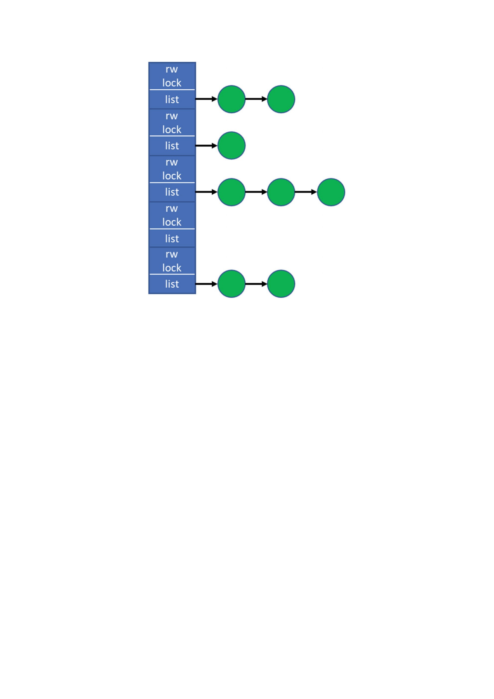
Figure 14-6The concurrent hash map data structure

Find Operation

The find operation is a read-only event that does not change the hash map state.

Therefore, data consistency is maintained while performing a find request. The find

operation works by first calculating the hash value for a target key and acquires read

lock for the corresponding bucket. The read lock guarantees that there is no concurrent

modifications to the bucket while we are reading it. Inside the bucket, the find

operation performs a linear search through the list of nodes.

Insert Operation

The insert method of the concurrent hash map uses the same technique to support

data consistency as the concurrent skip list data structure. The operation consists of the

following steps:

Allocate the new node, and assign a pointer to the new node to persistent thread-

local storage.

2. Calculate the hash value of the new node, and find the corresponding bucket.

3. Acquire the write lock to the bucket.

4. Insert the new node to the bucket by linking it to the list of nodes. Because only one

pointer has to be updated, a transaction is not needed. Because only one pointer is

updated, a transaction is not required.

Erase Operation

Although the erase operation is similar to an insert (the opposite action), its

implementation is even simpler than the insert. The erase implementation acquires

the write lock for the required bucket and, using a transaction, removes the

corresponding node from the list of nodes within that bucket.

Performance Analysis Concepts

Most concepts for performance analysis of persistent memory are similar to those

already established for performance analysis of shared memory programs or storage

bottlenecks. This section outlines several important performance considerations you

should understand to profile and optimize persistent memory performance and defines

the terms and situations we use in this chapter.

Compute-Bound vs. Memory-Bound

Performance optimization largely involves identifying the current performance

bottleneck and improving it. The performance of compute-bound workloads is generally

limited by the number of instructions the CPU can process per cycle. For example, an

application doing a large number of calculations on very compact data without many

dependencies is usually compute-bound . This type of workload would run faster if the

CPU were faster. Compute-bound applications usually have high CPU utilization, close to

100%.

In contrast, the performance of memory-bound workloads is generally limited by the

memory subsystem and the long latencies of fetching data from caches and system

memory. An example is an application that randomly accesses data from data structures

in DRAM. In this case, adding more compute resources would not improve such an

application. Adding persistent memory to improve performance is usually an option for

memory-bound workloads as opposed to compute-bound workloads. Memory-bound

workloads usually have lower CPU utilization than compute-bound workloads, exhibit

CPU stalls due to memory transfers, and have high memory bandwidth.

Memory Latency vs. Memory Capacity

This concept is essential when discussing persistent memory. For this discussion, we

assume that DRAM access latencies are lower than persistent memory and that the

persistent memory capacity within the system is larger than DRAM. Workloads bound

by memory capacity can benefit from adding persistent memory in a volatile mode,

while workloads that are bound by memory latency are less likely to benefit.

Read vs. Write Performance

While each persistent memory technology is unique, it is important to understand

that there is usually a difference in the performance of reads (loads) vs. writes (stores).

Different media types exhibit varying degrees of asymmetric read-write performance

characteristics, where reads are generally much faster than writes. Therefore,

understanding the mix of loads and stores in an application workload is important for

understanding and optimizing performance.

Memory Access Patterns

A memory access pattern is the pattern with which a system or application reads

and writes to or from the memory. Memory hardware usually relies on temporal locality

(accessing recently used data) and spatial locality (accessing contiguous memory

addresses) for best performance. This is often achieved through some structure of fast

internal caches and intelligent prefetchers. The access pattern and level of locality can

drastically affect cache performance and can also have implications on parallelism and

distributions of workloads within shared memory systems. Cache coherency can also

affect multiprocessor performance, which means that certain memory access patterns

place a ceiling on parallelism. Many well-defined memory access patterns exist,

including but not limited to sequential, strided, linear, and random.

It is much easier to measure, control, and optimize memory accesses on systems that

run only one application. In the cloud and virtualized environments, applications within

the guests can be running any type of application and workload, including web servers,

databases, or an application server. This makes it much harder to ensure memory

accesses are fully optimized for the hardware as the access patterns are essentially

random.

I/O Storage Bound Workloads

A program is I/O bound if it would go faster if the I/O subsystem were faster. We are

primarily interested in the block-based disk I/O subsystem here, but it could also

include other subsystems such as the network. An I/O bound state is undesirable

because it means that the CPU must stall its operation while waiting for data to be

loaded or unloaded from main memory or storage. Depending on where the data is and

the latency of the storage device, this can invoke a voluntary context switching of the

current application thread with another. A voluntary context switch occurs when a

thread blocks because it requires a resource that is not immediately available or takes a

long time to respond. With faster computation speed being the primary goal of each

successive computer generation, there is a strong imperative to avoid I/O bound states.

Eliminating them can often yield a more economic improvement in performance than

upgrading the CPU or memory.

Determining the Suitability of Workloads for Persistent

Memory

Persistent memory technologies may not solve every workload performance

problem. You should understand the workload and platform on which it is currently

running when considering persistent memory. As a simple example, consider a

compute-intensive workload that relies heavily on floating-point arithmetic. The

performance of this application is likely limited by the floating-point unit in the CPU and

not any part of the memory subsystem. In that case, adding persistent memory to the

platform will likely have little impact on this application’s performance. Now consider

an application that requires extensive reading and writing from disk. It is likely that the

disk accesses are the bottleneck for this application and adding a faster storage solution,

like persistent memory, could improve performance.

These are trivial examples, and applications will have widely different behaviors

along this spectrum. Understanding what behaviors to look for and how to measure

them is an important step to using persistent memory. This section presents the

important characteristics to identify and determine if an application is a good fit for

persistent memory. We look at applications that require in-memory persistence,

applications that can use persistent memory in a volatile manner, and applications that

can use both.

Volatile Use Cases

Chapter 10 described several libraries and use cases where applications can take

advantage of the performance and capacity of persistent memory to store non-volatile

data. For volatile use cases, persistent memory will act as an additional memory tier for

the platform. It may be transparent to the application, such as using Memory Mode

supported by Intel Optane DC persistent memory, or applications can make code

changes to perform volatile memory allocations using libraries such as libmemkind. In

both cases, memory-capacity bound workloads will benefit from adding persistent

memory to the platform. Application performance can dramatically improve if its

working dataset can fit into memory and avoid paging to disk.

Identifying Workloads That Are Memory-Capacity Bound

To determine if a workload is memory-capacity bound, you must determine the

“memory footprint” of the application. The memory footprint is the high watermark of

memory concurrently allocated during the application’s life cycle. Since physical

memory is a finite resource, you should consider the fact that the operating system and

other processes also consume memory. If the footprint of the operating system and all

memory consumers on the system are approaching or exceeding the available DRAM

capacity on the platform, you can assume that the application would benefit from

additional memory because it cannot fit all its data in DRAM. Many tools and techniques

can be used to determine memory footprint. VTune Profiler includes two different ways

to find this information: Memory Consumption analysis or Platform Profiler analysis.

VTune Profiler is a free download for Linux and Windows, available from

https://software.intel.com/en-us/vtune.

The Memory Consumption analysis within VTune Profiler tracks all memory

allocations made by the application. Figure 15-1 shows a VTune Profiler bottom-up

report representing memory consumption of the profiled application over time. The

highest value on the y-axis in the Memory Consumption timeline indicates the

application footprint is approximately 1GiB.

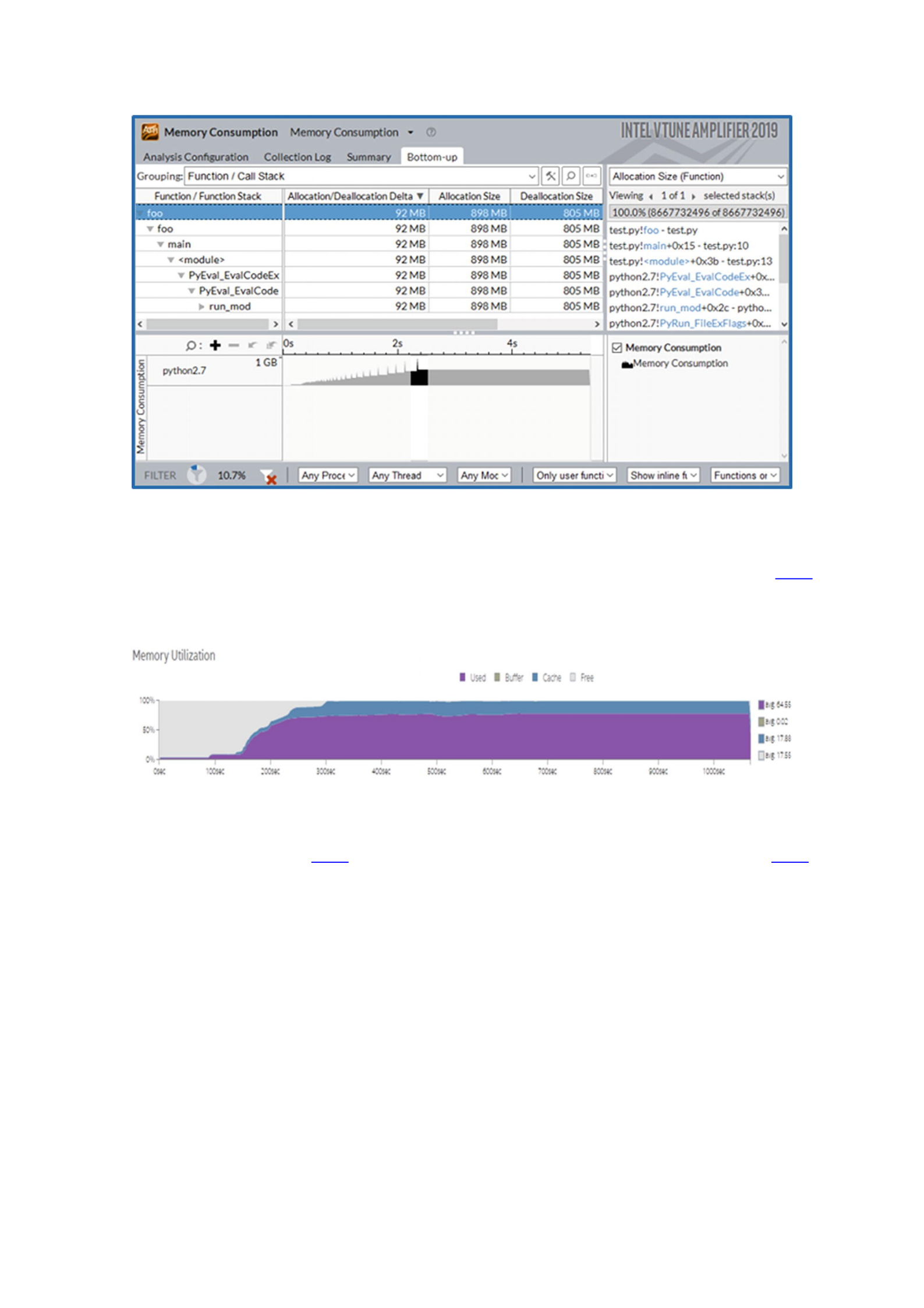
Figure 15-1The VTune Profiler bottom-up analysis showing memory consumption with time and the associated

allocating call stacks

The Memory Utilization graph in the Platform Profiler analysis shown in Figure 15-2

measures the memory footprint using operating system statistics and produces a

timeline graph as a percentage of the total available memory.

Figure 15-2The VTune Platform Profiler Memory Utilization graph as a percentage of total system memory

The results in Figure 15-2 were taken from a different application than Figure 15-1.

This graph shows very high memory consumption, which implies this workload would

be a good candidate for adding more memory to the system. If your persistent memory

hardware has variable modes, like the Memory and App Direct modes on Intel Optane

DC persistent memory, you will need some more information to determine which mode

to use first. The next important information is the hot working set size.

Identifying the Hot Working Set Size of a Workload

Persistent memory usually has different characteristics than DRAM; therefore, you

should make intelligent decisions about where data will reside. We will assume that

accessing data from persistent memory has higher latency than DRAM. Given the choice

between accessing data in DRAM and persistent memory, we would always choose

DRAM for performance. However, the premise of adding persistent memory in a volatile

configuration assumes there is not enough DRAM to fit all the data. You need to

understand how your workload accesses data to make choices about persistent memory

configuration.

The working set size (WSS) is how much memory an application needs to keep

working. For example, if an application has 50GiB of main memory allocated and page

mapped, but it is only accessing 20MiB each second to perform its job, we can say that

the working set size is 50GiB and the “hot” data is 20MiB. It is useful to know this for

capacity planning and scalability analysis. The “hot working set” is the set of objects

accessed frequently by an application, and the “hot working set size” is the total size of

those objects allocated at any given time.

Determining the size of the working set and hot working set is not as

straightforward as determining memory footprint. Most applications will have a wide

range of objects with varying degrees of “hotness,” and there will not be a clear line

delineating which objects are hot and which are not. You must interpret this

information and determine the hot working set size.

VTune Profiler has a Memory Access analysis feature that can help determine the

hot and working set sizes of an application (select the “Analyze dynamic memory

objects” option before data collection begins). Once enough data has been collected,

VTune Profiler will process the data and produce a report. In the bottom-up view within

the GUI, a grid lists each memory object that was allocated by the application.

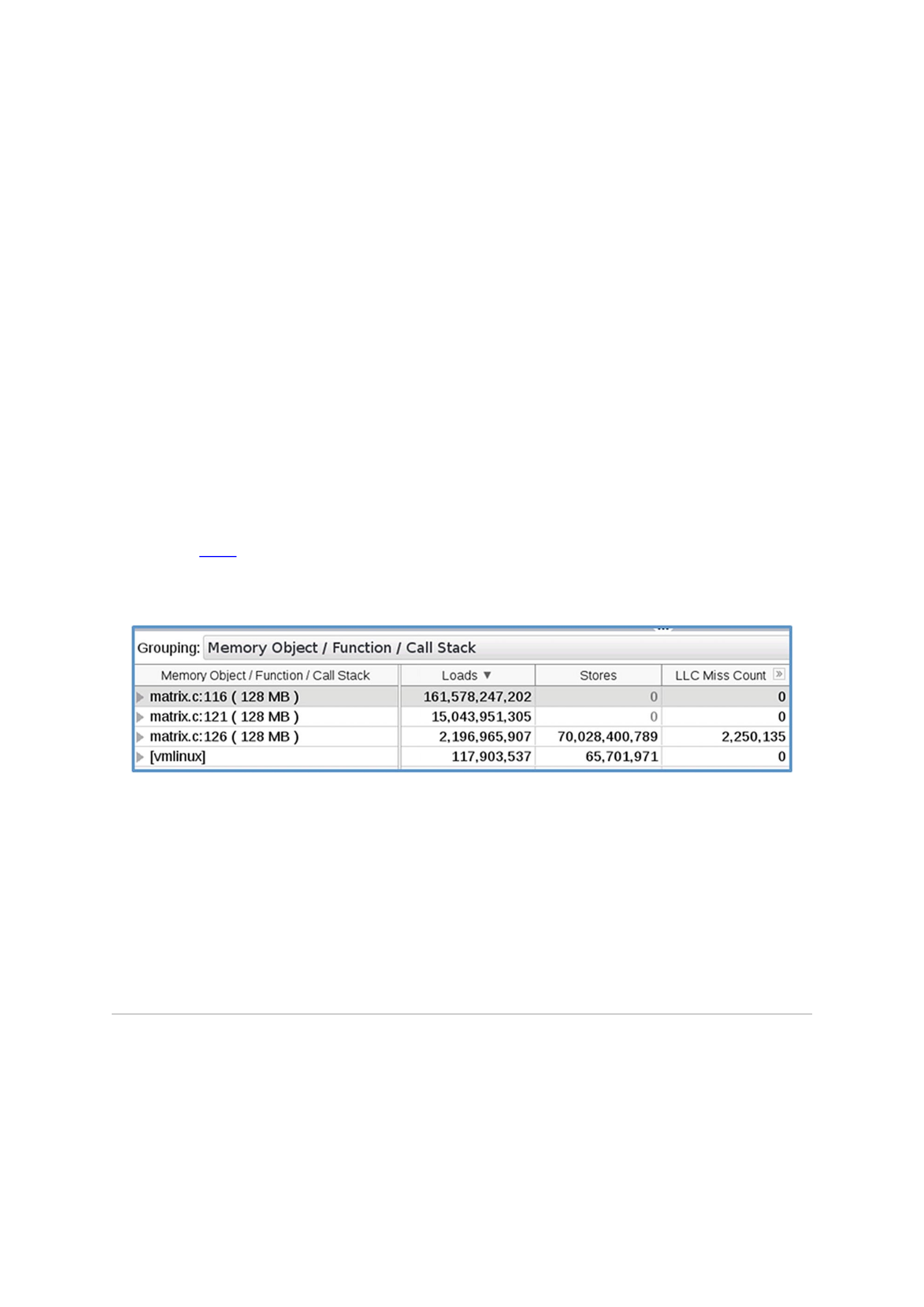
Figure 15-3 shows the results of a Memory Access analysis of an application. It

shows the memory size in parenthesis and the number of loads and stores that accessed

it. The report does not include an indication of what was concurrently allocated.

Figure 15-3Objects accessed by the application during a Memory Access analysis data collection

The report identifies the objects with the most accesses (loads and stores). The sum

of the sizes of these objects is the working set size – the values are in parentheses. You

decide where to draw the line for what is and is not part of the hot working set.

Depending on the workload, there may not be an easy way to determine the hot

working set size, other than developer knowledge of the application. Having a rough

estimate is important for deciding whether to start with Memory Mode or App Direct

mode.

Use Cases Requiring Persistence

Use cases that take advantage of persistent memory for persistence, as opposed to the

volatile use cases previously described, are generally replacing slower storage devices

with persistent memory. Determining the suitability of a workload for this use case is

straightforward. If application performance is limited by storage accesses (disks, SSDs,

etc.), then using a faster storage solution like persistent memory could help. There are

several ways to identify storage bottlenecks in an application. Open source tools like

dstat or iostat give a high-level overview of disk activity, and tools such as VTune

Profiler provide a more detailed analysis.

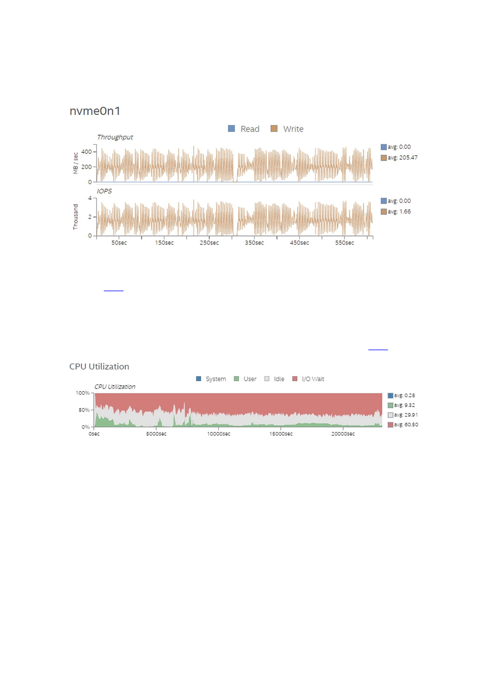
Figure 15-4Disk throughput and IOPS graphs from VTune Profiler’s Platform Profiler

Figure 15-4 shows throughput and IOPS numbers of an NVMe drive collected using

Platform Profiler. This example uses a non-volatile disk for extensive storage, as

indicated by the throughput and IOPS graphs. Applications like this may benefit from

faster storage like persistent memory. Another important metric to identify storage

bottlenecks is I/O Wait time. The Platform Profiler analysis can also provide this metric

and display how it is affecting CPU Utilization over time, as seen in Figure 15-5.

Figure 15-5I/O Wait time from VTune Profiler’s Platform Profiler

Performance Analysis of Workloads Using Persistent

Memory

Optimizing a workload on a system with persistent memory follows the principles

similar to those of optimizing a workload performance on a DRAM-only system. The

additional factors to keep in mind are:

The writes to persistent memory may impact performance more than the

reads.

Applications can allocate objects on DRAM or persistent memory. If done

indiscriminately, this can negatively impact performance.

In Memory Mode (specific to Intel Optane DC persistent memory), users

have the option of varying the near-memory cache size (DRAM size) to

improve workload performance.

Keeping these additional factors in mind, the approach to workload performance

optimization will follow the same process of characterizing the workload, choosing the

correct memory configuration, and optimizing the code for maximum performance.

Characterizing the Workload

The performance of a workload on a persistent memory system depends on a

combination of the workload characteristics and the underlying hardware. The key

metrics to understand the workload characteristics are:

Persistent memory bandwidth

Persistent memory read/write ratio

Paging to and from traditional storage

Working set size and footprint of the workload

Nonuniform Memory Architecture (NUMA) characteristics

Near-memory cache behavior in Memory Mode (specific to Intel Optane DC

persistent memory)

Memory Bandwidth and Latency

Persistent memory, like DRAM, has limited bandwidth. When it becomes saturated,

it can quickly bottleneck application performance. Bandwidth limits will vary

depending on the platform. You can calculate the peak bandwidth of your platform

using hardware specifications or a memory benchmarking application.

The Intel Memory Latency Checker (Intel MLC) is a free tool for Linux and Windows

available from https://software.intel.com/en-us/articles/intelr-

memory-latency-checker. Intel MLC can be used to measure bandwidth and

latency of DRAM and persistent memory using a variety of tests:

Measure idle memory latencies between each CPU socket

Measure peak memory bandwidth requests with varying ratios of reads and

writes

Measure latencies at different bandwidth points

Measure latencies for requests addressed to a specific memory controller

from a specific core

Measure cache latencies

Measure b/w from a subset of the cores/sockets

Measure b/w for different read/write ratios

Measure latencies for random and sequential address patterns

Measure latencies for different stride sizes

Measure cache-to-cache data transfer latencies

VTune Profiler has a built-in kernel to measure peak bandwidth on a system. Once

you know the peak bandwidth of the platform, you can then measure the persistent

memory bandwidth of your workload. This will reveal whether persistent memory

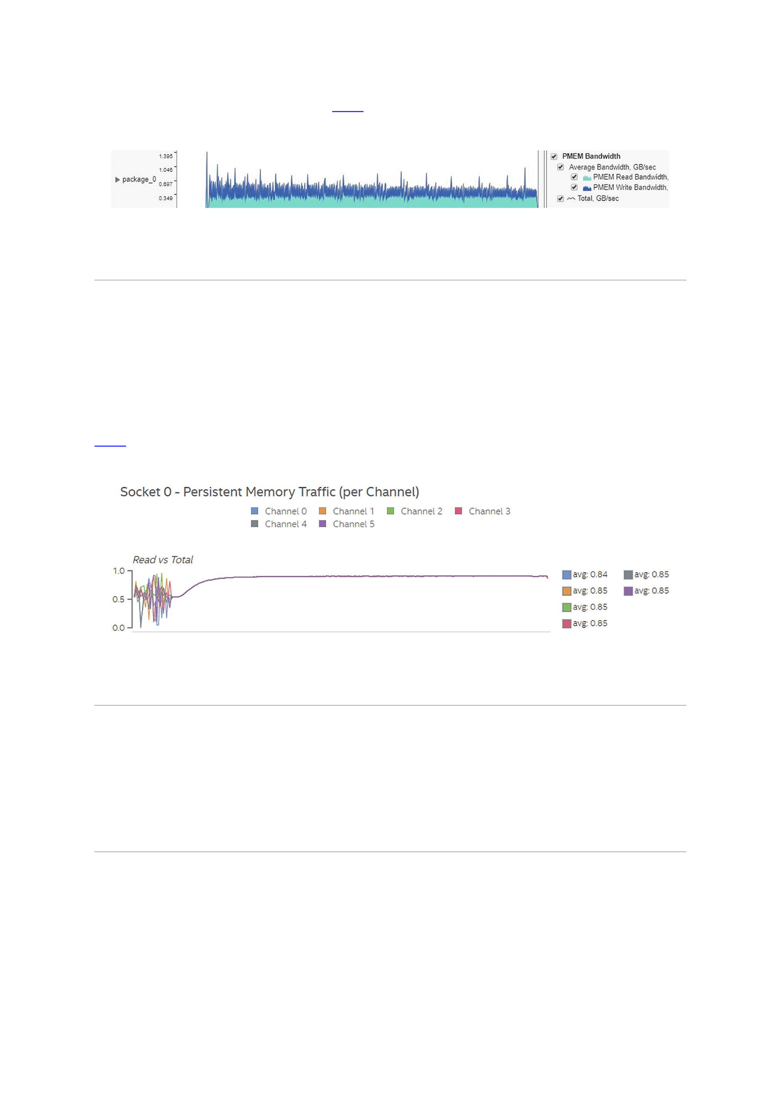
bandwidth is a bottleneck. Figure 15-6 shows an example of persistent memory read

and write bandwidth of an application.

Figure 15-6Results from VTune Profiler persistent memory bandwidth measurements

Persistent Memory Read-Write Ratio

As described in “Performance Analysis Concepts,” the ratio of read and write traffic to

the persistent memory plays a major role in the overall performance of a workload. If

the ratio of persistent memory write bandwidth to read bandwidth is high, there is a

good chance the persistent memory write latency is impacting performance. Using the

Platform Profiler feature in VTune Profiler is one way to collect this information. Figure

15-7 shows the ratio of read traffic vs. all traffic to persistent memory. This number

should be close to 1.0 for best performance.

Figure 15-7Read traffic ratio from VTune Profiler’s Platform Profiler analysis

Working Set Size and Memory Footprint

As described in “Determining the Suitability of Workloads for Persistent Memory,”

the working set size and memory footprint of the application are important

characteristics to understand once a workload is running on a system with persistent

memory. Metrics can be collected using the tools and processes previously described.

Non-Uniform Memory Architecture (NUMA) Behavior

Multi-socket platforms typically have persistent memory attached to each socket.

Accesses to persistent memory from a thread on one socket to another will incur longer

latencies. These “remote” accesses are some of the NUMA behaviors that can impact

performance. Multiple metrics can be collected to determine how much NUMA activity

is occurring in a workload. On Intel platforms, data moves between sockets through the

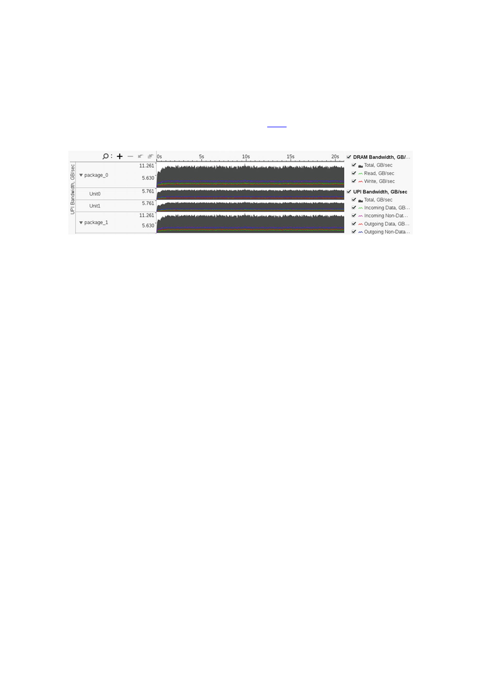
socket interconnect called the QuickPath Interconnect (QPI) or Ultra Path Interconnect

(UPI) . High interconnect bandwidth may indicate NUMA-related performance issues. In

addition to interconnect bandwidth, some hardware provides counters to track local

and remote accesses to persistent memory.

Understanding the NUMA behavior of your workload is another important step in

understanding performance optimization. Figure 15-8 shows UPI bandwidth collected

with VTune Profiler.

Figure 15-8UPI traffic ratio from VTune Profiler

The Platform Profiler feature in VTune Profiler can collect metrics specific to

persistent memory.

Tuning the Hardware

The memory configuration of a system is a significant factor in determining the

system’s performance. The workload performance depends on a combination of

workload characteristics and the memory configuration. There is no single

configuration that provides the best value for all workloads. These factors make it

important to tune the hardware with respect to workload characteristics and get the

maximum value out of the system.

Addressable Memory Capacity

The combined capacity of DRAM and persistent memory determines the total

addressable memory available on the system. You should tune the size of persistent

memory to accommodate the workload’s footprint.

The capacity of DRAM available on the system should be large enough to

accommodate the workload’s hot working set size. A large amount of volatile traffic

going to persistent memory while DRAM is fully utilized is a good indicator that the

workload can benefit from additional DRAM size.

Bandwidth Requirements

The maximum available persistent memory bandwidth depends on the number of

channels populated with a persistent memory module. A fully populated system works

well for a workload with a high bandwidth requirement. Partially populated systems

can be used for workloads that are not as memory latency sensitive. Refer to the server

documentation for population guidelines.

BIOS Options

With the introduction of persistent memory into server platforms, many features and

options have been added to the BIOS that provide additional tuning capabilities. The

options and features available within the BIOS vary for each server vendor and

persistent memory product. Refer to the server BIOS documentation for all the options

available; most share common options, including:

Ability to change power levels to balance power consumption and

performance. More power delivered to persistent memory can increase

performance

Enable or disable persistent memory–specific features

Tune latency or bandwidth characteristics of persistent memory

Optimizing the Software for Persistent Memory

There are many ways to optimize applications to use persistent memory efficiently

and effectively. Each application will benefit in different ways and will need to have

code modified accordingly. This section describes some of the optimization methods.

Guided Data Placement

Guided data placement is the most common avenue for optimizing volatile

workloads on a persistent memory system. Application developers can choose to

allocate a data structure or object in DRAM or persistent memory. It is important to

choose accurately because allocating incorrectly could impact application performance.

This allocation is usually handled via specific APIs, for example, the allocation APIs

available in the Persistent Memory Development Kit (PMDK) and memkind library.

Depending on your familiarity with the code and how it works with production

workloads, knowing which data structures and objects to store in the different

memory/storage tiers may be simple. Should those data structures and objects be

volatile or persisted? To help with searching for potential candidates, tools such as

VTune Profiler can identify objects with the most last-level cache (LLC) misses. The

intent is to identify what data structures and objects the application uses most

frequently and ensure they are placed in the fastest media appropriate to their access

patterns. For example, an object that is written once but read many times is best placed

in DRAM. An object that is updated frequently that needs to be persisted should

probably be moved to persistent memory rather than traditional storage devices.

You must also be mindful of memory-capacity constraints. Tools such as VTune

Profiler can help determine approximately how many hot objects will fit into the

available DRAM. For the remaining objects that have fewer LLC misses or that are too

large to allocate from DRAM, you can put them in persistent memory. These steps will

ensure that your most accessed objects have the fastest path to the CPU (allocated in

DRAM), while the infrequently accessed objects will take advantage of the additional

persistent memory (as opposed to sitting out on a much slower storage devices).

Another consideration for optimizations is the load/store ratio for object accesses. If

your persistent memory hardware characteristics are such that load/read operations

are much faster than stores/writes, this should be taken into account. Objects with a

high load/store ratio should benefit from living in persistent memory.

There is no hard rule for what constitutes a frequent vs. infrequently accessed

object. Although behaviors are application dependent, these guidelines give a starting

point for choosing how to allocate objects in persistent memory. After completing this

process, start profiling and tuning the application to further improve the performance

with persistent memory.

Memory Access Optimization

The common techniques for optimizing cache performance on DRAM-only platforms

also apply to persistent memory platforms. Concepts like cache-miss penalties and

spatial/temporal data locality are important for performance. Many tools can collect

performance data for caches and memory. VTune Profiler has predefined metrics for

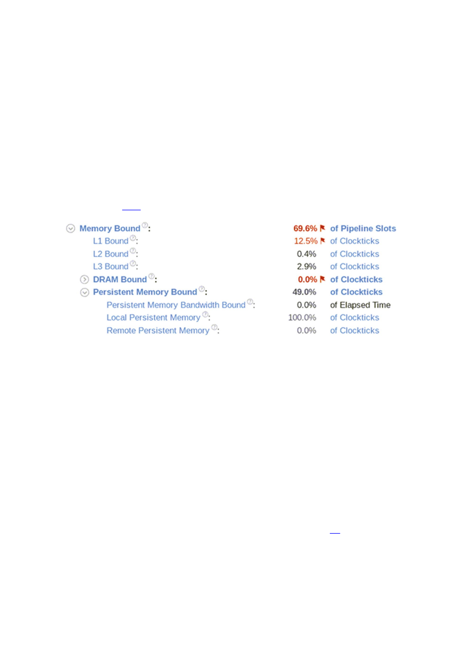
each level of the memory hierarchy, including Intel Optane DC persistent memory

shown in Figure 15-9.

Figure 15-9VTune Profiler memory analysis of a workload showing a breakdown of CPU cache, DRAM, and persistent

memory accesses

These performance metrics help to determine if memory is the bottleneck in your

application, and if so, which level of the memory hierarchy is the most impactful. Many

tools can pinpoint source code locations and memory objects responsible for the

bottleneck. If persistent memory is the bottleneck, review the “Guided Data Placement”

section to ensure that persistent memory is being used efficiently. Performance

optimizations like cache blocking, software prefetching, and improved memory access

patterns may also help relieve bottlenecks in the memory hierarchy. You must

determine how to refactor the software to more efficiently use memory, and metrics

like these can point you in the right direction.

NUMA Optimizations

NUMA-related performance issues were described in the “Characterizing the

Workload” section; we discuss NUMA in more detail in Chapter 19. If you identify

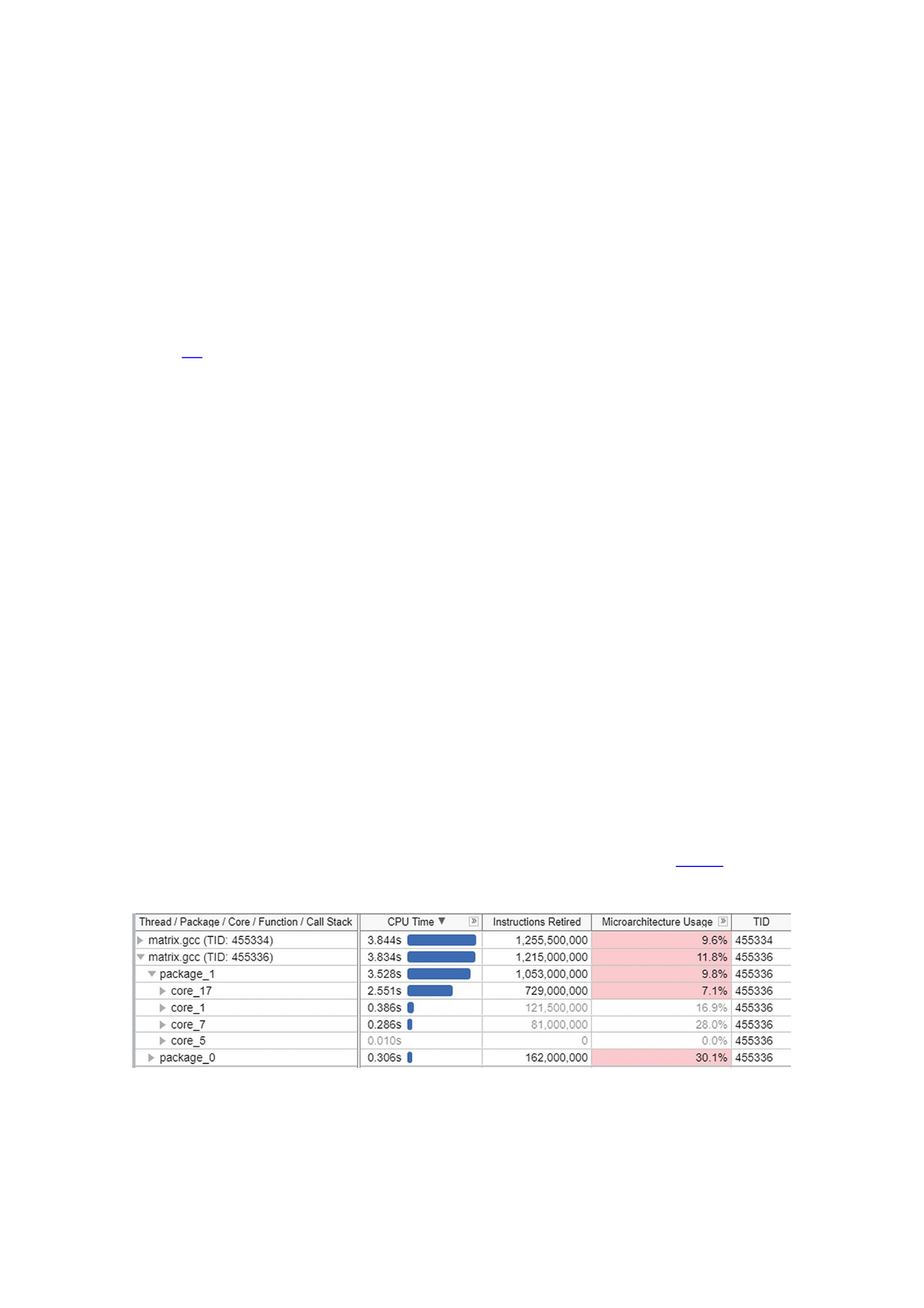
performance issues related to NUMA memory accesses, two things should be

considered: data allocation vs. first access, and thread migration.

Data Allocation vs. First Access

Data allocation is the process of allocating or reserving some amount of virtual

address space for an object. The virtual address space for a process is the set of virtual

memory addresses that it can use. The address space for each process is private and

cannot be accessed by other processes unless it is shared. A virtual address does not

represent the actual physical location of an object in memory. Instead, the system

maintains a multilayered page table, which is an internal data structure used to

translate virtual addresses into their corresponding physical addresses. Each time an

application thread references an address, the system translates the virtual address to a

physical address. The physical address points to memory physically connected to a CPU.

Chapter 19 describes exactly how this operation works and shows why high-capacity

memory systems can benefit from using large or huge pages provided by the operating

system.

A common practice in software is to have most of the data allocations done when the

application starts. Operating systems try to allocate memory associated with the CPU on

which the thread executes. The operating system scheduler then tries to always

schedule the thread on a CPU that it last ran in the hopes that the data still remains in

one of the CPU caches. On a multi-socket system, this may result in all the objects being

allocated in the memory of a single socket, which can create NUMA performance issues.

Accessing data on a remote CPU incurs a latency performance penalty.

Some applications delay reserving memory until the data is accessed for the first

time. This can alleviate some NUMA issues. It is important to understand how your

workload allocates data to understand the NUMA performance.

Thread Migration

Thread migration , which is the movement of software threads across sockets by the

operating system scheduler, is the most common cause of NUMA issues. Once objects

are allocated in memory, accessing them from another physical CPU from which they

were originally allocated incurs a latency penalty. Even though you may allocate your

data on a socket where the accessing thread is currently running, unless you have

specific affinity bindings or other safeguards, the thread may move to any other core or

socket in the future. You can track thread migration by identifying which cores threads

are running on and which sockets those cores belong to. Figure 15-10 shows an

example of this analysis from VTune Profiler.

Figure 15-10VTune Profiler identifying thread migration across cores and sockets (packages)

Use this information to determine whether thread migration is correlated with

NUMA accesses to remote DRAM or persistent memory.

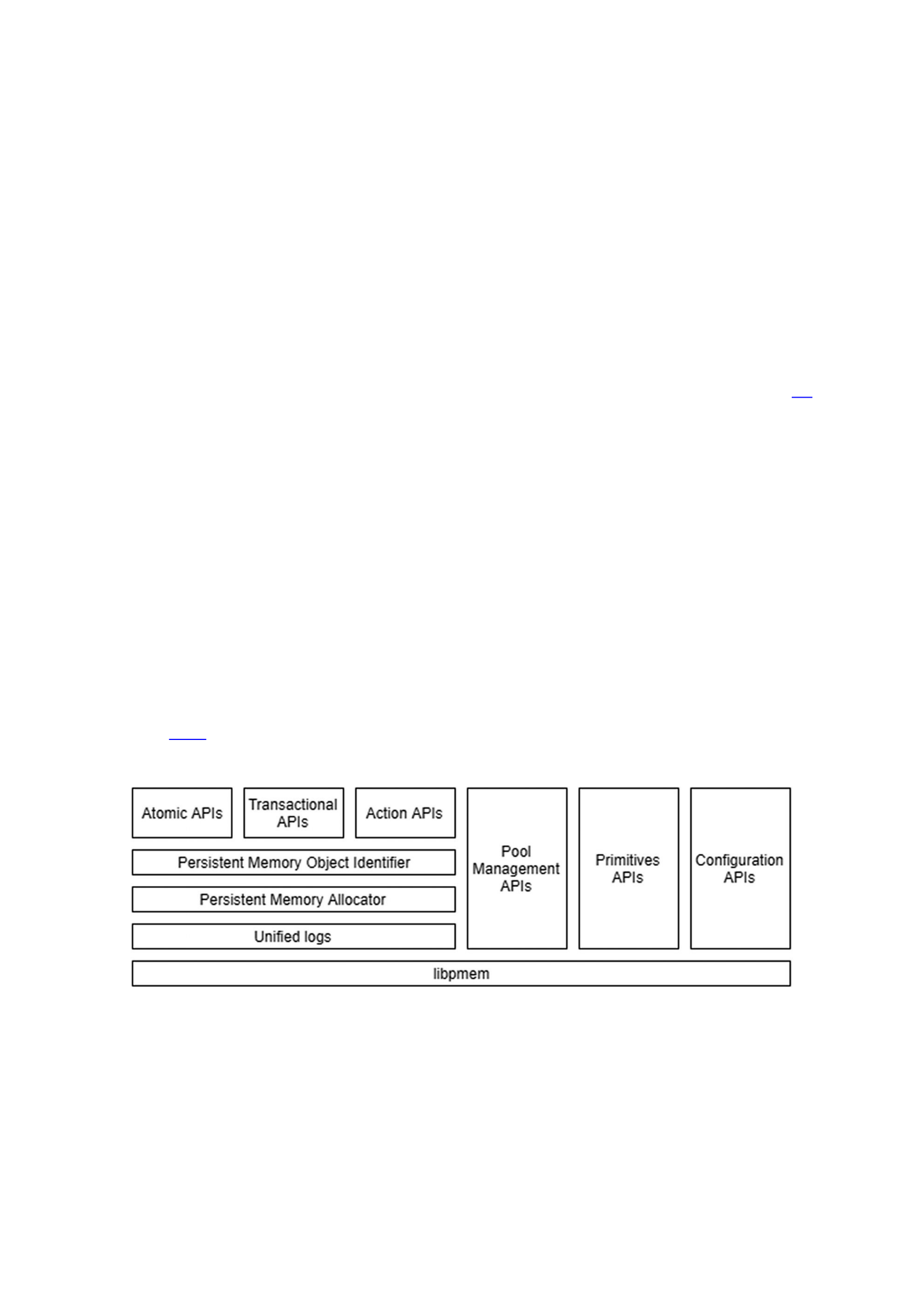
Large and Huge Pages

The default memory page size in most operating systems is 4 kilobytes (KiB).

Operating systems provide many different page sizes for different application

workloads and requirements. In Linux, a Large Page is 2 megabytes (MiB), and a Huge

Page is 1 gigabyte (GiB). The larger page sizes can be beneficial to workload

performance on persistent memory in certain scenarios.

For applications with a large addressable memory requirement, the size of the page

table being maintained by the operating system for virtual to physical address

translation grows significantly larger in size. The translation lookaside buffer (TLB) is a

small cache to make virtual-to-physical address translations faster. The efficiency of

TLB goes down when the number of page entries increases in the page table. Chapter 19

describes this in more detail.

Persistent memory systems that are meant for applications with a large memory

requirement will likely encounter the problem of large page tables and inefficient TLB

usage. Using large page sizes in this scenario helps reduce the number of entries in the

page table. The main trade-offs when using large page sizes is a higher overhead for

each allocation and memory fragmentation. You must be aware of the application

behavior before using large pages on persistent memory. An application doing frequent

allocation/deallocation may not be a good fit for large page optimization. The memory

fragmentation issue is somewhat abated by the large address space available on the

persistent memory systems.

A Pool of Persistent Memory: High-Level Architecture

Overview

Figure 16-1 shows that libpmemobj comprises many isolated components that build

on top of each other to provide a transactional object store.

Figure 16-1The modules of the libpmemobj architecture

Everything is built on top of libpmem and its persistence primitives that the library

uses to transfer data to persistent memory and persist it. Those primitives are also

exposed through libpmemobj-specific APIs to applications that wish to perform low-

level operations on persistent memory, such as manual cache flushing. These APIs are

exposed so the high-level library can instrument, intercept, and augment all stores to

persistent memory. This is useful for the instrumentation of runtime analysis tools such

as Valgrind pmemcheck, described in Chapter 12. More importantly, these functions are

interception points for data replication, both local and remote.

Replication is implemented in a way that ensures all data written prior to calling

drain will be safely stored in the replica as configured. A drain operation is a barrier

that waits for hardware buffers to complete their flush operation to ensure all writes

have reached the media. This works by initiating a write to the replica when a memory

copy or a flush is performed and then waits for those writes to finish in the drain call.

This mechanism guarantees the same behavior and ordering semantics for replicated

and non-replicated pools.

On top of persistence primitives provided by libpmem is an abstraction for fail-safe

modification of transactional data called unified logging. The unified log is a single data

structure and API for two different logging types used throughout libpmemobj to

ensure fail-safety: transactions and atomic operations. This is one of the most crucial,

performance-sensitive modules in the library because it is the hot code path of almost

every API. The unified log is a hybrid DRAM and persistent memory data structure

accessed through a runtime context that organizes all memory operations that need to

be performed within a single fail-safe atomic transaction and allows for critical

performance optimizations.

The persistent memory allocator operates in the unified log context of either a

transaction or a single atomic operation. This is the largest and most complex module in

libpmemobj and is used to manage the potentially large amounts of persistent

memory associated with the memory pool.

Each object stored in a persistent memory pool is represented by an object handle of

type PMEMoid (persistent memory object identifier). In practice, such a handle is a

unique object identifier (OID) of global scope, which means that two objects from

different pools will never have the same OID. An OID cannot be used as a direct pointer

to an object. Each time the program attempts to read or write object data, it must obtain

the current memory address of the object by converting its OID into a pointer. In

contrast to the memory address, the OID value for a given object does not change during

the life of an object, except for a realloc(), and remains valid after closing and

reopening the pool. For this reason, if an object contains a reference to another

persistent object, for example, to build a linked data structure, the reference must be an

OID and not a memory address.

The atomic and transactional APIs are built using a combination of the persistent

memory allocator and unified logs. The simplest public interface is the atomic API which

runs a single allocator operation in a unified log context. That log context is not exposed

externally and is created, initialized, and destroyed within a single function call.

The most general-purpose interface is the transactional API, which is based on a

combination of undo logging for snapshots and redo logging for memory allocation and

deallocation. This API has ACID (atomicity, consistency, isolation, durability) properties,

and it is a relatively thin layer that combines the utility of unified logs and the persistent

memory allocator.

For specific transactional use cases that need low-level access to the persistent

memory allocator, there is an “action” API. The action API is essentially a pass-through

to the raw memory allocator interface, alongside helpers for usability. This API can be

leveraged to create low-overhead algorithms that issue fewer memory fences, as

compared to general-purpose transactions, at the cost of ease of use.

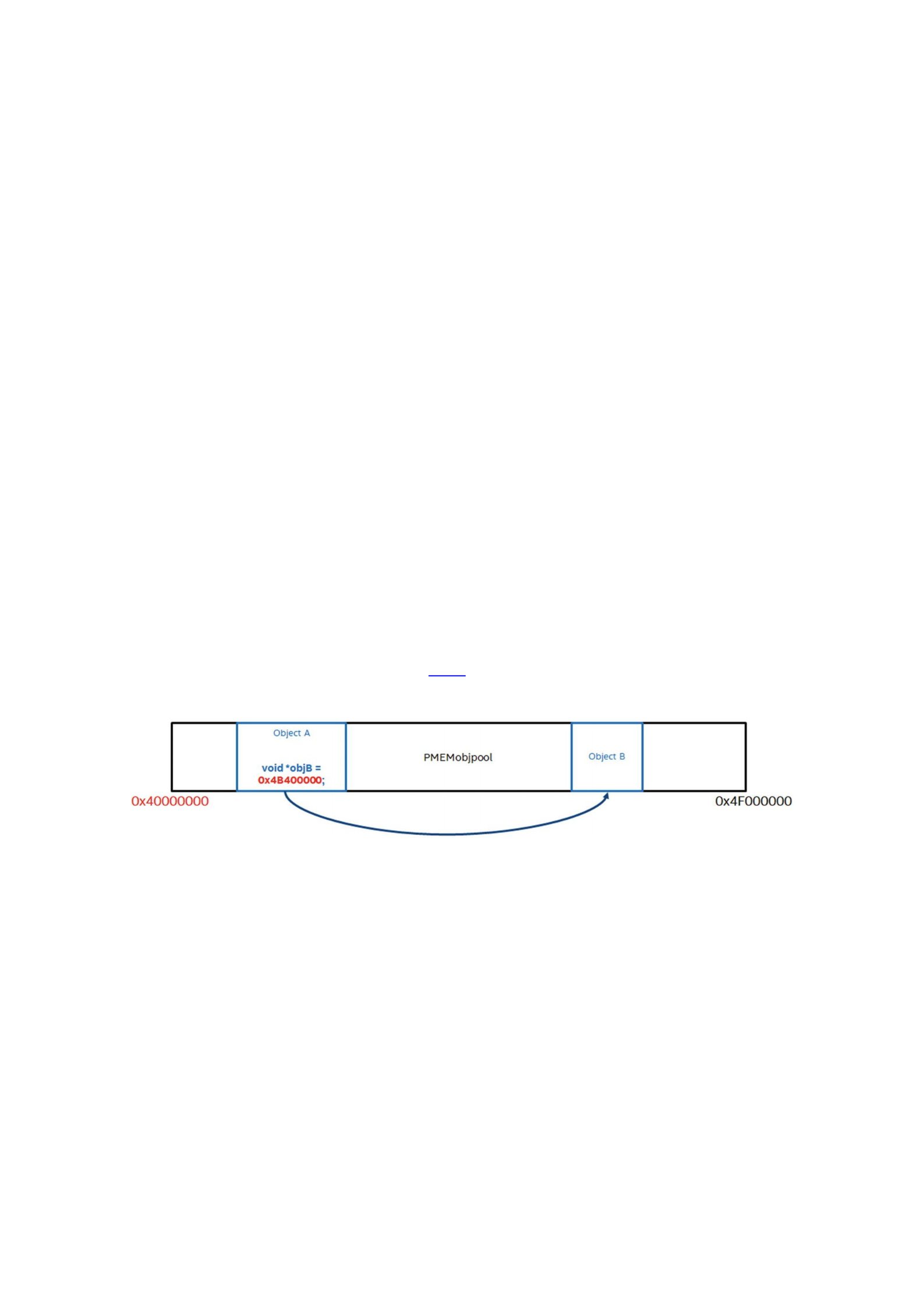
All public interfaces produce and operate on PMEMoids as a replacement for

pointers. This comes with space overhead because PMEMoids are 16 bytes. There is also

a performance overhead for the translation to a normal pointer. The upside is that

objects can be safely referenced between different instances of the application and even

different persistent memory pools.

The pool management API opens, maps, and manages persistent memory resident

files or devices. This is where the replication is configured, metadata and the heap are

initialized, and all the runtime data is created. This is also where the crucial recovery of

interrupted transactions happens. Once recovery is complete, all prior transactions are

either committed or aborted, the persistent state is consistent, and the logs are clean

and ready to be used again.

The Uncertainty of Memory Mapping: Persistent Memory

Object Identifier

A key concept that is important for any persistent memory application is how to

represent the relative position of an object within a pool of memory, and even beyond it.

That is, how do you implement pointers? You could rely on normal pointers, which are

relative to the beginning of the application’s virtual address space, but that comes with

many caveats. Using such pointers would be predicated on the pool of persistent

memory always being located at the same place in the virtual address space of an

application that maps it. This is difficult, if not impossible, to accomplish in a portable

way on modern operating systems due to address space layout randomization (ASLR) .

Therefore, a general-purpose library for persistent memory programming must provide

a specialized persistent pointer. Figure 16-2 shows a pointer from Object A to Object B.

If the base address changes, the pointer no longer points to Object B.

Figure 16-2Example of using a normal pointer in a persistent memory pool

An implementation of a general-purpose relative persistent pointer should satisfy

these two basic requirements:

The pointer must remain valid across application restarts.

2. The pointer should unambiguously identify a memory location in the presence of

many persistent memory pools, even if not located in a pool from which it was

originally derived.

In addition to the previous requirements, you should also consider some potential

performance problems:

Additional space overhead over a traditional pointer. This is important

because large fat pointers would take up more space in memory and because

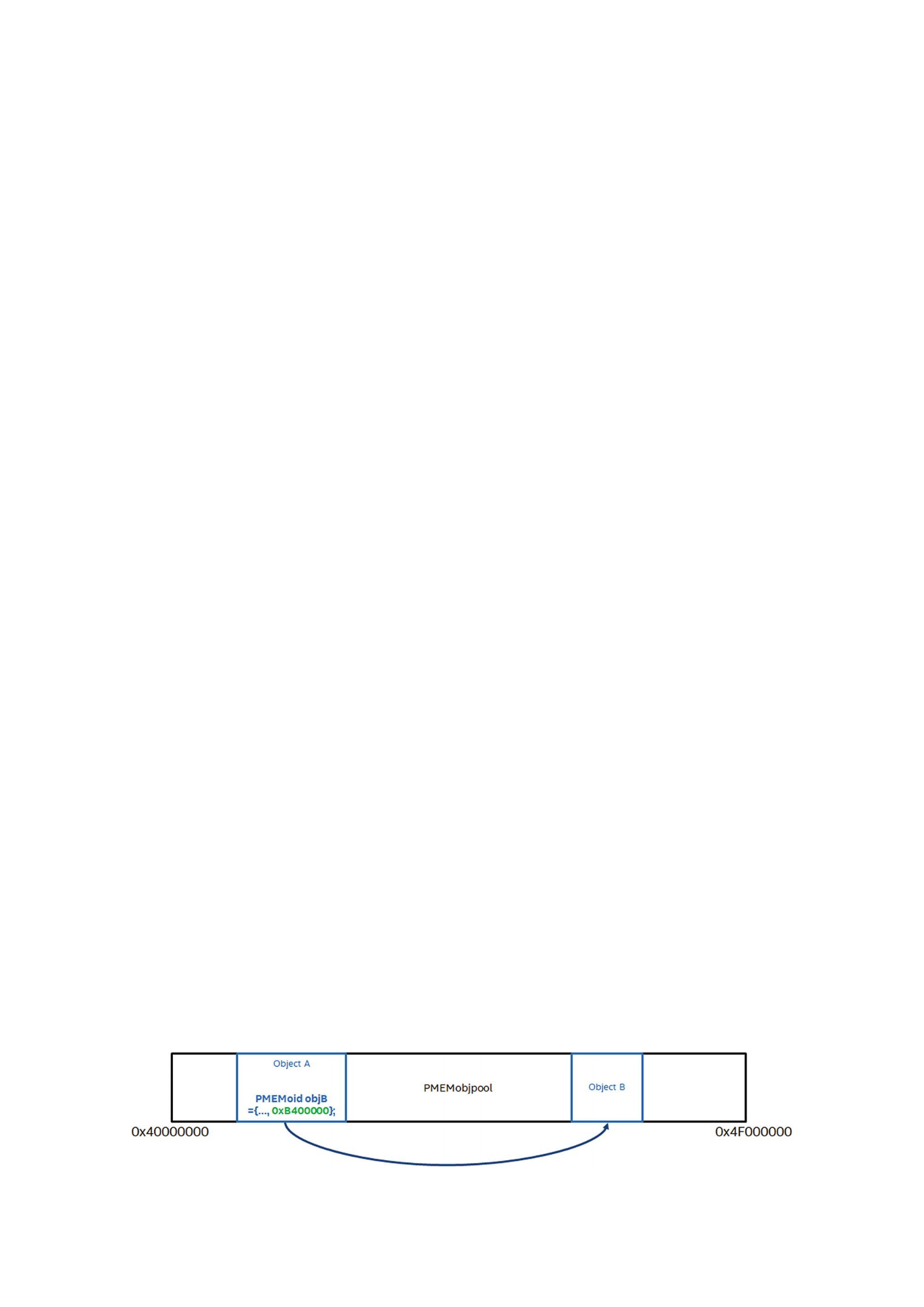
fewer of these fat pointers would fit in a single CPU cache line. This

potentially increases the cost of operations in pointer-chasing heavy data

structures, such as those found in B-tree algorithms.

The cost of translating persistent pointers to real pointers. Because

dereferencing is an extremely common operation, this calculation must be as

lightweight as possible and should involve as few instructions as possible.

This is to ensure that persistent pointer usage is efficient and it doesn’t

generate too much code bloat during compilation.

Preventing compiler optimizations through the dereferencing method. A

complicated pointer translation might negatively impact the compiler’s

optimization passes. The translation method should ideally avoid operations

that depend on an external state because that will prevent, among other

things, auto-vectorization.

Satisfying the preceding requirements while maintaining low-overhead and C99

standard compliance is surprisingly difficult. We explored several options:

The 8-byte offset pointer, relative to the beginning of the pool, was quickly

ruled out because it did not satisfy the second requirement and needed a

pool base pointer to be provided to the translation method.

8-byte self-relative pointers, where the value of the pointer is the offset

between the object’s location and the pointer’s location. This is potentially

the fastest implementation because the translation method can be

implemented as `ptr + (*ptr)`. However, this does not satisfy the

second basic requirement. Additionally, it would require a special

assignment method because the value of the pointer to the same object

would differ depending on the pointer’s location.

8-byte offset pointers with embedded memory pool identifier, which allows

the library to satisfy the second requirement. This is an augmentation of the

first method that additionally stores the identifier in the unused part of the

pointer value by taking advantage of the fact that the usable size of the

virtual address space is smaller than the size of the pointer on most modern

CPUs. The problem with this method, however, is that the number of bits for

the pool identifier is relatively small (16 bits on modern CPUs) and might

shrink with future hardware.

16-byte fat offset pointer with pool identifier. This is the most obvious

solution, which is similar to the one earlier but has 8-byte offset pointers and

8-byte pool identifiers. Fat pointers provide the best utility, at the cost of

space overhead and some runtime performance.

libpmemobj uses the most generic approach of the 16-byte offset pointer. This

allows you to make your own choice since all other pointer types can be directly derived

from it. libpmemobj bindings for more expressive languages than C99, such as C++,

can also provide different types of pointers with different trade-offs.

Figure 16-3Example of using a PMEMoid in a persistent memory pool

Figure 16-3 shows the translation method used to convert a libpmemobj

persistent pointer, PMEMoid, into a valid C pointer. In principle, this approach is very

simple. We look up the base address of the pool through the pool identifier and then add

the object offset to it. The method itself is static inline and defined in the public header

file for libpmemobj to avoid a function call on every deference. The problem is the

lookup method, which, for an application linked with a dynamic library, means a call to

a different compilation unit, and that might be costly for a very commonly performed

operation. To resolve this problem, the translation method has a per-thread cache of the

last base address, which removes the necessity of calling the lookup with each

dereferencing for the common case where persistent pointers from the same pool are

accessed close together.

The pool lookup method itself is implemented using a radix tree that stores

identifier-address pairs. This tree has a lock-free read operation, which is necessary

because each non-cached pointer translation would otherwise have to acquire a lock to

be thread-safe, and that would have a severe negative performance impact and could

potentially serialize access to persistent memory.

Persistent Thread Local Storage: Using Lanes

Very early in the development of PMDK, we found that persistent memory

programming closely resembles multithreaded programming because it requires

restricting visibility of memory changes – either through locking or transactions – to

other threads or instances of the program. But that is not the only similarity. The other

similarity, which we discuss in this section, is how sometimes low-level code needs to

store data that is unique to one thread of execution. In the persistent case, we often

need to associate data with a transaction rather than a thread.

In libpmemobj, we need a way to create an association between an in-flight

transaction and its persistent logs. It also requires a way to reconnect to those logs after

an unplanned interruption. The solution is to use a data structure called a “lane,” which

is simply a persistent byte buffer that is also transaction local.

Lanes are limited in quantity, have a fixed size, and are located at the beginning of

the pool. Each time a transaction starts, it chooses one of the lanes to operate from.

Because there is a limited number of lanes, there is also a limited number of

transactions that can run in parallel. For this reason, the size of the lane is relatively

small, but the number of lanes is big enough as to be larger than a number of application

threads that could feasibly run in parallel on current platforms and platforms coming in

the foreseeable future.

The challenge of the lane mechanism is the selection algorithm, that is, which lane to

choose for a specific transaction. It is a scheduler that assigns resources (lanes) to

perform work (transactions).

The naive algorithm, which was implemented in the earliest versions of

libpmemobj, simply picked the first available lane from the pool. This approach has a

few problems. First, the implementation of what effectively amounts to a single LIFO

(last in, first out) data structure of lanes requires a lot of synchronization on the front of

the stack, regardless of whether it is implemented as a linked list or an array, and thus

reducing performance. The second problem is false sharing of lane data. False sharing

occurs when two or more threads operate on data that is being modified, causing CPU

cache thrashing. And that is exactly what happens if multiple threads are continually

fighting over the same number of lanes to start new transactions. The third problem is

spreading the traffic across interleaved DIMMs. Interleaving is a technique that allows

sequential traffic to take advantage of throughput of all of the DIMMs in the interleave

set by spreading the physical memory across all available DIMMs. This is similar to

striping (RAID0) across multiple disk drives. Depending on the size of the interleaved

block, and the platform configuration, using naive lane allocation might continuously

use the same physical DIMMs, lowering the overall performance.

To alleviate these problems, the lane scheduling algorithm in libpmemobj is more

complex. Instead of using a LIFO data structure, it uses an array of 8-byte spinlocks, one

for each lane. Each thread is initially assigned a primary lane number, which is assigned

in such a way as to minimize false sharing of both lane data and the spinlock array. The

algorithm also tries to spread the lanes evenly across interleaved DIMMs. As long as

there are fewer active threads than lanes, no thread will ever share a lane. When a

thread attempts to start a transaction, it will try to acquire its primary lane spinlock,

and if it is unsuccessful, it will try to acquire the next lane in the array.

The final lane scheduling algorithm decision took a considerable amount of research

into various lane scheduling approaches. Compared to the naive implementation, the

current implementation has vastly improved performance, especially in heavily

multithreaded workloads.

Ensuring Power-Fail Atomicity: Redo and Undo Logging

The two fundamental concepts libpmemobj uses to ensure power-fail safety are

redo and undo logging. Redo logs are used to ensure atomicity of memory allocations,

while undo logs are used to implement transactional snapshots. Before we discuss the

many different possible implementation approaches, this section describes the basic

ideas.

Transaction Redo Logging

Redo logging is a method by which a group of memory modifications that need to be

done atomically are stored in a log and deferred until all modifications in the group are

persistently stored. Once completed, the log is marked as complete, and the memory

modifications are processed (applied); the log can then be discarded. If the processing is

interrupted before it finishes, the logging is repeated until successful. Figure 16-4 shows

the four phases of transaction redo logging.

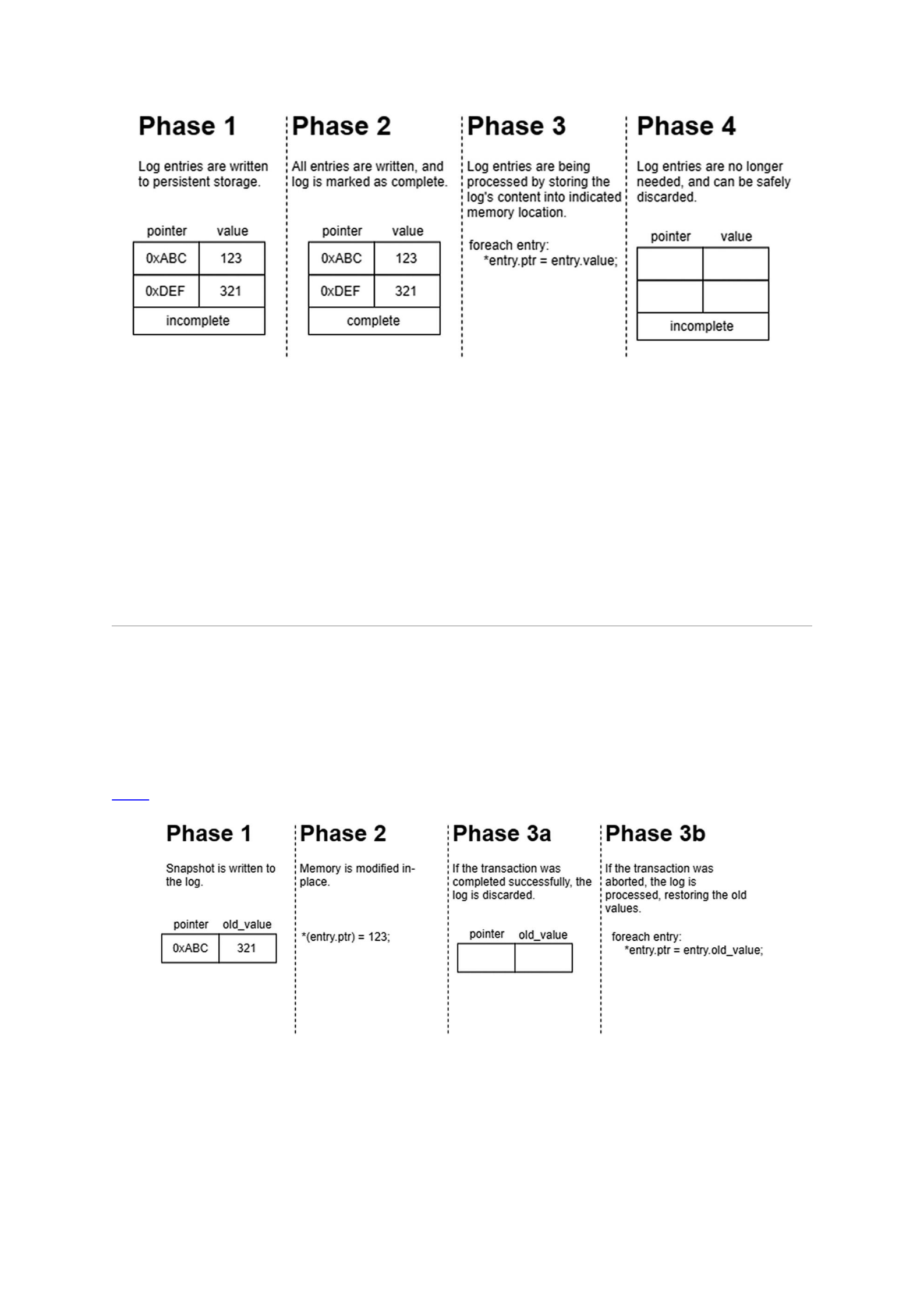
Figure 16-4The phases of a transaction redo log

The benefit of this logging approach, in the context of persistent memory, is that all

the log entries can be written and flushed to storage at once. An optimal

implementation of redo logging uses only two synchronization barriers: once to mark

the log as complete and once to discard it. The downside to this approach is that the

memory modifications are not immediately visible, which makes for a more

complicated programming model. Redo logging can sometimes be used alongside

load/store instrumentation techniques which can redirect a memory operation to the

logged location. However, this approach can be difficult to implement efficiently and is

not well suited for a general-purpose library.

Transaction Undo Logging

Undo logging is a method by which each memory region of a group (undo transaction)

that needs to be modified atomically is snapshotted into a log prior to the modification.

Once all memory modifications are complete, the log is discarded. If the transaction is

interrupted, the modifications in the log are rolled back to their original state. Figure

16-5 shows the three phases of the transaction undo logging.

Figure 16-5Phases of a transaction undo log

This type of log can have lower performance characteristics compared with the redo

log approach because it requires a barrier for every snapshot that needs to be made,

and the snapshotting itself must be fail-safe atomic, which presents its own challenges.

An undo log benefit is that the changes are visible immediately, allowing for a natural

programming model.

The important observation here is that redo and undo logging are complimentary.

Use redo logging for performance-critical code and where deferred modifications are

not a problem; use undo logging where ease of use is important. This observation led to

the current design of libpmemobj where a single transaction takes advantage of both

algorithms.

libpmemobj Unified Logging

Both redo and undo logging in libpmemobj share the same internal interface and

data structure, which is called a unified log (or ulog for short). This is because redo and

undo logging only differ in the execution order of the log phases, or more precisely,

when the log is applied on commit or recovery. In practice, however, there are

performance considerations that require specialization in certain parts of the algorithm.

The ulog data structure contains one cache line header with metadata and a variable

length array of data bytes. The header consists of:

A checksum for both the header and data, used only for redo logs

A monotonically increasing generation number of a transaction in the log,

used only for undo logs

The total length in bytes of the data array

An offset of the next log in the group

The last field is used to create a singly linked list of all logs that participate in a single

transaction. This is because it is impossible to predict the total required size of the log at

the beginning of the transaction, so the library cannot allocate a log structure that is the

exact required length ahead of time. Instead, the logs are allocated on demand and

atomically linked into a list.

The unified log supports two ways of fail-safe inserting of entries:

Bulk insert takes an array of log entries, prepares the header of the log, and creates

a checksum of both the header and data. Once done, a non-temporal copy, followed

by a fence, is performed to store this structure into persistent memory. This is the

way in which a group of deferred memory modifications forms a redo log with only

one additional barrier at the end of the transaction. In this case, the checksum in the

header is used to verify the consistency of the entire log. If that checksum doesn’t

match, the log is skipped during recovery.

2. Buffer insert takes only a single entry, checksums it together with the current

generation number, and stores it in persistent memory through non-temporal stores

followed by a fence. This method is used to create undo logs when snapshotting.

Undo logs in a transaction are different than redo logs because during the commit’s

fast path, they need to be invalidated instead of applied. Instead of laboriously

writing zeros into the log buffer, the log is invalidated by incrementing the

generation number. This works because the number is part of the data with its

checksum, so changing the generation number will cause a checksum failure. This

algorithm allows libpmemobj to have only one additional fence for the transaction

(on top of the fences needed for snapshots) to ensure fail-safety of a log, resulting in

very low-overhead transactions.

Persistent Allocations: The Interface of a Transactional

Persistent Allocator

The internal allocator interface in libpmemobj is far more complex than a typical

volatile dynamic memory allocator. First, it must ensure fail-safety of all its operations

and cannot allow for any memory to become unreachable due to interruptions. Second,

it must be transactional so that multiple operations on the heap can be done atomically

alongside other modifications. And lastly, it must operate on the pool state, allocating

memory from specific files instead of relying on the anonymous virtual memory

provided by the operating system. All these factors contribute to an internal API that

hardly resembles the standard malloc() and free(), shown in Listing 16-1.

int palloc_reserve(struct palloc_heap *heap, size_t size,...,

struct pobj_action *act);

void palloc_publish(struct palloc_heap *heap,

struct pobj_action *actv, size_t actvcnt,

struct operation_context *ctx);

Listing 16-1The core persistent memory allocator interface that splits heap operations into two distinct steps

All memory operations, called “actions” in the API, are broken up into two individual

steps.

The first step reserves the state that is needed to perform the operation. For

allocations, this means retrieving a free memory block, marking it as reserved, and

initializing the object’s content. This reservation is stored in a user-provided runtime

variable. The library guarantees that if an application crashes while holding

reservations, the persistent state is not affected. That is why these action variables must

not be persistent.

The second step is the act of exercising the reservations, which is called

“publication.” Reservations can be published individually, but the true power of this API

lies in its ability to group and publish many different actions together.

The internal allocator API also has a function to create an action that will set a

memory location to a given value when published. This is used to modify the destination

pointer value and is instrumental in making the atomic API of libpmemobj fail-safe.

All internal allocator APIs that need to perform fail-safe atomic actions take

operation context as an argument, which is the runtime instance of a single log. It

contains various state information, such as the total capacity of the log and the current

number of entries. It exposes the functions to create either bulk or singular log entries.

The allocator’s functions will log and then process all metadata modifications inside of

the persistent log that belongs to the provided instance of the operating context.

Persistent Memory Heap Management: Allocator Design

for Persistent Memory

The previous section described the interface for the memory allocation used

internally in libpmemobj, but that was only the tip of the allocator iceberg. Before

diving deeper into this topic, we briefly describe the principles behind normal volatile

allocators so you can understand how persistent memory impacts the status quo.

Traditional allocators for volatile memory are responsible for efficient – in both time

and space – management of operating system–provided memory pages. Precisely how

this should be done for the generic case is an active research area of computer science;

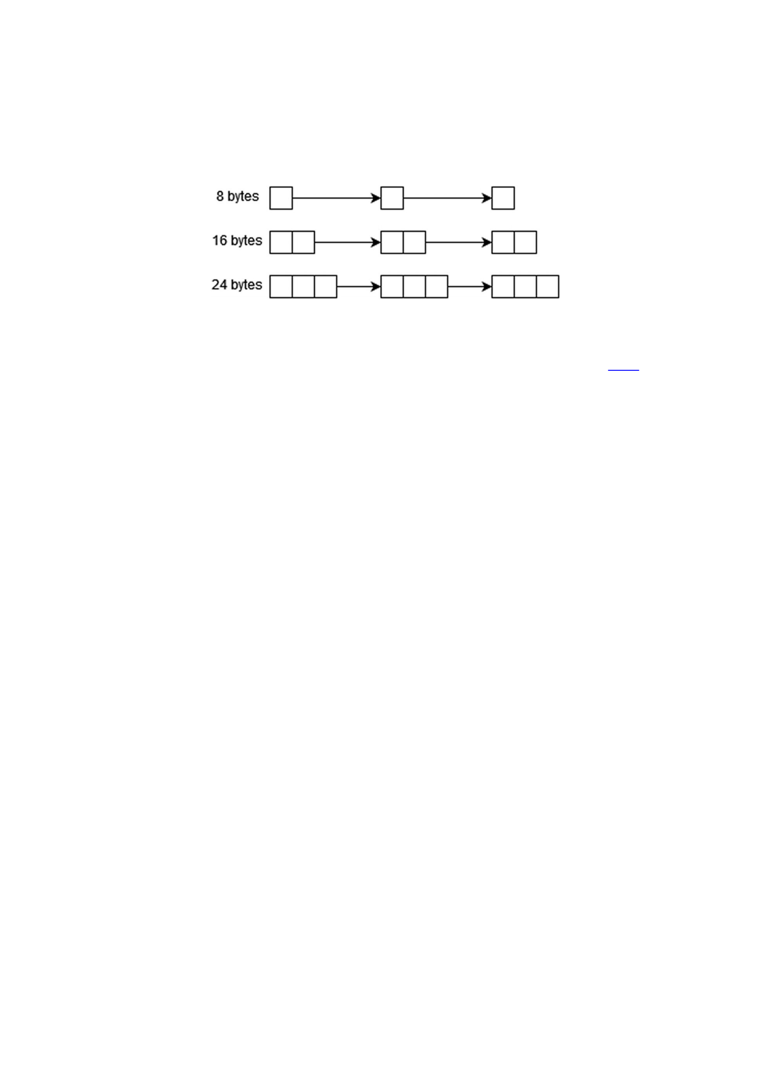
many different techniques can be used. All of them try to exploit the regularities in

allocation and deallocation patterns to minimize heap fragmentation.

Most commonly used general-purpose memory allocators settled on an algorithm

that we refer to as “segregated fit with page reuse and thread caching.”

Figure 16-6Example of free lists in a memory allocator

This works by using a free list for many different sizes, shown in Figure 16-6, until

some predefined threshold, after which it is sensible to allocate directly from the

operating system. Those free lists are typically called bins or buckets and can be

implemented in various ways, such as a simple linked list or contiguous buffer with

boundary tags. Each incoming memory allocation request is rounded up to match one of

the free lists, so there must be enough of them to minimize the amount of

overprovisioned space for each allocation. This algorithm approximates a best-fit

allocation policy that selects the memory block with the least amount of excess space

for the request from the ones available.

Using this technique allows memory allocators to have average-case O(1)

complexity while retaining the memory efficiency of best fit. Another benefit is that

rounding up of memory blocks and subsequent segregation forces some regularity to

allocation patterns that otherwise might not exhibit any.

Some allocators also sort the available memory blocks by address and, if possible,

allocate the one that is spatially collocated with previously selected blocks. This

improves space efficiency by increasing the likelihood of reusing the same physical

memory page. It also preserves temporal locality of allocated memory objects, which

can minimize cache and translation lookaside buffer (TLB) misses.

One important advancement in memory allocators is scalability in multithreaded

applications. Most modern memory allocators implement some form of thread caching,

where the vast majority of allocation requests are satisfied directly from memory that is

exclusively assigned to a given thread. Only when memory assigned to a thread is

entirely exhausted, or if the request is very large, the allocation will contend with other

threads for operating system resources.

This allows for allocator implementations that have no locks of any kind, not even

atomics, on the fast path. This can have a potentially significant impact on performance,

even in the single-threaded case. This technique also prevents allocator-induced false

sharing between threads, since a thread will always allocate from its own region of

memory. Additionally, the deallocation path often returns the memory block to the

thread cache from which it originated, again preserving locality.

We mentioned earlier that volatile allocators manage operating system–provided

pages but did not explain how they acquire those pages. This will become very

important later as we discuss how things change for persistent memory. Memory is

usually requested on demand from the operating system either through sbrk() , which

moves the break segment of the application, or anonymous mmap(), which creates new

virtual memory mapping backed by the page cache. The actual physical memory is

usually not assigned until the page is written to for the first time. When the allocator

decides that it no longer needs a page, it can either completely remove the mapping

using unmap() or it can tell the operating system to release the backing physical pages

but keep the virtual mapping. This enables the allocator to reuse the same addresses

later without having to memory map them again.

How does all of this translate into persistent memory allocators and libpmemobj

specifically?

The persistent heap must be resumable after application restart. This means that all

state information must be either located on persistent memory or reconstructed on

startup. If there are any active bookkeeping processes, those need to be restarted from

the point at which they were interrupted. There cannot be any volatile state held in

persistent memory, such as thread cache pointers. In fact, the allocator must not

operate on any pointers at all because the virtual address of the heap can change

between restarts.

In libpmemobj, the heap is rebuilt lazily and in stages. The entire available

memory is divided into equally sized zones (except for the last one, which can be

smaller than the others) with metadata at the beginning of each one. Each zone is

subsequentially divided into variably sized memory blocks called chunks. Whenever

there is an allocation request, and the runtime state indicates that there is no memory

to satisfy it, the zone’s metadata is processed, and the corresponding runtime state is

initialized. This minimizes the startup time of the pool and amortizes the cost of

rebuilding the heap state across many individual allocation requests.

There are three main reasons for having any runtime state at all. First, access latency

of persistent memory can be higher than that of DRAM, potentially impacting

performance of data structures placed on it. Second, separating the runtime state from

the persistent state enables a workflow where the memory is first reserved in runtime

state and initialized, and only then the allocation is reflected on the persistent state.

This mechanism was described in the previous section. Finally, maintaining fail-safety

of complex persistent data structures is expensive, and keeping them in DRAM allows

the allocator to sidestep that cost.

The runtime allocation scheme employed by libpmemobj is segregated fit with

chunk reuse and thread caching as described earlier. Free lists in libpmemobj, called

buckets, are placed in DRAM and are implemented as vectors of pointers to persistent

memory blocks. The persistent representation of this data structure is a bitmap, located

at the beginning of a larger buffer from which the smaller blocks are carved out. These

buffers in libpmemobj, called runs, are variably sized and are allocated from the

previously mentioned chunks. Very large allocations are directly allocated as chunks.

Figure 16-7 shows the libpmemobj implementation.

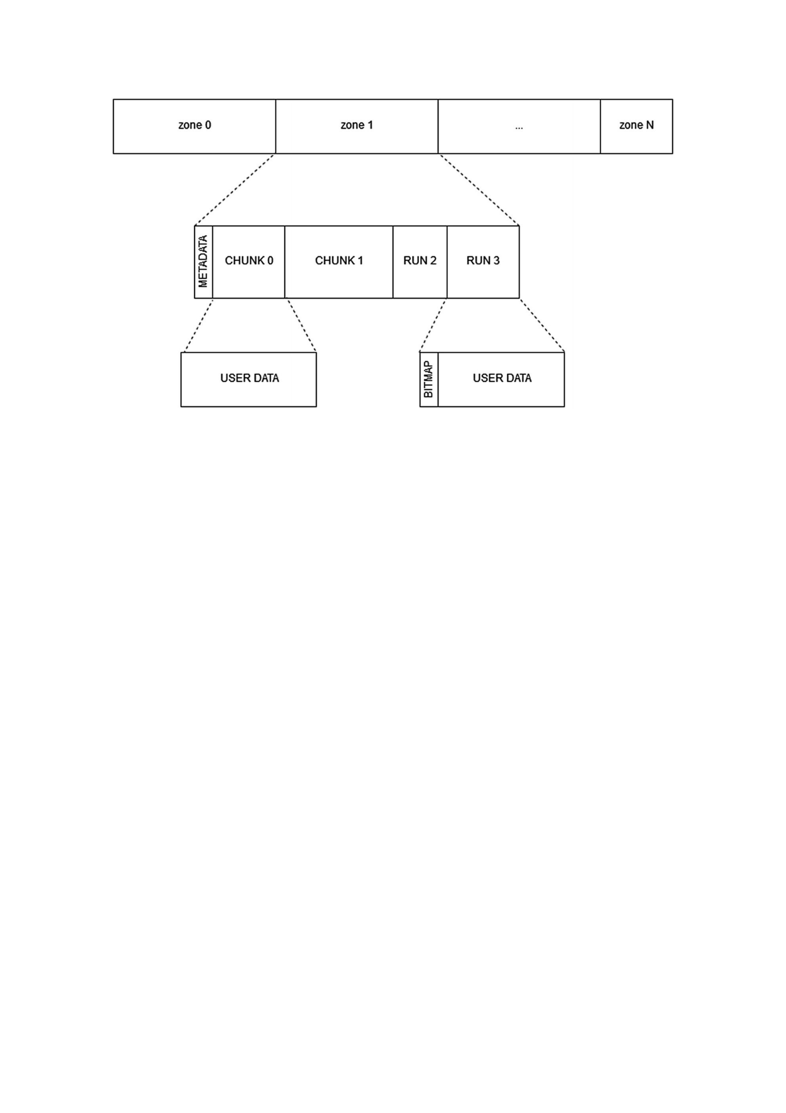
Figure 16-7On-media layout of libpmemobj’s heap

Persistent allocators must also ensure consistency in the presence of failures,

otherwise, memory might become unreachable after an ungraceful shutdown of the

application. One part of the solution is the API we outlined in the previous section. The

other part is the careful design of the algorithms inside the allocator that ensures no

matter when the application is aborted, the state is consistent. This is also aided by redo

logs, which are used to ensure atomicity of groups of noncontiguous persistent

metadata changes.

One of the most impactful aspects of persistent memory allocation is how the

memory is provisioned from the operating system. We previously explained that for

normal volatile allocators, the memory is usually acquired through anonymous memory

mappings that are backed by the page cache. In contrast, persistent heaps must use file-

based memory mappings, backed directly by persistent memory. The difference might

be subtle, but it has a significant impact on the way the allocator must be designed. The

allocator must manage the entire virtual address space, retain information about any

potential noncontiguous regions of the heap, and avoid excessive overprovisioning of

virtual address space. Volatile allocators can rely on the operating system to coalesce

noncontiguous physical pages into contiguous virtual ones, whereas persistent

allocators cannot do the same without explicit and complicated techniques.

Additionally, for some file system implementations, the allocator cannot assume that

the physical memory is allocated at the time of the first page fault, so it must be

conservative with internal block allocations.

Another problem for allocation from file-based mappings is that of perception.

Normal allocators, due to memory overcommitment, seemingly never run out of

memory because they are allocating the virtual address space, which is effectively

infinite. There are negative performance consequences of address space bloat, and

memory allocators actively try to avoid it, but they are not easily measurable in a typical

application. In contrast, memory heaps allocate from a finite resource, the persistent

memory device, or a file. This exacerbates the common phenomenon that is heap

fragmentation by making it trivially measurable, creating the perception that persistent

memory allocators are less efficient than volatile ones. They can be, but the operating

system does a lot of work behind the scene to hide fragmentation of traditional memory

allocators.

ACID Transactions: Efficient Low-Level Persistent

Transactions

The four components we just described – lanes, redo logs, undo logs, and the

transactional memory allocator – form the basis of libpmemobj's implementation of

ACID transactions that we defined in Chapter 4.

A transaction’s persistent state consists of three logs. First is an undo log, which

contains snapshots of user data. Second is an external redo log, which contains

allocations and deallocations performed by the user. Third is an internal redo log, which

is used to perform atomic metadata allocations and deallocations. This is technically not

part of the transaction but is required to allocate the log extensions if they are needed.

Without the internal redo log, it would be impossible to reserve and then publish a new

log object in a transaction that already had user-made allocator actions in the external

redo log.

All three logs have individual operation-context instances that are stored in runtime

state of the lanes. This state is initialized when the pool is opened, and that is also when

all the logs of the prior instance of the application are either processed or discarded.

There is no special persistent variable that indicates whether past transactions in the

log were successful or not. That information is directly derived from checksums stored

in the log.

When a transaction begins, and it is not a nested transaction, it acquires a lane,

which must not contain any valid uncomitted logs. The runtime state of the transaction

is stored in a thread-local variable, and that is where the lane variable is stored once

acquired.

Transactional allocator operations use the external redo log and its associated

operation context to call the appropriate reservation method which in turn creates an

allocator action to be published at the time of transaction commit. The allocator actions

are stored in a volatile array. If the transaction is aborted, all the actions are canceled,

and the associated state is discarded. The complete redo log for memory allocations is

created only at the time of transaction commit. If the library is interrupted while

creating the redo log, the next time the pool is opened, the checksum will not match, and

the transaction will be aborted by rolling back using the undo log.

Transactional snapshots use the undo log and its context. The first time a snapshot is

created, a new memory modification action is created in the external redo log. When

published, that action increments the generation number of the associated undo log,

invalidating its contents. This guarantees that if the external log is fully written and

processed, it automatically discards the undo log, committing the entire transaction. If

the external log is discarded, the undo log is processed, and the transaction is aborted.

To ensure that there are never two snapshots of the same memory location (this

would be an inefficient use of space), there is a runtime range tree that is queried every

time the application wants to create an undo log entry. If the new range overlaps with

an existing snapshot, adjustments to the input arguments are made to avoid duplication.

The same mechanism is also used to prevent snapshots of newly allocated data.

Whenever new memory in a transaction is allocated, the reserved memory range is

inserted into the ranges tree. Snapshotting new objects is redundant because they will

be discarded automatically in the case of an abort.

To ensure that all memory modifications performed inside the transaction are

durable on persistent memory once committed, the ranges tree is also used to iterate

over all snapshots and call the appropriate flushing function on the modified memory

locations.

Lazy Reinitialization of Variables: Storing the Volatile

State on Persistent Memory

While developing software for persistent memory, it is often useful to store the

runtime (volatile) state inside of persistent memory locations. Keeping that state

consistent, however, is extremely difficult, especially in multithreaded applications.

The problem is the initialization of the runtime state. One solution is to simply

iterate over all objects at the start of the application and initialize the volatile variables

then, but that might significantly contribute to startup time of applications with large

persistent pools. The other solution is to lazily reinitialize the variables on access, which

is what libpmemobj does for its built-in locks. The library also exposes this

mechanism through an API for use with custom algorithms.

Lazy reinitialization of the volatile state is implemented using a lock-free algorithm

that relies on a generation number stored alongside each volatile variable on persistent

memory and inside the pool header. The pool header resident copy is increased by two

every time a pool is opened. This means that a valid generation number is always even.

When a volatile variable is accessed, its generation number is checked against the one

stored in the pool header. If they match, it means that the object can be used and is

simply returned to the application; otherwise, the object needs to be initialized before

returning to ensure the initialization is thread-safe and is performed exactly once in a

single instance of the application.

The naive implementation could use a double-checked locking, where a thread

would try to acquire a lock prior to initialization and verify again if the generation

numbers match. If they still do not match, initialize the object, and increase the number.

To avoid the overhead that comes with using locks, the actual implementation first uses

a compare-and-swap to set the generation number to a value that is equal to the

generation number of the pool minus one, which is an odd number that indicates an

initialization operation is in progress. If this compare-and-swap were to fail, the

algorithm would loop back to check if the generation number matches. If it is successful,

the running thread initializes the variable and once again increments the generation

number – this time to an even number that should match the number stored in the pool

header.

Students also viewed