Introduction The Modular Open System Approach

General Issue

Congress and the DOD have long sought to improve the acquisition of major

weapon systems, yet many DOD programs are still falling short of cost, schedule,

and performance expectations. The results are unanticipated cost overruns,

reduced buying power, and in some cases delays or reductions in the capability

ultimately delivered to the warfighter.

Government Accountability Office, 2015 (GAO, 2015: 20)

The Modular Open System Approach (MOSA) was developed to help reverse the trend of

United States Department of Defense (DoD) weapons systems procurement programs

being delivered over budget and behind schedule. MOSA goes back as far as 1994, when

the original Open Systems Joint Task Force was created to "Sponsor and accelerate the

adoption of open systems in electronics included in weapons systems acquisitions,” in

order to “reduce life-cycle costs and facilitate effective weapon system intra- and

interoperability." (Kaminski, 1994: 1) Combining modular design and open architectures

with robust business practices, MOSA is intended to help deliver capability faster and

cheaper. The DoD has required the use of MOSA within the Defense Acquisition System,

in one form or another, for decades. However, not all programs have experienced the

promised effects of MOSA. Instead, costs have continued to rise and multiple major

weapons systems have seen their fielding delayed. Figure 1 highlights this trend by

showing the historical fielding times of various DoD systems, compared with other

technology intensive systems.

Figure 1: Trends for Acquisition Timelines in Software Intensive Systems

The Architecture Effect

Acquisition programs are chartered to deliver operationally useful systems to

satisfy a validated military need. To do this, programs balance many requirements to

design and deliver a weapon systems. MOSA is an approach that allows programs to

satisfy operational requirements using business practices to create an open system

implementation tailored to the program’s needs. An Open System is

A system that employs modular design tenets, uses widely supported and

consensus based standards for its key interfaces, and is subject to validation and

verification tests to ensure the openness of its key interfaces. (OSJTF, 2004: A3)

While not an exhaustive list, MOSA is supposed to:

• accelerate and simplify the delivery of advanced capability into systems

without replacing entire systems (Kendall, 2015: 14)

• provide valuable mechanisms for continuing competition and incremental

upgrades (DoD, 2015: 86)

• facilitate reuse across the joint force. (DoD, 2015: 86)

Despite this intent, DoD programs using MOSA have experienced varying levels

of success. Some have seen outstanding results, with cost reduced and fielding

accelerated. For example, the US Navy’s Acoustic Rapid COTS Insertion (ARCI)

program showed lifecycle cost improvements of 5 to 1. (Boudreau, 2009: xvi) However,

these success stories have proven to be the exception rather than the rule. Multiple major

programs have been born in the MOSA era, but the trend of over budget and late to need

programs has continued largely unchanged.

Unfulfilled Potential

Better Buying Power (BBP) 3.0 is an initiative written by the Under Secretary of

Defense for Acquisitions, Technology, and Logistics to “bend the cost curve.” (Kendall,

2015) It contains a series of guidelines for improving acquisition, one of which is

MOSA. BBP 3.0 outlines a primary challenge MOSA faces:

Often, this design feature has been either traded away because of competing

requirements or lost because the government has failed to secure technical control

and ownership of all the needed interfaces. (Kendall, 2015: 14)

The results of interviews conducted by the MOSA Technical Standards Working

Group (MOSA TSWG, 2016) indicate that program managers are not making a conscious

effort to acquire closed solutions. Instead, they are using MOSA, but making MOSA

implementation decisions that have negative consequences on their ability to cost

effectively modify their system. Through conversation with a variety of programs, it has

become clear that this is at least partially due to unclear or conflicting perception on how

these implementation decisions relate to the system’s operational utility, cost and

schedule. Programs believe that a completely closed solution is to be avoided because it

increases cost and schedule, and a completely open solution is ‘good’. In the author’s

opinion, rather than subscribe to these broad generalizations, programs that successfully

utilize MOSA trace particular architectural requirements to changes in specifically

defined operational utility for a given cost over the program’s life. Unsuccessful

programs sacrifice MOSA architecture requirements to meet immediate concerns, or

make architecture decisions that do not align with their business objectives. In either case,

the architectural implementation may be designed with MOSA principles, but not result

in lower cost or faster delivery.

Problem Statement

Despite application of MOSA guidance resulting in wildly different cost, schedule

and performance effects, DoD programs have no standardized methodology for

evaluating the lifecycle benefits of MOSA architecture alternatives. Insufficient analysis

results in programs making the same mistakes with a new architecture instead of realizing

the potential improvements of an architecture approach that embraces MOSA.

Developing a standardized methodology for evaluating the cost effectiveness of

architecture alternatives will help programs realize the MOSA benefits of greater utility,

reduced lifecycle cost, and decreased fielding time.

Research

The objective of this research is to address the problem discussed above by

answering the following primary research question:

Research Question:

How can programs evaluate the cost effectiveness of architecture alternatives

throughout the program lifecycle?

Investigative Questions

In order to fully address the primary research question, the following questions

will be systematically investigated:

Investigation Question 1

How are operational requirements defined and communicated?

Investigation Question 2

What is MOSA, and how are programs applying it?

Investigation Question 3

How can cost effectiveness for architectural decisions estimated throughout the

program lifecycle?

Investigation Question 4

How can operational utility be measured throughout the program lifecycle?

Investigation Question 5

How can the cost of MOSA be measured throughout the program lifecycle?

Methodology

The research presented in this paper proposes a framework for analyzing

architecture alternatives. The Architecture Cost Effectiveness Framework (ACEF)

directly evaluates how architecture choices affect operational utility and cost throughout

the lifecycle. These choices include the architecture requirements and any program

development increments. To do this, the ACEF compares two cost effectiveness ratios.

(1) The instantaneous cost effectiveness ratio, compares the operational utility to the total

cost at any point in the program. (2) The lifecycle cost effectiveness ratio, compares the

operational utility to the total cost for the entire lifecycle.

Operational utility is measured against the validated Key Performance Parameters

(KPPs) and Key System Attributes (KSAs) identified by the program and Additional

Performance Attributes (APAs) that the program office identifies. Multi-Attribute Utility

Analysis (MAUA) as primarily described by Keeney and Raiffa (Keeney and Raiffa,

1993) is used to aggregate the individual utilities associated with each KPP, KSA or APA

into a single operational utility value. To accomplish this, the program office develops an

Attribute Hierarchy based on the program’s required capabilities, with the leaf level

attributes corresponding to the program’s KPPs, KSAs and APAs. This hierarchy includes

weights for each leaf level attribute. Next, a lifecycle utility reference profile (LURP) is

developed for each leaf level attribute. A LURP is a set of utility curves that represent the

changing utility over time for that attribute. Each individual leaf level utility curve is

based on the threshold and objectives of the related KPP, KSA or APA. The LURPs are

documented in the program’s business plan.

Once the Attribute Hierarchy and LURPs are established, the program office

develops a reference architecture to communicate the desired architectural requirements

and creates multiple alternatives that comply with the reference architecture. Each

alternative includes a design implementation, as well as sufficient design increments to

address the business strategy of the alternative.

Once all alternatives have been generated, the cost effectiveness ratio is found for

each alternative. Operational utility is used as the effectiveness measure and is calculated

by applying the specific design choices for each alternative against the LURPs and

Attribute Hierarchy. To develop a measure of the utility over time, the utility is evaluated

annually. The cost is found by estimating the acquisition and integration cost of each

component. The Component Acquisition Cost is calculated by analogy to a known

component cost. The Component Integration Cost is calculated by using an appropriate

cost estimation tool to determine the changes required at each component interface. At

any point, the instantaneous cost effectiveness ratio can be evaluated for each alternative

by comparing the current annual utility and the cost to date. To evaluate the lifecycle cost

effectiveness ratio, the average annual utility is compared to the predicted total lifecycle

cost.

This analysis is performed multiple times to account for uncertainty in both the

analysis (due to user preference) and in the future combat environment (due to uncertain

predictions). The analyst should vary the weights provided in the Attribute Hierarchy to

determine the sensitivity of the analysis to user preference. The analyst should also vary

the LURPs throughout the lifecycle to understand how each alternative behaves in the

face of changing requirements. Finally, the results should be analyzed to determine how

the architectural decisions should change based on the cost effectiveness of the approach.

The last step in the process is to update the reference architecture and business plan based

on the predicted cost effectiveness shown by the analysis.

Assumptions

The research contained in this paper contains a variety of assumptions that are

necessary to scope the research. The first assumption is that the program office is able and

willing to develop a program roadmap of sufficient fidelity to scope requirement changes

throughout the program lifecycle. This includes developing LURPs that encompass future

requirement changes. This schedule will be vital to assessing the effectiveness of

architecture approaches. This assumption is challenging to meet, so additional sensitivity

analysis is performed regarding future requirements changes.

This analysis assumes that integration costs are able to be estimated by estimating

and summing the component acquisition and integration costs. The component

acquisition cost is based on existing systems with a modification factor applied to a

known cost for a current system. Ideally, components will be COTS, which tend to have

predictable lifecycle costs. Also, standard techniques for estimating costs of incrementally

improving IT components currently exist. Thus, cost estimates for evolutionary systems

should be acceptably accurate, but revolutionary systems may be less accurately

estimated using these techniques. Additionally, the cost estimating method does not

include global programmatic or engineering costs. These costs are assumed to be

equivalent between alternatives which should be valid when alternatives are roughly the

same magnitude. Future versions of the ACEF will utilize stochastic methods to account

for uncertainty in this cost estimation.

Limitations

The ACEF estimates cost by accounting for the component acquisition cost and

the component integration cost. The ACEF does not account for other costs, such as

maintenance of the architecture. Investigating how the maintenance cost of the

architecture alternatives affects the program is an area of future research. Additionally, the

component integration cost is calculated only for the software interfaces, and does not

encompass any hardware interfaces. This is another area that could be expanded in future

research.

Implications

The ACEF is targeted towards DoD program managers and will allow them to

understand how differing architecture alternatives deliver operational utility at a given

cost. This analysis facilitates traceability between the specific architecture decisions and

operational utility. This knowledge will allow the program manager to prioritize the

architectural requirements and then defend them over time. It is anticipated that this

knowledge will result in better realization of the benefits expected of MOSA application.

Preview

The remainder of this document is divided into four additional chapters. Chapter

II provides a review of the extant literature concerning: program requirements, MOSA

background, cost effectiveness analysis, multi-attribute utility analysis, and cost

estimation. Chapter III presents the analysis framework, including establishing the

business strategy with an Attribute Hierarchy and utility curves, development of a

reference architecture, the creation of alternatives, and the alternative comparison and

sensitivity analysis. Chapter IV describes the application of the methodology presented in

Chapter III, including a test case based on a notional weapon system. Finally, Chapter V

provides a discussion of the results, recommendations on their application, and future

research opportunities.

II. Literature Review

Chapter Overview

This chapter reviews the extant literature on a variety of topics, targeted towards

addressing the investigation questions posed in Chapter I. It begins with a discussion of

the Defense Acquisition System, focusing on how both capability and system

requirements are developed and documented. Next, MOSA is discussed, beginning with

an overview of the approach itself. MOSA acquisition tools are discussed, followed by an

overview of studies concerning MOSA implementation results. Next, cost effectiveness

analysis is discussed. Methods of calculating utility from multiple attributes are

investigated, including the development of attribute hierarchies and the additive value

function. Finally, there is a brief discussion of cost estimation, focusing on software costs.

The literature in this chapter forms the basis for the ACEF described in Chapters 3 and 4.

Acquisition Review

The Defense Acquisition System (DAS) manages the acquisition of weapon

systems to support the United States’ national security policy. The intended audience for

the ACEF is weapon systems programs, so this research assumes a basic level of

knowledge concerning the workings of the DAS. However, it is worth reinforcing some

important concepts. One major theme of DAS, as described in the primary governing

guidance for the DAS, Department of Defense Directive 5000.01, is that Program

Managers must tailor their programs to “satisfy user needs with measurable

improvements to mission capability and operational support, in a timely manner, and at a

fair and reasonable price.” (DoD, 2007: 3) Phrased a different way, program managers

must ensure that their solutions are cost effective (mission capability at a reasonable

cost), and that the timing of the capability delivery has value. To accomplish this, the

DAS prefers an incremental approach, meaning that the programs are planned and

executed to deliver capability in increments rather than in one step. This is intended to

deliver capability faster to the warfighter and allow future increments to be tailored to

lessons learned from earlier increments.

Capability Requirements

Before directing architectural requirements, the required weapon systems

capabilities must be understood. A capability requirement is a “capability which is

required to meet an organization’s roles, functions, and missions in current or future

operations.” (DoD, Feb 2015: GL-9) . The capability requirements generation process is

governed by the Joint Requirements Oversight Council (JROC) as part of the Joint

Capabilities Integration and Development System (JCIDS), which validates the requirements

necessary to fill a legitimate military capability need. This process is described by the

Chairman of the Joint Chiefs of Staff Instruction 3170.01I (JCS, 2015) and the JCIDS

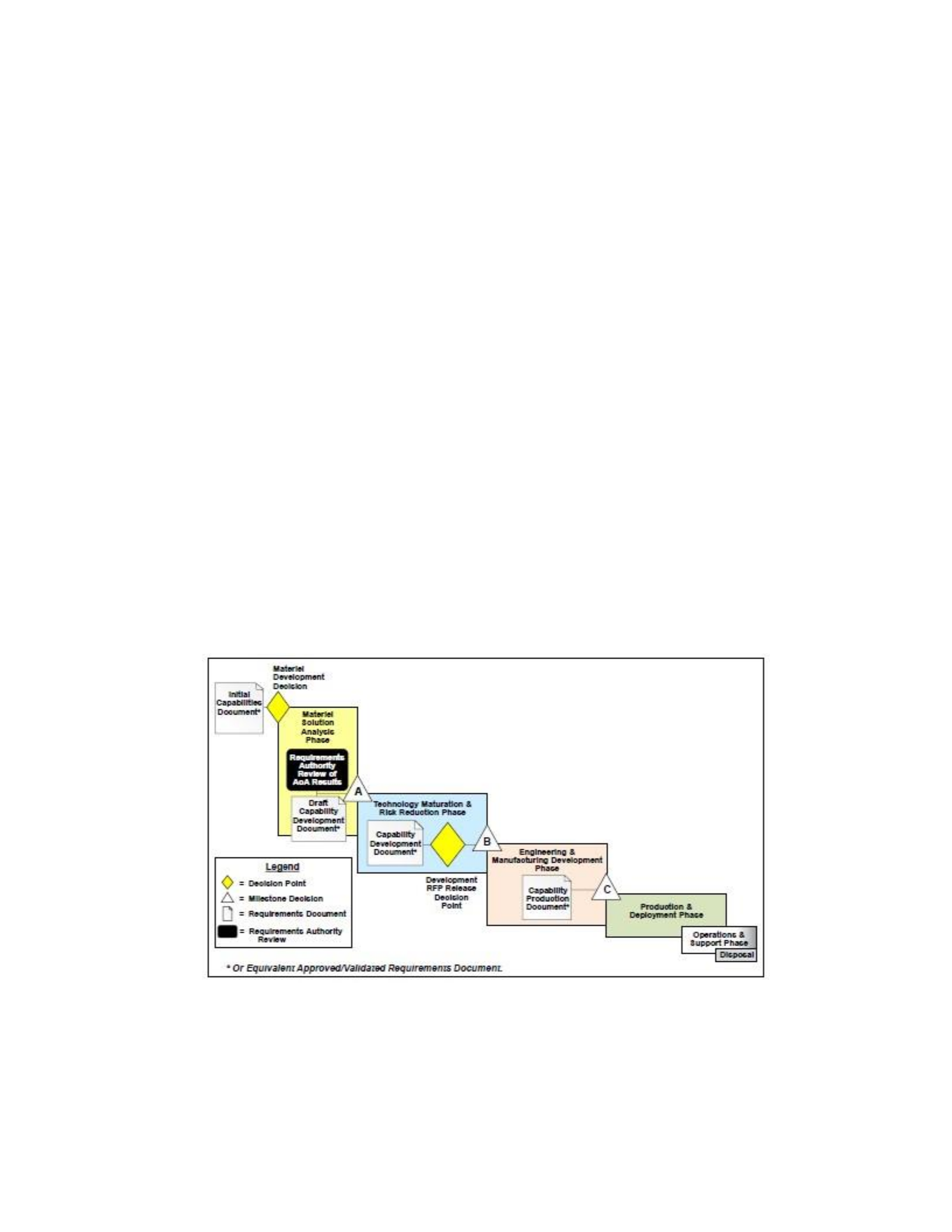
Manual (DoD, Feb 2015). The capability requirements are described in three primary

documents: the Initial Capabilities Document (ICD), Capability Development Document

(CDD), and the Capability Production Document (CPD). The relationship between

capability requirement documents and the acquisition process is shown in Figure 2.

Figure 2: The Relationship between Capability Documents in the Acquisition Process (DoD, 2015: 5)

The ICD contains Measures of Effectiveness (MOEs) that describe mission level

attributes that result in operational effectiveness. The CDD decomposes these MOEs into

task level attributes known as Measures of Performance (MOPs). These MOPs are

primarily described as Key Performance Parameters (KPPs) and Key System Attributes

(KSAs). KSAs are “performance attributes of a system considered critical or essential to

the development of an effective military capability.” (DoD, Feb 2015: D-A-1) KSAs are

“Performance attributes of a system considered important to achieving a balanced

solution/approach to a system, but not critical enough to be designated a KPP.” (DoD,

Feb 2015: D-A-1) Finally, the program can also have Additional Performance Attributes

(APAs), which are not important enough to be KPPs or KSAs but are still important to the

system. MOPs include the description of the attribute and as threshold and objective

parameters for the attribute. The threshold is the lowest value that is operationally

effective or suitable, while the objective value is the desired operational goal. Usually,

performance above the objective value does not justify additional expense. (DoD, Feb

2015) The values between the threshold and objective represents the trade space. Another

important point is that the requirements “are not expected to be static during the product

life cycle. As knowledge and circumstances change, consideration of adjustments or

changes may be requested by acquisition, budgeting, or requirements officials.” (DoD,

2015: 5)

System Requirements Definition

While the capability requirements (and their associated documents) define the

required behaviors of the weapons system, they do not explicitly define the design of the

system. Instead, the capability requirements are used to inform the system requirements,

which generally include performance requirements that are either identical to, or derived

from, the capability requirement KPPs and KSAs. In addition, the program office adds

further requirement attributes to drive “selection of a realistic and affordable solution to the

warfighter’s [capability requirements].” (DoD, 2010: 4) These additional attributes will

include relevant system architecture or interface specification requirements identified through

the systems engineering process. In the words of the OSA Contract Guidebook,

because the System Specification defines the attributes of the overall system to be

developed, this document must describe how the technical system characteristics

will contribute to overall system openness (such as its modularity and how open

standards will be incorporated). (OSA Data Rights Team, 2013: vi)

Additional discussion on architecture requirements will be provided later in this

chapter.

Modular Open System Approach

Acquisitions programs shall be managed through the application of a systems

engineering approach that optimizes total system performance and minimizes

total ownership costs. A modular, open-systems approach shall be employed,

where feasible. (DoD, 2007: 9)

This guidance, found in DoDD 5000.01, represents a major point of emphasis for

the DoD. But what is MOSA?

What is MOSA?

MOSA combines principles of open systems with business strategies for

competitive and affordable acquisition and sustainment of a weapons systems throughout

its lifecycle. MOSA is NOT an open system; rather, it is an approach to develop an open

weapon system that should experience a range of benefits throughout its life. In this

paper, the term MOSA is utilized to refer to the specific DoD initiative, while Open

System Architecture (OSA) is used to refer to a specific implementation that follows a

more generic definition of open architectures. MOSA will likely include OSA and open

standards to achieve these goals, but these are enablers to the primary goals of lower cost

and faster delivery.

MOSA as a specified technique for DoD acquisition traces its roots to 1994, when

the Open Systems Joint Task Force (OSJTF) was chartered. This effort resulted in the

Program Managers Guide: A Modular Open System Approach (MOSA) to Acquisition.

This guide defines MOSA, including the MOSA principles, and provides a variety of

additional tools and guidance that are intended to be useful to program managers. The

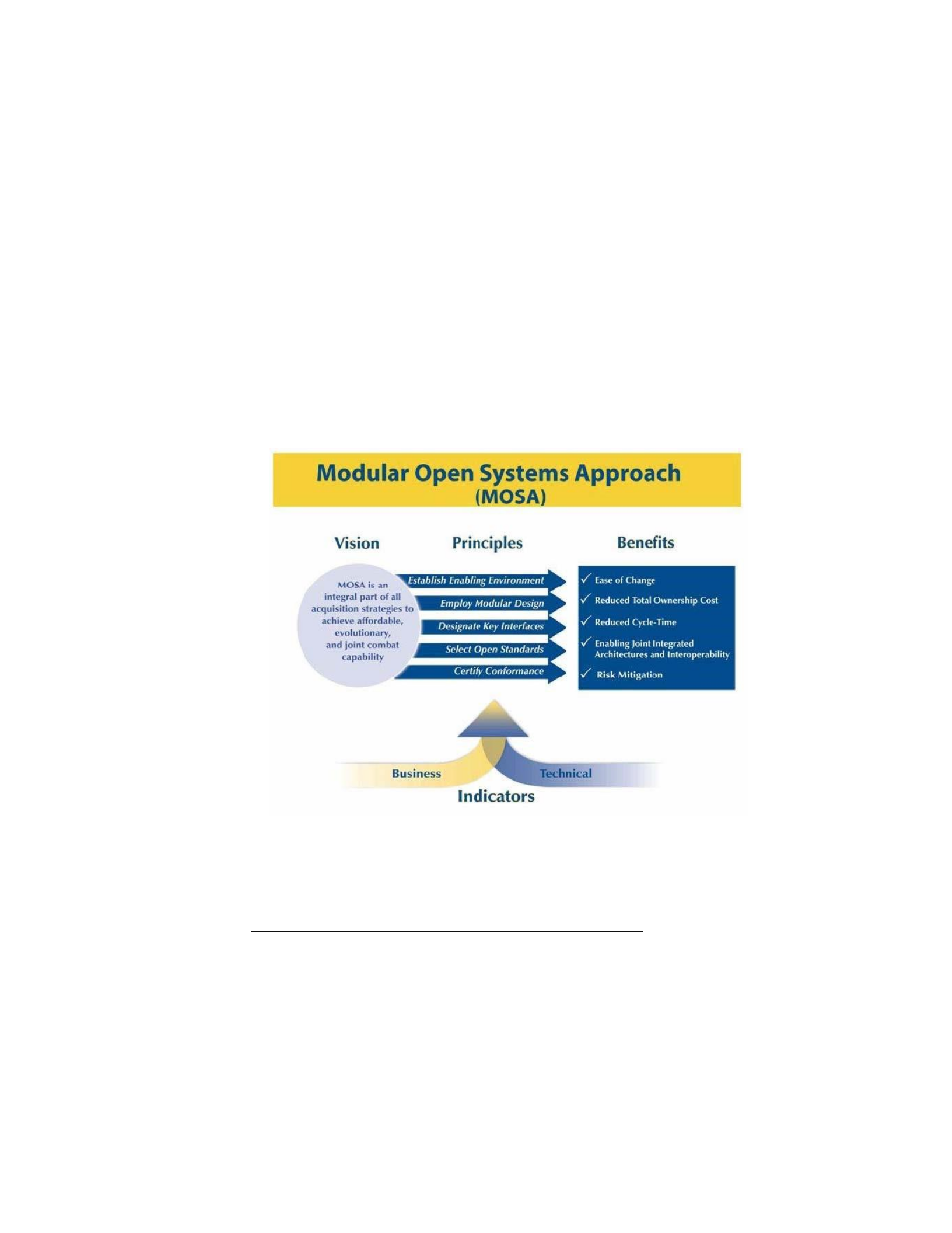
MOSA vision is shown in the figure below (OSJTF, 2004: 3):

Figure 3: Modular Open Systems Approach (OSJTF, 2004: 3) The

OSJTF guide suggests five MOSA principles, discussed below:

MOSA Principle 1: Establish Enabling Environment

In order for MOSA to be successfully applied, the program team must create an

environment that supports the effective development (and sustainment) of open systems.

This encompasses a wide variety of activities, ranging from business practices to support

strategies. The OSJTF outlines practices required for establishing an enabling

environment. (Table 1 (OSJTF, 2004: 11)).

Table 1: MOSA Enabling Environment Supportive Practices

Program and System Level requirements and system level functional performance

specifications.

Configuration management processes that track key interfaces and standards

throughout the life of the program.

Program staff with training or relevant experience in OSA

Assignment of responsibilities for implementing MOSA.

Program management and acquisition planning efforts conducive to MOSA

implementation

Effective identification and mitigation of barriers or obstacles

Application of standard reference models and architectural frameworks

Continuing market research and analysis

MOSA Principle 2: Employ Modular Design

A key aspect of MOSA is the use of modular design. Modular design is

recommended by the OSJTF (MOSA is explicitly Modular), the OSA Guidebook for

PM’s, and throughout the commercial sector. As described by the OSJTF, modularity

principle is “maximal cohesiveness of the functions and minimal coupling among

elements.” (OSJTF, 2004: 13) Fully coupled in this context means that elements are

permanently and uniquely dependent on each other in the performance of an internal

workflow. Modularity is a description of system partitioning that results in:

• Modules that are scalable, reusable by other modules within a system

and/or by other systems, and consist of isolated, self-contained functional

units

• Disciplined definition of interfaces between modules, that are usually open

and published interfaces

Modular designs, by definition, permit substitution of units with similar

components or products from alternate sources with minimum impact on existing units.

Modularity is a highly desirable attribute; a highly modular system will support the

ability of acquiring, modifying or repairing smaller (and usually cheaper) components

independently rather than as a larger system. On the other hand, tightly coupled processes

are very efficient for their singular purpose. Balancing the efficiency of tight coupling

with the flexibility of modular systems is part of the optimization inherent in the system

engineering process.

The number and variety of interchangeable modules, and the ease with which they

can be interchanged, determines how open the system is. Additional measures of

openness can include the time and cost required to change a module, or the number of

independently provisioned modules. Conceptually, the way to go about designing a

modular and open system is to first study critical work/mission threads associated with

the system domain. Then, perform market analysis of relevant existing OTS components,

and optimize a system by assembling the components. Finally, the program office must

plan to close requirement gaps by either incremental improvement to existing modules

and/or developing new modules. Figure 4 shows a generic example of a modular design.

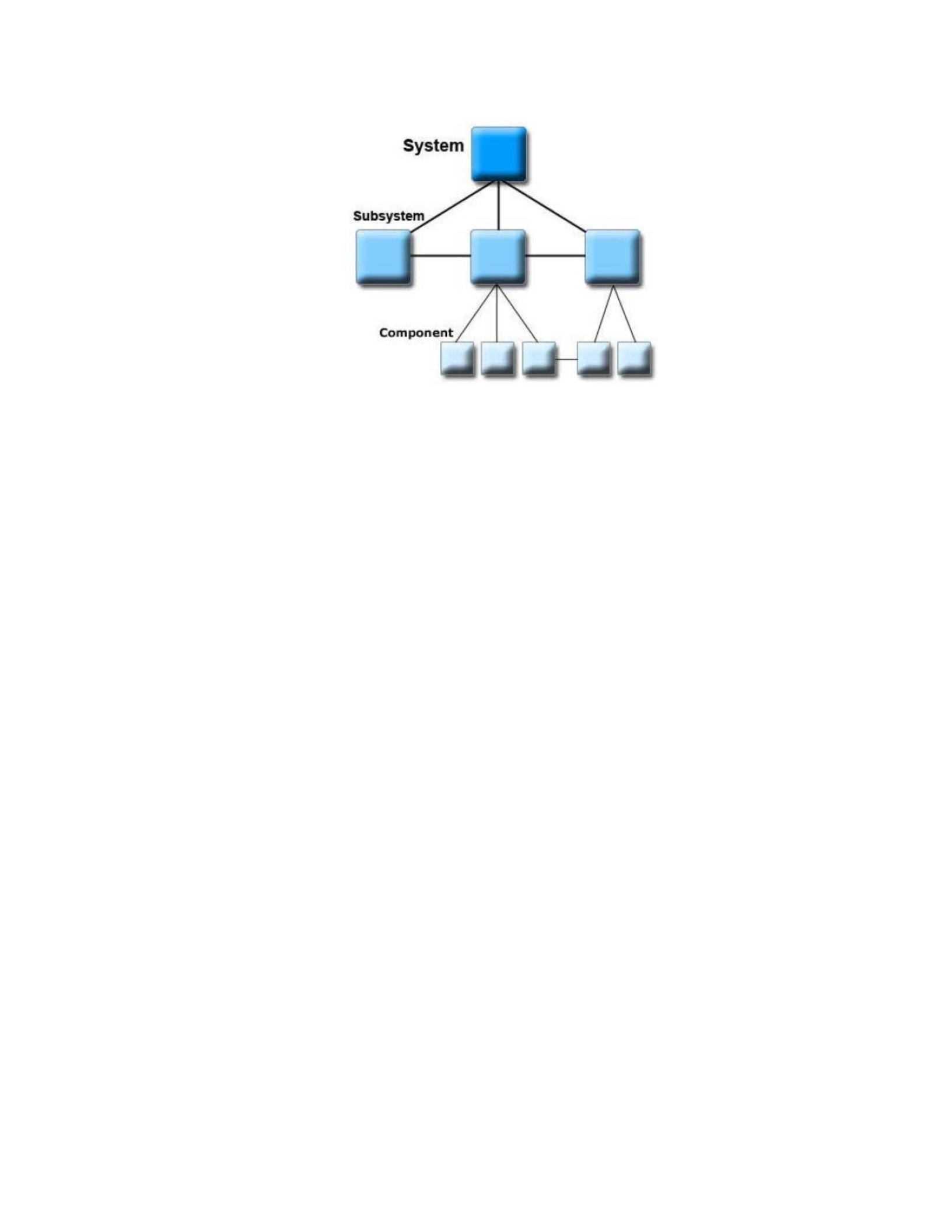
Figure 4: Decomposition of a System into its Modular Design (DAU, 2015)

The information technology sector provides additional guidance and tools for

developing modular designs. The commercial sector tends to align modular information

systems into what it calls “product lines.” The Carnegie Mellon Software Engineering

Institute (SEI) is among the pioneers of software product lines. SEI has provisioned a

suite of engineering level training materials and tools to assign developers in designing

modular systems. (SEI, 2017) Another commercial concept for modular design is the

Service Oriented Architecture (SOA) paradigm. “Service Oriented Architecture is a

paradigm for organizing and utilizing distributed capabilities that may be under the

control of different ownership domains.” (Federal CIO Council, 2008: vi) There are a

wide variety of tools for developing SOA, including the Practical Guide for Federal SOA,

which was compiled as a government-industry collaboration. (Federal CIO Council,

2008). The Model Driven Architecture (MDA) is another suite of tools and practices

maintained by the Object Management Group (OMG) for aligning concepts like MOSA

and SOA with intended mission and business outcomes. (OMG, 2017) These tools,

among others, are highly useful to programs as they work to develop modular and open

systems.

MOSA Principle 3: Designate Key Interfaces

The OSJTF defines an interface as “the functional and physical characteristics

required to exist at a common boundary or intersection between systems or items.”

(OSJTF, 2004: A2) Interfaces can be software (messaging, streaming data, etc…),

hardware (Ethernet cables, computer chassis, etc…), electrical (28VDC power), etc…

Use of modular design requires careful treatment of multiple levels of interfaces. The

choice of modules will in many cases drive the options for and selection of modules. In

other cases, the choice of interface will constrain the selection of modules. It should be

noted that existence of an interface does not in and of itself imply the existence of a

module in the context of MOSA. Note that the OSJTF definition of interface does not

explicitly call out modules; as a result, systems and/or items connected by interfaces are

not necessarily modules as defined above. For example, multiple closely coupled

software components can communicate with each other using open standard operating

system messages. These components do not constitute a modular design, because the

software components are not self-contained; remove one and the other fails.

Some system interfaces are particularly important because they “transmit critical

data, information, materiel or services.” (OSJTF, 2004: A2) They may also be of high

interest because they represent areas of “rapid technical change, a high rate of failure, or

costliness of connected modules.” (OSJTF, 2004: A2) DAU calls these interfaces “key

interfaces,” explaining that they represent areas where openness is strongly preferred. In

the MOSA context, interfaces that allow the decoupling necessary to incorporate critical

modularity are intended to be key. A generic diagram showing the various types of

interfaces is shown in Figure 5, which expands on Figure 4.

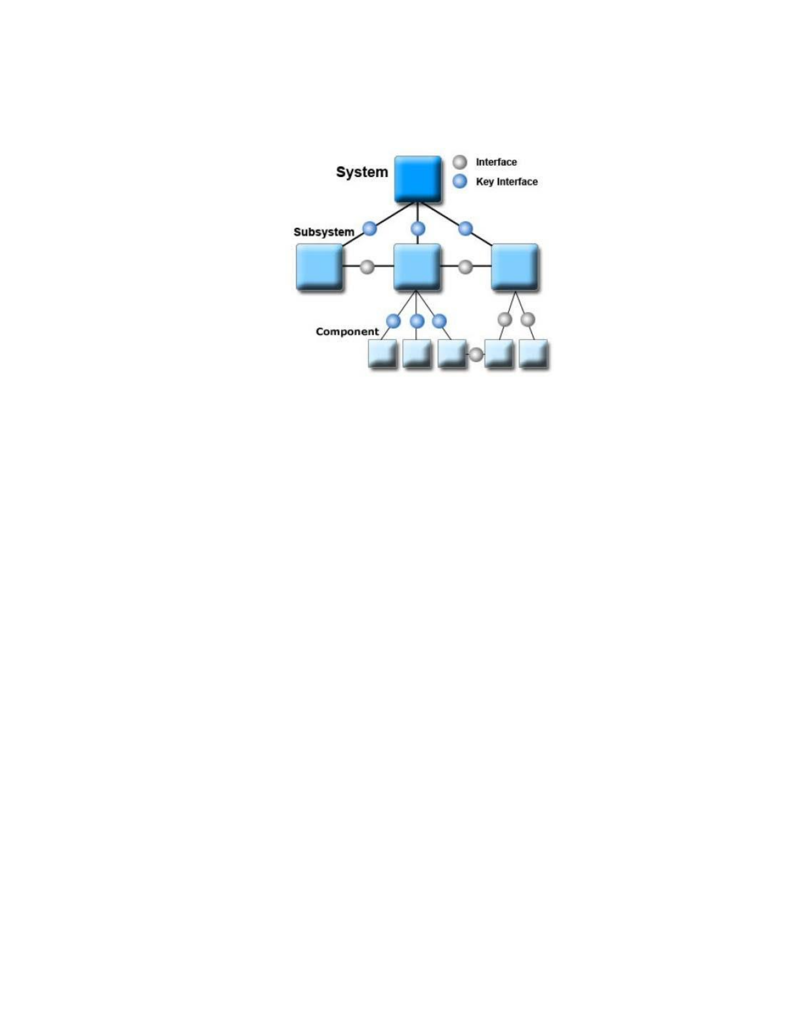
Figure 5: Decomposition of a System Showing Multiple Interface Types (DAU, 2015)

The OSJTF MOSA guidance states that “programs must determine the level of

implementation (e.g., subsystem, system, system-of-systems) at and above which they

aspire to maintain control.” (OSJTF, 2004: 14) The OSTJF assumes that “control”

requires unlimited intellectual property rights, and that the need to control interfaces

breaks neatly at the boundary between components as shown in Figure 5. However, more

recent DoD experience and guidance provides a more nuanced view of data rights. An

example of this is the guidance for “Owning the Technical Baseline,” given by the Air

Force Lifecycle Management Center. (Imlay, 2016) OTB mandates careful analysis of

the level of intellectual property rights necessary to achieve government objectives. For

example, the government may need to acquire detailed low level data defining

aircraftweapons interface. In contrast, the government may not need to acquire source

code for a major enterprise operating system (such as Microsoft Windows). According

to the OSJTF,

defining the level of interface control too low may limit efficient technology

insertion, while defining the level too high may lead to the use of proprietary

interfaces for major system components resulting in limited supplier support.

(OSJTF, 2004: 14)

Phrased a different way, not acquiring sufficient data rights (defining the level too

high) may result in vendor lock, while insisting on too many data rights (defining the

level too high) may preclude access to the best commercial solutions. These twin risks

make the OTB analysis of required intellectual property rights one of the most important

activities for a program employing MOSA.

MOSA Principle 4: Select Open Standards

Once key interfaces are identified, the program team select standards for key

interfaces. According to the OSJTF key interfaces are strongly desired to be open,

(OSJTF, 2004: 14) but there is significant flexibility provided to the program to make

decisions about the implementation of interfaces to meet program risk management

objectives. The OSJTF and DAU frame the standard selection in the context of multiple

types of standards that can be utilized for each interfaces. They define these types based

on two primary criteria: market acceptance, and degree of openness. Market acceptance

reflects how widely the standards are used within the commercial market. Widely

accepted standards offer the maximum possibility for a program to select solutions that

natively conform to the standard, whereas narrowly accepted standards are more likely to

require modification of the solution. The DAU describes the degree of openness by how

much information is freely available about the standard. The spectrum of standard types

defined by DAU are shown in Figure 6, while Figure 7 extends the previous DAU

provided system diagram to include standard interfaces.

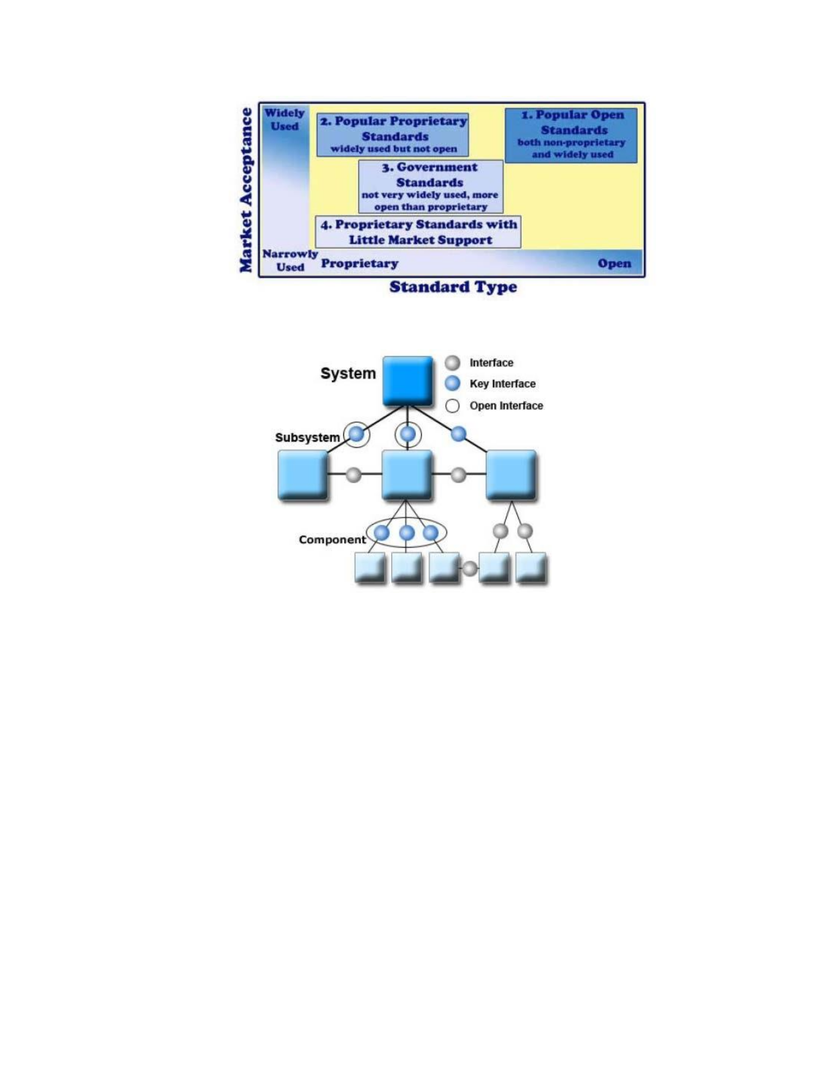
Figure 6: Types of Standards as related to Openness and Market Acceptance (DAU, 2015)

Figure 7: Decomposition of a System showing Open Interfaces (DAU, 2015)

There are many other definition of openness. In particular, consider the World

Wide Web Consortium’s (W3C) requirements for an open standard (W3C, 2017):

• transparency (due process is public, and all technical discussions, meeting

minutes, are archived and referencable in decision making)

• relevance (new standardization is started upon due analysis of the market

needs, including requirements phase, e.g. accessibility, multi-linguism)

• openness (anybody can participate, and everybody does: industry,

individual, public, government bodies, academia, on a worldwide scale)

• impartiality and consensus (guaranteed fairness by the process and the

neutral hosting of the W3C organization, with equal weight for each

participant)

• availability (free access to the standard text, both during development, at

final stage, and for translations, and assurance that core Web and Internet

technologies can be implemented Royalty-Free)

• maintenance (ongoing process for testing, errata, revision, permanent

access, validation, etc.)

The W3C definition is particularly useful because it is broad in scope, and also

provides reasonably objective, observable criteria across the scope of the definition.

The OSJTF further states that key interfaces should be “examined very carefully

to insure that the use of an open standard is both feasible and appropriate based on

performance and business objectives.” (OSJTF, 2004: 16) It is interesting that this

guidance by the OSJTF is not further developed within the MOSA literature. The concept

of open versus closed is meant to be an indicator of the program’s ability to meet the

objectives of MOSA. For example, under the W3C definition, it is plain to see why more

open interfaces tend to lead to modules that are replaced/modified faster and cheaper.

Conversely, interfaces that are not commonly used or have restricted data rights (i.e.

closed) tend to take longer and are more costly to replace or modify. The formal

definition of “proprietary” conveys that the owner has exclusive rights to control use and

access. In that sense, many proprietary standards, e.g. the ones owned by standards

bodies, are also open. However, in government-facing MOSA literature, “proprietary”

implies that access and use is relatively restricted. These messy semantics are

exacerbated by the fact that open and closed do not have universal precise engineering

definitions. Aids such as Figure 6 and Figure 7 are meant by DAU to assist programs in

selecting interface standards, but only provide additional heuristic guidance rather than

prediction of MOSA outcomes. The selection of modules and interfaces is dependent on

the functional design that arises from business case analysis together with market analysis

of potential modular components (current and future) and their associated interfaces. This

process should include analysis of multiple interface standards, and how each one will

enable the program’s business objectives. This should be accomplished by focusing on

targeted measurable outcomes rather than on characterizing a particular module or

interface as “open” or “closed.”

MOSA Principle 5: Certify Conformance

The true value of conformance to any particular standard in an open system is

whether the artifact of interest actually contributes to specified measures of performance

and/or effectiveness. There are a continuum of strategies for verifying and validating

conformance. Within the context of MOSA, verifying conformance refers to assuring

compliance with the standard, while validating refers to assuring that the standard

achieves the desired outcomes. In this sense, validation necessarily extends beyond

testing of standard compliance to include functional and/or performance testing at the

system or system of systems level. Some approaches trust the vendors internal testing.

Other approaches include verification and validation testing performed by an organization

external to the program. A detailed discussion of conformance inspection is outside the

scope of this document, and is not required for the analysis described in Chapter III.

MOSA Evaluation Tools

The development of a system using MOSA is a complicated endeavor; as proven

by the many unsuccessful programs within the DoD. To assist programs acquiring a

MOSA system, a variety of tools have been created. These range from guidebook, to

design tools, to evaluation software. This section provides a limited overview of extent

tools.

Open Systems Architecture Contract Guidebook for Program Managers

The DoD Open Systems Architecture Contract Guidebook for Program Managers

(OSA Data Rights Team, 2013) was written to assist programs developing systems using

open architectures. This extensive document identifies specific guidance for PM’s in

terms of how they implement MOSA into systems acquisition contracts. The guidebook

provides robust contract language that can be tailored to a program’s needs, including

Statement of Work, Evaluation Criteria, Contract Data Requirements Lists. However, this

guidance stops short of providing specific technical details for implementation of MOSA

on a program. For example, the guidebook does not list specific standards that would be

implemented or provide common definitions of key interfaces. Rather, it provides tools

and best practices for a program office to use once it has made these architectural

decisions. Phrased a different way, the guidebook pre-supposes that the program has

already completed an analysis of alternatives and developed a business case for the

program.

Open Architecture Assessment Tool

Another tool developed to support open architecture acquisition is the Open

Architecture Assessment Tool (OAAT). (Naval OA Enterprise Team, July 2009) This tool,

developed by the US Navy, is intended to assess programs to determine their level of

openness through a questionnaire that evaluates the program in programmatic and

technical areas. Each area is assessed by a series of questions that are answered

subjectively by the program team. The programmatic area contains 41 messages that

discuss a variety of concerns, including:

• Minimization of modifications to open standards that limit flexibility

• Scope of unique development

• Limitation of impact of proprietary solutions on openness

• Requirements compliance with JCIDS

• Requirements compliance with Interoperability and Supportability

references

• Spiral development

• Exportation of reusables, flexibility/openness

• Prime System Integrator competitive assignment

The technical areas include 30 questions, spread among the following topics:

• Interoperability (6 questions): How readily can the program’s separate

systems exchange information and appropriately utilize each other’s

functional capabilities?

• Maintainability (2): What architectural characteristics address

obsolescence and provide for timely technology refresh, fixes, and

upgrades?

• Extensibility (3): Does the program follow a well-defined System

Engineering process for implementing capability extension?

• Composability (2): Are the program’s systems capable of being highly

modular and having minimal dependencies (loosely coupled) so they can

be readily combined with other modules to provide new types of

functionality?

• Reusability (4): Are the assemblies that are candidates for reuse readily

available, certified for reliability and performance, and easily obtained for

reuse?

• General Design Tenet (13): General design questions related to MOSA

applications

After the questionnaire is completed, the results are tabulated, mathematically

combined, and graphically displayed on a chart based on the Open Architecture

Assessment Model (OAAM)(Figure 8). This chart allows programs to be compared

visually based on their expected level of openness.

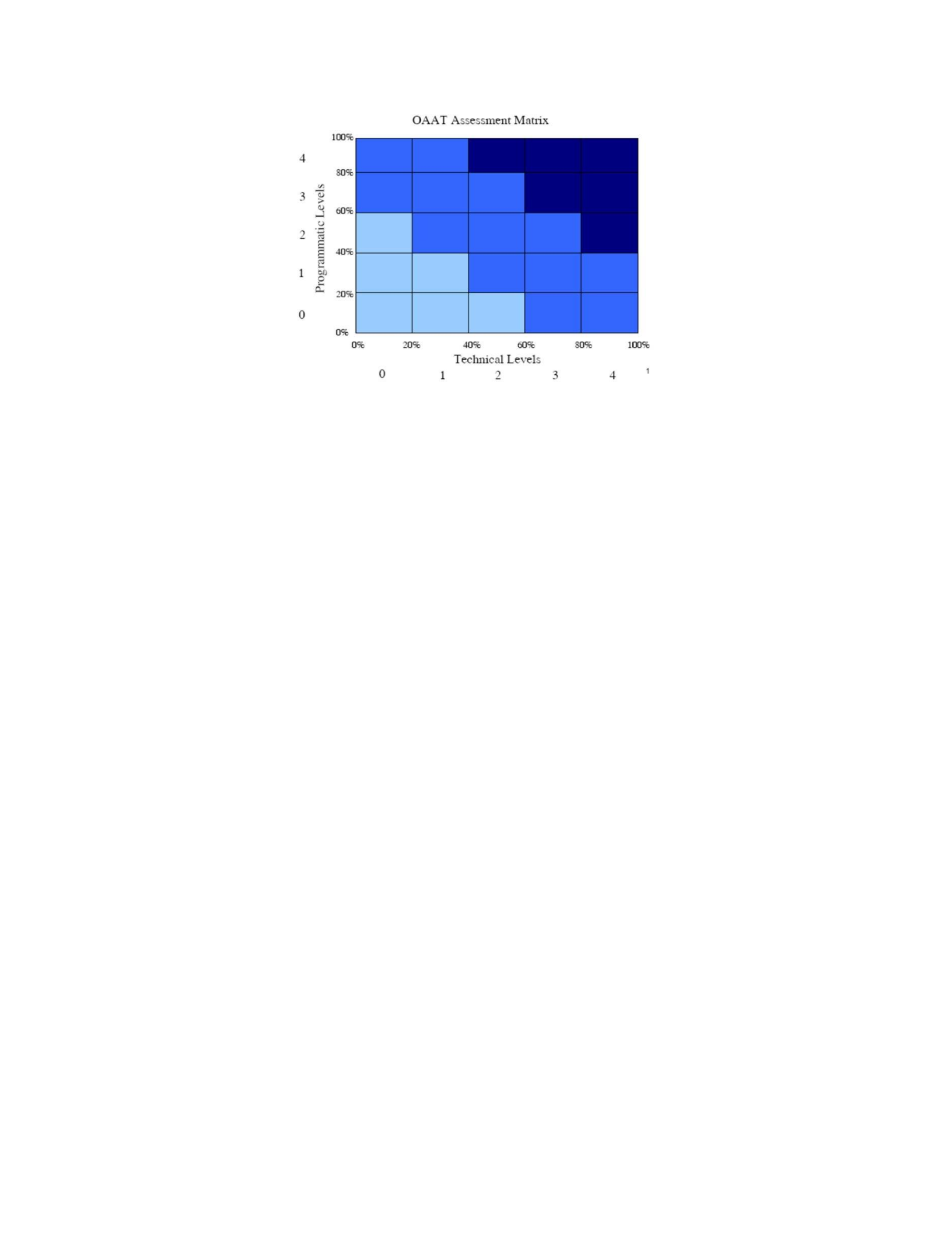
Figure 8: Open Architecture Assessment Matrix Resulting from OAAM Analysis (Naval OA

Enterprise Team, July 2009)

This tool has been utilized by weapon system programs, but also by several US

Navy research efforts.

While OAAT is effective for evaluating programs across an enterprise, it provides

little utility for a single program evaluating multiple architecture alternatives. The

business areas provide little discrimination between approaches because they would

likely be applied across all alternatives a single program would consider. The technical

areas have potential to be effective, but the subjective choices have limited granularity.

The following are examples of questions (Naval OA Enterprise Team, 2009):

• “To what extent are open standards selected for key interfaces?” The

available answers are: “N/A, None, Little Extent, Moderate Extent, Large

Extent.”

• “To what extent can system components be substituted with similar

components from a competitive source?” The available answers are: “N/A,

None, Little Extent, Moderate Extent, Large Extent.”

• “To what extent do the system level functional and performance

specifications permit an open system design? The available answers are:

“N/A, None, Little Extent, Moderate Extent, Large Extent.”

The OAAT provides is no quantification of the answers and no consideration for

how each selection impacts the end result of lower cost or faster delivery. For example,

the program may use 50% open interfaces. Is this low, moderate or high? If the 50%

covers all potential modifications, it may actually support the business objectives of the

program even though the analyst may not consider the approach to have a large extent of

open interfaces. It is also likely that multiple alternatives would score similarly well. If

only one interface changes, does it change the answer from large to moderate? This lack

of granularity makes the OAAT ineffective at estimating the cost effectiveness of

different architectural approaches.

Key Open Sub System Tool

Another US Navy developed open architecture tool is the Key Open Sub System

(KOSS) tool. KOSS was developed in 2008 by the Naval Open Architecture Enterprise

Team to assist programs complying with Principle 3 of MOSA, enabling them to identify

“volatile Subsystems/Components that would yield the greatest benefit to lifecycle

affordability by applying MOSA principles.” (Naval OA Enterprise Team, 2009: 4) KOSS

enables programs to evaluate the effect of different design choices. The program team

decomposes the system into system components in four categories: hardware, software,

middleware and operating system. Once this is done, the team creates a capability map,

which determines when components are expected to change, and a rate of obsolescence.

Additionally, the team determines a relative cost of change and relative weapon system

capability improvement. Using the rate of obsolescence and the capability map, KOSS

determines a relative rate of change for each component. Using the relative rate of change

and relative cost of change, the KOSS tool calculates an open architecture applicability

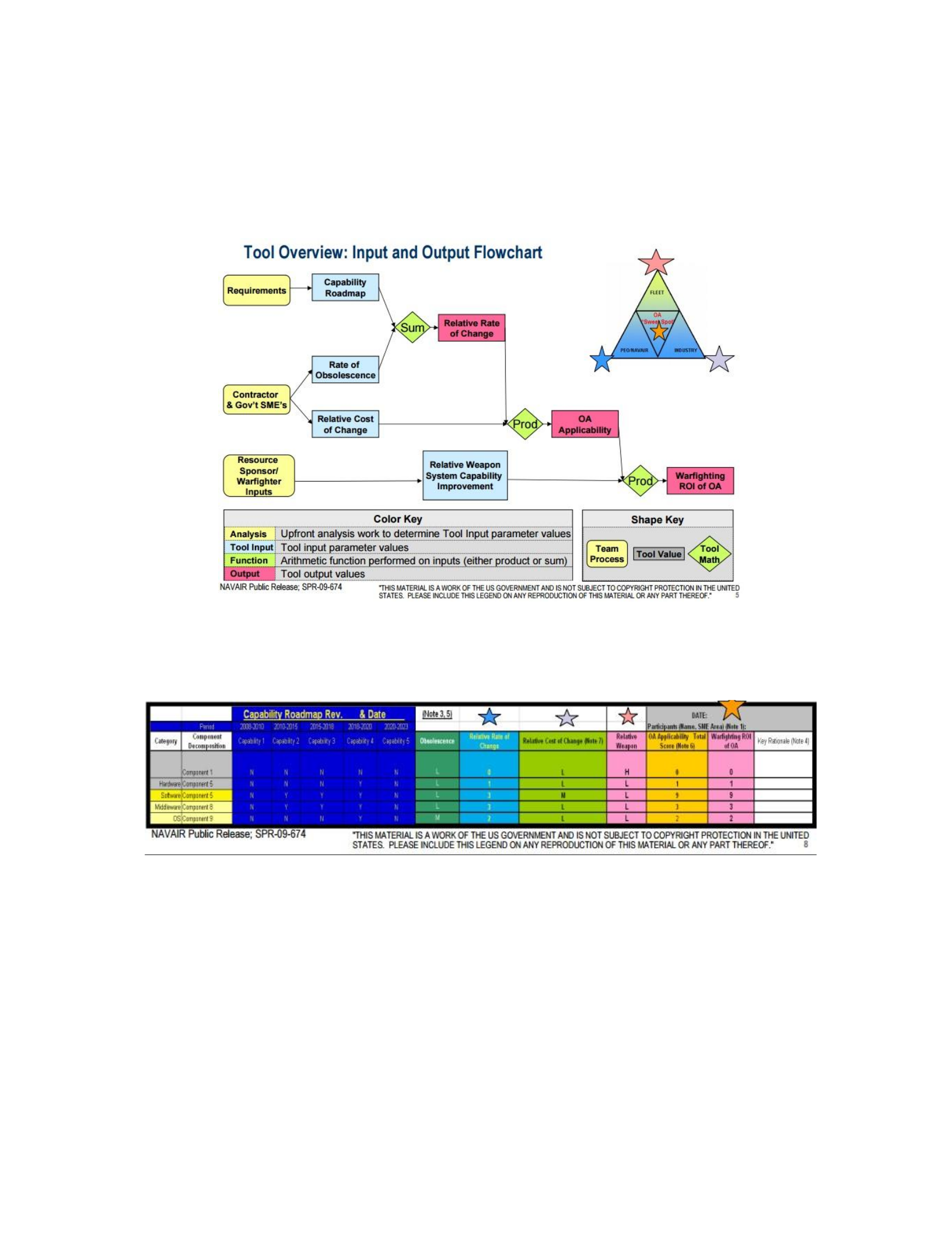
score. Using the open architecture applicability score and the relative weapon system

capability improvement score, the KOSS tool calculates a warfighter return on

investment. This process is shown pictorially in Figure 9:

Figure 9: KOSS Tool Overview (Naval OA Enterprise Team, August 2009: 5)

Figure 10: KOSS Tool Example (Naval OA Enterprise Team, August 2009: 8)

The KOSS tool provides a useful service by allowing programs to evaluate

different functional decompositions to understand which system components will need to

be refreshed often, and which are expected to be worth replacing based on the warfighter

ROI. The tool supports qualitative analysis of changes to the system design, as well as

cost, schedule and performance effects. However, the level of technical detail provided by

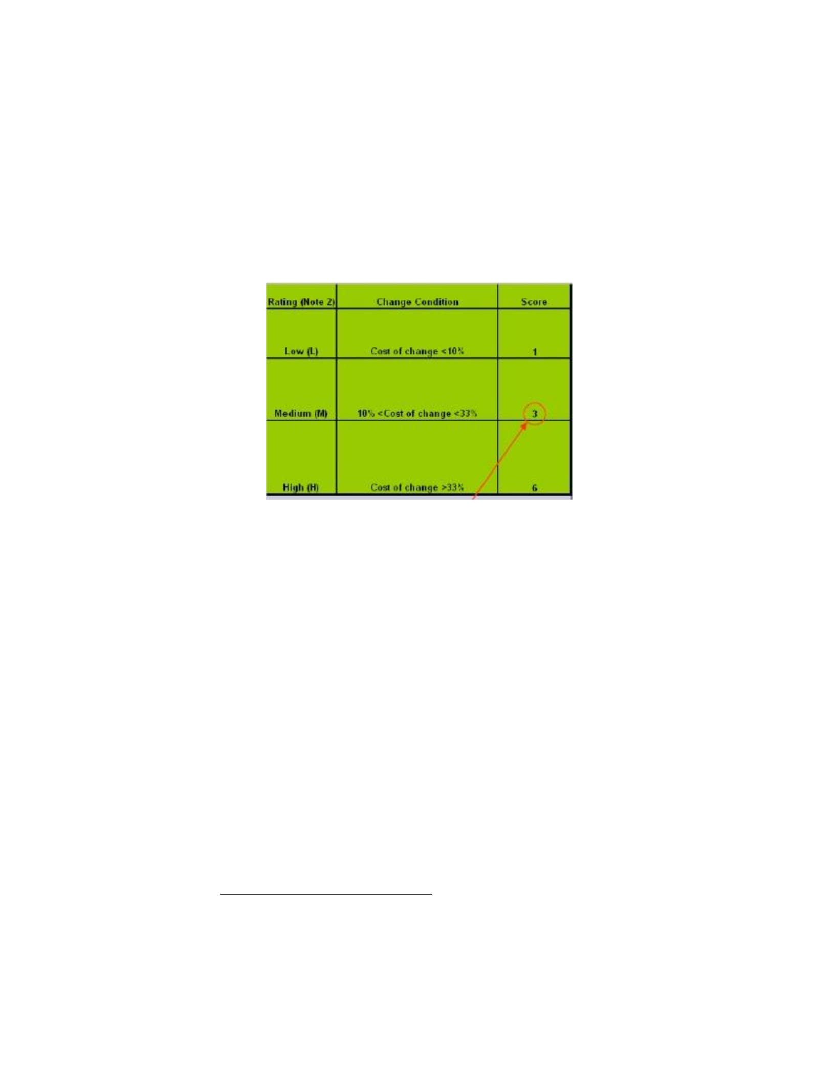
KOSS is limited at best. For example, instead of directly calculating cost, the effect of

cost is accounted for by a “qualitative measure of the cost of changes compared to the

original cost of the component.” (Naval OA Enterprise Team, August 2009: 6) This is

shown in Figure 11.

Figure 11: KOSS Cost of Change (Naval OA Enterprise Team, August 2009: 13)

To create this value, a subject matter expert determines the relative cost change,

which equates to both a qualitative measure and a relative score. The score is then used

for other calculations within the KOSS tool. The course grained qualitative approach

obscures the effect of specific changes within the system. Additionally, the KOSS tool

does not account for the effect of the interfaces between the components. While the

KOSS tool is not particularly useful for evaluating candidate design alternatives, it can be

very useful for a program for identifying which components will need to be replaced at a

higher rate. Other approaches would be required to address the cost effectiveness of

specific alternatives.

Evolutionary Acquisition Model

Another interesting area of research is the Evolutionary Acquisition model (Ford

and Dillard, 2008), which uses control theory to model the dynamic behavior of the

Defense Acquisition System for a given program. Originally designed to model

evolutionary acquisition processes, Ford and Dillard expanded their model in 2008 to

include the effects of open architectures on the system acquisition process (Ford and

Dillard, 2008). In 2009 they performed a case study using the US Navy’s Acoustic Rapid

Capability Insertion (ARCI) program (Ford and Dillard, 2009). Their research

mathematically demonstrated that evolutionary approaches and open architectures can be

combined to deliver capability to the warfighter faster and cheaper. While useful research,

the model proposed by Ford and Dillard focused on modeling the behavior of the

evolutionary programmatic approach and not modeling the technical design of the

system.

When applied to development projects, system dynamics focuses on how

performance evolves in response to interactions among development strategy

(e.g., Evolutionary Acquisition versus traditional acquisition), managerial

decision-making (e.g., the allocation of resources), and development processes

(e.g., concurrence).” (Ford and Dillard, 2009: 213)

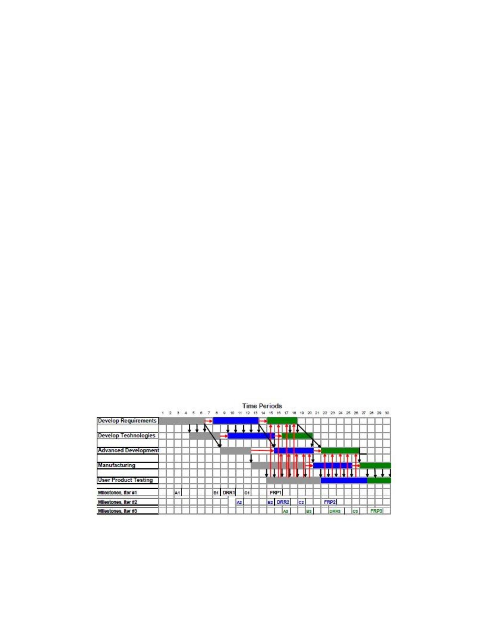
These performance impacts are evaluated within the context of a program

lifecycle. Figure 12 shows a notional evolutionary lifecycle with 3 phases.

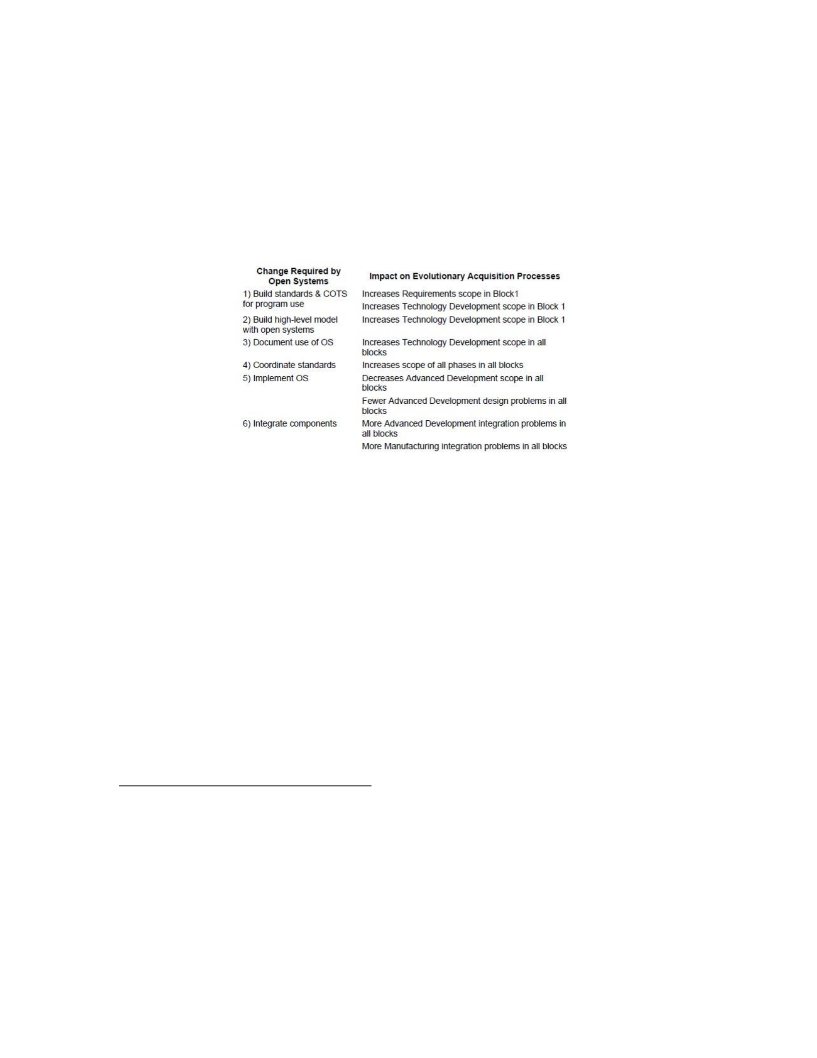
Figure 12: Evolutionary Acquisition Model with 3 Phases (Ford and Dillard, 2008: 14)

Instead of using detailed technical parameters, the authors modeled the effect of

open architectures in relation to their previously developed evolutionary acquisition

model. Table 2 shows these some of these effects.

Table 2: Open Architecture Effects on Evolutionary Acquisition (Ford and Dillard, 2008: 17)

This approach is useful for investigating the use of evolutionary approaches for a

system, but has limited ability to model the technical differences between architecture

alternatives. The effects shown in Table 2 are high level programmatic changes rather

than detailed technical effects. It would be challenging to relate the key interface

definition choices, or the selection of specific standards, to the effects chosen by Ford and

Dillard’s model. Additionally, their model does not take into account the effect to

delivered warfighter capability or the cost of implementing open. Consequently, other

methods would be required to evaluate the cost effectiveness of architecture alternatives.

Architecture Tradeoff Analysis Method

Another analysis model is the Software Engineering Institute’s (SEI) trademarked

“Architecture Tradeoff Analysis Method,” or ATAM, which is designed to facilitate the

analysis of software architecture approaches. In SEI’s words: “Having a structured

method helps ensure that the right questions regarding an architecture will be asked early,

during the requirements and design stages when discovered problems can be solved

cheaply.” (Kazman et al, 1999: 1) SEI developed an approach that utilizes quality

attribute goals to establish levels of utility for architecture approaches. The ATAM uses

the following process (SEI, 2016):

1. Present the ATAM. The evaluation leader describes the evaluation method

to the assembled participants, tries to set their expectations, and answers

questions they may have.

2. Present business drivers. A project spokesperson (ideally the project

manager or system customer) describes what business goals are

motivating the development effort and hence what will be the primary

architectural drivers (e.g., high availability or time to market or high

security).

3. Present architecture. The architect will describe the architecture, focusing

on how it addresses the business drivers.

4. Identify architectural approaches. Architectural approaches are identified

by the architect, but are not analyzed.

5. Generate quality attribute utility tree. The quality factors that comprise

system "utility" (performance, availability, security, modifiability,

usability, etc.) are elicited, specified down to the level of scenarios,

annotated with stimuli and responses, and prioritized.

6. Analyze architectural approaches. Based on the high-priority factors

identified in Step 5, the architectural approaches that address those factors

are elicited and analyzed (for example, an architectural approach aimed at

meeting performance goals will be subjected to a performance analysis).

During this step, architectural risks, sensitivity points, and tradeoff points

are identified.

7. Brainstorm and prioritize scenarios. A larger set of scenarios is elicited

from the entire group of stakeholders. This set of scenarios is prioritized

via a voting process involving the entire stakeholder group.

8. Analyze architectural approaches. This step reiterates the activities of Step

6, but using the highly ranked scenarios from Step 7. Those scenarios are

considered to be test cases to confirm the analysis performed thus far. This

analysis may uncover additional architectural approaches, risks, sensitivity

points, and tradeoff points, which are then documented.

9. Present results. Based on the information collected in the ATAM

(approaches, scenarios, attribute-specific questions, the utility tree, risks,

non-risks, sensitivity points, tradeoffs), the ATAM team presents the

findings to the assembled stakeholders.

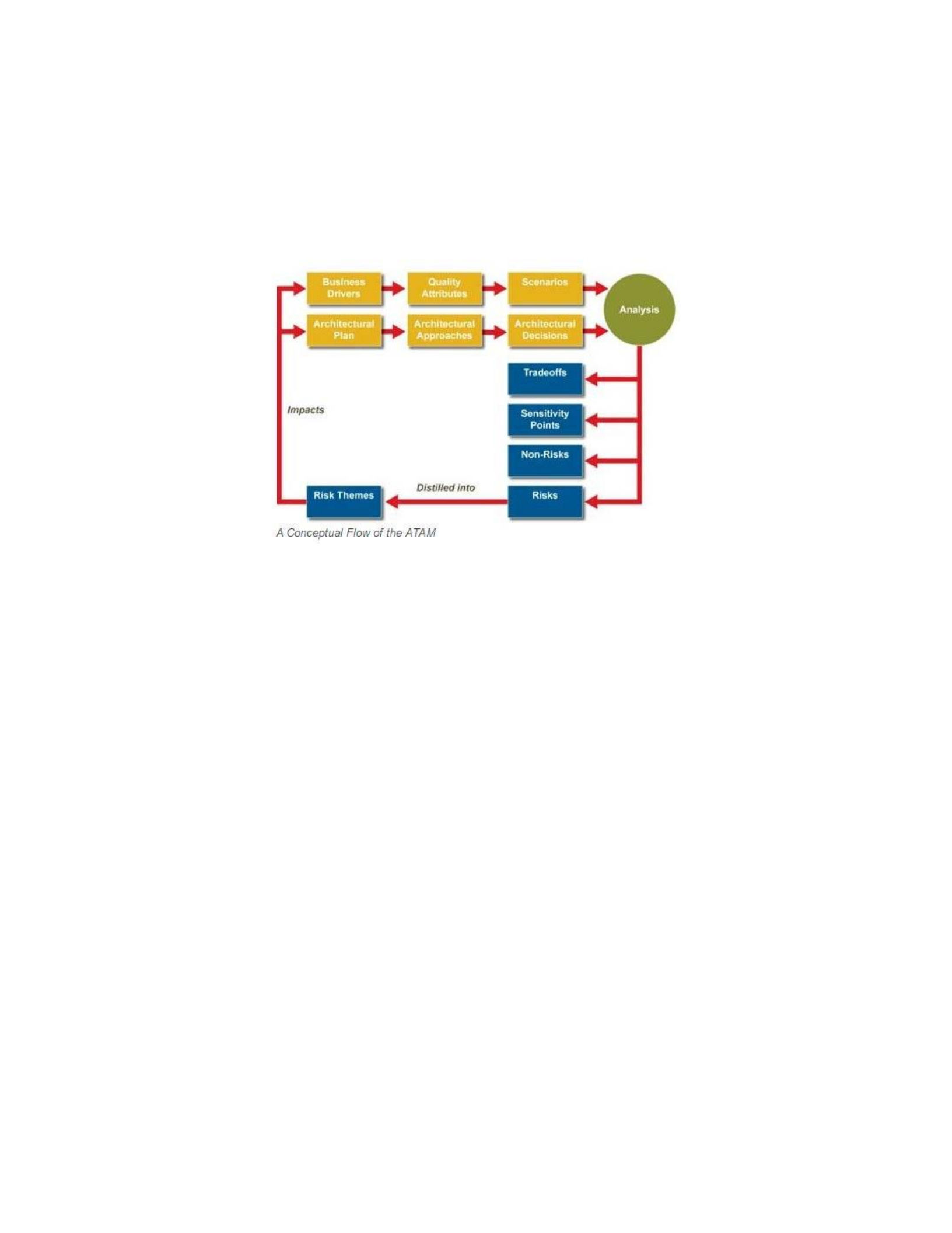
The conceptual flow of ATAM is shown in Figure 13.

Figure 13: Architecture Tradeoff Analysis Method Conceptual Flow (SEI, 2016)

The ATAM is purpose-built to compare the quality of the software architecture

approaches by using an attribute tree to measure the quality of the delivered software in

relation to the system’s architecture choices. Quality attributes are determined based on

the business drivers; for example the availability of the system, or its latency under a

specific scenario. Evaluating these attributes using a quality hierarchy allows the analyst

to evaluate disparate architecture approaches to determine the best path forward.

Overall, the ATAM is a very useful tool for estimating the quality of software

delivered based on the architecture decisions made by the program. It provides a useful

framework for logically working through the decision space, and allows for iterative

analysis to refine the design. However, the ATAM has several important limitations. (1) It

does not evaluate cost separate from other attributes, (2) It does not evaluate the

performance of the system over its lifecycle, and (3) It does not evaluate the effect of

modifying the system with new components throughout the lifecycle. Consequently,

while the Attribute Hierarchy and related business goals are highly useful, a different

framework is necessary for evaluating cost effectiveness.

Reference Architectures

Reference Architectures, while not a strictly MOSA tool, are effective aids for

employing open designs. According to the DoD Office of the Chief Information Officer,

the DoD definition for Reference Architecture is “an authoritative source of information

about a specific subject area that guides and constrains the instantiations of multiple

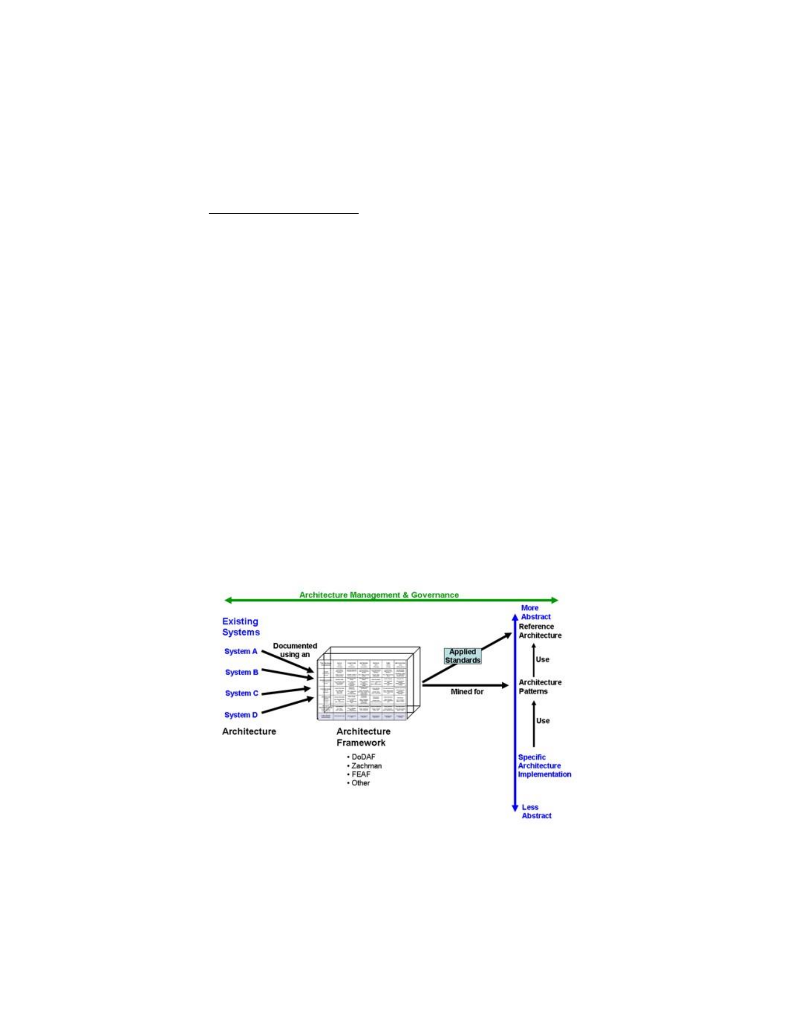
architectures and solutions.” (DoD, June 2010: 3) In contrast, a system architecture is an

instantiation where “the generalized and logical abstract elements of the Reference

Architecture are replaced by real world, physical elements according to the specified

rules, principles, standards and specifications.” (DoD, June 2010: 3) This is shown

pictorially in Figure 14, along with the relationship to the architecture framework that

documents the system architecture.

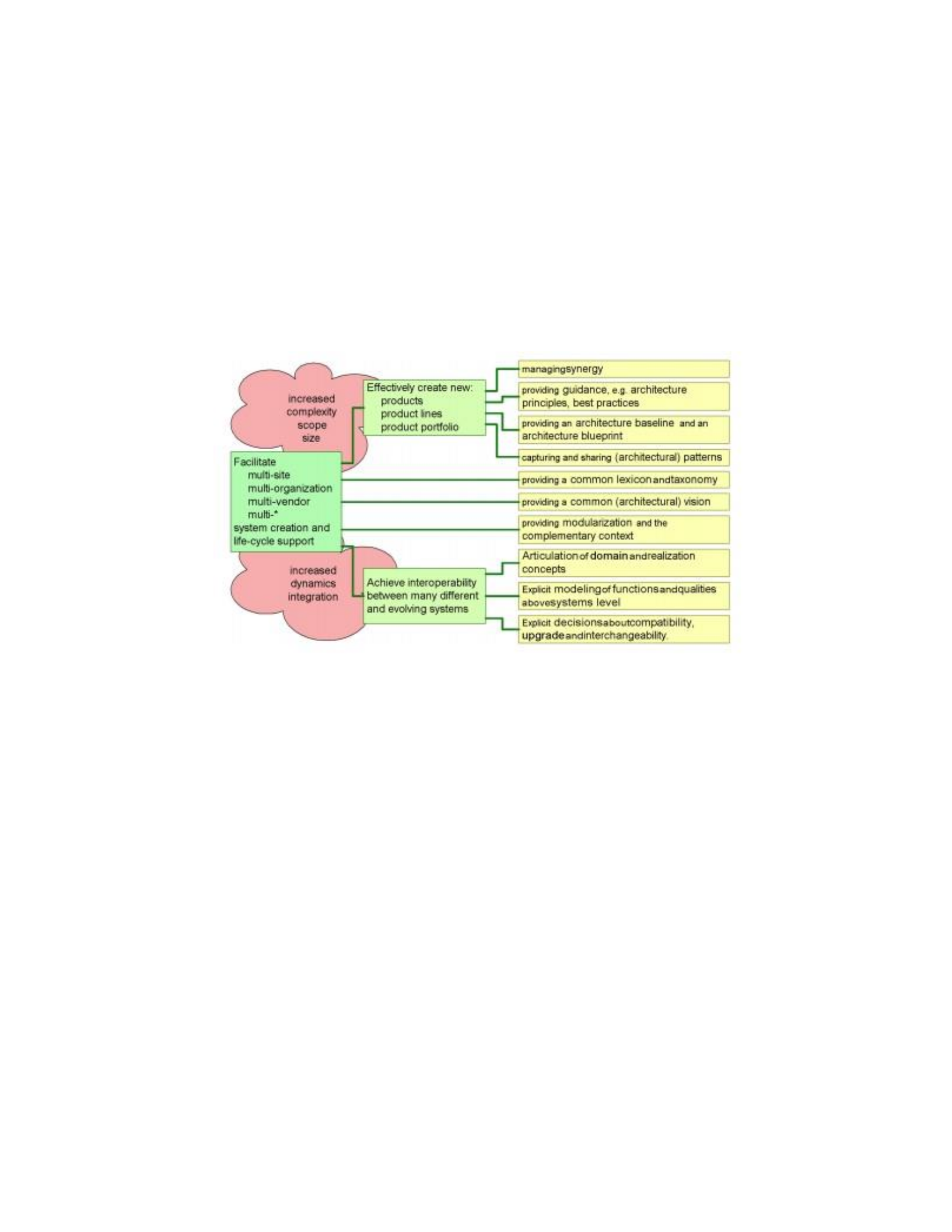
Figure 14: Architecture Management Relationships (Cloutier, et al 2008)

While the concept of Reference Architectures has been matured primarily through

the software engineering field, its use within the systems engineering field has expanded

greatly. Cloutier, et al, (2008) provide an excellent overview of the purposes and

challenges of using references architectures, and Figure 15 shows their description of the

objectives of reference architectures.

Figure 15: Reference Architecture Objectives (Cloutier, et al 2008)

Within the DoD, reference architectures have been used in a variety of ways.

Proprietary versions are commonly used internally by DoD contractors to reduce cost and

schedule and permit them to rapidly respond to new solicitations. An exemplar for DoD

government use is the Joint STARS Recapitalization program, which developed a

reference architecture in collaboration with industry prior to starting the program

competition. Creation of the reference architecture allowed the government and industry

partners to define normative architecture behavior, and establish the appropriate level of

architectural requirements.

There are a variety of tools utilized to develop reference architectures. These

include tool sets such as the MDA described above, as well as descriptive tools such as

OMG’s Systems Modeling Language (SysML) and the DoD Architecture Framework

(DoDAF). SysML is:

A general-purpose modeling language that supports the specification, design,

analysis and verification of systems that may include hardware, software, data,

personnel, procedures, and facilities. SysML is a graphical modeling language

with a semantic foundation for representing requirements, behavior, structure, and

properties of the system and its components. (Friedenthal et al, 2012: xvii)

DoDAF builds on SysML to create an “overarching, comprehensive framework

and conceptual model enabling the development of architectures.” (DoD CIO, 2017)

DoDAF facilitates visualization of architectures through a variety of interconnected

models that contain important architectural information.

Results of MOSA Application

Studies on the effects of MOSA vary in both focus and quality. One study was

conducted by Dr. Rene Rendon of the Naval Postgraduate School in 2008 (Rendon,

2008). This study utilizes the OAAT to evaluate a variety of US Navy acquisition

programs to determine their openness. Rendon noted the structure of the program in its

early phases led to a greater degree of openness. This includes contracting types as well

as industry involvement in the development of requirements. These results, while

interesting, are not directly relevant to the technical design choices of a modular and open

system. When using the OAAT, Rendon found that half (16 out of 32) of the programs

solicited were found to be highly open. 14 were rated as medium and only 2 were rated as

low. However, this study did not correlate the OAAT rating with measurable effects of the

MOSA approach. Said differently, it is unclear if programs rated highly by the OAAT

actually achieved cost reductions or schedule compression. Consequently, it is still

unclear whether the OAAT actually predicts improved behaviors.

One program that has produced significant MOSA literature is the US Navy’s

Acoustic Rapid COTS Insertion (ARCI) program. An in depth study of this program was

performed (Boudreau, 2006). The ARCI program was developed to permit rapid upgrades

of US Navy acoustic detection capability on attack submarines. The program determined

that a MOSA approach would facilitate the use of COTS hardware technology and

evolutionary software acquisition to reduce the cost and time to fielding. Boudreau found

that “the lifecycle cost of A-RCI/APB has improved by nearly 5:1 over its predecessor

system”, along with significant schedule compression. (Boudreau, 2009: xvi) A focus of

the ARCI program was the development of a well-defined business strategy. The ARCI

program planned for annual software updates (called Advanced Processing Builds)

coupled with bi-annual hardware updates and a detailed development and integration

schedule. This business plan was communicated to stakeholders and served as the guiding

principle for the ARCI MOSA implementation. The ARCI program also identified the

APB interfaces, and practiced rigid control over the data rights to permit 3rd party

software development. Additionally, Boudreau highlights that ARCI leadership clearly

understood how MOSA would facilitate the program, and they brought in early and often

warfighter representation to develop traceability from design decisions to delivered

capability. This resulted in a measurable increase in capability across multiple value

measures.

In contrast to ARCI, in 2013 the Government Accountability Office (GAO)

provided a more negative report on the use of Open Systems Architectures (OSA) on

Unmanned Aircraft Systems. (GAO, 2013) The GAO analyzed the ten largest UAS

programs, and found that three out of the ten systems implemented OSA at the start of

program acquisition. Of the remaining seven, four were attempting to add in open

approaches as of 2013.

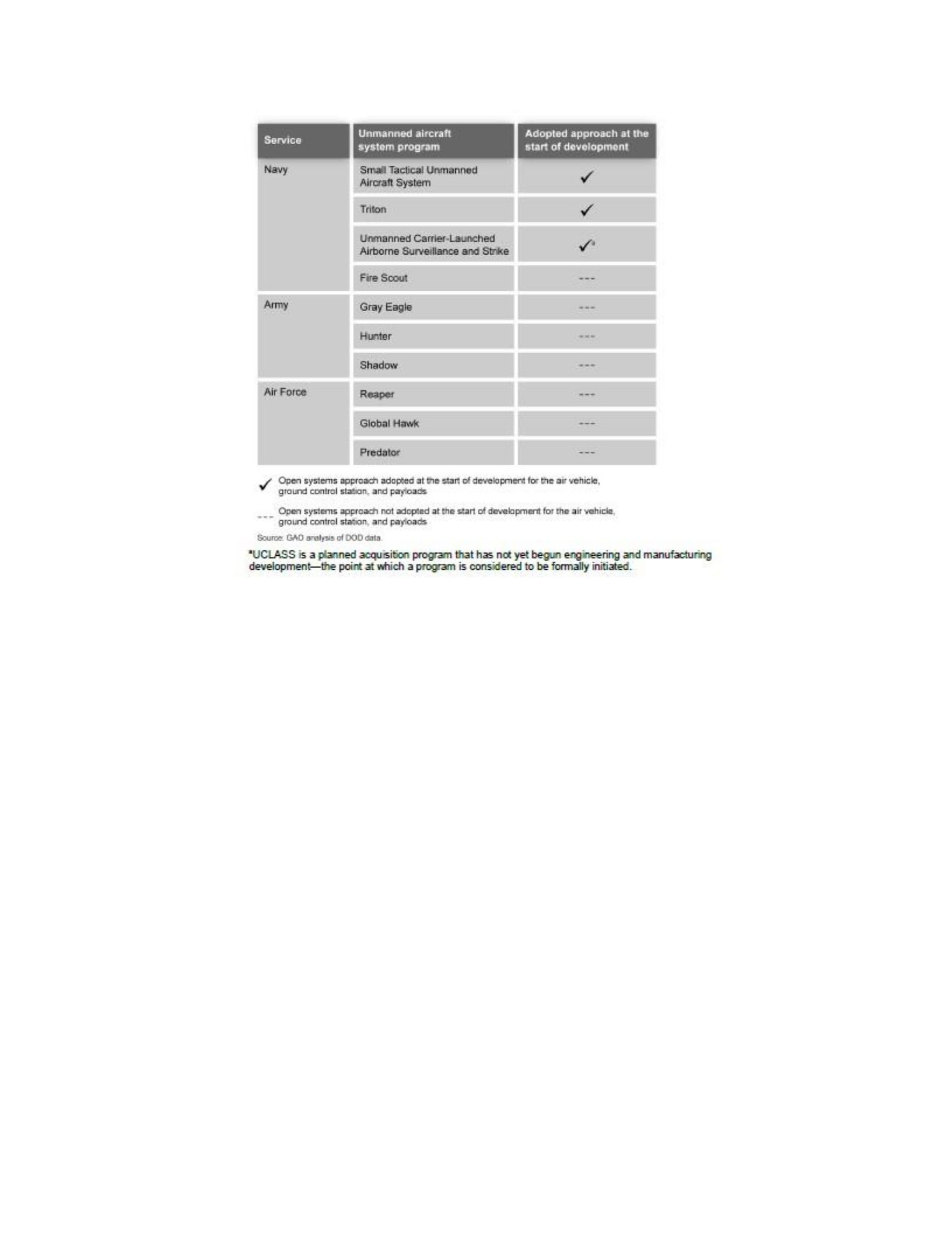
Figure 16: UAS Open Architectures (GAO, 2013: 12)

The GAO reported that for Triton, “Program officials estimated that software

testing could be reduced by as much as 66 percent compared to systems that do not have

an open system design, in part because the program does not have to test the entire

system when introducing new software or upgrades.” (GAO, 2013: 13) For the USAF, the

GAO found that that age and budget considerations prevented Predator and Global Hawk

from utilizing OSA, while Reaper only used OSA in the ground station. The GAO found

that service policy was available to promote OSA, so programs were not ignorant of the

requirement. The GAO reported that, among other things:

• The services must continue to make OSA a priority and monitor

implementation

• That programs “provide clear and consistent direction for its approach

and that programs plan for an open systems approach prior to the start of

development” (GAO, 2013: 19)

• “Contracts and requests for proposal should include appropriate language

that describes the open systems architecture, defines open standards, and

establishes requirements for control documents to ensure the government

retains rights for the identified key interfaces.” (GAO, 2013: 19)

The GAO findings show that the implementation of MOSA requires more than

just having the contractor develop a MOSA compliant implementation. Rather, the

program must develop the approach prior to any contract, and this approach must include

specific architecture requirements based on the programs business case.

A more recent study was conducted in 2016 by the MOSA Technical Standards

Working Group (TSWG) to explore the use of MOSA in Defense Acquisition Programs

(MOSA TSWG, 2016). The TSWG interviewed a large group of government program

offices, industry and academia, for a total of over 82 responses. The report covered a

range of topics, a few of the findings are summarized here.

• “All but four of the MDAPs and MAIS reported themselves employing a

MOSA approach.” (MOSA TSWG, 2016: 34)

This finding shows that programs are complying with the MOSA approach, or are

at least claiming to. However, merely claiming MOSA compliance is not enough. So the

TSWG investigated whether programs were measuring MOSA effects. They found:

• “MOSA measurement tools were cited as unknown or inadequate.

Inability to effectively measure results will hamper any efforts to move

toward MOSA benefits.” (MOSA TSWG, 2016: 8)

• “According to the senior leaders, with one or two exceptions, quantitative

measurement did not exist in programs implementing MOSA.

Measurement of modularity, openness, and overall success with MOSA is

based largely on the subjective judgment of subject matter experts.”

(MOSA TSWG, 2016: 9)

This study was continued by the MOSA Study Team, who prepared a report for

the Under Secretary of Defense for Acquisition, Logistics and Technology to support BBP

3.0. (MOSA Study Team, 2016). Without measurement tools or any way to quantitatively

measure progress, the Study Team was unable to determine how effective programs were

in implementing MOSA. It was unclear to the investigators what level of cost reduction

or schedule compression was achieved by MOSA compliant programs. As they began

investigating other reasons why programs are not experiencing the effects of MOSA, they

found:

• “Another common theme is the government’s lack of consideration of

lifecycle costs when making design decisions.” (MOSA Study Team,

2016: 9)

• “The Study Team recommends programs review the business case and

system design prior to every major contracting action to determine

opportunities for modular design.” (MOSA Study Team, 2016: 16) Both

studies were also interesting by what they didn’t find. Lack of standards

what found to be a barrier in less than 2% of responses. In addition, over

40% of respondents found that there were no gaps in standards for their

programs. In contrast, the largest barriers to using MOSA were lack of

resources and conflicting or unclear MOSA requirements. Both of these

concerns can be addressed with better understanding of how MOSA

requirements relate to both cost and capability.

Cost Effectiveness

Cost Effectiveness Analysis (CEA) is a key component of an Analysis of

Alternatives, as described in the Defense Acquisition Guidebook. (DAU, 2013) It’s

important to understand the distinction between cost effectiveness and cost benefit. “Cost

- effectiveness analysis is a technique that relates the costs of a program to its key

outcomes or benefits. Cost - benefit analysis takes that process one step further,

attempting to compare costs with the dollar value of all (or most) of a program’s many

benefits.” (Cellini and Kee, 2010: 493) In many fields, it is difficult or undesirable to put

a monetary value on the benefits of a system. This is especially true in military systems,

where the various measures of effectiveness are challenging to monetize. Consequently,

cost effectiveness is traditionally used more than cost benefit within the DoD.

In a CEA, both cost and effectiveness are calculated independently. Traditional

CEA performs multiple sub-analyses to account for each Measure of Effectiveness

(MOE). Once the cost and effectiveness are calculated for all alternatives for a given

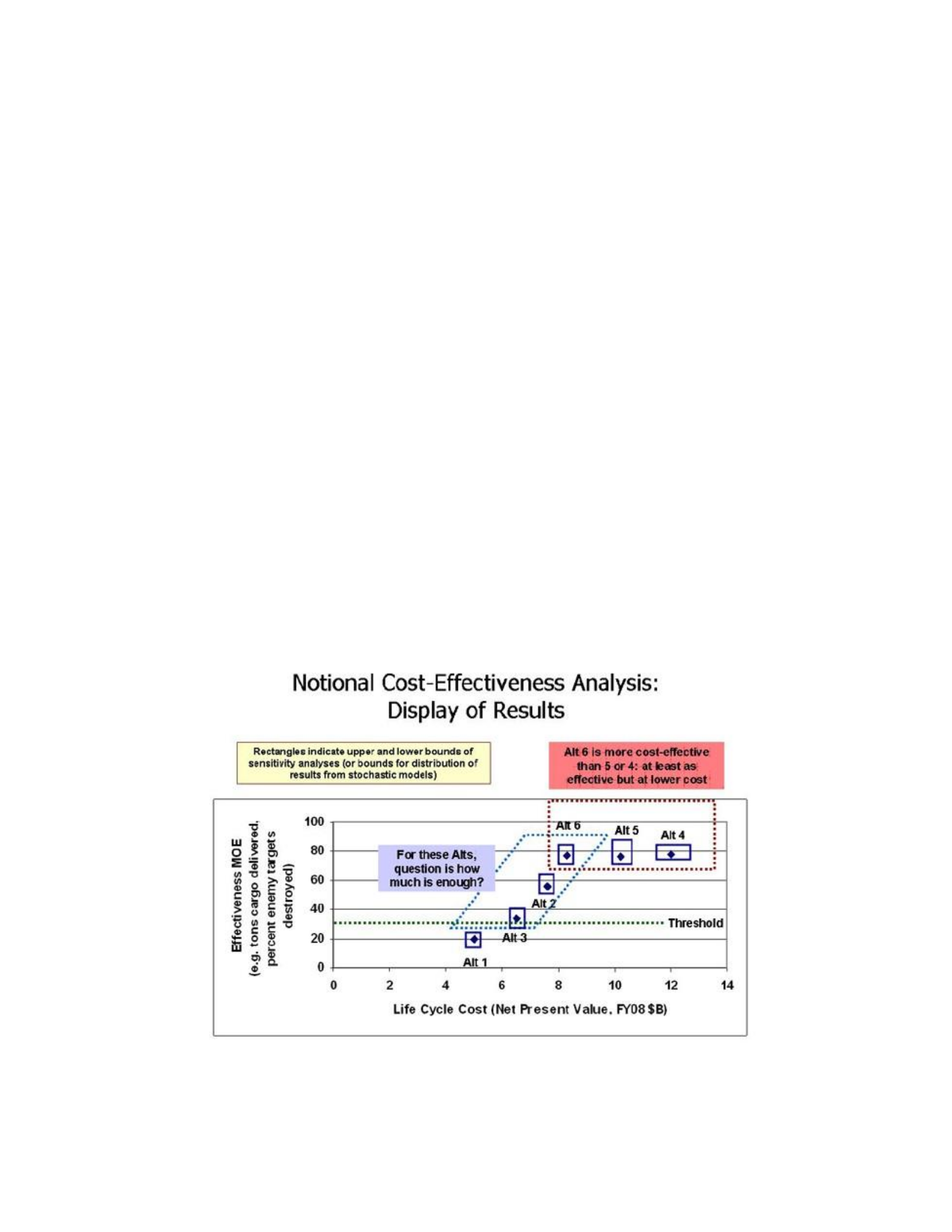
MOE, there are multiple ways to compare the alternatives’ performance. One method is

the scatter plot (Figure 17). In this case, there is a single plot for each MOE, and the

alternative is plotted against both cost and effectiveness.

Figure 17: Scatter Plot for a Notional Cost Effectiveness Analysis (DAU, 2013)

Another method of comparison is the cost effectiveness ratio (CER). The CER is a

method of directly comparing a quantitative measure, and is found by creating a ratio

between cost and a measure of effect. The traditional equation is: (Cellini and Kee, 2010:

493)

𝑇𝑇𝑇𝑇𝑇𝑇𝑇𝑇𝑇𝑇 𝐶𝐶𝑇𝑇𝐶𝐶𝑇𝑇

𝐶𝐶𝐶𝐶𝐶𝐶 =

𝑈𝑈𝑈𝑈𝑈𝑈𝑇𝑇𝐶𝐶 𝑇𝑇𝑜𝑜 𝐶𝐶𝑜𝑜𝑜𝑜𝐸𝐸𝐸𝐸𝑇𝑇𝑈𝑈𝐸𝐸𝐸𝐸𝑈𝑈𝐸𝐸𝐶𝐶𝐶𝐶

One example is from the medical industry: say that for a given treatment, it costs

$1000 to save 10 lives. The CER would be $100 per life saved. Using the reciprocal of

this equation is also common, as it is easier to evaluate programs within the context of a

specific budget. (Cellini and Kee, 2010: 493)

One concern with CER is that it can hide the effects of scale. For example, if

alternative A has 10 times the effect when compared to alternative B, but also 10 times

the cost, both alternatives will have the same CER. Thus the CER approach works best

when comparing alternatives of roughly similar scope.

Multi-Attribute Utility Analysis

A challenge of CEA is balancing multiple different effectiveness measures. In fact,

it is “typical to focus on one primary outcome in CEA.” (Cellini and Kee, 2010: 493)

There are multiple methods of evaluating effectiveness across multiple criteria, including

techniques such as the Weight Objectives Method (Cross, 2008), Value

Heirarchy (Parnell, et al, 2013), Multi-Attribute Utility Analysis (Keeney and Raiffa,

1993), Multiple Criteria (or Objective) Decision Making (various), Analytic Heirarchy

Process (Saaty, 2008), etc… All of these techniques vary, but they each have a

methodology for identifying three things:

1. A hierarchy of attributes

2. Normalized utility for each attribute

3. A weighting scheme across the attributes

Each technique focuses on different applications, and tailors the technique for

each purpose. For example, differences exist in the method of developing the attribute

hierarchy. Parnell describes two methods: the objective hierarchy and the functional value

hierarchy, whereas Keeney and Raiffa do not specify a method for developing an attribute

hierarchy and instead promote flexibility. Additionally, there are multiple terms utilized

for the actual parameters being evaluated. These include attribute, objective, criteria, and

measure of effectiveness.

Attribute Hierarchy

As stated above, a common aspect of multi-attribute decision making is the

generation of an attribute hierarchy. Traditionally, the analyst begins at the highest, most

abstract attribute or decision. Parnell recommends beginning with a statement of the

primary decision objective. He uses the example “Purchase the best car” as his purpose.

Keeney and Raiffa concur with this approach, while the NSA handbook recommends

starting at the definition of the system being procured (Continuing the example: “Sports

Car”). After the top attribute has been defined, the analyst decomposes that attribute into

smaller attributes. Many techniques exist for the decomposition process. Parnell’s

objective hierarchy (Figure 18) decomposes the attributes into desired objectives, such as

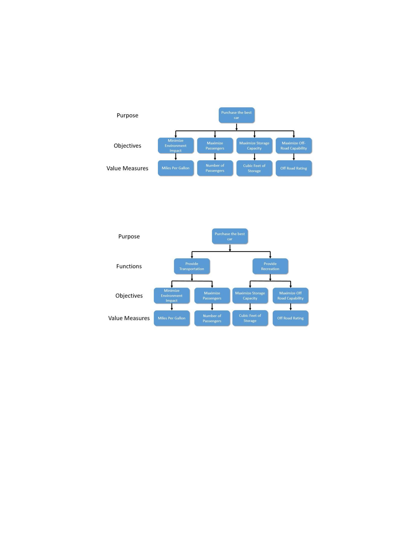
“minimize the environmental impact” and then to value measures. His functional value

hierarchy (Figure 19) decomposes the attributes into system functions, then to objectives

then to value measures.

Figure 18: Objective Hierarchy Applied to a Car Purchase

Figure 19: Functional Value Hierarchy Applied to a Car Purchase

The NSA handbook recommends decomposing the hierarchy according to system

characteristics.

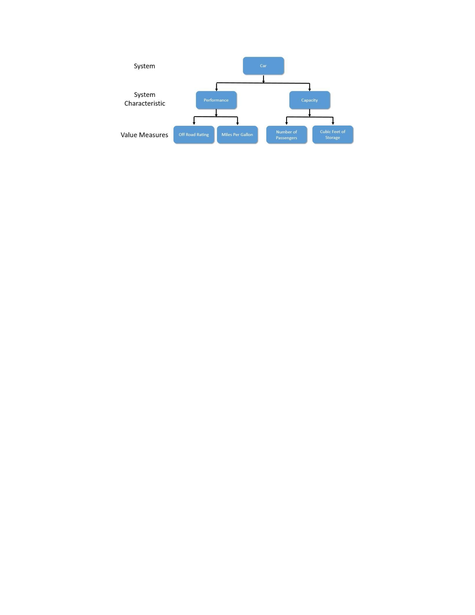
Figure 20: System Characteristic Attribute Hierarchy Applied to a Car Purchase

The lowest level attributes have many names. including bottom-level, leaf level,

and terminal branche. The widely accepted methodology is to continue to decompose

until the analyst reaches a leaf level attribute that is easily measurable and understood.

Most methods do not explicitly describe where to stop; rather, the analyst decides. In the

words of Keeney and Raiffa, ‘judgment must be used to decide where to stop the

formalization by considering the advantages and disadvantages of further specification.”

(Keeney and Raiffa, 1993: 43) A ‘bottoms up’ approach can be utilized either in addition

to or replacement of the top down approach. The bottoms up approach begins with known

value measures, and then builds up logical groupings at higher levels until a single

attribute is found.

The Additive Value Function

Along with the attribute hierarchy, the analyst must develop a method for

assessing the value of incremental changes in each attribute. Usually, this method is in the

form of a function that measures the change in utility as a function of incremental utility

and weights. One of the most commonly used is the additive value function, which is

used by Keeney and Raiffa, Parnell, Melese, and the NSA Handbook (among others).

Parnell describes the additive value function with the following equation: (Parnell, et al,

2013: 195)

𝑛𝑛

𝐸𝐸(𝑥𝑥) = 𝑤𝑤𝑖𝑖 𝐸𝐸𝑖𝑖(𝑥𝑥𝑖𝑖)

𝑖𝑖=1

Where

v(x) = the alternative’s value of x i = 1 to n is the index of the

value measure xi = the alternative’s score of the ith value

measure vi(xi) = the single dimensional y-axis value of an x-axis

score of xi wi = the weight of the ith value measure

The additive value function assumes mutual preferential independence, which

means that the result of the value function on one value measure does not depend on the

level of any other value measures. Because of this, the sum of all the weights must equal

1. It is important to note that the weights apply to the value measures.

The NSA guidebook develops a methodology for assigning weights using the

attribute hierarchy. Starting from the top of the hierarchy, the analyst assess the relative

importance of the attributes at each level. There are many methods used to assign these

weights. Blanchard and Fabrycky explain several methods used to work with stakeholders

to assign values. (Blanchard and Fabrycky, 2011: 186) One such method is to have

stakeholders select an importance rating based on a relative scale. For example, an analyst

may have a stakeholder assign each attribute an importance rating from 0 (completely

irrelevant) to 100 (absolutely vital). An additive weight is found by dividing each

attribute important rating by the sum of importance ratings.

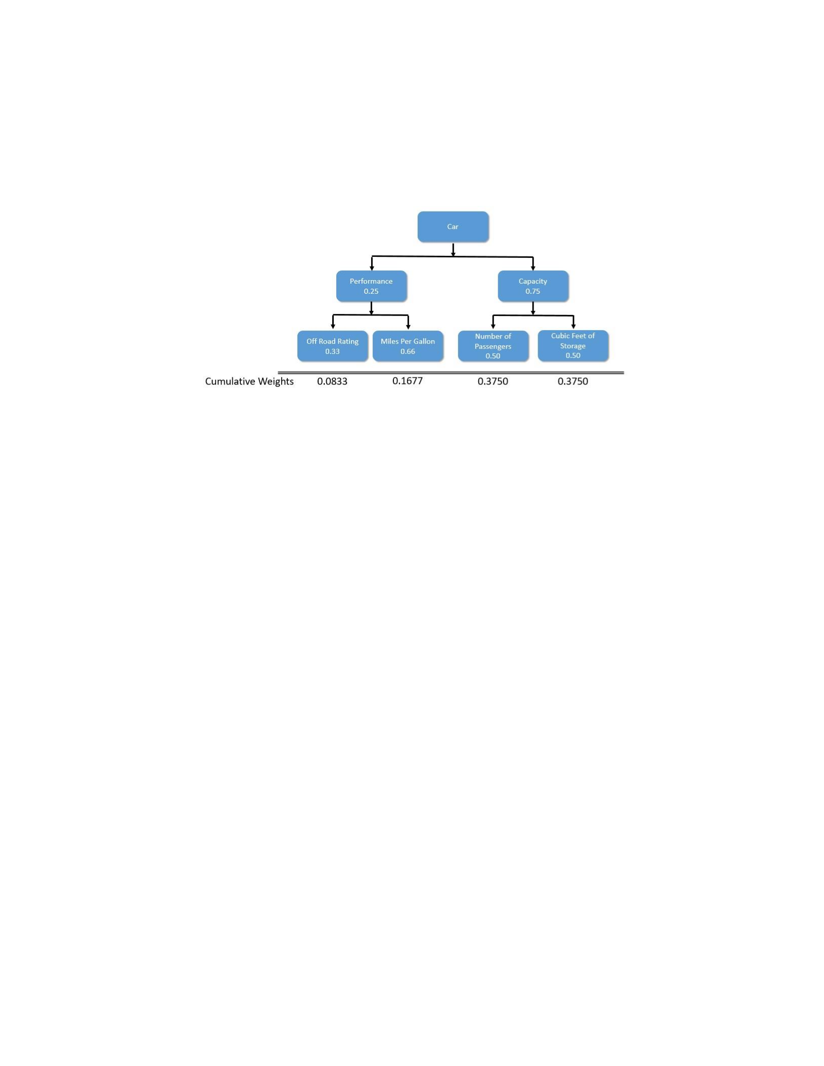
For each branch, assigned weights sum to a consistent value. The NSA selected

100, but it can also be other values. Figure 21 shows an example that uses a consistent

weight value of 1.

Figure 21: Attribute Hierarchy with Weights

To determine the cumulative weight for a leaf level attribute, the incremental

weights the leaf level attribute is multiplied by the incremental weights of each level

above it. The cumulative weight corresponds to wi in the additive value function.

Utility Curves

In addition to the attribute hierarchy and weighting scheme, the additive value

function requires the development of a value function for each leaf level attribute. The

value functions are often called Utility Curves. (NSA, 2000 and Melese, et al, 2015) For

each utility curve, the analyst identifies an attribute value that has zero utility. The analyst

also identifies an attribute value that achieves maximum utility, which is assigned a

normalized utility score. This score is usually either 1 (Melese, et al, 2015) or 100 (NSA,

2000), but can be any value that is consistently used throughout the analysis. In between

these two values, the analyst establishes a curve that defines the utility based on the

preference of the decision maker. These curves can take many shapes, based on the needs

of the individual program and the nature of the attribute. For example, there can be “all or

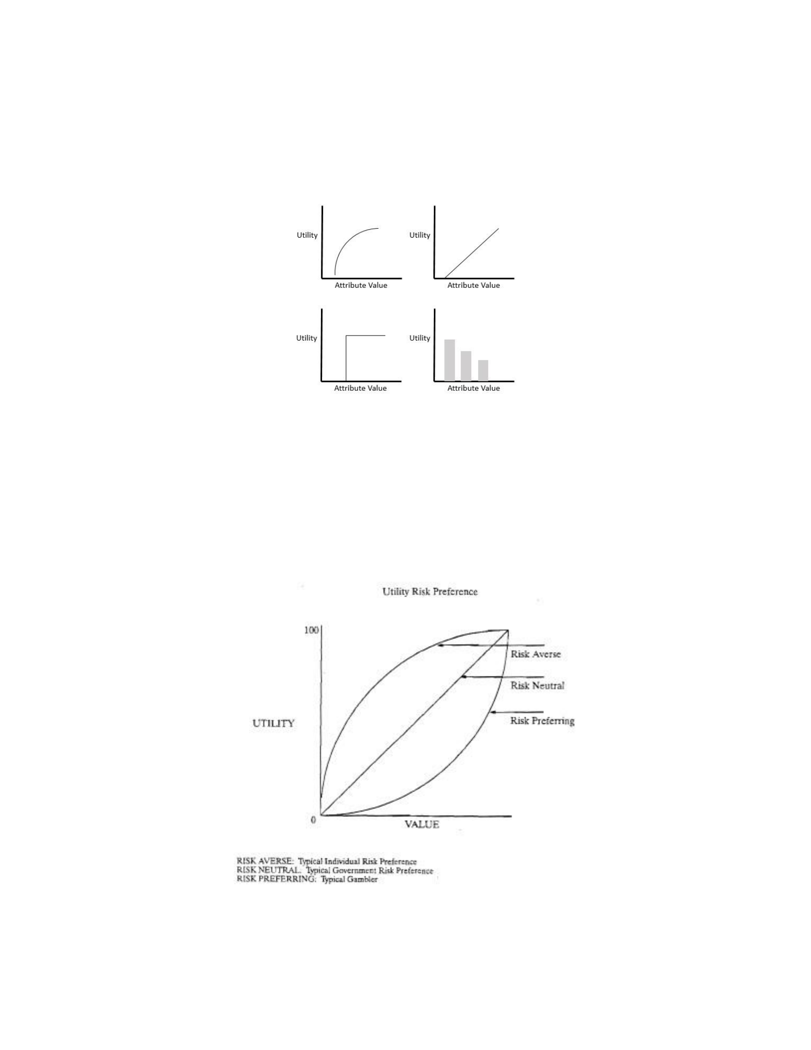
nothing” curves when the attribute either exists or does not. There’s no requirement that

the utility curve be continuous. Figure 22 shows some example curves.

Figure 22: Example Utility Curves

Figure 23 shows some notional curves that represents the acceptance of different

risk levels. The risk averse curve in figure 24 provides more utility for a given attribute

value, while the risk preferring curve provides less utility for the same value, driving

additional risk to the program by preferring harder to achieve attribute values.

Figure 23: Utility Risk Preference (NSA, 2000: 25)

The extant literature includes many methods to determine decision maker

preference and develop utility curves. For example, Melese, et al, note a method for

eliciting decision maker feedback using marginal information to develop cumulative

value functions.

Cost Estimation

In addition to measuring the effectiveness through MAUA, a CEA must also

evaluate cost. There are many methods for estimating costs, usually in specific domain

areas. An interesting example is the generic life cycle cost estimation shown by

Blanchard and Fabrycky (Blanchard and Fabrycky, 2011: 567-630). Almost all costs

break down into two primary components: parts and labor. Estimating the cost of parts is

a traditional exercise, often completed by analogy to an existing related part. This is

described in depth is various guides, including the NASA Cost Estimating Handbook

(NASA, 2008).

There are a wide variety of cost estimation methods for software, including

COCOMO II, Function Points methods, SEER-SEM, Putman’s Model, etc… COCOMO

II is a software cost model originally developed by Barry Boehm as COCOMO 81 in the

1980s, and developed into COCOMO II in the late 1990s. This model is based on a large

statistical population of software development programs, resulting in a fairly simple

general form equation: (Center for Software Engineering, 2000: 1)

𝐸𝐸

𝑃𝑃𝑃𝑃 = 𝐴𝐴 ∗ 𝑆𝑆𝑈𝑈𝑆𝑆𝐸𝐸∗ 𝐶𝐶𝑃𝑃

Where

PM: Person months

A: Calibration factor, which is 2.94 for COCOMO II

Size: Measure of functional size of a software module that has an additive effect on

software development effort

E: Scale factor(s) that has an exponential or nonlinear effect on software

development effort. It has a value of 0.91 ∗ ∑ 𝑆𝑆𝑆𝑆

SF: Scale factors

EM: Effort multipliers that influence software development effort

Utilizing the COCOMO II equations requires the use of a wide variety of factors

and multipliers. These are found in the COCOMO II Model Definition Manual. (Center

for Software Engineering, 2000) A larger discussion of COCOMO II is provided in

Appendix B.

Summary

As this chapter showed, the application of MOSA requires a broad systems

engineering approach, requiring knowledge in multiple subject areas. This chapter

addressed the investigation questions, beginning with a discussion of the Defense

Acquisition System, including the JCIDS and the CDD and SRD. MOSA was

summarized, along with a discussion of several MOSA related tools and an overview of

several MOSA implementation studies. The MOSA research showed that both tools and

metrics for MOSA application are lacking; resulting in many programs not knowing

whether they have a successful MOSA implementation or not. CEA theory was

developed, including MAUA, attribute hierarchies, the additive value function and utility

curves. Finally, the chapter concluded with a brief discussion of software cost estimation,

focusing on COCOMO II.

III. Methodology

Chapter Overview

This chapter builds upon the literature described in Chapter II and develops a

framework for evaluation the cost effectiveness of architecture alternatives. ACEF is

based on a cost effectiveness analysis that uses Multi-Attribute Utility Analysis (MAUA)

to relate multiple MOPs and derive a measure of operational utility. The ACEF also

develops a novel method of estimating MOSA relevant costs. This chapter develops the

ACEF in 6 steps:

1. Establish Business Strategy

2. Develop Program Reference Architecture

3. Create Alternatives

4. Compare Alternatives

5. Account for Uncertainty

6. Examine Results and Update Reference Architecture

Each of these steps is explained in detail, with particular emphasis on the

development of the Attribute Hierarchy, lifecycle reference utility profiles, architecture

alternatives, and cost estimation.

The Case for a Framework

As described in Chapter I, developing a standardized methodology for evaluating

the cost effectiveness of architecture alternatives will help programs realize the MOSA

benefits of improved utility, reduced lifecycle cost and decreased fielding time. To

perform the cost effectiveness analysis, methods of measuring both cost and effectiveness

must be developed.

For the Architecture Cost Effectiveness Framework (ACEF), effectiveness begins

with validated requirements, as provided by program KPPs and KSAs. These

requirements measures are validated through the JCIDS process, and thus have automatic

traceability to operational utility. In the ACEF, architecture decisions result in delivering a

system that is measured against these requirements.

Architecture decisions should result in better capability delivered faster and

cheaper. Consequently, the cost estimation for ACEF must take into account how the

architecture decisions, including the modular design of the system, definition of key

interfaces, and use of standards, affects the cost and utility of the system. Finally,

because faster capability delivery is a stated goal of MOSA, the ACEF must facilitate the

analysis of alternatives that deliver capability at different rates throughout the programs

lifecycle. This necessitates a continuous, rather than instantaneous, evaluation of both

cost and effectiveness.

The ACEF builds upon these themes to create a framework that evaluates cost

effectiveness of architecture alternatives throughout the program lifecycle, with emphasis

on directly relating the effects of architecture decisions to both operational utility (as

measured by validated KPPs and KSAs) and cost.

Step 1: Establish Business Strategy

An ACEF analysis must first establish the business strategy, which is common for

architecture alternatives being analyzed. Because ACEF takes advantage of MAUA, the

primary purpose of the business strategy is to identify the requirement Attribute

Hierarchy and associated utility curves. These curves are developed into Lifecycle Utility

Reference Profiles (LURPs) which document the expected utility for each leaf level

attribute over the programs lifecycle.

Develop Attribute Hierarchy and Cumulative Weights

While the ACEF does not require a specific approach to develop the Attribute

Hierarchy, the approach selected will result in a hierarchy of leaf level attributes that will

primarily be KPPs and KSAs from the approved capability documents. Some attributes,

such as the Net Ready KPP, will be split to create multiple value measures. Other

attributes may be omitted because they are not relevant to the comparison of architecture

approaches. For example, the system architecture choices (such as interface definition)

will not likely affect the system’s ability to withstand direct enemy weapons fire, and thus

will not affect the Force Protection KPP. In addition, APAs may be added to the Attribute

Hierarchy at the discretion of the program team. For example, some programs choose to

add sensor accuracy requirements, or computing latency requirements, to the SRD to

ensure appropriate capability delivery. The analyst should take care using nonJCIDS

validated attributes for two reasons: (1) the analyst must ensure that they directly add

operational utility, and (2) the analyst must ensure that the capability is not being “double

counted” in a KPP or KSA. For example, if the sensor accuracy APA is derived from a

target identification KPP, the target identification KPP should take precedence. However,

the analyst can make the sensor accuracy APA a leaf level attribute under a target

identification KPP branch.

There are multiple ways an ACEF analyst may design an Attribute Hierarchy. The

hierarchy itself may be composed of functions, objectives, characteristics, or other means.

For ACEF, it is expected that the analyst will use one of the following methods:

• Functional. The Attribute Hierarchy documents operational activities that

result in KPP or KSA leaf level attributes. If this approach is followed, it is

highly recommended to align with the DoD Architecture Framework

Operational View 5 (OV-5) Operational Activity Decomposition Tree. If

the OV-5 is used, branches that don’t result in relevant leaf level attributes

will have to be trimmed.

• Characteristic. The Attribute Hierarchy is broken down into system

characteristics that have associated KPPs, KSAs, or APAs.

• Logical. The Attribute Hierarchy is broken down into whatever

organization required to appropriately capture the preference between

KPPs, KSAs and APAs.

Both the functional and characteristic hierarchies will likely be accomplished by a

top down approach. In the case of the functional, the analyst would begin with the top

level activity, and then decompose into branches, and then into leaves. If using an OV-5,

this activity is largely accomplished. After the leaf level activities are identified, the

analyst will associate KPPs, KSAs or APAs as required. Leaf level attributes may not

have associated value measures, so the analyst should then follow with a bottoms up

approach to trim the tree of branches that do not have associated value measures. A

similar approach is taken with the characteristic method.

For the logical method, the analyst utilizes a bottoms up approach beginning with

the KPPs, KSAs and APAs, building a hierarchy that captures the preference between

attributes. For example, there may be a branch for all KPPs, a branch for all KSAs, and a

branch for all APAs. This would support a tiered preference where KPPs are always

preferred over KSAs, regardless of what activity or characteristic they would logically

belong to. A simple logical hierarchy could also be completely flat.

After the Attribute Hierarchy is developed, weights should be assigned using

methods such as the ones described by Blanchard and Fabrycky. Each branch will have

weights that sum to 1. This effort begins at the top level, and then each lower branch is

weighted, moving down until all leaf level attributes have been assigned weights.

At this point, the cumulative weight of each leaf level attribute is found by

multiplying the leaf level attribute weight by every branch level weight above it. These

weights will be used for each alternative throughout the ACEF analysis.

Define Lifecycle Utility Reference Profiles

Once all of the leaf level attributes have been defined and weighted, Lifecycle

Utility Reference Profiles (LURPs) must be generated for them. A LURP is a reference

model for an attribute that describes how both requirements and their associated utility

change throughout the lifecycle of the program. The LURP does this by defining a utility

curve that varies throughout the life of the program, usually by increasing or decreasing

threshold and objective values over time. The LURPs are similar in concept to design

mission profiles used in aeronautical engineering to calculate fuel consumption or

structural life, in that they both are used to have a common reference to estimate

performance rather than accurately predict the behavior of the system. In ACEF, the

LURPs are used to estimate utility across alternatives that deploy different design

implementations. To accommodate these design variations, the LURPs represent

requirements change over time rather than define specific modifications or upgrades. The

set of LURPs are applied to all alternatives, with each alternative’s design

implementations evaluated against the changing requirements described in the LURPs.

For example, a LURP for video resolution would define a requirement change from

Standard Definition video to High Definition video, rather than define a requirement for a

new Full Motion Video (FMV) system. This would allow for flexibility in developing

solutions that can take advantage of architecture alternatives. Using the video example,

an alternative with a proprietary FMV system could respond to the changing requirement

by replacing the entire FMV system. Another alternative with open interfaces within the

FMV system may respond to the same changing requirement by upgrading the video

encoder software only.

To create a LURP, the general profile for the attribute must be established. This

profile sets the shape of the utility curve for each future iteration. The attribute value for

the threshold and objective are set by the attributes themselves. In the ACEF, three basic

assumptions exist for all profiles: (1) Utility is measured from 0 to 100, (2) any value

below (or above for decreasing value cases) threshold has 0 utility, and (3) any value

above (or below for decreasing value cases) the objective has the maximum utility. With

these assumptions, the analyst determines two primary things: (1) the utility value of the

threshold, and (2) the shape of the utility curve between the threshold and the objective.

Figure 24 shows an example attribute utility curve. Some attributes will have discrete

results with coincident threshold and objective values. These attributes will have either 0

utility (either does not exist, or does not meet threshold) or 100 utility (either exists, or

meets threshold).

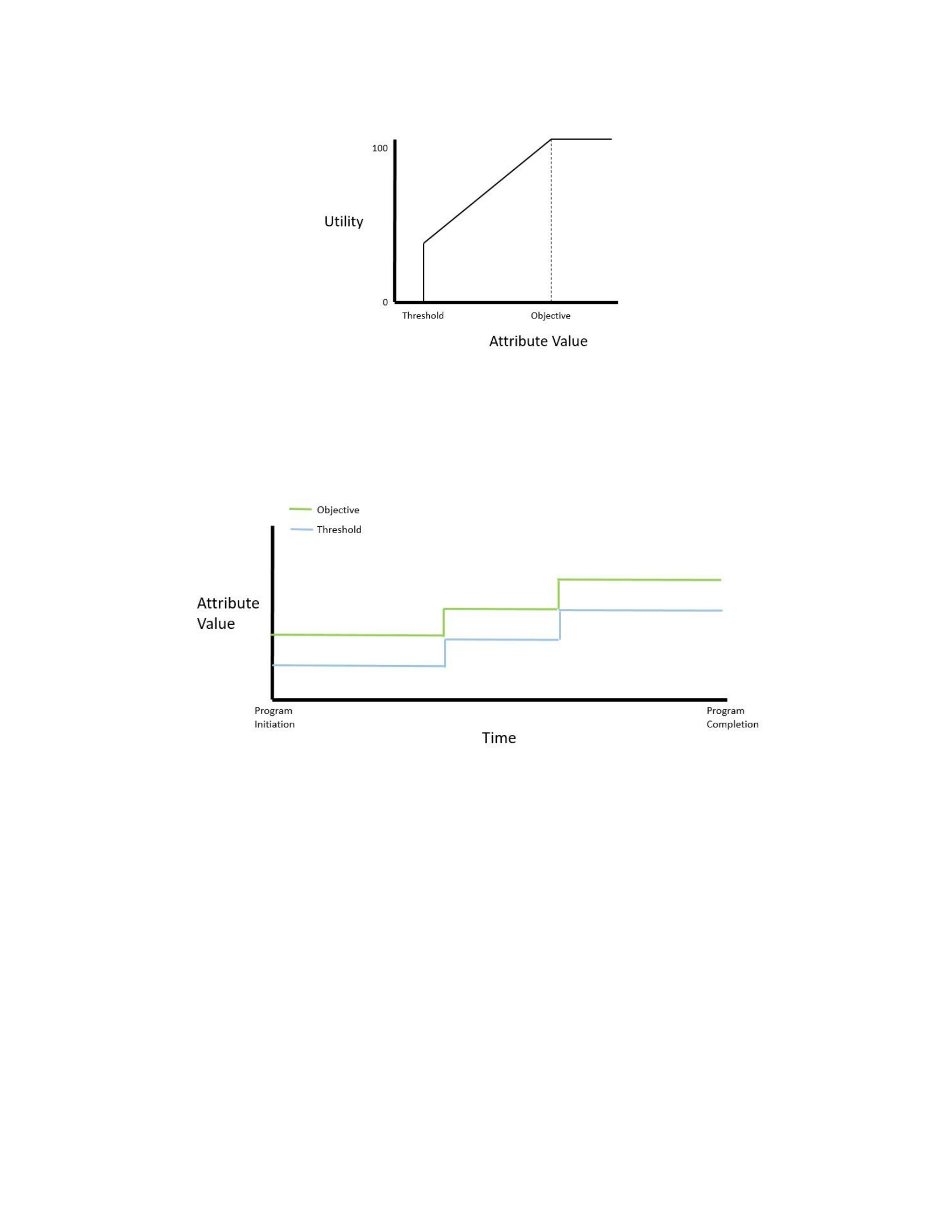
Figure 24: Example Utility Profile

The LURPs extend this profile by projecting the threshold and objective values

across the program life. Figure 25 shows an example LURP.

Figure 25: Example LURP

It is important to note that the LURP must start at program initiation, not at the

expected date of the first delivery. Starting at program initiation (rather than planned

IOC) allows for alternatives to propose an incremental approach, and accounts for each

alternative delivering utility asynchronously.

Step 2: Develop Program Reference Architecture

As discussed in Chapter II, reference architectures are important for a variety of

reasons. The ACEF requires the program either develop or tailor a reference

architecture for every acquisition. The reference architecture is an efficient way of

communicating the program’s desired approach, including key interfaces and the use

of standards. In ACEF, the reference architecture also serves as a baseline between

each analyzed alternative. At the very minimum, the reference architecture must:

• Define all external interfaces

• Define all architectural patterns that will apply across the alternatives

• Define minimal acceptable key interfaces within the system

• Propose minimal acceptable standards for key interfaces and components

• Propose any restrictions that the reference architecture will enforce. For

example, restricting a component from having any proprietary interfaces

The program should develop the initial reference architecture by conducting

market surveys of existing product lines and COTS/GOTS solutions. Any system

boundaries, interfaces and standards defined in the reference architecture are required to

be used for each of the ACEF alternatives. If the key interfaces are defined at a low level

of decomposition, then it may restrict the available product lines for use in the system.

The ACEF analyst should begin with a less constrained reference architecture avoid

overly constraining the alternatives, and then update the reference architecture with

additional constraints based on the results of the analysis. There are many tools available

to support the generation of the architecture, including the MDA and SysML tools

described in Chapter II.

Step 3: Create Alternatives

The primary purpose of the ACEF is to allow for analysis of multiple architecture

alternatives. These alternatives are made up of at least one design increment, but will

likely include multiple design increments to address changing requirements over the

lifecycle. Each design increment will be designed in accordance with MOSA principles,

and will include:

• The system architecture implementation, updated as required for the

design increment. The system architecture is required to conform to the

reference architecture.

• The components required to meet the system requirements. These may be

known (for off-the-shelf components), or notional (for new design or

modified components). It should be noted that the term component refers

to a coherent logical grouping of system hardware and software that will

be replaced or modified as a group. The component is the lowest level of

decomposition in ACEF.

• Identification and definition of all interfaces between all identified

components. These interfaces must at the minimum include the key

interfaces defined in the reference architecture. The alternative may

propose any type of interface, including key or proprietary. The alternative

should also clearly identify any standards that are fundamental to the

design

• Estimated system level capability. The alternative must provide an

estimated system level capability for each attribute in the business strategy

Attribute Hierarchy. This will be updated for each design increment.

A notional weapon system design increment is shown in Figure 26. Note that each

interface has 3 components: the interface definition (which describes the interface form,

fit, and function), and a ‘side’ for each component. The component side of the interface is

the aspect of the component that is responsible for executing the interface. This figure

will be used in following sections to describe the development of alternatives.

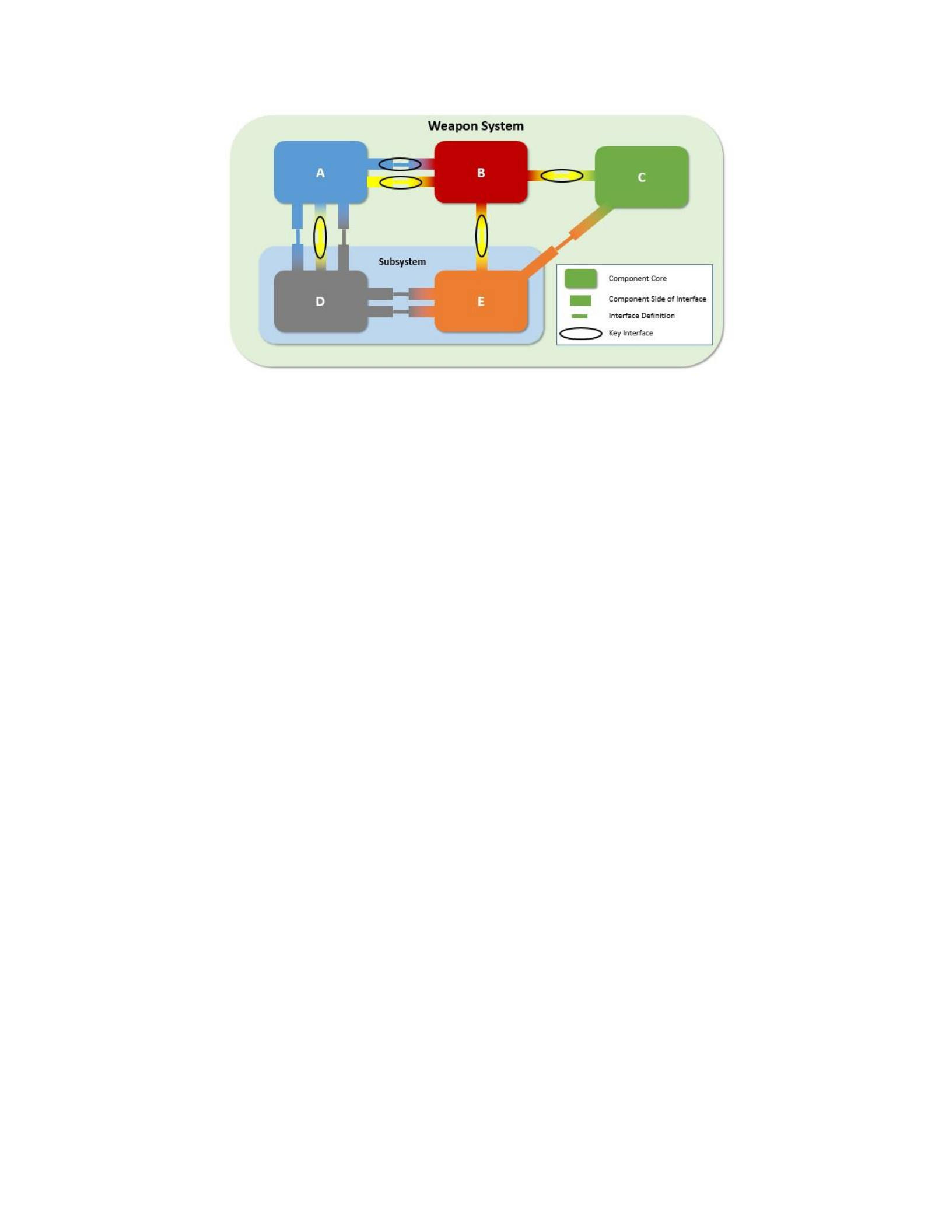
Figure 26: Notional Weapon System Design Increment Diagram

Each alternative develops its design increments independently. Alternatives are

not required to share design increment schedules unless specified in the common business

strategy.

Design Prime Alternative

A primary tenet of ACEF is to start with an alternative that conforms to the

reference architecture and prefers off-the-shelf (OTS) or non-developmental items (NDI)

in all cases. This alternative is called the Prime Alternative in ACEF. This is not only

consistent with the fundamental MOSA “plug-and-play” value proposition, but

specifically in accordance with both DoD policy and federal acquisition legislation which

requires the use of OTS components whenever possible. In addition to this guidance, the

prime alternative should also make use of existing DoD product lines where available.

To create the Prime Alternative, the program begins to functionally decompose the

system in accordance with the reference architecture. At each step of the functional

decomposition, the program performs a market survey to determine if an OTS component

exists that addresses some or all of the system requirements. At the completion of the

decomposition, the program selects a set of OTS components that best addresses the

system requirements. Where OTS components don’t exist, the program must decide either

to select the closest possible OTS component (if the component is required for system

operation), or defer integration of the component until a later design increment. The

prime alternative makes use of the best possible OTS components, with no guarantee that

the assembled components will meet all of the system threshold requirements. Once the

selection of OTS is complete, the program identifies the necessary interfaces and selects

standards as appropriate.

Along with architecture implementation, developing alternatives will require the

development of design increments. Because the program did not ensure that the initial

implementation met all system threshold requirements, the Prime Alternative must

develop design increments that modify the system to do so. For each design increment,

the program:

1. Determines which components need to be added or modified to meet to

achieve desired capability

2. Estimates the level of modification required for the component(s)

3. Identifies which interfaces require modification for each component

Figure 27 shows a notional design increment, where component A is being

replaced by component F. Interfaces 2 and 4 are key and utilize standards. Both

component A and F natively support the standard for interface 4, while both components

adapt for interface 2. Interface 3 uses the interface as defined by component D, so

component F must adapt to the interface. Interfaces 1 and 5 originally used component

A’s interface definition. The program: can (1) use the original definitions, and have

component F adapt to one or both, or (2) redefine the interfaces, and cause modification

to components B and/or D.

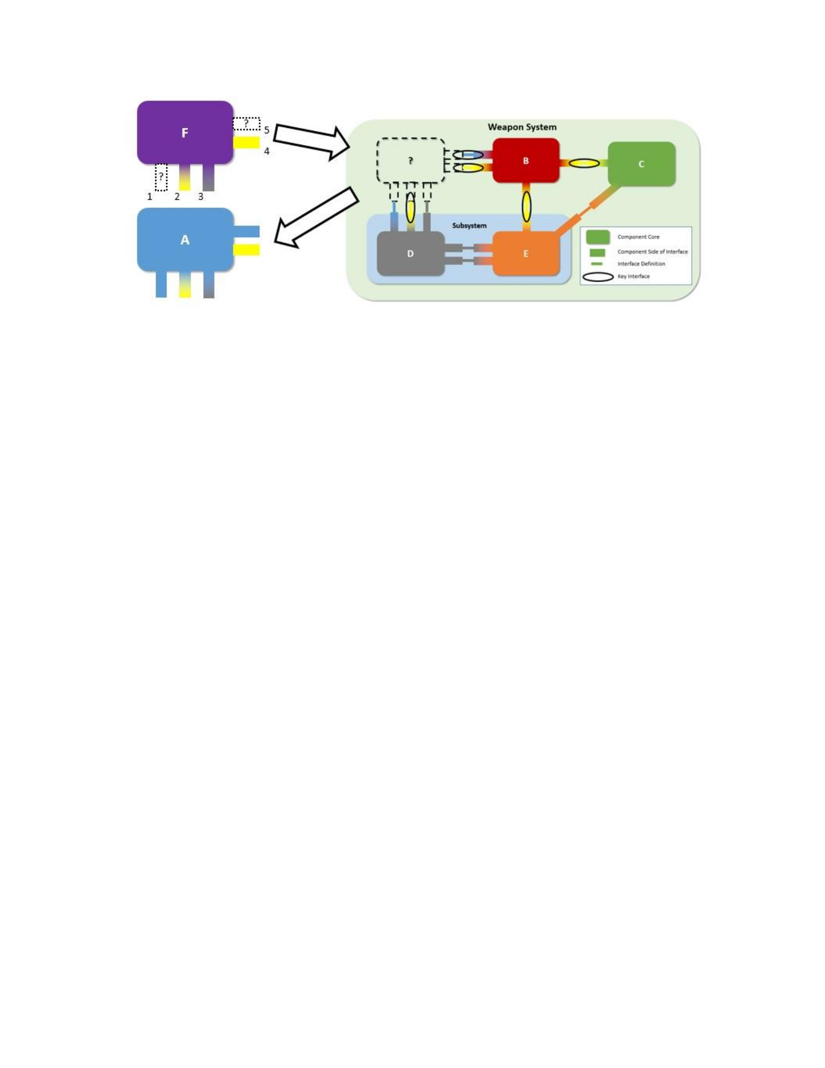
Figure 27: Notional Design Increment

The program repeats this process as necessary to develop sufficient increments to

meet all threshold requirements. In addition, the program should develop additional

increments throughout the lifecycle to address the changing requirements outlined in the

LURPs.

Create Alternatives

The maximum utilization of OTS components and interface standards reduces cost

for the initial capability delivery. Incremental capability delivery also facilitates faster

fielding. However, open interfaces, OTS components, and incremental delivery does not

ensure an effective MOSA design. These attributes must be combined using a modular

design that is tailored to the program’s business strategy. The ACEF is designed to

analyze multiple architecture alternatives to ensure that this is the case. Starting from the

prime alternative, the program should consider the following areas to modify to create

additional alternatives:

• Developmental components. Based on the expected level of development

of a component, it may make business sense to delay the delivery of the

initial capability. This is particularly beneficial when the OTS components

will not meet the threshold requirements.

• Further decomposition of components. Existing OTS components may not

provide the optimal level of openness for the long term business objectives

of the program. The program should investigate breaking down

components into smaller logical groups.

• Alternative interface definition. Depending on the expected design

increment delivery, there may be other options for defining interfaces. For

example, rather than a commercial standard, a government led or even

proprietary standard may be more beneficial.

• Design increment delivery. The program should investigate options for

scheduled design increments, including the timing as well as the packing

of the capability for each increment.

A program has wide flexibility to create alternatives, and is not limited to these

areas of investigation. The program should use both engineering and business judgement

to utilize the flexibility of ACEF with programmatic realism to choose a set of

alternatives.

Step 4: Compare Alternatives

The ACEF is designed to facilitate analysis of the cost effectiveness of different

architecture alternatives. As part of this process, the analyst will compare utility versus

cost, not just at a single point, but across the life cycle of the system.

Operational Utility

Operational utility is found by using MAUA and the additive value function. The

equation discussed in Chapter II is used here, in a modified form to align with ACEF

terminology:

𝑛𝑛

𝑈𝑈𝑇𝑇(𝐴𝐴) = 𝑤𝑤𝑖𝑖 𝐸𝐸𝑇𝑇,𝑖𝑖(𝐴𝐴𝑇𝑇,𝑖𝑖)

𝑖𝑖=1

Where

UT(A) = the instantaneous utility for time T for the capability provided by

alternative A.

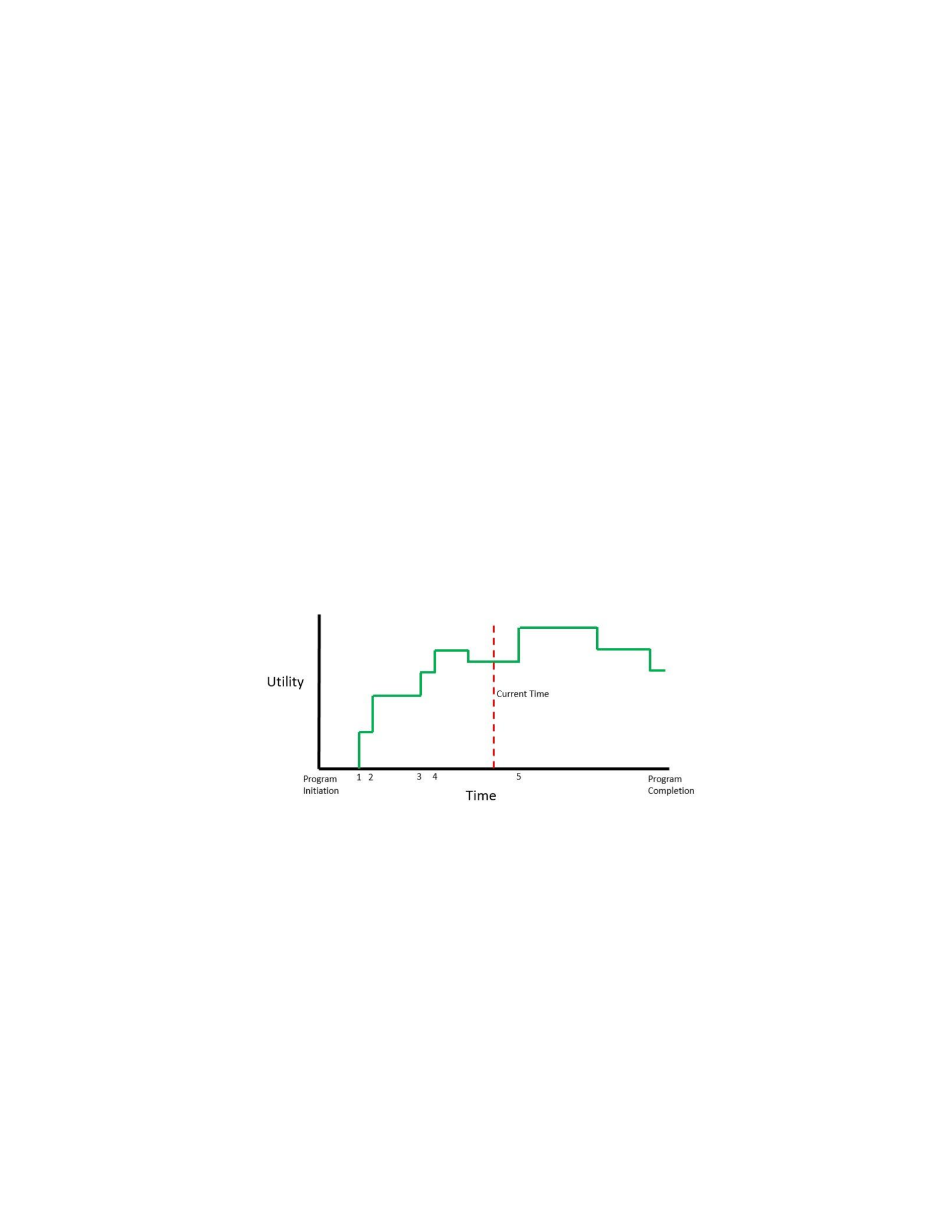
i = 1 to n is the index of the leaf level attribute

AT,i = capability associated with the ith leaf level attribute for alternative A at time

T.

VT,i(AY,i) = incremental utility associated with AY,i, given by the LURP at time T. wi

= the weight of the ith leaf level attribute, taken from the Attribute Hierarchy.

The operational utility is calculated annually, to align with the government

Planning, Programming, Budgeting, and Execution (PPBE) process. When one or less

modifications occur during a given year, the utility is calculated once to create the annual

utility. If needed, the year can be broken down into monthly segments to account for

multiple modifications that occur during the year, and thus multiple monthly utility

values. These monthly utility values are then added together and divided by 12 to create

the effective annual utility. Figure 28 shows a graph of instantaneous utility versus time,

with a single instantaneous time highlighted.

Figure 28: Instantaneous Utility

The instantaneous utility is useful for evaluating the operational utility of the

system at any given moment. However, using a single instantaneous utility calculation to

compare alternatives may mask overall utility trends. As Figure 28 shows, using the

instantaneous utility of the system at any single point does not indicate trends of the

operational utility of the system throughout its life.

Cost

In addition to the operational utility described above, cost models must be

developed to establish the ‘cost’ component of the ‘cost effectiveness’ analysis. The

ACEF does not attempt to accurately model all aspects of costs, but focuses on the areas

that will permit differentiation between alternatives. Consequently, this cost estimation

should not be used for other purposes without careful consideration.

The ACEF evaluates two types of costs: the cost to acquire a component, and the

cost to integrate the component. To generate the cost of the system, ACEF evaluates these

costs for each component, and then sums for all components. The ACEF governing cost

equation is:

𝐶𝐶𝐶𝐶𝐶𝐶𝐶𝐶𝐶𝐶𝑛𝑛𝐶𝐶𝑛𝑛𝐶𝐶𝐶𝐶

𝐶𝐶 = (𝐶𝐶𝐴𝐴𝐶𝐶 + 𝐶𝐶𝐶𝐶𝐶𝐶)

𝑖𝑖=1

Where:

C = the total cost

CAC = the Component Acquisition Cost

CIC = Component Integration Cost

This is shown in Figure 29, where the component is shown broken down into the

component core, and the component’s interfaces.

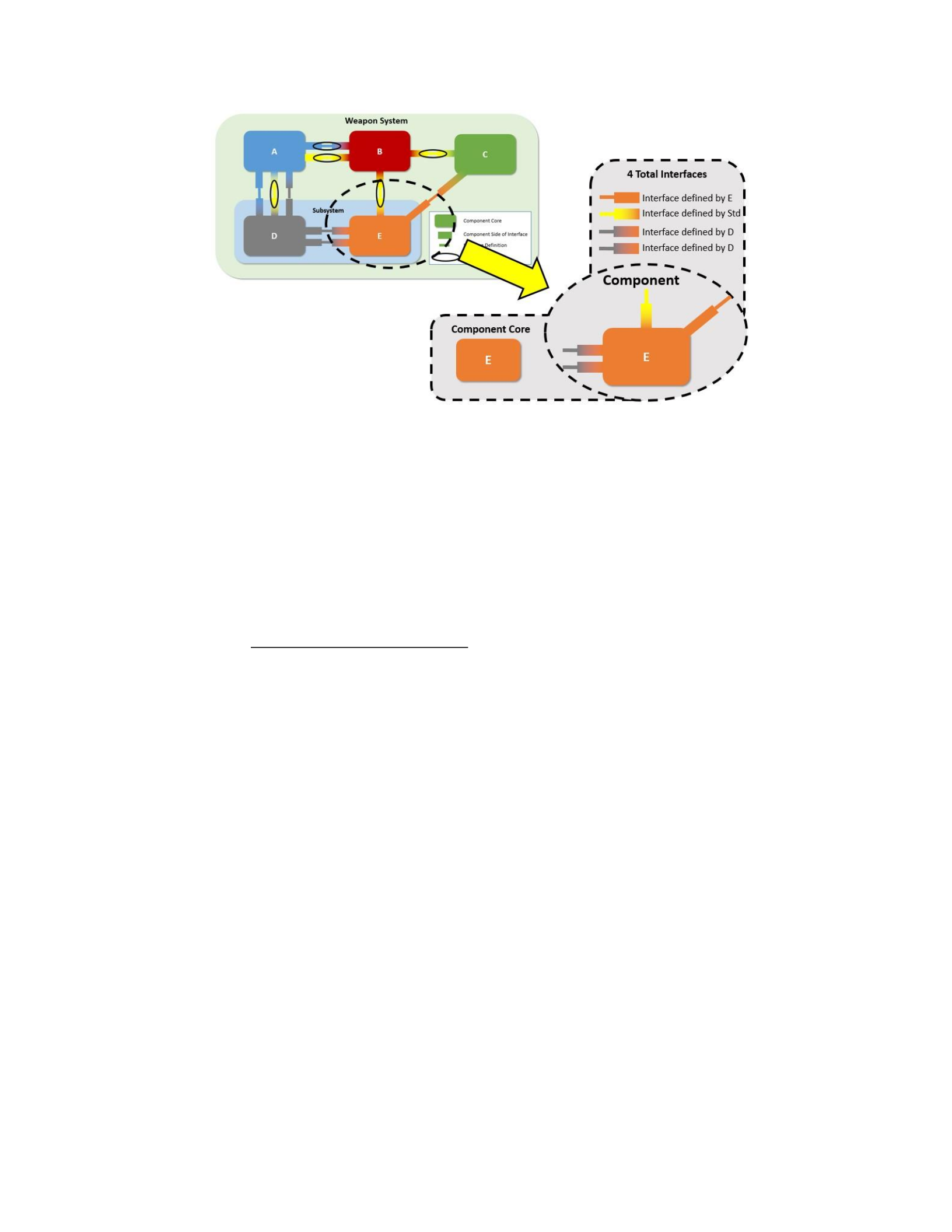
Figure 29: The Component Breakdown

The cost is evaluated any time the system is modified. At this time, the ACEF

does not account for the maintenance costs of the components or of the system as a

whole.

Component Acquisition Cost

The Component Acquisition Cost is the estimated cost to acquire the component

core, including the purchase cost as well as any non-recurring engineering associated with

modifying the component to meet the desired capability. This may include hardware

costs, but does not include any modifications needed to integrate it into the system. The

Component Acquisition Cost is defined by the following equation:

𝐶𝐶𝐴𝐴𝐶𝐶 = 𝐶𝐶𝐶𝐶 ∗ 𝐸𝐸𝑜𝑜 + 𝑁𝑁𝐶𝐶𝐶𝐶

CR refers to the component reference cost, which is the cost of a reference

component available to the program without modification. When OTS components are

used, CR refers to the actual cost of the component being acquired. If the component

requires modification, then the CR is modified by two factors to account for the

difference in price to acquire the real capability from the reference OTS component.

The calibration factor (cf) accounts for the difference between the purchase cost of

the reference component and the purchase cost of the actual capability. The cf only

calibrates the purchase cost, NOT the cost to modify the component. The cf can take into

price increases (cf > 1) or decreases (cf<1). Price increases may be caused by scenarios

such as diminishing manufacturing sources, shrinking supplier bases or other factors.

Price decreases may be caused by increasing market acceptance and competition, or to

reflect that fact that a modification requires updating an existing item rather than

replacing it. The cf can also represent an entirely new system that only uses the reference

cost as a starting point.

The cost cost to modify the component is accounted for by Non-Recurring

Engineering (NRE) costs, which take into account any directly funded engineering

necessary to modify the component. The NRE represents the “labor” component of the

CAC. NRE is only incurred when the program funds the modification: if a company

upgrades the component as part of an internal product line, NRE is 0. Likewise, if another

government program incurs the cost, NRE is also 0. For better or worse, if NRE does not

equal zero, the USG is not fully leveraging the plug-and-play OTS value proposition.

This concept is extended to new design components by selecting an OTS

component closest to the desired component. Once this is done, the program should

determine whether or not the program is required to pay to develop the component. If so,

the NRE should be estimated. Regardless of who pays to modify the component, the

calibration factor should be applied to determine the new purchase cost.

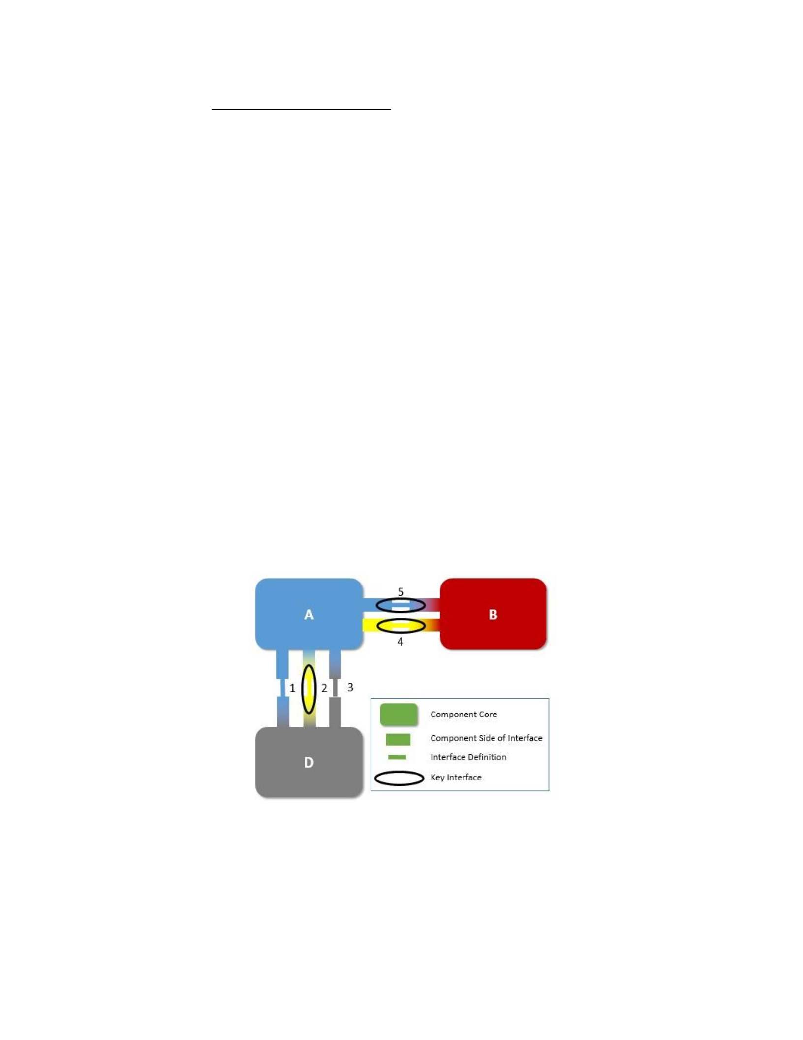
Component Integration Cost

As shown in Figure 29, each interface has an end associated each

component being connected. The Component Integration Cost (CIC) is found for every

component by evaluating the ends of all interfaces associated with the component, as

described by the following equation:

𝐼𝐼𝑛𝑛𝐶𝐶𝐶𝐶𝐼𝐼𝐼𝐼𝐼𝐼𝐼𝐼𝐶𝐶𝐶𝐶

𝐶𝐶𝐶𝐶𝐶𝐶 = 𝐶𝐶𝐶𝐶𝑗𝑗

𝑗𝑗=1

Where:

CIC = the Component Interface Cost

ICj = the Interface Cost at the jth interface of the component

The first evaluation is to determine whether or not the interface requires

modification. Figure 30 shows the initial integration of a notional system, consisting of

components A, B, and D.

Figure 30: Interface Changes

Table 3 shows a matrix of how the interface definition affects each component.

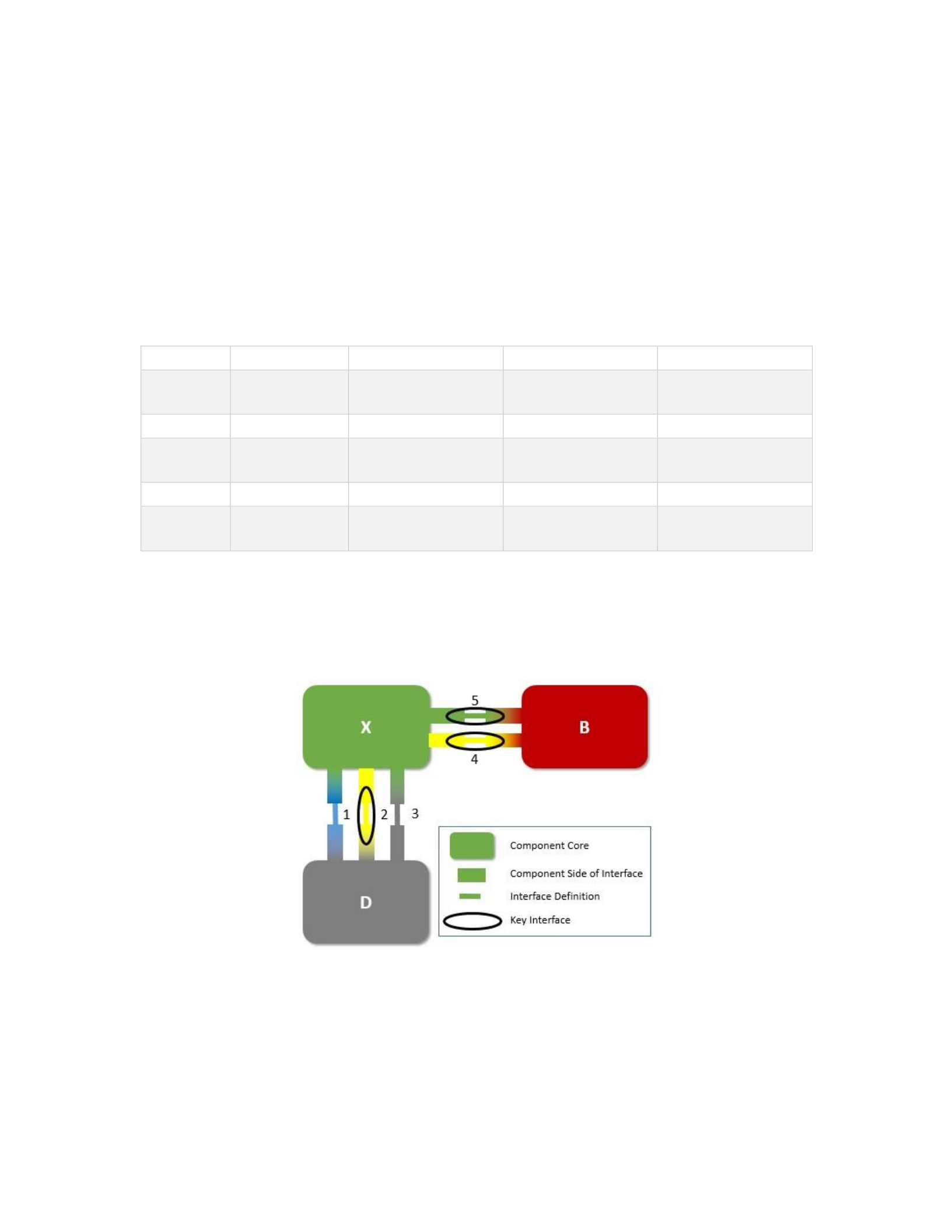
For example, for component A, the interfaces 2 and 3 will require adaptation because

component A does not natively support the interface definition, and thus additional cost,

while interfaces 1 and 5 will not because the system uses component A’s interface

definition.. Interface 4 does not require adaptation because component A natively

supports the interface standard.

Table 3: Interface Matrix

Interface

Defined By

Component A

Component B

Component D

1

Component A

No Change

N/A

Adapted

2

Standard

Adapted

N/A

Adapted

3

Component D

Adapted

N/A

No Change

4

Standard

No Change

Adapted

N/A

5

Component A

Adapted

N/A

Next, Figure 31 shows the same scenario, but with component X replacing

component A.

Figure 31: Notional Design Increment

Note that component X natively supports standards for both interface 2 and 4.

This design increment chooses to continue to use component A’s interface definition for

interface 1, accepting the additional adaptation to limit the changes required to

component D. In contrast, interface 5 is redefined to match component X’s interface

definition. Table 4 shows a matrix of how the interface definition changes affects each

component.

Table 4: Notional Design Increment Interface Matrix

Interface

Defined By

Component X

Component B

Component D

1

Component A

Adapted

N/A

No Change

2

Standard

No Change

N/A

No Change

3

Component D

Adapted

N/A

No Change

4

Standard

No Change

N/A

5

Component X

Adapted

N/A

This table shows a couple of important results. First, component D is completely

unchanged. The use of modular design and defined interfaces successfully isolated

component D from the replacement of component A. Component B had a single interface

change, due to the fact that the original interface was defined by Component A. Note that

component D had interfaces that did not change using both standard and non-standard

interface definitions. The use of standards (and definition of key interfaces) does not

guarantee an unchanging interface. The more widely accepted an interface is, the more

likely that a component will natively utilize it and not require adaptation during

integration. Also, the more information that is available to the program team about the

interface, the easier it is for the team to modify it. Using more open standards increases

the amount of information that is freely available.

For each interface that changes, the analyst selects a cost estimation method to

account for the level of effort to adapt the component to the interface definition.

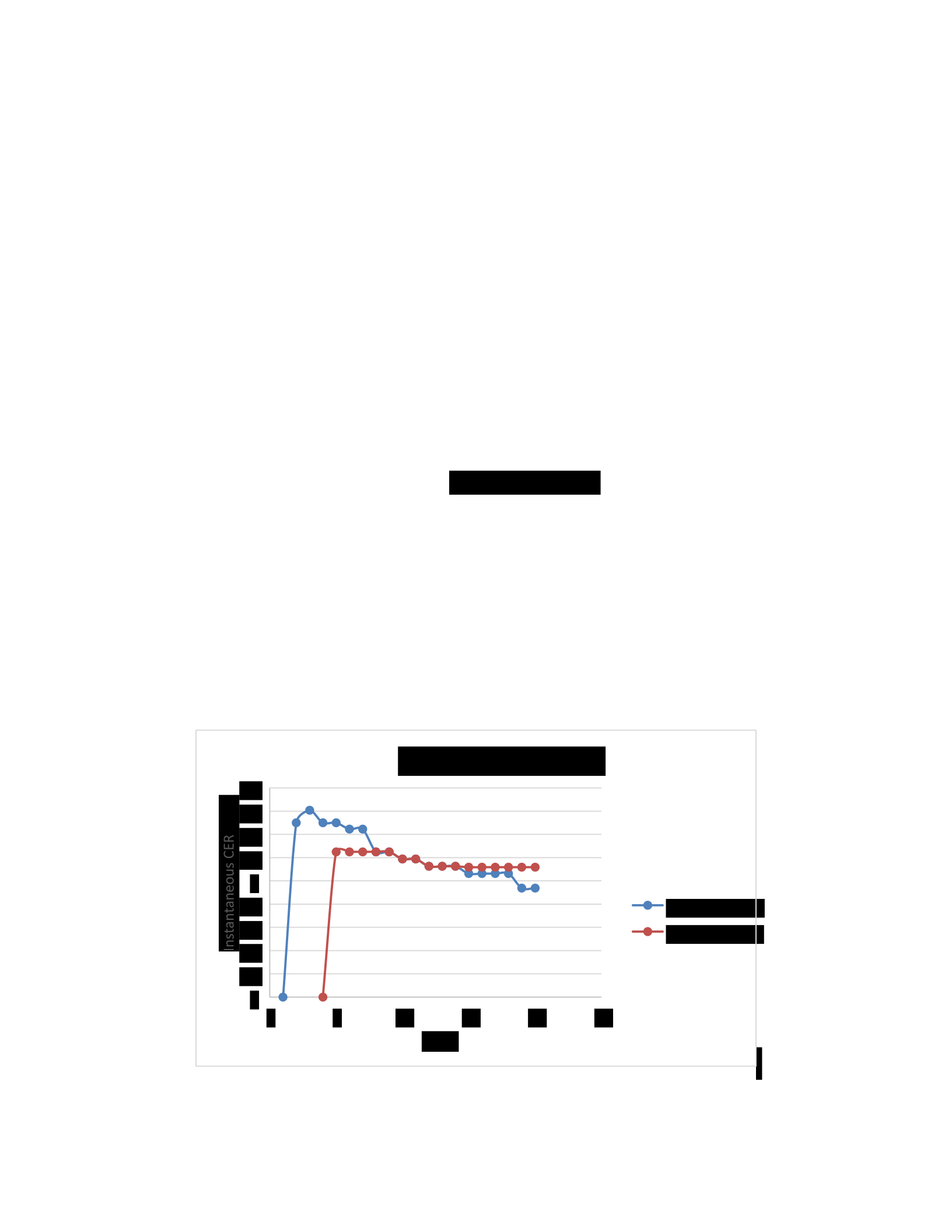
Currently, ACEF considers only software interfaces when determining cost. The author

will use the COCOMO II equation, which calculates an effort measured in Person

Months. This level of effort is then multiplied by a general fully burdened cost rate

indicative of industry to result in cost. This will be shown in Chapter IV.

Cost Effectiveness

The basic metric used to evaluate the alternatives is cost effectiveness ratio (CER).

The Instantaneous CEF (ICER) can be found by the utility of a given time by the total

cost to date:

𝐶𝐶𝐶𝐶𝐶𝐶𝐶𝐶𝐸𝐸𝑈𝑈𝑇𝑇 𝑈𝑈𝑇𝑇𝑈𝑈𝑇𝑇𝑈𝑈𝑇𝑇𝑈𝑈

𝐶𝐶𝐶𝐶𝐶𝐶𝐶𝐶

This metric shows the alternative cost effectiveness at the given time. However, it

does not account for the utility of capability delivered at any time other than the current

time. This makes it difficult to use to compare multiple alternatives, each of which may

deliver capability at different times. To do this, the metric can be plotted against time for

each of the alternatives, as shown in Figure 32.

0

0.2

0.4

0.6

0.8

1

1.2

1.4

1.6

1.8

0

5

10

15

20

25

Year

ACEF Comparison

Alternative A

Alternative B

Figure 32: ICER Comparison

Figure 32 shows that Alternative A develops utility faster, providing operational

utility for 3 years before the initial capability delivered by Alternative B. Alternative B,

however, provides more operational utility later in the program’s lifecycle.

While this graph shows the effect of architecture alternatives, it requires

subjective judgment to interpret, as both Alternative A and Alternative B are preferred in

different phases of the program. To permit more objective analysis, another metric is

used: lifecycle cost effectiveness ratio (LCER). This metric is simple to calculate:

∑𝐿𝐿𝑖𝑖𝐼𝐼𝐶𝐶 𝐶𝐶𝐶𝐶𝐶𝐶𝐶𝐶𝐴𝐴𝑛𝑛𝑛𝑛𝐴𝐴𝐼𝐼𝐴𝐴

𝐿𝐿𝐶𝐶𝐶𝐶𝐶𝐶 =

𝐿𝐿𝑈𝑈𝑜𝑜𝐸𝐸 ∗ ∑𝐼𝐼𝑛𝑛𝐼𝐼 𝐶𝐶𝐼𝐼𝑛𝑛𝐼𝐼

Where:

ICERAnnual = the Instantaneous CER, calculated annually

Life = the life of the program

Inc = the design increment

CInc = the Total Cost for design increment Inc

For the example above, Alternative A had an LCER of 71.25 per $M per year,

while Alternative B had an LCER of 70.25 per $M per year. Alternative A averages more

utility per dollar per year, meaning that on average, it will produce a more cost effective

solution than Alternative B. The program team will determine whether or not this

difference is significant based on their overall program objectives.

Step 5: Account for Uncertainty

Single comparisons are subject to various estimates that introduce unquantified

uncertainty. This uncertainty must be analyzed to ensure that the results are not unduly

sensitive to assumptions about user preference or future requirements. Sensitivity analysis

is described in many places in the extant literature (see NSA, 2000 and Parnell, 2013) and

the general purpose is to “assess the impact on value of changing each uncertain input

across its range of uncertainty” (Parnell, 2013: 189). The general technique is to identify

variables with uncertainty, identify low, nominal and high values for the variables, and

then evaluate the system for each variable. This evaluation is done by performing the

calculation using the off-nominal value for a single variable, and keeping the remaining

variables nominal. This process is repeated for each uncertain variable. The behavior of

the total calculated value as each variable is changes is investigated to determine if the

total value is sensitive to that variable.

Cumulative Weight Sensitivity Analysis

The first area of uncertainty to address is decision maker capability requirement

preference. This uncertainty occurs when decision makers do not explicitly apply their

priorities when assigning different attributes; or, if they do prioritize, if they don’t assign

quantitative values for their preference. Therefore differences between the values they

assign to the Attribute Hierarchy and their actual priorities for delivered system

capabilities arise. To account for this uncertainty, the weights in the Attribute Hierarchy

should be varied, the analysis re-run, and the LCER values compared to determine

whether the alternatives are sensitive to these changes. In particular, the analyst should

look for instances where the alternative preference order changes

Lifecycle Utility Reference Profile Sensitivity Analysis

In addition to the weights, the analyst should determine the alternatives’

sensitivity to the LURPs. The LURPs are designed to account for changing requirements

throughout the program’s lifecycle. However, while attributes such as KPPs, KSAs, and

APAs are explicitly defined and validated for the initial capabilities, rarely are future

threshold and objective values explicitly defined. Rather, future upgrades are traditionally

treated as separate acquisition activities, with new requirements created separately. In

contrast, the LURPs are not intended to accurately predict future requirements changes;

rather, they are intended to acknowledge the requirement that system utility should

improve in general across the lifecycle, and provide a common reference for evaluating

the alternatives. Despite this, it is important to vary the threshold and objective values of

the LURPs to ensure that the ACEF results are not sensitive to a particular LURP

configuration. To accomplish this, the threshold and objective values are varied for a

single LURP at a time, and the analysis is re-run.

Step 6: Examine Results and Update Business Strategy and Reference Architecture

After the analysis has been run, the business strategy and reference architecture

should be updated to reflect the lessons learned. For the business strategy, the program

should ensure that all selected attributes support the discrimination between alternatives

and ensure that the LURPs are appropriate for the analysis. If there are attributes that do

not add value to the analysis, they should be removed and the analysis re-run. If any

particular LURP drives the analysis, the analyst should consult SMEs in that area to

verify that the LURP represents realistic changes in the attribute requirement.

While the reference architecture should be updated based on the results obtained

through the ACEF, the exact areas to update will depend on how the reference

architecture was constructed. Some areas to consider are:

• Breakdown of components. The analyst should focus on specific design

increments that stress particular design patterns. If they show localized

cost effectiveness, it may be productive to investigate combining these

patterns with other alternative characteristics.

• Selection of standards. Use of standards is generally preferred. However,

the analyst should investigate how use of a particular standard affects

other aspects of the design. If a standard is selected because a given

component type widely utilizes it, but other related components do not, it

may not be cost effective overall. Another similar standard may be more

cost effective.

The ACEF can be executed in multiple iterations, based on feedback from

stakeholders. The result of ACEF should be a stable and mature business strategy and

reference architecture as input to the contracts generation process.

Summary

This chapter started with a discussion of the case for a cost effectiveness

framework. Next, the ACEF was developed in six steps, beginning with establishing the

business strategy. This included developing an Attribute Hierarchy and a set of LURPs.

Next, the ACEF developed a reference architecture, followed by the creation of a set of

architecture alternatives. After they were developed, the alternative were compared by

calculating both operational utility and lifecycle cost, resulting in a cost effectiveness

ratio. These calculations were then varied to account for uncertainty, before the program

examined the results and updated the reference architecture.

IV. Analysis and Results

Chapter Overview

Chapter IV details the general procedure described in Chapter III and implements

the procedure using a notional program called Program X. A notional program was

utilized to allow for an illustrative example that does not have operational security

concerns. Program X will use the ACEF analysis to evaluate three architecture

alternatives, describing each step in detail to further explain the application of the ACEF.

Finally, the investigation questions will be revisited and explicitly addressed.

Program X Overview

Program X will develop an Intelligence, Surveillance and Reconnaissance (ISR)

payload that will be installed onto a manned COTS aircraft. The primary mission of

Program X is to support finding, fixing, and tracking targets using Multi-Intelligence

(Multi-INT) capabilities. Secondary missions are to collect Full Motion Video (FMV)

imagery and Moving Target Indication (MTI) radar detections for pattern of life

intelligence generations.

To accomplish these missions, the system must provide certain key capabilities.

Program X was assumed to have a set of validated requirements documents. Of interest to

the Program X analysis is the Capability Development Document (CDD), which included

the following KPPs.

Table 5: Key Performance Parameters for Program X

EO Video Resolution

System shall collect and provide to analysts EO video.

Threshold: 480p

Objective: 1080p

IR Video Resolution

System shall collect and provide to analysts IR video.

Threshold: 480p

Objective: 1080p

Radar MTI

Detection Coverage

System shall collect and provide to analysts MTI

detections.

Threshold: 625 square kilometers

Objectives: 1225 square kilometers

Disseminate FMV

Data

System shall disseminate FMV video through

SATCOM. Threshold = objective.

The Electro-Optical (EO) video will provide primarily day FMV, while the

Infrared (IR) will provide night capability. The Radar MTI will provide increased ability

to track targets through visual occlusion, including clouds. Finally, the dissemination of

the FMV data will allow for situational awareness for decision makers worldwide, and

support for reach back intelligence exploitation.

In addition to the KPPs, the CDD also includes a variety of KSAs (Table 6). The

radar tracker will take the detections from the MTI system and stitch them together to

form contiguous tracks, greatly increasing the analyst’s ability continuously monitor their

targets. Subsystem A will be a notional subsystem for identifying and geo-locating

targets. Additional information about Subsystem A is not required for this analysis.

Disseminating all other data further will support both situational awareness and

reachback intelligence exploitation.

Table 6: Key System Attributes for Program X

Radar Tracker

System shall utilize MTI data to create tracks.

Threshold = objective.

Subsystem A

Geolocation

Accuracy

System shall identify and geolocate targets using

Subsystem A.

Threshold: 25 meter allowable error

Objective: 10 meter allowable error

Disseminate MTI

Detections

System shall disseminate MTI detections through

SATCOM. Threshold = objective.

Disseminate

Subsystem A Data

System shall disseminate Subsystem A data through

SATCOM. Threshold = objective.

Disseminate Radar

Tracks

System shall disseminate radar tracks through

SATCOM. Threshold = objective.

In addition to the initial requirements, it is anticipated that multiple blocks of

modifications will be developed to deliver capability in the face of changing

requirements. Specifically, it is anticipated that sensor requirements will continue to

progress. Because of this, an effective MOSA strategy is considered vital to Program X.

Step 1: Establish Business Strategy

Attribute Hierarchy

When generating the Attribute Hierarchy, Program X determined that KPPs are

inherently more important than KSAs, by a ratio of 60/40. This breakdown was used to

develop the Attribute Hierarchy into two separate branches with the KPPs and KSAs

arranged as leafs in their respective branch (Figure 33). Next, the relative values for leaf

level attributes in each of the branches were found by using the method described by

Blanchard and Fabrycky. The Program X team assigned an importance rating of 100 for

the most important attribute in the branch. Each of the other attributes was assigned an

importance rating (from 0 to 100) that corresponded to the operational value that attribute

would provide. Using this 0-100 scale, the additive weight was found by normalizing the

respondent weights using the following equation:

𝐶𝐶𝐶𝐶𝐼𝐼

𝐴𝐴𝑊𝑊𝐼𝐼 = ∑ 𝐶𝐶𝐶𝐶𝐼𝐼

Where:

AWa = Additive Weight of attribute a

IRa = Importance Weight of attribute a

The results of the survey and normalization are shown below (Table 7 and Table

8).

Table 7: Program X KPP Attribute Weights

Importance

Rating

Additive

Weight

EO Video Resolution

100

0.3125

IR Video Resolution

80

0.2500

MTI Detection

Coverage

50

0.1563

Disseminate Video Data

90

0.2813

Table 8: Program X KSA Attribute Weights

Respondent

Weight

Hierarchy

Weight

Radar Tracks

80

0.2192

Disseminate MTI Detections

60

0.1644

Disseminate Radar Tracks

50

0.1370

Disseminate Subsystem A Data

75

0.2055

Subsystem A Geolocation

Accuracy

100

0.2740

Using these results, the Attribute Hierarchy was developed:

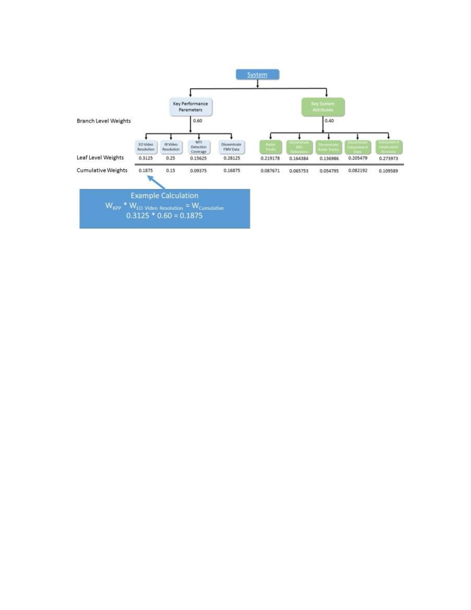
Figure 33: Program X Attribute Hierarchy

Lifecycle Reference Utility Profiles

After the Attribute Hierarchy, the other component of the business strategy is the

development of the LURPs. Program X developed two classes of LURPs: continuous,

and discontinuous. The continuous LURPs represent attributes than can be measured

continuously and have values that vary throughout their value range. The continuous

LURPs for Program X followed the general pattern shown in Figure 24. The threshold

value was assigned a utility of 50 and with any value lower than threshold was assigned 0

utility. Meanwhile, the objective value, and any values above objective, received a utility

of 100. Any value between the threshold and objective was assigned a utility value

following a linear curve between (threshold, 50) and (objective, 100). The following

graphs show the individual LURPs for each continuous attribute.

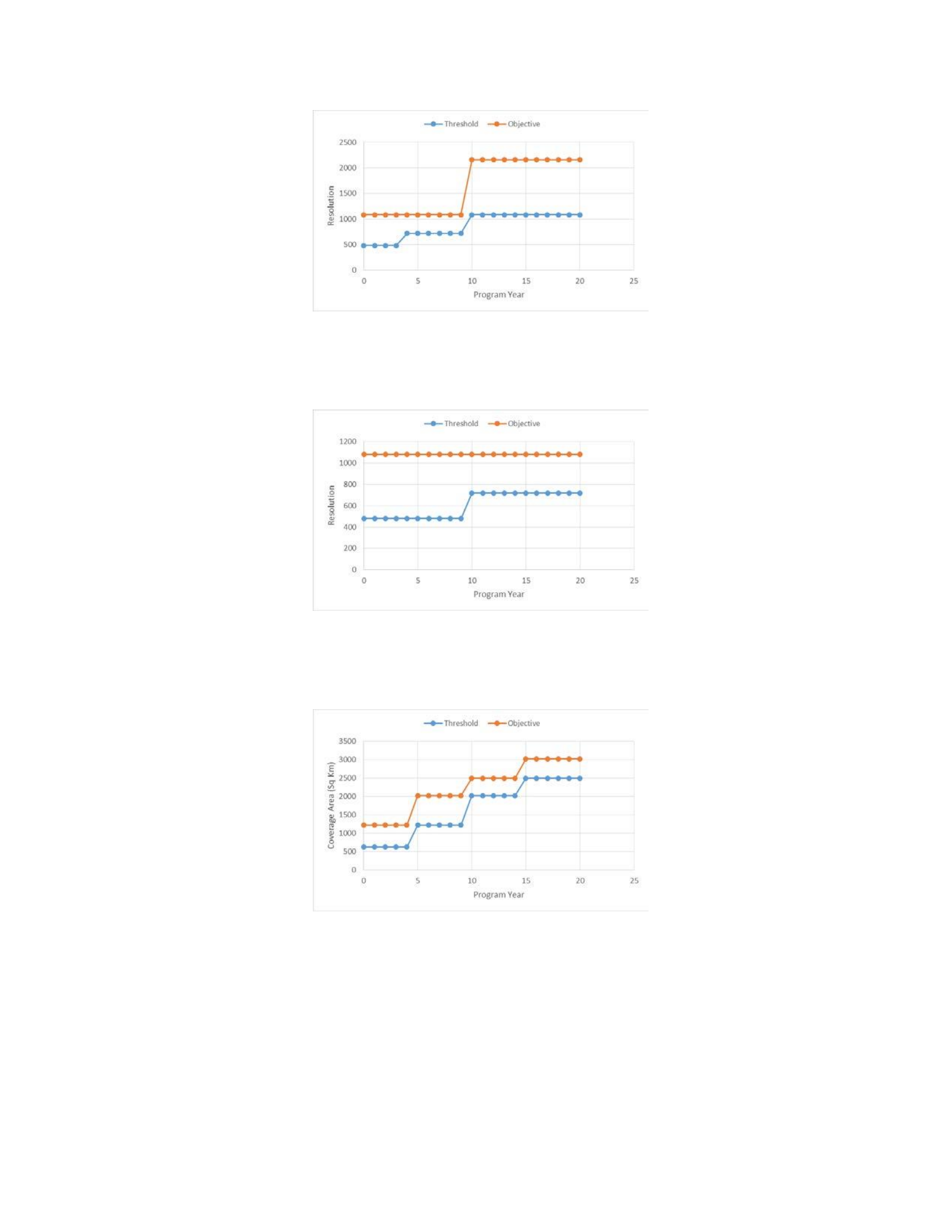
Figure 34: EO Video Resolution LURP

Figure 35: IR Video Resolution LURP

Figure 36: MTI Detection Coverage LURP

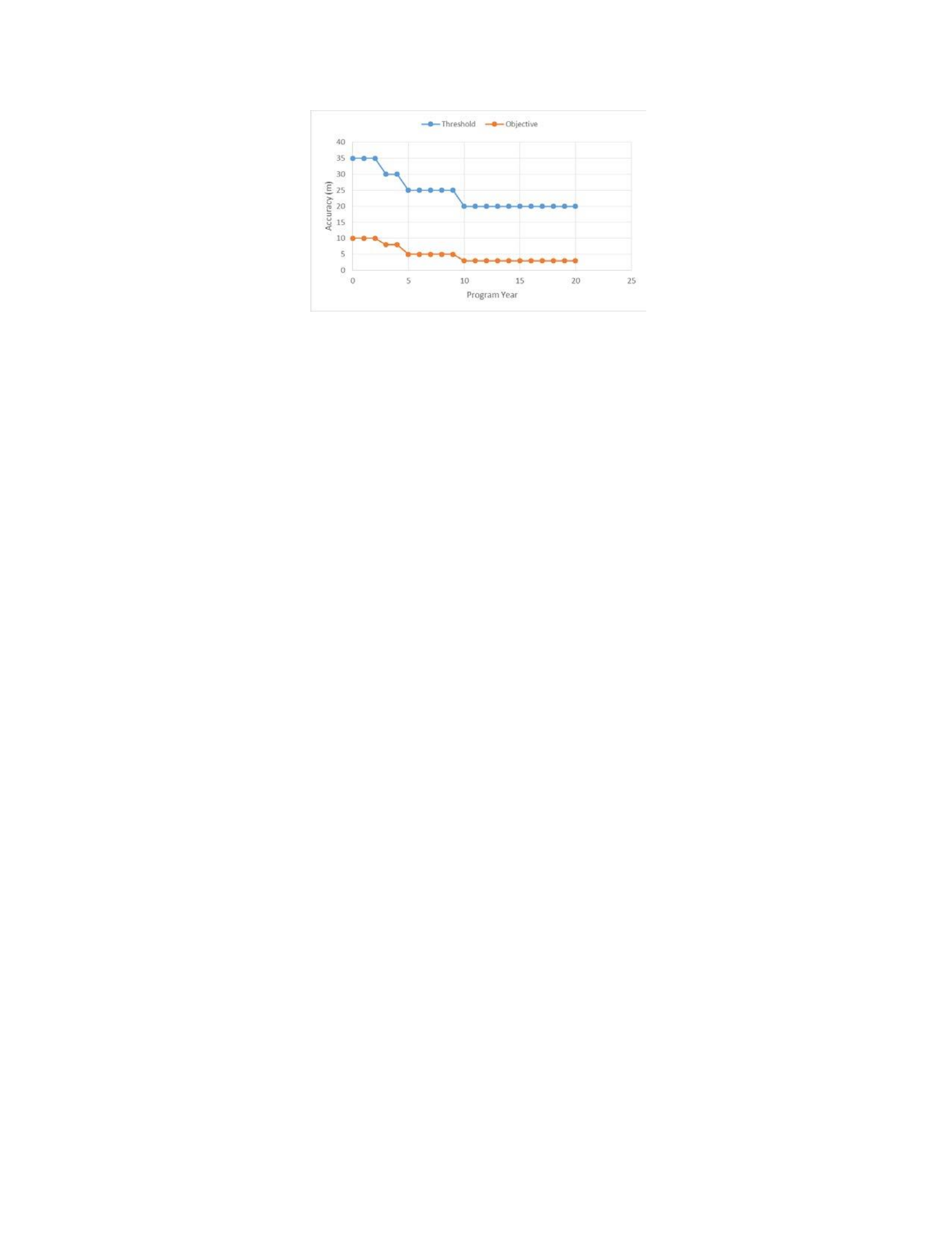
Figure 37: Subsystem A Geolocation Accuracy LURP The discontinuous

attributes for Program X achieved utility by either accomplishing the target value (with

threshold and objective the same value), or not. If they achieved the capability, then they

received maximum utility. If they did not provide the required capability, then they

received no utility. For example, if the MTI tracking algorithm produced radar tracks,

then the alternative received 100 utility for the Radar Tracking attribute. If the MTI

tracking algorithm wasn’t present in the alternative, then the alternative received 0

utility.

Step 2: Develop Program Reference Architecture

To provide the capabilities described above, Program X decided to procure a

medium sized commercial aircraft capable of hosting multiple sensors, processing

equipment and three analysts. The three analysts will be responsible for controlling all

payloads and performing limited analysis to support the Program X missions.

The program team also determined that Program X will require multiple key

subsystems, including:

• Full Motion Video subsystem

• Radar subsystem

• Subsystem A

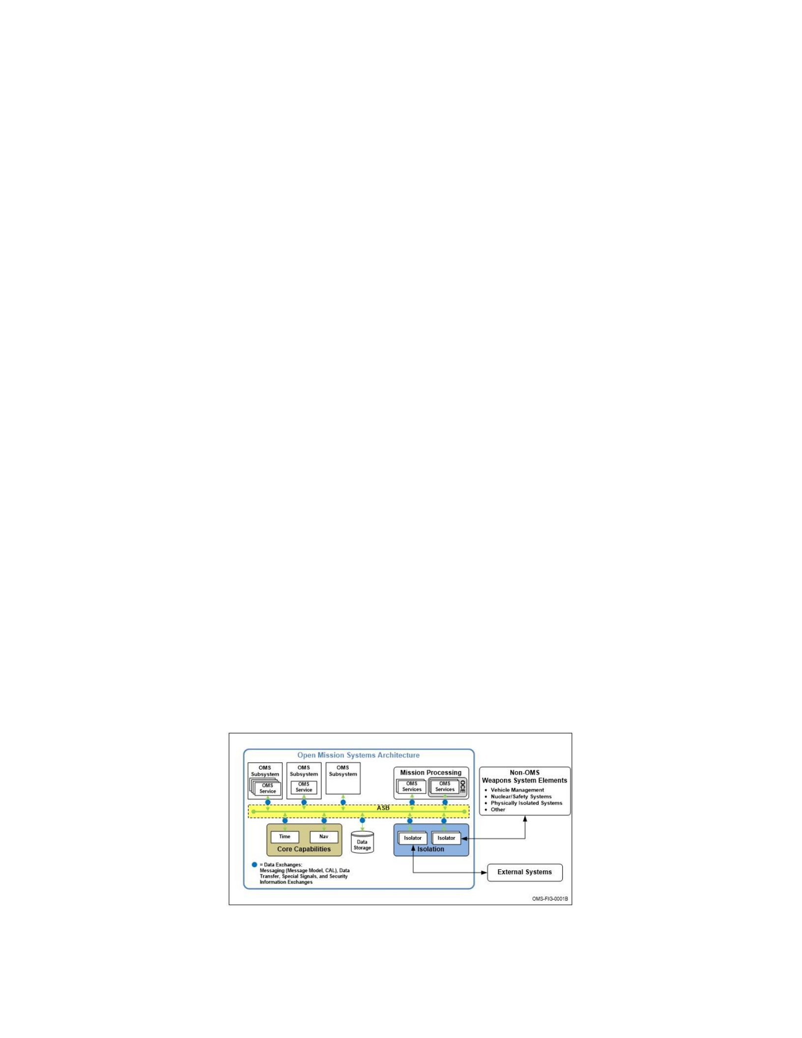
• Communications subsystem

• Three analyst workstations

Additionally, the system must integrate with the existing avionics system on the

host aircraft and use the SATCOM system to connect with terrestrial reach-back

networks. To accomplish this reach-back, the system will use the Open Mission Systems

(OMS) architecture standard.

The OMS requirements define several key interfaces and other architecture

practices. The detailed and complete OMS requirements can be found in the OMS

Definition and Documentation (OMS CWG, 2015). Among other requirements, OMS

defines all software interfaces between Services and Subsystems. OMS does this

primarily through the addition of a system component: the Avionics Service Bus (ASB).

The ASB is the software transport mechanism for OMS, supporting the movement of

command and control (C2) messages, products, streaming data, and special signals,

among other transport requirements. The messages utilized are the Unmanned Aircraft

Systems (UAS) Command and Control Initiatives (UCI) messages, while streaming data

and special signals conform to industry standards. Products are transported by a

combination of vendor-defined technology as well as commercial and government

standards.

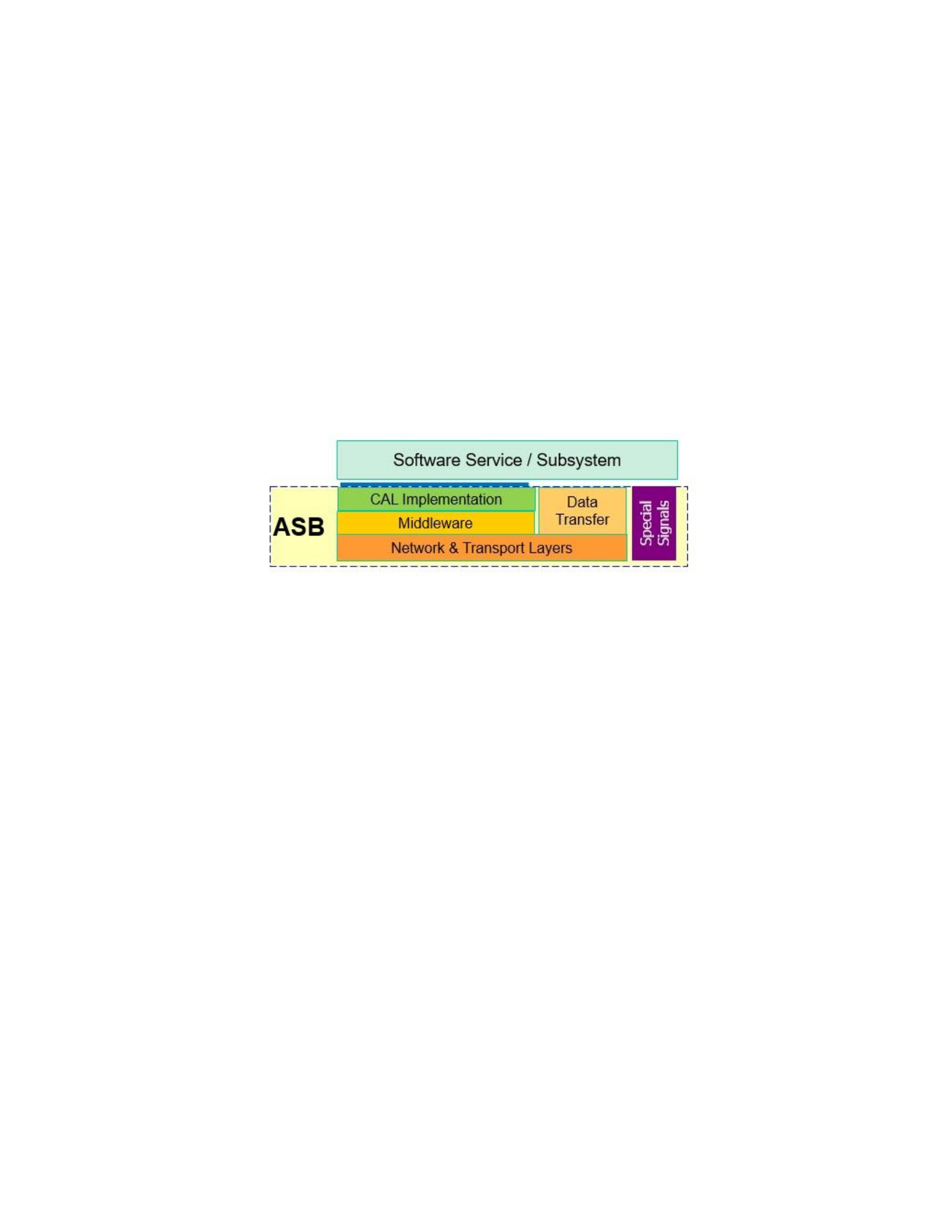
Figure 38: OMS Example Architecture (OMS CWG, 2015)

The ASB uses the Critical Abstraction Layer (CAL) to abstract the front end API

of the ASB from the transport capabilities themselves. To ensure interoperability, OMS

requires adherence to the CAL Application Program Interface (API) requirements. This

means that Subsystems and Services must utilize the CAL API for sending UCI messages

as well applicable Data Transfer standards. In some cases, this will require software to

adapt the Subsystem or Service native interfaces to OMS compliant interfaces and to

conform to the CAL API.

Figure 39: OMS Avionics Service Bus Diagram (OMS CWG, 2015)

OMS considers both Subsystems and Services to be “black boxes” meaning that

OMS does not define how the Subsystem or Service behaves inside its boundary. Instead,

the program can define additional requirements for behavior inside the Subsystem or

Service boundary according to the program business objectives. OMS also has the

concept of an Isolator, which is a component that provides specific isolation behavior

between the OMS mission package and the non-OMS systems.

Compliance in OMS is assessed in 3 tiers. Tier 1 requires adherence to the basic,

and most important, requirements of OMS. This includes (but is not limited to)

architecture definition practices, use of the ASB and CAL, non-proprietary

documentation, and the use of UCI messages. Tier 2 adds requirements, leading to Tier 3

which maximizes the benefits of OMS. It is important to note that both Tier 1 and Tier 2

allow non-OMS interactions between components, which still must be documented in a

non-proprietary manner. Tier 3 requires all interactions external to a Subsystem or

Service to comply with OMS requirements.

Program X has established the following OMS related architectural requirements:

• The system shall be an open system, incorporating a service oriented

architecture that utilizes non-proprietary government, commercial, and/or

industry interfaces and standards. The architecture shall include a Tier-3

compliant OMS Mission Package in accordance with the Open Mission

Systems (OMS) Definition and Documentation (D&D) V1.1. A Tier-3

compliant Mission Package will include a Tier-3 compliant OMS

Platform. The architecture will be layered or decoupled and

flexible/scalable to enable affordable, efficient, competitive capability

upgrades and technical refresh with minimum flight or mission software

re-write and regression testing. The processing hardware architecture will

integrate off-the-shelf technology to facilitate processing and memory

technical refresh to address product obsolescence.

• The FMV, Radar, Subsystem A and Communications capabilities shall be

Tier-3 compliant Subsystems in accordance with the Open Mission

Systems (OMS) Definition and Documentation (D&D) V1.1.

• The Analyst Workstation Network shall be composed of Tier 3 compliant

Services in accordance with the Open Mission Systems (OMS) Definition

and Documentation (D&D) V1.1.

These requirements are shown pictorially in the following reference architecture

diagram (Figure 38):

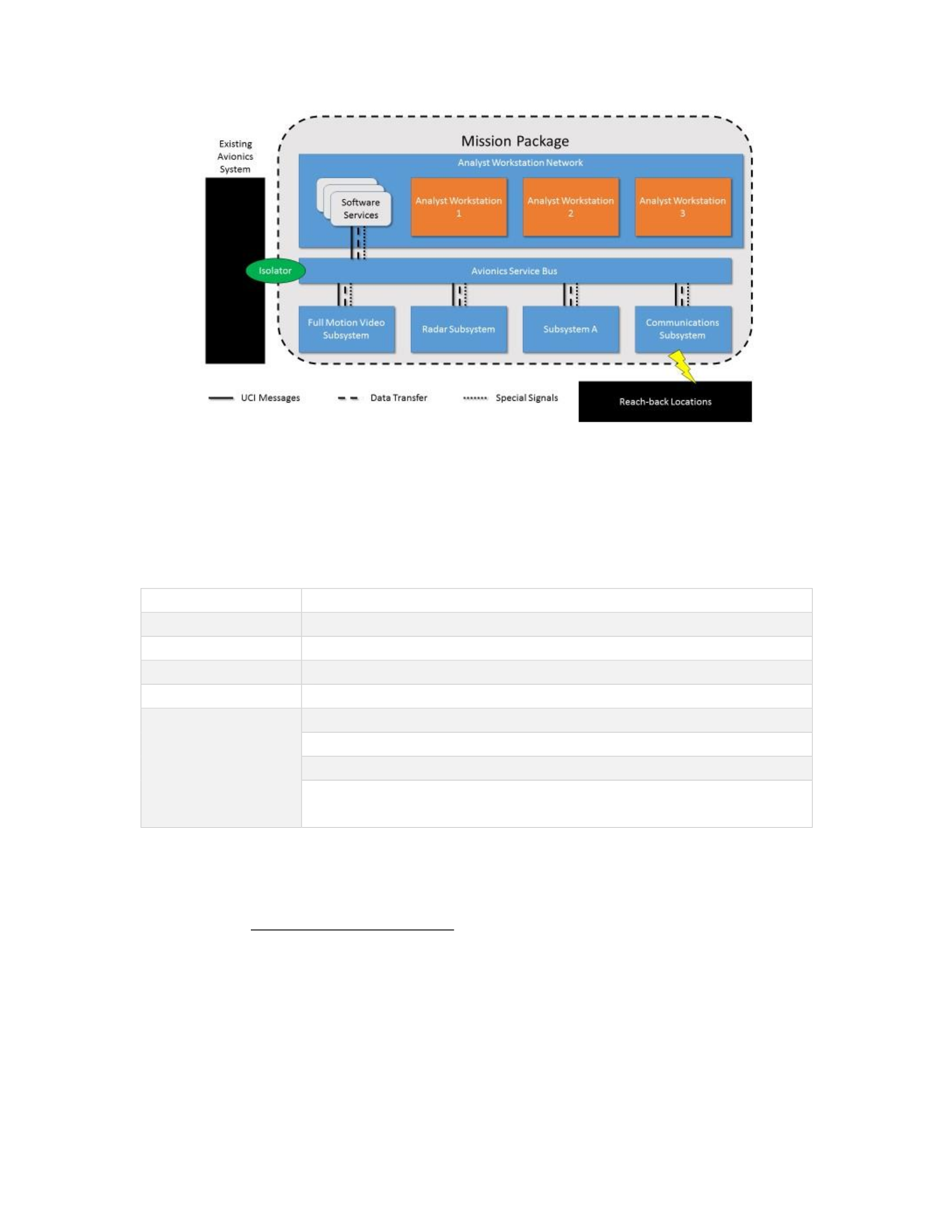
Figure 40: Program X Reference Architecture Diagram

In addition to OMS requirements, Program X chose to provide additional data

interface details for the initial design, as shown in the following table:

Table 9: Program X Additional Data Requirements

Logical Interface

Requirement

EO Video Data

H.264 compressed 1080p

IR Video Data

H.264 compressed 720p

MTI Detections

UCI Entity Message

Subsystem A

UCI Message (specified)

Map Data

JPEG 2000 compressed Imagery

Keyhole Markup Language

Shapefiles

JPEG 2000 compressed National Imagery Transfer File 2.1

reference imagery

Step 3: Create Alternatives

Prime Alternative

Initial Capability (Block 0)

The Prime Alternative was designed to take maximum advantage of off-the-shelf

components. The program team performed a market survey and found available

commercial off-the-shelf (COTS) components for the FMV, Radar and Communications

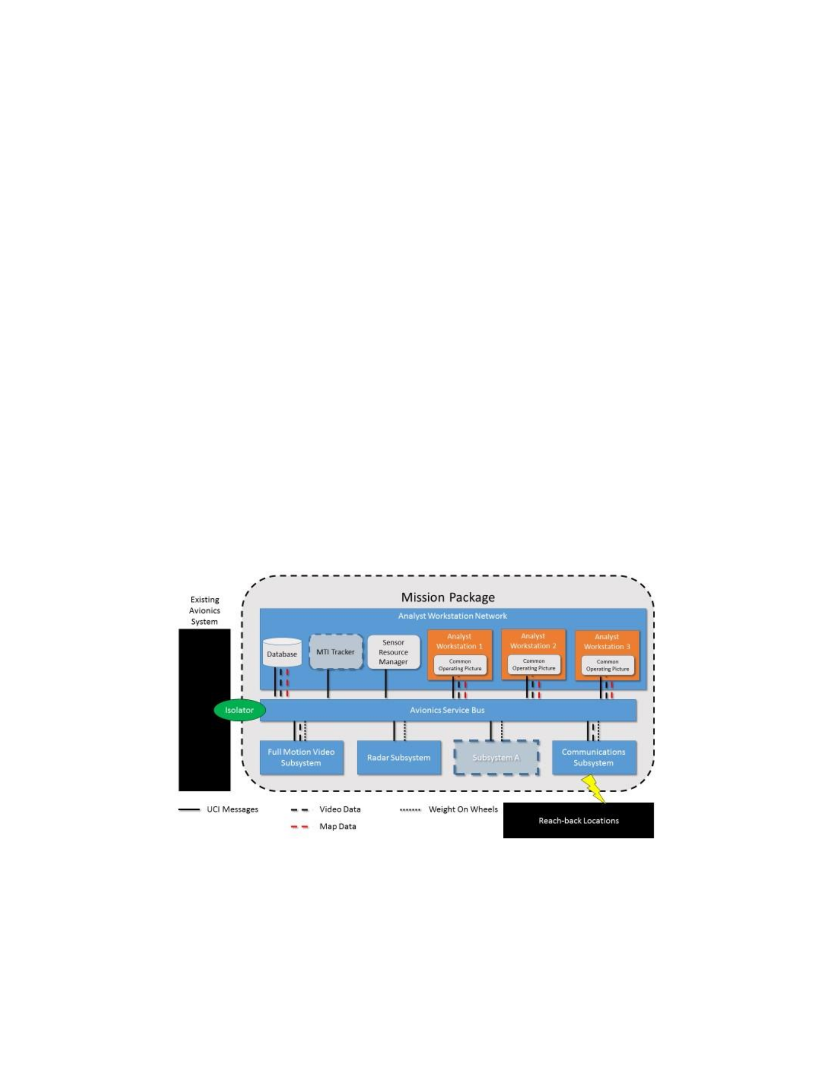
subsystem requirements. These systems meet the basic Program X capability

requirements and can be easily adapted to meet the reference architecture requirements.

No off the shelf components were found to meet the Subsystem A requirement, with the

earliest component becoming available in year 3 of the program. The ASB and Isolator

were found to be available commercially.

In addition to the subsystem requirements, the system must provide software for

the analyst workstations. The software, called the Common Operating Picture (COP) was

found to be immediately available off the shelf. Because each analyst must be able to

independently control and exploit data from any of the sensors, the system will require a

Sensor Resource Manager (SRM) to mediate sensor command and control and a common

database to store the data. Both of these components were identified as product lines

within the government. Finally, the MTI Tracker will be delivered as a government

product line, but will not be available until year 3.

Figure 41: Prime Alternative Architecture Implementation

All applicable subsystems will conform natively to the map and video standards,

including the FMV, ASB and Communications subsystems, as well as the COP

and database software. At program initiation, the only natively OMS/UCI

compliant capability will be the ASB. All other capabilities will require adapting

to OMS. Similarly, the Weight on Wheels (WoW) messages will require initial

modification for all installed capabilities. WoW messages communicate to the

various components of the system that the aircraft’s wheels are in contact with the

ground. This allows for certain functionality to be inhibited (such as radiation

from active sensors) to ensure safe operations.

The initial configuration will be able to be testing and delivery is anticipated

during year 2.

Block 10

Because the system will deploy without the MTI Tracker and Subsystem A, the

first modification will be intended to complete the Program X capabilities. Year 3 is the

anticipated completion timeframe for both systems, developed by their respective product

lines owners and ready for integration into the system. The addition of these two systems

will require updates to the COP, SRM and the database because the original software did

not include the basic capabilities. Both systems will require adaptation to OMS/UCI and

WoW.

Block 15

Block 15 will upgrade the Subsystem A subsystem in year 5 to respond to

changing mission requirements, as defined in the Subsystem A Geolocation Accuracy

LURP. The accuracy requirements increase in year 5, with the threshold moving from 30

to 25 meters, and the objective moving from 8 to 5 meters. This change will not require

changes to any other component, because the upgraded Subsystem A will conform to the

same interface standards as the previous version. Block 20

Block 20 will represent a major capability refresh of Program X in year 10,

featuring the upgrade of every primary sensor. The key upgrade will be the replacement

of the FMV sensor to handle 4K EO video and 1080p IR video. This upgrade will

respond to changing requirements that will see the threshold of the EO move from 720p

to 1080p, and the objective move from 1080p to 4K (aka 2160p). IR will have similar

changes, moving the threshold from 480p to 720p. The FMV upgrades will position both

sensors at maximum utility; if they are not upgraded, both would barely make the

threshold requirements. The new sensor will require adaptation to conform to OMS and

WoW requirements.

The upgrade in video resolution will have effects to the rest of the system. While

it would be possible to convert the video data to the existing 1080p/720p standard to

minimize the impacts to the system, this would have the effect of down-convert the video.

Down-convert, the process of converting a signal from a higher quality to a lower one,

would completely negate the improvements promised by the upgrade. Instead, the

Communications subsystem, COPs, and database will all be upgraded with systems that

natively support the increased resolution. While these systems will natively support the

improved resolution, they will need adaptation to OMS requirements.

In addition to the FMV upgrades, the Radar and Subsystem A subsystems will also

be upgraded. These subsystems will both require adaptation to OMS and WoW, but once

this is accomplished, there will be no other required changes to the rest of the system,

because the OMS interfaces will not change based on the upgrades.

Block 30

Block 30 will be an upgrade at year 15 with an upgraded Radar subsystem,

intended to increase the coverage of the MTI detection capability. This system will

require adaptation to OMS and WoW, but will not require any other changes to the

system.

Capabilities

For each of the upgrades, the Program X team predicted the expected capabilities

provided by the system (Table 10).

Table 10: Prime Alternative Expected Capabilities

Block 0

Block

10

Block

15

Block

20

Block

30

Delivery Year

2

3

5

10

15

KPP

EO Video Resolution

1080p

2160p

IR Video Resolution

720p

1080p

MTI Detection

Coverage

625 sq

km

625 sq

km

1300 sq

km

2100 sq

km

2500 sq

km

Disseminate FMV

Data

Yes

KSA

Radar Tracks

No

Yes

Disseminate MTI

Detections

Yes

Disseminate Radar

Tracks

No

Yes

Disseminate

Subsystem A Data

No

Yes

Subsystem A

Geolocation Accuracy

N/A

25m

10m

5m

Alternative 2

Alternative 2 will be very similar to the Prime Alternative, with the same systems

and basic architecture. However, instead of deploying the system early using available

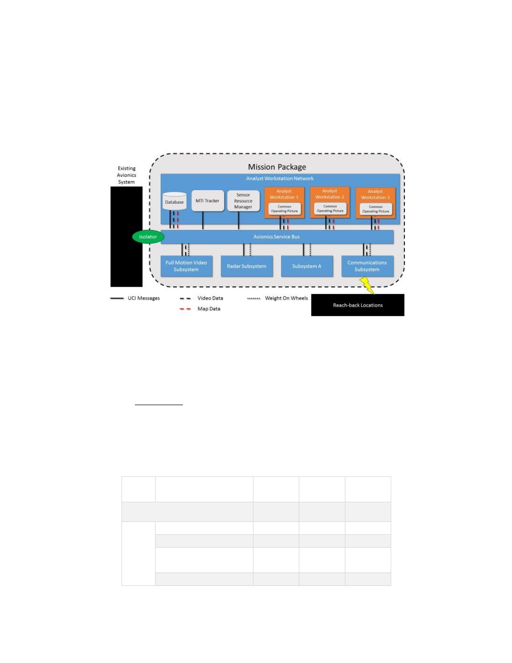
components, Alternative 2 delays system delivery until a fully capable system is ready.

This fully capable system will represent an identical solution to the system delivered by

the Prime Alternative after the Block 15 upgrades. In fact, the initial Alternative 2 system

will be delivered at the same time (year 5) as the Block 15 capable Prime Alternative.

Figure 42: Alternative 2 Architecture Implementation

From year 5 on, Alternative 2 will follow the same upgrade plan as the Prime

Alternative.

Capabilities

For each of the upgrades, the Program X team predicted the expected capabilities

provided by the system. This is shown in Table 11.

Table 11: Alternative 2 Expected Capabilities

Initial

Block

20

Block

30

Delivery Year

5

10

15

KPP

EO Video Resolution

1080p

2160p

IR Video Resolution

720p

1080p

MTI Detection

Coverage

1300 sq

km

2100 sq

km

2500 sq

km

Disseminate FMV

Yes

Data

KSA

Radar Tracks

Yes

Disseminate MTI

Detections

Yes

Disseminate Radar

Tracks

Yes

Disseminate

Subsystem A Data

Yes

Subsystem A

Geolocation Accuracy

10m

5m

Alternative 3

Alternative 3 will be a version of Alternative 2 that specifies additional key

interfaces within the Radar subsystem. In this alternative, the Radar subsystem will be

broken down into three major components:

• Processor. The Processor will send and receive C2 messaging with the

ASB, send RF C2 commands to the Receiver/Exciter, receive high level

RF Data from the Receiver/Exciter, process high level RF Data into MTI,

and send MTI detections to the ASB.

• Receiver/Exciter (REX). The REX will receive RF C2 commands from the

Processor, send low level RF C2 commands (aka RF pulses) to the Array,

receive low level RF Data (aka RF echoes) from the Array, amplifies

them, and send the amplified RF Data to the Processor.

• Array. The Array will receive low level RF C2 commands from the REX,

broadcast them, receive low level RF Data, and send this data to the REX.

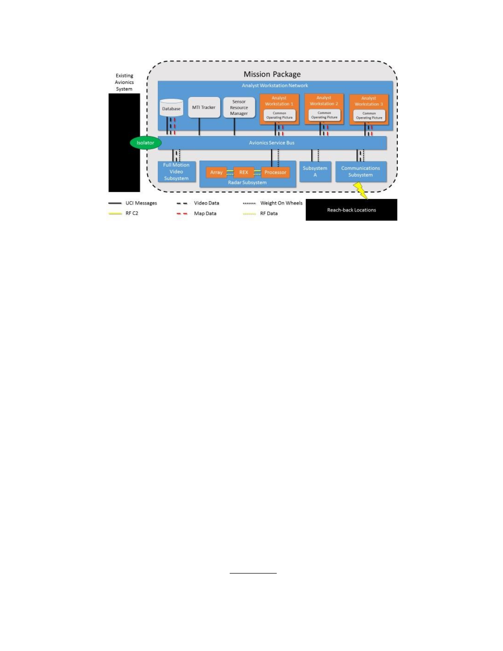
Figure 43: Alternative 3 Architecture Implementation

The system will be able to be tested and delivered during year 6, due to the

additional time and testing required to deploy the modular radar. The Processor will

require adaptation for OMS and WoW for the initial integration, but not for the remaining

Blocks. For the components, no modification will be needed at the interfaces because the

components will be designed for use together in the initial design.

For Blocks 20 and 30, all modifications except for the Radar will be identical to

Alternative 2. In Block 20, the REX will be upgraded to permit more power (and thus

more range), and the processor will be upgraded to account for this. The Array will be

unchanged. The Processor will require modification to handle the new RF C2 and RF

Data produced by the REX, and the REX will need to be modified to ensure

interoperability with the existing Array.

Block 30 will upgrade the Array to be more efficient using the power provided by

the previously upgraded REX, and the Processor will again be upgraded to take this into

account. These modifications will require modifying the Processor and Array to ensure

interoperability with the existing REX. Capabilities

For each of the upgrades, the Program X team predicted the expected capabilities

provided by the system (Table 12).

Table 12: Alternative 3 Expected Capabilities

Initial

Block

20

Block

30

Delivery Year

6

10

15

KPP

EO Video Resolution

1080p

2160p

IR Video Resolution

720p

1080p

MTI Detection

Coverage

1300 sq

km

2100 sq

km

2500 sq

km

Disseminate FMV

Data

Yes

KSA

Radar Tracks

Yes

Disseminate MTI

Detections

Yes

Disseminate Radar

Tracks

Yes

Disseminate

Subsystem A Data

Yes

Subsystem A

Geolocation Accuracy

10m

5m

Step 4: Compare Alternatives

Comparing the three alternatives required three primary efforts: calculating

operational utility, calculating cost, and calculating the CER. This section describes how

Program X performed each of these activities.

Operational Utility

Calculating the operational utility for each alternative was completed using the

methodology described in Chapter III. First, the incremental utility for each attribute was

found by applying its expected capability for a given year against the corresponding

annual utility curve found the in the attribute’s LURP. Next, the cumulative utility was

found by multiplying the incremental utility against the cumulative weight for the

attribute found in the Attribute Hierarchy. This calculation was performed every year for

each attribute. Table 13 shows an example of this, and Appendix A contains the

calculations for the remaining attributes.

Table 13: Prime Alternative Subsystem A Geolocation Accuracy Utility Calculations

Year

0

1

2

3

4

5

KSA Value (m)

N/A

25

10

Incremental

Utility

0

61.36364

87.5

Cumulative

Utility

0

6.724782

9.589041

Year

6

7

8

9

10

11

KSA Value (m)

10

5

Incremental

Utility

87.5

94.11765

Cumulative

Utility

9.589041

10.31426

Year

12

13

14

15

16

17

KSA Value (m)

5

Incremental

Utility

94.11765

Cumulative

Utility

10.31426

Year

18

19

20

Total

Avg

KSA Value (m)

5

N/A

Incremental

Utility

94.11765

1030.816

51.54078

Cumulative

Utility

10.31426

112.9661

5.648304

For example, to determine the cumulative utility for the Prime Alternative

Subsystem A Geolocation Accuracy for Year 5, the first step was to determine the

expected capability related to this attribute for Year 5. Using Table 10, the Subsystem A

Geolocation Accuracy for Year 5 was found to be 10 meters. Next, using the LURP for

Subsystem A Geolocation Accuracy (Figure 37), the incremental utility associated with

10 meter accuracy at Year 5 was 87.5. Finally, the incremental utility was multiplied by

the cumulative weight for Subsystem A Geolocation Accuracy (0.1096 from Figure 33).

This results in a cumulative utility for Subsystem A Geolocation Accuracy for Year 5 of

9.58.

Once the cumulative utility was found for all attributes for a given year, the

cumulative utilities were summed to create the operational utility for the alternative for

that year. Table 14 shows the operational utility for each alternative throughout the

lifecycle, as well as the average annual utility of each Alternative. Note that the Prime

Alternative produces approximately 15% more average utility than Alternative 2.

Table 14: Operational Utility Results

Year

0

1

2

3

4

5

Prime

0.00

62.87

86.58

89.88

Alternative 1

0.00

89.88

Alternative 2

0.00

Year

6

7

8

9

10

11

Prime

89.88

95.41

Alternative 1

89.88

95.41

Alternative 2

89.88

95.41

Year

12

13

14

15

16

17

Prime

95.41

94.67

Alternative 1

95.41

94.67

Alternative 2

95.41

94.67

Year

18

19

20

Total

Average

Prime

94.67

1730.48

86.52

Alternative 1

94.67

1494.46

74.72

Alternative 2

94.67

1404.58

70.23

The Prime Alternative showed utility early in the program life, compared to the

other alternatives which provided utility later. The additional area under the utility curve

translated to greater average utility across the lifecycle (Figure 42).

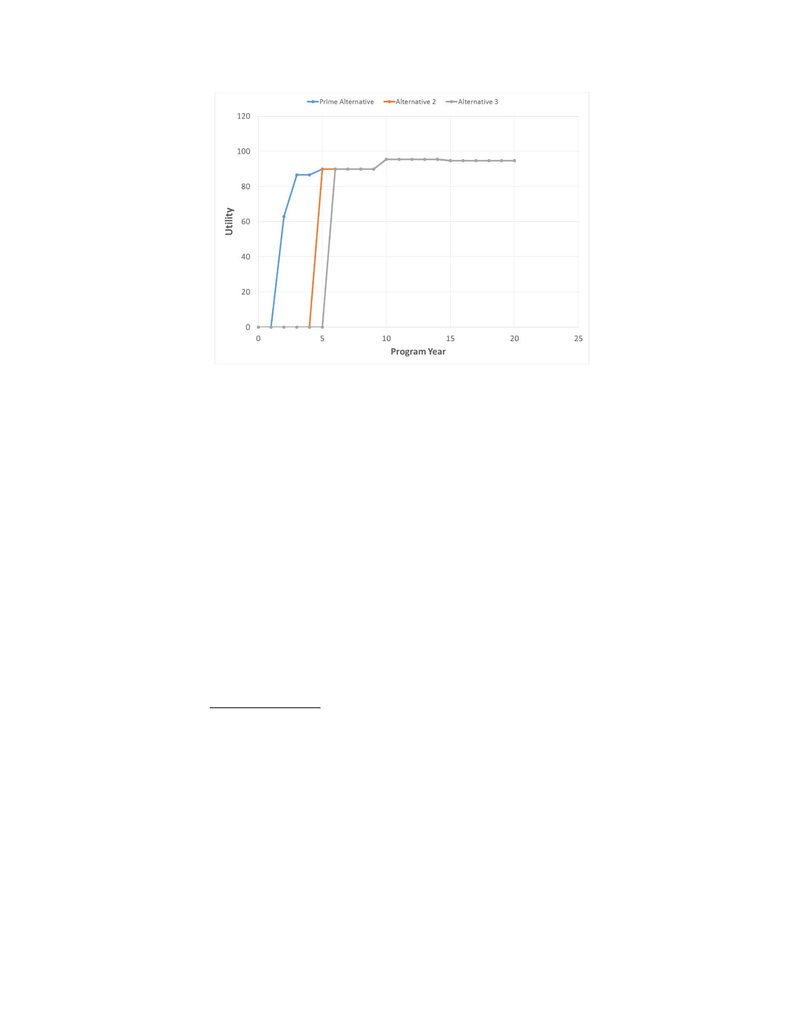
Figure 44: Comparison of Operational Utility over Time

Cost

Calculating cost was more complicated than calculating the utility of the

alternatives. Chapter III outlined the basic methodology, which is based around

evaluating the component acquisition and integration costs. This section will focus on

breaking down the CAC and CIC calculations for each alternative. This section does not

go show the detailed CIC calculations. Detailed discussion of the CIC (including the

COCOMO II details) is discussed in Appendix B.

Prime Alternative

Component Acquisition Cost

To calculate the CAC the reference cost for each component in the alternative was

determined. The reference costs for the Prime Alternative were found by identifying

offthe-shelf solutions and finding their actual costs. For the FMV, Radar, Subsystem A,

Analyst Workstations, and ASB, the numbers were available to Program X. However,

associating the numbers with a specific company was proprietary information in all cases.

As stated above, the MTI Tracker, SRM and Database were found within government

product lines and thus have zero reference cost. The reference costs are shown in Table

15.

Next, calibration factors are determined for each component in each block. For the

Prime Alternative, the factors were mostly 1, because the purchase cost for the

component was assumed to be the same as the reference cost. However, there were a

couple notable exceptions. For Block 15, the calibration factor for Subsystem A was 0.5,

meaning the purchase cost was 50% of the reference cost. This is because the system is

being modified, rather than completely replaced. In contrast, the calibration factors for the

FMV subsystem (cf = 1.4) and the Communications subsystem (cf = 2.0) were increased.

In the case of the FMV subsystem, the additional cost is due to the advanced sensor and

data processing. For the Communications subsystem, the additional cost is due to the

upgraded equipment necessary to send the additional FMV data through the SATCOM

system.

Table 15: Prime Alternative Component Acquisition Cost Calculations

Subsystem

Reference Cost

Block 0

Block 10

Block 15

cf

NRE

CAC

cf

NRE

CAC

cf

NRE

CAC

FMV

$

850,000.00

1

$ -

$

850,000.00

0

$ -

0

$ -

Radar

$

1,400,000.00

1

$ -

$

1,400,000.00

0

$ -

0

$ -

Subsystem A

$

200,000.00

0

$ -

1

$ -

$

200,000.00

0.5

$ -

$

100,000.00

Comms

$

850,000.00

1

$ -

$

850,000.00

0

$ -

0

$ -

Database

$ -

1

$ -

1

$

150,000.00

$

150,000.00

0

$ -

MTI Tracker

$ -

0

$ -

1

$ -

0

$ -

SRM

$ -

1

$ -

1

$ -

0

$ -

AW1

$

80,000.00

1

$ -

$

80,000.00

0

$ -

0

$ -

AW2

$

80,000.00

1

$ -

$

80,000.00

0

$ -

0

$ -

AW3

$

80,000.00

1

$ -

$

80,000.00

0

$ -

0

$ -

ASB

$

850,000.00

1

$ -

$

850,000.00

0

$ -

0

$ -

ASB

Reference Cost

Block 20

Block 30

cf

NRE

CAC

cf

NRE

CAC

FMV

$

850,000.00

1.4

$ -

$

1,190,000.00

0

$ -

Radar

$

1,400,000.00

1

$ -

$

1,400,000.00

1

$ -

$

1,400,000.00

Subsystem A

$

200,000.00

1

$ -

$

200,000.00

0

$ -

Comms

$

850,000.00

2

$ -

$

1,700,000.00

0

$ -

Database

$ -

1

$ -

0

$ -

MTI Tracker

$ -

0

$ -

0

$ -

SRM

$ -

0

$ -

0

$ -

AW1

$

80,000.00

1

$ -

$

80,000.00

0

$ -

AW2

$

80,000.00

1

$ -

$

80,000.00

0

$ -

AW3

$

80,000.00

1

$ -

$

80,000.00

0

$ -

ASB

$

850,000.00

0

$ -

0

$ -

The final piece of information required to calculate the CAC was the

NonRecurring Engineering (NRE) costs. As described in Chapter III, NRE costs represent

the investment that the program is required to make to modify, upgrade, or develop the

component. For the Prime Alternative, one system required NRE: the Database. This

component is provided by a government program office to Program X. However, the

Database program office did not budget for the modifications necessary to meet the

Program X Block 10 capability. Consequently, Program X will be required to fund the

modification. In all other cases, the product line owner will fund the modification and

make the new or upgraded component available to Program X.

Component Integration Cost

To calculate the CIC, the first step was to determine which interfaces require

modification for each component. The majority of required modifications for Program X

are due to the requirement to adapt a non-OMS compliant component to be able to

communicate with the ASB (Table 16), which will require adapting for sending and

receiving UCI messages (including software to comply with the CAL API), and

modification to use the OMS approved WoW special signal.

Table 16: Prime Alternative Modified Interfaces

Component

Interface Type

Endpoint

Block

0

10

15

20

30

FMV

UCI Messages

ASB

Yes

No

Yes

No

Video Data

ASB

No

WoW

ASB

Yes

No

Yes

No

Radar

UCI Messages

ASB

Yes

No

Yes

WoW

ASB

Yes

No

Yes

Subsystem A

UCI Messages

ASB

No

Yes

No

WoW

ASB

No

Yes

No

Comms

UCI Messages

ASB

Yes

No

Yes

No

Video Data

ASB

No

WoW

ASB

Yes

No

Yes

No

Database

UCI Messages

ASB

Yes

No

Yes

No

Video Data

ASB

No

Map Data

ASB

No

MTI Tracker

UCI Messages

ASB

No

Yes

No

SRM

UCI Messages

ASB

Yes

No

AW1

UCI Messages

ASB

Yes

No

Yes

No

Video Data

ASB

No

Map Data

ASB

No

AW2

UCI Messages

ASB

Yes

No

Yes

No

Video Data

ASB

No

Map Data

ASB

No

AW3

UCI Messages

ASB

Yes

No

Yes

No

Video Data

ASB

No

Map Data

ASB

No

ASB

Isolator

Legacy

Systems

Yes

No

Video data and map data will not require modification due to the use of widely

available standards, as described earlier in this chapter (Table 9). The only ASB interface

shown in Table 16 is the Isolator, because the ASB end of the ASB-to-Subsystem/Service

interfaces will be compliant with UCI messages, the Video Data, and Map Data standards

as a requirement of being OMS compliant.

Once the interfaces requiring modification were identified, the cost of each

interface modification was determined. For Program X, the estimated cost to create each

specific interface end was found using the COCOMO II equation (Center for Software

Engineering, 2000: 1). This process is described in detail in Appendix C, and the results

for the Prime Alternative CIC calculations are shown in Table 17.

Table 17: Prime Alternative Component Interface Cost Calculations

Component

Interface Type

Endpoint

Interface

Cost

Block

0

10

15

20

30

FMV

UCI Messages

ASB

$

68,247.41

$

68,247.41

$ -

$

68,247.41

$ -

Video Data

ASB

$

387,974.51

$ -

WoW

ASB

$

36,295.46

$

36,295.46

$ -

$

36,295.46

$ -

Radar

UCI Messages

ASB

$

68,247.41

$

68,247.41

$ -

$

68,247.41

$

68,247.41

WoW

ASB

$

36,295.46

$

36,295.46

$ -

$

36,295.46

$

36,295.46

Subsystem A

UCI Messages

ASB

$

68,247.41

$ -

$

68,247.41

$

68,247.41

$

68,247.41

$ -

WoW

ASB

$

36,295.46

$ -

$

36,295.46

$

36,295.46

$

36,295.46

$ -

Comms

UCI Messages

ASB

$

142,508.32

$

142,508.32

$ -

$

142,508.32

$ -

Video Data

ASB

$

60,919.76

$ -

WoW

ASB

$

36,295.46

$

36,295.46

$ -

$

36,295.46

$ -

Database

UCI Messages

ASB

$

124,121.13

$

124,121.13

$

124,121.13

$ -

$

124,121.13

$ -

Video Data

ASB

$

265,623.40

$ -

Map Data

ASB

$

51,718.67

$ -

MTI Tracker

UCI Messages

ASB

$

54,194.18

$ -

$

54,194.18

$ -

SRM

UCI Messages

ASB

$

73,563.53

$

73,563.53

$ -

AW1

UCI Messages

ASB

$

135,135.68

$

135,135.68

$

135,135.68

$ -

$

135,135.68

$ -

Video Data

ASB

$

156,342.81

$ -

Map Data

ASB

$

156,342.81

$ -

AW2

UCI Messages

ASB

$

135,135.68

$

135,135.68

$

135,135.68

$ -

$

135,135.68

$ -

Video Data

ASB

$

156,342.81

$ -

Map Data

ASB

$

156,342.81

$ -

AW3

UCI Messages

ASB

$

135,135.68

$

135,135.68

$

135,135.68

$ -

$

135,135.68

$ -

Video Data

ASB

$

156,342.81

$ -

Map Data

ASB

$

156,342.81

$ -

ASB

Isolator

Legacy

Systems

$

458,212.46

$

458,212.46

$ -

Total Cost

Once the CAC and CIC were calculated for each component in every design

increment, the total costs were found by summing the costs for each block (Table 18).

Table 18: Prime Alternative Total Cost Calculations

Block 0

Block 10

Block 15

Block 20

Block 30

Total

FMV

CAC

$

850,000.00

$ -

$

1,190,000.00

$ -

$

2,040,000.00

CIC

$

104,542.86

$ -

$

104,542.86

$ -

$

209,085.72

Total

$

954,542.86

$ -

$

1,294,542.86

$ -

$

2,249,085.72

Radar

CAC

$

1,400,000.00

$ -

$

1,400,000.00

$

1,400,000.00

$

4,200,000.00

CIC

$

104,542.86

$ -

$

104,542.86

$

104,542.86

$

313,628.59

Total

$

1,504,542.86

$ -

$

1,504,542.86

$

1,504,542.86

$

4,513,628.59

Subsystem

A

CAC

$ -

$

200,000.00

$

100,000.00

$

200,000.00

$ -

$

500,000.00

CIC

$ -

$

104,542.86

$

104,542.86

$

104,542.86

$ -

$

313,628.59

Total

$ -

$

304,542.86

$

204,542.86

$

304,542.86

$ -

$

813,628.59

Comms

CAC

$

850,000.00

$ -

$

1,700,000.00

$ -

$

2,550,000.00

CIC

$

178,803.77

$ -

$

178,803.77

$ -

$

357,607.55

Total

$

1,028,803.77

$ -

$

1,878,803.77

$ -

$

2,907,607.55

Database

CAC

$ -

$

150,000.00

$ -

$

150,000.00

CIC

$

124,121.13

$

124,121.13

$ -

$

124,121.13

$ -

$

372,363.39

Total

$

124,121.13

$

274,121.13

$ -

$

124,121.13

$ -

$

522,363.39

CAC

$ -

MTI

Tracker

CIC

$ -

$

54,194.18

$ -

$

54,194.18

Total

$ -

$

54,194.18

$ -

$

54,194.18

SRM

CAC

$ -

CIC

$

73,563.53

$ -

$

73,563.53

Total

$

73,563.53

$ -

$

73,563.53

AW1

CAC

$

80,000.00

$ -

$

80,000.00

$ -

$

160,000.00

CIC

$

135,135.68

$

135,135.68

$ -

$

135,135.68

$ -

$

405,407.04

Total

$

215,135.68

$

135,135.68

$ -

$

215,135.68

$ -

$

565,407.04

AW2

CAC

$

80,000.00

$ -

$

80,000.00

$ -

$

160,000.00

CIC

$

135,135.68

$

135,135.68

$ -

$

135,135.68

$ -

$

405,407.04

Total

$

215,135.68

$

135,135.68

$ -

$

215,135.68

$ -

$

565,407.04

AW3

CAC

$

80,000.00

$ -

$

80,000.00

$ -

$

160,000.00

CIC

$

135,135.68

$

135,135.68

$ -

$

135,135.68

$ -

$

405,407.04

Total

$

215,135.68

$

135,135.68

$ -

$

215,135.68

$ -

$

565,407.04

ASB

CAC

$

850,000.00

$ -

$

850,000.00

CIC

$

458,212.46

$ -

$

458,212.46

Total

$

1,308,212.46

$ -

$

1,308,212.46

Total

$

11,278,387.32

$ 2,076,530.42

$ 409,085.72

$

11,503,921.05

$ 3,009,085.72

$

28,277,010.24

Alternative 2

The cost calculations for Alternative 2 were very similar to the Prime Alternative.

The CAC calculations used the same factors for Blocks 20 and 30, while Block 0

combined factors from Blocks 0, 10 and 15 of the Prime Alternative (Table 19).

Alternative 2 also will have virtually identical component interfaces to the Prime

Alternative (Table 20). The Alternative 2 CIC calculations followed the same

methodology used by the Prime Alternative (Table 21). The CAC and CIC were then used

to calculate the total cost (Table 22).

Table 19: Alternative 2 Component Acquisition Cost Calculations

Subsystem

Reference Cost

Block 0

Block 20

Block 30

cf

NRE

CAC

cf

NRE

CAC

cf

NRE

CAC

FMV

$

850,000.00

1

$ -

$

850,000.00

1.4

$ -

$ 1,190,000.00

0

$ -

Radar

$

1,400,000.00

1

$ -

$

1,400,000.00

1

$ -

$ 1,400,000.00

1

$ -

$

1,400,000.00

Subsystem A

$

200,000.00

1

$ -

$

200,000.00

1

$ -

$

200,000.00

0

$ -

Comms

$

850,000.00

1

$ -

$

850,000.00

2

$ -

$ 1,700,000.00

0

$ -

Database

$ -

1

$ -

1

$ -

0

$ -

MTI Tracker

$ -

0

$ -

0

$ -

0

$ -

SRM

$ -

1

$ -

0

$ -

0

$ -

AW1

$

80,000.00

1

$ -

$

80,000.00

1

$ -

$

80,000.00

0

$ -

AW2

$

80,000.00

1

$ -

$

80,000.00

1

$ -

$

80,000.00

0

$ -

AW3

$

80,000.00

1

$ -

$

80,000.00

1

$ -

$

80,000.00

0

$ -

ASB

$

850,000.00

1

$ -

$

850,000.00

0

$ -

0

$ -

Table 20: Alternative 2 Modified Component Interfaces

Component

Interface Type

Endpoint

Block

0

20

30

FMV

UCI Messages

ASB

Yes

No

Video Data

ASB

No

WoW

ASB

Yes

No

Radar

UCI Messages

ASB

Yes

WoW

ASB

Yes

Subsystem A

UCI Messages

ASB

Yes

No

WoW

ASB

Yes

No

Comms

UCI Messages

ASB

Yes

No

Video Data

ASB

No

WoW

ASB

Yes

No

Database

UCI Messages

ASB

Yes

No

Video Data

ASB

No

Map Data

ASB

No

MTI Tracker

UCI Messages

ASB

No

SRM

UCI Messages

ASB

Yes

No

AW1

UCI Messages

ASB

Yes

No

Video Data

ASB

No

Map Data

ASB

No

AW2

UCI Messages

ASB

Yes

No

Video Data

ASB

No

Map Data

ASB

No

AW3

UCI Messages

ASB

Yes

No

Video Data

ASB

No

Map Data

ASB

No

ASB

Isolator

Legacy

Systems

Yes

No

Table 21: Alternative 2 Component Interface Cost Calculations

Component

Interface Type

Endpoint

Interface Cost

Block

0

20

30

FMV

UCI Messages

ASB

$

68,247.41

$

68,247.41

$

68,247.41

$ -

Video Data

ASB

$

387,974.51

$ -

WoW

ASB

$

36,295.46

$

36,295.46

$

36,295.46

$ -

Radar

UCI Messages

ASB

$

68,247.41

$

68,247.41

$

68,247.41

$

68,247.41

WoW

ASB

$

36,295.46

$

36,295.46

$

36,295.46

$

36,295.46

Subsystem A

UCI Messages

ASB

$

68,247.41

$

68,247.41

$

68,247.41

$ -

WoW

ASB

$

36,295.46

$

36,295.46

$

36,295.46

$ -

Comms

UCI Messages

ASB

$

142,508.32

$

142,508.32

$

142,508.32

$ -

Video Data

ASB

$

60,919.76

$ -

WoW

ASB

$

36,295.46

$

36,295.46

$

36,295.46

$ -

Database

UCI Messages

ASB

$

124,121.13

$

124,121.13

$

124,121.13

$ -

Video Data

ASB

$

265,623.40

$ -

Map Data

ASB

$

51,718.67

$ -

MTI Tracker

UCI Messages

ASB

$

54,194.18

$ -

SRM

UCI Messages

ASB

$

73,563.53

$

73,563.53

$ -

AW1

UCI Messages

ASB

$

135,135.68

$

135,135.68

$

135,135.68

$ -

Video Data

ASB

$

156,342.81

$ -

Map Data

ASB

$

156,342.81

$ -

AW2

UCI Messages

ASB

$

135,135.68

$

135,135.68

$

135,135.68

$ -

Video Data

ASB

$

156,342.81

$ -

Map Data

ASB

$

156,342.81

$ -

AW3

UCI Messages

ASB

$

135,135.68

$

135,135.68

$

135,135.68

$ -

Video Data

ASB

$

156,342.81

$ -

Map Data

ASB

$

156,342.81

$ -

ASB

Isolator

Legacy

Systems

$

458,212.46

$

458,212.46

$ -

Table 22: Alternative 2 Total Cost Calculations

Block 0

Block 20

Block 30

Total

FMV

CAC

$

850,000.00

$ 1,190,000.00

$ -

$

2,040,000.00

CIC

$

104,542.86

$

104,542.86

$ -

$

209,085.72

Total

$

954,542.86

$ 1,294,542.86

$ -

$

2,249,085.72

Radar

CAC

$ 1,400,000.00

$

1,400,000.00

$

4,200,000.00

CIC

$

104,542.86

$

104,542.86

$

104,542.86

$

313,628.59

Total

$ 1,504,542.86

$

1,504,542.86

$

4,513,628.59

Subsystem

A

CAC

$

200,000.00

$

200,000.00

$ -

$

400,000.00

CIC

$

104,542.86

$

104,542.86

$ -

$

209,085.72

Total

$

304,542.86

$

304,542.86

$ -

$

609,085.72

Comms

CAC

$

850,000.00

$ 1,700,000.00

$ -

$

2,550,000.00

CIC

$

178,803.77

$

178,803.77

$ -

$

357,607.55

Total

$ 1,028,803.77

$ 1,878,803.77

$ -

$

2,907,607.55

Database

CAC

$ -

CIC

$

124,121.13

$

124,121.13

$ -

$

248,242.26

Total

$

124,121.13

$

124,121.13

$ -

$

248,242.26

MTI Tracker

CAC

$ -

CIC

$ -

Total

$ -

SRM

CAC

$ -

CIC

$

73,563.53

$ -

$

73,563.53

Total

$

73,563.53

$ -

$

73,563.53

AW1

CAC

$

80,000.00

$

80,000.00

$ -

$

160,000.00

CIC

$

135,135.68

$

135,135.68

$ -

$

270,271.36

Total

$

215,135.68

$

215,135.68

$ -

$

430,271.36

AW2

CAC

$

80,000.00

$

80,000.00

$ -

$

160,000.00

CIC

$

135,135.68

$

135,135.68

$ -

$

270,271.36

Total

$

215,135.68

$

215,135.68

$ -

$

430,271.36

AW3

CAC

$

80,000.00

$

80,000.00

$ -

$

160,000.00

CIC

$

135,135.68

$

135,135.68

$ -

$

270,271.36

Total

$

215,135.68

$

215,135.68

$ -

$

430,271.36

ASB

CAC

$

850,000.00

$ -

$

850,000.00

CIC

$

458,212.46

$ -

$

458,212.46

Total

$

1,308,212.46

$ -

$

1,308,212.46

Total

$ 11,887,473.04

$ 11,503,921.05

$ 3,009,085.72

$

26,400,479.82

Alternative 3

The cost calculations for Alternative 3 were more complicated than Alternative 2

because Alternative 3 splits the Radar subsystem into three components: the Radar

Processor, REX, and Array. For the CAC, the reference costs of these new components

were determined using engineering judgment and are notional for this analysis because

similar systems in this class don’t currently exist. Reference costs for non-Radar

components were unchanged from Alternative 2. The CAC calculations are shown in

Table 23.

Table 23: Alternative 3 Component Acquisition Cost Calculations

Subsystem

Reference

Cost

Block 0

Block 20

Block 30

cf

NRE

CAC

cf

NRE

CAC

cf

NRE

CAC

FMV

$

850,000.00

1

$ -

$

850,000.00

1.4

$ -

$

1,190,000.00

0

$ -

Radar - Processor

$

300,000.00

1

$ -

$

300,000.00

0.3

$

400,000.00

$

475,000.00

0.3

$

500,000.00

$

575,000.00

Radar - REX

$

500,000.00

1

$ -

$

500,000.00

1

$ -

$

500,000.00

0

$ -

Radar - Array

$

200,000.00

1

$

400,000.00

$

600,000.00

0

$ -

1

$

400,000.00

$

600,000.00

Subsystem A

$

200,000.00

1

$ -

$

200,000.00

1

$ -

$

200,000.00

0

$ -

Comms

$

850,000.00

1

$ -

$

850,000.00

2

$ -

$

1,700,000.00

0

$ -

Database

$ -

1

$ -

1

$ -

0

$ -

MTI Tracker

$ -

0

$ -

0

$ -

0

$ -

SRM

$ -

1

$ -

0

$ -

0

$ -

AW1

$

80,000.00

1

$ -

$

80,000.00

1

$ -

$

80,000.00

0

$ -

AW2

$

80,000.00

1

$ -

$

80,000.00

1

$ -

$

80,000.00

0

$ -

AW3

$

80,000.00

1

$ -

$

80,000.00

1

$ -

$

80,000.00

0

$ -

ASB

$

850,000.00

1

$ -

$

850,000.00

0

$ -

0

$ -

For Block 20, the calibration factor for the Processor was 0.3, representing a cost

reduction to modify the components, while the REX will be entirely replaced at full

reference cost (cf = 1.0). The Array will not modified in Block 20, so no cost was

incurred. For Block 30, the Processor will again be modified (cf = 0.3), the Array will be

replaced (cf = 1.0) and the REX remains unmodified. Calibration factors for non-Radar

components were unchanged from the other alternatives.

In terms of NRE, it was assumed that the initial Processor and REX will be

available OTS, while the Array will need to be tailored for the specific application of

Program X. This means that the Array will need to be modified to function at Program

X’s airspeed, altitude, power levels, etc… Because these modifications will be specific to

Program X, the program will be required to fund the NRE. For Block 20, the Processor

will be modified, but the modifications will be Program X specific, requiring NRE

expenditure. For Block 30, both the Processor and Array will require Program X specific

modifications, and thus NRE expenditure. The amount of NRE was estimated using

engineering judgment.

The modifications required to support the Radar upgrades performed in Blocks 20

and 30 have been described as part of the general description of Alternative 3 above.

Table 24 shows which interfaces will be modified in each design increment, while Table

25 shows the CIC calculations for Alternative 3. Finally, Table 26 shows the total cost

calculations for Alternative 3.

Table 24: Alternative 3 Modified Component Interfaces

Component

Interface Type

Endpoint

Block

0

20

30

FMV

UCI Messages

ASB

Yes

No

Video Data

ASB

No

WoW

ASB

Yes

No

Radar -

Processor

UCI Messages

ASB

Yes

No

WoW

ASB

Yes

No

RF C2

REX

No

Yes

RF Data

REX

No

Yes

Radar - REX

RF C2

Processor

No

RF Data

Processor

No

RF C2

Array

No

Yes

No

RF Data

Array

No

Yes

No

Radar - Array

RF C2

REX

No

Yes

RF Data

REX

No

Yes

Subsystem A

UCI Messages

ASB

Yes

No

WoW

ASB

Yes

No

Comms

UCI Messages

ASB

Yes

No

Video Data

ASB

No

WoW

ASB

Yes

No

Database

UCI Messages

ASB

Yes

No

Video Data

ASB

No

Map Data

ASB

No

MTI Tracker

UCI Messages

ASB

No

SRM

UCI Messages

ASB

Yes

No

AW1

UCI Messages

ASB

Yes

No

Video Data

ASB

No

Map Data

ASB

No

AW2

UCI Messages

ASB

Yes

No

Video Data

ASB

No

Map Data

ASB

No

AW3

UCI Messages

ASB

Yes

No

Video Data

ASB

No

Map Data

ASB

No

ASB

Isolator

Legacy

Systems

Yes

No

Table 25: Alternative 3 Component Interface Calculations

Component

Interface Type

Endpoint

Interface

Cost

Block

0

20

30

FMV

UCI Messages

ASB

$

68,247.41

$

68,247.41

$

68,247.41

$ -

Video Data

ASB

$

387,974.51

$ -

WoW

ASB

$

36,295.46

$

36,295.46

$

36,295.46

$ -

Radar -

Processor

UCI Messages

ASB

$

68,247.41

$

68,247.41

$ -

WoW

ASB

$

36,295.46

$

36,295.46

$ -

RF C2

REX

$ -

RF Data

REX

$

110,527.17

$ -

$

110,527.17

$

110,527.17

Radar - REX

RF C2

Processor

$

110,527.17

$ -

RF Data

Processor

$

96,767.68

$ -

RF C2

Array

$

110,527.17

$ -

$

110,527.17

$ -

RF Data

Array

$

96,767.68

$ -

$

96,767.68

$ -

Radar - Array

RF C2

REX

$

110,527.17

$ -

$

110,527.17

RF Data

REX

$

96,767.68

$ -

$

96,767.68

Subsystem A

UCI Messages

ASB

$

68,247.41

$

68,247.41

$

68,247.41

$ -

WoW

ASB

$

36,295.46

$

36,295.46

$

36,295.46

$ -

Comms

UCI Messages

ASB

$

142,508.32

$

142,508.32

$

142,508.32

$ -

Video Data

ASB

$

60,919.76

$ -

WoW

ASB

$

36,295.46

$

36,295.46

$

36,295.46

$ -

Database

UCI Messages

ASB

$

124,121.13

$

124,121.13

$

124,121.13

$ -

Video Data

ASB

$

265,623.40

$ -

Map Data

ASB

$

51,718.67

$ -

MTI Tracker

UCI Messages

ASB

$

54,194.18

$ -

SRM

UCI Messages

ASB

$

73,563.53

$

73,563.53

$ -

AW1

UCI Messages

ASB

$

135,135.68

$

135,135.68

$

135,135.68

$ -

Video Data

ASB

$

156,342.81

$ -

Map Data

ASB

$

156,342.81

$ -

AW2

UCI Messages

ASB

$

135,135.68

$

135,135.68

$

135,135.68

$ -

Video Data

ASB

$

156,342.81

$ -

Map Data

ASB

$

156,342.81

$ -

AW3

UCI Messages

ASB

$

135,135.68

$

135,135.68

$

135,135.68

$ -

Video Data

ASB

$

156,342.81

$ -

Map Data

ASB

$

156,342.81

$ -

ASB

Isolator

Legacy

Systems

$

458,212.46

$

458,212.46

$ -

Table 26: Alternative 3 Total Cost Calculations

Block 0

Block 20

Block 30

Total

FMV

CAC

$

850,000.00

$

1,190,000.00

$ -

$

2,040,000.00

CIC

$

104,542.86

$

104,542.86

$ -

$

209,085.72

Total

$

954,542.86

$

1,294,542.86

$ -

$

2,249,085.72

Radar -

Processor

CAC

$

300,000.00

$

475,000.00

$

575,000.00

$

1,350,000.00

CIC

$

104,542.86

$ -

$

104,542.86

Total

$

404,542.86

$

475,000.00

$

575,000.00

$

1,454,542.86

Radar - REX

CAC

$

500,000.00

$

500,000.00

$ -

$

1,000,000.00

CIC

$ -

$

207,294.86

$ -

$

207,294.86

Total

$

500,000.00

$

707,294.86

$ -

$

1,207,294.86

Radar -

Array

CAC

$

600,000.00

$ -

$

600,000.00

$

1,200,000.00

CIC

$ -

$

207,294.86

$

207,294.86

Total

$

600,000.00

$ -

$

807,294.86

$

1,407,294.86

Subsystem

A

CAC

$

200,000.00

$

200,000.00

$ -

$

400,000.00

CIC

$

104,542.86

$

104,542.86

$ -

$

209,085.72

Total

$

304,542.86

$

304,542.86

$ -

$

609,085.72

Comms

CAC

$

850,000.00

$

1,700,000.00

$ -

$

2,550,000.00

CIC

$

178,803.77

$

178,803.77

$ -

$

357,607.55

Total

$

1,028,803.77

$

1,878,803.77

$ -

$

2,907,607.55

Database

CAC

$ -

CIC

$

124,121.13

$

124,121.13

$ -

$

248,242.26

Total

$

124,121.13

$

124,121.13

$ -

$

248,242.26

MTI

Tracker

CAC

$ -

CIC

$ -

Total

$ -

SRM

CAC

$ -

CIC

$

73,563.53

$ -

$

73,563.53

Total

$

73,563.53

$ -

$

73,563.53

AW1

CAC

$

80,000.00

$

80,000.00

$ -

$

160,000.00

CIC

$

135,135.68

$

135,135.68

$ -

$

270,271.36

Total

$

215,135.68

$

215,135.68

$ -

$

430,271.36

AW2

CAC

$

80,000.00

$

80,000.00

$ -

$

160,000.00

CIC

$

135,135.68

$

135,135.68

$ -

$

270,271.36

Total

$

215,135.68

$

215,135.68

$ -

$

430,271.36

AW3

CAC

$

80,000.00

$

80,000.00

$ -

$

160,000.00

CIC

$

135,135.68

$

135,135.68

$ -

$

270,271.36

Total

$

215,135.68

$

215,135.68

$ -

$

430,271.36

ASB

CAC

$

850,000.00

$ -

$

850,000.00

CIC

$

458,212.46

$ -

$

458,212.46

Total

$

1,308,212.46

$ -

$

1,308,212.46

Total

$ 11,887,473.04

$ 10,859,425.04

$ 2,764,589.71

$ 25,511,487.80

Cost Comparison

Direct comparison of the alternatives showed that the Prime Alternative was the

most expensive Alternative, with a cost of $28.3M. Alternative 2 was the second most

expensive, at $26.4M. Finally, Alternative 3 was the least expensive, at $25.5M. The

Prime Alternative was the most costly due to its five design increments, compared to only

three for Alternatives 2 and 3. Alternative 3 was the least costly because the entire Radar

will not be modified in Blocks 20 and 30; in contrast, the other alternatives intend to

replace the entire Radar each time. Evaluating only on cost, the cost differences between

the alternatives are significant, with the Prime Alternative requiring 11% more funds than

Alternative 3. However, considering only cost ignores the utility of the capability. To

account for the delivered utility, the ACEF calculates cost effectiveness. Cost

Effectiveness

Using only utility or cost to compare the Program X alternatives would result in

different preferences:

• Highest utility: Prime Alternative

• Lowest cost alternative: Alternative 3

Because of this, additional comparisons of the cost effectiveness were required to

select an alternative. As described in Chapter III, the first cost effectiveness comparison

in ACEF was the Instantaneous Cost Effectiveness Ratio (ICER). Figure 43 shows the

comparison of ICER across the lifecycle of Program X.

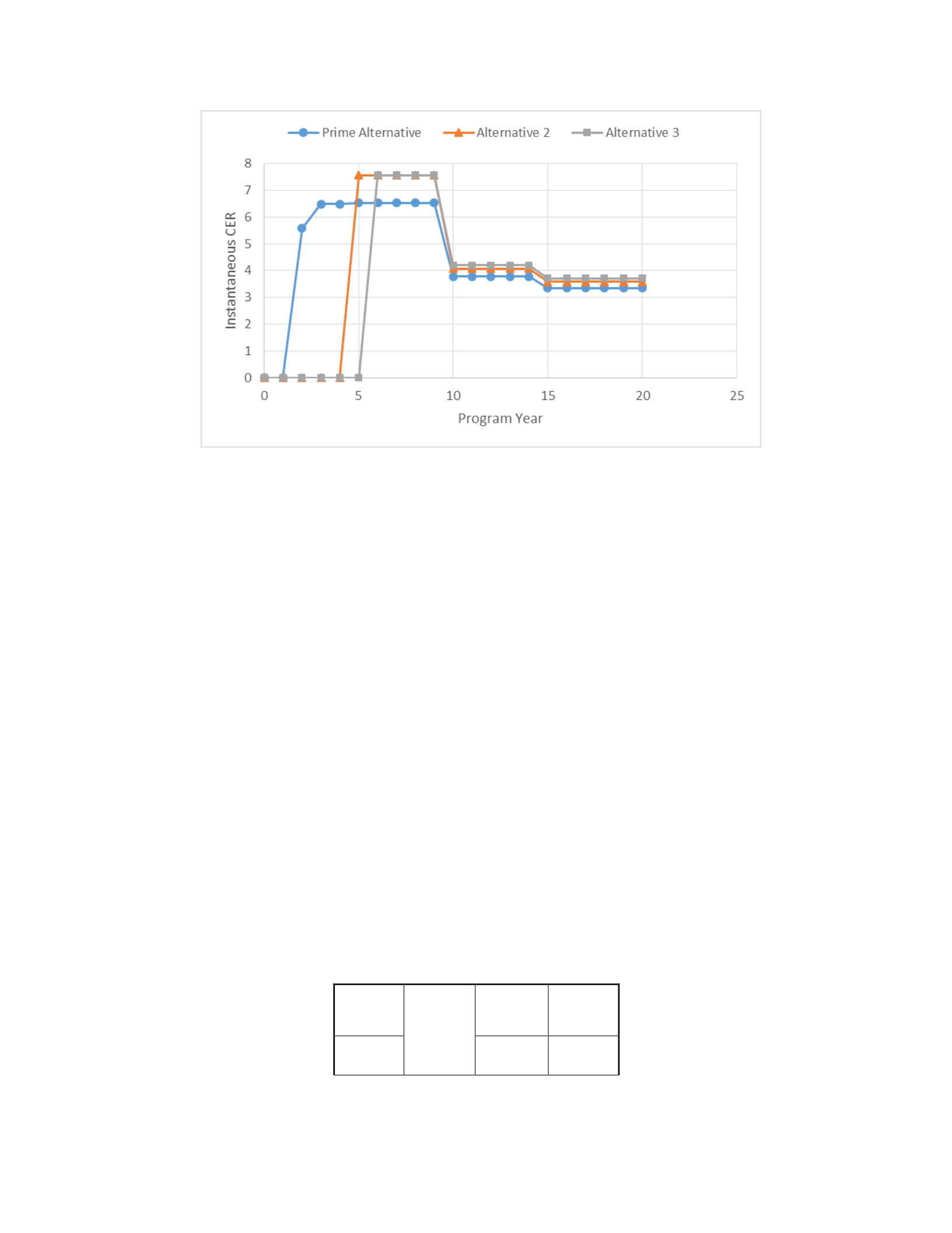
Figure 45: Instantaneous Cost Effectiveness Ratio Comparison

As this figure shows, the Prime Alternative demonstrated high ICER early in the

lifecycle. This was expected, because the Prime Alternative will deliver capability 3 years

prior to Alternative 2 and 4 years prior to Alternative 2. However, after Year 5 the Prime

Alternative demonstrated lower ICER than the alternatives. Between Year 5 and Year 10,

Alternatives 2 and 3 had equal ICER. However, after Year 10 Alternative 3 began to have

the highest ICER. The reduced cost for Blocks 20 and 30 were due to the modular Radar

subsystem.

Because no one alternative had the highest ICER throughout the lifecycle, it was

difficult to use the ICER to determine the overall most cost effective alternative.

Consequently, Program X used the lifecycle cost effectiveness ratio (LCER) described in

Chapter III (Table 27).

Table 27: Lifecycle Cost Effectiveness Ratio Calculations

Average

Annual

Operational

Utility

Lifecycle Cost

Cost

Effectiveness

Ratio

($M)

(Utility per year

per $M)

Prime

86.52

$28.28

3.06

Alternative 1

74.72

$26.40

2.83

Alternative 2

70.23

$25.51

2.75

The ACEF analysis showed that despite having the highest lifecycle cost, the

Prime Alternative produced the highest LCER. This meant that for a given dollar, the

Prime Alternative produced more operational utility per year than either other alternative.

Alternative 3 produced the least LCER. This was likely because Alternative 3 takes an

extra year to deploy the initial design increment. This “lost opportunity” to deliver

operational utility offset the reduced cost for the two modification blocks.

Step 5: Account for Uncertainty

Cumulative Weight Sensitivity Analysis

As part of the ACEF analysis, Program X conducted a sensitivity analysis to vary

the cumulative weights. The original importance ratings were varied individually. As they

were varied, the rest of the weights on the branch were adjusted to keep the original

proportion between the remaining ratings. Ratings on the other branch were unmodified.

In addition, the branch level ratings were also varied. High and low ratings were created

for all attributes, excluding the EO Video Resolution and Subsystem A Geolocation

Accuracy, which were already at maximum importance rating. After these ratings were

created, the analysis was re-run for each of the alternatives. Table 28, Table 29, and Table

30 show the analysis.

Table 28: Prime Alternative Sensitivity Analysis

Low

Rating

LCER

High

Rating

Low

Nominal

High

KPP

0.2

3.0855918

3.034155615

0.8

KPPs

EO Video Resolution

80

3.04071832

N/A

IR Video Resolution

60

3.06353325

3.056214165

100

MTI Detection Coverage

25

3.12750631

2.992241107

75

Disseminate Video Data

80

3.05071243

3.069034981

100

KSAs

Radar Tracks

60

3.05858895

3.059873708

3.061158469

100

Disseminate MTI Detections

40

3.05403524

3.065712178

80

Disseminate Radar Tracks

25

3.05280731

3.066940111

75

Disseminate System A Data

65

3.0592424

3.061136318

95

System A Geolocation Accuracy

80

3.0694071

N/A

Table 29: Alternative 2 Sensitivity Analysis

Low

Rating

LCER

High

Rating

Low

Nominal

High

KPP

0.2

2.87498826

2.785732916

0.8

KPPs

EO Video Resolution

80

2.81458917

N/A

IR Video Resolution

60

2.83010774

2.830613438

100

MTI Detection Coverage

25

2.89185134

2.768869842

75

Disseminate Video Data

80

2.82281774

2.837903443

100

KSAs

Radar Tracks

60

2.82850784

2.83036059

2.832213343

100

Disseminate MTI Detections

40

2.82862933

2.832091851

80

Disseminate Radar Tracks

25

2.82826521

2.832455966

75

Disseminate System A Data

65

2.82945019

2.832181399

95

System A Geolocation Accuracy

80

2.83564094

N/A

Table 30: Alternative 3 Sensitivity Analysis

Low

Rating

LCER

High

Rating

Low

Nominal

High

KPP

0.2

2.79463948

2.711019282

0.8

KPPs

EO Video Resolution

80

2.73806704

N/A

IR Video Resolution

60

2.75105664

2.754602115

100

MTI Detection Coverage

25

2.81311663

2.692542131

75

Disseminate Video Data

80

2.74576913

2.759889628

100

KSAs

Radar Tracks

60

2.75110047

2.75282938

2.754558289

100

Disseminate MTI Detections

40

2.75121384

2.754444918

80

Disseminate Radar Tracks

25

2.75087407

2.754784693

75

Disseminate System A Data

65

2.75197983

2.75452848

95

System A Geolocation Accuracy

80

2.75775677

N/A

The sensitivity analysis showed that all three alternatives had little sensitivity to

large changes in cumulative weight. Varying the branch level weights did not have the

greatest effect on the results. For all three alternatives, varying the MTI Detection

Coverage resulted in the largest deltas, with +/- 2.2% each. Varying the KPP had a delta

of +/- 0.8% for the Prime Alternative and +/- 1.5% for the other two alternatives. In

contrast, no other attribute had a delta over +/- 0.26%. The MTI Detection Coverage

likely had the highest deltas because it had the lowest utility values throughout the

lifecycle. Reducing the weight of the MTI Detection Coverage actually increased the

LCER, because it reduced the impact of the low utility scores from the underperforming

Radar subsystem. The other weights have limited impact because they represent

capabilities that largely exhibit maximum utility throughout the lifecycle (Table 31).

Table 31: Prime Alternative Average Utility per Attribute

KPPs

EO Video Resolution

95

IR Video Resolution

83

MTI Detection Coverage

50.64556

Disseminate FMV Data

95

KSAs

Radar Tracks

90

Disseminate MTI Detections

95

Disseminate Radar Tracks

95

Disseminate System A Data

90

System A Geolocation Accuracy

79.77607

The MTI Detection Coverage averaged 50% utility throughout the lifecycle means

that it can have a disproportionate effect on the overall operational utility, and thus the

LCER. The remaining attributes had high average utility and “desensitized” the system,

resulting in low overall sensitivity to changing cumulative weights. Additionally, the

behavior of each alternative was similar because the later blocks produce identical

capabilities.

Lifecycle Utility Reference Profile Sensitivity Analysis

In addition to varying the cumulative weights, the LURPs should be varied. For

this analysis, the EO Video Resolution LURP was varied (Figure 44). Other LURPs were

omitted for brevity, but could be varied using the same technique.

Scenario 1 represented accelerated EO Video Resolution requirements, starting

with a 1080p objective, and building to 4K (current technical limit), and growing to 8K.

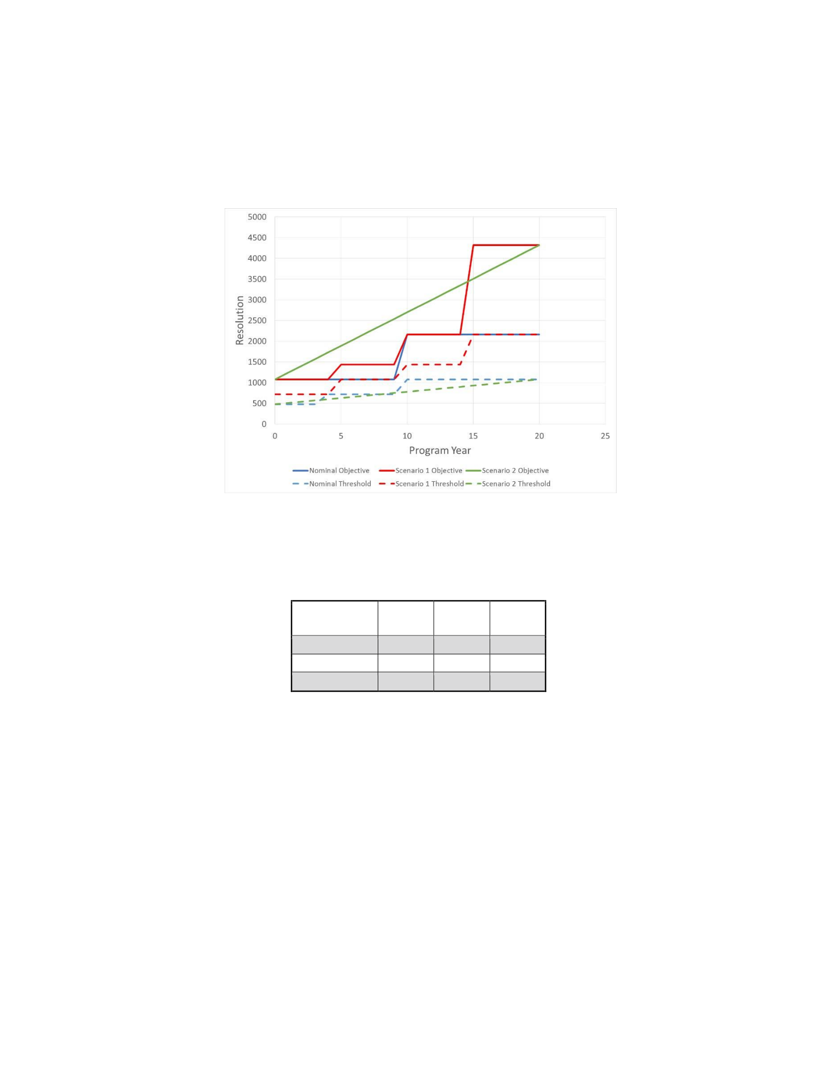
8K cameras were very limited at the time of the analysis, so 8K was considered a stretch

objective. Scenario 2 represented a different approach: a very wide trade space that

changes linearly throughout the lifecycle (Figure 44).

Figure 46: EO Video Resolution LURP Scenarios The

analysis was re-run for each of these scenarios (Table 32).

Table 32: EO Video Resolution Sensitivity Analysis Results

Nominal

Scenario 1

Scenario 2

Prime Alternative

3.06

2.88

Alternative 1

2.83

2.64

2.67

Alternative 2

2.75

2.57

2.60

Table 32 shows that the LCER was sensitive to the LURPs, with quite large

changes to each alternative from the nominal scenario to the two alternative scenarios.

This was due to the addition of 8K video objective requirements that did not exist in the

nominal LURP. However, this did not largely affect the difference between the

alternatives. The Prime Alternative still maintains 0.22 utility per $M per year advantage

over Alternative 1. This small difference is most likely because all three alternatives will

acquire the same FMV subsystem to produce the same capabilities. For alternatives that

used dissimilar subsystems, the large changes between the scenarios may result in more

important changes in LCER.

Step 6: Examine Results and Update Business Strategy

The results of the Program X ACEF analysis showed that the Prime Alternative

experienced the highest lifecycle cost effectiveness, even in the face of changing user

preference and changing requirements. This analysis shows that producing operational

utility early produced the highest lifecycle cost effectiveness. Even though the Prime

Alternative did not achieve the highest ICER at any time other than when the other

alternatives weren’t deployed, it still produced the highest LCER. This is shown in Figure

44, where the Prime Alternative displays a rapid delivery of ICER, which then levels out.

The area under the ICER curve for the Prime Alternative is larger than the other

alternatives, translating to larger LCER.

However, the open radar subsystem showed promise, even though Alternative 3

did not exploit its full potential. For the next round of analysis, Program X should

investigate alternatives similar to the Prime Alternative, but including more use of the

open radar subsystem. For example, an additional alternative would deploy a system with

FMV only, integrating the open radar when it became available. Another potential is to

deploy with an OTS radar, replacing it with an open radar when it becomes available. As

part of this process, the program should investigate methods to take advantage of this

open capability. One example to consider is the ARCI program; Program X could use a

similar process to have annual/biannual software upgrades to the Radar Processor to

incrementally increase the radar capability and build operational utility earlier in the

lifecycle.

Additionally, this analysis showed that the Business Strategy should be updated.

The mix of KPPs and KSAs was not optimal, because only a relative few attributes ended

up contributing to differences between the alternatives in the analysis. In the next round

of analysis, Program X should consider limiting the number of KPPs and KSAs that don’t

discriminate between alternatives. For example, combining all communications related

capabilities that have binary utility values into a single roll up value. Additionally, the

program should consider adding additional APAs that may assist discrimination between

alternatives.

Investigation Questions

The Investigation Questions necessary to address the research question were laid

out in Chapter I. This section restates the questions and provides explicit answers.

Investigation Question 1

How are operational requirements defined and communicated? Operational

requirements are defined according to the JCIDS process, and communicated through the

use of KPPs and KSAs. This was discussed in Chapter II, and used as a basis for

calculating utility in ACEF.

Investigation Question 2

What is MOSA, and how are programs applying it? MOSA was described in

Chapter II, along with a detailed discussion of how programs are applying it. In summary,

programs are applying MOSA inconsistently as identified by multiple sources discussed

in Chapter II. Researching this question led to the ACEF approach by identifying the need

for consistent methods for evaluating cost effectiveness.

Investigation Question 3

How can cost effectiveness be estimated throughout the program lifecycle? This

research proposes the ACEF to estimate cost effectiveness throughout the program

lifecycle.

Investigation Question 4

How can operational utility be measured throughout the program lifecycle? In

ACEF, operational utility is measured against the program operational requirements as

defined using existing requirements documents (i.e ICD, CDD, CPD). MAUA is used to

aggregate the operational utility as measured against each requirement into a single

operational utility value. In addition, LURPs are used to evaluate operational utility in the

face of changing requirements.

Investigation Question 5

How can the cost of MOSA be measured throughout the program lifecycle? In

ACEF, the MOSA costs are estimated by evaluating the cost to acquire and integrate

components. This was described in detail in Chapter III and an example was shown in

Chapter IV.

Summary

Chapter IV focuses on demonstrating the ACEF using a notional ISR program

called Program X. First, a Business Strategy was established for Program X. This

included an Attribute Hierarchy and set of LURPs. A program reference architecture was

developed, followed by a set of alternatives. These alternatives were evaluated in terms of

both operational utility and cost throughout the lifecycle, and both instantaneous and

lifecycle cost effectiveness ratios were calculated. Using the basic scenario, two

sensitivity analyses were performed, including one for the cumulative weights and one

for a LURP. The ACEF analysis was completed by analyzing the results, which were used

to update both the Reference Architecture and Business Strategy. Finally, the

Investigation Questions presented in Chapter I were re-visited and answered.

V. Conclusions and Recommendations

Chapter Overview

This chapter describes the development of the ACEF, and relates the significance

of the research to DoD programs. This chapter also describes recommendations for action

to begin implementing ACEF and recommendations for further research to improve the

ACEF. This chapter, and this research, ends with conclusions on the ACEF approach.

Significance of Research

The use of MOSA has not achieved the desired effects of reduced cost and

schedule for acquisition programs. At least part of this reason is that programs either do

not include appropriate MOSA attributes in their design, or allow them to be traded away

for other requirements (Kendall, 2015). The ACEF is designed to assist DoD program

managers by allowing them to understand how differing architecture alternatives deliver

operational utility at a given cost. This analysis facilitates traceability between the

specific architecture requirements and operational utility. This knowledge will allow the

program manager to prioritize the architectural requirements and then defend priorities

over time. This knowledge may result in better realization of the benefits expected of

MOSA application

Recommendations for Action

Standardize Methods for Value-Focused Requirements

ACEF would be greatly assisted by improvements to how program teams think of

operational capability requirements. Identifying program tradespace to develop creative

solutions that maximize value while clearly establishing consistent methods for defining

that value, will result in lower cost and faster delivery. The tradespace can take the form

of the LURPs described in ACEF or other methods; the key is to find methods to

incentivize programs to develop innovative solutions. Standardizing this concept will

involve allowing programs to deliver partial solution, requiring stakeholder commitment

to incremental delivery in line with DoD policy. Standardization will also require

developing tools and training to enable the DoD to implement the changes.

Collect Data on Modifications

Regardless of whether ACEF is utilized, the DoD must collect data on the cost to

modify systems. This data must be of sufficient technical detail to identify the specific

activities that drive costs. Among the data that must be collected:

• Identification of affected interface

• Cost to modify interfaces

• Identification of affected components

• Cost to modify components

• Cost to procure modified components

• Additional unexpected costs

The costs from multiple programs should be collected by a common team and

examined to identify trends and improve estimation techniques. These updated techniques

will be used to improve the ACEF.

Develop Tools and Training for ACEF

To ensure that the benefits made possible by this research are achieved, tools and

training should be developed to support application of the ACEF methodology. The

development of analytical software tools that can be run on DoD networks and be

provided to contract analysts will significantly reduce the burden for applying the

methodology. These tools should focus on ensuring that the analysts work through the

process logically, with assisted business strategy and reference architecture development,

standardized cost and utility generations methods, and by automatically generating

standardized graphical and statistical outputs. Additionally, training must be developed

that is intuitive for non-specialists, so analyses can be run rapidly by the target user base:

government decision-makers.

Recommendations for Future Research

Support for Non-Software Interfaces

This analysis did not support non-software interfaces such as hardware or

mechanical interfaces. Future research should investigate how to integrate non-software

interfaces into the ACEF. The basic procedure of ACEF is generic enough to account for

any type of interface, but the specific execution will need to be adapted. It is not expected

that the business strategy will change, because that is primarily focused on the operational

utility and not the specific design of the interfaces. However, the reference architecture

should be updated to account for non-software interfaces. Calculation of operational

utility is unchanged from the previous analysis, but the Component Interface Cost

calculations will need to account for non-software interfaces. The primary difference will

be the identification of cost estimation techniques.

Stochastic Analysis

A key component of the ACEF is the sensitivity analysis performed to address

uncertainty in the Business Strategy. This ensures that uncertainty in decision maker

preferences does not unduly influence the selection of an alternatives. However, the

ACEF does not currently address uncertainty in other areas of the analysis. Future

research should investigate uncertainty in three areas: (1) future anticipated capability, (2)

Component Acquisition Costs, and (3) Component Interface Costs. Use of stochastic

techniques to model the uncertainty will give “an improved perspective on the value and

risk of the alternatives.” (Parnell, 2013: 248) In the case of ACEF, a Monte Carlo

approach is recommended for five primary variables:

• Future capability of each leaf level attribute for each alternative

• Calibration factors for each component of each alternative

• NRE Costs for each component of each alternative

• Reference costs for components

• Interface costs of each interface. The costs themselves can be varied, or

the analyst could identify key sub-variables within the cost estimating

equations. For example, for software interfaces using COCOMO II, the

product cost drivers could be varied.

For each of the variables the program should identify probability curves for each

value, and then conduct a series of ACEF analyses. For each run of the analysis each of

the variables identified above are varied randomly according to its probability curve.

After the runs are completed, the data should be analyzed to identify trends and

understand the risks of each alternative.

Additional Costs

The ACEF does not attempt to accurately model all aspects of costs, but rather

focuses on the areas that will permit differentiation between alternatives. It does this by

evaluating two types of costs: the cost to acquire a component and the cost to integrate

the component. ACEF does not take into account other types of cost because the effect of

these costs may be equivalent between different architecture alternatives. However, this

assumption may not always be valid. Future research should take into account different

types of costs: Integration testing of subsystem components and maintenance costs.

Integration Testing of Subsystem Components

The ACEF assumes that all primary subsystems have been developed and tested as

a coherent capability as part of the acquisition costs. For example, a Radar subsystem

combines multiple components to create a subsystem that delivers MTI detection

capability. Each of the subsystem components are combined together, and testing is

conducted to verify the MTI detection performance of the integrated components. If

additional design and testing is required, the calibration factor and NRE costs are

adjusted. However, if the Radar subsystem is broken down into individual components

(like in Alternative 3), this additional testing cost is not captured. Additional research into

estimating these costs is recommended to ensure that the logical breakdown of

components is properly accounted for.

Maintenance Costs

ACEF also assumes that the architectural decisions have no impact on costs

between modifications. This assumption is valid when all alternatives either use similar

architectural decisions, or if the architectural decisions have consistent maintenance costs.

However, some architectural decisions may incur additional cost between scheduled

modifications. For example, using a particular standard may require maintenance if the

standard is updated. Or the use of a product line may require effort to ensure

configuration alignment between programs. Research into these maintenance costs will

ensure that the cost effectiveness analysis takes into account all relevant costs.

Conclusions of Research

The ACEF, as described in this research, provides a logical and consistent

framework for evaluating the cost effectiveness of architecture decisions throughout a

program’s lifecycle. By beginning with a defined Business Strategy, the program defines

what is important in regards to operational utility and how this utility changes throughout

the program lifecycle. Additionally, defining a reference architecture provides clarity to

all stakeholders about how the system should be designed. The definition of a Prime

Alternative, using off-the-shelf components to the maximum degree possible, ensures

adherence to DoD policy and federal law. The use of MAUA and the development of cost

models that take into account the acquisition and integration costs allows for the

development of a single cost effectiveness ratio.

This framework will allow program managers to trace design requirements

directly to both operational utility and the lifecycle cost of the program. This knowledge

will allow the program manager to prioritize the architectural requirements, and then

defend them over time. It is anticipated that this knowledge will result in better

realization of the benefits expected of MOSA application.

Appendix A: Operational Utility Calculations

Prime Alternative

Figure 47: Prime Alternative KPP Utility Calculations

Students also viewed