


The Sentiment Analysis of Twitter Data:
Using DB2 on IBM Cloud to Analyze the First GOP Debate (Twitter)
Dataset

Introduction:
The United States of America conducts a presidential election every four years. The winner
in the presidential election emerges as the president of the nation. There are two major
parties, the Republicans (GOP) and the Democrats. The registration and campaign for the
election usually start early, almost a year or two before the election date.
Twitter, which was created in March 2006, was new to many. It was barely two years after
the creation of Twitter, a black president was elected to office in 2008. President Obama
continued in the office after winning again in 2012. The last term of President Obama will
end in January 2017, which will give room for another election in 2016.
So, in 2015, the game was on. For the Democrats, it was quite easy to nominate their
candidate in the primaries. Hillary Clinton was nominated to run against the Republican
opponent. But for the Republicans, the case was not the same. About 19 candidates were
coming out to run.
Everyone believes he or she has the chance to win. Especially, when the outgoing
president broke the jinx of the minorities getting a chance in such national position.
Whomever the Republicans nominate will face the Democratic party nominee, a woman,
who was the first woman in history to be nominated as a presidential candidate.
The presidential election that is usually political, and boring for many, suddenly became a
national reality show. Everyone, inside and outside America became interested in the USA
presidential election. Social media, Twitter especially, has become popular as at then.
Anyone can voice out opinion about the election through Twitter. The GOP activities
became the talking point.
Hence, the sentiment analysis of public opinion became necessary and useful information to
obtain. Sentiment Analysis is the aspect of data analytics that studies public sentiment. It is a
fast-growing area in today’s analytics. Government agencies and businesses are so interested
in insights from such analysis. This special area will enhance the speed and improve the
decisions of any business, or government policy. For the government, public opinion will
guide the enacting of policies to impact and benefit the masses. Businesses are interested in
the opinion of the customer they serve to improve services and minimize loss. For this
assignment, sentiment analysis will be used to analyze the First GOP Debate (Twitter)
Dataset, using the DB2 on the IBM Cloud service – the RStudio and SQL.
Dataset Description:
The First GOP Debate (Twitter) dataset was provided for the analysis from the source -
https://data.world/socialmediadata/first-gop-debate-twitter, in a csv file. The table below
shows the attributes and description of the dataset.
A
Id
Row id
B
CANDIDATE
Candidate mentioned
C
CANDIDATE_CONFIDENCE
Confidence of the candidate mentioned
D
RELEVANT_YN
"no" means that the tweet was meant to be part of the
dataset but was not available when contributors went to
judge it
E
RELEVANT_YN_CONFIDENCE
confidence in the existence/non-existence of the tweet
F
SENTIMENT
Tweet Sentiment
G
SENTIMENT_CONFIDENCE
Confidence of the sentiment
H
SUBJECT_MATTER
Tweet subject
I
SUBJECT_MATTER_CONFIDENCE
Confidence of the subject matter
J
CANDIDATE_GOLD
whether the candidate was included in the gold standard
for the model
K
NAME
the user who tweeted
L
RELEVANT_YN_GOLD
whether the tweet yn value is golden
M
RETWEET_COUNT
number of times the user has retweeted
N
SENTIMENT_GOLD
if the profile is golden, what is the sentiment
O
SUBJECT_MATTER_GOLD
whether the subject matter was included in the gold
standard for the model
P
TEXT
the text of the tweet
Q
TWEET_COORD
if the user in column K has location turned on, the
coordinates as a string with the format "[latitude,
longitude]"
R
TWEET_CREATED
When tweet was created
S
TWEET_ID
Tweet identification number
T
TWEET_LOCATION
User’s country, city, state
U
USER_TIMEZONE
User time zone
Table 1: The Attributes and Description of the First GOP Debate Twitter Dataset
The .csv file was loaded successfully into the DB2, but not without editing some of the
columns to ensure that the data type lengths, number of characters, are enough to
accommodate the data. The figure below shows the database name (i.e., Target) and other
information after the load was completed. The status section on the left-hand side of the page
shows that there were 13,871 rows that was read, and all were loaded successfully. There
were no errors nor warning recorded after completion. There was zero rejection, and the start
time and the end time was captured. At the top of the page, there is a confirmation that the
correct file was uploaded
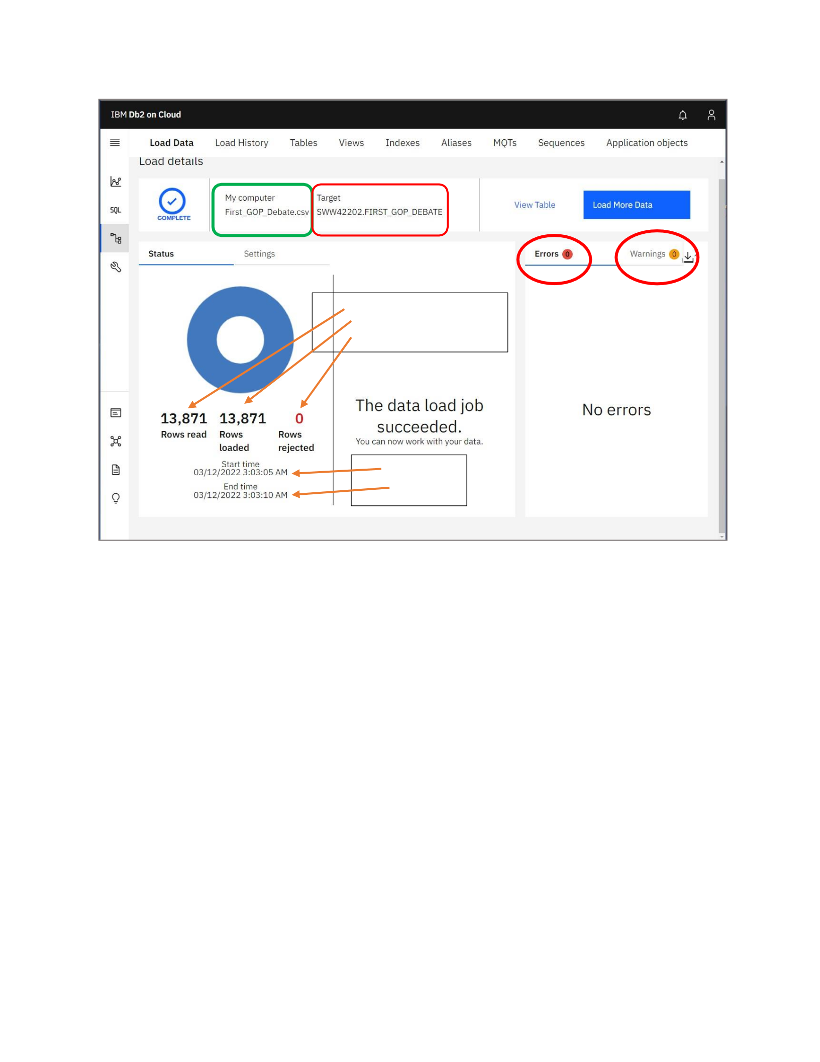
Figure 1: The Load Status Page
Dataset Validation:
In addition to the load status page, SQL and/or R can be used to validate the number of
rows in the table. Also, the ‘systable’ can be queried to confirm that the right database
instance is running, and the table structure can be seen by querying the ‘syscolumns’.
Figure 2 shows the select statement and the result that confirms the total number of rows in
the table. 13,871 rows were returned, which is the with the number of rows loaded.
• The number of Rows read
• The number of Rows loaded
• The number of Rows rejected
• Start Time
• End Time
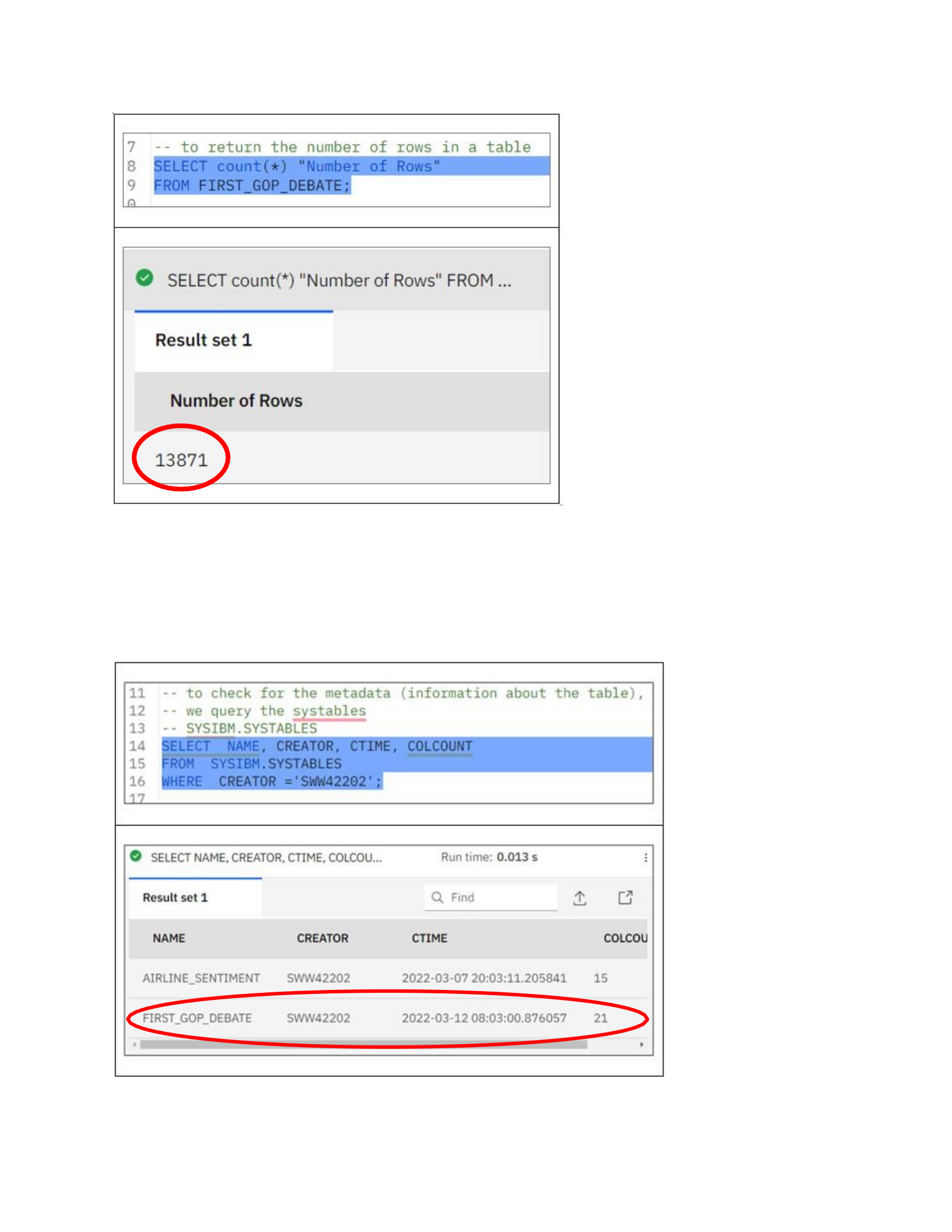
Figure 2: The Query and the Result Showing the Total Number of Rows
The information about the table was seen after the system table, ‘systable’, was quarried. The
information in the figure 3 below contains the table created and the admin username. The
table name is the ‘FIRST_GOP_DEBATE’, the administrative username is ‘SWW42202’, the
time the table was created, and the number of columns in the table were returned.
Figure 3: The Query and the Result Showing the Metadata
Dataset Manipulation - SQL:
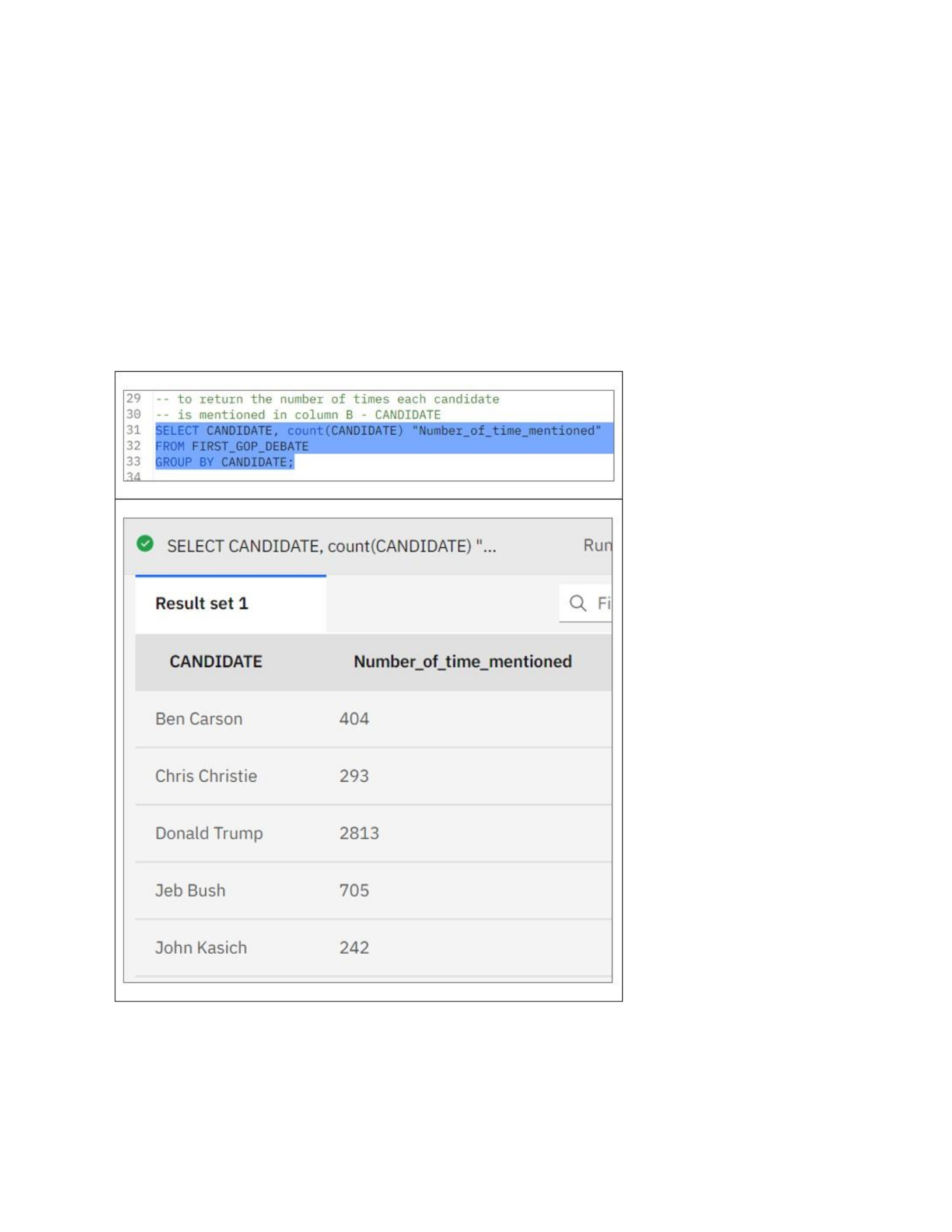
The following query will return the number of times each candidate is mentioned. To derive
this information, the ‘CANDIDATE’ column will be selected, counted, and grouped by
candidate.
The figure 4 below shows the number of times each candidate is mentioned. The output
reveals that Donald Trump is the most mentioned candidate, with total of 2,813 times, while
John Kasich was mentioned the least, with 242 times. With the margin between Donald and
the rest of the candidates, it is obvious that Donald Trump was super popular as at the time of
the first GOP debate. Being popular is of great importance and advantage to anyone running
for any position, in an election.
Figure 4: The Number of times Each Candidate is Mentioned.
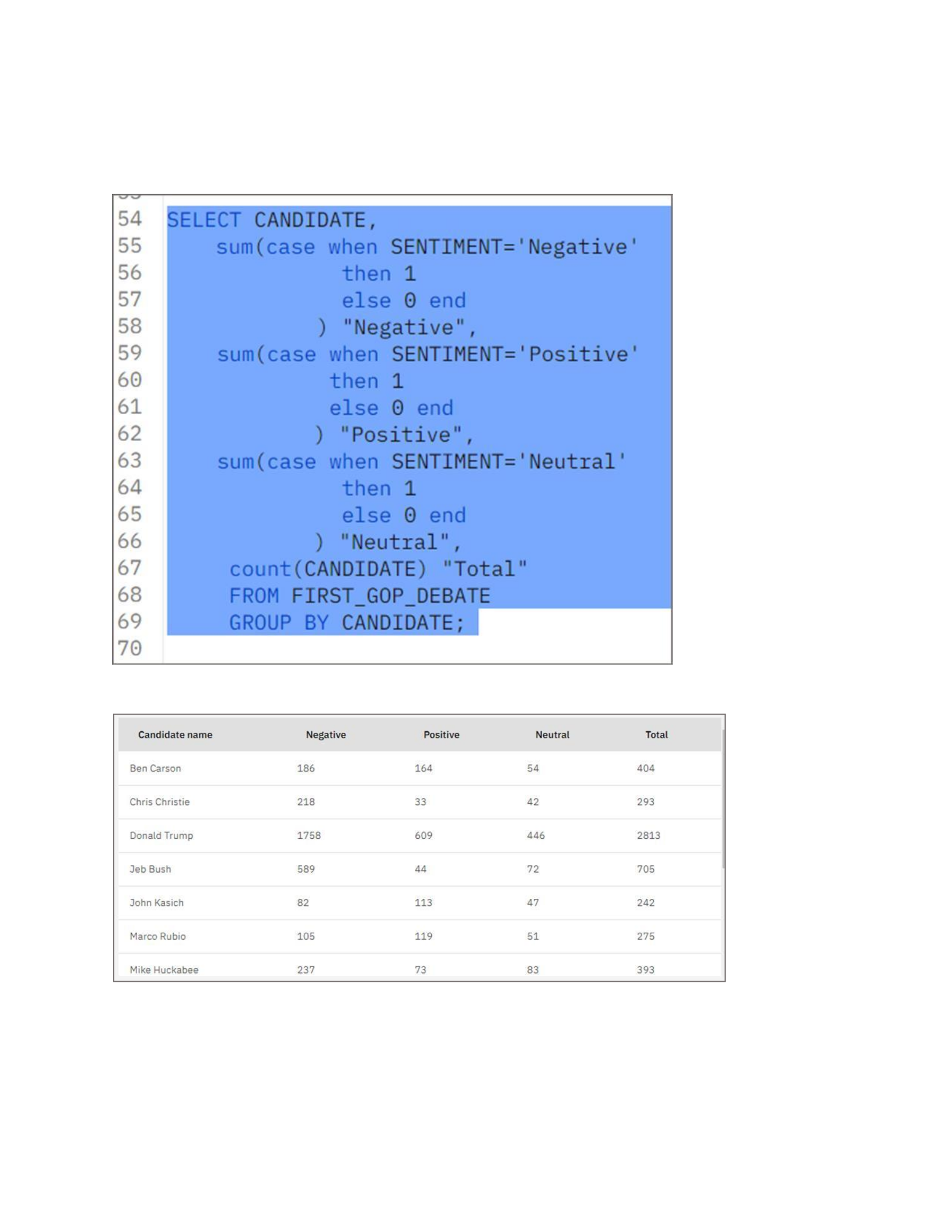
In these Twitter feeds analysis, the public sentiment is of great importance. So, the next
query will return a five-column output, to show these sentiments according to the candidates.
Figure 5a and 5b show the select statement and the result, respectively.
Figure 5a: The SQL Query to Show the Sentiments Per Candidate
Figure 5b: The Result of SQL Query to Show the Sentiments Per Candidate
Dataset Manipulation - R:
Similarly in R, the programmatic approaches used can still be verified. Having loaded the
data, R commands can be used to generate the total number of rows, view the data frame
structure, and
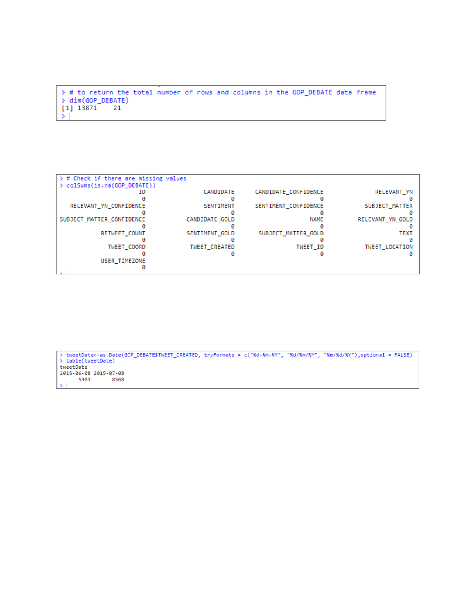
check for any missing value. The result of figure 6 below confirms that the dimension of
the table. The total number of the rows are 13,871, and the number of columns are 21.
Figure 6: The R Command Showing the Dimension of the Table.
To check if there is any missing value, the colSums command was ran, and the output shows
that there were no missing values in the table. See figure 7 below.
Figure 7: The colSums Command
It will be interesting to note that these 13,871 numbers of twit feeds were just created in 2
days. Data frame was created on the ‘TWEET_CREATED’ and the frequency of the dates
shows that the whole tweets were created in just 2 days. The figure 8 below shows the
frequency of dates.
Figure 8: The Frequency of the TWEET_CREATED – Dates
Pie Chart:
As earlier seen that Donald Trump was the most popular candidate, the pie chart below will
immediately show the margin at which he is higher than other candidates. Also, more than
half the number of the tweets do not have any candidate name.
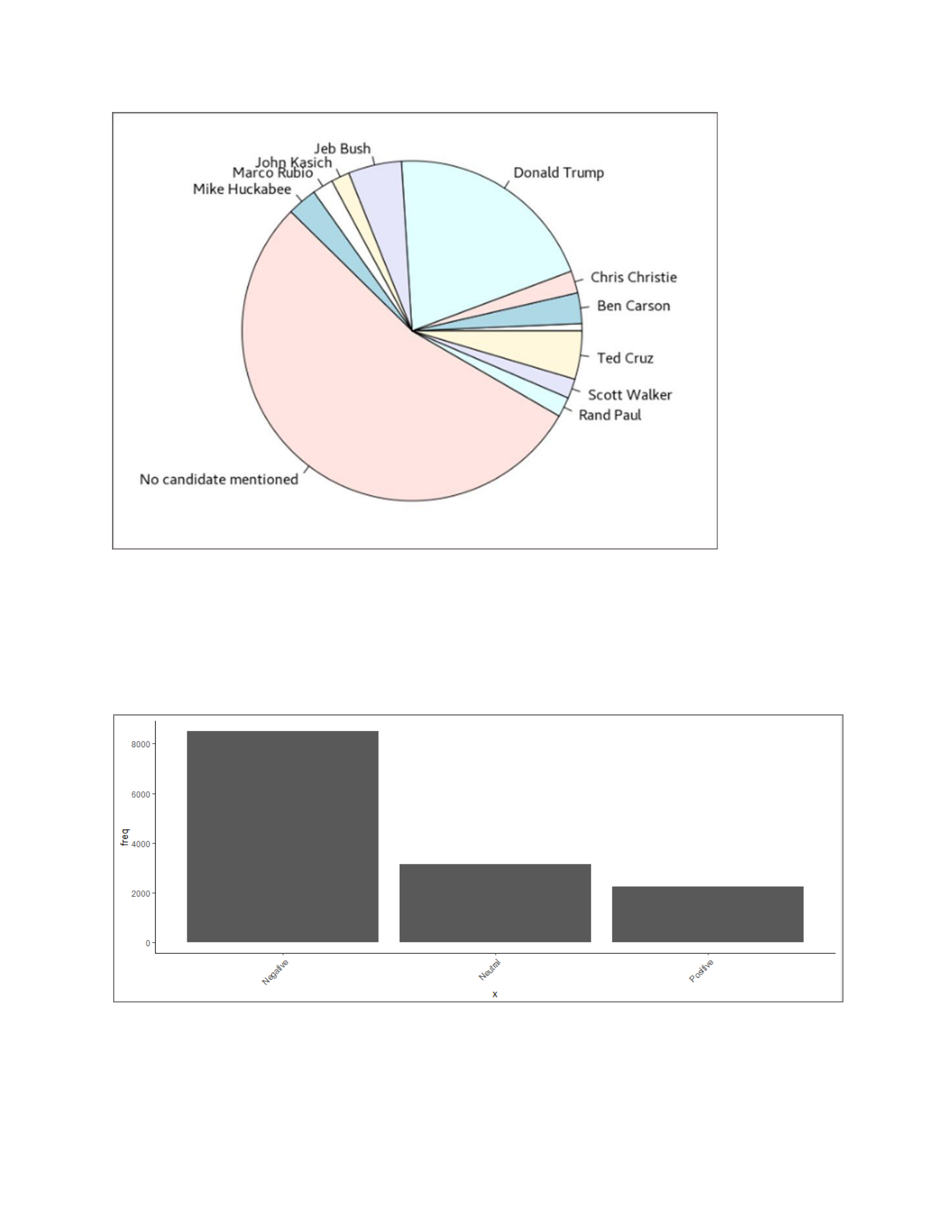
Figure 9: The Pie Chart Showing the Number of Times Each Candidate is Mentioned
Bar Chart:
The first bar chart here shows the sentiments in the tweet feeds. The Negative sentiment
stood out among the three – Positive, Negative, and Neutral. More than half of the tweet
has negative sentiment while, positive sentiment were the least.
Figure 10: The Bar Chart Showing the Tweet Sentiment
The next chart gives additional information about the candidates. Here the sentiments were
taken into consideration. The popularity of the candidate Trump is still obvious here. One
thing is
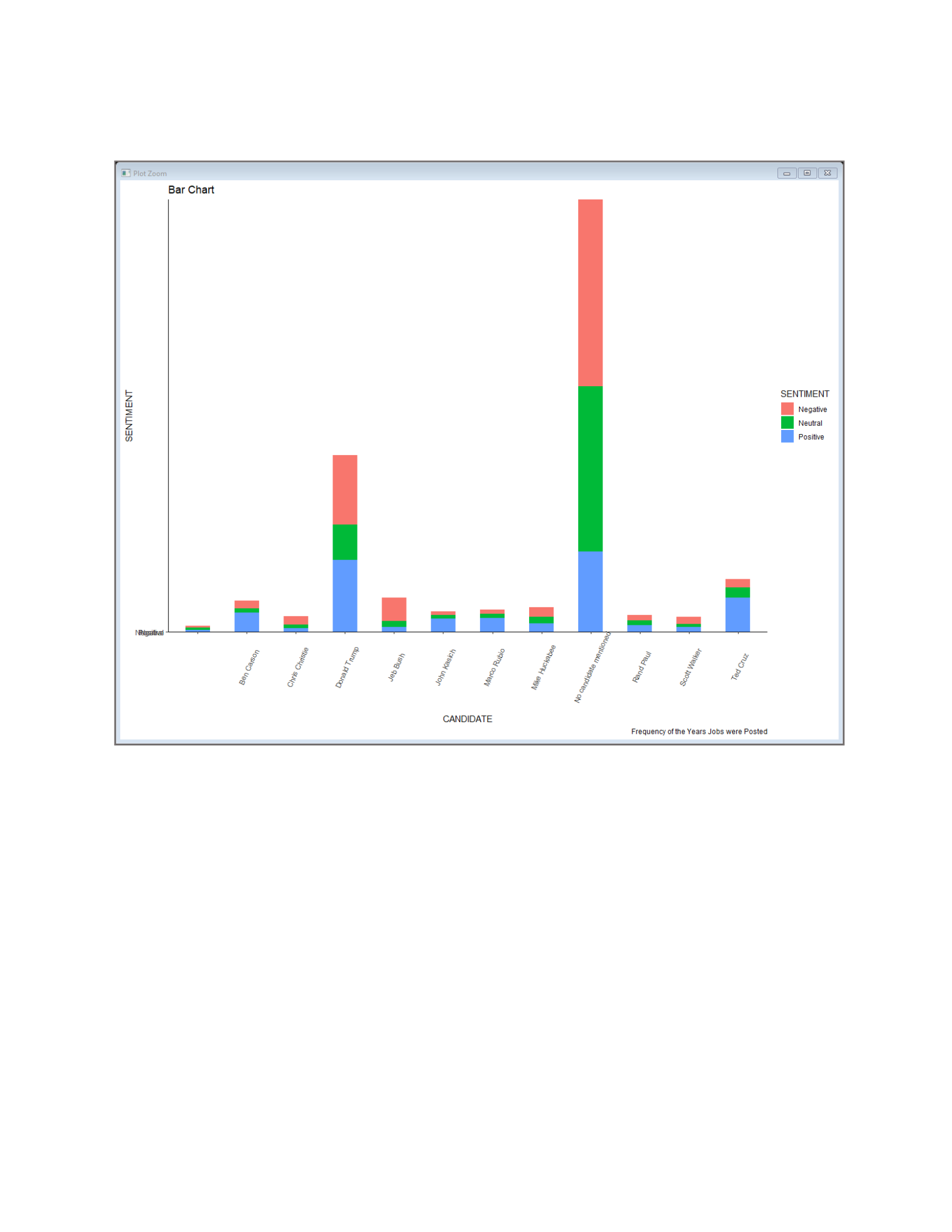
significant while, the negative sentiment tops the chart in the overall sentiment, Donald
Trump receives more of the positive sentiment than any other candidate.
Figure 11: The Sentiments Per Candidate.
Apriori:
The Apriori method is used for the Association Rule. A subset of the First GOP Debate data
frame was defined with 'CANDIDATE', 'SENTIMENT', 'SUBJECT_MATTER',
'RETWEET_COUNT', and 'USER_TIMEZONE' columns. Having done all that, the columns’
data type were changed to factor, before generating the rule, using apriori algorithm, to show
the confidence limit of 0.8 (i.e., 80%) and 0.1 (i.e., 10%) of support. In all, 1387 is the
absolute minimum support count which is 10% of the entries. Two (2) rules were generated.
Figure 12a shows the output of the Apriori rule. And figure 12b shows the gragh.
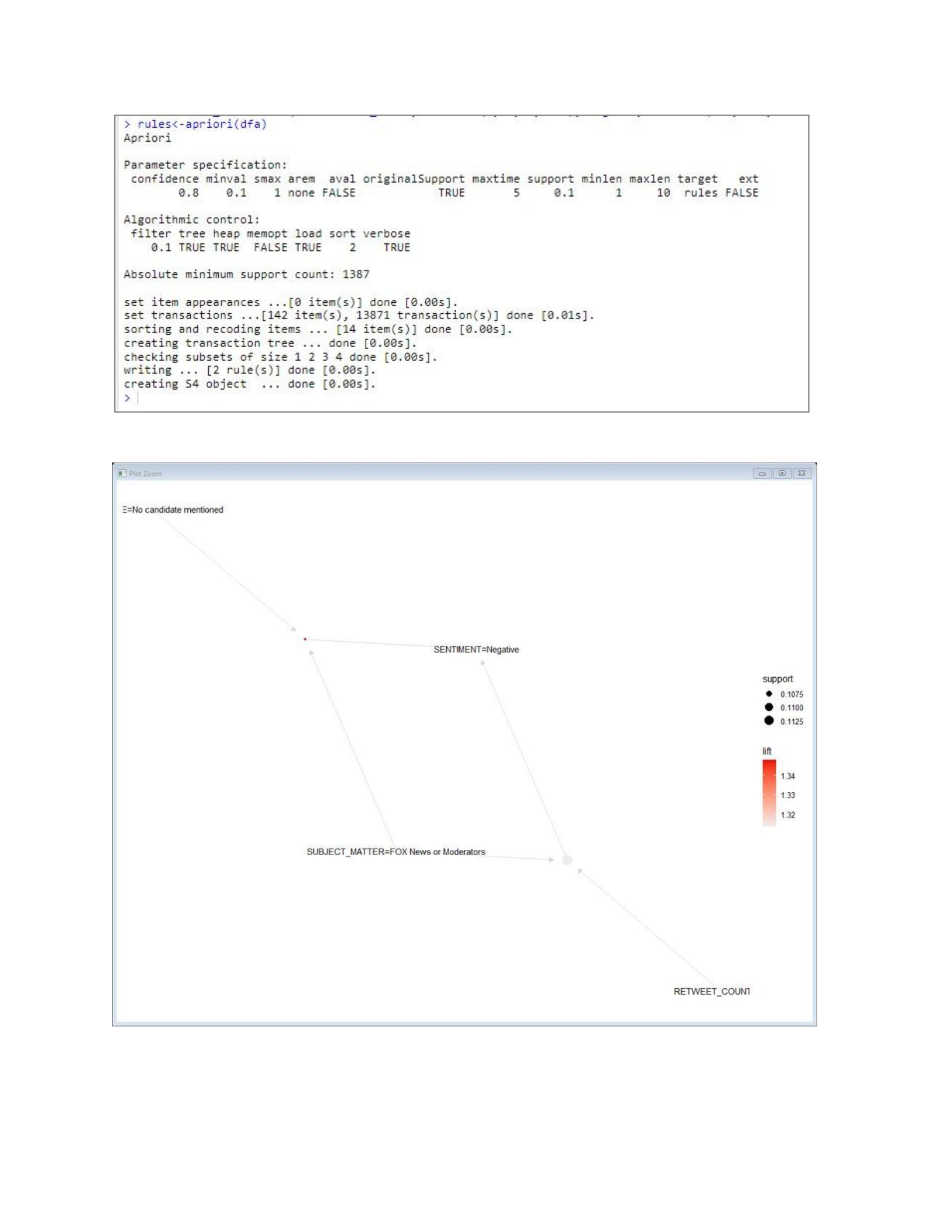
Figure 12a: The Apriori Rule
Figure 12b: The Apriori Rule Plot
WordCloud – Using the TWEET_LOCATIONS
In other to generate a WordCloud, a subset of the targeted column should be defined. Then
the single column will be converted to a vector source, after which a corpus document will
be created. This document must be free from all noise. Punctuations and stopwords must
be removed, upper letters cases must be set to lower, and the document must be stripped
from all white spaces. Only after then, that the matrix will be created and set up the
frequency count.
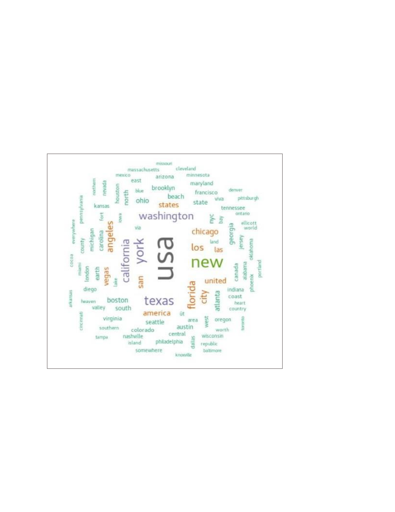
Washington, New York, Texas, and California were seen to the frequent locations where
tweets are originating from. See figure 13. These are the key cities in the United States of
America.
Figure 13: The WordCloud per Tweet Location
K-Means Cluster – Using the Positive Sentiment Tweet Text:
Like WordCloud, K-means follows the same process to produce the corpus document. After
the document were created, then k-means will be fitted and the total squared distance
between clusters and within clusters by k value will be plotted. Figure 14a and 14b the
cluster and the squared distance, respectively.
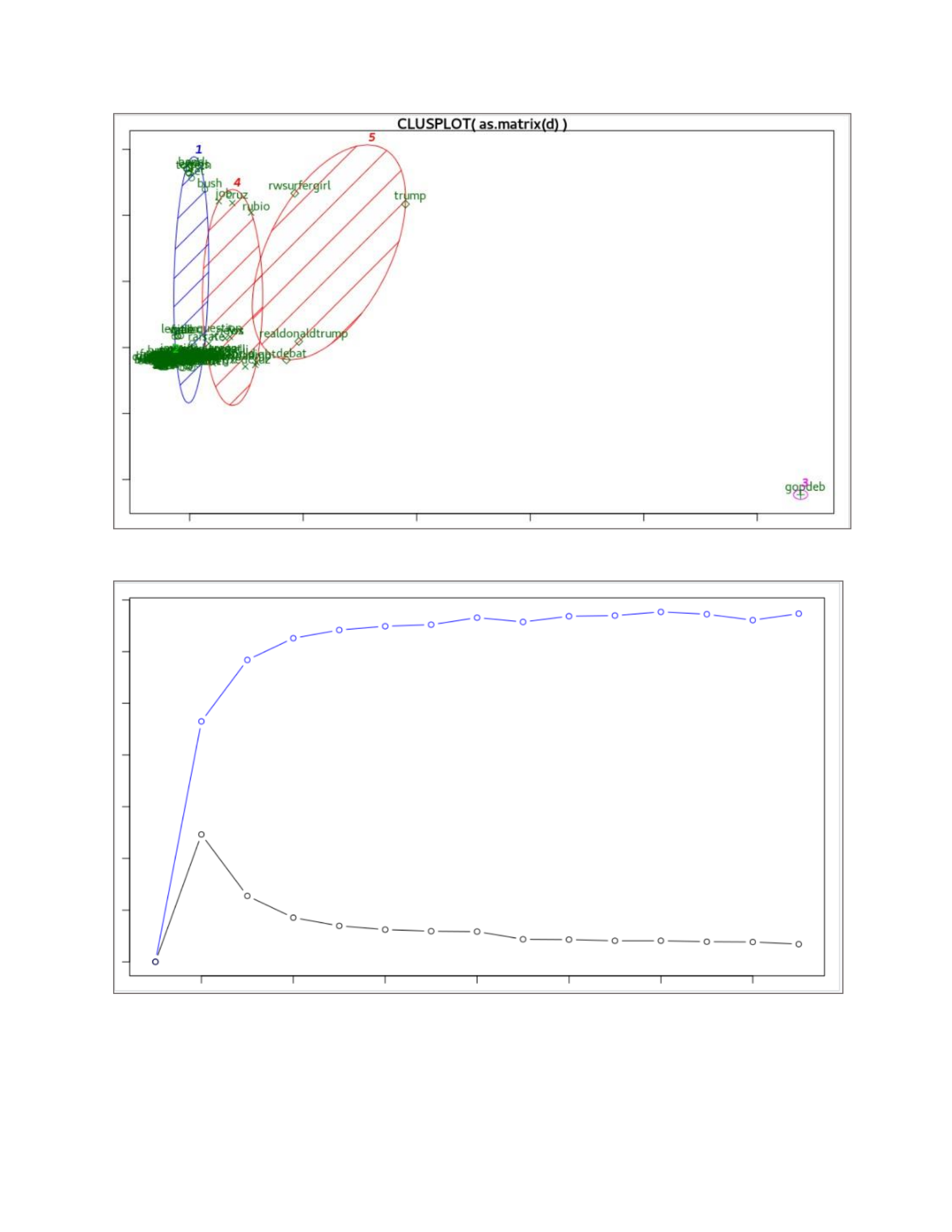
Figure 14a: The Cluster diagram
Figure 14b: The Squared Distance Between Clusters and Within Clusters

Accomplishments and Limitations:
In the process of this assignment, I was able to use this fast-growing technique –
sentiment analysis to analyze the First_GOP_Debate dataset. The insight from the
analysis shows that against all odds, negative sentiments, Donald Trump is the man of
the people. I know that I improve on the use of Cloud resources.
Beside the personal limitation I faced during the period of this assignment, I figured out
that basic knowledge of SQL and R is not enough in this type of analysis.

